Instant GaussianImage: A Generalizable and Self-Adaptive Image Representation via 2D Gaussian Splatting
Abstract
Implicit Neural Representation (INR) has demonstrated remarkable advances in the field of image representation but demands substantial GPU resources. GaussianImage recently pioneered the use of Gaussian Splatting to mitigate this cost, however, the slow training process limits its practicality, and the fixed number of Gaussians per image limits its adaptability to varying information entropy. To address these issues, we propose in this paper a generalizable and self-adaptive image representation framework based on 2D Gaussian Splatting. Our method employs a network to quickly generate a coarse Gaussian representation, followed by minimal fine-tuning steps, achieving comparable rendering quality of GaussianImage while significantly reducing training time. Moreover, our approach dynamically adjusts the number of Gaussian points based on image complexity to further enhance flexibility and efficiency in practice. Experiments on DIV2K and Kodak datasets show that our method matches or exceeds GaussianImage’s rendering performance with far fewer iterations and shorter training times. Specifically, our method reduces the training time by up to one order of magnitude while achieving superior rendering performance with the same number of Gaussians. Code is availiable at https://github.com/whoiszzj/Instant-GI
1 Introduction
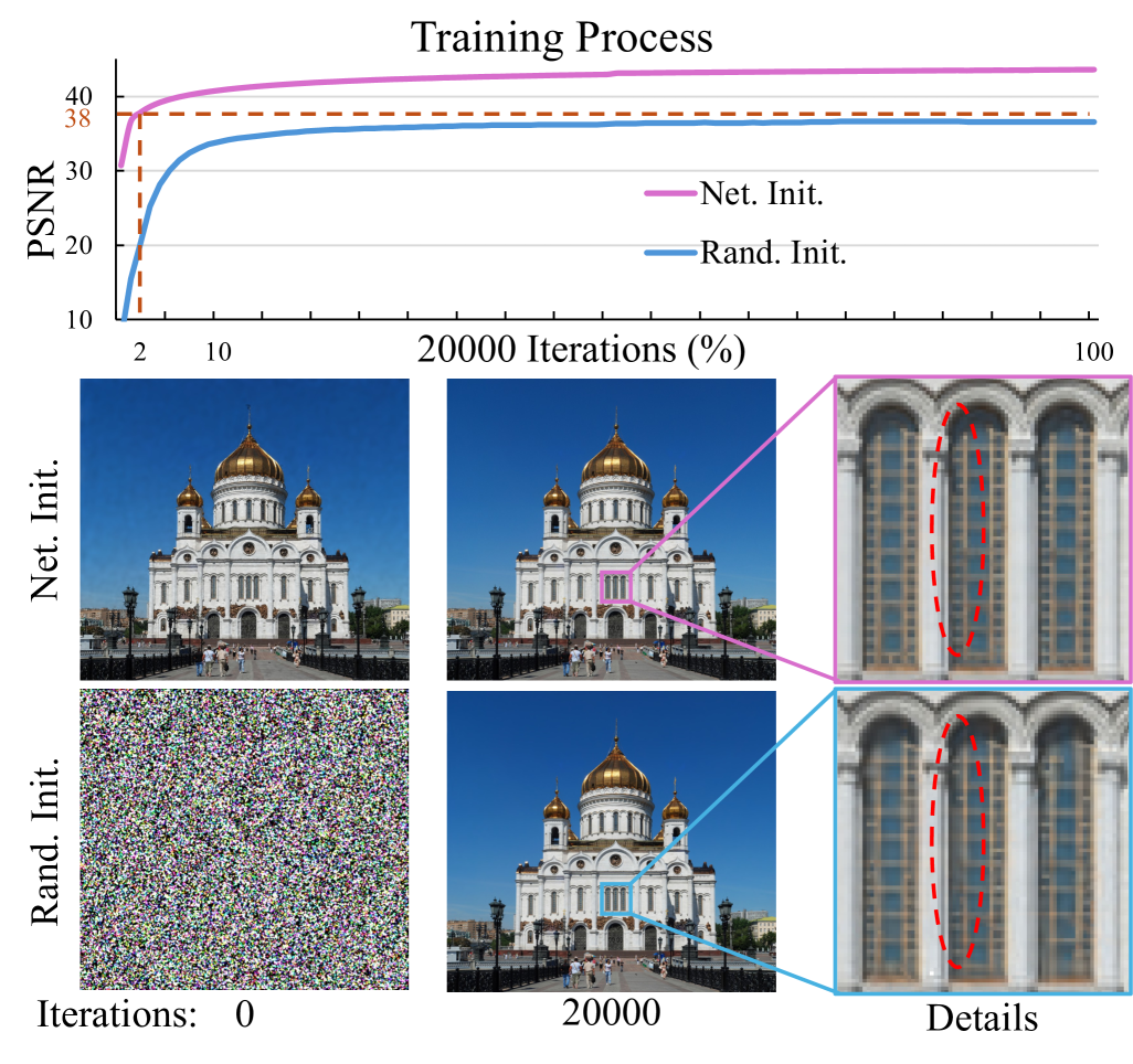
Image representation is an important task in computer vision, which has numerous applications in the fields such as image compression [38, 48], super-resolution [25, 45], deblurring [23, 34], and so on. The emergence of Implicit Neural Representation (INR) has shifted image representation from traditional methods like grid graphics to the more recent approach using multilayer perceptrons (MLPs). This method leverages the local continuity of the data to map the input coordinates to their corresponding output values.
Before the introduction of methods like GaussianImage (GI) [48], INR techniques relied primarily on high-dimensional MLPs to capture fine image details. However, this strategy leads to slower training, higher memory consumption, and longer decoding times, making it less suitable for real-world applications. To address these limitations, GI draws inspiration from 3D Gaussian Splatting [19] (3DGS), utilizing discrete Gaussian primitives for image information extraction and fitting. In addition, it employs an accumulated blending-based rasterization approach to enable fast rendering, facilitating rapid decoding. For the convenience of subsequent descriptions, we define “Gaussian Decomposition” as the process of obtaining a Gaussian representation from an image through certain operations to represent its content.
Although GI achieves decoding speeds exceeding 1000 FPS, it still faces several challenges. Firstly, the Gaussian primitives are initialized randomly, requiring a relatively long training time to achieve a stable fitting result. Secondly, the number of Gaussian primitives must be predetermined before training, which poses challenges for images with varying levels of information entropy. High-entropy images, which contain rich details and sharp transitions, require a larger number of Gaussians to capture fine details. Conversely, low-entropy images, characterized by smooth variations and fewer details, do not require as many Gaussians. Using too few Gaussians for high-entropy images may lead to loss of detail, while an excessive number for low-entropy images results in unnecessary storage overhead and reduced rendering efficiency.
To resolve these issues and improve the rendering performance of GI, we propose to utilize a generalizable network to initialize Gaussian representation, enabling a more efficient Gaussian Decomposition through a single feedforward pass. To this end, we propose a novel pipeline for Gaussian Decomposition, named as Instant GaussianImage (Instant-GI). Specifically, given an input image, we first employ a feature extraction network to generate a feature map, from which a Gaussian Position Probability Map (PPM) is derived. The PPM is then discretized using the Floyd–Steinberg dithering [14] algorithm, allowing for a flexible number of Gaussians to adapt to images with varying levels of information entropy. Finally, based on the dithering result and feature map, the full set of Gaussian attributes are predicted, and the entire network is trained via a differentiable rasterization for self-supervised learning.
With the proposed generalizable network, a high-quality Gaussian representation can be quickly initialized for an image. Followed by minimal fine-tuning steps, it can match or exceed the results obtained by GI through long training, as shown in Fig. 1. Furthermore, our method adaptively determines the number of Gaussians based on the information entropy of the image, ensuring both efficiency and flexibility between different images. Our main contributions are summarized as follows.
-
•
We propose a generalizable network for fast Gaussian Decomposition, enabling efficient initialization that significantly reduces training time.
-
•
We introduce the Floyd–Steinberg dithering algorithm to discretize the Gaussian PPM, allowing for adaptive and optimal spatial distribution of point cloud based on an image’s information entropy.
-
•
We develop a novel pipeline for Gaussian Decomposition that generates a high-quality Gaussian representation in a single feedforward pass.
-
•
Numerical experiments on DIV2K and Kodak datasets demonstrate that our method, with much shorter training times, achieves results comparable or superior to GI.
2 Related Work
2.1 Implicit Neural Representation
Implicit Neural Representation hass been widely applied in various domains due to their ability to represent continuous spatial information, including 3D scene representation [33, 2, 43, 3], image and video representation [35, 36, 9, 8, 7], compression [24, 41, 38], and super-resolution [12, 27, 16, 25]. In image representation, [21] introduces a hypernetwork-based functional representation, mapping coordinates to colors for continuous reconstruction. To mitigate spectral bias, [39] proposes Fourier feature mapping, while [37] leverages periodic activation functions for improved detail modeling. [9] bridges discrete and continuous representations by predicting RGB values from coordinates and local deep features. Recent works have explored adaptive and efficient INR designs. [32] proposes a hybrid implicit-explicit model with multiscale decomposition for gigapixel images. [35] employs multiresolution hash encoding to accelerate training and rendering. [11] introduces neural fields with adaptive radial bases, improving detail capture. Additionally, [4] encodes discontinuities using Bézier curves and triangular meshes to enhance sharp feature preservation and compression efficiency.
2.2 Gaussian Splatting
3DGS [19] has gained significant attention in 3D scene reconstruction due to its fast training, efficient rendering, and high-quality results. Its differentiable rasterization process has also been applied to various domains, including depth map rendering for geometric reconstruction [17, 46, 6, 47], 3D model generation via diffusion [50, 26, 40], and 3D scene editing [10, 18, 44]. Several works have extended 3DGS to enhance its effectiveness. Scaffold-GS [31] integrates anchor points and scene features to improve Gaussian property prediction. MVSGaussian [28] leverages MVSNet for image-based feature extraction, followed by 3D convolution to estimate spatial point positions and predict Gaussian attributes. DiffGS [50] introduces a disentangled representation of 3D Gaussians, enabling flexible and high-fidelity Gaussian generation for rendering.
2.3 GS-based Image Representation
In recent years, several methods have integrated Gaussian Splatting with image representation. One of the most notable is GaussianImage [48], which replaces traditional sorting-based splatting with an accumulated blending-based rasterization method. This enables faster training and rendering while achieving high-ratio image compression. Image-GS [49] adopts a similar approach, computing grayscale gradients to generate probability values, which are then used for CDF-based Gaussian sampling and initialization. GaussianSR [15] uses Gaussian Splatting’s interpolation capabilities for super-resolution by converting an image into a feature map, generating a high-resolution feature representation and reconstructing the final output with a decoder. Mirage [42] extends GI by projecting 2D images into 3D space, employing flat-controlled Gaussians for precise 2D image editing.
In this paper, we adopt GI as the baseline of our proposed work. Since our Gaussian model remains consistent with GI, all compression techniques for GI from [48] can be applied directly to our method. Therefore, we do not elaborate on this aspect. Instead, our primary goal focuses on fast and effective initialization to significantly enhance training speed and rendering performance.
3 Proposed Method
3.1 Preliminaries
GI refines the Gaussian model based on 3DGS to enhance image representation performance, and our proposed method is also built upon this foundation. Note that a 2D Gaussian is characterized by the following attributes: position , 2D covariance matrix , color parameter , and opacity .
For the positive semidefinite covariance matrix, GI offers two different parameterization approaches. The first approach employs Cholesky factorization, directly decomposing the covariance matrix into a lower triangular matrix , such that . The second approach, similar to 3DGS, decomposes into a scaling matrix and a rotation matrix :
| (1) |
where
| (2) |
For ease of transformation, our method primarily adopts the parameterization for learning and representation.
The learnable Gaussian parameters are optimized through differentiable rasterization. Unlike 3DGS, which needs to handle occlusion, GI does not require opacity accumulation or Gaussian sorting. Consequently, the rendering equation is given by:
| (3) |
where represents the set of Gaussians contributing to the rendering of the pixel, and
| (4) |
where denotes the displacement between the pixel center and the projected 2D Gaussian center. Since both opacity and color are learnable parameters, GI integrates them together, which can be expressed as:
| (5) |
In this case, the parameters of the Gaussian model consist of the position, covariance matrix, and color attributes – a total of eight learnable parameters. During initialization, the number of Gaussians is determined and remains fixed throughout training. The position parameters are uniformly sampled from . The scaling parameters are initialized randomly in , while the rotation angle is drawn from . Similarly, the color attributes are randomly initialized within . Such purely random initialization lacks prior guidance, making the optimization process slower in deriving an accurate Gaussian representation of the image.
3.2 Overview
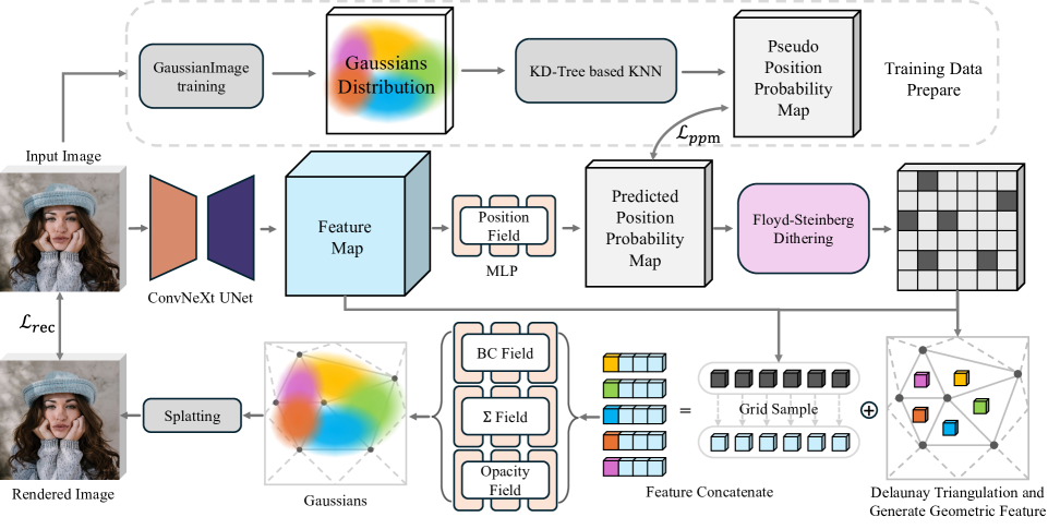
Our Instant-GI framework is illustrated in Fig. 2. In the following sections, we introduce the main modules of our framework. Given an image of size , our objective is to obtain its Gaussian representation using Instant-GI. We begin by employing a ConvNeXt-based [29] UNet to extract features from the image. Based on these extracted features, a self-adaptive number of Gaussians are generated. Then, the corresponding parameters are produced for each Gaussian to ensure that the splatting process generates a rendering result consistent with the input image. To achieve this goal, our work broadly consists of three parts: (1) how a self-adaptive number of Gaussians is generated from the extracted features, (2) how the features of each Gaussian are structured and transformed into appropriate Gaussian parameters, and (3) which loss functions are used to ensure that the entire network is trained effectively.
3.3 Self-Adaptive Gaussian Samples
To enable the algorithm to adaptively determine the number of Gaussians for images with varying levels of information entropy, ensuring consistent rendering performance across different images, intuitively:
-
•
The higher the information entropy of an image, the greater the number of Gaussians required.
-
•
Within different regions of an image, areas with higher entropy should have a higher density of Gaussian.
A natural approach is to compute the color gradient of the image and use it to determine the Gaussian density, ensuring that regions with higher color gradients contain more Gaussians to capture high-frequency information. For instance, [49] computes the probability of generating a Gaussian based on the gradient of the pixel and sampled with Cumulative Distribution Function (CDF). However, the distribution of an image’s Gaussian representation does not strictly correspond to variations in the color gradient. While the color gradient may exhibit abrupt changes, the variation in Gaussian density tends to be smoother (demonstrated in Fig. 5 in Sec. 4). As a result, directly deriving the probability of Gaussian generation from the gradient is suboptimal. To address this, we adopt a data-driven approach by training a network to predict the probability of Gaussian generation more effectively.
Obtain Pseudo PPM. To train a network capable of predicting a Position Probability Map (PPM) that indicates the spatial distribution of Gaussians, we first generate high-quality training data by Gaussian Decomposition. After that, we compute the Gaussian density at each pixel position in the image. Specifically, for each , we estimate the minimal radius of a circle centered on that encompasses Gaussians, then the local Gaussian density is defined as the unit density of Gaussians in this circle:
| (6) |
where represents the position coordinates, and indexes the top- nearest neighbors of . In our experiments, we set . Next, we convert this density map into a PPM, which determines the probability of generating a Gaussian at each pixel location:
| (7) |
Finally, under the supervision of , we use an MLP network (Position Field in Fig. 2) to predict . For more details of the generation of , please refer to the supplementary material.
Dither with . The key challenge is how to sample Gaussians based on the PPM. A straightforward approach is thresholding—sampling a Gaussian if its probability exceeds a certain value. However, this ignores spatial dependencies, leading to excessive Gaussians in high-entropy regions and sparse coverage in low-entropy regions, resulting in underfitting and overfitting [19]. An alternative is CDF sampling with a fixed number of Gaussians, as in [49]. While it works when high- and low-entropy regions are balanced, it degrades rendering quality when high-entropy regions dominate, reducing point density where detail is needed. Conversely, in low-entropy images, excessive points are allocated to smooth regions, leading to redundancy (refer to supplementary material for details).
To address this, before generating the Gaussian, we adopt the Floyd–Steinberg Dithering algorithm [14] to adaptively discretize the PPM. The map is firstly divided into patches, with each patch assigned its highest probability as the representative value. We then apply dithering and use the centers of the activated patches as sampling points, ensuring a balanced spatial distribution.
3.4 Transformation from Feature to Gaussians
Ellipse Fitting. From the previous steps, we obtain a set of discrete points whose distribution reflects the image’s entropy information. However, to fully define the Gaussians, we still need to predict their scaling, rotation, and color.
Since the scaling is measured in pixel units, directly predicting an absolute value with the network is hard work. Instead, a reference value is required to constrain the learning range, similar to [31]. To better determine the learning range for scaling, we introduce the Delaunay Triangulation [5] method for help based on two insights:
-
•
Given that the scaling defines a Gaussian as an ellipse, the overlap between ellipses should be minimized to reduce the network’s learning complexity.
-
•
Simultaneously, all ellipses should fully cover the entire image to prevent underfitting.
Specifically, we perform Delaunay Triangulation on the discrete points, using the resulting triangles as fundamental feature processing primitives as they can guarantee full coverage without overlap. For the obtained set of triangle representations , where each consists of the three vertex coordinates of the corresponding triangle:
| (8) |
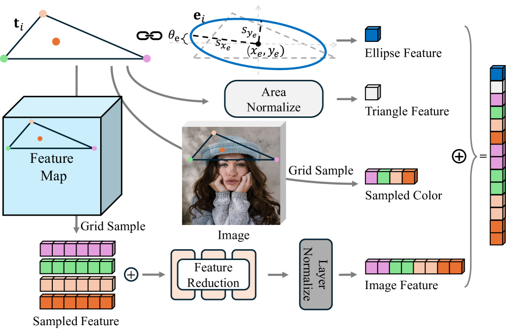
Next, we compute the midpoints of the three edges of each triangle to extract additional geometric information. Using these six points, we perform ellipse fitting [13] to obtain the set of ellipses , where each ellipse is characterized by its position, major and minor axes, and rotation parameters:
| (9) |
For more details, please refer to the supplementary material.
Feature Organization After obtaining the fitted ellipse for each triangle, the next step is to extract the corresponding feature information for each primitive. As illustrated in Fig. 3, given the triangle and its fitted ellipse , we compute the triangle and ellipse features, which serve as geometric attribute inputs to the network. Additionally, we sample both the image and the feature map at the three triangle vertices and the center point to obtain the corresponding color and feature values. To prevent an excessively high feature dimension, we apply feature reduction and layer normalization to the sampled features. The four feature components are concatenated to form the final feature vector, which is fed into the Gaussian fields. For more details, please refer to the supplementary material.
Gaussian Fields. After extracting the features of each primitive, we predict all Gaussian attributes based on these features, including position, scaling, rotation, and color.
When predicting position information, we use the “BC Field” in Fig. 2 to compute the barycentric coordinates of the Gaussian center . The final Gaussian position is obtained as:
| (10) |
When predicting the scaling and rotation parameters, we use a single MLP, denoted as the “ Field” in Fig. 2. Given the major and minor axes and the rotation angle of a fitted ellipse, our predictions include the scaling adjustment factors and the rotation bias . The activation function applied to is defined as:
| (11) |
The final scaling is computed as:
| (12) |
The final rotation is obtained as:
| (13) |
where is the sigmoid function, and is the inverse.
When predicting color attributes, we found that directly regressing RGB values from features results in slow convergence during early training stages and may even lead to training failure. Thus, we predict the opacity attribute with the “Opacity Field” in Fig. 2 instead of directly predicting color. The final color attribute is then obtained by multiplying the color sampled from the image at the Gaussian position with the opacity:
| (14) |
At this point, all the attributes of each Gaussian primitive have been initialized as:
| (15) |
3.5 Loss Function
To ensure network training, the initialized Gaussian primitives are rendered into an image using the splatting technique. The primary objective of the network is image reconstruction, optimized via the loss function , which combines the loss and the D-SSIM term:
| (16) |
Furthermore, to supervise the PPM, we introduce the loss function , formulated as a Focal MSE Loss:
| (17) |
The overall optimization objective is defined as:
| (18) |
4 Experiments
4.1 Experimental Setup
Dataset. Following GI, we evaluate our method on the Kodak [22] and DIV2K [1] datasets. The Kodak dataset consists of 24 images, each with a resolution of . The DIV2K dataset contains a training set of 800 images and a test set of 100 images. For network training, we utilize images from the DIV2K training set, applying bicubic downscaling at scales , , and . During evaluation, to ensure consistency with GI and other methods, we conduct testing at a scale of on the test set, with image dimensions ranging from to .
Implementation. We set patch size in Sec. 3.3 during training, while during testing, different levels such as can be used to further control the number of Gaussians. To accelerate Floyd–Steinberg dithering, we implement a GPU-accelerated version based on [14]. For loss parameter settings, we set , , and . We use the Adam [20] optimizer with a cosine annealing scheduler [30], where the learning rate decays from to over 100 epochs. For the subsequent fine-tuning stage, we follow the same experimental settings as GI. Our method is trained and tested on one NVIDIA A100 (40GB). For more details, please refer to the supplementary material.
| Datasets | Kodak | DIV2K 2 | ||||
|---|---|---|---|---|---|---|
| Methods | PSNR | MS-SSIM | Params(K) | PSNR | MS-SSIM | Params(K) |
| WIRE | 41.47 | 0.9939 | 136.74 | 35.64 | 0.9511 | 136.74 |
| SIREN | 40.83 | 0.9960 | 272.70 | 39.08 | 0.9958 | 483.60 |
| I-NGP | 43.88 | 0.9976 | 300.09 | 37.06 | 0.9950 | 525.40 |
| NeuRBF | 43.78 | 0.9964 | 337.29 | 38.60 | 0.9913 | 383.65 |
| 3DGS | 43.69 | 0.9991 | 3540.00 | 39.36 | 0.9979 | 4130.00 |
| GI | 44.08 | 0.9985 | 560.00 | 39.53 | 0.9975 | 560.00 |
| GI† | 41.44 | 0.9979 | 342.86 | 40.26 | 0.9980 | 615.05 |
| Ours | 42.92 | 0.9972 | 342.86 | 42.80 | 0.9982 | 615.05 |
| Image ID | Gaussian Num. | Init. Method | PSNR | GPU Mem. (MB) | Training FPS | Testing FPS | ||
| 2s | 10s | 20s | ||||||
| 08442 | 60170 | Rand. Init | 35.14 | 44.75 | 45.90 | 410 | 717 | 3015 |
| Net. Init. | 46.68 | 49.05 | 49.58 | 3038 + 408 | 447 | 1969 | ||
| 08792 | 77690 | Rand. Init | 31.96 | 36.04 | 36.47 | 454 | 582 | 2506 |
| Net. Init. | 37.41 | 41.51 | 42.49 | 3624 + 466 | 344 | 1536 | ||
| 08582 | 82766 | Rand. Init | 32.25 | 36.58 | 37.12 | 414 | 736 | 2733 |
| Net. Init. | 36.79 | 39.72 | 40.51 | 3038 + 414 | 718 | 2740 | ||
4.2 Quantitative Results
This experiment aims to demonstrate the upper bounder of rendering performance achievable by our method. We compare our approach with several recent image representation methods, with the specific results shown in Tab. 1. In this experiment, both our method and GI undergo extensive training (50,000 iterations).
Firstly, our method achieves state-of-the-art (SOTA) performance on the DIV2K dataset. Secondly, compared to GI†, our method outperforms in final rendering quality under the same number of Gaussians. This is due to our initialization aligning better with image information entropy, reducing optimization complexity, and enhancing rendering quality. Thirdly, while our method does not surpass GI on the Kodak dataset, this is primarily due to Kodak’s lower resolution, leading to a 61% reduction in Gaussian points. However, across both datasets, our method demonstrates a more stable performance (PSNR: 42.92 on Kodak, 42.80 on DIV2K ), proving its ability to dynamically adjust Gaussian counts based on information entropy for consistent image representation. In summary, our method enables a well-structured distribution with an optimized number of Gaussians, reducing the computational complexity of optimization while improving rendering quality.
4.3 Performance & Qualitative Results
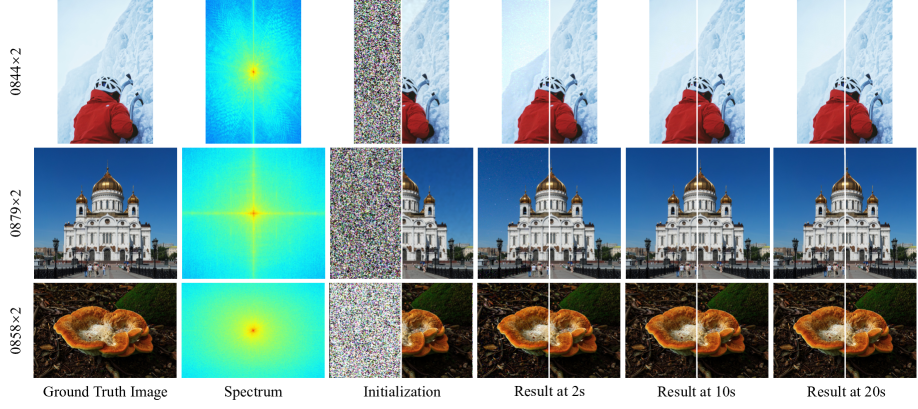
One of the key contributions of our algorithm is its ability to achieve usable rendering results within a short time. Therefore, we specifically analyze this performance in this subsection. In this experiment, we select three representative images: one with predominantly low-entropy information, one with a balance of high and low entropy, and one with predominantly high-entropy information. We compare GI with random initialization and our network-based initialization, reporting PSNR at 2s, 10s, and 20s (including initialization time) for both methods. As shown in Tab. 2, our initialization significantly accelerates rendering. For images 08442 and 08792, the 2s rendering surpasses random initialization at 20s, achieving over a 10 speed-up. Even for 08582, which predominantly contains high-entropy regions and exhibits a spatial distribution similar to random initialization, our method still achieves a 5 speed-up by predicting more accurate scaling, rotation, and color parameters. Regarding memory usage, our method requires approximately 3GB due to additional network computations, but this is negligible for modern GPUs.
In Fig. 4, we present the frequency spectrum analysis, initialization results, and rendered outputs at different time intervals for three selected images. From the initial rendering, our method already achieves high-quality results, with only minor deficiencies in fine details. By 2s, the rendering output becomes visually indistinguishable from the ground truth, whereas the random initialization method remains unconverged, exhibiting significant artifacts. At 10s and 20s, both methods produce nearly identical results. However, upon closer inspection, fine-grained differences persist, as illustrated in Fig. 1. Additional results can be found in the supplementary material.
Based on the above observations, we conclude that our algorithm achieves high-quality rendering immediately after network-based initialization. With only 2 seconds of initialization and fine-tuning, our method attains rendering quality comparable to GI after 20+ seconds of training, significantly improving the efficiency.
4.4 Ablation Study
We conduct four ablation experiments to validate the rationality of our proposed method, as summarized in Tab. 3. These experiments aim to answer the following questions:
-
•
Why can’t the PPM be directly derived from image gradient but instead needs to be learned through network?
-
•
Why not directly predict color but learn opacity?
-
•
Why don’t we initialize directly with the fitted ellipse?
-
•
If the number of points in an image is self-adaptive, how can different compression ratios be achieved?
| Method Describe | Gaussian Num. | Initialization | 2s | ||
|---|---|---|---|---|---|
| PSNR | MS-SSIM | PSNR | MS-SSIM | ||
| Dither with Img. Grad. | 51675 | 27.15 | 0.9347 | 37.42 | 0.9934 |
| Color Field | 77451 | 30.21 | 0.9740 | 38.49 | 0.9968 |
| Init. with Fitted Ellipse | 76881 | 17.87 | 0.6942 | 36.94 | 0.9968 |
| Ker. Size = 4 (w/o train) | 43627 | 24.31 | 0.8911 | 35.12 | 0.9936 |
| Ker. Size = 4 (train) | 44639 | 29.53 | 0.9724 | 35.99 | 0.9945 |
| Final | 76881 | 30.26 | 0.9752 | 38.73 | 0.9968 |
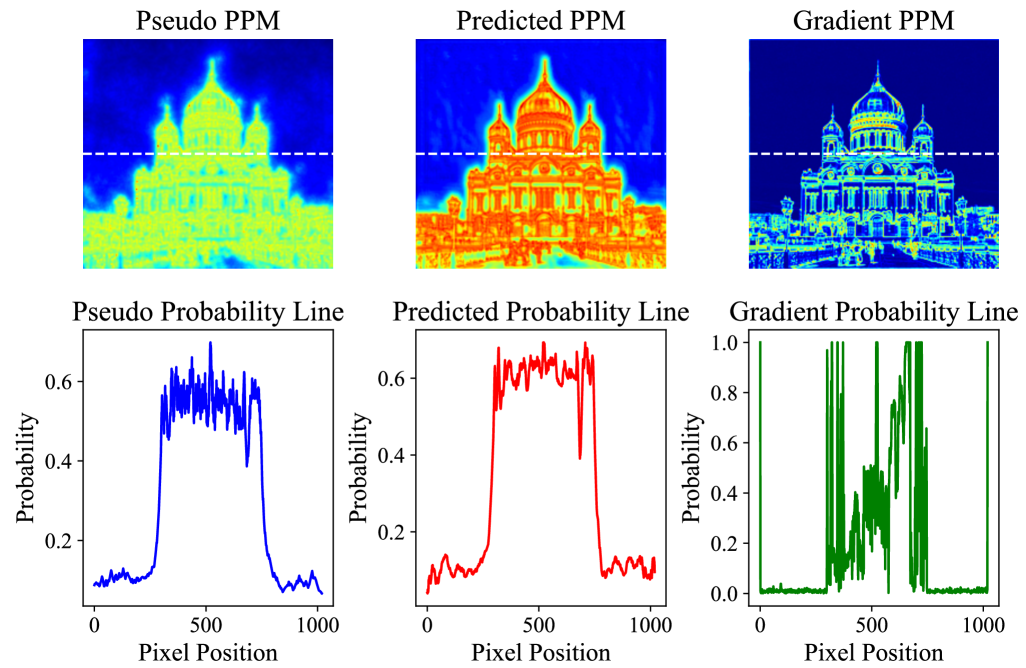
Dithering using Image Gradient. In Sec. 3.3 we point out that gradient-based sampling is sub-optimal. The key issue, as observed in our experiments, is that high-entropy regions tend to have dense point distributions, while low-entropy regions are sparsely populated. However, at the boundaries between these regions, a smooth transition is necessary. Gradient-based probability maps rely solely on local information and fail to capture the overall density distribution. As shown in Fig. 5, analyzing probability values along the horizontal center of the image reveals that both our method and the pseudo-probability distribution exhibit smooth transitions. In contrast, gradient-based maps introduce abrupt changes at high-low entropy boundaries, resulting in uneven density distributions and poor transitions. Essentially, a gradient-based probability map acts as an edge detector, leading to excessive sampling along edges while significantly reducing point density in smooth regions. This imbalance yields fewer total samples and, as Tab. 3 confirms, degrades rendering quality.
Color Field. In Sec. 3.4, we proposed learning opacity and sampling colors from the image rather than directly predicting color as GI. This reduces the number of learned parameters from three (RGB with opacity) to one (opacity). On one hand, this approach does not compromise the model’s expressive capability, as shown in Table 3. On the other hand, directly learning color slows down training and increases the likelihood of getting stuck in local minima. Please refer to the supplementary material for more details.
Initialization with Fitted Ellipse. As mentioned in Sec. 3.4, the fitted ellipse acts a reference for each primitive. So, why not use it directly for Gaussian initialization? As shown in Tab. 3, initializing Gaussians directly with the fitted ellipses can’t yield reasonable scaling, rotation, and color. Additionally, at 2s, the PSNR of this method is lower than that obtained through network-based initialization.
Kernel Size = 4. A key feature of our algorithm is its ability to automatically determine the optimal number of Gaussians for a given image. But how can we achieve different compression ratios? As discussed in Sec. 3.3, our method controls the number of generated points by setting a kernel size . Increasing will reduce the number of generated points. Our model was trained with , achieving a well-optimized image representation. However, we can directly apply to the same model without retraining. The corresponding rendering results are shown in Tab. 3 as “Kernel size = 4 (w/o train)”. Similarly, we can fine-tune the model trained with to adapt to , with the corresponding rendering performance listed as “Kernel size = 4 (train)” in Tab. 3. From the results, we observe that our method still produces a good result even without retraining, and fine-tuning significantly improves initialization quality. Meanwhile, the number of generated points decreases, effectively achieving a higher compression ratio.
5 Conclusion
In this paper, we propose Instant-GI, a generalizable and self-adaptive image representation framework based on 2D Gaussian Splatting. Our method generates high-quality Gaussian representations through a single feedforward pass, followed by minimal fine-tuning to match or surpass the rendering performance of GI, which requires significantly longer training. Furthermore, our approach adaptively determines the number of Gaussians based on the image information entropy, ensuring consistent performance across different datasets. Experimental results in the DIV2K and Kodak datasets show that, given the same number of Gaussians, Instant-GI achieves a rendering performance comparable to or surpass GI while significantly reducing training times. These findings underscore efficiency and practicality of our approach for high-quality image representation. For future work, we aim to further enhance rendering quality by exploring alternative initialization and optimization strategies. Our current pipeline incurs notable CPU overhead, particularly in Delaunay Triangulation, which could be optimized for better efficiency. Lastly, scaling our method to larger datasets may further improve its performance, contributing to a more robust image representation framework.
6 Acknowledgements
This work is supported by the Natural Science Foundation of China under Grant 62302174. The computation is completed in the HPC Platform of Huazhong University of Science and Technology. We also thank Farsee2 Technology Ltd for providing devices to support the validation of our method.
References
- Agustsson and Timofte [2017] Eirikur Agustsson and Radu Timofte. Ntire 2017 challenge on single image super-resolution: Dataset and study. In Proceedings of the IEEE conference on computer vision and pattern recognition workshops, pages 126–135, 2017.
- Barron et al. [2021] Jonathan T Barron, Ben Mildenhall, Matthew Tancik, Peter Hedman, Ricardo Martin-Brualla, and Pratul P Srinivasan. Mip-nerf: A multiscale representation for anti-aliasing neural radiance fields. In Proceedings of the IEEE/CVF International Conference on Computer Vision, pages 5855–5864, 2021.
- Barron et al. [2023] Jonathan T. Barron, Ben Mildenhall, Dor Verbin, Pratul P. Srinivasan, and Peter Hedman. Zip-nerf: Anti-aliased grid-based neural radiance fields. ICCV, 2023.
- Belhe et al. [2023] Yash Belhe, Michaël Gharbi, Matthew Fisher, Iliyan Georgiev, Ravi Ramamoorthi, and Tzu-Mao Li. Discontinuity-aware 2d neural fields. ACM Transactions on Graphics (TOG), 42(6):1–11, 2023.
- Boris [1934] N Boris. Delaunay. sur la sphere vide. Izvestia Akademia Nauk SSSR, VII Seria, Otdelenie Matematicheskii i Estestvennyka Nauk, 7:793–800, 1934.
- Chen et al. [2024a] Danpeng Chen, Hai Li, Weicai Ye, Yifan Wang, Weijian Xie, Shangjin Zhai, Nan Wang, Haomin Liu, Hujun Bao, and Guofeng Zhang. Pgsr: Planar-based gaussian splatting for efficient and high-fidelity surface reconstruction. IEEE Transactions on Visualization and Computer Graphics, 2024a.
- Chen et al. [2021a] Hao Chen, Bo He, Hanyu Wang, Yixuan Ren, Ser Nam Lim, and Abhinav Shrivastava. Nerv: Neural representations for videos. Advances in Neural Information Processing Systems, 34:21557–21568, 2021a.
- Chen et al. [2023a] Hao Chen, Matthew Gwilliam, Ser-Nam Lim, and Abhinav Shrivastava. Hnerv: A hybrid neural representation for videos. In Proceedings of the IEEE/CVF Conference on Computer Vision and Pattern Recognition, pages 10270–10279, 2023a.
- Chen et al. [2021b] Yinbo Chen, Sifei Liu, and Xiaolong Wang. Learning continuous image representation with local implicit image function. In Proceedings of the IEEE/CVF conference on computer vision and pattern recognition, pages 8628–8638, 2021b.
- Chen et al. [2024b] Yiwen Chen, Zilong Chen, Chi Zhang, Feng Wang, Xiaofeng Yang, Yikai Wang, Zhongang Cai, Lei Yang, Huaping Liu, and Guosheng Lin. Gaussianeditor: Swift and controllable 3d editing with gaussian splatting. In Proceedings of the IEEE/CVF conference on computer vision and pattern recognition, pages 21476–21485, 2024b.
- Chen et al. [2023b] Zhang Chen, Zhong Li, Liangchen Song, Lele Chen, Jingyi Yu, Junsong Yuan, and Yi Xu. Neurbf: A neural fields representation with adaptive radial basis functions. In Proceedings of the IEEE/CVF International Conference on Computer Vision, pages 4182–4194, 2023b.
- Dong et al. [2015] Chao Dong, Chen Change Loy, Kaiming He, and Xiaoou Tang. Image super-resolution using deep convolutional networks. IEEE transactions on pattern analysis and machine intelligence, 38(2):295–307, 2015.
- Fitzgibbon et al. [1996] Andrew W Fitzgibbon, Robert B Fisher, et al. A buyer’s guide to conic fitting. Citeseer, 1996.
- Franchini et al. [2019] Giorgia Franchini, Roberto Cavicchioli, and Jia Cheng Hu. Stochastic floyd-steinberg dithering on gpu: image quality and processing time improved. In 2019 Fifth International Conference on Image Information Processing (ICIIP), pages 1–6, 2019.
- Hu et al. [2024] Jintong Hu, Bin Xia, Bin Chen, Wenming Yang, and Lei Zhang. Gaussiansr: High fidelity 2d gaussian splatting for arbitrary-scale image super-resolution, 2024.
- Hu et al. [2019] Xuecai Hu, Haoyuan Mu, Xiangyu Zhang, Zilei Wang, Tieniu Tan, and Jian Sun. Meta-sr: A magnification-arbitrary network for super-resolution. In Proceedings of the IEEE/CVF conference on computer vision and pattern recognition, pages 1575–1584, 2019.
- Huang et al. [2024] Binbin Huang, Zehao Yu, Anpei Chen, Andreas Geiger, and Shenghua Gao. 2d gaussian splatting for geometrically accurate radiance fields. In ACM SIGGRAPH 2024 conference papers, pages 1–11, 2024.
- Jaganathan et al. [2024] Vishnu Jaganathan, Hannah Hanyun Huang, Muhammad Zubair Irshad, Varun Jampani, Amit Raj, and Zsolt Kira. Ice-g: Image conditional editing of 3d gaussian splats. arXiv preprint arXiv:2406.08488, 2024.
- Kerbl et al. [2023] Bernhard Kerbl, Georgios Kopanas, Thomas Leimkühler, and George Drettakis. 3d gaussian splatting for real-time radiance field rendering. ACM Trans. Graph., 42(4):139–1, 2023.
- Kingma and Ba [2014] Diederik P Kingma and Jimmy Ba. Adam: A method for stochastic optimization. arXiv preprint arXiv:1412.6980, 2014.
- Klocek et al. [2019] Sylwester Klocek, Łukasz Maziarka, Maciej Wołczyk, Jacek Tabor, Jakub Nowak, and Marek Śmieja. Hypernetwork functional image representation. In International Conference on Artificial Neural Networks, pages 496–510. Springer, 2019.
- Kodak [1999] Kodak. Kodak lossless true color image suite, 1999.
- Kong et al. [2023] Lingshun Kong, Jiangxin Dong, Jianjun Ge, Mingqiang Li, and Jinshan Pan. Efficient frequency domain-based transformers for high-quality image deblurring. In Proceedings of the IEEE/CVF Conference on Computer Vision and Pattern Recognition (CVPR), pages 5886–5895, 2023.
- Kuznetsov [2021] Alexandr Kuznetsov. Neumip: Multi-resolution neural materials. ACM Transactions on Graphics (ToG), 40(4), 2021.
- Li et al. [2022] Hongwei Li, Tao Dai, Yiming Li, Xueyi Zou, and Shu-Tao Xia. Adaptive local implicit image function for arbitrary-scale super-resolution. In 2022 IEEE International Conference on Image Processing (ICIP), pages 4033–4037. IEEE, 2022.
- Li et al. [2023] Xinhai Li, Huaibin Wang, and Kuo-Kun Tseng. Gaussiandiffusion: 3d gaussian splatting for denoising diffusion probabilistic models with structured noise. arXiv preprint arXiv:2311.11221, 2023.
- Lim et al. [2017] Bee Lim, Sanghyun Son, Heewon Kim, Seungjun Nah, and Kyoung Mu Lee. Enhanced deep residual networks for single image super-resolution. In Proceedings of the IEEE conference on computer vision and pattern recognition workshops, pages 136–144, 2017.
- Liu et al. [2024] Tianqi Liu, Guangcong Wang, Shoukang Hu, Liao Shen, Xinyi Ye, Yuhang Zang, Zhiguo Cao, Wei Li, and Ziwei Liu. Mvsgaussian: Fast generalizable gaussian splatting reconstruction from multi-view stereo. In European Conference on Computer Vision, pages 37–53. Springer, 2024.
- Liu et al. [2022] Zhuang Liu, Hanzi Mao, Chao-Yuan Wu, Christoph Feichtenhofer, Trevor Darrell, and Saining Xie. A convnet for the 2020s. In Proceedings of the IEEE/CVF conference on computer vision and pattern recognition, pages 11976–11986, 2022.
- Loshchilov and Hutter [2016] Ilya Loshchilov and Frank Hutter. Sgdr: Stochastic gradient descent with warm restarts. arXiv preprint arXiv:1608.03983, 2016.
- Lu et al. [2024] Tao Lu, Mulin Yu, Linning Xu, Yuanbo Xiangli, Limin Wang, Dahua Lin, and Bo Dai. Scaffold-gs: Structured 3d gaussians for view-adaptive rendering. In Proceedings of the IEEE/CVF Conference on Computer Vision and Pattern Recognition, pages 20654–20664, 2024.
- Martel et al. [2021] Julien NP Martel, David B Lindell, Connor Z Lin, Eric R Chan, Marco Monteiro, and Gordon Wetzstein. Acorn: Adaptive coordinate networks for neural scene representation. arXiv preprint arXiv:2105.02788, 2021.
- Mildenhall et al. [2020] B Mildenhall, PP Srinivasan, M Tancik, JT Barron, R Ramamoorthi, and R Ng. Nerf: Representing scenes as neural radiance fields for view synthesis. In European conference on computer vision, 2020.
- Mou et al. [2022] Chong Mou, Qian Wang, and Jian Zhang. Deep generalized unfolding networks for image restoration. In Proceedings of the IEEE/CVF conference on computer vision and pattern recognition, pages 17399–17410, 2022.
- Müller et al. [2022] Thomas Müller, Alex Evans, Christoph Schied, and Alexander Keller. Instant neural graphics primitives with a multiresolution hash encoding. ACM transactions on graphics (TOG), 41(4):1–15, 2022.
- Saragadam et al. [2023] Vishwanath Saragadam, Daniel LeJeune, Jasper Tan, Guha Balakrishnan, Ashok Veeraraghavan, and Richard G Baraniuk. Wire: Wavelet implicit neural representations. In Proceedings of the IEEE/CVF Conference on Computer Vision and Pattern Recognition, pages 18507–18516, 2023.
- Sitzmann et al. [2020] Vincent Sitzmann, Julien Martel, Alexander Bergman, David Lindell, and Gordon Wetzstein. Implicit neural representations with periodic activation functions. Advances in neural information processing systems, 33:7462–7473, 2020.
- Takikawa et al. [2023] Towaki Takikawa, Thomas Müller, Merlin Nimier-David, Alex Evans, Sanja Fidler, Alec Jacobson, and Alexander Keller. Compact neural graphics primitives with learned hash probing. In SIGGRAPH Asia 2023 Conference Papers, pages 1–10, 2023.
- Tancik et al. [2020] Matthew Tancik, Pratul Srinivasan, Ben Mildenhall, Sara Fridovich-Keil, Nithin Raghavan, Utkarsh Singhal, Ravi Ramamoorthi, Jonathan Barron, and Ren Ng. Fourier features let networks learn high frequency functions in low dimensional domains. Advances in neural information processing systems, 33:7537–7547, 2020.
- Tang et al. [2023] Jiaxiang Tang, Jiawei Ren, Hang Zhou, Ziwei Liu, and Gang Zeng. Dreamgaussian: Generative gaussian splatting for efficient 3d content creation. arXiv preprint arXiv:2309.16653, 2023.
- Vaidyanathan et al. [2023] Karthik Vaidyanathan, Marco Salvi, Bartlomiej Wronski, Tomas Akenine-Möller, Pontus Ebelin, and Aaron Lefohn. Random-access neural compression of material textures. arXiv preprint arXiv:2305.17105, 2023.
- Waczyńska et al. [2024] Joanna Waczyńska, Tomasz Szczepanik, Piotr Borycki, Sławomir Tadeja, Thomas Bohné, and Przemysław Spurek. Mirage: Editable 2d images using gaussian splatting. arXiv preprint arXiv:2410.01521, 2024.
- Wang et al. [2021] Peng Wang, Lingjie Liu, Yuan Liu, Christian Theobalt, Taku Komura, and Wenping Wang. Neus: Learning neural implicit surfaces by volume rendering for multi-view reconstruction. arXiv preprint arXiv:2106.10689, 2021.
- Wang et al. [2024] Yuxuan Wang, Xuanyu Yi, Zike Wu, Na Zhao, Long Chen, and Hanwang Zhang. View-consistent 3d editing with gaussian splatting. In European Conference on Computer Vision, pages 404–420. Springer, 2024.
- Wu et al. [2023] Hanlin Wu, Ning Ni, and Libao Zhang. Learning dynamic scale awareness and global implicit functions for continuous-scale super-resolution of remote sensing images. IEEE Transactions on Geoscience and Remote Sensing, 61:1–15, 2023.
- Yu et al. [2024] Zehao Yu, Torsten Sattler, and Andreas Geiger. Gaussian opacity fields: Efficient adaptive surface reconstruction in unbounded scenes. ACM Transactions on Graphics (TOG), 43(6):1–13, 2024.
- Zhang et al. [2024a] Baowen Zhang, Chuan Fang, Rakesh Shrestha, Yixun Liang, Xiaoxiao Long, and Ping Tan. Rade-gs: Rasterizing depth in gaussian splatting. arXiv preprint arXiv:2406.01467, 2024a.
- Zhang et al. [2024b] Xinjie Zhang, Xingtong Ge, Tongda Xu, Dailan He, Yan Wang, Hongwei Qin, Guo Lu, Jing Geng, and Jun Zhang. Gaussianimage: 1000 fps image representation and compression by 2d gaussian splatting. In European Conference on Computer Vision, pages 327–345. Springer, 2024b.
- Zhang et al. [2024c] Yunxiang Zhang, Alexandr Kuznetsov, Akshay Jindal, Kenneth Chen, Anton Sochenov, Anton Kaplanyan, and Qi Sun. Image-gs: Content-adaptive image representation via 2d gaussians. arXiv preprint arXiv:2407.01866, 2024c.
- Zhou et al. [2024] Junsheng Zhou, Weiqi Zhang, and Yu-Shen Liu. Diffgs: Functional gaussian splatting diffusion. In Advances in Neural Information Processing Systems (NeurIPS), 2024.