NaviX: A Native Vector Index Design for Graph DBMSs With Robust Predicate-Agnostic Search Performance

Abstract.

There is an increasing demand for extending existing DBMSs with vector indices to become unified systems that can support modern predictive applications, which require joint querying of vector embeddings and structured properties and connections of objects. We present NaviX, a Native vector indeX for graph DBMSs (GDBMSs) that has two main design goals. First, we aim to implement a disk-based vector index that leverages the core storage and query processing capabilities of the underlying GDBMS. To this end, NaviX is a hierarchical navigable small world (HNSW) index, which is itself a graph-based structure. Second, we aim to evaluate predicate-agnostic filtered vector search queries, where the k nearest neighbors (kNNs) of a query vector $v_{Q}$ are searched across an arbitrary subset $S$ of vectors that is specified by an ad-hoc selection sub-query $Q_{S}$. We adopt a prefiltering-based approach that evaluates $Q_{S}$ first and passes the full information about $S$ to the kNN search operator. We study how to design a prefiltering-based search algorithm that is robust under different selectivities as well as correlations of $S$ with $v_{Q}$. We propose an adaptive algorithm that utilizes local selectivity of each vector in the HNSW graph to pick a suitable heuristic at each iteration of the kNN search algorithm. We demonstrate NaviX’s robustness and efficiency through extensive experiments against both existing prefiltering- and postfiltering-based baselines.

PVLDB Artifact Availability:
The source code, data, and/or other artifacts have been made available at https://github.com/gaurav8297/kuzu.

1. Introduction

Many modern applications process high-dimensional vector embeddings of objects, such as images or text. Consider as an example large language model-based (LLM) question and answering (Q&A) systems. To answer a natural language question $NL_{Q}$ that requires private knowledge, these systems need to provide LLMs additional information obtained from private documents. A common approach to provide this information is retrieval augmented generation (RAG) (Lewis et al., 2020). RAG-based systems embed the chunks of documents in a high-dimensional vector space. Then, they embed $NL_{Q}$ into the same space as a vector $v_{Q}$ and find chunks whose embeddings are close to $v_{Q}$. These chunks are then given to an LLM to generate an answer. Other techniques, such as graph RAG (LangChain, 2024; Xu et al., 2024a; Sarmah et al., 2024), further connect these chunks with structured records, such as a knowledge graph, and retrieve chunks based on a mix of these connections and a search in the embedding space.

A core querying capability these applications require is a vector index (Malkov and Yashunin, 2020; Gionis et al., 1999; Jegou et al., 2011), which can find the k-nearest neighbors (kNN) of a query vector $v_{Q}$ in a set of vectors $V$. In addition to kNN queries, applications also require performing other database querying on their objects, such as filtering them based on other attributes. Consider an e-commerce recommendation system that recommends products with a price range as well as similarity to another product’s image. Image similarity can be solved by a kNN search on the vector representations of product images, while filtering on price can be an attribute filter (Wei et al., 2020; Poliakov and Shvai, 2024). Since existing DBMSs already implement advanced querying and storage capabilities, there is immense value in implementing a vector index in existing DBMSs. This allows users to use a single system to build their applications, without the need for an additional specialized vector database.

Implementing a vector index in an existing DBMS also has benefits for system implementers, who can leverage the core capabilities of an existing system to implement the index, such as the persistent storage structures, query processor, or the buffer manager. This paper presents NaviX, a Native vector indeX for graph DBMSs (GDBMSs) that has two main design goals. First, we aim to implement a disk-based vector index that leverages the core storage and query processing capabilities of the underlying GDBMS. Second, we aim to efficiently evaluate predicate-agnostic kNN queries, i.e., kNN queries over arbitrary subsets $S$ of vectors $V$, that performs robustly under queries that contain both attribute filtering and joins, and whose selected subsets have different selectivities and correlations to the query vector $v_{Q}$. We implemented NaviX in Kuzu (Feng et al., 2023), which is a modern columnar GDBMS.

NaviX adopts the hierarchical navigable small worlds (HNSW) vector index design (Malkov and Yashunin, 2020). In HNSW, the index itself is a multi-layered graph (henceforth HNSW graph). The lower layer of HNSW contains all vectors $V$ and a set of edges $E_{H}$ that connect close pairs of vectors. The higher layers contain progressively fewer nodes that are used to find good “entry vectors” in the lowest level that are close to $v_{Q}$. With a slight abuse of notation, we refer to the HNSW index simply as $G_{H}(V,E_{H})$ ignoring the upper layers. kNNs of $v_{Q}$ are found by an iterative graph search algorithm on $G_{H}$. The search starts from an entry vector $v_{e}$. For each neighbor $w$ of $v_{e}$, it computes the distance of $w$ to $v_{Q}$ and puts $w$ into a candidates priority queue based on this distance. At each iteration, the candidate $c_{min}$ closest to $v_{Q}$ is extracted from the queue and its neighborhood is explored, until the closest $k$ vectors that have been seen so far stop improving.

GDBMSs are uniquely positioned as suitable DBMSs for implementing HNSW-based indices because they already contain specialized disk-based graph storage structures as well as graph-optimized querying capabilities. NaviX stores the lower layer of $G_{H}$ as a relationship table, which are stored in Kuzu as compressed sparse row-based graph structures on disk. During kNN search, all accesses to the lower layer happens through the buffer manager.

To motivate our approach to evaluating predicate-agnostic kNN queries, consider a graph database of Chunk nodes, Person nodes, and Mention edges. Suppose Chunk nodes store chunks of text documents and their embeddings in an embedding property. Person nodes have name properties and there is a Mentions edge from a Chunk node to a Person node if the text of the chunk mentions a person. Suppose that a user has created a NaviX index called ChunkHNSWIndex on the embedding properties of Chunk nodes. Consider the following Cypher query:

⬇

1MATCH (a:Person)<-[m:Mentions]-(b:Chunk)

2WHERE a.name = "Alice"

3PROJECT GRAPH AliceChunks(b);

4CALL QUERY_HNSW_INDEX(AliceChunks, ’ChunkHNSWIndex’, k=100,

5 q=[0.1, 0.4, ..., 0.8])

6RETURN b, _rank

The query asks for 100 nearest neighbors of $v_{Q}$ [0.1, 0.4, …, 0.8] only across Chunks that mention Person nodes with name “Alice”. We refer to the part of the query that selects the subset $S$ of vectors among which the kNNs must be found as the selection subquery . In this work, we aim to support arbitrary, i.e., predicate-agnostic, selection subqueries.

There are two broad approaches to perform predicate-agnostic kNN search. Prefiltering approaches (Patel et al., 2024; Milvus, 2024; Weaviate, [n.d.]; Wei et al., 2020) compute the subset $S$ first and then pass $S$ to the kNN search algorithm, which finds the kNNs of $v_{Q}$ only within $S$. Postfiltering approaches (Zhang et al., 2023; Yang et al., 2020; Meta, 2018a) continuously find and stream vectors in the original $V$ from nearest to furthest to $v_{Q}$, and check if each streamed vector is in $S$, until $k$ such vectors are found. These approaches offer different tradeoffs about the time they spend on preprocessing vs on kNN search. NaviX adopts the prefiltering approach. The core challenge of prefiltering approaches is that the original index is constructed on $V$ and not $S$. Therefore, the search algorithm is performed over nodes that are not in $S$, which can lead the search in wrong directions and the algorithm may even end up exploring fewer than $k$ vectors in $S$.

We next study the problem of how to design a prefiltering-based search algorithm that is efficient when evaluating queries whose selection subqueries have two different properties: (i) different selectivity levels; and (ii) different correlations of $S$ with $v_{Q}$’s close neighborhood in $G_{H}$ (Patel et al., 2024). In uncorrelated queries, vectors in $S$ are uniformly selected from $V$, so the chances of nodes in $S$ being $v_{Q}$’s nearest neighbors in $G_{H}$ is roughly the same as the “global” selectivity of $S$ in $V$. In positively and negatively correlated queries, vectors in $S$ are, respectively, more and less likely to be in $v_{Q}$’s nearest neighbors in $G_{H}$. Naive HNSW search algorithm, which explores all selected and unselected neighbors of a candidate can be very inefficient because it can explore very few selected nodes, or lead the search away from selected regions in $G_{H}$.

We propose an adaptive algorithm that is based on observing the behaviors of a space of heuristics that choose which nodes to explore during kNN search. Our space is based on the observation that prefiltering approaches need to make two main decisions during vector search:

• How much of the neighborhood of $c_{min}$ to explore: The two main choices are: (i) to explore only the 1st degree neighbors of $c_{min}$ as in the original kNN search algorithm; and (ii) to explore higher degree neighbors, until some predefined number of nodes in $S$ are explored. This has been proposed in some prior works (Patel et al., 2024) and as we will demonstrate in our experiments, in our workloads 2nd degree neighbors are enough.

• The order to explore 2nd degree neighbors: We identify two further choices: (i) the blind order, which is used in prior solutions (Patel et al., 2024; Weaviate, 2024b), follows the arbitrary order in which the 1st degree neighbors are scanned; (ii) the directed approach, which we propose in this work, orders 1st degree neighbors according to their distance to $v_{Q}$ and explores 2nd degree neighbors in this order. The directed approach has the advantage that it can better direct the search towards regions that are closer to $v_{Q}$. However, it also pays the upfront cost of computing the distances to all 1st degree neighbors of $c_{min}$.

We show that each heuristic has a range of different selectivity ranges within which they outperform others. Since in a prefiltering approach, the kNN search algorithm knows the selectivity of $S$ a priori, one can design an adaptive-global heuristic that picks an appropriate heuristic after $S$ is computed to get the best of all worlds across this space of heuristics. We further improve the adaptive-global algorithm by using the (local) selectivity of the neighborhood of each candidate $c_{min}$ to make even more nuanced adaptive decisions. We call this the adaptive-local heuristic and propose it as a robust prefiltering algorithm to evaluate predicate-agnostic kNN queries. The summary of our main contributions are as follows:

• We present the design and implementation of a novel native vector index for GDBMSs. Our design leverages the core components of the underlying GDBMS and introduces an in-buffer manager distance computation optimization that computes distance functions directly on vectors in buffer manager frames.

• We present a new directed heuristic for filtered vector search that is efficient at medium to low selectivities, compared to the blind and the default 1st degree heuristics from prior work (Patel et al., 2024).

• We present two new adaptive heuristics: (i) adaptive-global utilizes the global selectivity of $S$ to pick a fixed heuristic; and (ii) adaptive-local instead utilizes the local selectivity of each candidate vector $c_{min}$ during a single search iteration. While, adaptive-global is able to capture the best of all fixed heuristics, adaptive-local further outperforms any fixed heuristics and adaptive-global, especially when queries correlate with the selected vectors in $S$.

• Finally, our adaptive-local algorithm works directly on top of the HNSW index thus making it easier to integrate into most existing systems.

Our final design, which we call NaviX, implements our adaptive-local heuristic. We present extensive experiments evaluating NaviX against several baselines including specialized vector databases that implement predicate-agnostic queries (Weaviate, 2024b; Milvus, 2024), the ACORN search heuristic for predicate-agnostic queries (Patel et al., 2024), a disk-based vector index (Subramanya et al., 2019), “predicate-conscious” vector index designs (Gollapudi et al., 2023; Xu et al., 2024b), and systems that implement the post-filtering approach (Timescale, 2024; Zhang et al., 2023). Our evaluations demonstrate that NaviX is efficient and robust under various selectivities and correlations and that it is possible build a vector index inside an existing DBMS whose performance is competitive with specialized systems.

2. Background

We first provide background on HNSW indices and the problem of predicate agnostic search. Then we cover the necessary background on Kuzu, focusing on the components of the system we used in our implementation of NaviX.

2.1. HNSW

HNSW (Malkov and Yashunin, 2020) falls under the class of spatial indices called approximate proximity graphs. Similar to other spatial indices, these indices answer kNN queries for different values of $k$. Let $V$ be the set of vectors to index and $dist(u,v)$ be a distance function in a vector space. In proximity graph indices, the index is a graph $G_{H}(V,E_{H})$. Each vector $v\in V$ is represented as a node and an edge $(u,v)$ represents closeness of $u$ and $v$ according to the distance function $dist$. Finding kNNs of a query vector $v_{q}$ in proximity graphs involves a search algorithm in $G$.

HNSW Construction: Figure 1 shows the overall structure of an HNSW index. HNSW indices have multiple levels. The lowest level contains all the vectors and the higher levels progressively contain fewer vectors. The construction algorithm is configured with a parameter $M$ that determines the maximum number of neighbors of each vector, which for simplicity we assume is the same at each level. The index is constructed by inserting vectors one at a time. For each vector $v$, the algorithm first determines the maximum layer ($l$) to insert $v$ into. Then from the top-most level, it first finds an entry point $v_{el}$ to level $l$ by finding the closest vector to $v$. Then within level $l$ it finds the $efConstruction$ ($efC$) NNs $w_{1},...,w_{efC}$ of $v$ using the search algorithm we describe below (and starting from $v_{el}$). Then, if $efC$ is greater than $M$, it prunes the found neighbors to $M$ using an algorithm from reference (Toussaint, 1980). Then it inserts edges both from $v$ to $w_{i}$ and vice versa. If adding an edge to $w_{i}$ increases $w_{i}$’s neighbors to $b$ $>$ $M$, $w_{i}$’s neighbors are pruned using the same algorithm  (Toussaint, 1980). Let $u_{1},...,u_{b}$ be the neighbors of $w_{i}$ in increasing closeness to $w_{i}$. Each $u_{j}$ is kept if it is closer to $w_{i}$ than any of the previously kept $u_{t<j}$. Then $v$ is inserted into each level below $l$ in the same manner. Algorithm 1 shows the high-level pseudocode.

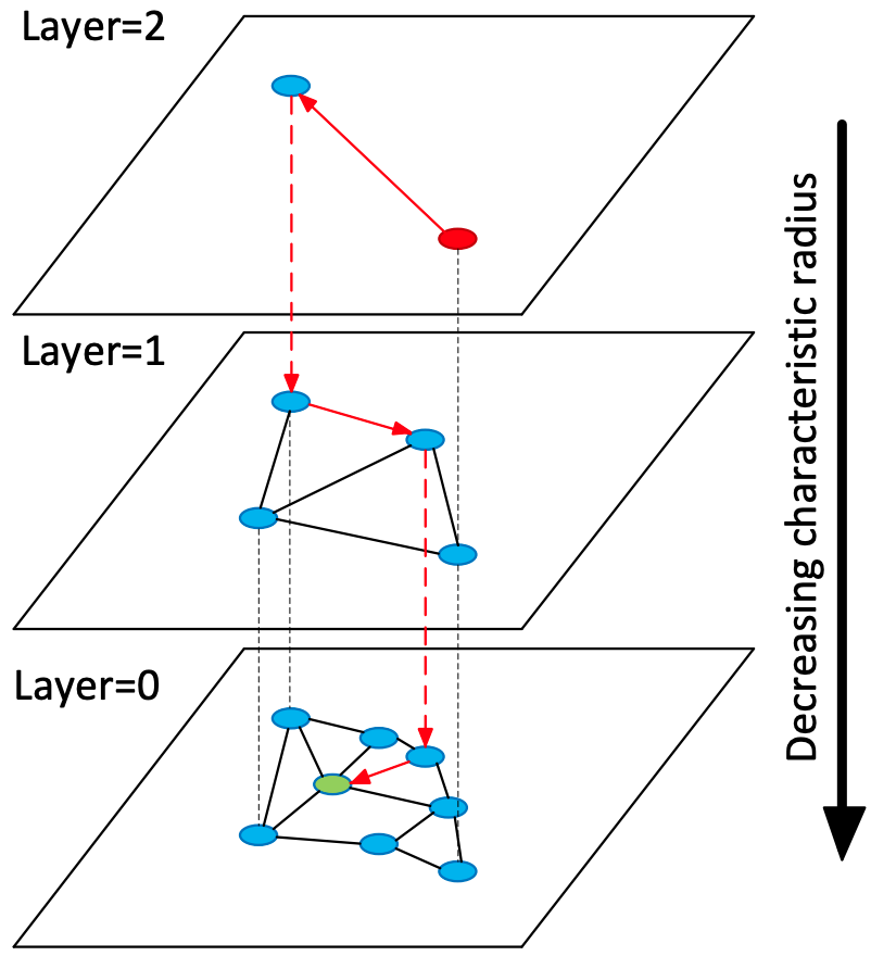
Figure 1. HNSW Index (replicated from reference (Malkov and Yashunin, 2020)).

⬇

1Input: dataset V, efConstruction, M

2Output: HNSW index graph G

3v_e $\leftarrow$ first element of V

4G $\leftarrow$ v_e

5maxLevel $\leftarrow$ randomLevel(v_e)

6for each element v in V \ {v_e}:

7 L(v) $\leftarrow$ randomLevel(v)

8 currEP $\leftarrow$ v_e

9 for ($ly\in maxLeveltoL(v)+1$):

10 currEP $\leftarrow$ GreedySearch(v, currEP, 1, $ly$)

11 for ($ly\in min(maxLevel,L(v))to0$):

12 candidates $\leftarrow$ SearchLayer(v, currEntry, efConstruction, $ly$)

13 selectedNeighbors $\leftarrow$ SelectNeighbors(v, candidates, M)

14 // Prune if more than M neighbors are found

15 if (|selectedNeighbors| > M):

16 selectedNeighbors $\leftarrow$ RNGShrink(selectedNeighbors, M)

17 // Add forward edges and shrink

18 AddEdgesAndShrink(G, v, selectedNeighbors, $ly$)

19 for each neighbor n in selectedNeighbors:

20 // Add backward edges and shrink

21 AddEdgesAndShrink(G, n, v, $ly$)

22 if L(v) > maxLevel:

23 v_e $\leftarrow$ v

24 maxLevel $\leftarrow$ L(v)

25return G

Listing 1: HNSW index creation algorithm

⬇

1Input: Query vector $v_{q}$, $k$, entry point $v_{e}$, candidate size $efs$

2Output: $k$ nearest vectors

3min priority queue $C$ $\leftarrow$ {$v_{e}$} // candidates

4max priority queue $R$ $\leftarrow$ {$v_{e}$} // results

5visited set V $\leftarrow$ {$v_{e}$}

6while(C $\neq$ $\emptyset$):

7 $c_{\text{min}}$ $\leftarrow$ Pop-Min($C$)

8 $r_{\text{max}}$ $\leftarrow$ $|R|<efs$ ? Peek-Max($R$) : $\infty$

9 if ($d(v_{q},c_{\text{min}})>d(v_{q},r_{\text{max}})$): break; // convergence criterion

10 for ($n\in neighbours(c_{\text{min}},l)$): // neighbors in layer l

11 if ($n\notin V$):

12 $V\leftarrow V\cup\{n\}$

13 if ($|R|<efs$ OR $d(v_{q},n)<d(v_{q},r_{\text{max}})$):

14 Insert($C$, $n$)

15 Insert($R$, $n$)

16 if ($|R|>efs$): Pop-Max($R$)

17return closest $k$ vectors in $R$

Listing 2: HNSW search algorithm in a partilar layer $l$.

HNSW search algorithm performs a depth-first search-like traversal algorithm in each level of the index. Algorithm 2 shows the pseudocode of the search in a particular level. The inputs are $v_{q}$, $k$, an entry vector $v_{e}$, and an $efs$ value (explained momentarily). The output is the approximate $k$ NNs of $v_{q}$ in a particular level. The algorithm uses two priority queues: (i) a min priority queue of candidates, which represent vectors whose neighbors have not been explored; and (ii) a max priority queue of results, which store the $efs$ closest vectors seen so far. At each iteration, the algorithm iteratively explores the closest candidates’ neighbors ($c_{min}$ in Algorithm 2) on line 10, starting from $v_{e}$. For each neighbor $n$, if $n$ has not been visited already, $dist(v_{q},n)$ is computed and put into the candidates queue. If $dist(v_{q},n)$ improves the closest vectors seen so far, it is also put into results. The iterations stop when a $c_{min}$ has a distance larger than the $efs$’th closest vector in results (line 9). The algorithm returns the $k$ closest vectors in results.

The full algorithm uses this subroutine at each level, starting from the top level index. At each level $i+1$ except the lowest level, it sets $k=1$ and $efs=1$ to find the closest neighbor $v_{ei}$ of $v_{q}$, which is used as an entry point for the search at level $i$. At the very top level the search starts from a fixed entry point $v_{e}^{*}$. At the lowest level, the algorithm finds $k$ NNs using some $efs$ value greater or equal to $k$. The $efs$ parameter controls the trade-off between search accuracy and latency. The higher the $efs$ value, the longer it will take for the search to converge, but since a larger candidate set is considered, the higher will be the recall.

In HNSW search algorithm the dominant cost is the distance computations, which require expensive floating point operations on vectors. The distance computations are done when a neighbor $w$ of a $c_{min}$ is explored and put into the candidates queue. When we will discuss modified versions of this search algorithm, we will focus on minimizing the distance calculations.

Figure 2. Very low selectivity $S$ can disconnect HNSW.

2.2. Predicate Agnostic Search & Prefiltering

We briefly discuss the challenge of predicate-agnostic vector search, which is the problem of finding kNNs of $v_{Q}$ over an arbitrary subset $S$ of the vectors, that are selected by a selection subquery $Q_{S}$. In this paper we focus on the prefiltering approach to evaluate predicate-agnostic search. In this approach, the system first evaluates $Q_{S}$ and computes $S$. Then, the entire $S$ is passed to the HNSW search algorithm which finds the approximate $k$ nearest neighbors of $v_{Q}$ in $S$. This is the approach adopted by some other systems, such as Weaviate (Weaviate, 2024a) and Acorn (Patel et al., 2024). The core challenge of prefiltering is that the search is performed on $G_{H}$, which was constructed by iteratively connecting each vector $v$ with their closest $M$ neighbors in $V$ and not $S$. As a result $v$’s neighbors in $G_{H}$ that are actually in $S$ can be very sparse or $v$ can even be disconnected from other vectors in $S$. Figure 2 shows this problem pictorially.

2.3. Kuzu Overview

Kuzu (Feng et al., 2023) is a GDBMS that adopts many of the architectural principles of analytical DBMSs, such as adopting disk-based columnar storage structures to store the node and relationship records, vectorized query processor (Abadi et al., 2012), and morsel-driven multi-core parallelism. We refer readers to references (Feng et al., 2023; Gupta et al., 2021) for a detailed description of Kuzu’s design. Here we provide background on the components that are needed to explain the design and implementation of NaviX. Other background is provided in Section 4 when describing different components.

2.3.1. Storage Structures

Node records in Kuzu are stored using a native design that is based on other columnar designs such as Parquet (Parquet, [n.d.]). The storage of relationship records are stored in disk-based compressed sparse row (CSR) structures. This is a highly optimized persistent graph topology design and an example advantage of leveraging the existing capabilities of GDBMSs to implement HNSW-based vector indices.

2.3.2. Node Semimasks

Query plans in Kuzu are composed into several subplans $SP_{1},...,SP_{t}$. Subplans form a directed acyclic graph and are executed one after another. Outputs of one subplan is consumed by the next subplan. Kuzu frequently uses sideways information passing (SIP) by passing node semimasks from one subplan $SP_{i}$ to another $SP_{j}$. Node semimasks identify a subset of the nodes whose properties or relationships need to be scanned in $SP_{j}$. As we describe in Section 4.2, we use node semimasks to pass the results of selection subquery $Q_{S}$ to the subplan that contains the vector search operator.

3. Filtered Search Heuristics

We begin by describing our predicate-agnostic filtered search heuristics. The primary advantage of prefiltering is that because it pays the upfront cost of computing $Q_{S}$ entirely, it has full information about which vectors are in $S$. This information can be utilized during kNN search algorithm. In contrast, post-filtering approaches perform the search without any information about what is in $S$. We next discuss the question of how to use $S$ to design a robust prefiltering algorithm that performs the search efficiently across different selectivity levels and correlation scenarios. Throughout this section, we will discuss several existing search heuristics as well as new ones we introduce. For reference, Table 1 summarizes these heuristics.

Heuristics	Description	Suitable Selectivity
onehop-s	One Hop & only unfiltered nodes	High
directed	Two Hops up to M in optimal direction	Medium to Low
blind	Two Hops up to M in random direction	Very Low
adaptive-global	Use global selectivity to adapt	All (Uncorrelated)
adaptive-local	Use local selectivity to adapt	All (Uncorrelated & Correlated)

Table 1. Summary of search heuristics.

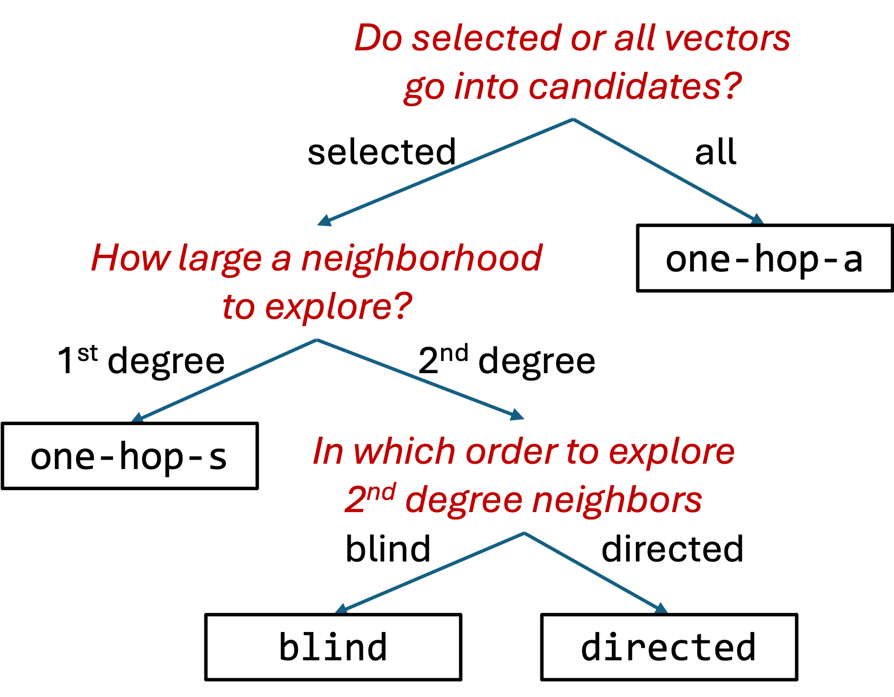
Figure 3. Space of heuristics in a modified search algorithm.

3.1. Design Space of Fixed Heuristics

We begin by outlining a set of fixed heuristic decisions a modified HNSW search algorithm can make and discuss the intuitions of the pros and cons of each. For reference, Figure 3 shows the decision tree that summarizes the space of heuristics we discuss. We emphasize that the core step of the original HNSW search algorithm is that at each iteration, the algorithm explores the closest neighbors of a $c_{min}$ in $V$. Therefore we are interested in developing modified search algorithms that efficiently explore the closest neighbors of a $c_{min}$ in $S$. Intuitively, heuristics that achieve this primary goal should perform the search more efficiently than others.

The first decision is if all or only selected (or unfiltered) vectors should be put into candidates queue. The unmodified HNSW algorithm puts all vectors, which may be inefficient due to exploring unselected vectors. Further, exploring unselected vectors can misdirect the search away from regions that contain selected vectors, slowing down convergence. We refer to the original unmodified HNSW as the onehop-a heuristic (for one hop all vectors). An algorithm can instead decide to explore only selected vectors. We refer to this heuristic as onehop-s. Intuitively onehop-s would improve the convergence of onehop-a at high selectivity levels but creates a separate problem. Specifically, at low selectivity levels the selected projection of $G_{H}$, i.e., the subgraph that contains $S$ and their edges, can be disconnected. Recall Figure 2, which shows this problem pictorially.

The second decision is how much of each candidate’s neighborhood to explore in the original index $G$. To address the disconnected graph problem at lower selectivity levels, an algorithm can explore higher degree neighbors of each candidate. Specifically an algorithm can explore 2nd degree nodes, which we show is adequate in our evaluations. A version of this heuristic has been explored in ACORN (Patel et al., 2024). Given a candidate $c_{min}$ and its neighbors $n_{1},...,n_{\ell}$, ACORN’s heuristic takes the first neighbor $n_{1}$ of $c_{min}$ and explores the selected vectors among $n_{1}$ and $n_{1}$’s neighbors $n_{11},...,n_{1k}$. This is then repeated for the second neighbor $n_{2}$ of $c_{min}$, until $M$ many selected vectors are explored. We refer to this as the blind 2nd degree heuristic (blind for short). We note that in our evaluations, we implement and evaluate an improved version of this heuristic than the one used in reference (Patel et al., 2024). Specifically, we first explore all 1st degree neighbors $n_{1},...,n_{\ell}$ and then start exploring 2nd degree neighbors. This modified version performs strictly better.

The third decision is the order in which the 2nd degree neighbors are explored. The blind heuristic is oblivious to how close each 2nd degree neighborhood it explores is to $v_{Q}$. In other words, it does not perform its exploration in a directed manner towards the regions that are closer to $v_{Q}$. Alternatively we propose exploring the neighbors of $c_{min}$ in increasing order of their distance to $v_{Q}$. Let $n_{1}^{*},...,n_{\ell}^{*}$ be the 1st degree neighbors of $c_{min}$ ordered from closest to $v_{Q}$ to furthest. We refer to the heuristic that explores the 2nd degree neighbors of $c_{min}$ in this order as the directed 2nd degree heuristic (or directed for short). directed has the advantage of prioritizing the search towards regions that are closer to $v_{Q}$ but incurs the cost of computing the distances to each 1st degree neighbor of $c_{min}$.

Within this space, different heuristics have different advantages in different selectivity regions. At high selectivity levels, we expect onehop-s, which limits explorations to selected 1st degree vectors to work well because there is enough selected vectors in $S$ that these heuristics should achieve the primary goal we articulated above. As selectivity decreases and fewer 1st degree neighbors are selected, onehop-s should degrade in recall. Therefore, heuristics that explore 2nd degree neighbors, such as blind and directed should work better. Between these two, directed should converge faster if we focus on the number of candidates it explores. However, directed incurs the additional cost of computing the distance of $v_{Q}$ to every 1st degree neighbor (selected or unselected) of $c_{min}$. The benefits of directed can overweigh its overheads at medium to slightly low selectivity levels. Eventually however, as selectivity decreases enough, directed cannot have an advantage over blind. This is because at low-enough selectivity levels, there is not enough selected nodes even in the 2nd degree neighbors of $c_{min}$. Therefore both directed and blind effectively explore the same set of selected vectors, yet blind does not incur the overhead of computing the distances to unselected 1st degree vectors.

3.2. Adaptive Algorithms

We next describe two adaptive algorithms that utilize the selectivity information in $S$ to pick the best of all worlds across blind, directed, and onehop-s. We first pick an upper bound threshold $ub_{onehop-s}$ above which we pick onehop-s. We found 50% to be a safe choice here although in some of our evaluations slightly lower thresholds also work. To decide between blind and directed, we use the following formula. Recall that under low-enough selectivity, if there are less than $M$ selected vectors in the 1st and 2nd degree neighbors of $c_{min}$, directed has no particular advantage over blind. So it is guaranteed to be suboptimal. Therefore, we try to estimate if we are in this safe region.

Specifically, we calculate the estimated number of selected vectors ($esv$) in the 1st and 2nd degree neighbors of $c_{min}$ with the formula: $esv=\sigma\times(M+1)\times M$, Let $\sigma$ be the selectivity of $S$ (more on this later). The formula multiplies the selectivity with the total sizes of the 1st and 2nd degree neighbors of $c_{min}$. If $esn$ is less than $M$, which is the maximum number of selected nodes blind explores, then directed cannot have an advantage over blind by calculating the distances to each 1st degree node. Therefore we default to blind. This safe region is conservative, so in our implementation we are more lenient and compare $esn$ with $M$*$lf$, where $lf$ (3 by default) is a leniency factor. Figure 4 pictorially shows the regions where we hypothesize each fixed heuristic to work well.

Figure 4. Optimal selectivity regions of fixed heuristics.

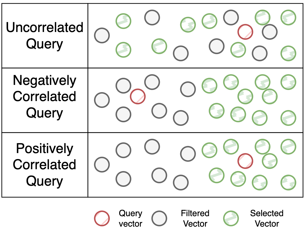
Figure 5. Pictorial depiction of different correlations $S$ can have with $v_{Q}$’s neighborhood. Replicated from reference (Patel et al., 2024).

We can configure the above adaptive algorithms in two different ways. First, we can use the global selectivity of $S$ as $\sigma$, $\sigma_{g}=|S|/|V|$. We refer to this version of the algorithm as adaptive-global (adaptive-g for short). As we demonstrate in our evaluations, this algorithm is able to capture the best of all worlds. However, we can improve this algorithm, and even any fixed-heuristic in their optimal regions, by choosing a possibly different heuristic for each candidate $c_{min}$. This is useful if $S$ correlates with certain regions in $G$ and is not a random subset of $V$. Figure 5 pictorially shows the three different possibilities of $S$ being uncorrelated, positively, or negatively correlated with the region around $v_{Q}$. Especially in correlated scenarios, even though the global selectivity of $S$ is low enough and we are in the optimal selectivity region for the blind heuristic, if $c_{min}$ is in a region that contains more selected vectors, it might be better to choose onehop-s heuristic for $c_{min}$.

We refer to the adaptive algorithm that uses the local selectivity of $c_{min}$ during each search iteration to pick a heuristic as adaptive-local. Specifically, adaptive-local uses $\sigma_{l}=$
$|S(nbrs(c_{min}))|/|nbrs(c_{min})|$, where $nbrs$ $(c_{min})$ is the neighbors of $c_{min}$ and $S(nbrs(c_{min}))$ is the selected neighbors of $c_{min}$. $\sigma_{l}$ calculates the fraction of $c_{min}$’s neighbors that are selected. Note that $\sigma_{l}$ is computed merely by checking if each neighbor of $c_{min}$ in $S$. In our implementation, this is done by checking the bits of these neighbors in a Kuzu node mask (see Section 4). Importantly, this operation does not require any filtering or distance computations. Finally, Table 1 presents the summary of these heuristics.

In this paper, we propose adaptive-local as a predicate-agnostic filtered search algorithm and demonstrate that it is efficient under both different selectivity levels and correlation scenarios.

4. Implementation Details

We next describe the design and implementation of NaviX in Kuzu.

4.1. Index Creation

Index creation is executed as a standalone CALL function in Cypher. Suppose there is a node table with schema ‘Chunk(id UINT64, docID UINT64, embedding FLOAT[1024])’. Below is an example query creating an index called ChunkHNSWIndex on the embedding property of Chunk nodes.

⬇

1CALL CREATE_HNSW_INDEX(’ChunksHNSWIndex’, ’Chunks’, ’embedding’, M_U)

NaviX is a 2-level HNSW implementation. $M_{U}$ is the maximum degree of vectors in the lower level index. During construction, two in-memory CSR data structures $G_{L}$ (for lower level) and $G_{U}$ (for upper level) are initiated. The sizes of these CSRs are respectively, $n$ and $n*s$, where $n$ is the number of nodes in the indexed node table and $s$ is sampling rate for $G_{U}$ (by default 5%). $G_{U}$ and $G_{L}$ are initiated with $M_{U}$ and $M_{L}=M_{U}*2$ pre-allocated edges for each node. Each worker thread concurrently scans a morsel of vectors (2048 many) from disk and updates the shared CSR structures using the HNSW construction algorithm from Section 2. Note that as a thread $T_{i}$ updates these CSRs, other threads might be modified by other threads as well. However HNSW is already an approximate index and our evaluations demonstrate that the index quality can tolerate this possible data race. So, we recommend this optimization to obtain better parallelism during construction. We note that while $G_{U}$ and $G_{L}$ are kept in memory during construction, all accesses to the vectors, which are much larger than $G_{U}$ and $G_{L}$, happen through the buffer manager. For example, on our Wiki dataset, vectors take 63GB while the lower level of the index only takes 7.8GB.

Once $G_{L}$ is contructed, we pass it to Kuzu’s CSR construction pipeline. $G_{U}$ could also be persisted using Kuzu’s existing disk-based structure. However, because it is intended to be very small, we persist it using a simpler format that writes the offsets and edges consecutively on disk.

Observe that as per our first design goal, we leverage many of the existing capabilities of the underlying GDBMS, including its storage structures, which are automatically compressed on disk by Kuzu, its automatic query parallelization mechanism, and many of its operators, such as scans, Node Masker (next subsection), and CSR Construct. We did not modify any of these core components. This is an important advantage that simplifies the engineering efforts of system developers. From a performance point of view, leveraging Kuzu’s existing capabilities has both performance advantages and disadvantages. For example, Kuzu’s CSR indices are automatically bit compressed and its semimask creation pipeline is well optimized. Furthermore, by storing vectors and the index (i.e., the adjacency lists) separately, a buffer manager can pack multiple adjacency lists in a single 4KB page. This constrasts with other designs, such as DiskANN (Subramanya et al., 2019), which packs the actual vector and the adjacency list of a vector in a page and caches compressed versions of the vectors in memory. Our design helps in caching more adjacency lists with less amount of memory through the buffer manager. However, at the same time all adjacency list accesses in Kuzu perform two buffer manager (and possibly I/O if not cached) operations: one to read some metadata and the other to read the actual list. Instead, more specialized designs can do other optimizations that are not implemented in the underlying GDBMS. For example, DiskANN performs a single IO to access both the actual vector and its adjacency list.

4.2. Index Search Query Syntax and Plan

To describe the index search query syntax, we replicate our query from Section 1:

⬇

1MATCH (a:Person)-[:Mentions]->(b:Chunk)

2WHERE a.name = "Alice"

3PROJECT GRAPH AliceNodes (b);

4CALL QUERY_HNSW_INDEX(AliceGraph, ’ChunkHNSWIndex’, k=100,

5 q=[0.1, 0.4, ..., 0.8])

6RETURN q, b, _rank

Here, $Q_{S}$ is the subquery specified by the MATCH and WHERE clauses and identify the Chunk nodes that are mentioned by a Person with name Alice. The PROJECT GRAPH clause is used to identify the selected vectors $S$ that will be passed to QUERY_HNSW_INDEX function. Figure 6 shows the plan structure for evaluating predicate-agnostic search queries. The first subplan evaluates $Q_{S}$ and uses Kuzu’s Node-Masker operator to create a node semimask. This is then passed to the second subplan that starts with an HNSW Search operator that takes in the semimask and runs a modified HNSW algorithm. We note that during HNSW Search computation, no filtering is done. All filtering is performed apriori in the subplan that evaluates $Q_{S}$. All accesses to the persisted adjacency lists of vectors ($G_{L}$) in the index and to the actual vectors happen through the buffer manager of the system. The upper layer $G_{U}$, however, remains in memory at all times since it is extremely small compared to the complete index (including vectors). For instance, in our Wiki dataset, $G_{U}$ occupies only $\sim$200MB while the full index including vectors requires $\sim$70.8GB.

4.2.1. In-Buffer Manager Distance Computations

We end this section with an optimization that may be of interest to system developers. As we discussed above, during both index construction and search, vectors are scanned through the buffer manager to improve the scalability of NaviX. In the standard approach in DBMSs, each piece of data is first copied from the buffer manager’s frames to an operator-local buffer. Then, the operator operates on this data. We observed that the copy operations are a performance bottleneck. To address this, we extended the storage manager interfaces of Kuzu to directly run a function on the data residing in buffer manager frames without performing any copies. Specifically, we pass a distance function to the buffer manager. The buffer manager finds and pins a frame, if necessary, scans the vector from disk to the frame, runs the function, and unpins the frame. In Appendix A.3 we show that this optimization can improve vector search latencies by up to 1.6x. Finally, we used the SimSIMD (Vardanian, [n.d.]a) library to perform distance computations using SIMD instructions.

Figure 6. NaviX search plan.

5. Evaluation

We next evaluate the performance of NaviX, which refers to our implementation that uses the adaptive-local search algorithm.

5.1. Experimental Setup

5.1.1. Baselines

We used the following baseline systems:

Kuzu configurations: We implemented our different heuristics in Kuzu: (i) Kuzu-onehop-s; (ii) Kuzu-blind; (iii) Kuzu-directed; (iv) Kuzu-ag, which adopts the adaptive-g heuristic; and (v) NaviX, which adopts the adaptive-local heuristic.

ACORN (Patel et al., 2024) and FAISS-Navix: ACORN is a proximity graph implementation that supports predicate-agnostic vector search using a modification of the blind heuristic. ACORN is an in-memory implementation on top of the FAISS system (Meta, 2018a). We implement our adaptive-local heuristic also on top of FAISS to compare against ACORN, which we refer to as FAISS-Navix.

Weaviate (v1.28.2) (Weaviate, 2024b) and Milvus (v2.5.0) (Milvus, 2024): These systems serve as baselines of specialized vector databases. Weaviate also serves as baselines of an external implementation of some of the prefiltering heuristics we covered. Milvus instead performs a mix of pre- and postfiltering evaluation depending on the selectivities.

DiskANN (Subramanya et al., 2019) and FilteredDiskANN (Gollapudi et al., 2023): DisANN is a disk-based vector index implementation that performs I/O when scanning adjacency lists of candidate vectors. FilteredDiskANN is an enhancement of DiskANN that support a limited set of filters.

iRangeGraph (Xu et al., 2024b): Similar to FilteredDiskANN, iRangeGraph supports filtered vector search queries in a “predicate-conscious” manner. That is, it modifies its index apriori to support limited range queries. However, it is more efficient than FilteredDiskANN and is an in-memory implementation.

PGVectorscale (v0.5.1) (Timescale, 2024) and VBase (Zhang et al., 2023): These systems are two vector index implementations on Postgres that serve as baselines of vector indices that are implemented inside an existing DBMS. They also serve as baselines that implement postfiltering approaches.

Note on brute force search: Except for VBase, at very low selectivity levels, our baselines adopt the brute-force heuristic, which computes distances to every vector in $S$ and returns the kNNs with 100% accuracy. This will be relevant in our experiments in Section 5.4.

Dataset	# Vectors	Dimension	Distance Fn
GIST (Jegou et al., 2011)	1M	960	L2
Tiny (Li et al., 2018)	5M	384	L2
Arxiv (Qdrant, [n.d.])	2.1M	384	Cosine
Wiki	15.4M	1024	Cosine

Table 2. Datasets

5.1.2. Datasets

We used the four datasets in Table 2.

GIST, Tiny, and Arxiv: GIST and Tiny are two datasets that contains embeddings of images that have been embedded using local GIST descriptors (Oliva and Torralba, 2001), which is a feature representation technique for images. GIST uses local INRIA Holidays images (Jegou et al., 2008) and Tiny contains images from the TinyImages dataset (Torralba et al., 2008). Arxiv is a recent open-source dataset that embeds titles from the arXiv (arXiv, [n.d.]) paper dataset using the all-MiniLM-L6-v2 (Transformers, [n.d.]) text embedding model.

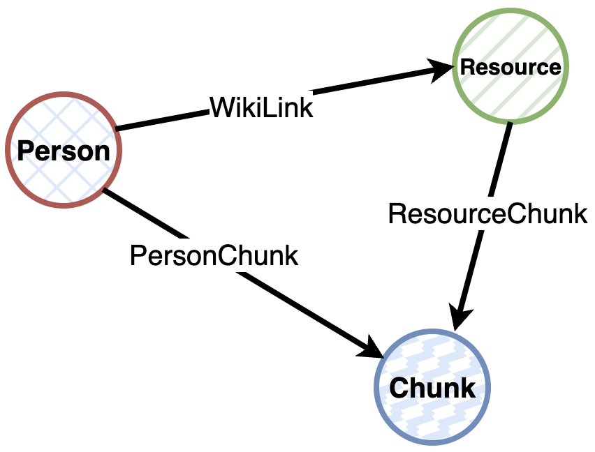
(a) Property Graph Schema

(b) Relational Schema

Figure 7. Wiki Schema

Wiki: The above datasets contain objects but no connections between objects. Therefore we can use them with predicate-agnostic queries where the selection subqueries contain simple filters but not joins. Moreover, these filters are uncorrelated with the query vectors (see Section 5.1.3). To extend our evaluation to selection subqueries with joins and different correlations, we prepared a new dataset from DBPedia latest version (DBpedia, 2024) and the Wikipedia dump (WikiMedia, 2024). DBPedia is an RDF graph of (subject, predicate, object) triples. The dataset schema is shown in Figures 7(a) and 7(b) both as a property graph and a relational database.

• Person(pID) nodes: We modeled each resource with a dbo:birthPlace and dbo:birthDate predicate as a Person.

• Resource(rID) nodes: In the DBPedia graph, we do a 2-hop traversal around Persons along the dbo:wikiPageWikiLink predicates and model each resource we visit as a Resource node.

• Chunk(cID, embd) nodes: We chunked the Wikipedia articles of each Person and Resource node into 1028 tokens and created a Chunk node. We embedded each chunk into 1024 dimensional vectors using the stella_en_400M_v5 (Search, 2024) model on Hugging Face (HuggingFace, [n.d.]) and stored it as an embedding property.

• PersonChunk, ResourceChunk, and WikiLink relationships: We connected each Person and Resource to the Chunk nodes of their corresponding Wikipedia articles, respectively, as PersonChunk and ResourceChunk relationships. We also added WikiLink relationships from Person nodes to their first degree Resource nodes.

Correlation	Query	Filter
Uncorrelated	Where is Amazon located?	Random filtering on Chunks
Positively Correlated	Which company did Jeff Bezos start?	Chunks of person nodes
Negatively Correlated	Where is the Eiffel Tower located?	Chunks of person nodes

Table 3. Examples of Correlated Queries in Wiki Dataset

Selectivity	90%	75%	50%	40%	30%	20%	10%	5%	3%	1%
Wiki	0.98	0.98	0.98	0.98	0.99	0.98	1.00	1.02	1.12	1.12
Tiny	1.00	1.00	1.00	1.00	0.98	0.99	1.02	1.00	0.98	0.90
Arxiv	0.99	0.99	1.03	1.05	1.06	1.07	1.10	1.10	1.12	1.14
GIST	0.90	0.99	0.99	1.00	1.01	1.01	1.01	0.96	1.04	1.18

Table 4. Correlation ratios of uncorrelated workloads.

Correlation	Negatively Correlated					Positively Correlated
Selectivity	22.9%	15%	9.9%	5.1%	1%	22.9%	15%	9.9%	5.1%	1%
Wiki	0.055	0.050	0.055	0.064	0.037	2.65	2.90	2.64	2.57	2.90

Table 5. Correlation ratios of for Wiki negatively and positively correlated workloads.

5.1.3. Query Workloads

Our main workloads contain predicate-agnostic queries on our datasets. Each query $Q$ consists of two main components: (i) $Q_{S}$ is a selection subquery that selects a subset $|S|$ of the vectors from the entire indexed vectors $V$; and (ii) $v_{Q}$ is a query vector. $Q$ finds kNNs of $v_{Q}$ within $S$. We refer to the global selectivity of $Q_{S}$ as $\sigma=|S|/|V|$. In each $Q$, $v_{q}$ can be “uncorrelated”, “positively”, or “negatively” correlated with $S$, which we define as follows. Let $\text{knn}^{v_{Q}}_{V}$ be the kNNs of $v_{Q}$ in $V$. Let $\text{knn}^{v_{Q}}_{S}\subseteq\text{knn}^{v_{Q}}_{V}$ be the subset of these neighbors that are in $S$. We use $\sigma_{v_{q}}=\text{knn}^{v_{Q}}_{S}/\text{knn}^{v_{Q}}_{V}$ as a metric for the selectivity of $v_{Q}$’s kNNs in $V$. Our correlation metric measures if $\sigma_{v_{q}}$ and $\sigma$ are correlated:

$$\text{ce}=\sigma_{v_{q}}/\sigma$$

If ce $\approx$ 1, then $v_{Q}$ is uncorrelated with $S$. If ce $\gg$ 1 (ce $\ll$ 1), then $v_{Q}$ is positively (negatively) correlated with $S$, as the neighbors of $v_{Q}$ are more (less) likely to be in $S$ than a random node.

Uncorrelated Workloads: For each dataset, our uncorrelated queries have a $Q_{S}$ that filter embedded objects on their IDs:

⬇

1MATCH (c:Chunk) WHERE c.cid < (MAX_CHUNK_ID * $\sigma$)

2PROJECT GRAPH S(c);

3CALL QUERY_HNSW_INDEX(S, HNSWIndex, v_Q, k) RETURN c.cID;

We populate this template with different $\sigma$, $v_{Q}$, and $k$. For GIST, Tiny, and Arxiv, we randomly selected 50 queries from their own query sets. For Wiki, we generated 50 queries for uncorrelated and positively correlated cases as follows. We chose a random Person node $p$, sampled its chunks and chunks of connected Resource nodes, and used OpenAI’s o1 model (OpenAI, [n.d.]) to generate questions about $p$ using these chunks as context. We provided chunks until reaching the 128K token limit. We embedded o1’s question as $v_{Q}$ also using stella_en_400M_v5. To get an uncorrelated $S$, we selected Chunks based solely on chunkIDs as in the above Cypher query, which filters chunks uniformly.

Wiki Positively Correlated Workload: We used the same $v_{Q}$’s of the uncorrelated Wiki workload but changed $Q_{S}$ as follows:

⬇

1MATCH (p:Person)-[e:PersonChunk]->(c:Chunk)

2WHERE p.birth_date >= {s_date} AND p.birth_date < {e_date}

3PROJECT GRAPH S(c)

4CALL QUERY_HNSW_INDEX(S, HNSWIndex, v_Q, k) RETURN c.cID;

The selection subqueries are 1-hop queries that select a subset of Person nodes based on their birthdates, which we expect are more likely to be in the neighborhood of $v_{Q}$’s than a random Chunk.

Wiki Negatively Correlated Workload: For $Q_{S}$, we use the 1-hop selection subqueries that select Chunks of Person nodes. For $v_{Q}$ we prompt $o1$ to generate questions about non-people entities, such as cities, monuments, and companies.

Table 3 shows an example of natural language queries for each correlation scenario. Tables 4 and  5 report the average correlations (ce) of these queries for different selectivity levels and correlated scenarios. Note that our selectivity levels go up to 100% in uncorrelated workloads as we can use predicates that select every object. For Wiki correlated workloads, selectivities are at most 22.9% because the 1-hop queries select Chunks that come from articles of Person nodes, which constitute 22.9% of all Chunks.

5.1.4. Evaluation Metric

For most experiments, we measure baseline latency on a dataset/workload under varying selectivity levels when searching for the $k$=100 nearest neighbors of $v_{Q}$. Since kNN is approximate, our main experiments target 95% recall and adjust the efs parameter to stay within 1% of it. If a baseline gives higher recall than 95% with the minimum efs value, then we match that for all other baselines. If a baseline fails to reach 95% recall even at efs 1000, we mark that point with a cross sign in our figures. VBase does not have any knobs to tune its recall, so we use it in its default configuration.

Systems	GIST 1M	Arxiv 2.1M	Tiny 5M	Wiki 15.4M
PGVectorScale	336.34	456.63	3153.52	5932.81
VBase	54.84	71.32	294.12	942.78
Weaviate	19.14	22.80	57.44	187.65
Milvus	19.85	23.66	50.15	182.42
DiskANN	NA	NA	NA	130.78
FilteredDiskANN	NA	NA	NA	142.89
iRangeGraph	NA	40.90	162.42	NA
ACORN-1	1.69	1.75	4.99	23.85
ACORN-10	11.55	10.97	38.55	162.66
FAISS-Navix	3.29	3.78	12.22	42.05
NaviX	5.13	7.09	18.25	55.22

Table 6. Indexing Time (mins). All systems use 32 threads except for PGVectorScale and VBase, which are single threaded.

5.1.5. Index Configurations

We built the HNSW indices with maximum connection $M$ parameter set to 32 in upper layers and 64 in lowest layer and $efC$ set to 200 across all systems. Similarly, we built the other proximity graph-based indices such as DiskANN and ACORN using similar configurations. We used Milvus in its single segment/partitioned configuration as all other baselines and NaviX stores the index in a non-partitioned way. Table 6 reports the index-building times when using 32 threads on our hardware (see below), except PGVectorScale and VBase which have single-threaded index construction implementation. Although our focus is not on index construction time, NaviX’s construction times are always faster than disk-based baselines.

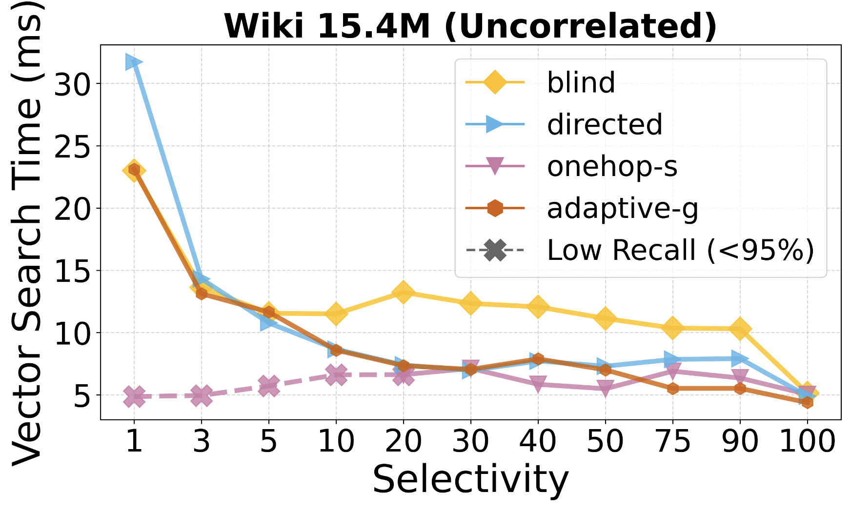
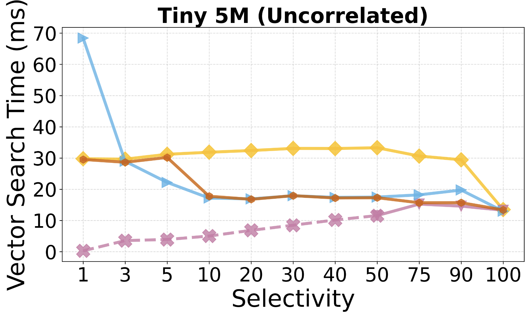
Figure 8. Vector search time vs Selectivity for different heuristics within 95% to 95.5% recall

Figure 9. t-dc vs s-dc of blind and directed.

5.1.6. Index Size and Sampling Ratio

In NaviX  we set the sampling ratio to 5%. This results in a high-level in-memory index size of at most $\sim$200MB (on our largest dataset Wiki). This requirement is a tiny fraction of the storage requirements for vectors and the lower level graph. For example, on Wiki, vectors take $\sim$63GB, while the lower level graph takes $\sim$7.8GB.

5.1.7. Other Experimental Setup Details

Each query workload contains 50 different $v_{Q}$ and all numbers in our experiments are averages across these queries. Except in our disk-based experiments in Section 5.8, for each query $Q$, we first warm up the buffer manager by running $Q$. Then we run each query 5 times and report the average latency of $Q$. Unless otherwise specified, all latency numbers measure end-to-end latency, i.e., including both the time to execute the selection subquery and kNN search. We ran our evaluation on Compute Canada (Canada, [n.d.]) on a single x86 machine with 180 GB of memory and 32 v-CPUs using an Intel(R) Xeon(R) Platinum 8260 processor. Because we could not install DiskANN on this machine, for DiskANN and FilteredDiskANN benchmarks we used a different machine with 132GB of memory, 32 v-CPUs and 2.5T of SSDs.

Figure 10. Vector search time vs selectivity for NaviX and adaptive-g.

Figure 11. Heuristic calls.

5.2. Prefiltering Fixed Heuristics and Adaptive-G

We begin by studying the behaviors of different fixed prefiltering heuristics and adaptive-g. We used each dataset and their uncorrelated workloads. Since each of the Kuzu configurations have the same prefiltering cost for evaluating the selection subqueries, we only report vector search times. Figure 8 presents our results.

First, as hypothesized in Section 3, across all datasets, onehop-s consistently has lower latency than other heuristics as it always limits its distance calculations to only the selected vectors in first degree neighbors of candidates. However, its recall drops significantly below 50% selectivity for Tiny5M and 30% for Wiki (Figure 8). Therefore, above 50% selectivity, onehop-s is the most performant of the fixed heuristics across all datasets.

Second, observe that at very high selectivity levels, blind and directed perform very similarly. This is because at very high selectivity levels, say 100%, since each first degree neighbor is selected, both directed and blind explore only the first degree neighbors. Then as selectivities decrease, directed starts outperforming blind. Once the selectivities are low enough, blind starts outperforming directed.

To explain this behavior, we measured two further metrics. First, we measure the number of distance calculations these heuristics perform across the selected vectors (s-dc). This number is equivalent to the number of vectors a heuristic puts into the candidates priority queue. This is a measure of how effective the search is. Second, we measure the total distance calculations a heuristic makes (t-dc). For blind, t-dc is always equal to s-dc. However, for directed, t-dc can be larger than s-dc as directed computes distances to unselected vectors in the 1st degree neighbors of candidates. We use the difference of t-dc and s-dc as a measure of directed’s overhead. Figures 9 show the s-dc numbers for blind and directed  and t-dc numbers for directed.

As selectivity levels decrease, a larger fraction of the 1st degree neighbors are unselected, so directed’s overhead of computing the distances to them increase. Further, irrespective of the selectivity level, directed performs the search as effectively or better than blind. However, directed’s effectiveness edge over blind is low at very high and very low selectivity levels because at these levels they perform very similar explorations. As we already observed above, at very high selectivity levels these heuristics perform very similar searches. At very low selectivity levels, since very few vectors are selected, both heuristics again behave similarly because both explore every 2nd degree neighbor. That is also why at very low selectivity levels, blind outperforms directed in latency, because directed’s overhead are highest and it does not have an important advantage in terms of its search effectiveness. directed however has an edge over blind at medium selectivity ranges of 50% to 5% where its search edge is larger and overheads are low enough. At roughly these ranges, directed outperforms blind by up to 2x in latency. Overall, between 50% and 5% selectivity, directed is the most performant fixed heuristic. Below and at 5% selectivity, blind outperforms both directed and onehop-s. This matches the regions we outlined in Figure 4.

Next, observe that, except for a few small regions, adaptive-g follows the lowest-latency fixed heuristics in almost all ranges, indicating that using global selectivity information is enough to capture the best of all fixed heuristics. The only exception is within ranges below but close to 50% on some datasets. This is because we choose 50% as a safe threshold in adaptive-g to switch to onehop-s, although in some datasets even between 30% and 50%, onehop-s’s recall is high enough.

5.3. Adaptive-G and NaviX

In our next set of experiments we focus on comparing adaptive-g and NaviX (adaptive-l). Our goal is to show that NaviX is a strict improvement over adaptive-g and the advantage of NaviX is especially visible when queries are correlated. We used the Wiki dataset and each of its workloads and measured the vector search times of adaptive-g and NaviX. We also used the uncorrelated workloads of our datasets. Our observations for these experiments are similar to Wiki uncorrelated dataset and are presented in Appendix A.1.

Figure 10 shows our results. Observe that in the Wiki uncorrelated workload, adaptive-g and NaviX perform very similarly. However in both the negatively and positively correlated cases, the local selectivity of candidate nodes during search can be different than the global selectivity of $S$. Therefore we see adaptive-g and NaviX behaving differently. Overall we observe that NaviX does better decisions and outperforms adaptive-g consistently, in some cases up to a factor of 1.7x. For example in the negatively correlated benchmark at 5% selectivity level, the average vector search latency of adaptive-g is 69.13 ms while that of NaviX is 40.67 ms.

To verify that NaviX and adaptive-g make different choices in terms of the heuristics they pick, we calculated the distribution of each heuristic they pick for different workloads. Figure 11 shows these distributions for the Wiki negatively correlated workload. The figure reports what fraction of times NaviX and adaptive-g picks each heuristic when exploring a candidate’s neighborhoods for each selectivity level. Observe that since adaptive-g’s choice is based on the global selectivity, at each selectivity level, it commits to using one heuristic. Instead, NaviX makes more nuanced decisions. For example, at 22.9% selectivity, while adaptive-g commits to directed, NaviX picks onehop-s 80% of the time, indicating that it has performed the majority of the search in a region that contain vectors with very high local selectivity.

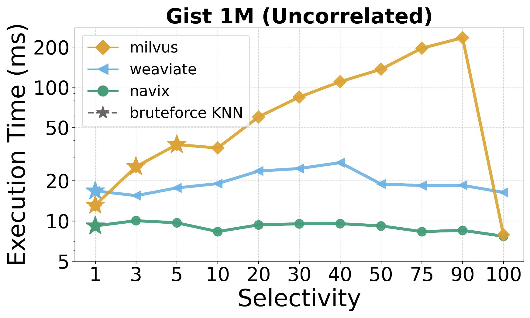
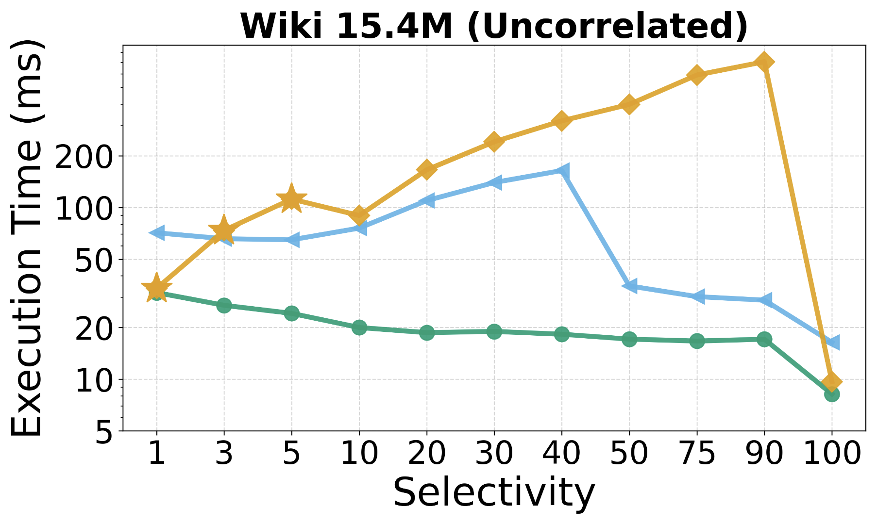
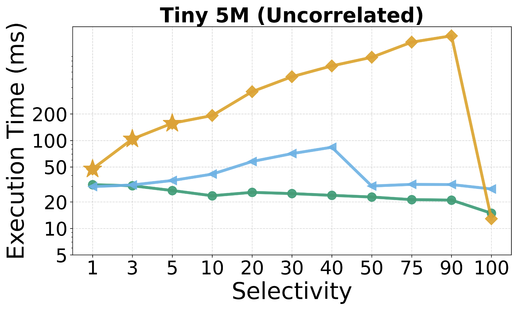
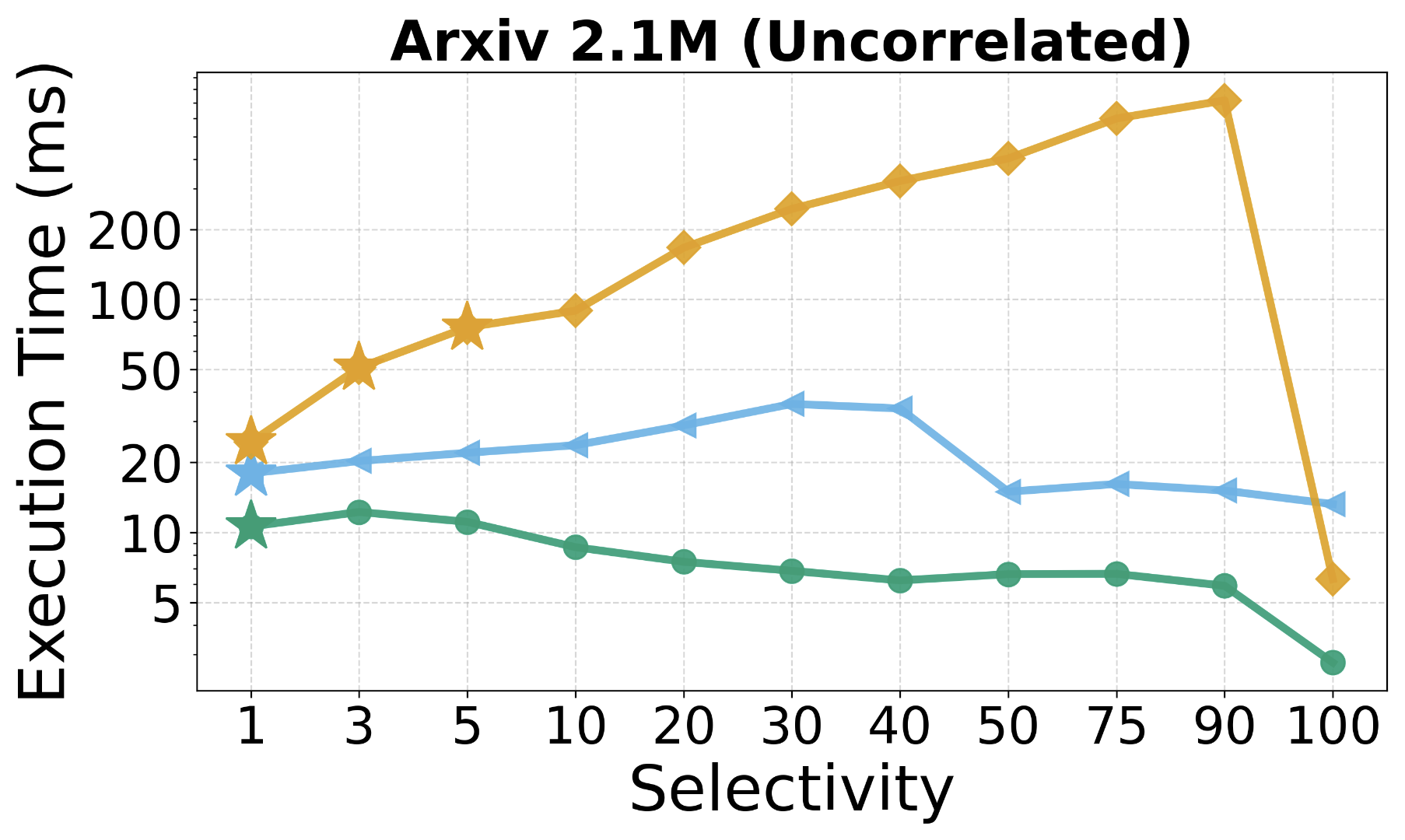
Figure 12. Execution Time vs Selectivity for prefiltering baselines at 95% recall

Figure 13. Vector Search Time vs Selectivity for ACORN and Faiss-Navix baselines at 95% recall

Figure 14. Vector Search Time vs Selectivity for ACORN and Faiss-Navix at different recalls.

Figure 15. Execution Time vs Selectivity for Weaviate and Milvus baselines at different recalls.

	Wiki Uncorrelated					Wiki Negatively Correlated
Selectivity	90%	50%	30%	10%	1%	22.9%	15%	9.9%	5%	1%
Prefiltering	11.28	12.03	11.78	10.64	10.23	32.15	26.27	21.99	18.72	11.76
Vector Search	5.82	5.09	7.20	9.36	22.19	33.71	33.25	39.23	40.67	53.94
Prefiltering %	65%	70%	62%	53%	31%	48%	44%	35%	31%	17%

Table 7. Vector search vs Prefiltering (ms) for Navix.

5.3.1. Prefiltering vs vector search time:

The runtime numbers we presented in Figure 10 focused only on vector search time, since the time spent on prefiltering is same across adaptive-g and NaviX. We next perform a drill-down analyses into how much time is spent by NaviX on prefiltering vs vector search using our largest dataset Wiki. Recall from Section 5.1.3 that our uncorrelated workloads have a simple selection sub-query that puts a range filter on the IDs of embedded objects. In contrast, Wiki correlated workloads have selection sub-queries that contain 1-hop joins from a subset of nodes. This can be more expensive, especially if the selectivities are higher, so the join processes a large number of nodes. Table 7 presents the times spent by NaviX on prefiltering and vector search. We see that on Wiki uncorrelated, the prefiltering time is relatively constant and its contribution to the total execution time decreases as selectivities decrease and vector search becomes more expensive. In contrast, we see that for Wiki negatively correlated, the prefiltering times increase as selectivities increase. This is because the time required to perform the join gets more expensive. However, the contribution of prefiltering to the total time (last row in the table) in both cases decrease as selectivities decrease, and vector search becomes more challenging.

5.4. Weaviate and Milvus

We next compare NaviX against Milvus and Weaviate, which are our disk-based prefiltering baselines. These systems do not support joins, so we compare their behavior only on uncorrelated workloads. Figure 12 shows our results. Weaviate adapts between two search heuristics. Above 40% threshold they use the onehop-a heuristic which explores all selected and unselected nodes. Below and at 40%, they use the simpler version of blind from ACORN (Patel et al., 2024) that is configured to explore between 32 and 8$\times$32 many vectors in the 2nd degree. This explains the latency hikes at 40%. Milvus is overall the slowest system in our experiments. Milvus does onehop-a heuristic at 100% and bruteforce below and at 5% selectivity, where we start observing latency drops. It performs postfiltering at the higher selectivities and onehop-a based prefiltering at the medium to lower selectivities (Wang et al., 2021). Observe further that NaviX outperforms both of these systems. Specifically, when Weaviate switches to blind heuristic at 40% selectivity, the difference is quite drastic, 18.28 ms for NaviX compared to 164.19 ms for Weaviate on Wiki dataset. We attribute these performance differences partly due to NaviX’s better choice of search heuristics and partly to its fast zero-copy distance computations. These experiments indicate that vector indices inside DBMSs can be competitive with specialized vector databases.

We further repeated these experiments to verify that our observations remain the same in other target recall rates. For Wiki and Arxiv, each system we used already achieves our target rate of 95% in the lowest possible efs across most selectivity levels. We therefore increased our target rate to 97%. For GIST and Tiny, we set a target rate of 90%. Figure 15 shows our results for Wiki-uncorrelated and Tiny. The remaining results are shown in Appendix A.5. Observe that the performance patterns of Navix, Milvus, and Weaviate are similar in these datasets as in Figure 12.

5.5. ACORN

We next compare NaviX against ACORN (Patel et al., 2024), which also supports predicate-agnostic vector search on an HNSW-like index. Regardless of the selectivity level, ACORN implements a variant of the blind heuristic on top of the in-memory FAISS HNSW index (Meta, 2018a). ACORN is also configured with a parameter $\delta$, which changes the original index by removing (for $\delta$=$1$) or modifying (for $\delta$ $>$ $1$) the pruning routine during index construction, which makes the graph denser for any fixed $M$ value. Recall that NaviX does not change the underlying HNSW index.

Because ACORN is implemented on top of FAISS, we also implemented adaptive-local on top of FAISS HNSW. We call this version of NaviX as FAISS-Navix. We compare FAISS-Navix against ACORN with $\delta$=$1$ and $\delta$=$10$ using all of our workloads. For $\delta$=$1$, we used $M$=$64$ instead of $M$=$32$ because $M$=$32$ setting was not able to reach our recall rate. This is an important observation: when $\delta$=$1$, ACORN skips the pruning step, which leads to an index with actually more edges than Faiss-Navix ($\sim$1.2x). Therefore the removal of pruning, despite making the HNSW graph denser in fact degrades recall. This indicates the pruning routine is essential for creating diverse edges within proximity graphs. Table 6 shows the indexing times of ACORN and FAISS-NaviX. Observe that ACORN-10 takes significantly more time to build the index as it builds a very dense index. For example, for the Wiki dataset, ACORN-10 takes 3.87x more time compared to Faiss-Navix (162.66 mins vs 42.05 mins).

Figure 13 shows our results on Wiki and Arxiv, and Figure 17 shows our results on GIST and Tiny. Our first observation is that FAISS-Navix consistently outperforms both ACORN configurations and ACORN-10 consistently outperforms ACORN-1. The latter observation is consistent with the observations in reference (Patel et al., 2024). Recall that our previous experiments showed that blind is a good choice in very low selectivity levels but is suboptimal in medium and high selectivity levels. Since ACORN always uses blind, we see that FAISS-Navix outperforms ACORN with bigger margins at higher selectivity levels. For lower selectivity levels, we attribute FAISS-Navix’s superior performance to two advantages it has over ACORN: (i) recall from Section 3.1 that FAISS-Navix’s blind is a strict improvement over ACORN’s blind; and (ii) FAISS-Navix uses the local selectivities to adaptively select heuristics other than blind.

Our second observation is that Faiss-Navix generally outperforms ACORN with larger factors in correlated cases. For example, at around 20-22% selectivity, while Faiss-Navix outperforms Faiss-ACORN-10 and Faiss-ACORN-1, respectively, by factors 1.65x (2.7ms vs 4.44ms) and 5.45x (2.7ms vs 14.72ms), in the negatively correlated case, the differences are 5.31x (10.61ms vs 56.41ms) and 29.29x (10.61ms vs 310.8ms). We also attribute this to Navix’s more advanced search heuristics.

Similar to our experiments with Weaviate and Milvus, we further repeated these experiments at different recall rates. Figure 14 shows our results for Wiki-uncorrelated and Tiny. The remaining results are shown in Appendix A.4. Observe that the performance patterns of FAISS-Navix, ACORN-1, and ACORN-10 are similar in these datasets as in Figure 13 and 17 .

Finally, our FAISS-Navix experiments give a sense of the performance difference between implementing Navix inside a DBMS, where accesses to both neighborhoods of vectors and the actual vectors happen through the buffer manager, vs a completely in-memory HNSW implementation. Specifically, we can compare the Wiki runtimes in Figure 10 and 13, which use the same workloads. For example, on the Wiki-uncorrelated benchmark, the runtimes of Navix in Kuzu change between 4.5-22.19ms, while in FAISS, the runtimes are between 2.02-7.74ms.

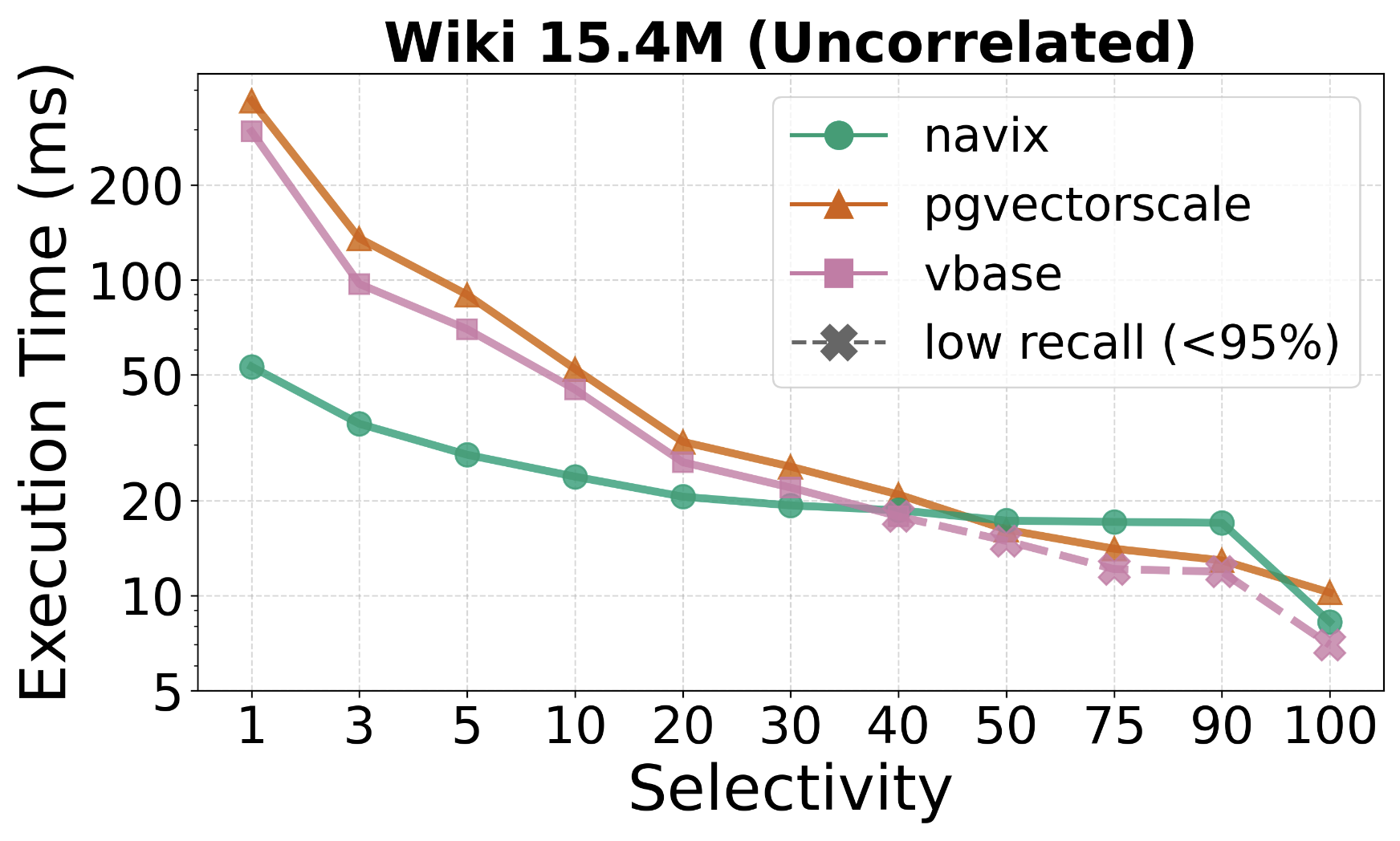
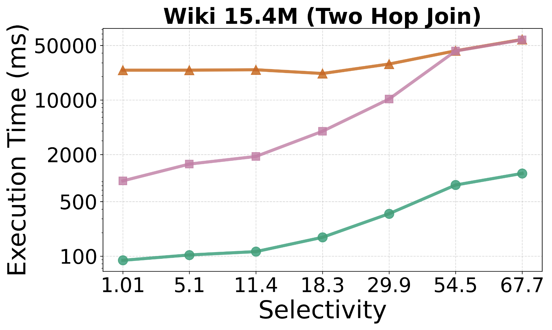
Figure 16. Execution Time vs Selectivity for postfiltering baselines with >95% recall and within 1% of each other

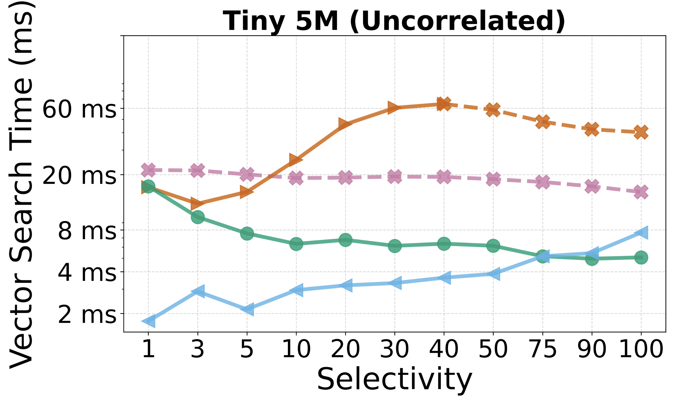
Figure 17. ACORN and iRangeGraph benchmarks at 95% recall.

5.6. iRangeGraph

In our next set of experiments, we compare NaviX against iRangeGraph. iRangeGraph is a specialized vector implementation that supports a limited set of selectivity queries. As such, iRangeGraph is not predicate-agnostic but can be more optimized than NaviX on the range filtering. Specifically, iRangeGraph constructs segmented proximity graphs as sub-indices for different ranges and merges them during search time to support arbitrary ranges.

Since iRangeGraph is implemented using the in-memory HNSWLib (Meta, 2018b), we used FAISS-Navix as a comparison point. Since iRangeGraph supports range selection sub-queries and our uncorrelated workloads are based on range filters, we repeated our experiments on uncorrelated workloads. iRangeGraph only supports L2 distance, so we used GIST and Tiny workloads, which use L2 metric. For reference, Table 6 shows the indexing time of iRangeGraph on these datasets, which is 13.3x and 10.8x slower than FAISS-Navix. Part of this is also due to the fact iRangeGraph creates a larger index. Specifically, on GIST, the size of the iRangeGraph index is 1.2 GB, while FAISS-Navix’s size is 0.3 GB excluding the size of actual vectors. On Tiny, the index sizes of iRangeGraph and FAISS-Navix are, respectively, 6.8 GB and 1.3 GB.

Figure 17 shows our results. Overall, iRangeGraph is more performant than Faiss-Navix at low selectivity levels. This is expected since iRangeGraph efficiently prunes sub-indices to search only those with overlapping ranges, which reduces the number of smaller sub-indices that need to be searched as selectivity decreases. Therefore, unlike all baselines, whose performance degrades as selectivities decrease, iRangeGraph’s performance gets better. FAISS-Navix’s performance becomes more competitive as selectivities increase and at very high selectivity levels, as expected, iRangeGraph loses its performance advantage over FAISS-Navix.

5.7. PGVectorScale and VBase

In this section, we compare NaviX against postfiltering-based systems. We begin by studying the behavior of these systems in Wiki uncorrelated workload. Our results are shown in Figure 16. Our observation for this experiment is similar on the Arxiv workload (see Appendix A.2). However, for Tiny and GIST, both postfiltering systems were unable to reach 95% target recall. PGVectorScale achieves 39.65% and 39.39%, whereas VBase achieves 74.09% and 81.26% for Tiny and GIST workloads respectively. Therefore, we omit these experiments. We can break the cost of postfiltering approaches into three main components:

• Preprocessing cost, if any, to prepare any intermediate tables that are needed to check if a streamed vector is in $S$ or not.

• Vector search cost of streaming nearest neighbors from closest to furthest to $k$. This is determined by the likelihood of vectors in the nearest neighbors of $v_{Q}$ being in $S$. The major factor that determines this is the selectivity level.

• Verification cost of checking if a streamed vector is in $S$ or not.

In our uncorrelated workloads, observe that at high-selectivity levels, postfiltering approaches have an advantage over prefiltering appraoches. This is the ideal case for postfiltering: there is no preprocessing cost and the verification cost is cheap, a lookup to run a simple predicate on the object ID of the vector tuple. At these selectivity levels, prefiltering approaches, specifically NaviX  pays the upfront cost of running the predicate on all vectors. Therefore postfiltering systems outperform NaviX above 50% selectivity.

As the selectivity decreases, vector search cost increases, as more tuples need to be streamed, so cumulative verification cost also increases. Therefore the performance of postfiltering systems degrades significantly. For example, PGVectorScale’s latency numbers degrade from about 10.22 ms to 334.42 ms. A similar degradation also appears in prefiltering approach, e.g., NaviX  but to a lesser extent because vector search is aware of filtering which helps it to only consider selected nodes to converge faster. Thus, NaviX latency only degrades from 8.26 ms to 53.14 ms.

We next used our correlated workloads. Our results are shown in Figure 16. Although our correlated queries have joins of Person and Chunks, PGVectorScale and VBase plan still do not perform any preprocessing. Their plans stream a Chunk tuple v(cID) from a vector search operator. Then an IndexNestedLoopJoin (INLJ) operator joins $v$ with PersonChunk on cID. If a tuple pc(pID,cID) is found, a predicate on the pID is executed. The primary difference is that now there is a more expensive verification cost. However, the general patterns exist. As expected, queries are broadly easier on positively correlated scenarios than negatively correlated scenarios for all systems, i.e., latencies generally go down. For example, PGVectorScale’s runtimes in the 1% to 22.9% range are 331.38 ms to 2052.44 ms and 28.67 ms to 524.54 ms respectively, in the negatively and positively correlated cases. NaviX is more robust to selectivity changes and its latency numbers are between 71.86 ms to 65.7 ms and 38.86 ms to 29.66 ms.

We also extended our experiments with an additional 2-hop join benchmark on Wiki that represents a graph RAG application (Xu et al., 2024a; LangChain, 2024) use case. In this workload selection subqueries are of the following structure:

⬇

1MATCH (p:persons)-[pr:PersonResource]->(r:Resource)

2 (r)-[rc:ResourceChun k]->(c:Chunk)

3WHERE p.birth_date >= {s_date} AND p.birth_date < {e_date}

4PROJECT GRAPH S(c)

5CALL QUERY_HNSW_INDEX(S, HNSWIndex, v_Q, k) RETURN c.cID

To write an equivalent SQL version, we create a temporary table using SQL’s WITH statement. Unlike our previous experiments, PGVectorScale and VBase generate plans that have preprocessing costs. Specifically, they first materialize the 2-hop join in a temporary table Tmp. Then, for each streamed vector $v$, they check if $v$ joins with any tuple in Tmp in a NestedLoopJoin operator. For vector queries, we used our previous queries in the correlated workloads. Our results are shown in Figure 12. First, these queries are harder than prior queries because the selection subquery is harder. Therefore each system’s performance degrades. Also, observe that every system’s curve is now an upward curve. This is because as selectivity levels increase, even though vector search gets faster, the preprocessing cost for both post and prefiltering systems increases. This is because the size of the 2-hop join that needs to be computed increases, which offsets the costs.

5.7.1. Vector Search with Filtering and two-hop traversal

This benchmark evaluates vector search performance with multi-hop joins and date range filtering. Multi-hop joins, in this case, 2-hop traversal are particularly useful in graph RAG applications. This benchmark also helps identify how postfiltering and prefiltering systems behave in complex query scenarios. Again, we will use the date range filtering to reduce the selectivity of this query.

⬇

1-- CYPHER

2MATCH (p:persons)-[r]->(:resources)-[m]->(e:embeddings)

3WHERE p.birth_date >= {start_date} AND p.birth_date < {end_date}

4CALL ANN_SEARCH(e.embedding, {vector}, 100, {efsearch})

5RETURN e.chunk_id;

6

7

8-- SQL

9with t1 as (

10 SELECT r.wiki_id AS r_wiki_id

11 FROM persons AS p

12 JOIN person_resources AS pr ON p.wiki_id = pr.person_wiki_id

13 JOIN resources AS r ON pr.resource_wiki_id = r.wiki_id

14 WHERE p.birth_date >= {start_date} AND p.birth_date < {end_date}

15 GROUP BY r.wiki_id)

16SELECT e.chunk_id

17FROM embeddings as e, t1

18WHERE e.wiki_id = t1.r_wiki_id

19ORDER BY e.embedding <=> ’{vector}’

20LIMIT 100;

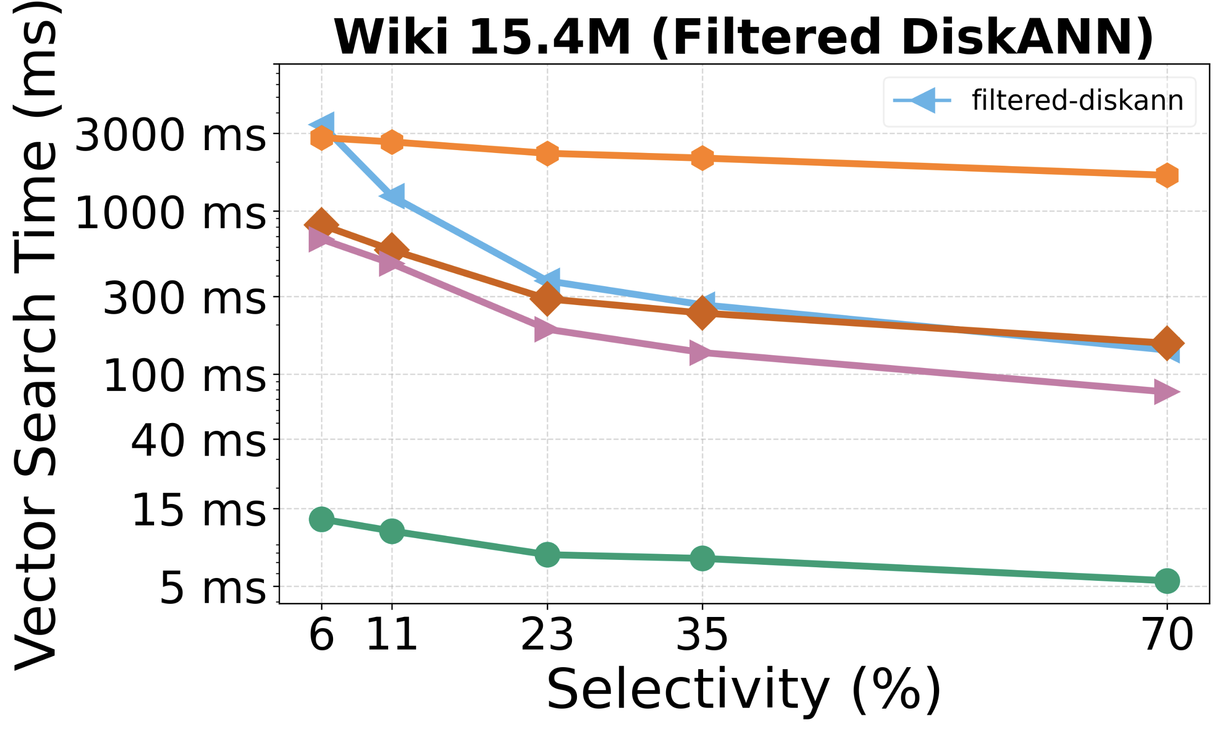
Figure 18. DiskANN and Filtered-DiskANN benchmarks at 95% recall.

5.8. DiskANN and Filtered-DiskANN

5.8.1. DiskANN comparisons

We next compare NaviX with DiskANN (Subramanya et al., 2019) and FilteredDiskANN (Gollapudi et al., 2023), which are two disk-based proximity graph-based vector indices. Our goal is to evaluate the disk-based performance of NaviX. DiskANN is a proximity graph-based index optimized for search on SSDs. It stores each vector and its corresponding adjacency list in a single 4KB page while keeping quantized vectors (Jegou et al., 2011), which are compressed versions of the vectors, in memory. During search, it uses the quantized vectors and performs disk I/O only to read the index graph. After search, it reads the actual vectors and reranks them using actual distances.

Since DiskANN and Navix have very different designs, it is difficult to have very controlled experiments. However, to focus on benchmarking the disk performance of Navix, we ran NaviX in the following configurations:

• NaviX-cold: We start up the system and just measure the first cold run of each query. This forces all accesses to both the vectors and neighborhoods to do disk I/Os.

• NaviX-cold-quant: We quantized the vectors and stored them in an in-memory data structure. We modified our search algorithm to read the quantized vectors from this structure instead of Kuzu’s buffer manager. This gives us a Kuzu configuration that, similar to DiskANN, performs I/Os only to read adjacency lists.

• NaviX-warm-quant-1GB: We give a small amount buffer manager space to NaviX-cold-quant. Before we run each query $q$, we run 1000 random queries, so the adjacency lists are partially cached. We run $q$ only once unlike our previous experiments, because running it multiple times would cache all of the adjacency lists accessed when evaluating $q$ in Kuzu’s buffer manager.

• NaviX-warm-quant-10GB: We give enough buffer manager space to Kuzu to cache most or all of the adjacency lists.

We expect each Kuzu configuration was to outperform the previous one, with performance improvements revealing how different scan operations affect the purely disk-based runtime. We used $R=64$, $LBuild=200$ as DiskANN index configurations. Since Kuzu currently lacks asynchronous I/O support, we set DiskANN’s asynchronous I/O count to 1 as well. Before running each Navix benchmark, we flushed the file system cache.

Since DiskANN does not support filters, we ran experiments on our largest dataset Wiki using the uncorrelated workload queries without filters. Our results are shown in Figure 18. We observe that scanning of vectors is the major contributor to the runtime. This is because the largest performance difference is between NaviX-cold and NaviX-cold-quant. Observe that DiskANN, which only performs disk I/O on scanning adjacency lists outperforms NaviX-cold by a major factor, between 25.07x and 26.72x. However, when we also cache the vectors in memory in quantized way, Kuzu-NaviX-cold-quant closes the performance gap significantly to between 1.79x and 1.92x. DiskANN is still more performant than NaviX-cold-quant, which we attribute to DiskANN’s more optimized I/O path. Specifically, Kuzu requires two random I/Os to read each adjacency list: one to read the metadata i.e. offset and size of its CSRs, and another to read the actual adjacency list. In addition, while DiskANN performs direct I/O, Kuzu always scans through the operating system.

We next observe that even with a small amount of buffer manager cache, Kuzu-NaviX-warm-quant-1GB outperforms DiskANN. This is primarily because we store adjacency lists and vectors separately, thus within a single 4KB page we can pack more adjacency lists and cache more effectively. Finally, by caching more of the index in NaviX-warm-quant-10GB, we can obtain run times that match our previous experiments in Figure 10 (e.g., around 5ms at 95% recall), which are between 13.9x and 10.9x faster than DiskANN (e.g., DiskANN takes 60.27ms at 95% recall). These results highlight one advantage of implementing a vector index natively inside a DBMS. Specifically, since DBMSs already have caching mechanisms, the performance of the vector index automatically improves with additional memory resources in the system.

5.8.2. FilteredDiskANN comparisons

We next compared the performance of the same NaviX configurations against FilteredDiskANN. Briefly, FilteredDiskANN is similar to DiskANN except it supports single-label filtering on a low-cardinality label set (up to 5,000 unique labels). It modifies the proximity graph by creating extra edges between nodes with the same label.

We generated 200 unique random labels and assigned them to each vector in our Wiki dataset with zipf distribution using FilteredDiskANN’s synthetic label generation tool. We fixed the recall rate to 95% as before and used the same index building parameters as in the DiskANN benchmark. FilteredDiskANN can only answer queries that ask for one label, which limits the selectivities we can use. We varied the labels from least selective query, which had a selectivity of 70% to 6%. Our results are shown in Figure 18. Our results are similar to our DiskANN results except even NaviX-cold-quant now outperforms FilteredDiskANN. We attribute this to NaviX’s adaptive-local being a more efficient filtered search algorithm than FilteredDiskANN. The inefficiency of FilteredDiskANN has also been observed in previous work (Patel et al., 2024).

6. Related Work

Our work is related to prior work from several areas:
Approximate Nearest Neighbours Indices: Existing indices that are used for approximate kNN queries can be broadly categorized into two: (i) clustering-based indices (Guo et al., 2020; Sun et al., 2023; Chen et al., 2021; Jegou et al., 2011; Gionis et al., 1999); and (ii) graph-based indices (Fu et al., 2019; Subramanya et al., 2019; Ono and Matsui, 2023; Malkov and Yashunin, 2020). NaviX adopts HNSW, which is a graph-based index. Broadly, clustering based indices partitions the n-dimensional space into different partitions around a set of centroid vectors. Then given a query vector $v_{Q}$, one or more of these partitions are searched to find kNNs of $v_{Q}$. IVF (Jegou et al., 2011; Meta, 2018a) is one of the most used clustering-based approaches. Locality sensitive hashing (Gionis et al., 1999) is another approach to cluster the data based on hashing. In contrast, graph-based indices form a proximity graph across vectors. RNN-Descent (Ono and Matsui, 2023), Vamana (Subramanya et al., 2019), and HNSW (Malkov and Yashunin, 2020) are graph-based indices which rely on proximity graphs, where vectors that are close to each other are connected with each other to form a graph. Graph-based indices are empirically shown to be superior in terms of recall and performance compared to clustering-based approaches (Aumüller et al., 2020).

Predicate-agnostic Vector Search: Several prior DBMSs, vector databases, or vector search systems are capable of evaluating predicate-agnostic vector search queries. These systems adopt pre- or postfiltering or a mix of these approaches. They also adopt graph or clustering-based indices, or a mix of these. We covered Weaviate, Milvus, PGVectorScale, and VBase in prior sections. We cover Acorn and AnalyticDB-V here.

AnalyticDB-V (Wei et al., 2020) is a distributed analytical RDBMS that implements a mix of HNSW index and a compressed clustering-based index called Voronoi Graph Product Quantization (VGPQ) index. The primary index is VGPQ. The newly inserted vectors are first inserted into an HNSW index and periodically merged into the VGPQ index. Since the primary index is VGPQ, the HNSW search is not the bottleneck in predicate-agnostic search queries. On the VGPQ index, AnalyticDB-V performs a mix of post- and prefiltering approach based on the estimated selectivity of the selection subquery.

Specialized indices for predicates on low cardinality attributes: Several prior works have developed graph-based indices that can evaluate predicate-aware vector search queries. These approaches assume a set of predicates, or the structures of these predicates, are known apriori and construct indices whose edges contain extra edges that can be used to evaluate these predicates. We covered Filtered-DiskANN (Gollapudi et al., 2023) in Section 5.8. NHQ (Cai et al., 2024) and HQANN (Wu et al., 2022) are approaches that encode the attribute to filter on directly into the vector as a new dimension and use this during index construction to create extra edges between similar attribute vectors. This method works on small cardinality attributes and on simple filtering operations. HQI(Mohoney et al., 2023) partitions the index based on attributes whose cardinality can be at most 20. This allows searching within a one or a set of partitions to evaluate equality or range queries on this attribute domain.

Finally, SeRF(Zuo et al., 2024) and iRangeGraph(Xu et al., 2024b), which we also compared against in Section 5.6, support arbitrary range filtering queries on an attribute in the context of graph-based vector indices. At a high level, both approaches construct segmented sub-indices for different ranges and merge them together to support arbitrary ranges. However, since these approaches require constructing many sub-indices, they are significantly slower during index construction.

Overall, these specialized indices are generally highly limited in terms of the predicates or the structures of their selection subqueries. For example, they are not designed to support selection subqueries that includes join or filters on string-based predicates.

Native Vector Indices in DBMS: We compared NaviX against PGVectorScale and VBase in Section 5.7. Several other DBMSs or DBMS extensions also support vector indices. PGVector (Kane, [n.d.]) and PASE (Yang et al., 2020) are vector index extension of PostgresSQL. Finally DuckDB and Neo4j also support vector indices. DuckDB uses the USearch (Vardanian, [n.d.]b) library and Neo4j uses Apache Lucene (Cutting, [n.d.]). Unlike our approach, which integrates a native vector index, these systems use separate indices and do not support predicate agnostic search.

7. Conclusions

We presented the design and implementation of NaviX, a native vector index designed for GDBMSs that can evaluate predicate agnostic vector search queries. NaviX leverages some of the core capabilities of the underlying GDBMS, such as its disk-based adjacency list storage and querying capabilities to compute selected vectors in filtered vector search queries. We also introduced an optimization to perform distance computation more efficiently inside a DBMS. Our optimization runs the distance computations directly inside the DBMS’s buffer manager cache. For filtered vector search, NaviX adopts the prefiltering approach and uses a novel search heuristic called adaptive-local, which utilizes the selectivity information in the selected subset $S$ to decide through simple rules which exploration heuristic to pick per candidate vector. To capture possible correlations of $S$ with a query vector $v_{Q}$, adaptive-local uses the local selectivity of the neighbors of each candidate vector it explores during search. Our results show that NaviX is efficient and robust and is competitive with or outperforms both existing prefiltering and postfiltering based systems and heuristics under a variety of query workloads with different selectivities and correlations.

Appendix A Appendix

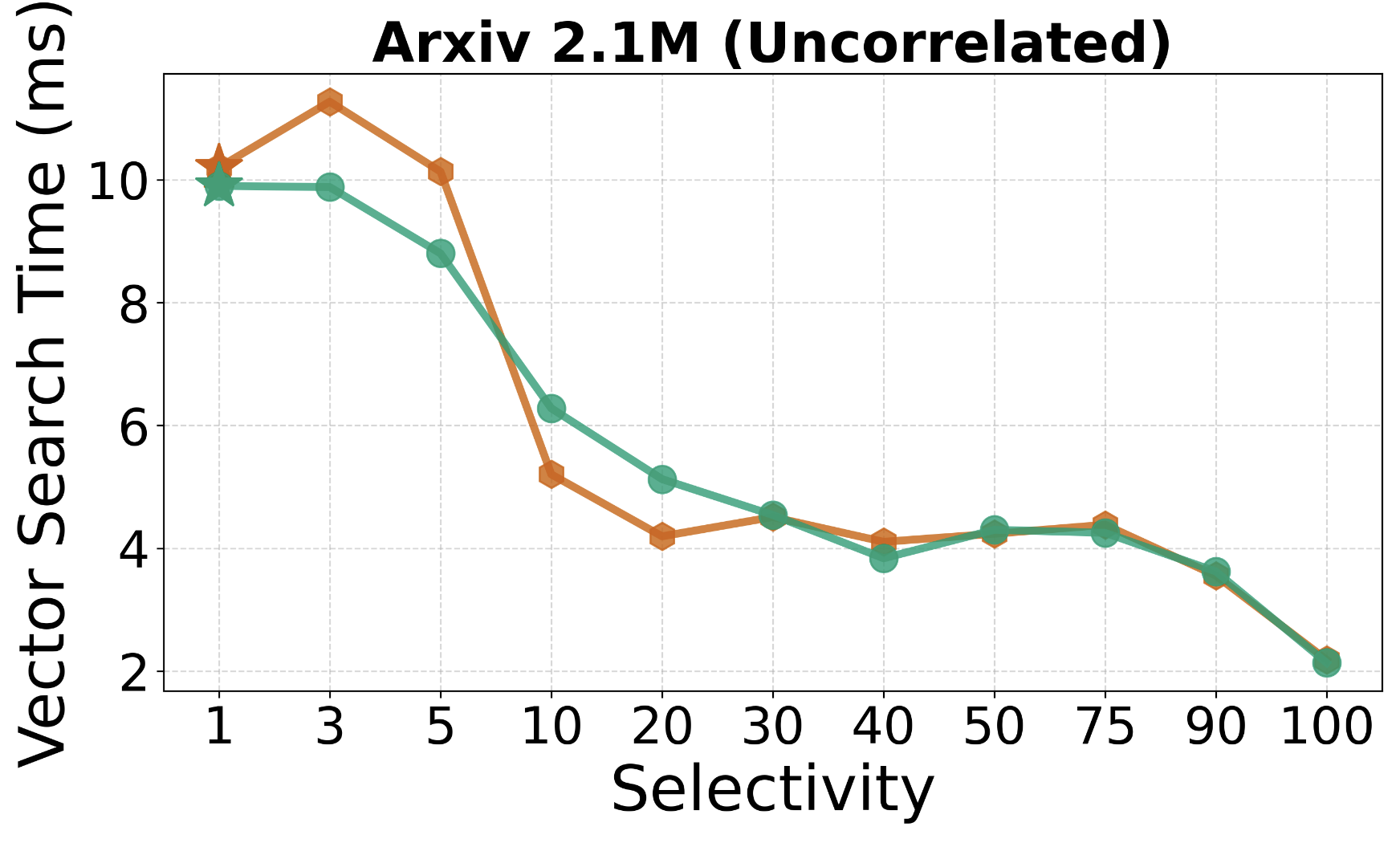
Figure 19. Vector search time vs selectivity for NaviX and adaptive-g within 95% to 95.5% recall

A.1. Evaluation of Adaptive-G and Navix For Other Uncorrelated Workloads:

As mentioned in Section 5.3, we present vector search time for NaviX and adaptive-g for other uncorrelated workloads i.e. Tiny, GIST, and Arxiv. Figure 19 demonstrates vector search time across different selectivities. NaviX and adaptive-g perform similarly to each other except at lower selectivities for Tiny and GIST, where NaviX outperforms adaptive-g by up to 30%. This performance advantage occurs because NaviX can make better decisions when switching between different heuristics based on the local selectivity of the index traversal region.

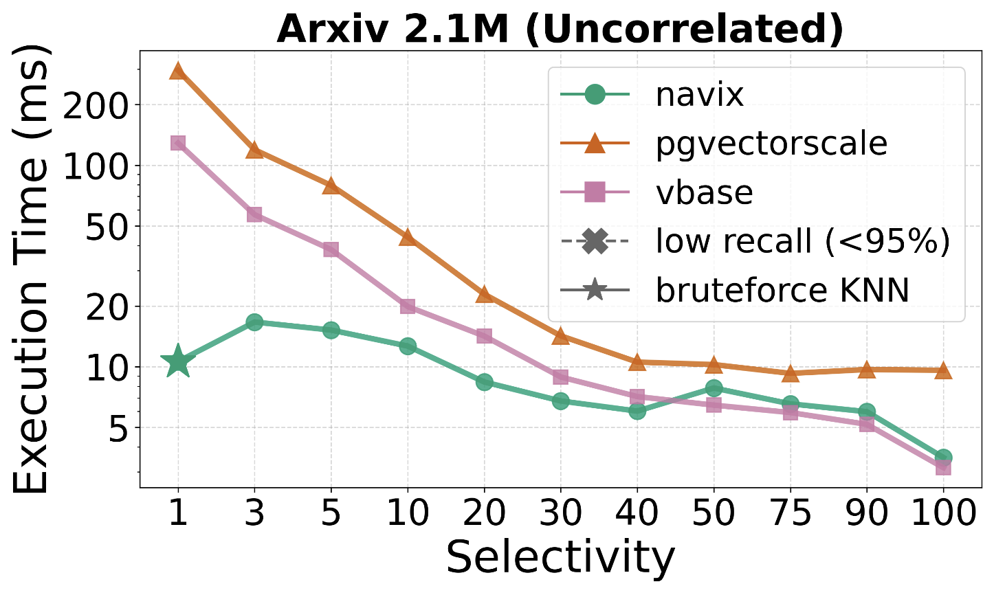
Figure 20. Execution Time vs Selectivity for postfiltering baselines with >95% recall and within 1% of each other

A.2. Evaluation of Postfiltering Baselines for Arxiv Uncorrelated Workload:

We extend the experiments in Section 5.7 with the Arxiv uncorrelated workload in Figure 20. The results are similar to the Wiki uncorrelated workload in Section 5.7: both postfiltering systems degrade significantly in mid to lower selectivities where NaviX outperforms both of them. For higher selectivities, the difference is not as significant. However, NaviX slightly outperforms PGVectorScale since the Arxiv dataset is smaller, thus the majority of the cost is due to vector search time rather than prefiltering time.

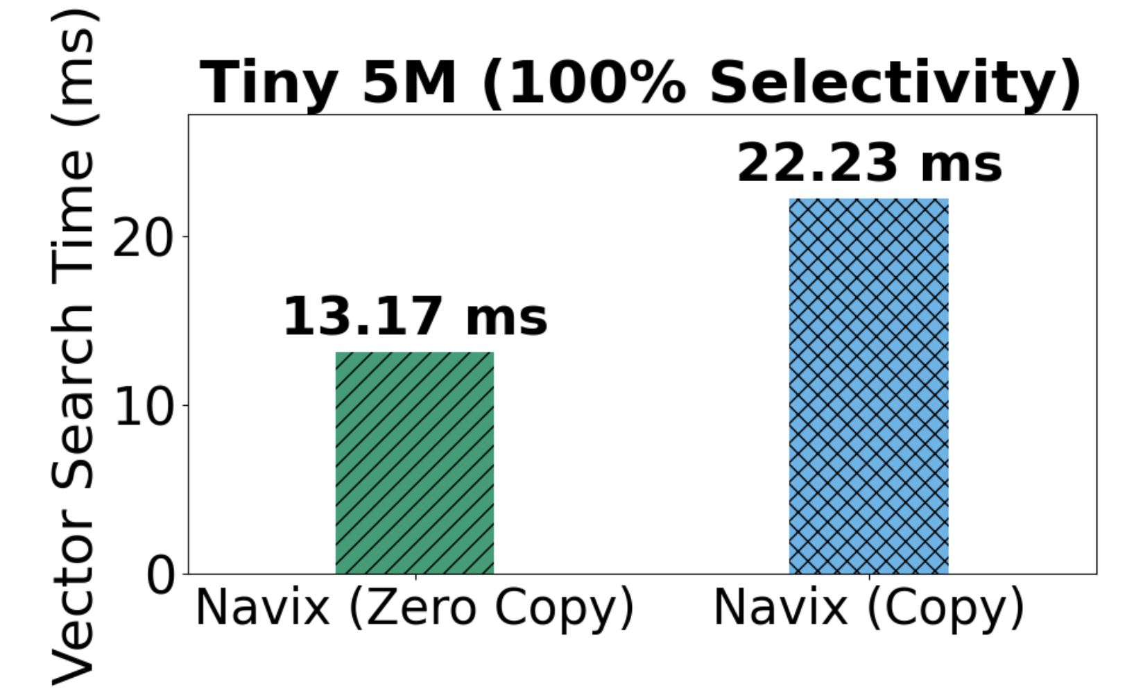
Figure 21. Vector Search Time with and without zero-copy optimization for 95% recall

A.3. Evaluation of In-BM Distance Calculations:

In this evaluation, we do an ablation study on how much performance benefits our in-bm distance calculation optimization provides. As shown in Figure 21, we used the Tiny dataset at 100% selectivity. We turned the in-bm distance calculation optimization off in NaviXẆe refer to this configuration as NaviX-copy. Figure 21 shows our results. We see that the in-bm optimization improves the performance of NaviX by 1.6x, demonstrating its importance for DBMSs that use a BM to scan their vectors into their vector search operators.

Figure 22. Vector Search Time vs Selectivity for ACORN and Faiss-Navix baselines at different recalls

A.4. Comparison Against ACORN at Different Recalls

As mentioned in Section 5.5, Figure 22 present remaining results comparing Faiss-NaviX and Acorn at 90% and 97% recall levels on our workloads. The findings align with our previous results where Faiss-NaviX consistently outperforms both Acorn configurations i.e. Acorn-1 and Acorn-10.

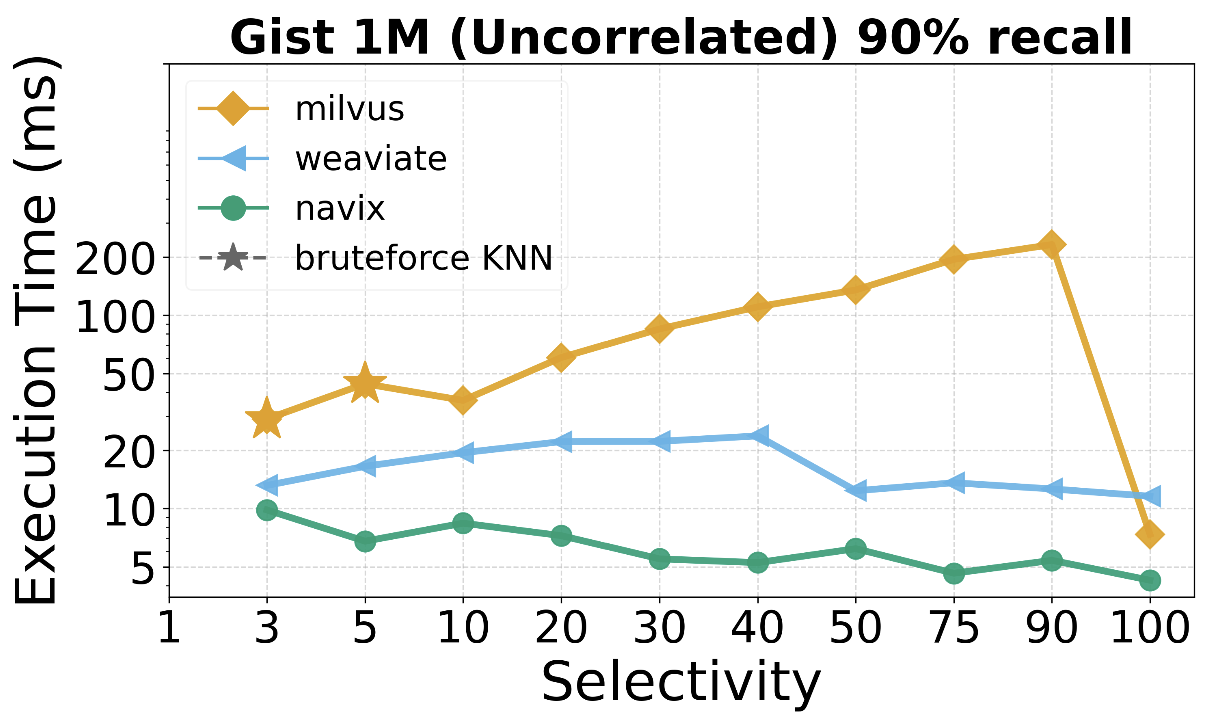
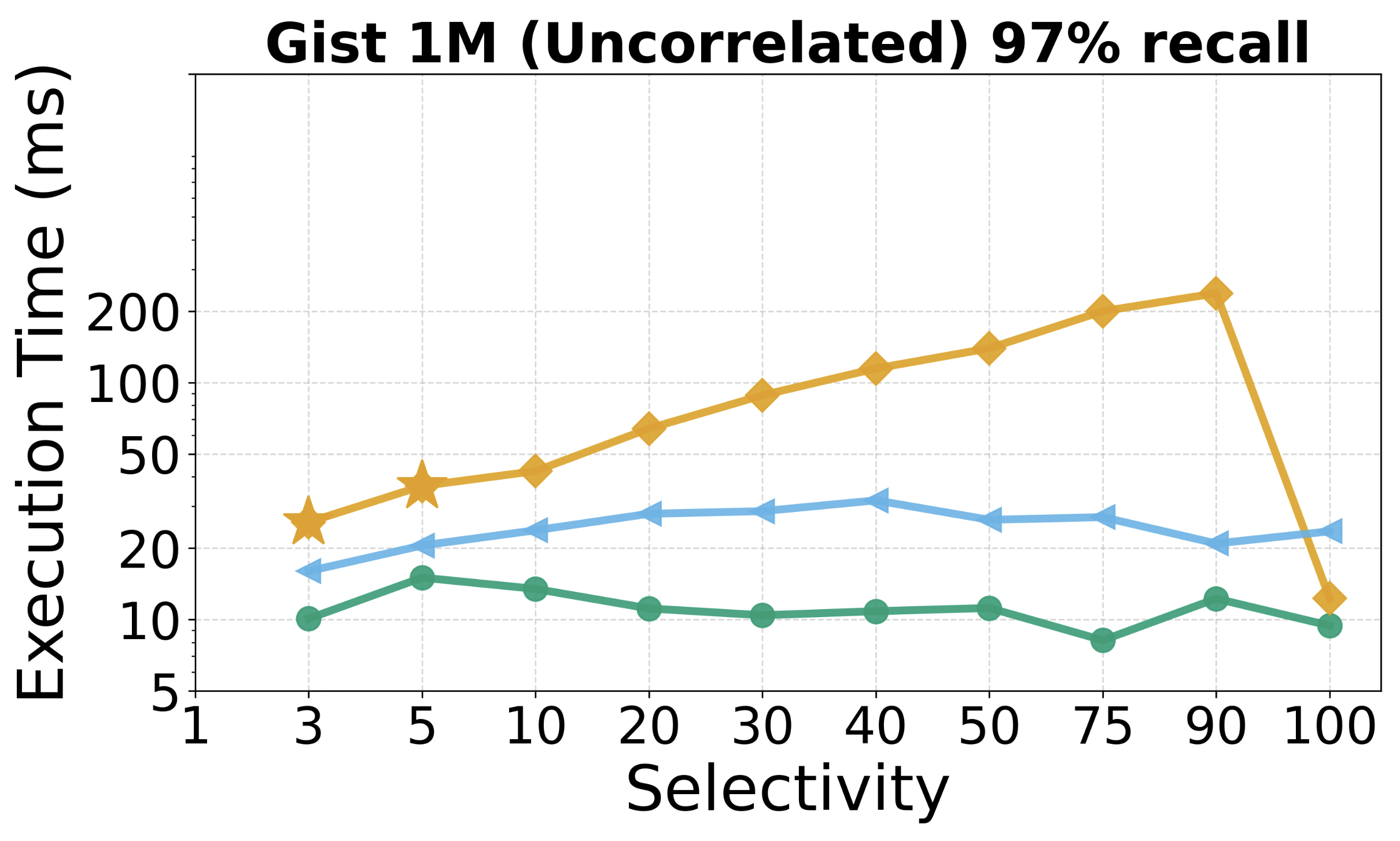
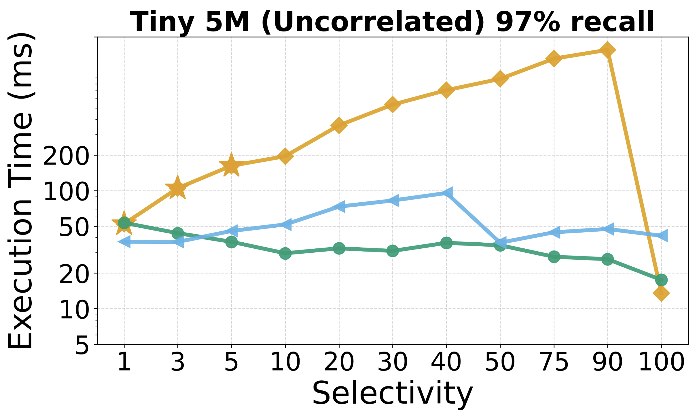
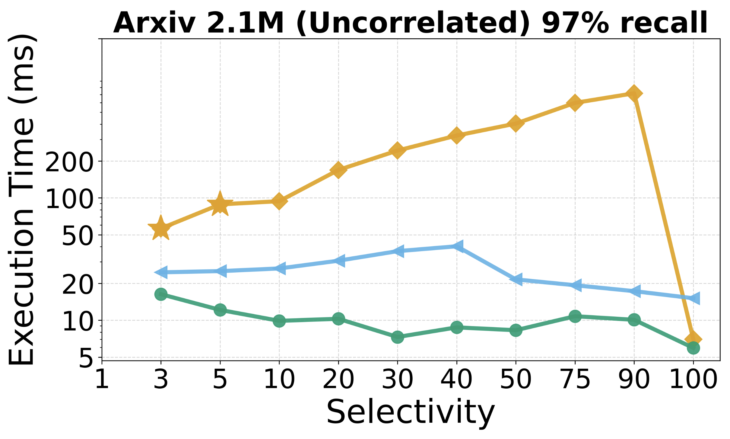
Figure 23. Execution Time vs Selectivity for Weaviate and Milvus baselines at different Recalls

A.5. Comparison Against Weaviate and Milvus at Different Recalls

As mentioned in Section 5.4, Figure 23 present remaining results comparing NaviX with Weaviate and Milvus at 90% and 97% recall levels on our workloads. The findings align with our previous results where NaviX is competitive or outperforms both Weaviate and Milvus at different selectivities.

References

- (1)
- kuz (2024) 2024. Kuzu Github Repo. https://github.com/kuzudb/kuzu.
- Abadi et al. (2012) Daniel Abadi, Peter Boncz, Stavros Harizopoulos, Stratos Idreos, and Samuel Madden. 2012. The Design and Implementation of Modern Column-Oriented Database Systems. Foundations and Trends® in Databases 5, 3 (2012).
- arXiv ([n.d.]) arXiv. [n.d.]. Arxiv Dataset. https://info.arxiv.org/help/bulk_data/index.html.
- Aumüller et al. (2020) Martin Aumüller, Erik Bernhardsson, and Alexander Faithfull. 2020. ANN-Benchmarks: A benchmarking tool for approximate nearest neighbor algorithms. Inf. Syst. 87, C (2020).
- Cai et al. (2024) Yuzheng Cai, Jiayang Shi, Yizhuo Chen, and Weiguo Zheng. 2024. Navigating Labels and Vectors: A Unified Approach to Filtered Approximate Nearest Neighbor Search. SIGMOD 2, 6 (2024).
- Canada ([n.d.]) Compute Canada. [n.d.]. Compute Canada Cedar. https://docs.alliancecan.ca/wiki/Cedar.
- Chen et al. (2021) Qi Chen, Bing Zhao, Haidong Wang, Mingqin Li, Chuanjie Liu, Zengzhong Li, Mao Yang, and Jingdong Wang. 2021. SPANN: highly-efficient billion-scale approximate nearest neighbor search. In NeurIPS.
- Cutting ([n.d.]) Doug Cutting. [n.d.]. Apache Lucene. https://lucene.apache.org/.
- DBpedia (2024) DBpedia. 2024. DBpedia Latest Dataset. https://databus.dbpedia.org/dbpedia/collections/latest-core.
- Feng et al. (2023) Xiyang Feng, Guodong Jin, Ziyi Chen, Chang Liu, and Semih Salihoğlu. 2023. Kùzu Graph Database Management System. In CIDR.
- Fu et al. (2019) Cong Fu, Chao Xiang, Changxu Wang, and Deng Cai. 2019. Fast approximate nearest neighbor search with the navigating spreading-out graph. PVLDB 12, 5 (2019).
- Gionis et al. (1999) Aristides Gionis, Piotr Indyk, and Rajeev Motwani. 1999. Similarity Search in High Dimensions via Hashing. In VLDB.
- Gollapudi et al. (2023) Siddharth Gollapudi, Neel Karia, Varun Sivashankar, Ravishankar Krishnaswamy, Nikit Begwani, Swapnil Raz, Yiyong Lin, Yin Zhang, Neelam Mahapatro, Premkumar Srinivasan, Amit Singh, and Harsha Vardhan Simhadri. 2023. Filtered-DiskANN: Graph Algorithms for Approximate Nearest Neighbor Search with Filters. In ACM Web Conference.
- Guo et al. (2020) Ruiqi Guo, Philip Sun, Erik Lindgren, Quan Geng, David Simcha, Felix Chern, and Sanjiv Kumar. 2020. Accelerating large-scale inference with anisotropic vector quantization. In ICML.
- Gupta et al. (2021) Pranjal Gupta, Amine Mhedhbi, and Semih Salihoglu. 2021. Columnar Storage and List-based Processing for Graph Database Management Systems. PVLDB 14, 11 (2021).
- HuggingFace ([n.d.]) HuggingFace. [n.d.]. MTEB Embedding Leaderboard. https://huggingface.co/spaces/mteb/leaderboard.
- Jegou et al. (2008) Herve Jegou, Matthijs Douze, and Cordelia Schmid. 2008. Hamming Embedding and Weak Geometric Consistency for Large Scale Image Search. In ECCV.
- Jegou et al. (2011) Herve Jegou, Matthijs Douze, and Cordelia Schmid. 2011. Product Quantization for Nearest Neighbor Search. IEEE PAMI 33, 1 (2011).
- Kane ([n.d.]) Andrew Kane. [n.d.]. PGVector. https://github.com/pgvector/pgvector.
- LangChain (2024) LangChain. 2024. Enhancing RAG-based application accuracy by constructing and leveraging knowledge graphs. https://blog.langchain.dev/enhancing-rag-based-applications-accuracy-by-constructing-and-leveraging-knowledge-graphs/.
- Lewis et al. (2020) Patrick Lewis, Ethan Perez, Aleksandra Piktus, Fabio Petroni, Vladimir Karpukhin, Naman Goyal, Heinrich Küttler, Mike Lewis, Wen-tau Yih, Tim Rocktäschel, Sebastian Riedel, and Douwe Kiela. 2020. Retrieval-augmented generation for knowledge-intensive NLP tasks. In NeurIPS.
- Li et al. (2018) Jinfeng Li, Xiao Yan, Jian Zhang, An Xu, James Cheng, Jie Liu, Kelvin K. W. Ng, and Ti-chung Cheng. 2018. A General and Efficient Querying Method for Learning to Hash. In SIGMOD.
- Malkov and Yashunin (2020) Yu A. Malkov and D. A. Yashunin. 2020. Efficient and Robust Approximate Nearest Neighbor Search Using Hierarchical Navigable Small World Graphs. IEEE PAMI 42, 4 (2020).
- Meta (2018a) Meta. 2018a. Faiss. https://github.com/facebookresearch/faiss.
- Meta (2018b) Meta. 2018b. HNSWLib. https://github.com/nmslib/hnswlib.
- Milvus (2024) Milvus. 2024. Milvus v2.5.0. https://milvus.io/.
- Mohoney et al. (2023) Jason Mohoney, Anil Pacaci, Shihabur Rahman Chowdhury, Ali Mousavi, Ihab F. Ilyas, Umar Farooq Minhas, Jeffrey Pound, and Theodoros Rekatsinas. 2023. High-Throughput Vector Similarity Search in Knowledge Graphs. SIGMOD 1, 2 (2023).
- Navarro (2002) Gonzalo Navarro. 2002. Searching in metric spaces by spatial approximation. VLDB 11, 1 (2002).
- Oliva and Torralba (2001) Aude Oliva and Antonio Torralba. 2001. Modeling the Shape of the Scene: A Holistic Representation of the Spatial Envelope. Int. J. Comput. Vision 42, 3 (2001).
- Ono and Matsui (2023) Naoki Ono and Yusuke Matsui. 2023. Relative NN-Descent: A Fast Index Construction for Graph-Based Approximate Nearest Neighbor Search. In ACM MM.
- OpenAI ([n.d.]) OpenAI. [n.d.]. OpenAI O1 Large Language Model. https://openai.com/o1/.
- Parquet ([n.d.]) Apache Parquet. [n.d.]. Parquet Documentation. https://parquet.apache.org/docs/.
- Patel et al. (2024) Liana Patel, Peter Kraft, Carlos Guestrin, and Matei Zaharia. 2024. ACORN: Performant and Predicate-Agnostic Search Over Vector Embeddings and Structured Data. In SIGMOD.
- Poliakov and Shvai (2024) Mykhailo Poliakov and Nadiya Shvai. 2024. Multi-Meta-RAG: Improving RAG for Multi-Hop Queries using Database Filtering with LLM-Extracted Metadata. arXiv:arXiv:2406.13213 https://arxiv.org/abs/2406.13213
- Qdrant ([n.d.]) Qdrant. [n.d.]. ANN Filtered Dataset. https://github.com/qdrant/ann-filtering-benchmark-datasets.
- Sarmah et al. (2024) Bhaskarjit Sarmah, Dhagash Mehta, Benika Hall, Rohan Rao, Sunil Patel, and Stefano Pasquali. 2024. HybridRAG: Integrating Knowledge Graphs and Vector Retrieval Augmented Generation for Efficient Information Extraction. In ICAIF. Association for Computing Machinery, New York, NY, USA. https://doi.org/10.1145/3677052.3698671
- Search (2024) Nova Search. 2024. stella_en_400M_v5 Embedding Model. https://huggingface.co/NovaSearch/stella_en_400M_v5.
- Sehgal and Salihoğlu ([n.d.]) Gaurav Sehgal and Semih Salihoğlu. [n.d.]. Kuzu Navix Repo. https://github.com/gaurav8297/kuzu.
- Subramanya et al. (2019) Suhas Jayaram Subramanya, Devvrit, Rohan Kadekodi, Ravishankar Krishaswamy, and Harsha Vardhan Simhadri. 2019. DiskANN: fast accurate billion-point nearest neighbor search on a single node. In NeurIPS.
- Sun et al. (2023) Philip Sun, David Simcha, Dave Dopson, Ruiqi Guo, and Sanjiv Kumar. 2023. SOAR: improved indexing for approximate nearest neighbor search. In NeurIPS.
- Timescale (2024) Timescale. 2024. PGVectorScale v0.5.1. https://github.com/timescale/pgvectorscale.
- Torralba et al. (2008) Antonio Torralba, Rob Fergus, and William T. Freeman. 2008. 80 Million Tiny Images: A Large Data Set for Nonparametric Object and Scene Recognition. IEEE PAMI 30, 11 (2008).
- Toussaint (1980) Godfried T. Toussaint. 1980. The Relative Neighbourhood Graph of a Finite Planar Set. Pattern Recognition 12, 4 (1980).
- Transformers ([n.d.]) Sentence Transformers. [n.d.]. all-MiniLM-L6-v2 Embedding Model. https://huggingface.co/sentence-transformers/all-MiniLM-L6-v2.
- Vardanian ([n.d.]a) Ash Vardanian. [n.d.]a. SimSIMD. https://github.com/ashvardanian/SimSIMD.
- Vardanian ([n.d.]b) Ash Vardanian. [n.d.]b. USearch. https://github.com/unum-cloud/usearch.
- Wang et al. (2021) Jianguo Wang, Xiaomeng Yi, Rentong Guo, Hai Jin, Peng Xu, Shengjun Li, Xiangyu Wang, Xiangzhou Guo, Chengming Li, Xiaohai Xu, Kun Yu, Yuxing Yuan, Yinghao Zou, Jiquan Long, Yudong Cai, Zhenxiang Li, Zhifeng Zhang, Yihua Mo, Jun Gu, Ruiyi Jiang, Yi Wei, and Charles Xie. 2021. Milvus: A Purpose-Built Vector Data Management System. In SIGMOD.
- Weaviate ([n.d.]) Weaviate. [n.d.]. Filtered Vector Search | Weaviate - vector database. https://weaviate.io/developers/weaviate/concepts/filtering.
- Weaviate (2024a) Weaviate. 2024a. How we speed up filtered vector search with ACORN. https://weaviate.io/blog/speed-up-filtered-vector-search.
- Weaviate (2024b) Weaviate. 2024b. Weaviate v1.28.2. https://weaviate.io/.
- Wei et al. (2020) Chuangxian Wei, Bin Wu, Sheng Wang, Renjie Lou, Chaoqun Zhan, Feifei Li, and Yuanzhe Cai. 2020. AnalyticDB-V: A hybrid analytical engine towards query fusion for structured and unstructured data. PVLDB 13, 12 (2020).
- WikiMedia (2024) WikiMedia. 2024. WikiMedia enwiki Dump. https://dumps.wikimedia.org/enwiki/latest/enwiki-latest-pages-articles.xml.bz2.
- Wu et al. (2022) Wei Wu, Junlin He, Yu Qiao, Guoheng Fu, Li Liu, and Jin Yu. 2022. HQANN: Efficient and Robust Similarity Search for Hybrid Queries with Structured and Unstructured Constraints. In CIKM.
- Xu et al. (2024b) Yuexuan Xu, Jianyang Gao, Yutong Gou, Cheng Long, and Christian S. Jensen. 2024b. iRangeGraph: Improvising Range-dedicated Graphs for Range-filtering Nearest Neighbor Search. SIGMOD 2, 6 (2024).
- Xu et al. (2024a) Zhentao Xu, Mark Jerome Cruz, Matthew Guevara, Tie Wang, Manasi Deshpande, Xiaofeng Wang, and Zheng Li. 2024a. Retrieval-Augmented Generation with Knowledge Graphs for Customer Service Question Answering. In ACM SIGIR.
- Yang et al. (2020) Wen Yang, Tao Li, Gai Fang, and Hong Wei. 2020. PASE: PostgreSQL Ultra-High-Dimensional Approximate Nearest Neighbor Search Extension. In SIGMOD.
- Zhang et al. (2023) Qianxi Zhang, Shuotao Xu, Qi Chen, Guoxin Sui, Jiadong Xie, Zhizhen Cai, Yaoqi Chen, Yinxuan He, Yuqing Yang, Fan Yang, Mao Yang, and Lidong Zhou. 2023. VBASE: Unifying Online Vector Similarity Search and Relational Queries via Relaxed Monotonicity. In OSDI.
- Zuo et al. (2024) Chaoji Zuo, Miao Qiao, Wenchao Zhou, Feifei Li, and Dong Deng. 2024. SeRF: Segment Graph for Range-Filtering Approximate Nearest Neighbor Search. SIGMOD 2, 1 (2024).