AICO: Feature Significance Tests
for Supervised Learning

Abstract

The opacity of many supervised learning algorithms remains a key challenge, hindering scientific discovery and limiting broader deployment—particularly in high-stakes domains. This paper develops model- and distribution-agnostic significance tests to assess the influence of input features in any regression or classification algorithm. Our method evaluates a feature’s incremental contribution to model performance by masking its values across samples. Under the null hypothesis, the distribution of performance differences across a test set has a non-positive median. We construct a uniformly most powerful, randomized sign test for this median, yielding exact $p$-values for assessing feature significance and confidence intervals with exact coverage for estimating population-level feature importance. The approach requires minimal assumptions, avoids model retraining or auxiliary models, and remains computationally efficient even for large-scale, high-dimensional settings. Experiments on synthetic tasks validate its statistical and computational advantages, and applications to real-world data illustrate its practical utility.

1 Introduction

Supervised learning algorithms have become foundational tools across scientific and industrial domains, enabling breakthroughs and transforming key sectors. However, their opacity poses a major challenge, hindering scientific discovery and limiting adoption in high-stakes domains like finance, public policy and health care, where transparency is crucial.

This paper proposes novel testing methods for addressing the opacity of learning algorithms, focusing on the role of an algorithms’s input variables (features). Specifically, we develop a family of hypothesis tests to assess the significance of features in any supervised learning model, whether for regression or classification. The tests are model- and distribution-agnostic: they only require the ability to query the trained model—no assumptions about the model class, data distribution or model target (e.g. conditional mean, quantile) are needed. The computational efficiency of our tests is unprecedented. The procedure does not require retraining or surrogate models, making it well-suited for analyzing complex, high-dimensional algorithms that are costly to train.

The tests are based on a new approach for evaluating the impact of a feature. We quantify a feature’s incremental contribution to a user-defined score function, which measures a model’s predictive or decision-making performance on a test sample. Specifically, we compute the feature effect as the change in score when the model is given the actual value of the feature versus when the feature is masked with a baseline value. This masking approach, which we call Add-In Covariates (AICO), avoids the variance inflation (excess randomness) introduced by permutation methods and the high cost of retraining-based and surrogate-model-based strategies. The score function and masking baseline can be user-specified to align with specific interpretability goals and downstream model use cases; we discuss a number of choices and the associated tradeoffs.

The feature effect measures the impact of a feature’s variability on model score; it represents the importance of a feature at the level of an individual sample. A null-feature’s effect has a distribution across a collection of test samples whose median is non-positive. We construct a uniformly most powerful, randomized sign test for this median. Randomization at the boundary of the critical region ensures the test’s exactness, i.e., its size (type I error probability) matching the user-specified nominal level (e.g. $5\%$). The test delivers exact, randomized feature $p$-values that have, conditionally on the data, a uniform distribution on an interval which can be reported in practice. It is simple, robust and permits an efficient implementation. It requires minimal assumptions, ensuring its broad validity in practice. These properties allow users to make valid inferences regarding a model’s features without relying on large-sample approximations or parametric assumptions.

The median feature effect being tested is a natural measure of feature importance at the population level. We develop randomized, exact-coverage confidence intervals for the median that, together with the $p$-values, enable principled inference regarding feature influence. The availability of confidence intervals distinguishes the median from widely-used algorithmic measures of feature importance (see Section 1.1 below). Moreover, depending on the selection of the masking baseline, the median can have several useful properties. These include robustness to correlation between features, which is common in practice. Furthermore, for linear regression, the median is proportional to the square of the feature’s regression coefficient, which is the canonical measure of importance in the linear context. Finally, we provide conditions guaranteeing that a feature’s median being 0 is equivalent to it being conditionally independent of the response given the remaining features.

Extensive experiments on synthetic “known truth” tasks demonstrate the statistical and computational performance of our approach in nonlinear regression and classification settings. We compare our tests with the recently developed, model-agnostic and non-asymptotic tests of berrett, tansey2018holdout and Lei2018predictive. We also compare with the model-X knockoff procedures of candes2018panning and deepknockoffs for variable selection with false discovery control. Our test is found to be as statistically powerful as the alternatives, with minimal false discovery, while reducing computational costs by several orders of magnitude. Moreover, we show that our feature importance measure is robust to noise in the data, delivering stable feature importance rankings. This contrasts sharply with widely-used algorithmic feature importance measures including SHAP [lundberg2017unified] which are found to be highly sensitive to noise in the data, leading to unstable feature rankings that make it difficult to draw reliable inferences regarding variable importance. Our findings complement the discussion of the theoretical caveats of algorithmic importance measures in verdinelli-wasserman, kumar and others.

Several comprehensive empirical analyses illustrate our testing and feature importance approach in real-world data settings. In the context of a credit scoring task using large ensembles of gradient boosting machines, our approach identifies and ranks several significant features describing past payment behavior and social factors. Interestingly, we find that gender, marital status, and age of card holders (all of which are protected characteristics under US lending laws) are significant predictors of credit card default, after controlling for past payment behavior. In the context of a mortgage state transition prediction task using a recently proposed set-sequence model based on long-convolution architectures [elliot] and trained on extensive panel data, our test identifies time-varying macro-economic variables such as mortgage rates, as well as features summarizing past state transitions as significant predictors of borrower behavior.

The rest of this introduction discusses the related literature. Section 2 introduces the notion of feature effects while Section 3 develops the testing procedure. Section 4 analyzes the median feature effect as an importance measure dual to the test. Section 5 studies the performance of the test and importance measure in synthetic regression and classification settings. Section 6 deploys the test on two real-world data sets. The proofs of technical results are given in an appendix. A Python package implementing our testing and importance procedures is available at https://github.com/ji-chartsiri/AICO.

1.1 Related literature

There is a large body of work developing algorithmic feature importance measures; see burkart-huber for an overview. Popular examples include measures based on Shapley values (e.g. SHAP, see lundberg2017unified and many others), measures based on local approximations (e.g. LIME, see ribeiro2016should), and measures obtained by permutation methods (e.g. breiman, fisher-rudin). These measures provide valuable insight into the role of features but unlike the feature importance measures delivered by our hypothesis testing approach, they typically do not offer statistical guarantees or $p$-values. We demonstrate that algorithmic measures can be highly susceptible to noise in the data so the lack of confidence intervals is concerning. Moreover, algorithmic measures such as SHAP can be biased in the presence of feature correlation [verdinelli-wasserman]. Our approach can deliver importance measures that are robust to feature correlation. Finally, we demonstrate that our method achieves orders-of-magnitude improvements in computational efficiency over widely used algorithmic importance approaches, such as SHAP and permutation scores.

The statistical and econometric literature has developed significance tests for the variables in nonparametric regression models. fan-li, lavergne2000nonparametric, ait-sahalia-bickel, delgado-manteiga, lavergne2015 and others employ kernel methods to construct asymptotic-based testing procedures. white2001statistical, horel-giesecke and fallahgoul and others construct gradient-based asymptotic tests using neural networks. Unlike these tests, ours are model-agnostic, non-asymptotic, deliver exact $p$-values and confidence intervals, and can accommodate a wide range of data structures.

Pursuing a model-agnostic approach, candes2018panning, berrett, tansey2018holdout, janson, bellot, wright and others develop non-asymptotic tests for a conditional independence hypothesis of feature significance in the model-X knockoff setting of candes2018panning. We show that, for an appropriate choice of the masking baseline, our null is generally weaker than the conditional independence null studied in these papers; equivalence holds under additional conditions. Lei2018predictive construct non-asymptotic tests based on the drop in model predictive accuracy due to removing features (LOCO: Leave-out-covariates). We, in contrast, test the improvement in model score due to masking a feature.

The computational requirements of the aforementioned model-agnostic testing procedures are a limiting factor. The LOCO test requires re-training the model for each feature to be tested, which can be prohibitive for feature-rich models that are costly to train. The model-X knockoff procedures require constructing an auxiliary model of the joint feature distribution, which can be as challenging and computationally costly as constructing the model to be tested. In fact, bates show that no algorithm can efficiently compute nontrivial knockoffs for arbitrary feature distributions. Our approach does not require any model re-training or the construction of auxiliary models, delivering an unprecedented degree of computational efficiency. Our numerical results demonstrate that the drastic gains in computational performance we achieve do not come at the expense of statistical performance.

2 Feature effect

We consider i.i.d. data $Z_{1},\ldots,Z_{m}$ with $Z_{i}=(X_{i},Y_{i})$. Here, $X_{i}=(X^{1}_{i},\ldots,X^{d}_{i})$ is a $d$-dimensional feature vector taking values in a set $\mathcal{X}$ and $Y_{i}$ is a response taking values in a set $\mathcal{Y}$. In a typical regression setting with tabular data, $\mathcal{X}\subseteq\mathbb{R}^{d}$ and $\mathcal{Y}=\mathbb{R}$. We make no assumptions on the population law $\mathbb{P}$ from which $Z_{i}$ is sampled.

We take as given a random split of $[m]=\{1,\ldots,m\}$ into non-intersecting subsets $I_{1}$ and $I_{2}$, which are used for training/validation and testing purposes, respectively. This partitioning is standard in supervised learning settings. In our testing framework, data splitting facilitates post-selection inference.

We also take as given a model (algorithm) $f:\mathcal{X}\to\mathcal{M}$ trained on $\{Z_{i}\}_{i\in I_{1}}$, which is to be tested. We do not make any assumptions on the form of the modeling target; $f$ could represent $\mathbb{E}(Y_{i}|X_{i})$, a conditional quantile, or some other statistic of $Y_{i}$. We also do not impose assumptions on the training criterion (eg. $L_{2}$ error) or approach (eg. empirical risk minimization) being used for training.

We would like to test the statistical significance of a feature $\ell\in[d]$ under the model $f$. (Unless noted otherwise, $\ell$ is fixed.) In the special case that $f$ is linear, standard asymptotic procedures such as the $t$-test are available. We develop a simple, non-asymptotic and model-agnostic testing procedure that does not require a special model structure, and is valid much more broadly for models $f$ of essentially any form.

We consider the impact on model performance of a feature’s variability across the test set $I_{2}$. Performance is measured by a deterministic score function $S:\mathcal{M}\times\mathcal{Y}\to\mathbb{R}$, which relates model output to response. Specifically, for a given feature value $x\in\mathcal{X}$ and response value $y\in\mathcal{Y}$, the score $S(f(x),y)$ evaluates the quality of the model output $f(x)$ in view of $y$. Higher scores reflect better performance. A natural choice for $S$ is the negative of the loss function used for the training of $f$. Examples include the negative $L_{2}$ loss $S(m,y)=-(m-y)^{2}$ in a regression context, the negative pinball loss in a quantile regression context, or the negative (binary or multi-class) cross-entropy loss in a classification context. With these specifications $S$ measures predictive accuracy. Other specifications of $S$ can measure model performance (e.g. revenue) in the context of a downstream screening or decisioning application of $f$, for example the financial loss caused by a poor decision due to mis-classification. Finally, we can specify a function $S$ that does not depend on the second argument representing the response, to measure the behavior (e.g. sensitivity) of the model output on its own, without reference to the response.

We evaluate the effect on model score of a feature’s variability across the test set. For each $i\in I_{2}$ we construct from $X_{i}$ a baseline feature value $\underline{X}_{i}\in\mathcal{X}$ serving as a reference and a comparison feature value $\overline{X}_{i}\in\mathcal{X}$. In the baseline, the value of the feature to be tested is masked with a reference value whose choice is further discussed below. The comparison value $\overline{X}_{i}$ is unmasked so that the predicted response $f(\overline{X}_{i})$ can harness the actual sample $i$ value of the feature to be tested. We propose to measure the feature effect by the resulting score improvement.

Definition 2.1 (Feature Effect).

For a given score function $S$, baseline feature value $\underline{X}_{i}$ and comparison feature value $\overline{X}_{i}$, the feature effect on test sample $i\in I_{2}$ is the score delta

$$\Delta_{i}=S(f(\overline{X}_{i}),Y_{i})-S(f(\underline{X}_{i}),Y_{i}).$$

Note that masking feature values for purposes of measuring a feature effect has significant advantages over alternative approaches such as randomly shuffling feature values (e.g. breiman and fisher-rudin) or dropping a feature from the feature vector. Shuffling introduces excess variance into the measurement procedure and dropping features requires training sub-models, which (drastically) reduces the computational efficiency of the measurement procedure. Our masking approach avoids these issues.

2.1 Baseline and comparison features

Along with the selection of the score function $S$, the selection of baseline and comparison feature values enables users to tailor the feature effect to the model and data structures at hand as well as the testing objectives. We provide a conceptional framework and several examples. Throughout, fix a feature $\ell\in[d]$ that is to be tested; our notation usually suppresses the dependence on $\ell$. We start by selecting a non-empty set $\underline{I}\subseteq I_{1}$ of training samples that will be used to construct the baseline $\underline{X}_{i}$ for the test sample $i\in I_{2}$. In a second step, we aggregate the samples in $\underline{I}$ to obtain $\underline{X}_{i}$. Alternative aggregators include the mean, a quantile or a mode of $\{X_{k}:k\in\underline{I}\}$.

Example 2.1.

Take $\underline{I}=I_{1}$ and let $\underline{X}_{i}=(v^{1},\ldots,v^{d})$ for all $i\in I_{2}$ where $v^{j}$ is the mean of $\{X^{j}_{k}:k\in\underline{I}\}$ for each $j\in[d]$. The predicted response $f(\underline{X}_{i})$ is constant across the test set. If feature $\ell=1$ is to be tested, select the comparison value $\overline{X}_{i}=(X_{i}^{1},v^{2},\ldots,v^{d})$. The predicted response $f(\overline{X}_{i})$ harnesses feature 1’s actual sample value, $X_{i}^{1}$. The feature effect $\Delta_{i}$ represents the associated score improvement.

An alternative choice is $\underline{X}_{i}=(v^{1},X^{2}_{i},\ldots,X^{d}_{i})$ and $\overline{X}_{i}=X_{i}=(X_{i}^{1},\ldots,X^{d}_{i})$, again supposing feature $\ell=1$ is to be tested. The predicted baseline response $f(\underline{X}_{i})$ is no longer constant across the test set, and accounts for the variation of features $X^{2}_{i},\ldots,X^{d}_{i}$. Here $\Delta_{i}$ measures a conditional feature effect.

Choices other than the mean may be appropriate for $v^{j}$. For example, in the case of a one-hot feature $X^{j}_{i}\in\{0,1\}$ which might encode a categorical variable, sensible choices for $v^{j}$ are a mode of $\{X^{j}_{k}:k\in\underline{I}\}$ or the value $1-X^{j}_{i}$.

Consider choices of $\underline{I}$ beyond the entire training set $I_{1}$. We can pick specific samples from $I_{1}$ by first fixing a reference point $r$ in $\mathcal{Y}$, $\mathcal{M}$, or $\mathcal{X}$ and then selecting the samples from $I_{1}$ that lie in or outside a specified neighborhood of $r$. The point $r$ can represent the (weighted) mean, mode or a $\lambda$-quantile of the responses $\{Y_{k}:k\in I_{1}\}$, the predicted responses $\{f(X_{k}):k\in I_{1}\}$, or the values of the feature $\ell$ to be tested, $\{X^{\ell}_{k}:k\in I_{1}\}$. Potentially interesting special cases are quantiles for $\lambda\in\{0,1\}$. Concretely, let $Y_{r}\in\mathcal{Y}$ be a reference response value and $d$ be a distance measure on $\mathcal{Y}$. We can now take $\underline{I}$ as the set of samples $k\in I_{1}$ for which $d(Y_{k},Y_{r})$ does not exceed or surpasses some threshold value. Other criteria can be envisioned, for example samples $k\in I_{1}$ for which $Y_{k}$ exceeds or falls short of $Y_{r}$. A similar approach applies to reference points in $\mathcal{M}$ or $\mathcal{X}$.

Example 2.2.

Consider the reference point $\min_{k\in I_{1}}f(Y_{k})$ in $\mathcal{M}$, which is a quantile of the predicted responses $\{f(Y_{k}):k\in I_{1}\}$ at level $\lambda=0$. For example, in a binary soft classification setting such as fraud detection or credit scoring where $Y_{i}=0$ represents the preferred (beneficial) outcome, this reference point represents the training samples with minimum predicted risk. We can take $\underline{I}=\{\mbox{argmin}_{k\in I_{1}}f(Y_{k})\}$ as the set of these samples and define $\underline{X}_{i}$ and $\overline{X}_{i}$ as in Example 2.1. The associated feature effect $\Delta_{i}$ represents the score delta relative to the minimum risk baseline. It measures how much excess risk a feature explains.

A few basic principles guide the selection of reference points and the construction of the set $\underline{I}\subseteq I_{1}$. We wish to obtain values $\underline{X}_{i}$ and $\overline{X}_{i}$ that are sufficiently distinct, to avoid feature effects $\Delta_{i}$ that are biased low which result in significance tests with low power. Similarly, we want to avoid saturation, where the predicted response is relatively flat in the neighborhood of $\underline{X}_{i}$. Finally, we might want to avoid the selection of values $(\underline{X}_{i},\overline{X}_{i})$ that are off the data manifold or in low-density areas of the training space. It is important to select an appropriate reference point and rule used to aggregate across $\underline{I}$ (see Example 2.1). Alternatively, we might select an appropriate baseline value from the set $\{X_{k}:k\in I_{1}\}$, namely an element that is near the raw off-manifold value emerging from the baseline selection procedure.

For clarity, the discussion above has focused on selecting $(\underline{X}_{i},\overline{X}_{i})$ for testing a single feature $\ell\in[d]$. The approach naturally extends to testing multiple features, i.e. subsets of $[d]$, which facilitates the exploration of higher-order effects including feature interactions. We also allow for the selection and aggregation of alternative baselines for a given sample. A general tool is sample-dependent or feature-dependent selection of $(\underline{X}_{i},\overline{X}_{i})$.

2.2 Panel data

Panel data settings, where a collection of units are observed over some time period, are prevalent in many domains. While our approach assumes independent samples, a simple extension—grouping—allow us to treat some dependent settings like panel data. The idea is to aggregate feature effects within each unit of dependence, so that dependence is contained within groups with inter-group dependencies being mitigated.

Concretely, consider panel data $\{Z_{i,t}\}$, where $i=1,\dots,m$ indexes units and $t=1,\dots,T$ indexes time periods. We take as given a unit-level random split of the index set $[m]=\{1,\dots,m\}$ into disjoint training and testing subsets $I_{1}$ and $I_{2}$, respectively, such that each unit, along with its entire time series, is assigned exclusively to either $I_{1}$ or $I_{2}$. We treat the test set $I_{2}$ as a collection of $|I_{2}|T$ samples and compute the per-unit-time feature effects $\Delta_{i,t}$ for each $(i,t)\in I_{2}$. We then aggregate these effects within each unit: $\Delta_{i}=\frac{1}{T}\sum_{t=1}^{T}\Delta_{i,t}$.

For purposes of computing baseline and comparison features in this group setting, we also treat the training data $I_{1}$ at a unit level. For each $(i,t)\in I_{1}$ and feature $j\in[d]$, the per-unit-time samples are aggregated to obtain grouped feature samples $X_{i}^{j}=a_{i}^{j}(X^{j}_{i,1},\dots,X^{j}_{i,T})$, where $a_{i}^{j}$ is an aggregation function for the time series associated with unit $i$ (e.g. the mean, median, mode).

The grouping approach naturally extends to unbalanced panel data, where subjects may be observed at different time points or for different durations. In such cases, the average for each subject is computed only over the observed periods.

More broadly, the grouping approach can be adapted to other dependence structures beyond temporal ones. For instance, for spatially dependent data, one could group feature effects by region or neighborhood, under the assumption that neighborhoods are (approximately) independent. Similarly, in settings with repeated measurements, grouping by the underlying entity or context is effective.

3 Hypothesis testing

To construct a hypothesis test, we consider the empirical distribution of the feature effect $\Delta_{i}$ across the test samples $i\in I_{2}$ (the feature $\ell\in[d]$ to be tested remains fixed). If that distribution has a non-positive center, then the feature is deemed insignificant. A large positive center is evidence of a feature being significant. There is a battery of alternative tests for the mean, median and other statistics, including $t$, sign, Wicoxon, and permutation tests. We propose a simple sign test, which requires minimal assumptions on the data yet offers meaningful asymptotic relative efficiency vs. a $t$-test.

Assumption 3.1.

The feature effects $\{\Delta_{i}:i\in I_{2}\}$ are independent draws from a conditional distribution $\mathbb{P}_{M}$ given the training data $I_{1}$ with unique median $M\in\mathbb{R}$. The associated distribution function $F_{\Delta}$ is continuous.

Let $B_{n,p}$ be a Binomial-$(n,p)$ variable and let $q_{\lambda}(B_{n,p})=\inf\{x\geq 0:P(B_{n,p}\leq x)\geq\lambda\}$ be its (lower) quantile at $\lambda\in(0,1)$. Let $N=|I_{2}|$ be the test sample size. Moreover, let $\Pi_{N}(n)=\sum_{i=0}^{n}\pi_{N}(i)$ be the CDF of $B_{N,1/2}$, where $\pi_{N}(i)={N\choose i}2^{-N}$ for $i=0,1,\ldots,N$.

Proposition 3.2.

Under Assumption 3.1, consider the hypotheses

$$H_{0}:M\leq M_{0}\quad vs.\quad H_{1}:M>M_{0}$$ (1)

for some $M_{0}\in\mathbb{R}$. A Uniformly Most Powerful test of size $\alpha\in(0,1)$ rejects $H_{0}$ with probability $\phi_{N}(n_{+}(M_{0}),\alpha)$ where $n_{+}(x)=\#\{i\in I_{2}:\Delta_{i}>x\}$ is the number of feature effect samples in the test set exceeding $x\in\mathbb{R}$ and

$$\phi_{N}(n,\alpha)=1\{n>T_{N,\alpha}\}+\gamma_{N}(n,\alpha)1\{n=T_{N,\alpha}\}$$ (2)

where $T_{N,\alpha}=q_{1-\alpha}(B_{N,1/2})$ and

$$\gamma_{N}(n,\alpha)=\frac{\Pi_{N}(n)-(1-\alpha)}{\pi_{N}(n)},\qquad n=0,1,\ldots,N.$$ (3)

Input:

• Model $f$ trained on $\{X_{i},Y_{i}\}_{i\in I_{1}}$

• Baseline feature values $\{\underline{X}_{i}\}_{i\in I_{2}}$ for $\ell$

• Comparison feature values $\{\overline{X}_{i}\}_{i\in I_{2}}$ for $\ell$

• Response values $\{Y_{i}\}_{i\in I_{2}}$

• Significance level $\alpha\in(0,1)$

• Score function $S$

Output:

• Test conclusion (True = Significant at level $\alpha$, False = Insignificant at level $\alpha$)

 

Compute $\Delta_{i}=S(f(\overline{X}_{i}),Y_{i})-S(f(\underline{X}_{i}),Y_{i})$ for all $i\in I_{2}$ ;

Compute the test statistic $n_{+}=\#\{i\in I_{2}:\Delta_{i}>M_{0}\}$ ;

Compute the threshold $T_{N,\alpha}=q_{1-\alpha}(B_{N,1/2})$ ;

if $n_{+}>T_{N,\alpha}$ then

    return True;

   

else if $n_{+}=T_{N,\alpha}$ then

    Generate $U\sim U(0,1)$ ;

    Compute the probability $\gamma_{N}(n_{+},\alpha)$ using (3) ;

    if $U\leq\gamma_{N}(n_{+},\alpha)$ then

       return True ;

      

return False

Algorithm 1 AICO Test algorithm for feature $\ell\in[d]$.

For brevity, we often suppress the dependence of the test statistic $n_{+}$ on $M_{0}$. The test rejects $H_{0}$ with probability one if $n_{+}$, the number of feature effects in the test set larger than $M_{0}$, exceeds the $(1-\alpha)$-quantile of the Binomial-$(N,1/2)$ distribution. The test randomizes in case $n_{+}$ hits the boundary of the rejection region. Relative to a non-randomized test of $H_{0}$ with test function $1\{\cdot>T_{N,\alpha}\}$, randomization renders the test more aggressive; it ensures maximum power and guarantees exactness in the sense that

$$\mathbb{E}_{M_{0}}(\phi(n_{+},\alpha))=\alpha,\quad M_{0}\in\mathbb{R}.$$ (4)

Algorithm 1 details the implementation of the test. Our applications of the test in Sections 5 and 6 below will use the value $M_{0}=0$ in (1).

In the context of our randomized test the notion of $p$-value is ambiguous. A conventional $p$-value could be defined as $\inf\{\alpha:\phi_{N}(n_{+},\alpha)=1\}$, the smallest level of significance $\alpha$ at which $H_{0}$ is rejected with probability one, which is $1-\Pi_{N}(n_{+}-1)$. (This is also a $p$-value for a non-randomized test of $H_{0}$ with test function $1\{\cdot>T_{N,\alpha}\}$.) However, this formulation ignores the randomness of the UMP test’s decision rule. We follow geyer-meeden and consider a randomized $p$-value $p(n_{+})$ with conditional distribution function given by

$$\mathbb{P}_{M_{0}}(p(n_{+})\leq\alpha\,|\,n_{+})=\phi_{N}(n_{+},\alpha),\quad\alpha\in(0,1).$$

From (2), this function represents a uniform distribution on an interval $(a_{N}(n_{+}),b_{N}(n_{+}))$ of length $\pi_{N}(n_{+})$ where

$$a_{N}(n) =P(B_{N,1/2}>n)=1-\Pi_{N}(n),$$

$$b_{N}(n) =P(B_{N,1/2}\geq n)=1-\Pi_{N}(n-1),$$

the right endpoint being the conventional $p$-value. By iterated expectations and (4), we have

$$\mathbb{P}_{M_{0}}(p(n_{+})\leq\alpha)=\mathbb{E}_{M_{0}}(\phi_{N}(n_{+},\alpha))=\alpha,\quad M_{0}\in\mathbb{R},$$

meaning that $p(n_{+})\sim U(0,1)$. In this sense, the randomized $p$-value $p(n_{+})$ is exact, mirroring the exactness of the test’s decision rule (2). If $p(n_{+})$ is concentrated below a given level $\alpha$, or equivalently, if the conventional $p$-value $b_{N}(n_{+})\leq\alpha$, we reject the null. If $p(n_{+})$ is concentrated above $\alpha$, or equivalently, if $\alpha<a_{N}(n_{+})$, we retain the null. Else the evidence is equivocal; we thus randomize by drawing a sample $u$ from $U(a_{N}(n_{+}),b_{N}(n_{+}))$ and reject if $u\leq\alpha$. See Figure 1 for a visualization. In practice, it suffices to report the interval $(a_{N}(n_{+}),b_{N}(n_{+}))$ to fully characterize the $p$-value; there is often no need to force a decision.

Figure 1: Distribution of randomized $p$-value and decision intervals.

The power function $H_{N,\alpha}(M)$ of the test is given by

$$H_{N,\alpha}(M) =\mathbb{E}_{M}(\phi_{N}(n_{+}(M_{0}),\alpha))$$

$$=\mathbb{P}_{M}(n_{+}(M_{0})>T_{N,\alpha})+\gamma_{N}(T_{N,\alpha},\alpha)\mathbb{P}_{M}(n_{+}(M_{0})=T_{N,\alpha})$$

$$=P(B_{N,p}>T_{N,\alpha})+\gamma_{N}(T_{N,\alpha},\alpha)P(B_{N,p}=T_{N,\alpha})$$ (5)

for values $M\in\mathbb{R}$, where $p=\mathbb{P}_{M}(\Delta_{i}>M_{0})$. The binomial probabilities in (3) are explicit. Since the test is uniformly most powerful, the function $H_{N,\alpha}$ is increasing for fixed $N$ and $\alpha$. We can invert that function to determine the size of the test set $N=|I_{2}|$ required to achieve a desired level of power. The parameter $p$ can be estimated using a pilot sample or other approach, as discussed by noether. Figure 2 plots the test sample size as a function of test power for several alternative values of $p$.

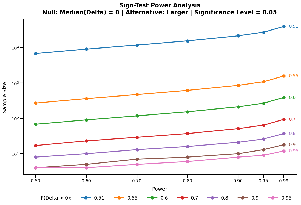
Figure 2: Test sample size $N$ vs. power $H_{N,\alpha}$ for $\alpha=5\%$ and several values of $p>1/2$.

The multiple testing problem can also be addressed in the randomized setting. A standard Bonferroni adjustment with test function $\phi_{N}(n,\alpha/d)$ and $p$-value being conditionally uniform on the interval $(da_{N}(n_{+})\wedge 1,db_{N}(n_{+})\wedge 1)$, where $d$ is the dimension of the feature vector, controls the family-wise error rate (FWER, the probability of having at least one false discovery), see kulinskaya2009fuzzy. For a less conservative approach, one can also control the False Discovery Rate [benjamini1995controlling]. kulinskaya2009fuzzy develop a formula and an algorithm for the adjusted rejection probability. habiger2015multiple proposes an alternative Monte Carlo approach. cousido2022multiple provide a comparison of methods, finding that the Monte Carlo approach outperforms its alternatives in terms of test power.

4 Measuring feature importance

We require measures of feature importance that complement the feature $p$-values delivered by our test. A local measure of feature importance is given by the feature effect $\Delta_{i}$, which represents the impact of a feature at the sample level. The median $M$ of the (conditional) feature effect distribution $F_{\Delta}$ is a natural measure of feature importance at the population level. Under Assumption 3.1, a consistent estimator of $M$ is the empirical median

$$\widehat{M}=\mbox{Median}\{\Delta_{i}:i\in I_{2}\},$$ (6)

which satisfies $\mathbb{P}(\widehat{M}<M)=\mathbb{P}(\widehat{M}>M)$ for odd $N=|I_{2}|$ and approximate equality holding for even $N$. Thus (6) is (approximately) as likely to overestimate $M$ as to underestimate it. Moreover, the distribution of $\widehat{M}$ is continuous. The estimator $\widehat{M}$ is unbiased if $F_{\Delta}$ is symmetric about $M$; see Section 4.4 of lehmann.

We construct one-sided, randomized confidence intervals (CIs) for $M$ by inverting the test (2). Let $\{\Delta_{(i)}\}$ denote the ordered sequence of $\{\Delta_{i}\}$; we take $\Delta_{(0)}=-\infty$ and $\Delta_{(N+1)}=\infty$. Let $\mathbb{P}_{M}$ denote the sampling distribution of the $\{\Delta_{i}\}$ when $M$ is the true median.

Proposition 4.1.

Let $U$ be an independent $U(0,1)$ variable. Define a randomized CI by

$$C_{N}(\alpha;U)=\begin{cases}[\Delta_{(N-T_{N,\alpha})},\infty),&1-\gamma_{N}(T_{N,\alpha},\alpha)\geq U\\ [\Delta_{(N-T_{N,\alpha}+1)},\infty),&\text{else}\end{cases}$$ (7)

where $T_{N,\alpha}=q_{1-\alpha}(B_{N,1/2})$ is the boundary of the test’s rejection region and $\gamma_{N}(n,\alpha)$ is the rejection probability (3). Under Assumption 3.1, the CI (7) has exact coverage:

$$\mathbb{P}_{M}(M\in C_{N}(\alpha;U))=1-\alpha,\quad\alpha\in(0,1).$$ (8)

In analogy to the randomized $p$-value, the randomized CI (7) inherits the exactness of the test’s decision rule (2). If $0<\Delta_{(N-T_{N,\alpha})}$ we reject the null for $M_{0}=0$. If $\Delta_{(N-T_{N,\alpha}+1)}\leq 0$ we retain the null. Else we reject with probability $\gamma_{N}(T_{N,\alpha},\alpha)$ (that is, draw a sample $u$ from $U(0,1)$ and reject if $u\leq\gamma_{N}(T_{N,\alpha},\alpha)$). In practice, it suffices to report the interval endpoints along with the rejection probability.

Figure 3: Rejection probability vs. CI endpoints.

Standard arguments lead to alternative two-sided CIs, which are not, however, dual to the test (2). Observe that $\mathbb{P}_{M}(\Delta_{(i)}\leq M\leq\Delta_{(i+1)})=\pi_{N}(i)$ for $i=0,1,\ldots,N$. Using these probabilities, we can combine intervals $(\Delta_{(i)},\Delta_{(i+1)})$ so as to attain a desired confidence coefficient. Choosing the intervals symmetrically, we obtain intervals

$$c_{m,N}=[\Delta_{(1+m)},\Delta_{(N-m)}]$$ (9)

satisfying $\mathbb{P}_{M}(M\in c_{m,N})=1-2\Pi_{N}(m)$, where we select $m\in\mathbb{N}$ so that $\Pi_{N}(m)\leq\alpha/2$ for given $\alpha\in(0,1)$. Then, $\mathbb{P}_{M}(M\in c_{m,N})\geq 1-\alpha$, implying a conservative approach. zielinski extend this argument using randomization, resulting in CIs with exact $(1-\alpha)$ coverage and minimum expected length. Alternative asymptotic CIs can be obtained by bootstrapping (e.g. efron and falk-kaufmann), empirical likelihood [chen-hall], sectioning [asmussen-glynn] and other methods.

We develop several useful properties of the population-level feature importance measure defined by the median $M$. To this end, let $Z=(X,Y)\sim\mathbb{P}$ where $\mathbb{P}$ denotes the population law from which the observed data points $Z_{i}$ are independently drawn. For concreteness, consider a model for estimating the conditional mean, and take $\mu(X)=\mathbb{E}(Y|X)$ and the score function $S$ as given. The (population) feature effect is given by $\Delta=S(\mu(\overline{X}),Y)-S(\mu(\underline{X}),Y)$ where $\underline{X}$ and $\overline{X}$ are suitable baseline and comparison features, respectively.

As discussed in Section 2.1, the selection of $\underline{X}$ and $\overline{X}$ offers some degrees of freedom. Consider the basic choice from Example 2.1,

$$\underline{X}=\mathbb{E}(X)\quad\text{and}\quad\overline{X}=(X^{1},\mathbb{E}(X^{2}),\ldots,\mathbb{E}(X^{d})),$$ (10)

where for convenience we assume, without loss of generality, feature $X^{1}$ is to be tested. First note that for the choice (10) and given $\mu$ and $S$, the feature effect $\Delta$ is completely determined by the marginal laws of the features and the joint law of the response $Y$ and $X^{1}$. Thus the feature dependence structure does not matter; the importance measure $M$ generated by (10) is robust to feature correlation. This is a remarkable property given the sensitivity of popular importance measures including SHAP and LOCO to correlation among features (e.g. verdinelli-wasserman). The correlation sensitivity induces a bias in these measures, which can lead to dubious importance rankings.

Next we explore the relationship between $M$ and conditional independence. candes2018panning, berrett, tansey2018holdout, janson, bellot and others develop tests for a conditional independence hypothesis of feature significance in the model-X knockoff setting of candes2018panning. We show that the hypothesis we test ($M\leq M_{0}=0$) is generally weaker than an alternative conditional independence hypothesis. Below, we use the notation $X^{-1}=(X^{2},\ldots,X^{d})$.

Proposition 4.2.

Under (10), if $Y\mathchoice{\mathrel{\hbox to0.0pt{$\displaystyle\perp$\hss}\mkern 2.0mu{\displaystyle\perp}}}{\mathrel{\hbox to0.0pt{$\textstyle\perp$\hss}\mkern 2.0mu{\textstyle\perp}}}{\mathrel{\hbox to0.0pt{$\scriptstyle\perp$\hss}\mkern 2.0mu{\scriptstyle\perp}}}{\mathrel{\hbox to0.0pt{$\scriptscriptstyle\perp$\hss}\mkern 2.0mu{\scriptscriptstyle\perp}}}X^{1}\,|\,X^{-1}$ then $\Delta=0$ almost surely.

Note that Proposition 4.2 extends to functions $\mu(X)$ other than $\mathbb{E}(Y|X)$ as long as $Y\mathchoice{\mathrel{\hbox to0.0pt{$\displaystyle\perp$\hss}\mkern 2.0mu{\displaystyle\perp}}}{\mathrel{\hbox to0.0pt{$\textstyle\perp$\hss}\mkern 2.0mu{\textstyle\perp}}}{\mathrel{\hbox to0.0pt{$\scriptstyle\perp$\hss}\mkern 2.0mu{\scriptstyle\perp}}}{\mathrel{\hbox to0.0pt{$\scriptscriptstyle\perp$\hss}\mkern 2.0mu{\scriptscriptstyle\perp}}}X^{1}|X^{-1}$ implies that $\mu(X)$ is independent of the first entry of $X$. The converse to Proposition 4.2 is not generally true. A simple counterexample is $\mu(X)=(X^{1}-\mathbb{E}(X^{1}))(X^{2}-\mathbb{E}(X^{2}))$, i.e., second-order significant variables. A special case where the converse does hold is a standard linear model

$$Y=\mu(X)+\epsilon,\;\text{where}\;\mu(X)=\beta\cdot X\;\text{and}\;\beta=(\beta^{1},...,\beta^{d})\in\mathbb{R}^{d}.$$ (11)

Before stating a converse of Proposition 4.2 under (11), we note the following “linear agreement” property: under (11) (and symmetry of the distribution of $\Delta$), the median $M$ measuring feature importance is proportional to the square of the regression coefficient, which is the canonical measure of feature importance in a linear model. The proportionality factor is given by the variance of the feature.

Proposition 4.3.

Consider the linear model (11). Select (10) and a standard score function $S(m,y)=-(m-y)^{2}$. If $\mathbb{E}(X^{-1}|X^{1})=\mathbb{E}(X^{-1})$ and $\mathbb{E}(\epsilon|X^{1})=0$, we have

$$\mathbb{E}(\Delta)=(\beta^{1})^{2}var(X^{1}).$$

Proposition 4.4.

Consider the linear model (11). Select (10) and a standard score function $S(m,y)=-(m-y)^{2}$. Suppose $\mathbb{E}(X^{-1}|X^{1})=\mathbb{E}(X^{-1})$, $var(X^{1})>0$ and $\epsilon\mathchoice{\mathrel{\hbox to0.0pt{$\displaystyle\perp$\hss}\mkern 2.0mu{\displaystyle\perp}}}{\mathrel{\hbox to0.0pt{$\textstyle\perp$\hss}\mkern 2.0mu{\textstyle\perp}}}{\mathrel{\hbox to0.0pt{$\scriptstyle\perp$\hss}\mkern 2.0mu{\scriptstyle\perp}}}{\mathrel{\hbox to0.0pt{$\scriptscriptstyle\perp$\hss}\mkern 2.0mu{\scriptscriptstyle\perp}}}X$. Then, $\Delta=0$ almost surely implies $Y\mathchoice{\mathrel{\hbox to0.0pt{$\displaystyle\perp$\hss}\mkern 2.0mu{\displaystyle\perp}}}{\mathrel{\hbox to0.0pt{$\textstyle\perp$\hss}\mkern 2.0mu{\textstyle\perp}}}{\mathrel{\hbox to0.0pt{$\scriptstyle\perp$\hss}\mkern 2.0mu{\scriptstyle\perp}}}{\mathrel{\hbox to0.0pt{$\scriptscriptstyle\perp$\hss}\mkern 2.0mu{\scriptscriptstyle\perp}}}X^{1}|X^{-1}$.

5 Synthetic tasks

This section illustrates the robust performance of our test and feature importance measure on synthetic “known truth” regression and classification tasks using neural networks. It also benchmarks performance against existing model-agnostic tests and variable selection procedures, as well as alternative model-specific and -agnostic feature importance measures.

5.1 Regression

We consider a feature vector $X=(X^{1},\ldots,X^{d})\subseteq\mathbb{R}^{d}$ of dimension $d=19$ and a response $Y\in\mathbb{R}$ of the form

$$Y=\mu(X)+\epsilon,\quad\epsilon\sim N(0,1),$$ (12)

where the error $\epsilon$ is independent of $X$ and the conditional mean function $\mu$ is given by

$$\mu(x)=3 +4x_{1}+x_{1}x_{2}+3x_{3}^{2}+2x_{4}x_{5}+6x_{6}+2\sin(x_{7})$$

$$+\exp(x_{8})+5x_{9}+3x_{10}+4x_{11}+5x_{12}.$$ (13)

The features $X_{1}$ and $X_{6}$ are jointly normal with mean zero, unit variances and covariances equal to $0.85$. The features $X_{2},\ldots,X_{5},X_{7}$ are independent $N(0,1)$, $X_{8}$ is uniform on $[-1,1]$, $X_{9}=1\{X_{2}+Z<0\}$ where $Z\sim N(0,1)$, $X_{10}$ is Poisson with mean 3 and $X_{11}$ and $X_{12}$ are independent variables with a $t$-distribution and 5 degrees of freedom. The non-influential variables $X_{13}$ and $X_{14}$ are independent $N(0,1)$, $(X_{15},X_{16})$ are jointly normal with mean zero, unit variances and covariances equal to $0.85$, and $X_{17},X_{18}$ and $X_{19}$ are independent variables with a $t$-distribution and 5 degrees of freedom.

We generate a training set $I_{1}$ of $10^{6}$ independent samples $(X_{i},Y_{i})$ and a test set $I_{2}$ of $5\cdot 10^{5}$ independent samples. We train a single-layer neural network model $f$ of the conditional mean $\mu(X)=\mathbb{E}(Y|X)$. Specifically,

$$f(x)=b_{0}+\sum_{k=1}^{K}b_{k}\psi(a_{0,k}+a_{k}^{\top}x),$$ (14)

where $K$ is the number of units, $\psi(y)=1/(1+e^{-y})$ is the activation function, and $b_{0},b_{k},a_{0,k}\in\mathbb{R}$ and $a_{k}\in\mathbb{R}^{d}$ are parameters to be estimated. The training procedure uses a standard $L_{2}$ loss criterion, $L_{2}$ regularization (of the weights $b_{k}$), the Adam optimization method, a batch size of 32, and 500 epochs with early stopping. We iterate across five random initializations. A validation set ($25\%$ of $I_{1}$, not used for training) and a Bayesian approach are used to optimize the regularization weight, the learning rate and the number of units, $K$. The optimal weight is $7\cdot 10^{-4}$, the optimal learning rate is $5\cdot 10^{-4}$ and the optimal $K=300$. The $R^{2}$ on the training (and test) data exceeds $99\%$.

The testing procedure uses a score function $S(m,y)=-(m-y)^{2}$ consistent with the $L_{2}$ training criterion. We use the basic baseline and comparison feature specifications discussed in Example 2.1. That is, for testing feature $\ell\in[d]$ we take

$$\underline{X}_{i} =(X^{1}_{i},\ldots,X^{\ell-1}_{i},v^{\ell}_{i},X^{\ell+1}_{i},\ldots,X^{d}_{i})$$

$$\overline{X}_{i} =X_{i}=(X_{i}^{1},\ldots,X^{d}_{i})$$ (15)

where $v^{\ell}_{i}$ is the mean of $\{X^{\ell}_{k}:k\in I_{1}\}$ in case feature $\ell$ is continuous. For the one-hot feature $\ell=9$, we use $v^{\ell}_{i}=1-X^{\ell}_{i}$ and for the Poisson feature $\ell=10$, we use the “alternative mode” $v^{\ell}_{i}={\arg\max}_{x\in\mathbb{N}\setminus\{X^{\ell}_{i}\}}p^{\ell}(x|I_{1})$ where $p^{\ell}(\cdot|I_{1})$ is the probability mass function of $\{X^{\ell}_{k}:k\in I_{1}\}$. The latter choice avoids baseline and comparison features being identical for too many samples, which is an issue arising with the standard mode. Our specifications yield baseline values in the support of $X^{9}$ and $X^{10}$.

$\ell$	AICO		CPT		HRT		LOCO		Deep		Gaussian
									Knockoff		Knockoff
	5%	1%	5%	1%	5%	1%	5%	1%	5%	1%	5%	1%
1	10	10	10	10	10	10	10	10	10	10	10	10
2	10	10	10	10	10	10	10	10	10	10	10	10
3	10	10	10	10	10	10	10	10	10	10	10	10
4	10	10	10	10	10	10	10	10	8	8	10	10
5	10	10	10	10	10	10	10	10	8	8	10	10
6	10	10	10	10	10	10	10	10	10	10	10	10
7	10	10	10	10	10	10	10	10	10	10	10	10
8	10	10	10	10	10	10	10	10	9	9	10	10
9	10	10	10	10	10	10	10	10	10	10	10	10
10	10	10	10	10	10	10	10	10	10	10	10	10
11	10	10	10	10	10	10	10	10	10	10	10	10
12	10	10	10	10	10	10	10	10	10	10	10	10
13	0	0	3	2	0	0	0	0	3	3	4	4
14	0	0	1	1	1	1	1	1	2	2	3	3
15	0	0	2	2	0	0	0	0	0	0	4	4
16	0	0	4	4	1	1	0	0	1	1	3	3
17	0	0	0	0	1	1	1	0	2	2	3	3
18	0	0	0	0	1	1	0	0	0	0	2	2
19	0	0	1	0	0	0	0	0	0	0	2	2

Table 1: Regression model test results for 10 independent training/testing experiments at two standard confidence levels ($\alpha=5\%$ and $\alpha=1\%$). The table compares AICO, CPT, HRT, LOCO, Deep Knockoff, and Gaussian Knockoff procedures, showing the total number of rejections across 10 trials. The test set size is $N=5\cdot 10^{5}$.

We run 10 independent training/testing experiments to assess the behavior of the test. The second and third columns of Table 1 report the results for confidence levels $\alpha=0.01$ and $0.05$. The test has perfect power and does not produce false discoveries. Feature correlation (e.g. $\ell=1,6$) and discrete feature distributions ($\ell=9,10$) do not affect performance. The test also correctly detects the significance of features $\ell=2,4,5$ which influence the response only through product terms. Additional experiments show robustness to alternative baseline specifications (e.g. taking $v^{\ell}_{i}$ as the training mean also for the discrete features $\ell=9,10$, and using the median instead of the mean to construct $v^{\ell}_{i}$). We also verify robustness with respect to the score function $S$ including the alternative specification $S(m,y)=-|m-y|$.

We contrast our test with recently developed model-agnostic alternatives, including the Leave-Out-Covariates Test (LOCO) of Lei2018predictive, the Conditional Permutation Test (CPT) of berrett, and the Holdout Randomization Test (HRT) of tansey2018holdout. LOCO tests the mean or median delta in $L_{2}$ model loss $(Y_{i}-f^{-\ell}(X^{-\ell}_{i}))^{2}-(Y_{i}-f(X_{i}))^{2}$ across the test set $I_{2}$ due to removing feature $\ell$ from $X$. Specifically, $X^{-\ell}_{i}$ represents the $i$th sample feature value without the $\ell$th component and $f^{-\ell}$ represents a neural network model (14) trained on $\{(Y_{i},X^{-\ell}_{i}):i\in I_{1}\}$. Testing all features requires re-training the model (14) $d=19$ times, each time for a different feature set. This approach entails a significant additional computational expense that our testing procedure avoids.

The CPT and HRT tests are based on the Conditional Randomization Test of candes2018panning, which is computationally challenging. They test the conditional independence hypothesis $Y\mathchoice{\mathrel{\hbox to0.0pt{$\displaystyle\perp$\hss}\mkern 2.0mu{\displaystyle\perp}}}{\mathrel{\hbox to0.0pt{$\textstyle\perp$\hss}\mkern 2.0mu{\textstyle\perp}}}{\mathrel{\hbox to0.0pt{$\scriptstyle\perp$\hss}\mkern 2.0mu{\scriptstyle\perp}}}{\mathrel{\hbox to0.0pt{$\scriptscriptstyle\perp$\hss}\mkern 2.0mu{\scriptscriptstyle\perp}}}X^{\ell}\,|\,X^{-\ell}$ where $X^{-\ell}=(X^{1},\ldots,X^{\ell-1},X^{\ell+1},\ldots,X^{d})$. The tests require sampling from the (unknown) conditional law of $X^{\ell}$ given $X^{-\ell}$. We follow tansey2018holdout and construct $d=19$ mixture density neural networks for the conditional laws. For additional perspective, we also implement recent model-agnostic variable selection procedures, including the Gaussian Model-X Knockoff procedure of candes2018panning and the Deep Model-X Knockoff procedure of deepknockoffs. The former relies on a Gaussian model of the feature distribution while the latter constructs a deep neural network for sampling from the feature distribution. The construction of complex auxiliary models in the CPT, HRT and knockoff procedures entails a significant additional computational expense that our AICO approach avoids.

Table 1 reports the results of the aforementioned alternative procedures for 10 independent training/testing experiments. CPT, HRT and LOCO deliver the same power as AICO but come with an increased false discovery rate (some but not all of these false discoveries can be addressed by a standard Bonferroni correction). The Gaussian Knockoff procedure selects the significant features 1 through 12 in each independent experiment. However, it does generate some false discoveries (which is consistent with control of the expected false discovery rate). The Deep Knockoff procedure reduces false discoveries at the expense of lower power. This approach has slight difficulty identifying the features entering the model (5.1) through the product term $2x_{4}x_{5}$.

We consider the performance of our AICO test as a function of the size $N=|I_{2}|$ of the test set. Table 2 reports the results for $N\in\{10^{5},10^{4},10^{3},500,100\}$; the case $N=5\cdot 10^{5}$ is reported in Table 1. The test offers maximum power even for $N$ as small as 500. The power deteriorates moderately for smaller $N$; false discoveries rise only very slowly. This validates the performance of the test even for small samples.

AICO
$\ell$	$N=10^{5}$		$N=10^{4}$		$N=10^{3}$		$N=500$		$N=250$		$N=100$
	5%	1%	5%	1%	5%	1%	5%	1%	5%	1%	5%	1%
1	10	10	10	10	10	10	10	10	10	10	10	10
2	10	10	10	10	10	10	10	10	10	9	8	5
3	10	10	10	10	10	10	10	10	10	10	10	10
4	10	10	10	10	10	10	10	10	10	10	9	9
5	10	10	10	10	10	10	10	10	10	10	10	9
6	10	10	10	10	10	10	10	10	10	10	10	10
7	10	10	10	10	10	10	10	10	10	10	10	10
8	10	10	10	10	10	10	10	10	9	8	8	7
9	10	10	10	10	10	10	10	10	10	10	10	10
10	10	10	10	10	10	10	10	10	10	10	10	10
11	10	10	10	10	10	10	10	10	10	10	10	10
12	10	10	10	10	10	10	10	10	10	10	10	10
13	0	0	0	0	0	0	0	0	2	1	0	0
14	0	0	0	0	0	0	1	0	0	0	1	0
15	0	0	1	0	1	1	0	0	1	0	1	0
16	0	0	0	0	0	0	1	1	0	0	1	0
17	1	0	0	0	1	0	0	0	0	0	0	0
18	0	0	1	0	0	0	0	0	0	0	0	0
19	0	0	1	0	0	0	0	0	0	0	2	2

Table 2: Regression model test results for 10 independent training/testing experiments, evaluated at two confidence levels ($\alpha=5\%$ and $1\%$) for several test sample sizes $N$. We report the number of times the null was rejected out of 10 trials for each covariate $\ell\in[d]$.

We turn to measuring feature importance. Table 3 provides a feature importance ranking according to the empirical median (6) for one of the 10 independent training/testing experiments that was randomly chosen. It also reports the endpoints of the randomized CI (7) for the population median $M$ at a $99\%$ level, and the standard (non-randomized) two-sided CI (9) along with coverage probabilities. Table 3 also provides the distribution of the randomized $p$-value.

AICO, Level $\alpha=1\%$
				$p$-value Distribution		Randomized One-Sided CI			Non-Randomized Two-Sided CI
Rank	Feature	Median	P(Reject)	Lower	Upper	98.8%	1.2%	Coverage	Lower	Upper	Coverage
1	$X_{9}$	24.993	1.000	0.000	0.000	24.951	24.951	0.99	24.947	25.040	0.99007
2	$X_{6}$	15.788	1.000	0.000	0.000	15.661	15.661	0.99	15.647	15.938	0.99007
3	$X_{10}$	14.572	1.000	0.000	0.000	14.511	14.511	0.99	14.506	14.640	0.99007
4	$X_{12}$	12.898	1.000	0.000	0.000	12.789	12.789	0.99	12.775	13.022	0.99007
5	$X_{11}$	8.137	1.000	0.000	0.000	8.063	8.063	0.99	8.054	8.218	0.99007
6	$X_{1}$	6.210	1.000	0.000	0.000	6.155	6.155	0.99	6.148	6.273	0.99007
7	$X_{3}$	1.697	1.000	0.000	0.000	1.669	1.669	0.99	1.666	1.730	0.99007
8	$X_{7}$	0.953	1.000	0.000	0.000	0.941	0.941	0.99	0.940	0.964	0.99007
9	$X_{4}$	0.416	1.000	0.000	0.000	0.409	0.409	0.99	0.409	0.424	0.99007
10	$X_{5}$	0.416	1.000	0.000	0.000	0.409	0.409	0.99	0.408	0.424	0.99007
11	$X_{8}$	0.143	1.000	0.000	0.000	0.140	0.140	0.99	0.139	0.146	0.99007
12	$X_{2}$	0.084	1.000	0.000	0.000	0.082	0.082	0.99	0.082	0.086	0.99007
-	$X_{13}$	-1.154e-07	0.000	0.880	0.881	-2.442e-06	-2.437e-06	0.99	-2.708e-06	1.478e-06	0.99007
-	$X_{14}$	-2.054e-07	0.000	0.928	0.928	-2.176e-06	-2.175e-06	0.99	-2.389e-06	9.014e-07	0.99007
-	$X_{15}$	-3.060e-07	0.000	0.845	0.846	-3.339e-06	-3.338e-06	0.99	-3.639e-06	2.127e-06	0.99007
-	$X_{16}$	-5.512e-07	0.000	0.937	0.937	-2.966e-06	-2.965e-06	0.99	-3.275e-06	9.626e-07	0.99007
-	$X_{17}$	-1.340e-06	0.000	0.996	0.997	-3.773e-06	-3.773e-06	0.99	-4.022e-06	0.000	0.99150
-	$X_{18}$	0.000	0.000	0.860	0.861	-1.426e-06	-1.423e-06	0.99	-1.634e-06	1.114e-06	0.99007
-	$X_{19}$	0.000	0.000	0.815	0.816	-1.517e-06	-1.516e-06	0.99	-1.716e-06	1.333e-06	0.99007

Table 3: Regression model feature importance ranking according to the empirical median (6) for one of the independent training/testing experiments that was randomly chosen. The table also reports the endpoints of the randomized CI (7) for the median at a $99\%$ level, the standard (non-randomized) two-sided CI (9) along with coverage probabilities, and the distribution of the randomized $p$-value.

The $p$-value distributions show that our approach is able to clearly distinguish between the significant and irrelevant features. The distributions of the significant features $\ell=1,\ldots,12$ are concentrated near 0, far below the level $\alpha=1\%$. This provides substantial evidence in favor of rejecting the null for these features (the rejection probability is equal to 1). The $p$-value distributions of the irrelevant features are concentrated significantly above $\alpha$, implying clear retention of the null for these features. There are no equivocal cases, eliminating the need to actually randomize.

Feature $\ell=9$ is judged to be the most important feature, followed by features $\ell=6,10$ and $12$. The remaining significant features are relatively less important compared with this group of variables. Features $\ell=4,5$ have (almost) identical medians and CIs and thus importance, consistent with their symmetric roles in the conditional mean function (5.1).

To demonstrate the stability of AICO feature importance scores, Figure 4 shows the empirical median (6) for each of the ten training/testing experiments. The AICO importance ranking is stable and robust to noise in the data. The ranking is also robust to alternative choices of the score function $S$ such as $S(m,y)=-|m-y|$ (results available upon request). For comparison, Figure 4 also provides test-implied feature importance scores for CPT, HRT, and LOCO [berrett, tansey2018holdout, verdinelli-wasserman], kernel and deep SHAP feature importance [lundberg2017unified], permutation feature importance scores [breiman, fisher-rudin], and Gaussian and deep knockoff feature importance scores [candes2018panning, deepknockoffs]. It is important to note that there is no ground truth for feature importance [hama-mase-owen]; hence we do not focus on the differences in importance rankings across alternative approaches. We do, however, highlight the robustness of the measures based on testing and variable selection procedures. The widely-used SHAP measures deliver inconsistent rankings across implementations (deep vs. kernel). The rankings are also highly unstable across experiments (data sets). That is, they appear to be highly susceptible to noise in the data. This questions the usefulness of SHAP for feature importance.

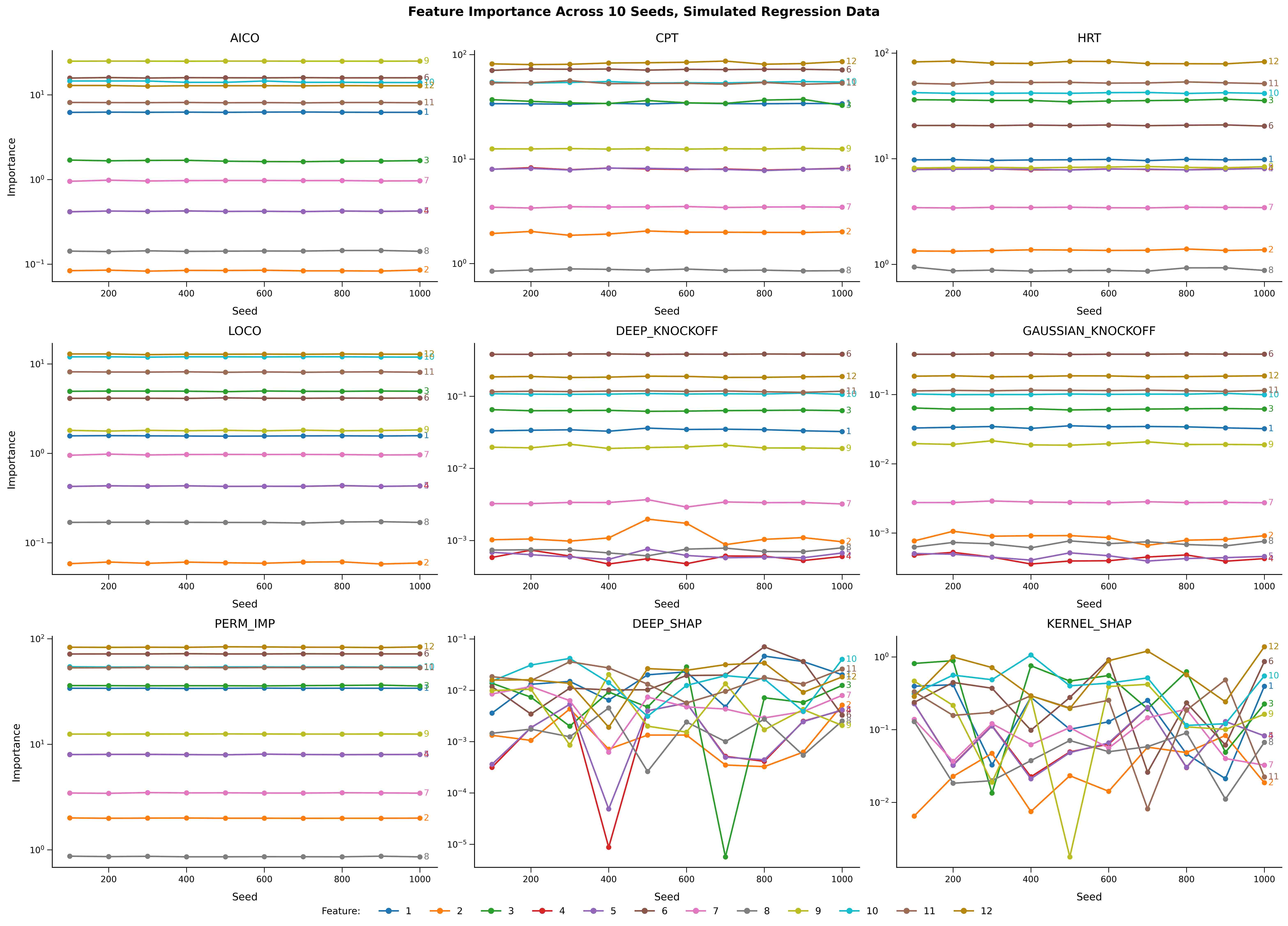
Figure 4: Feature importance scores across training/testing experiments.

Finally we consider the computational efficiency of our test vs. the aforementioned alternatives. Figure 5 reports average computation times across 10 experiments. In each of these experiments we test (AICO, CPT, HRT, LOCO) or screen (knockoffs) all 19 features or, in the case of SHAP and permutation feature importance, compute importance scores for all 19 features. The time reported includes the time to train any sub or auxiliary models. It does not include the time to train the original neural network (14).

AICO achieves an unprecedented degree of computational efficiency. In terms of full-fledged testing procedures, AICO is more than three orders of magnitude faster than LOCO, the next most efficient testing procedure. AICO is almost two orders of magnitudes more efficient than Gaussian knockoffs, the fastest screening procedure. It is more than three orders of magnitude faster than permutation importance, the fastest algorithmic feature importance measure. The testing results reported earlier in this section demonstrate that AICOs computational efficiency does not come at the expense of statistical performance.

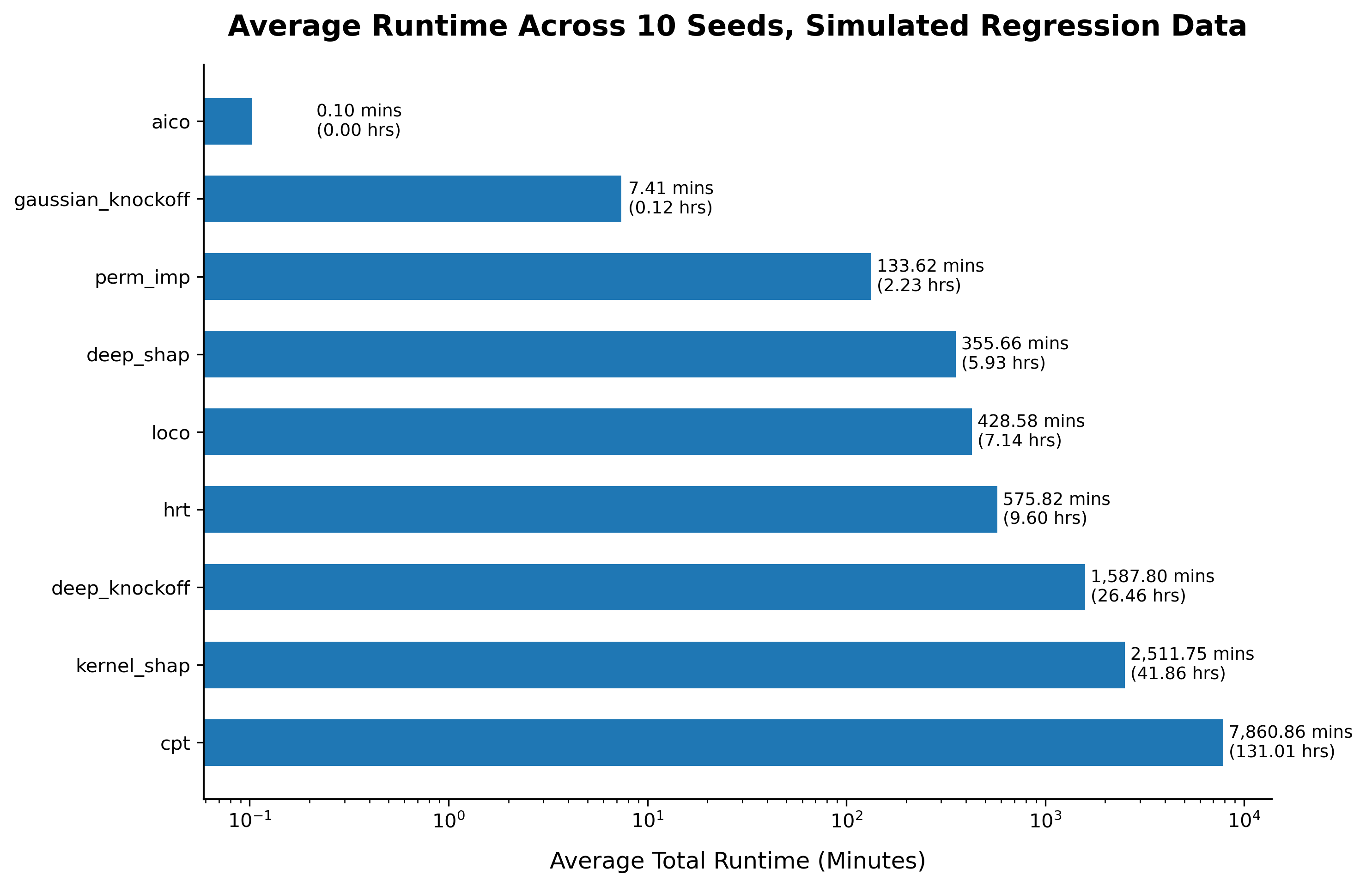
Figure 5: Average computation times for testing/screening all 19 features.

5.2 Classification

We next consider a binary response $Y\in\{0,1\}$ governed by the model

$$\mathbb{E}(Y|X)=\mathbb{P}(Y=1|X)=L(\mu(X))$$ (16)

where $L(u)=1/(1+e^{u})$, the function $\mu$ is given by (5.1) and the features $X=(X^{1},\ldots,X^{d})$ are as defined in Section 5.1. We generate a training set $I_{1}$ of $10^{6}$ independent samples $(X_{i},Y_{i})$ and a test set $I_{2}$ of $5\cdot 10^{5}$ independent samples. The data are imbalanced, as is often the case in practice (e.g. credit scoring): about $10\%$ of the samples have $Y_{i}=1$. We train a single-layer neural network model $f$ of the conditional mean $\mathbb{E}(Y|X)$:

$$f(x)=L\left(b_{0}+\sum_{k=1}^{K}b_{k}\psi(a_{0,k}+a_{k}^{\top}x)\right)$$ (17)

where $\psi(y)=1/(1+e^{-y})$, $K$ is the number of units, and $b_{0},b_{k},a_{0,k}\in\mathbb{R}$ and $a_{k}\in\mathbb{R}^{d}$ are parameters. The training procedure uses a standard cross-entropy criterion, $L_{2}$ regularization with weight $10^{-3}$ (approximately the optimal weight in the regression model training), Adam, a batch size of 32, and 500 epochs with early stopping. A validation set ($25\%$ of $I_{1}$) and a Bayesian approach are used to optimize the learning rate and the number of units, $K$. The optimal learning rate is $5\cdot 10^{-4}$ and the optimal $K=300$. The Area Under the ROC Curve on the training (and test) data exceeds $99\%$.

The testing procedure employs a score function $S(m,y)=y\log m+(1-y)\log(1-m)$ consistent with the training criterion. We use the baseline and comparison feature specification (5.1). Table 4 reports the results for confidence levels $\alpha=0.01,0.05$. As in the regression case, the test has perfect power and avoids false discoveries. The test is generally robust to alternative specifications of the baseline (e.g. using the median instead of the mean to construct $v^{\ell}$, setting $v^{\ell}$ to the training mean also for the 1-hot feature $\ell=9$). The test is also robust to using an alternative score function $S(m,y)=-(m-y)^{2}$.

$\ell$	AICO		CPT		HRT		LOCO		Deep		Gaussian
									Knockoff		Knockoff
	5%	1%	5%	1%	5%	1%	5%	1%	5%	1%	5%	1%
1	10	10	10	10	9	9	10	10	10	10	10	10
2	10	10	10	10	9	9	10	10	10	10	10	10
3	10	10	10	10	9	9	10	10	10	10	10	10
4	10	10	10	10	9	9	10	10	9	9	10	10
5	10	10	10	10	9	9	10	10	10	10	9	9
6	10	10	10	10	9	9	10	10	10	10	10	10
7	10	10	10	10	9	9	10	10	10	10	10	10
8	10	10	10	10	9	9	10	10	9	9	9	9
9	10	10	10	10	9	9	10	10	10	10	10	10
10	10	10	10	10	9	9	10	10	10	10	6	6
11	10	10	10	10	9	9	10	10	10	10	10	10
12	10	10	10	10	9	9	10	10	10	10	10	10
13	1	1	1	1	2	2	4	4	2	2	1	1
14	0	0	2	1	0	0	5	5	1	1	1	1
15	0	0	2	2	4	4	6	6	0	0	3	3
16	0	0	3	1	2	2	5	5	1	1	2	2
17	1	1	0	0	1	1	5	5	0	0	1	1
18	1	1	0	0	3	3	5	5	0	0	2	2
19	1	1	1	1	1	1	3	3	0	0	1	1

Table 4: Classification model test results for 10 independent training/testing experiments at two standard confidence levels ($\alpha=5\%$ and $\alpha=1\%$). The table compares AICO, LOCO, HRT, Deep Knockoff, and Gaussian Knockoff procedures, showing the total number of rejections across 10 trials. The test set size is $N=5\cdot 10^{5}$.

Table 4 also reports the results for LOCO, CPT, HRT and Gaussian and deep knockoff procedures. AICO, CPT and LOCO have full power. LOCO, however, suffers from significant number of false discoveries (which cannot be addressed with a standard Bonferroni adjustment). HRT and knockoff procedures have less power and some false discoveries. In this comparison, AICO outperforms the alternatives. It performs as well as in the regression setting.

AICO
$\ell$	$N=10^{5}$		$N=10^{4}$		$N=10^{3}$		$N=500$		$N=250$		$N=100$
	5%	1%	5%	1%	5%	1%	5%	1%	5%	1%	5%	1%
1	10	10	10	10	10	10	10	10	9	7	3	0
2	10	10	10	10	6	5	3	2	6	5	3	1
3	10	10	10	10	10	10	10	10	10	10	8	8
4	10	10	10	10	10	10	10	9	6	2	4	0
5	10	10	10	10	10	10	8	8	8	6	6	1
6	10	10	10	10	10	10	10	10	8	6	2	1
7	10	10	8	7	3	3	2	0	1	0	0	0
8	10	10	5	2	0	0	0	0	0	0	0	0
9	10	10	10	10	6	3	3	1	5	3	3	1
10	10	10	10	10	10	10	10	10	9	9	8	5
11	10	10	10	10	6	2	9	5	0	0	3	1
12	10	10	10	10	10	9	6	5	5	2	2	0
13	0	0	1	0	1	0	3	0	0	0	0	0
14	0	0	0	0	0	0	1	0	1	0	2	1
15	0	0	0	0	0	0	0	0	1	1	1	0
16	0	0	0	0	0	0	0	0	0	0	2	0
17	1	1	1	0	1	0	2	0	0	0	0	0
18	1	1	1	0	1	0	2	0	0	0	0	0
19	0	0	1	0	1	0	0	0	0	0	0	0

Table 5: Classification model test results for 10 independent training/testing experiments, at two confidence levels ($\alpha=5\%$ and $\alpha=1\%$), across various test sample sizes $N$. We report the total number of rejections over 10 trials.

Table 5 reports test results for varying test set sample sizes $N$. Power decreases faster with $N$ than in the regression case, especially for features $\ell=7,8$. False discoveries appear to be fairly insensitive to $N$.

AICO, Level $\alpha=1\%$
				P-Value Distribution		Randomized One-Sided CI			Non-Randomized Two-Sided CI
rank	variable	median	P(reject)	lower	upper	98.8%	1.2%	coverage	lower	upper	coverage
1	$X_{3}$	3.577e-07	1.000	0.000	0.000	3.340e-07	3.340e-07	0.99	3.320e-07	3.829e-07	0.99007
2	$X_{10}$	2.324e-08	1.000	0.000	0.000	2.077e-08	2.077e-08	0.99	2.053e-08	2.619e-08	0.99007
3	$X_{6}$	6.722e-10	1.000	0.000	0.000	6.014e-10	6.016e-10	0.99	5.939e-10	7.656e-10	0.99007
4	$X_{1}$	1.630e-10	1.000	0.000	0.000	1.442e-10	1.443e-10	0.99	1.426e-10	1.862e-10	0.99007
5	$X_{12}$	6.989e-11	1.000	0.000	0.000	5.826e-11	5.828e-11	0.99	5.702e-11	8.597e-11	0.99007
6	$X_{5}$	4.339e-11	1.000	0.000	0.000	3.697e-11	3.697e-11	0.99	3.643e-11	5.135e-11	0.99007
7	$X_{4}$	3.169e-11	1.000	0.000	0.000	2.707e-11	2.707e-11	0.99	2.668e-11	3.733e-11	0.99007
8	$X_{11}$	1.001e-11	1.000	0.000	0.000	8.027e-12	8.030e-12	0.99	7.821e-12	1.275e-11	0.99007
9	$X_{9}$	6.787e-12	1.000	0.000	0.000	5.025e-12	5.025e-12	0.99	4.863e-12	9.439e-12	0.99007
10	$X_{2}$	2.575e-14	1.000	0.000	0.000	1.823e-14	1.825e-14	0.99	1.755e-14	3.704e-14	0.99007
11	$X_{7}$	1.100e-15	1.000	3.262e-71	3.431e-71	5.257e-16	5.261e-16	0.99	4.808e-16	2.326e-15	0.99007
12	$X_{8}$	1.344e-17	1.000	1.706e-14	1.743e-14	2.386e-18	2.394e-18	0.99	1.972e-18	4.921e-17	0.99007
-	$X_{13}$	0.000	0.000	1.000	1.000	0.000	0.000	0.99	0.000	0.000	1.00000
-	$X_{14}$	0.000	0.000	1.000	1.000	-1.396e-21	-1.390e-21	0.99	-2.680e-21	0.000	0.99485
-	$X_{15}$	-3.193e-21	0.000	1.000	1.000	-5.676e-20	-5.672e-20	0.99	-7.258e-20	0.000	0.99503
-	$X_{16}$	0.000	0.000	1.000	1.000	-3.066e-22	-3.052e-22	0.99	-5.372e-22	0.000	0.99501
-	$X_{17}$	0.000	0.000	1.000	1.000	0.000	0.000	0.99	0.000	0.000	0.99992
-	$X_{18}$	0.000	0.000	0.940	0.940	0.000	0.000	0.99	-1.849e-32	1.780e-22	0.99007
-	$X_{19}$	0.000	0.000	1.000	1.000	0.000	0.000	0.99	0.000	0.000	0.99999

Table 6: Classification model feature importance ranking according to the empirical median (6) for one of the independent training/testing experiments that was randomly chosen. The table also reports the endpoints of the randomized CI (7) for the median at a $99\%$ level, the standard (non-randomized) two-sided CI (9) along with coverage probabilities, and the distribution of the randomized $p$-value.

Table 6 provides a feature importance ranking according to the empirical median (6) for one of the 10 independent training/testing experiments that was randomly chosen. It also reports the endpoints of the randomized CI (7) for the population median $M$ at a $99\%$ level, and the standard (non-randomized) two-sided CI (9) along with coverage probabilities. Table 3 also provides the distribution of the randomized $p$-value.

Figure 6 shows the empirical median (6) for each of the ten training/testing experiments, for each of several methods including AICO. Across methods, the scores of the less important variables tend to be (somewhat) more volatile than in the regression setting. SHAP delivers inconsistent and highly unstable rankings, as in the regression case.

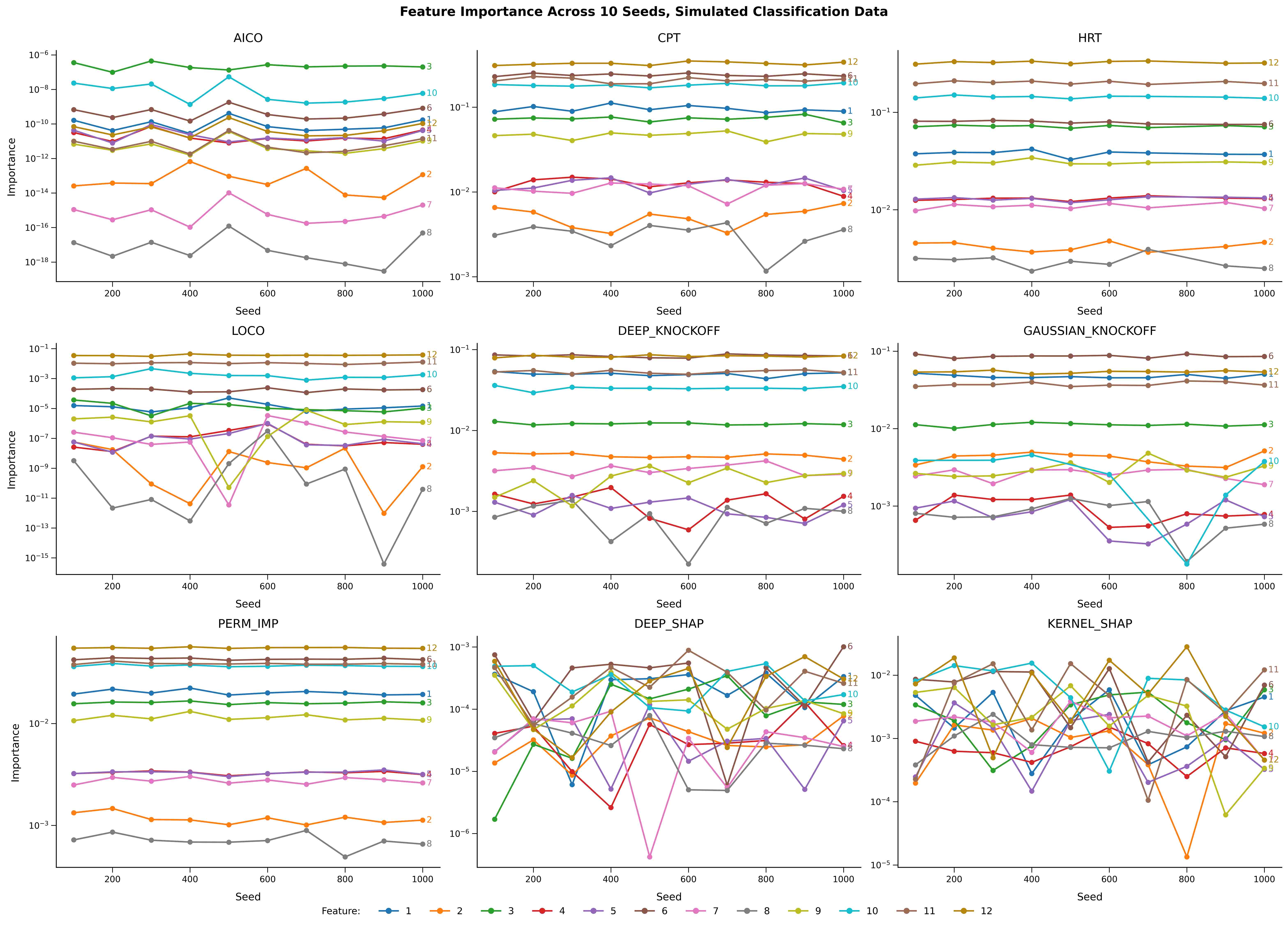
Figure 6: Classification model feature importance across training/testing experiments.

Figure 7 reports average computation times across 10 experiments. As in the regression case, AICO achieves an unprecedented degree of computational efficiency. It is more than three orders of magnitude faster than LOCO, the next most efficient testing procedure. AICO is an order of magnitude more efficient than Gaussian knockoffs, the fastest screening procedure. It is more than three orders of magnitude faster than permutation importance, the fastest algorithmic feature importance measure.

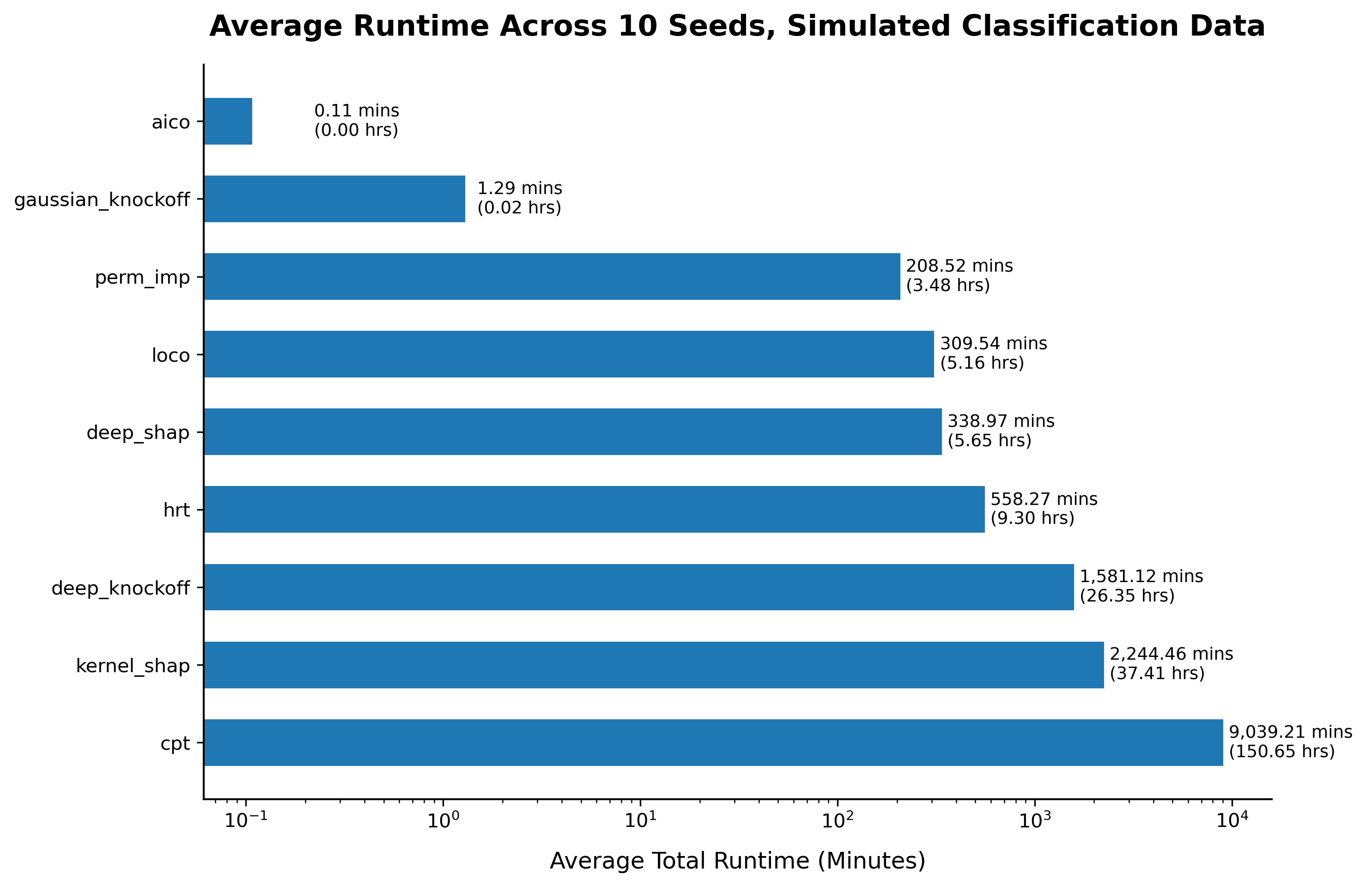
Figure 7: Average computation times for testing/screening all 19 features.

6 Empirical applications

6.1 Credit card default

This section complements our theoretical and numerical results with an empirical application to credit card payment data from 30,000 credit card holders of a Taiwanese card issuer, collected in October 2005. The response variable is a binary indicator of payment default. There are 23 explanatory variables (see Table 7). The dataset was split into training (60%), validation (15%), and testing (25%) sets with class proportions maintained through stratified sampling. Categorical variables are one-hot encoded and continuous variables are standardized (mean 0 and unit variance) based on training set statistics.

Feature	Data Type	Levels (for Categorical)	Description
LIMIT_BAL	Continuous	–	Amount of the given credit (NT dollars).
SEX	Categorical	Male, Female	Gender of the cardholder.
EDUCATION	Categorical	Graduate school, University, High school, Others	Education level of the cardholder.
MARRIAGE	Categorical	Married, Single, Others	Marital status of the cardholder.
AGE	Continuous	–	Age of the cardholder (in years).
PAY_0	Categorical	Paid in full, 1 Month delinquent, $\hskip 50.0pt\vdots$ 8 Months delinquent 9+ Months delinquent	Repayment status in September 2005.
PAY_2	Categorical	Same as PAY_0	Repayment status in August 2005.
PAY_3	Categorical	Same as PAY_0	Repayment status in July 2005.
PAY_4	Categorical	Same as PAY_0	Repayment status in June 2005.
PAY_5	Categorical	Same as PAY_0	Repayment status in May 2005.
PAY_6	Categorical	Same as PAY_0	Repayment status in April 2005.
BILL_AMT1	Continuous	–	Amount of bill statement (NT dollars) in September 2005.
BILL_AMT2	Continuous	–	Amount of bill statement (NT dollars) in August 2005.
BILL_AMT3	Continuous	–	Amount of bill statement (NT dollars) in July 2005.
BILL_AMT4	Continuous	–	Amount of bill statement (NT dollars) in June 2005.
BILL_AMT5	Continuous	–	Amount of bill statement (NT dollars) in May 2005.
BILL_AMT6	Continuous	–	Amount of bill statement (NT dollars) in April 2005.
PAY_AMT1	Continuous	–	Amount paid (NT dollars) in September 2005.
PAY_AMT2	Continuous	–	Amount paid (NT dollars) in August 2005.
PAY_AMT3	Continuous	–	Amount paid (NT dollars) in July 2005.
PAY_AMT4	Continuous	–	Amount paid (NT dollars) in June 2005.
PAY_AMT5	Continuous	–	Amount paid (NT dollars) in May 2005.
PAY_AMT6	Continuous	–	Amount paid (NT dollars) in April 2005.

Table 7: Raw features of the credit default dataset.

We implement an XGBoost [chen2016xgboost] classifier using a cross-entropy loss function. We use the area under the ROC curve (AUC) on the validation set as a metric for hyper-parameter optimization. We employ the Optuna package [akiba2019optuna], utilizing the Tree-Structured Parzen Estimator [bergstra2011algorithms], with 250 trials. The search space includes the boosting algorithm, tree-specific settings such as tree depth and minimum child weight, and regularization terms. Class imbalance was mitigated using a scaling weight parameter, and training was capped at 1,000 boosting rounds with early stopping if the validation AUC did not improve for 50 consecutive rounds. The optimal hyper-parameters include a gradient tree boosting algorithm [friedman2001greedy] with an approximation-based tree-building strategy; an L2 regularization parameter (lambda) of 0.2 and an L1 regularization parameter (alpha) of 0.001; a subsampling ratio of 100% (no subsampling); a column sampling ratio for each tree of 65%; a maximum tree depth of six levels; a minimum child weight of two; a learning rate (eta) of 0.05; a minimum loss reduction (gamma) of 0.00004; and a loss-guided tree growth policy.

We train an ensemble of 100 XGBoost models on 100 bootstrap samples of the training data, all using the same hyper-parameters obtained during the tuning phase. Each model was trained for up to 1,000 boosting rounds, with early stopping triggered after 50 rounds of no improvement in the validation AUC. Ensemble predictions are obtained by averaging the outputs of all 100 models. The resulting ensemble model has AUCs of $0.837$ on the training set, $0.782$ on the validation set, and $0.786$ on the test set. (The results are robust with respect to the model. An ensemble of neural networks, for example, yields very similar results.)

As in the classification example of Section 5.2, we use a score function $S(m,y)=y\log m+(1-y)\log(1-m)$ to run the test. We continue to use the baseline and comparison feature specification (5.1), where $v^{\ell}_{i}$ is the mean of $\{X^{\ell}_{k}:k\in I_{1}\}$ in case feature $\ell$ is continuous. For a categorical variable we take the alternative mode $v_{i}^{\ell}=\arg\max_{x\in\mathcal{X}^{\ell}\setminus\{X_{i}^{\ell}\}}p^{\ell}(x|I_{1})$ where $\mathcal{X}^{\ell}$ is the (marginal) support of $X^{\ell}$ and $p^{\ell}(\cdot|I_{1})$ is the (empirical) probability mass function of $\{X^{\ell}_{k}:k\in I_{1}\}$. This specification yields values in the support of a categorical. Here, we treat a categorical variable as a single feature rather than treating the associated one-hot variables separately. Alternatively, if higher resolution is required, we can run the test for each individual level of a categorical.

Table 8 summarizes the test results for $\alpha=1\%$ ($N=7,500$ throughout). The significant features, ranked according to the empirical median (6), are PAY_0 through PAY_6, MARRIAGE, SEX, and AGE. Past delinquencies are significant predictors of future payment default. The more recent the payment record the stronger is the influence of timely payment. The actual monthly bill and payment amounts (e.g., PAY_AMT and BILL_AMT) are not significant. Marital status, gender and age, but not education level, are significant predictors of default, even after controlling for past payment behavior. However, the influence of these variables is relatively small, especially for age (the associated medians are at least an order of magnitude smaller than the medians of the payment records). These results indicate that personal circumstances have a statistically significant influence on borrower behavior, beyond patterns in prior payment.

AICO, Level $\alpha=1\%$
				P-Value Distribution		Randomized One-Sided CI			Non-Randomized Two-Sided CI
rank	variable	median	P(reject)	lower	upper	23.4%	76.6%	coverage	lower	upper	coverage
1	PAY_0	0.150	1.000	0.000	0.000	0.143	0.143	0.99	0.142	0.155	0.99063
2	PAY_2	0.121	1.000	0.000	0.000	0.117	0.117	0.99	0.116	0.125	0.99063
3	PAY_3	0.095	1.000	0.000	0.000	0.091	0.091	0.99	0.091	0.099	0.99063
4	PAY_4	0.059	1.000	0.000	0.000	0.055	0.055	0.99	0.054	0.064	0.99063
5	PAY_5	0.037	1.000	2.520e-322	6.423e-322	0.035	0.035	0.99	0.035	0.039	0.99063
6	PAY_6	0.030	1.000	1.020e-297	2.493e-297	0.029	0.029	0.99	0.029	0.032	0.99063
7	MARRIAGE	0.002	1.000	3.912e-11	4.561e-11	0.002	0.002	0.99	0.001	0.003	0.99063
8	SEX	0.002	1.000	1.026e-37	1.383e-37	0.001	0.002	0.99	0.001	0.002	0.99063
9	AGE	3.796e-04	1.000	1.788e-09	2.056e-09	2.200e-04	2.204e-04	0.99	2.036e-04	5.814e-04	0.99063
-	LIMIT_BAL	0.000	0.000	0.794	0.800	0.000	0.000	0.99	0.000	3.603e-04	0.99496
-	BILL_AMT1	-0.006	0.000	1.000	1.000	-0.007	-0.007	0.99	-0.008	-0.005	0.99063
-	BILL_AMT2	-0.001	0.000	1.000	1.000	-0.002	-0.002	0.99	-0.002	-9.540e-04	0.99063
-	BILL_AMT3	0.000	0.000	0.975	0.976	-1.599e-04	-1.592e-04	0.99	-1.751e-04	5.542e-05	0.99063
-	BILL_AMT4	-4.094e-04	0.000	1.000	1.000	-5.298e-04	-5.284e-04	0.99	-5.504e-04	-2.773e-04	0.99063
-	BILL_AMT5	-3.203e-04	0.000	1.000	1.000	-5.070e-04	-5.054e-04	0.99	-5.220e-04	-1.887e-04	0.99063
-	BILL_AMT6	-1.176e-04	0.000	1.000	1.000	-2.041e-04	-2.023e-04	0.99	-2.160e-04	-3.890e-05	0.99063
-	PAY_AMT1	-0.012	0.000	1.000	1.000	-0.014	-0.014	0.99	-0.014	-0.010	0.99063
-	PAY_AMT2	-0.008	0.000	1.000	1.000	-0.009	-0.009	0.99	-0.010	-0.007	0.99063
-	PAY_AMT3	-0.006	0.000	1.000	1.000	-0.006	-0.006	0.99	-0.006	-0.005	0.99063
-	PAY_AMT4	-3.764e-04	0.000	1.000	1.000	-5.811e-04	-5.779e-04	0.99	-5.998e-04	-1.935e-04	0.99063
-	PAY_AMT5	-0.002	0.000	1.000	1.000	-0.002	-0.002	0.99	-0.002	-0.002	0.99063
-	PAY_AMT6	-0.001	0.000	1.000	1.000	-0.002	-0.001	0.99	-0.002	-0.001	0.99063
-	EDUCATION	-3.891e-04	0.000	0.848	0.853	-0.001	-0.001	0.99	-0.001	4.611e-04	0.99063

Table 8: AICO test summary for the credit card default dataset.

We can further explore the role of a feature by running the test on subsets of the test set. For example, Table 9 reports the results for a test on the 4,029 (out of 7,500) samples for which $\texttt{MARRIAGE}=\text{Single}$. While EDUCATION is not significant at the $1\%$ level, it is significant at the $5\%$ level (the distribution of the $p$-value is concentrated below $0.05$). Furthermore, EDUCATION is insignificant when running the test on the samples for which $\texttt{MARRIAGE}=\text{Married}$ (results available on request). This means educational level is a significant predictor of default for an unmarried borrower but not a married one.

AICO, Conditional on MARRIAGE = Single, Level $\alpha=1\%$
				P-Value Distribution		Randomized One-Sided CI			Non-Randomized Two-Sided CI
rank	variable	median	P(reject)	lower	upper	83.0%	17.0%	coverage	lower	upper	coverage
1	PAY_0	0.151	1.000	1.833e-248	5.763e-248	0.143	0.143	0.99	0.142	0.158	0.99023
2	PAY_2	0.130	1.000	0.000	0.000	0.125	0.125	0.99	0.124	0.136	0.99023
3	PAY_3	0.100	1.000	1.072e-295	3.822e-295	0.095	0.095	0.99	0.095	0.105	0.99023
4	PAY_4	0.063	1.000	1.402e-260	4.555e-260	0.056	0.057	0.99	0.056	0.069	0.99023
5	PAY_5	0.040	1.000	4.099e-183	1.071e-182	0.037	0.037	0.99	0.037	0.044	0.99023
6	PAY_6	0.029	1.000	3.112e-171	7.848e-171	0.028	0.028	0.99	0.027	0.031	0.99023
7	AGE	0.002	1.000	2.601e-48	4.147e-48	0.002	0.002	0.99	0.002	0.002	0.99023
8	SEX	0.001	1.000	1.972e-16	2.560e-16	0.001	0.001	0.99	0.001	0.002	0.99023
-	LIMIT_BAL	-4.292e-04	0.000	1.000	1.000	-0.002	-0.002	0.99	-0.002	0.000	0.99511
-	BILL_AMT1	-0.005	0.000	1.000	1.000	-0.007	-0.007	0.99	-0.007	-0.003	0.99023
-	BILL_AMT2	-0.001	0.000	1.000	1.000	-0.002	-0.002	0.99	-0.002	-8.918e-04	0.99023
-	BILL_AMT3	4.366e-05	0.000	0.376	0.388	-1.597e-05	-1.038e-05	0.99	-3.777e-05	2.814e-04	0.99023
-	BILL_AMT4	-4.339e-04	0.000	1.000	1.000	-6.109e-04	-6.105e-04	0.99	-6.237e-04	-2.882e-04	0.99023
-	BILL_AMT5	-1.737e-04	0.000	1.000	1.000	-3.338e-04	-3.327e-04	0.99	-3.612e-04	-3.330e-05	0.99023
-	BILL_AMT6	-1.147e-04	0.000	1.000	1.000	-2.326e-04	-2.315e-04	0.99	-2.509e-04	0.000	0.99474
-	PAY_AMT1	-0.014	0.000	1.000	1.000	-0.015	-0.015	0.99	-0.016	-0.011	0.99023
-	PAY_AMT2	-0.010	0.000	1.000	1.000	-0.012	-0.012	0.99	-0.012	-0.009	0.99023
-	PAY_AMT3	-0.006	0.000	1.000	1.000	-0.008	-0.008	0.99	-0.008	-0.005	0.99023
-	PAY_AMT4	-4.392e-04	0.000	1.000	1.000	-7.181e-04	-7.118e-04	0.99	-7.488e-04	-1.825e-04	0.99023
-	PAY_AMT5	-0.002	0.000	1.000	1.000	-0.003	-0.003	0.99	-0.003	-0.002	0.99023
-	PAY_AMT6	-0.002	0.000	1.000	1.000	-0.002	-0.002	0.99	-0.002	-0.001	0.99023
-	EDUCATION	0.001	0.000	0.012	0.013	-7.817e-05	-4.987e-05	0.99	-2.034e-04	0.002	0.99023

Table 9: AICO test summary for the credit card default dataset. The test is conditioned the samples for which $\texttt{MARRIAGE}=\text{Single}$.

In the US, marital status, gender and age are protected Characteristics under Fair Lending laws, so these variables are not used (they might not even be collected) to construct default probability estimates or credit scores for purposes of credit underwriting. Our results indicate, within the context of Taiwanese borrowers, that these attributes represent signals useful for risk prediction. All else equal, a score constructed without this set of variables might be less accurate.

6.2 Mortgage risk

We next consider AICO feature significance for a more complex classification model trained to predict the state of a mortgage loan in the next month given a history of a time-varying feature vector available at the beginning of the month. The 7 states are Current, 30 Days Delinquent, 60 Days Delinquent, 90+ Days Delinquent, Foreclosure, Paid Off, and Real Estate Owned. The analysis is based on an extensive panel dataset of mortgages from 4 ZIP codes in the greater Los Angeles area which are tracked monthly between 1/1994 and 12/2022 (this is a subset of the commercial CoreLogic Loan-Level Market Analytics dataset). The feature vector is of dimension $d=52$, and includes variables such as the current state, FICO credit score, loan balance, current interest rate, market interest rate, unemployment rate, etc., many of which are time-varying.

We use the data filtering procedure of dlmr, resulting in roughly 5 million loan-month transitions from 117,523 active loans. The train/validation/test splits are as follows: 1/1994 - 6/2009, 7/2009 - 12/2009, and 1/2010 - 12/2022. We adopt the set-sequence model of elliot with LongConv [elliot-seq] for the sequence layer, which represents the current state of the art for mortgage transition data. We closely follow the training, validation and testing approach of elliot.

We use the feature effect grouping approach discussed in Section 2.2 for panel data, where a unit is a mortgage loan. The panel is unbalanced because loans enter the dataset at different times and are observed for different time periods. The negative multi-class cross-entropy loss is used as the score function $S$, leading to a test of feature importance jointly for transitions between all states. Alternative formulations are possible; for example, we could target specific transitions (e.g. current to prepayment). Baseline and comparison features are chosen as in Section 6.1, at the level of a group.

Table 10 summarizes the test results for $\alpha=1\%$ ($N=46,800$). In line with expectations, the most important feature by far is the current state of the mortgage. The market mortgage rate is the second most important feature, highlighting the significance of time-varying macro-economic conditions for mortgage borrower behavior. Indeed, borrowers have an incentive to prepay and refinance their mortgage if the market mortgage rate falls below their own current loan interest rate (the latter is ranked eighth). We also recognize path-dependency: the number of times the borrower was current and the number of times the borrower was 30 days delinquent during the past 12 months are highly significant and economically important variables for borrower behavior.

AICO, Level $\alpha=1\%$
				P-Value Distribution		Randomized One-Sided CI			Non-Randomized Two-Sided CI
rank	variable	median	P(reject)	lower	upper	37.5%	62.5%	coverage	lower	upper	coverage
1	current_state	0.560	1.000	0.000	0.000	0.557	0.557	0.99	0.556	0.564	0.99016
2	national_mortgage_rate	0.006	1.000	5.372e-66	6.297e-66	0.005	0.005	0.99	0.005	0.006	0.99016
3	pool_insurance_flag_value	0.005	1.000	4.345e-314	6.182e-314	0.005	0.005	0.99	0.005	0.005	0.99016
4	times_current	0.002	1.000	5.920e-178	7.708e-178	0.002	0.002	0.99	0.002	0.003	0.99016
5	times_30dd_value	0.002	1.000	0.000	0.000	0.001	0.001	0.99	0.001	0.002	0.99029
6	loan_age	7.823e-04	1.000	3.830e-18	4.151e-18	5.401e-04	5.407e-04	0.99	5.230e-04	0.001	0.99016
7	lagged_prepayment_rate	7.518e-04	1.000	7.103e-127	8.870e-127	6.730e-04	6.732e-04	0.99	6.662e-04	8.298e-04	0.99029
8	current_interest_rate_value	6.497e-04	1.000	3.066e-83	3.667e-83	5.727e-04	5.730e-04	0.99	5.636e-04	7.351e-04	0.99016
9	inferred_collateral_type_value	5.229e-04	1.000	2.792e-43	3.173e-43	4.318e-04	4.318e-04	0.99	4.231e-04	6.206e-04	0.99016
10	mba_days_delinquent_value	3.738e-04	1.000	1.890e-131	2.370e-131	3.379e-04	3.380e-04	0.99	3.341e-04	4.136e-04	0.99016
11	initial_interest_rate	2.199e-04	1.000	1.219e-27	1.349e-27	1.775e-04	1.776e-04	0.99	1.751e-04	2.671e-04	0.99016
12	times_foreclosure	2.032e-04	1.000	2.492e-46	2.844e-46	1.680e-04	1.681e-04	0.99	1.631e-04	2.454e-04	0.99029
13	original_balance	1.815e-04	1.000	4.651e-43	5.283e-43	1.505e-04	1.505e-04	0.99	1.479e-04	2.178e-04	0.99016
14	prepay_penalty_flag_value	1.568e-04	1.000	6.926e-19	7.520e-19	1.152e-04	1.152e-04	0.99	1.115e-04	2.001e-04	0.99016
15	buydown_flag_value	1.294e-04	1.000	3.980e-35	4.462e-35	1.062e-04	1.064e-04	0.99	1.035e-04	1.536e-04	0.99016
16	fico_score_at_origination	1.233e-04	1.000	4.995e-36	5.609e-36	9.650e-05	9.669e-05	0.99	9.399e-05	1.515e-04	0.99016
17	scheduled_monthly_pi_value	3.479e-05	1.000	2.451e-30	2.726e-30	2.661e-05	2.663e-05	0.99	2.576e-05	4.341e-05	0.99016
-	original_ltv	1.874e-05	0.000	0.017	0.018	-2.449e-06	-2.418e-06	0.99	-4.904e-06	4.245e-05	0.99016
-	unemployment_rate	-3.907e-04	0.000	1.000	1.000	-4.822e-04	-4.813e-04	0.99	-4.909e-04	-2.838e-04	0.99016
-	current_balance_value	-1.298e-06	0.000	0.520	0.524	-3.206e-05	-3.195e-05	0.99	-3.507e-05	3.639e-05	0.99016
-	scheduled_principal_value	-7.242e-06	0.000	1.000	1.000	-1.134e-05	-1.133e-05	0.99	-1.176e-05	-3.263e-06	0.99016
-	convertible_flag_value	-1.886e-04	0.000	1.000	1.000	-2.477e-04	-2.476e-04	0.99	-2.533e-04	-1.270e-04	0.99016
-	io_flag_value	-2.458e-04	0.000	1.000	1.000	-2.948e-04	-2.946e-04	0.99	-2.989e-04	-2.044e-04	0.99016
-	negative_amortization_flag_value	9.342e-05	0.000	0.015	0.015	-7.297e-06	-6.803e-06	0.99	-1.626e-05	2.213e-04	0.99016
-	original_term_value	-1.047e-04	0.000	0.999	0.999	-1.854e-04	-1.852e-04	0.99	-1.936e-04	-1.765e-05	0.99016
-	times_60dd	-3.928e-04	0.000	1.000	1.000	-5.032e-04	-5.024e-04	0.99	-5.118e-04	-2.708e-04	0.99016
-	times_90dd	-4.781e-04	0.000	1.000	1.000	-5.630e-04	-5.630e-04	0.99	-5.723e-04	-3.823e-04	0.99016
-	lagged_foreclosure_rate	-1.049e-04	0.000	0.998	0.998	-1.769e-04	-1.765e-04	0.99	-1.846e-04	-9.468e-06	0.99016

Table 10: AICO test summary for the mortgage risk dataset with set-sequence model. Training data is now grouped and treated at sample-loan level. Continuous features are aggregated with mean while discrete and categorical features are aggregated by mode (just basic mode).

Appendix A Proofs of technical results

Proof of Proposition 3.2.

Under Assumption 3.1, $n_{+}(x)\sim B_{N,\theta_{x}}$ where $\theta_{x}=1-F_{\Delta}(x)$. The Binomial distribution $B_{N,\theta_{x}}$ has a monotone likelihood ratio, so the Neyman-Pearson lemma [lehmann2006testing, Theorem 3.4.1] guarantees the existence of a UMP test for the hypotheses

$$\theta_{x}\leq\theta_{0}\quad\text{vs.}\quad\theta_{x}>\theta_{0}$$

for some $\theta_{0}\in[0,1]$. Due to the continuity of $F_{\Delta}$, we have $F_{\Delta}(M)=1/2$ so for $\theta_{0}=1/2$ and $x=M_{0}$ these hypotheses are equivalent to (1). The UMP test has test function $\phi(n)=1\{n>T\}+\gamma 1\{n=T\}$ for some $T\in\mathbb{N}$ and $\gamma\in[0,1]$ determined by the requirement that the test’s size be equal to $\alpha$. Formally, for any $M_{0}\in\mathbb{R}$,

$$\alpha =\mathbb{E}_{M_{0}}(\phi(n_{+}(M_{0})))$$

$$=\mathbb{P}_{M_{0}}(n_{+}(M_{0})>T)+\mathbb{E}_{M_{0}}(\gamma|n_{+}(M_{0})=T)\mathbb{P}_{M_{0}}(n_{+}(M_{0})=T).$$

It follows that $T=T_{N,\alpha}=q_{1-\alpha}(B_{N,1/2})$ and

$$\gamma=\gamma_{N}(T,\alpha)=\frac{\alpha-\mathbb{P}_{M_{0}}(n_{+}(M_{0})>T)}{\mathbb{P}_{M_{0}}(n_{+}(M_{0})=T)}.$$

We clearly have $n_{+}(M_{0})\sim B_{N,1/2}$ under $\mathbb{P}_{M_{0}}$ so $\mathbb{P}_{M_{0}}(n_{+}(M_{0})\leq n)=\Pi_{N}(n)$ and furthermore, $\mathbb{P}_{M_{0}}(n_{+}(M_{0})=n)=\pi_{N}(n)$. This gives (3). ∎

Proof of Proposition 4.1.

Let $U\sim U(0,1)$ and $I(x)=1-\phi_{N}(n_{+}(x),\alpha)$, where $n_{+}(x)=\#\{i\in I_{2}:\Delta_{i}>x\}$ for $x\in\mathbb{R}$, as in Proposition 3.2. From geyer-meeden, a randomized CI for $M$ is given by the $U$-cut of $I(x)$:

$$C_{N}(\alpha;U)=\{x\in\mathbb{R}\;|\;I(x)\geq U\}.$$

Then, by iterated expectations and the independence of $U$, we get

$$\mathbb{P}_{M}(M\in C_{N}(\alpha;U)) =\mathbb{P}_{M}(U\leq I(M))$$

$$=\mathbb{E}_{M}(1-\phi_{N}(n_{+}(M),\alpha))$$

$$=1-\alpha$$

by (4). (Recall that $n_{+}(M)\sim B_{N,1/2}$ under $\mathbb{P}_{M}$.)

Since $n_{+}(M)=N-i$ for $M\in[\Delta_{(i)},\Delta_{(i+1)})$, we have

$$C_{N}(\alpha;U)=\{[\Delta_{(i)},\Delta_{(i+1)})\;|\;i=0,\ldots,N;\;1-\phi_{N}(N-i,\alpha)\geq U\}.$$

Moreover, note that

$$1-\phi_{N}(N-i,\alpha) =1\{N-i\leq T_{N,\alpha}\}-\gamma_{N}(T_{N,\alpha},\alpha)1\{N-i=T_{N,\alpha}\}$$

$$=1\{N-T_{N,\alpha}<i\}+(1-\gamma_{N}(T_{N,\alpha},\alpha))1\{N-T_{N,\alpha}=i\}.$$

Thus $C_{N}(\alpha;U)$ is equal to the union of $[\Delta_{(N-T_{N,\alpha})},\Delta_{(N-T_{N,\alpha}+1)})$ and $[\Delta_{(N-T_{N,\alpha}+1)},\infty)$ if $1-\gamma_{N}(T_{N,\alpha},\alpha)\geq U$ and $[\Delta_{(N-T_{N,\alpha}+1)},\infty)$ otherwise. ∎

Proof of Proposition 4.2.

Conditional independence implies that

$$\mu(X)=\mathbb{E}(Y|X)=\mathbb{E}(Y|X^{-1})=g(X^{-1})$$

for some function $g$, so $\mu(\cdot)$ does not depend on the first entry of its argument vector. By construction, $\overline{X}$ only differs from $\underline{X}$ at the first entry. Therefore $\mu(\underline{X})=\mu(\overline{X})$ for any pair $(\underline{X},\overline{X})$, and hence the feature effect is identically zero. ∎

Proof of Proposition 4.3.

Letting $\beta^{-1}=(\beta^{2},\ldots,\beta^{d})$, under the stated hypotheses we get

$$\mathbb{E}(Y|X^{1}) =\beta\cdot\mathbb{E}(X|X^{1})+\mathbb{E}(\epsilon|X^{1})$$

$$=\beta^{1}X^{1}+\beta^{-1}\cdot\mathbb{E}(X^{-1})$$

$$=\mu(\overline{X}).$$

With the $L_{2}$ score function,

$$\Delta =(Y-\mu(\underline{X}))^{2}-(Y-\mu(\overline{X}))^{2}$$

$$=\left((Y-\mu(\underline{X}))-(Y-\mu(\overline{X}))\right)\left((Y-\mu(\underline{X}))+(Y-\mu(\overline{X}))\right)$$

$$=\left(\mu(\underline{X})-\mu(\overline{X})\right)\left(\mu(\underline{X})+\mu(\overline{X})-2Y\right)$$

$$=\left(\mu(\underline{X})-\mu(\overline{X})\right)\left(\mu(\underline{X})-\mu(\overline{X})-2(Y-\mu(\overline{X}))\right)$$

$$=\left(\mu(\underline{X})-\mu(\overline{X})\right)^{2}-2\left(\mu(\underline{X})-\mu(\overline{X})\right)\left(Y-\mu(\overline{X})\right).$$

Since $\underline{X}$ is deterministic, and $X^{1}$ is the only source of randomness in $\overline{X}$,

$$\mathbb{E}(\Delta|X^{1}) =\left(\mu(\underline{X})-\mu(\overline{X})\right)^{2}-2\left(\mu(\underline{X})-\mu(\overline{X})\right)\left(\mathbb{E}(Y|X^{1})-\mu(\overline{X})\right)$$

$$=\left(\mu(\underline{X})-\mu(\overline{X})\right)^{2}.$$

By iterated expectations, we conclude that

$$\mathbb{E}(\Delta) =\mathbb{E}\left(\left(\mu(\underline{X})-\mu(\overline{X})\right)^{2}\right)$$

$$=(\beta^{1})^{2}\mathbb{E}\left(\left(\mathbb{E}(X^{1})-X^{1}\right)^{2}\right),$$

which completes the proof. ∎

Proof of Proposition 4.4.

From Proposition 4.3, we must have that $\mathbb{E}(\Delta)=(\beta^{1})^{2}var(X^{1})=0$, which implies that $\beta^{1}=0$ when $X^{1}$ has strictly positive variance. Therefore,

$$Y=\beta^{-1}\cdot X^{-1}+\epsilon.$$

The independence of $\epsilon$ and $X$ then implies conditional independence. ∎

References

- [1] \harvarditem[Ait-Sahalia et al.]Ait-Sahalia, Bickel \harvardand Stoker2001ait-sahalia-bickel Ait-Sahalia, Yacine, Peter Bickel \harvardand Thomas M. Stoker \harvardyearleft2001\harvardyearright, ‘Goodness-of-fit tests for kernel regression with an application to option implied volatilities’, Journal of Econometrics 105, 363–412.
- [2] \harvarditem[Akiba et al.]Akiba, Sano, Yanase, Ohta \harvardand Koyama2019akiba2019optuna Akiba, Takuya, Shotaro Sano, Toshihiko Yanase, Takeru Ohta \harvardand Masanori Koyama \harvardyearleft2019\harvardyearright, Optuna: A next-generation hyperparameter optimization framework, in ‘Proceedings of the 25th ACM SIGKDD International Conference on Knowledge Discovery & Data Mining’, pp. 2623–2631.
- [3] \harvarditem[Alam et al.]Alam, Boardman, Huang \harvardand Turner2022boardman Alam, Md Shafiul, Jonathan Boardman, Xiao Huang \harvardand Matthew Turner \harvardyearleft2022\harvardyearright, Applications of integrated gradients in credit risk modeling, in ‘2022 IEEE International Conference on Big Data (Big Data)’, pp. 4997–5005.
- [4] \harvarditemAsmussen \harvardand Glynn2007asmussen-glynn Asmussen, Soren \harvardand Peter Glynn \harvardyearleft2007\harvardyearright, Stochastic Simulation: Algorithms and Analysis, Springer.
- [5] \harvarditem[Bates et al.]Bates, Candés, Janson \harvardand Wang2021bates Bates, Stephen, Emmanuel Candés, Lucas Janson \harvardand Wenshuo Wang \harvardyearleft2021\harvardyearright, ‘Metropolized knockoff sampling’, Journal of the American Statistical Association 116(535), 1413–1427.
- [6] \harvarditemBellot \harvardand Schaar2019bellot Bellot, Alexis \harvardand Mihaela van der Schaar \harvardyearleft2019\harvardyearright, Conditional independence testing using generative adversarial networks, in ‘Proceedings of the 33rd International Conference on Neural Information Processing Systems’, pp. 2202 – 2211.
- [7] \harvarditemBenjamini \harvardand Hochberg1995benjamini1995controlling Benjamini, Yoav \harvardand Yosef Hochberg \harvardyearleft1995\harvardyearright, ‘Controlling the false discovery rate: a practical and powerful approach to multiple testing’, Journal of the Royal Statistical Society: Series B (Methodological) 57(1), 289–300.
- [8] \harvarditem[Bergstra et al.]Bergstra, Bardenet, Bengio \harvardand Kégl2011bergstra2011algorithms Bergstra, James, Rémi Bardenet, Yoshua Bengio \harvardand Balázs Kégl \harvardyearleft2011\harvardyearright, ‘Algorithms for hyper-parameter optimization’, Advances in Neural Information Processing Systems 24.
- [9] \harvarditem[Berrett et al.]Berrett, Wang, Barber \harvardand Samworth2020berrett Berrett, Thomas, Yi Wang, Rina Foygel Barber \harvardand Richard Samworth \harvardyearleft2020\harvardyearright, ‘The conditional permutation test for independence while controlling for confounders’, Journal of the Royal Statistical Society: Series B (Statistical Methodology) 82(1), 175––197.
- [10] \harvarditemBreiman2001breiman Breiman, Leo \harvardyearleft2001\harvardyearright, ‘Random forests’, Machine Learning 45(1), 5–32.
- [11] \harvarditemBurkart \harvardand Huber2021burkart-huber Burkart, Nadia \harvardand Marco F. Huber \harvardyearleft2021\harvardyearright, ‘A survey on the explainability of supervised machine learning’, Journal of Artificial Intelligence Research 70, 245–317.
- [12] \harvarditem[Candés et al.]Candés, Fan, Janson \harvardand Lv2018candes2018panning Candés, Emmanuel, Yingying Fan, Lucas Janson \harvardand Jinchi Lv \harvardyearleft2018\harvardyearright, ‘Panning for gold:‘model-x’knockoffs for high dimensional controlled variable selection’, Journal of the Royal Statistical Society: Series B (Statistical Methodology) 80(3), 551–577.
- [13] \harvarditemChen \harvardand Hall1993chen-hall Chen, Song Xi \harvardand Peter Hall \harvardyearleft1993\harvardyearright, ‘Smoothed empirical likelihood confidence intervals for quantiles’, Annals of Statistics 21(3), 1166–1181.
- [14] \harvarditemChen \harvardand Guestrin2016chen2016xgboost Chen, Tianqi \harvardand Carlos Guestrin \harvardyearleft2016\harvardyearright, Xgboost: A scalable tree boosting system, in ‘Proceedings of the 22nd ACM SIGKDD International Conference on Knowledge Discovery and Data Mining’, pp. 785–794.
- [15] \harvarditem[Cousido-Rocha et al.]Cousido-Rocha, de Uña-Álvarez \harvardand Döhler2022cousido2022multiple Cousido-Rocha, Marta, Jacobo de Uña-Álvarez \harvardand Sebastian Döhler \harvardyearleft2022\harvardyearright, ‘Multiple comparison procedures for discrete uniform and homogeneous tests’, Journal of the Royal Statistical Society Series C: Applied Statistics 71(1), 219–243.
- [16] \harvarditemDelgado \harvardand Gonzalez Manteiga2001delgado-manteiga Delgado, M. A. \harvardand W. Gonzalez Manteiga \harvardyearleft2001\harvardyearright, ‘Significance testing in nonparametric regression based on the bootstrap’, Annals of Statistics 29, 1469–1507.
- [17] \harvarditemEfron1982efron Efron, Brad \harvardyearleft1982\harvardyearright, The jackknife, the bootstrap, and other resampling plans, SIAM.
- [18] \harvarditem[Epstein et al.]Epstein, Sadhwani \harvardand Giesecke2025elliot Epstein, Elliot, Apaar Sadhwani \harvardand Kay Giesecke \harvardyearleft2025\harvardyearright, ‘A set-sequence model for time series’, arXiv preprint arXiv:2505.11243 .
- [19] \harvarditemFalk \harvardand Kaufmann1991falk-kaufmann Falk, Michael \harvardand Edgar Kaufmann \harvardyearleft1991\harvardyearright, ‘Coverage probabilities of bootstrap-confidence intervals for quantiles’, Annals of Statistics 19(1), 485–495.
- [20] \harvarditem[Fallahgoul et al.]Fallahgoul, Franstianto \harvardand Lin2024fallahgoul Fallahgoul, Hasan, Vincentius Franstianto \harvardand Xin Lin \harvardyearleft2024\harvardyearright, ‘Asset pricing with neural networks: Significance tests’, Journal of Econometrics 238, 105574.
- [21] \harvarditemFan \harvardand Li1996fan-li Fan, Yanqin \harvardand Qi Li \harvardyearleft1996\harvardyearright, ‘Consistent model specification tests: omitted variables and semiparametric functional forms’, Econometrica 64, 865–890.
- [22] \harvarditem[Fisher et al.]Fisher, Rudin \harvardand Dominici2019fisher-rudin Fisher, Aaron, Cynthia Rudin \harvardand Francesca Dominici \harvardyearleft2019\harvardyearright, ‘All models are wrong, but many are useful: Learning a variable’s importance by studying an entire class of prediction models simultaneously’, Journal of Machine Learning Research 20(177), 1–81.
- [23] \harvarditemFriedman2001friedman2001greedy Friedman, Jerome H \harvardyearleft2001\harvardyearright, ‘Greedy function approximation: a gradient boosting machine’, Annals of Statistics pp. 1189–1232.
- [24] \harvarditem[Fu et al.]Fu, Epstein, Nguyen, Thomas, Zhang, Tri Dao \harvardand Ré2023elliot-seq Fu, Daniel Y., Elliot L. Epstein, Eric Nguyen, Armin W. Thomas, Michael Zhang, Atri Rudra Tri Dao \harvardand Christopher Ré \harvardyearleft2023\harvardyearright, Simple hardware-efficient long convolutions for sequence modeling, in ‘Proceedings of the 40th International Conference on Machine Learning, ICML 2023’.
- [25] \harvarditemGeyer \harvardand Meeden2005geyer-meeden Geyer, Charles J. \harvardand Glen D. Meeden \harvardyearleft2005\harvardyearright, ‘Fuzzy and randomized confidence intervals and p-values’, Statistical Science 20, 358–366.
- [26] \harvarditemHabiger2015habiger2015multiple Habiger, Joshua D \harvardyearleft2015\harvardyearright, ‘Multiple test functions and adjusted p-values for test statistics with discrete distributions’, Journal of Statistical Planning and Inference 167, 1–13.
- [27] \harvarditem[Hama et al.]Hama, Mase \harvardand Owen2022hama-mase-owen Hama, N., M. Mase \harvardand A. B. Owen \harvardyearleft2022\harvardyearright, ‘Model free shapley values for high dimensional data’, arXiv preprint arXiv:2211.08414 .
- [28] \harvarditem[Hameed et al.]Hameed, Sharpe, Barcklow, Au-Yeung, Verma, Huang, Barr \harvardand Bruss2022hameed Hameed, Isha, Samuel Sharpe, Daniel Barcklow, Justin Au-Yeung, Sahil Verma, Jocelyn Huang, Brian Barr \harvardand C Bayan Bruss \harvardyearleft2022\harvardyearright, ‘Based-xai: Breaking ablation studies down for explainable artificial intelligence’, arXiv preprint arXiv:2207.05566 .
- [29] \harvarditemHorel \harvardand Giesecke2020horel-giesecke Horel, Enguerrand \harvardand Kay Giesecke \harvardyearleft2020\harvardyearright, ‘Significance tests for neural networks’, Journal of Machine Learning Research 21, 1–29.
- [30] \harvarditemKulinskaya \harvardand Lewin2009kulinskaya2009fuzzy Kulinskaya, Elena \harvardand Alex Lewin \harvardyearleft2009\harvardyearright, ‘On fuzzy familywise error rate and false discovery rate procedures for discrete distributions’, Biometrika 96(1), 201–211.
- [31] \harvarditem[Kumar et al.]Kumar, Venkatasubramanian, Scheidegger \harvardand Friedler2020kumar Kumar, Elizabeth, Suresh Venkatasubramanian, Carlos Scheidegger \harvardand Sorelle A. Friedler \harvardyearleft2020\harvardyearright, Problems with shapley-value-based explanations as feature importance measures, in ‘Proceedings of the 37th International Conference on Machine Learning’.
- [32] \harvarditem[Lavergne et al.]Lavergne, Maistre \harvardand Patilea2015lavergne2015 Lavergne, P., S. Maistre \harvardand V. Patilea \harvardyearleft2015\harvardyearright, ‘A significance test for covariates in nonparametric regression’, Electronic Journal of Statistics 9, 643–678.
- [33] \harvarditemLavergne \harvardand Vuong2000lavergne2000nonparametric Lavergne, Pascal \harvardand Quang Vuong \harvardyearleft2000\harvardyearright, ‘Nonparametric significance testing’, Econometric Theory 16(4), 576–601.
- [34] \harvarditemLehmann2006lehmann Lehmann, Erich \harvardyearleft2006\harvardyearright, Nonparametrics: Statistical Methods Based on Ranks, Springer.
- [35] \harvarditemLehmann \harvardand Romano2006lehmann2006testing Lehmann, Erich \harvardand Joseph Romano \harvardyearleft2006\harvardyearright, Testing Statistical Hypotheses, Springer.
- [36] \harvarditem[Lei et al.]Lei, G’Sell, Rinaldo, Tibshirani \harvardand Wasserman2018Lei2018predictive Lei, Jing, Max G’Sell, Alessandro Rinaldo, Ryan J. Tibshirani \harvardand Larry Wasserman \harvardyearleft2018\harvardyearright, ‘Distribution-free predictive inference for regression’, Journal of the American Statistical Association 113(523), 1094–1111.
- [37] \harvarditem[Liu et al.]Liu, Katsevich, Janson \harvardand Ramdas2022janson Liu, Molei, Eugene Katsevich, Lucas Janson \harvardand Aaditya Ramdas \harvardyearleft2022\harvardyearright, ‘Fast and powerful conditional randomization testing via distillation’, Biometrika 109, 277–293.
- [38] \harvarditemLundberg \harvardand Lee2017lundberg2017unified Lundberg, Scott M \harvardand Su-In Lee \harvardyearleft2017\harvardyearright, A unified approach to interpreting model predictions, in ‘Advances in Neural Information Processing Systems’, pp. 4765–4774.
- [39] \harvarditemNoether1987noether Noether, G. \harvardyearleft1987\harvardyearright, ‘Sample size determination for some common nonparametric tests’, Journal of the American Statistical Association 82, 645–647.
- [40] \harvarditem[Ribeiro et al.]Ribeiro, Singh \harvardand Guestrin2016ribeiro2016should Ribeiro, Marco Tulio, Sameer Singh \harvardand Carlos Guestrin \harvardyearleft2016\harvardyearright, Why should i trust you?: Explaining the predictions of any classifier, in ‘Proceedings of the 22nd ACM SIGKDD international conference on knowledge discovery and data mining’, ACM, pp. 1135–1144.
- [41] \harvarditem[Romano et al.]Romano, Sesia \harvardand Candés2020deepknockoffs Romano, Yaniv, Matteo Sesia \harvardand Emmanuel J. Candés \harvardyearleft2020\harvardyearright, ‘Deep knockoffs’, Journal of the American Statistical Association 115(532), 1861–1872.
- [42] \harvarditem[Sadhwani et al.]Sadhwani, Giesecke \harvardand Sirignano2021dlmr Sadhwani, Apaar, Kay Giesecke \harvardand Justin Sirignano \harvardyearleft2021\harvardyearright, ‘Deep learning for mortgage risk’, Journal of Financial Econometrics 19(2), 313–368.
- [43] \harvarditemShah \harvardand Peters2020shah-peters Shah, R \harvardand J Peters \harvardyearleft2020\harvardyearright, ‘The hardness of conditional independence testing and the generalised covariance measure’, The Annals of Statistics 48(3), 1514–1538.
- [44] \harvarditem[Sturmfels et al.]Sturmfels, Lundberg \harvardand Lee2020sturmfels Sturmfels, Pascal, Scott Lundberg \harvardand Su-In Lee \harvardyearleft2020\harvardyearright, ‘Visualizing the impact of feature attribution baselines’, Distill 5(1), e22.
- [45] \harvarditem[Tansey et al.]Tansey, Veitch, Zhang, Rabadan \harvardand Blei2022tansey2018holdout Tansey, Wesley, Victor Veitch, Haoran Zhang, Raul Rabadan \harvardand David M Blei \harvardyearleft2022\harvardyearright, ‘The holdout randomization test for feature selection in black box models’, Journal of Computational and Graphical Statistics 31(1), 151–162.
- [46] \harvarditemVerdinelli \harvardand Wasserman2023verdinelli-wasserman Verdinelli, Isabella \harvardand Larry Wasserman \harvardyearleft2023\harvardyearright, ‘Feature importance: A closer look at Shapley values and LOCO’, Statistical Science 39(4), 623–636.
- [47] \harvarditemWatson \harvardand Wright2021wright Watson, David S. \harvardand Marvin N. Wright \harvardyearleft2021\harvardyearright, ‘Testing conditional independence in supervised learning algorithms’, Machine Learning 110, 2107–2129.
- [48] \harvarditemWhite \harvardand Racine2001white2001statistical White, Halbert \harvardand Jeffrey Racine \harvardyearleft2001\harvardyearright, ‘Statistical inference, the bootstrap, and neural-network modeling with application to foreign exchange rates’, IEEE Transactions on Neural Networks 12(4), 657–673.
- [49] \harvarditemWittkowski1989wittkowski Wittkowski, Knut M. \harvardyearleft1989\harvardyearright, ‘An asymptotic UMP sign test for discretised data’, Journal of the Royal Statistical Society: Series D (The Statistician) 38(2), 93––96.
- [50] \harvarditemZieliński \harvardand Zieliński2005zielinski Zieliński, R. \harvardand W. Zieliński \harvardyearleft2005\harvardyearright, ‘Best exact nonparametric confidence intervals for quantiles’, Statistics 39(1), 67–71.
- [51]