Quantum Parameter Estimation Uncertainty Relation

Abstract

Quantum multiparameter estimation aims to simultaneously estimate multiple parameters from observing quantum systems and data processing. The complexity of quantum multiparameter estimation arises primarily from measurement incompatibility and parameter correlations. By manipulating the multidimensional parameter space, we derive an estimation uncertainty relation that captures the impact of measurement incompatibility and parameter correlation on quantum two-parameter estimation. This uncertainty relation is tight for pure states and completely describes the quantum limit of two-parameter estimation precision. We also develop an error ellipse method to intuitively illustrate the impact of the uncertainty relation and apply it to the phase-space complex displacement estimation. Our research shows that multiparameter estimation challenges can be effectively addressed by manipulating the geometry of multidimensional parameter space.

Introduction.— Revealing and understanding the quantum limit of estimation precision is crucial for the optimization of quantum metrology protocols. Since the pioneering work of Helstrom [1, 2, 3], the quantum Cramér-Rao bound (QCRB) has become a popular tool in quantum metrology [4, 5, 6, 7, 8, 9]. It has been widely applied in various fields, e.g. optical interferometry [10], atomic interferometry [11], quantum imaging [12, 13] and gravitational wave detection [14, 15].

Despite its success, the QCRB does not always provide an asymptotically tight bound for multiparameter estimation due to the incompatibility of optimal measurements for different parameters [16, 17, 18, 19, 20, 21, 22, 23, 24, 25, 26, 27, 28, 29]. This incompatibility leads to a fundamental tradeoff in minimizing estimation errors across parameters. Unlike classical multiparameter estimation [30, 31, 32, 33], a minimum covariance matrix over all unbiased quantum estimation strategies may not exist. Consequently, performance comparison and optimization in quantum multiparameter estimation become significantly more intricate than in both the quantum single-parameter case and classical multiparameter case.

A common approach to compare the performance of quantum multiparameter estimation strategies is to use a scalar figure of merit, for which the typical choice is the weighted mean error [16, 3, 34, 35]. This approach is not sufficient to capture the full characteristics of the covariance matrix, which carries the primary information about the precision of unbiased estimation. More importantly, the tightest bound on the weighted mean square error up to now, known as the Holevo bound [34], does not have a closed form and is difficult to be evaluated in practice, despite recent progress [36, 37].

A promising alternative approach to uncover the fundamental limits of quantum multiparameter estimation is to derive direct tradeoff relations between the estimation errors of individual parameters, rather than pursuing bounds on scalar figures of merit that combine individual errors in a predefined manner. Recently, Lu and Wang proved an information regret tradeoff relation (IRTR) between the regrets of Fisher information about any two parameters [24]. The IRTR has the advantage of being easy to evaluate and tight for pure states. It has been applied to various multiparameter estimation problems, such as the phase-space displacement estimation [24], assessing the advantage of collective measurements [38], joint estimation of spatial displacement and angular tilt of light [39], quantum imaging [40, 41, 42, 43], and gravitational wave detection [44]. Nevertheless, the IRTR only puts a constraint on the diagonal elements of the classical Fisher information matrix (CFIM) and does not account for the correlations between the two parameters, which are also crucial in quantum multiparameter estimation. The parameter correlation may undermine the superior performance of the IRTR [45].

In this work, we derive a two-parameter estimation uncertainty relation (TEUR) that incorporates both the impact of measurement incompatibility and parameter correlation on quantum multiparameter estimation. To address the issue of parameter correlation in the presence of measurement incompatibility, we provide a geometric approach to visualize the impact of the TEUR on the multiparameter estimation through error ellipses. This geometric approach does not only facilitate the understanding of derivation of the TEUR but also provides a convenient way for the application of the TEUR in quantum multiparameter estimation. For pure states, the TEUR together with the QCRB completely describes the quantum limit of precision of two-parameter estimation.

Model.— Let us consider a general model of quantum multiparameter estimation, which is described by a parametric density operator $\rho_{\theta}$ depending on an unknown vector parameter $\theta=({\theta_{1},\theta_{2},\dots,\theta_{d}})^{\mkern-1.5mu\mathsf{T}}\in\mathbb{R}^{d}$ with ${\mkern-1.5mu\mathsf{T}}$ denoting the transpose of matrix and vector. An estimation strategy is constituted by a quantum measurement, described by a positive-operator-valued measure $\{M_{x}\}$, and an estimator $\hat{\theta}=(\hat{\theta}_{1},\hat{\theta}_{2},\dots,\hat{\theta}_{d})^{\mkern-1.5mu\mathsf{T}}$, which maps the observation data $\vec{x}=(x_{1},x_{2},\ldots,x_{n})$ collected from $n$ samples to the estimates of $\theta$. For unbiased estimators, the estimation precision is primarily characterized by the covariance matrix $\mathcal{E}$, whose entries are defined as $\mathcal{E}_{\mu\nu}=\mathbb{E}[\hat{\theta}_{\mu}\hat{\theta}_{\nu}]-\mathbb{E}[\hat{\theta}_{\mu}]\mathbb{E}[\hat{\theta}_{\nu}]$ with $\mathbb{E}[\bullet]$ denoting the expectation with respect to the probability distribution $p_{\theta}(\vec{x})=\prod_{j=1}^{n}\tr(\rho_{\theta}M_{x_{j}})$. The covariance matrix $\mathcal{E}$ must obey the QCRB: $\mathcal{E}\geq n^{-1}\mathcal{F}^{-1}$, where $\mathcal{F}$ is the quantum Fisher information matrix (QFIM) [1, 2]. The elements of the QFIM are defined as $\mathcal{F}_{\mu\nu}=\real\tr(\rho_{\theta}L_{\mu}L_{\nu})$, where $L_{\mu}$—the symmetric logarithmic derivative operator—is the Hermitian operator satisfying $\partial_{\mu}\rho_{\theta}=(L_{\mu}\rho_{\theta}+\rho_{\theta}L_{\mu})/2$ with $\partial_{\mu}$ denoting the partial derivative with respect to $\theta_{\mu}$.

Main result.— We here report a concise tradeoff relation that, in addition to the QCRB, imposes limitations on reducing the errors in estimating two unknown parameters. Our tradeoff relation—the TEUR—is given by

$$\sqrt{|n\mathcal{E}\mathcal{F}-I|}+\sqrt{(1-\gamma)|n\mathcal{E}|\times|\mathcal{F}|}\geq 1,$$ (1)

where $|\bullet|$ represents the determinant of a matrix, $I$ denotes the two-dimensional identity matrix, and $\gamma$ is the incompatibility factor defined as

$$\gamma=\frac{\norm{\sqrt{\rho_{\theta}}[L_{1},L_{2}]\sqrt{\rho_{\theta}}}_{1}^{2}}{4\,|\mathcal{F}|}$$ (2)

with $\norm{X}_{1}\equiv\tr\sqrt{X^{\dagger}X}$ denoting the Schatten-1 norm of an operator $X$.

The TEUR captures the impact of both measurement incompatibility and parameter correlation on estimation error covariance. The incompatibility factor $\gamma$ takes values in the range $[0,1]$. The TEUR implies that $\gamma=0$ is necessary for the QCRB to be saturated. For the maximum incompatible factor ($\gamma=1$), the TEUR becomes $|n\mathcal{E}\mathcal{F}-I|\geq 1$. Assuming a diagonal QFIM, the TEUR with $\gamma=1$ is equivalent to

$$\quantity(\mathcal{E}_{11}-n^{-1}\mathcal{F}_{11}^{-1})\quantity(\mathcal{E}_{22}-n^{-1}\mathcal{F}_{22}^{-1})-\mathcal{E}_{12}^{2}\geq 1,$$ (3)

implying that the optimal estimation strategies for one parameter must lead to the divergence of the estimation error of the other parameter.

For pure states, the TEUR is asymptotically tight, due to the tightness of the IRTR for pure states [24] and the asymptotic attainability of the classical Cramér-Rao bound (CCRB). This means that there always exists a quantum measurement and an unbiased estimator such that the equality in Eq. (1) holds in the asymptotic regime. Therefore, the TEUR completely describes the quantum limit of estimation error for two unknown parameters encoded in pure states. Moreover, for pure states $\rho_{\theta}=\outerproduct{\psi_{\theta}}{\psi_{\theta}}$, both the incompatibility factor and the QFIM can be expressed in terms of the quantum geometric tensor [46, 47]

$$\mathcal{Q}_{\mu\nu}=\innerproduct{\partial_{\mu}\psi_{\theta}}{\partial_{\nu}\psi_{\theta}}-\innerproduct{\partial_{\mu}\psi_{\theta}}{\psi_{\theta}}\innerproduct{\psi_{\theta}}{\partial_{\nu}\psi_{\theta}}$$ (4)

as $\mathcal{F}=4\real\mathcal{Q}$ and $\gamma=|\imaginary\mathcal{Q}|/|\real\mathcal{Q}|$. Therefore, the quantum geometric tensor contains the sufficient information about the two-parameter estimation problem with pure states in the asymptotic regime.

Proof of the TEUR.— We here outline the proof of the TEUR Eq. (1) and provide the detailed derivation in the Supplemental Material [48]. The proof is based on the IRTR [24] and considering the parameter correlation. Denote by $F$ the CFIM which is defined as $F_{\mu\nu}=\sum_{x}[\partial_{\mu}p_{\theta}(x)][\partial_{\nu}p_{\theta}(x)]/p_{\theta}(x)$. The IRTR is given by

$$\Delta_{1}^{2}+\Delta_{2}^{2}+2\sqrt{1-c^{2}}\Delta_{1}\Delta_{2}\geq c^{2},$$ (5)

where $\Delta_{\mu}:=\sqrt{1-F_{\mu\mu}/\mathcal{F}_{\mu\mu}}$ for $\mu=1,2$ is the information regret ratio with respect to $\theta_{\mu}$ and $c:=\norm{\sqrt{\rho_{\theta}}[L_{1},L_{2}]\sqrt{\rho_{\theta}}}_{1}/(2\sqrt{\mathcal{F}_{11}\mathcal{F}_{22}})$. Note that only the diagonal elements of the CFIM and the QFIM are involved in the IRTR, which means that the IRTR does not account for the correlations between the two parameters.

We use the reparametrization technique to incorporates the parameter correlation into the IRTR and obtain a more complete tradeoff relation. Let us consider a reparametrization $\rho^{\prime}_{\phi}=\rho_{\theta(\phi)}$ from $\theta$ to $\phi$ given by a substitution $\theta(\phi)$. Denote by $F^{\prime}$ and $\mathcal{F}^{\prime}$ the CFIM and the QFIM with respect to the new parameters $\phi$, respectively. They transform as $F^{\prime}=J^{\mkern-1.5mu\mathsf{T}}FJ$ and $\mathcal{F}^{\prime}=J^{\mkern-1.5mu\mathsf{T}}\mathcal{F}J$, where $J_{\mu\nu}=\partialderivative*{\theta_{\mu}}{\phi_{\nu}}$ is the Jacobi matrix. Suppose that the Jacobi matrix of a specific reparametrization is $J=\mathcal{F}^{-1/2}O$, where $O$ is tentatively an arbitrary orthogonal matrix. In such a case, the QFIM is changed into the identity matrix while the CFIM is changed into $O^{\mkern-1.5mu\mathsf{T}}\mathcal{F}^{-1/2}F\mathcal{F}^{-1/2}O$. Furthermore, we can always find an orthogonal matrix $O$ to diagonalize the CFIM and call such a reparametrization the regular parametrization, with which the CFIM is diagonal and the QFIM is the identity matrix. In other words, the parameters in the regular parametrization are orthogonal [49].

Applying the IRTR for the regular parametrization, for which $\mathcal{F}^{\prime}_{\mu\nu}=\delta_{\mu\nu}$ and $F^{\prime}_{\mu\nu}=F^{\prime}_{\mu\mu}\delta_{\mu\nu}$, we get

$$2-\tr(F^{\prime})+\sqrt{(1-c^{\prime 2})\quantity(1-\tr(F^{\prime})+|F^{\prime}|)}\geq c^{\prime 2},$$ (6)

where $c^{\prime}:=\norm{\sqrt{\rho^{\prime}_{\phi}}[L^{\prime}_{1},L^{\prime}_{2}]\sqrt{\rho^{\prime}_{\phi}}}_{1}/2$ with $L^{\prime}_{\mu}$ being the symmetric logarithmic derivative operator with respect to $\phi_{\mu}$. Next, we change the above inequality back to the original parametrization. Using $L^{\prime}_{\mu}=\sum_{\nu}J_{\nu\mu}L_{\nu}$ and $J=\mathcal{F}^{-1/2}O$, it can be shown that $c^{\prime 2}=\gamma$, where $\gamma$ is defined in Eq. (2). Substituting $F^{\prime}=O^{\mkern-1.5mu\mathsf{T}}\mathcal{F}^{-1/2}F\mathcal{F}^{-1/2}O$ into Eq. (6), we have

$$\quantity(\sqrt{1-\gamma}+\sqrt{1-\tr G+|G|})^{2}\geq|G|$$ (7)

with $G:=F\mathcal{F}^{-1}$. Taking the square root of both sides of Eq. (7) and using the identity $\tr(G)=1+|G|-|I-G|$ and the CCRB $n\mathcal{E}\geq F^{-1}$, we obtain the TEUR Eq. (1) (see the Supplemental Material [48] for details).

Visualization method.— We here provide an intuitive way based on error ellipse to reveal the superiority of the TEUR over the IRTR in quantum multiparameter estimation. In parallel to the matrix inequalities like the CCRB and the QCRB, error ellipsoid/ellipse approach treats the multiparameter estimation problem in a visualization way. For a given distribution of estimates with a covariance matrix $\mathcal{E}$, the error ellipsoid is defined as the ellipsoid constituted by the coordinates of the points in the $d$-dimensional parameter space that satisfy the following equation:

$$(v-\bar{\theta})^{\mkern-1.5mu\mathsf{T}}(n\mathcal{E})^{-1}(v-\bar{\theta})=\kappa^{2},$$ (8)

where $\bar{\theta}=\mathbb{E}[\hat{\theta}]$ denotes the mean of the $d$-dimensional estimates and $\kappa$ is a constant that is insignificant for estimation strategy optimization. The optional factor $n^{-1}$ in the definition of the error ellipsoid is used to counteract the shrinkage of the error ellipsoid due to the increase in the number of samples, for this kind of benefit is not the focus of this work.

Error ellipsoid visualizes the concentration degree of parameter estimates from two key perspectives. First, many estimators, e.g., the maximum likelihood estimator [30], are asymptotically normally distributed. For such cases, the error ellipsoid represents a contour surface of the estimate distribution—a multidimensional generalization of confidence intervals (see Fig. 1(a)), where the confidence level is determined by $\kappa$. Second, when $\kappa=\sqrt{d+2}$, the error ellipsoid becomes the concentration ellipsoid [31, 32]. This has a key operational interpretation: a uniform distribution over the interior of the concentration ellipsoid has the same covariance as the estimate distribution.

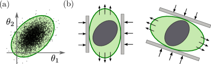
Figure 1: Schematic of error ellipse and its quantum-limited hard core. (a) Error ellipse represents the concentration characteristics of estimates in parameter space. (b) Measurement incompatibility forbids the error ellipse (filled with green) to stick close to the quantum-limited ellipse (filled with black) simultaneously in all directions.

Optimization of estimation precision means shrinking the error ellipsoid as small as possible. The CCRB $n\mathcal{E}\geq F^{-1}$ implies that the error ellipsoid must wholly contain the ellipsoid defined by $(v-\theta)^{\mkern-1.5mu\mathsf{T}}F(v-\theta)=\kappa^{2}$ [31, 32], which we call the classical-limited ellipsoid for a given measurement henceforth. Due to the asymptotic attainability of the CCRB [30, 31, 33], the smallest error ellipsoid in the asymptotic regime is exactly the classical-limited ellipsoid. On the other hand, the Braunstein-Caves inequality [4] $F\leq\mathcal{F}$ implies that the classical-limited ellipsoid in turn must entirely contain the quantum-limited one given by $(v-\theta)^{\mkern-1.5mu\mathsf{T}}\mathcal{F}(v-\theta)=\kappa^{2}$ [2]. However, the error ellipsoid cannot stick close to the quantum-limited core simultaneously in all directions through the optimization of quantum measurements if the measurement incompatibility is present, as illustrated in Fig. 1(b). How to quantitatively describe the mechanism behind it is the crucial task of quantum multiparameter estimation theory and is exactly answered by the TEUR.

Parameter correlation.— We say the parameters in a quantum statistical model are correlated if the QFIM is not diagonal and say the estimates are correlated if the covariance matrix $\mathcal{E}$ is not diagonal. Now, we use the error ellipse approach to analyze the impact of parameter correlation on the IRTR. Without loss of generality, we move the mean $\bar{\theta}$ of estimates to the origin of parameter space and set $\kappa=1$. Assume that the error ellipse attains the CCRB, that is, $n\mathcal{E}=F^{-1}$. Then, the intersection of the error ellipse with the horizontal and vertical axes are given by $\ell_{1}=1/\sqrt{F_{11}}$ and $\ell_{2}=1/\sqrt{F_{22}}$, as shown in Fig. 2(a). The IRTR impose a tradeoff between the diagonal elements of the CFIM and thereby restricts simultaneous reduction of $\ell_{1}$ and $\ell_{2}$. However, the IRTR does not account for the parameter correlation, as it is irrelevant to the off-diagonal elements of the CFIM and the QFIM. As a result, the IRTR does not give the full information about what kinds of error ellipses can be achieved by quantum multiparameter estimation strategies. For instance, the red dashed ellipse in Fig. 2(b) has the intersections that satisfy the IRTR but cannot be realized by any quantum estimation strategy, because it breaks the quantum-limited ellipse.

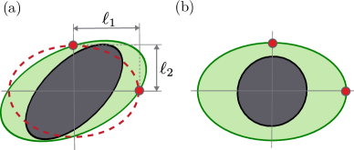
Figure 2: Error ellipse and its quantum limits. (a) For a general estimation problem, the error ellipse and the quantum-limited ellipse may be tilted due to parameter correlation. (b) Under a suitable reparametrization, the quantum-limited ellipse becomes a circle, while the error ellipse is rendered erect.

The reparametrization approach employed in the proof of the TEUR ensures that the IRTR is always applied to an appropriately transformed parameter space, where the quantum-limited ellipse become a circle and the error ellipse aligned with the axes, as illustrated in Fig. 2(b). In such a framework, all information about parameter correlation is encapsulated in the reparametrization process and can subsequently be incorporates into the tradeoff relation by reverting to the original parameters. Consequently, the TEUR simultaneously account for both measurement incompatibility and parameter correlation in quantum multiparameter estimation.

Example.— We here use the TEUR to study the estimation of the phase-space displacement of a bosonic mode, whose annihilation operator and creation operator are denoted by $a$ and $a^{\dagger}$, respectively. Assume that the bosonic mode is initially in a squeezed vacuum state $S(\zeta)\ket{0}$, where $\ket{0}$ denotes the vacuum state and $S(\zeta)=\operatorname{exp}(\zeta^{*}a^{2}/2-\zeta a^{\dagger 2}/2)$ with $\zeta=r\exp(i\varphi)$ being the squeeze parameter is the squeeze operator. The state before measurement is a displaced squeezed state $\ket{\alpha;\zeta}=D(\alpha)S(\zeta)\ket{0}$, where $D(\alpha)=\exp(\alpha a^{\dagger}-\alpha^{*}a)$ with $\alpha\in\mathbb{C}$ is the displacement operator. The parameters of interest here are the real and imaginary parts of $\alpha$, that is, $\theta_{1}=\real\alpha$ and $\theta_{2}=\imaginary\alpha$. We obtain the quantum geometric tensor [48]:

where

The TEUR is given by $|n\mathcal{E}\mathcal{F}-I|\geq 1$ as $\gamma=1$.

To construct a class of measurements that saturate the TEUR, we first prepare an ancillary bosonic mode and then measure a pair of commuting observables $\mathcal{A}=Q-Q^{\prime}$ and $\mathcal{B}=P+P^{\prime}$, where $Q=(a+a^{\dagger})/2$ and $P=(a-a^{\dagger})/(2i)$ are the quadrature operators for the system and $Q^{\prime}$ and $P^{\prime}$ are the quadrature operators for the ancillary mode, as illustrated in Fig. 3(a). We take the sample means [50] of outcomes of measuring $\mathcal{A}$ and $\mathcal{B}$ as the estimate of $\theta_{1}$ and $\theta_{2}$, respectively. The estimators are unbiased when the initial state of the ancillary mode satisfy $\expectationvalue{Q^{\prime}}=\expectationvalue{P^{\prime}}=0$. As the system and the ancilla are initially uncorrelated, the covariance matrix of estimators is given by

$$n\mathcal{E}=V(Q,P)+V(-Q^{\prime},P^{\prime}),$$ (9)

where $V(X_{1},X_{2})_{\mu\nu}=\real\expectationvalue{X_{\mu}X_{\nu}}-\expectationvalue{X_{\mu}}\expectationvalue{X_{\nu}}$ is defined for any two Hermitian operators $X_{1}$ and $X_{2}$. After some algebra, we obtain [48]

$$V(Q,P)=\frac{1}{4}R\quantity(\frac{\varphi}{2})C(-2r)R\quantity(\frac{\varphi}{2})^{\mkern-1.5mu\mathsf{T}},$$ (10)

which equals the QCRB, so the second term of Eq. (9) is the extra error covariance due to measurement incompatibility. As a result, the TEUR is equivalent to $|V(-Q^{\prime},P^{\prime})|\geq 1/16$ and thus can be saturated when the ancillary mode is in a minimum uncertainty state.

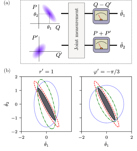
Figure 3: Phase-space displacement estimation. (a) Protocol of the joint measurements implemented with an ancillary mode, which is prepared in a squeezed vacuum state with the squeeze parameter $r^{\prime}e^{i\varphi^{\prime}}$. (b) Error ellipses and quantum-limited ellipse (filled with black) for the joint estimation. Here, the system state is a displaced squeezed state with $r=1$ and $\varphi=\pi/3$. In the left panel, the measurements are given by $\varphi^{\prime}=-\pi/3$ (red dashed), $\varphi^{\prime}=0$ (green dash-dotted) and $\varphi^{\prime}=\pi/3$ (blue dotted), where $r^{\prime}$ is set to $1$. In the right panel, the measurements are given by $r^{\prime}=1$ (red dashed), $r^{\prime}=0$ (green dash-dotted) and $r^{\prime}=-1$ (blue dotted), where $\varphi^{\prime}$ is set to $-\pi/3$. The shapes of the error ellipses and the quantum-limited ellipses are independent of the true values of $\theta_{1}$ and $\theta_{2}$, which are set to zero for convenience.

Preparing the ancillary mode in a squeezed vacuum state with a squeeze parameter $\zeta^{\prime}=r^{\prime}e^{i\varphi^{\prime}}$, the extra error covariance becomes

$$V(-Q^{\prime},P^{\prime})=\frac{1}{4}R\quantity(-\frac{\varphi^{\prime}}{2})C(-2r^{\prime})R\quantity(-\frac{\varphi^{\prime}}{2})^{\mkern-1.5mu\mathsf{T}}.$$ (11)

All the resultant covariance matrices saturate the TEUR, no matter what the values of $r^{\prime}$ and $\varphi^{\prime}$ are. When $\varphi^{\prime}=-\varphi$, the principal axes of the error ellipses are aligned with that of the quantum-limited ellipse, as shown in the left panel of Fig. 3(b). The right panel of Fig. 3(b) shows that, by changing $r^{\prime}$, we can reduce the estimation error in one direction at the cost of increasing the estimation error in the other direction. This cost will be tremendous if the error ellipse gets close to the quantum-limited core in any direction.

No strict inclusion relationship exists between the error ellipses of joint estimation strategies that achieve TEUR saturation. Therefore, the performance comparability in terms the Loewner partial order [51] of covariance matrices is no longer applicable. For such a case, the quantity $|n\mathcal{E}|^{1/2}$, which corresponds to the estimator volume [52], provides a useful metric for assessing the relative performance of different joint estimation strategies. Using the Minkowski determinant inequality, we get the lower bound of the area of the error ellipses:

$$|n\mathcal{E}|^{1/2}\geq|V(Q,P)|^{1/2}+|V(-Q^{\prime},P)|^{1/2}=1/2.$$ (12)

Its minimum can be attained by $r=r^{\prime}$ and $\varphi^{\prime}=-\varphi$.

Conclusion.— To summarize, we have derived an estimation uncertainty relation that captures the impact of measurement incompatibility and parameter correlation on quantum two-parameter estimation. It completely describes the quantum limit of two-parameter estimation precision with pure states. For cases of more than two parameters, it is promising to recast any multiparameter estimation problem into a series of two-parameter estimation problems through reparametrization. At least for pure states, such an approach can always be implemented, as the quantum geometric tensor thereof can be transformed by reparametrization into block-diagonal forms with each block being at most two-dimensional [53, 54].

We have developed the error-ellipse approach to visualizing the impact of measurement incompatibility on the estimation precision with parameter correlation, where the variances of estimates alone are insufficient to characterize the estimation precision. The error ellipse is widely used in quantum optics to represent the fluctuations distribution of amplitude operators in phase space, particularly for illustrating the properties of squeezed states [55, 56]. In such contexts, the error ellipse corresponds to the quantum-limited ellipse in our phase-space complex displacement estimation example. However, it does not represent the actual error ellipse of the estimates in practical scenarios. With the TEUR, we have treated the actual error ellipse of multiparameter estimation and the error ellipse in phase space for quantum optics in a unified framework.

Last, the TEUR would also be helpful to find the optimal measurement for single-parameter estimation. Single parameter estimation can be embedded into a two-parameter one by introducing an auxiliary parameter, e.g., the phase-space real displacement estimation problem can be dilated to the joint estimation of the complex displacement. When the auxiliary parameter is orthogonal to the original one and the incompatibility factor $\gamma$ is unit, the TEUR Eq. (3) leads us to a crucial clue about optimal measurement for the original single-parameter estimation problem, that is, the optimal measurement must extract no distinguishability about the auxiliary parameter. How to appropriately embed single-parameter estimation into a two-parameter one and construct the optimal measurement will be explored in future work.

Supplementary Materials

Appendix S-1 Derivation of the two-parameter estimation uncertainty relation

We here give the detailed derivation of two-parameter estimation uncertainty relation (TEUR). We use the information regret tradeoff relation (IRTR) [24] as the starting point. Let $F$ and $\mathcal{F}$ denote the classical Fisher information matrix (CFIM) and the quantum Fisher information matrix (QFIM), respectively. The inefficiency of a quantum measurement for estimating the $\mu$-th parameter $\theta_{\mu}$ can be quantified by the regret ratio defined by [24]

$$\Delta_{\mu}\equiv\sqrt{\frac{\mathcal{F}_{\mu\mu}-F_{\mu\mu}}{\mathcal{F}_{\mu\mu}}}.$$ (S1)

The IRTR for any quantum measurement is given by

$$\Delta_{\mu}^{2}+\Delta_{\nu}^{2}+2\sqrt{1-c_{\mu\nu}^{2}}\Delta_{\mu}\Delta_{\nu}\geq c_{\mu\nu}^{2}\mbox{\quad with\quad}c_{\mu\nu}\equiv\frac{\norm{\sqrt{\rho}[L_{\mu},L_{\nu}]\sqrt{\rho}}_{1}}{2\sqrt{\mathcal{F}_{\mu\mu}\mathcal{F}_{kk}}},$$ (S2)

where $\norm{X}_{1}\equiv\tr\sqrt{X^{\dagger}X}$ denotes the Schatten-1 norm of an operator $X$, $L_{\mu}$ is the symmetric logarithmic derivative (SLD) operator about $\theta_{\mu}$, and $\rho$ is the density operator of the system.

Notice that the IRTR only involves the diagonal elements of the CFIM and thus gives no constraint on the off-diagonal elements of the CFIM. We include the off-diagonal elements of the CFIM in the IRTR by utilizing parameter transformations in what follows. Let $\phi=(\phi_{1},\phi_{2},\dots,\phi_{d})$ be a set of new parameters, which are functions of the original parameters $\theta=(\theta_{1},\theta_{2},\dots,\theta_{d})$. The CFIM and the QFIM about $\phi$ are give by [9]

$$\mathcal{F}^{\prime}=J^{\mkern-1.5mu\mathsf{T}}\mathcal{F}J\mbox{\quad and\quad}F^{\prime}=J^{\mkern-1.5mu\mathsf{T}}FJ,$$ (S3)

respectively, where $J_{\mu\nu}\equiv\partialderivative*{\theta_{\mu}}{\phi_{\nu}}$ are the elements of the Jacobian matrix. We here use the prime symbol ^′ to denote the quantities about the new parameters. Let us now choose a special kind of parameter transformation whose Jacobian matrix is of the form $\mathcal{F}^{-1/2}O$, where $O$ is an arbitrary orthogonal matrix. In such case, according to Eq. (S3), the QFIM about $\phi$ becomes the identity matrix no matter what the orthogonal matrix $O$ is. Meanwhile, the CFIM about $\phi$ is given by

$$F^{\prime}=O^{\mkern-1.5mu\mathsf{T}}\mathcal{F}^{-1/2}F\mathcal{F}^{-1/2}O.$$ (S4)

Furthermore, we can always find an orthogonal matrix $O$ to diagonalize the CFIM and call such parameters $\phi$ the canonical parameters. The regret ratio about the canonical parameter $\phi_{\mu}$ is $\Delta^{\prime}_{\mu}=\sqrt{1-F^{\prime}_{\mu\mu}}$ as $\mathcal{F}_{\mu\nu}=\delta_{\mu\nu}$. Consequently, the IRTR about two canonical parameters is given by

$$2-F^{\prime}_{\mu\mu}-F^{\prime}_{\nu\nu}+2\sqrt{\quantity[1-(c^{\prime}_{\mu\nu})^{2}](1-F^{\prime}_{\mu\mu})(1-F^{\prime}_{\nu\nu})}\geq(c^{\prime}_{\mu\nu})^{2},$$ (S5)

where $c^{\prime}_{\mu\nu}=\frac{1}{2}\norm{\sqrt{\rho}[L^{\prime}_{\mu},L^{\prime}_{\nu}]\sqrt{\rho}}_{1}$ with $L^{\prime}_{\mu}$ being the SLD operator about $\phi_{\mu}$. For two-parameter estimation problem, the IRTR about canonical parameters can be expressed as

$$2-\tr(F^{\prime})+2\sqrt{\quantity[1-(c^{\prime}_{12})^{2}]\quantity[1-\tr(F^{\prime})+|F^{\prime}|]}\geq(c^{\prime}_{12})^{2},$$ (S6)

where we have used $F^{\prime}_{11}F^{\prime}_{22}=|F^{\prime}|$ as the CFIM about the canonical parameters is diagonal.

We now transform the inequality Eq. (S6) from the canonical parameters to the original ones. To do so, we express $c^{\prime}_{\mu\nu}$ with the quantities about the original parameters. The SLD operators about $\phi_{\nu}$ can be expressed as

$$L^{\prime}_{\nu}=\sum_{\mu}J_{\mu\nu}L_{\mu},$$ (S7)

which can be seen from $\partialderivative*{\phi_{\nu}}=\sum_{\mu}J_{\mu\nu}\partialderivative*{\theta_{\mu}}$ and $\partialderivative*{\rho}{\phi_{\nu}}=(L^{\prime}_{\nu}\rho+\rho L^{\prime}_{\nu})/2$. It follows from Eq. (S7) that

$$[L^{\prime}_{1},L^{\prime}_{2}] =[J_{11}L_{1}+J_{21}L_{2},J_{12}L_{1}+J_{22}L_{2}]$$

$$=(J_{11}J_{22}-J_{21}J_{12})[L_{1},L_{2}]$$

$$=|J|\,[L_{1},L_{2}]$$

$$=|\mathcal{F}|^{-1/2}[L_{1},L_{2}],$$ (S8)

where we have used $|J|=|\mathcal{F}^{-1/2}O|=|\mathcal{F}|^{-1/2}$ in the last equality. Therefore, we get

$$c^{\prime}_{12} =\frac{1}{2}\norm{\sqrt{\rho}[L^{\prime}_{1},L^{\prime}_{2}]\sqrt{\rho}}_{1}=\frac{1}{2}\norm{\sqrt{\rho}[L_{1},L_{2}]\sqrt{\rho}}_{1}\,|\mathcal{F}|^{-1/2}.$$ (S9)

Meanwhile, it follows from Eq. (S4) that

$$\tr(F^{\prime})=\tr(F\mathcal{F}^{-1})\mbox{\quad and\quad}|F^{\prime}|=|F\mathcal{F}^{-1}|.$$ (S10)

Substituting Eqs. (S9) and (S10) into Eq. (S6), we get

$$\tr(F\mathcal{F}^{-1})-2\sqrt{(1-\gamma)\quantity[1-\tr(F\mathcal{F}^{-1})+|F\mathcal{F}^{-1}|]}\leq 2-\gamma,$$ (S11)

where $\gamma$ is the incompatibility factor defined as

$$\gamma=\frac{\norm{\sqrt{\rho}[L_{1},L_{2}]\sqrt{\rho}}_{1}^{2}}{4\,|\mathcal{F}|}.$$ (S12)

We now show how to rewrite Eq. (S11) regarding to the error-covariance matrix $\mathcal{E}$. For any two-dimensional matrix $G$, it is easy to verify that

$$\tr(G)=1+|G|-|I-G|.$$ (S13)

Taking $G=F\mathcal{F}^{-1}$, it follows that

$$\tr(F\mathcal{F}^{-1})=1+|F\mathcal{F}^{-1}|-|I-F\mathcal{F}^{-1}|.$$ (S14)

Substituting the above expression into Eq. (S11) and multiplying both sides by $|F^{-1}|$, we get

$$|F^{-1}|+|\mathcal{F}^{-1}|-|F^{-1}-\mathcal{F}^{-1}|-2\sqrt{(1-\gamma)|F^{-1}|\times|F^{-1}-\mathcal{F}^{-1}|}\leq(2-\gamma)|F^{-1}|,$$ (S15)

which can be simplified into

$$(1-\gamma)|F^{-1}|+|F^{-1}-\mathcal{F}^{-1}|+2\sqrt{(1-\gamma)|F^{-1}|\times|F^{-1}-\mathcal{F}^{-1}|}\geq|\mathcal{F}^{-1}|.$$ (S16)

Taking the square root of both sides of the above inequality, we get

$$\sqrt{(1-\gamma)|F^{-1}|}+\sqrt{|F^{-1}-\mathcal{F}^{-1}|}\geq\sqrt{\quantity|\mathcal{F}^{-1}|}.$$ (S17)

Notice that the CRB and QCRB imply that $|n\mathcal{E}|\geq|F^{-1}|$ and $|n\mathcal{E}-\mathcal{F}^{-1}|\geq|F^{-1}-\mathcal{F}^{-1}|$. Therefore, combining Eq. (S17) and the CRBs, we get

$$\sqrt{(1-\gamma)|n\mathcal{E}|}+\sqrt{|n\mathcal{E}-\mathcal{F}^{-1}|}\geq\sqrt{\quantity|\mathcal{F}^{-1}|}.$$ (S18)

Multiplying both sides of the above inequality by $\sqrt{|\mathcal{F}|}$, we get

$$\sqrt{\quantity(1-\gamma)|n\mathcal{E}\mathcal{F}|}+\sqrt{|n\mathcal{E}\mathcal{F}-I|}\geq 1,$$ (S19)

which is the TEUR presented in the main text.

Appendix S-2 Brief review on the geometry of ellipse

Let us consider an ellipse constituted by the coordinates $v=(x,y)^{\mkern-1.5mu\mathsf{T}}$ that satisfy $v^{\mkern-1.5mu\mathsf{T}}A\ v=1$, where $A$ is a real symmetric and positive two-dimensional matrix. With the elements of $A$ denoted by $A_{jk}$, the equation of the ellipse can be expressed as

$$A_{11}x^{2}+2A_{12}xy+A_{22}y^{2}=1$$ (S20)

The principal axes of the ellipse are given by the eigenvectors of $A$. The length of the semi-axes are given by $1/\sqrt{\lambda_{j}}$ for $j=1,2$, where $\lambda_{j}$ is the eigenvalues of $A$. Figure S1 illustrates the concepts of intercepts and maximum values of a tilted ellipse. The intercepts of the ellipse are given by

$$x_{\mathrm{int}}=1/\sqrt{A_{11}}\mbox{\quad and\quad}y_{\mathrm{int}}=1/\sqrt{A_{22}},$$ (S21)

which can be seen by setting $y=0$ or $x=0$ in the equation of ellipse, that is, Eq. (S20). The maximum values of the ellipse are given by

$$x_{\mathrm{max}}=\sqrt{(A^{-1})_{11}}\mbox{\quad and\quad}y_{\mathrm{max}}=\sqrt{(A^{-1})_{22}},$$ (S22)

which can be derived as follows. To obtain the maximum values, e.g., $y_{\mathrm{max}}$, we can express Eq. (S20) as

$$1 =A_{11}\quantity[x+(A_{11})^{-1}A_{12}\ y]^{2}+[A_{22}-(A_{11})^{-1}(A_{12})^{2}]\ y^{2}$$

$$=A_{11}\quantity[x+(A_{11})^{-1}A_{12}\ y]^{2}+(A_{11})^{-1}|A|\ y^{2},$$ (S23)

where the symbol $|A|$ denotes the determinant of the matrix $A$. It follows that

$$y^{2}\leq A_{11}/|A|,$$ (S24)

where the equality holds when $x=-(A_{11})^{-1}A_{12}y$. This means that

$$y_{\mathrm{max}}=\sqrt{A_{11}/|A|}.$$ (S25)

Using the formula

$$\matrixquantity(a&b\\ c&d)^{-1}=\frac{1}{ad-bc}\matrixquantity(d&-b\\ -c&a).$$ (S26)

for the inverse of a two-dimensional matrix, we get $y_{\mathrm{max}}=\sqrt{(A^{-1})_{22}}$. The value of $x_{\mathrm{max}}$ can be obtained in a similar way.

Substituting $A$ by $(n\mathcal{E})^{-1}$, we can get the intersections and the maximum values of the error ellipse. Substituting $A$ by $F$ and $\mathcal{E}$, we can get the intersections and the maximum values of the classical-limited ellipse and the quantum-limited ellipse, respectively.

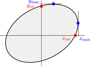
Supp. Fig. S1: The intercepts and the maximum values of a tilted ellipse.

Appendix S-3 Example: Estimating a complex signal with squeezed state

Let us consider the scenario of using a squeezed vacuum state as the initial state to estimate a complex parameter $\alpha$ of the displacement operator $D(\alpha):=\exp(\alpha a^{\dagger}-\alpha^{*}a)$ acting on the initial state. The quantum state to be measured is the displaced squeezed state

$$\ket{\alpha;\zeta}:=D(\alpha)S(\zeta)\ket{0},$$ (S27)

where $S(\zeta):=\exp(\frac{\zeta^{*}}{2}a^{2}-\frac{\zeta}{2}(a^{\dagger})^{2})$ is the squeeze operator with $\zeta:=r\exp(i\varphi)$ being the squeeze parameter and $\ket{0}$ is the vacuum state. The parameters of interest here are the real and imaginary parts of $\alpha$, i.e., $\theta_{1}=\real\alpha$ and $\theta_{2}=\imaginary\alpha$.

To apply the TEUR, we need to calculate the QFIM and the incompatibility factor; Both of them can be determined by the quantum geometric tensor [46]:

$$\mathcal{Q}_{jk}=\quantity(\partialderivative{\bra{\alpha;\zeta}}{\theta_{j}})\quantity(\mathbbm{1}-\outerproduct{\alpha;\zeta}{\alpha;\zeta})\quantity(\partialderivative{\ket{\alpha;\zeta}}{\theta_{k}}),$$ (S28)

where $\mathbbm{1}$ denotes the identity operator. The QFIM and the incompatibility factor for pure states are given by

$$\mathcal{F}=4\real\mathcal{Q}\mbox{\quad and\quad}\gamma=\frac{(\imaginary\mathcal{Q}_{12})^{2}}{|\real\mathcal{Q}|},$$ (S29)

respectively. Instead of straightforwardly calculating $\mathcal{F}$ and $\gamma$ from definitions, we here utilize the following relation between the displaced squeezed state and the squeezed coherent state [57, see Sec. 5.1]:

$$D(\alpha)S(\zeta)\ket{0}=S(\zeta)D(\beta)\ket{0}\mbox{\quad with\quad}\beta=\alpha\cosh r+\alpha^{*}e^{i\varphi}\sinh r.$$ (S30)

Because $S(\zeta)$ is a unitary operator independent of the parameters to be estimated, the quantum geometric tensor for the parametric states $\ket{\alpha;\zeta}$ equals that for the coherent state $D(\beta)\ket{0}$. The quantum geometric tensor of $D(\beta)\ket{0}$ with respect to the parameters $\tilde{\theta}_{1}:=\real\beta$ and $\tilde{\theta}_{2}=\imaginary\beta$ is known as [24]

$$\tilde{\mathcal{Q}}=\matrixquantity(1&i\\ -i&1).$$ (S31)

The quantum geometric tensor regarding to $\theta_{1}$ and $\theta_{2}$ can be obtained from $\mathcal{Q}=J^{\mkern-1.5mu\mathsf{T}}\tilde{\mathcal{Q}}J$, where $J$ is the Jacobian matrix defined as $J_{\mu\nu}=\partial\tilde{\theta}_{\mu}/\partial\theta_{\nu}$. It follows from Eq. (S30) that

$$J=\matrixquantity(\cosh r+\cos\varphi\sinh r&\sin\varphi\sinh r\\ \sin\varphi\sinh r&\cosh r-\cos\varphi\sinh r),$$ (S32)

which can be decomposed into the combination of two rotation matrices and a scaling matrix, that is,

$$J=R\quantity(\frac{\varphi}{2})C(r)R\quantity(\frac{\varphi}{2})^{\mkern-1.5mu\mathsf{T}}\mbox{\quad with\quad}R(\varphi)=\matrixquantity(\cos\varphi&-\sin\varphi\\ \sin\varphi&\cos\varphi)\mbox{\quad and\quad}C(r)=\matrixquantity(e^{r}&0\\ 0&e^{-r}).$$ (S33)

We thus obtain the quantum geometric tensor with respect to the parameters $\theta_{1}$ and $\theta_{2}$:

which implies

$$\mathcal{F}=4\,R\quantity(\frac{\varphi}{2})C(2r)R\quantity(\frac{\varphi}{2})^{\mkern-1.5mu\mathsf{T}}=4\matrixquantity(\cosh 2r+\cos\varphi\sinh 2r&\sin\varphi\sinh 2r\\ \sin\varphi\sinh 2r&\cosh 2r-\cos\varphi\sinh 2r)\mbox{\quad and\quad}\gamma=1.$$ (S34)

Accordingly, the TEUR becomes

$$|\mathcal{E}\mathcal{F}-I|\geq 1.$$ (S35)

The quantum measurements that attain the TEUR can be constructed as follows. Let us consider an ancillary mode whose annihilation operator are denote by $a^{\prime}$. Define the Hermitian operators for these two modes as

$$Q =\frac{a+a^{\dagger}}{2},\quad P=\frac{a-a^{\dagger}}{2i},$$ (S36)

$$Q^{\prime} =\frac{a^{\prime}+a^{\prime\dagger}}{2},\quad P^{\prime}=\frac{a^{\prime}-a^{\prime\dagger}}{2i}.$$ (S37)

Let us consider the following two observable

$$\mathcal{A}=Q-Q^{\prime}\mbox{\quad and\quad}\mathcal{B}=P+P^{\prime},$$ (S38)

which can be jointly measured as $[\mathcal{A},\mathcal{B}]=0$. We take the sample mean of the outcomes of $\mathcal{A}$ and $\mathcal{B}$ as the estimates for $\theta_{1}$ and $\theta_{2}$, respectively. The unbiasedness condition requires that

$$\expectationvalue{\mathcal{A}}=\real\alpha\mbox{\quad and\quad}\expectationvalue{\mathcal{B}}=\imaginary\alpha,$$ (S39)

where the expectation is taken with respect to the quantum state $\ket{\alpha;\zeta}\otimes\ket{\mathrm{anc}}$ with $\ket{\mathrm{anc}}$ denoting the initial state of the ancillary mode. The unbiasedness condition Eq. (S39) implies that $\expectationvalue{Q^{\prime}}{\mathrm{anc}}=\expectationvalue{P^{\prime}}{\mathrm{anc}}=0$. The error-covariance matrix for the above estimators is then given by $\mathcal{E}=n^{-1}V(\mathcal{A},\mathcal{B})$, where we define the covariance matrix of operators $X_{\mu}$ as

$$[V(X_{1},X_{2})]_{\mu\nu}=\real\expectationvalue{X_{\mu}X_{\nu}}-\expectationvalue{X_{\mu}}\expectationvalue{X_{\nu}}.$$ (S40)

Since the system and the ancilla are initially uncorrelated, we have

$$V(\mathcal{A},\mathcal{B})=V(Q,P)+V(-Q^{\prime},P^{\prime}).$$ (S41)

The state of the sensing system before measurement is the displaced squeezed state $D(\alpha)S(\zeta)\ket{0}$. The quantum expectation of an arbitrary operator $X$ in the displaced squeezed state is equal to the quantum expectation of $\widetilde{X}=S(\zeta)^{\dagger}D(\alpha)^{\dagger}XD(\alpha)S(\zeta)$ in the vacuum state. It follows from

$$D(\alpha)^{\dagger}aD(\alpha)=a+\alpha\mbox{\quad and\quad}S(\zeta)^{\dagger}ae^{-i\varphi/2}S(\zeta)=ae^{-i\varphi/2}\cosh r-a^{\dagger}e^{i\varphi/2}\sinh r$$ (S42)

that

The quadrature operators in the Heisenberg picture can be expressed as

$$\matrixquantity(\widetilde{Q}\\ \widetilde{P})=K\matrixquantity(\widetilde{a}\\ \widetilde{a^{\dagger}})\mbox{\quad with\quad}K=\frac{1}{2}\matrixquantity(1&1\\ -i&i).$$ (S43)

It then follows that

(S44)

Using $\expectationvalue{Q^{2}}{0}=\expectationvalue{P^{2}}{0}=1/4$ and $\real\!\expectationvalue{QP}{0}=\expectationvalue{Q}{0}=\expectationvalue{P}{0})=0$, we get

$$V(Q,P) =R\quantity(\frac{\varphi}{2})C(-r)R\quantity(\frac{\varphi}{2})^{\mkern-1.5mu\mathsf{T}}\matrixquantity(\frac{1}{4}{\frac{1}{4}})R\quantity(\frac{\varphi}{2})C(-r)R\quantity(\frac{\varphi}{2})^{\mkern-1.5mu\mathsf{T}}$$

$$=\frac{1}{4}R\quantity(\frac{\varphi}{2})C(-2r)R\quantity(\frac{\varphi}{2})^{\mkern-1.5mu\mathsf{T}}.$$ (S45)

Comparing Eq. (S34) and Eq. (S-3), it can be seen that $V(Q,P)=\mathcal{F}^{-1}$. Therefore, the TEUR is equivalent to

$$|V(-Q^{\prime},P^{\prime})|\geq|\mathcal{F}^{-1}|=\frac{1}{16}.$$ (S46)

This means that the TEUR can be saturated if we prepare the ancillary mode in squeezed vacuum state.

Assume that the ancillary mode is prepared in a squeezed vacuum state $\ket{\zeta^{\prime}}$ with the squeeze parameter $\zeta^{\prime}=r^{\prime}e^{i\varphi^{\prime}}$. It can be shown that the covariance matrix of the ancillary mode is given by

$$V(-Q^{\prime},P^{\prime})=\frac{1}{4}R\quantity(-\frac{\varphi^{\prime}}{2})C(-2r^{\prime})R\quantity(-\frac{\varphi^{\prime}}{2})^{\mkern-1.5mu\mathsf{T}}.$$ (S47)

If we consider $|V(\mathcal{A},\mathcal{B})|$ as a criterion, we have

$$|V(\mathcal{A},\mathcal{B})|^{1/2} =|V(Q,P)+V(-Q^{\prime},P^{\prime})|^{1/2}$$ (S48)

$$\geq|V(Q,P)|^{1/2}+|V(-Q^{\prime},P^{\prime})|^{1/2}$$ (S49)

$$=\frac{1}{4}|C(-2r)|^{1/2}+\frac{1}{4}|C(-2r^{\prime})|^{1/2}$$ (S50)

$$=\frac{1}{2},$$ (S51)

where the inequality follows from the Minkowski determinant inequality. This bound can be saturated when $\varphi^{\prime}=-\varphi$ and $r^{\prime}=r$.