Bulk Spacetime Encoding via Boundary Ambiguities

Abstract

We propose a method to reconstruct the exterior of a static, planar-symmetric black hole from an infinite set of discrete momentum-space locations, known as pole-skipping points, where the boundary Green’s function becomes ambiguous. The reconstruction is fully analytical and involves solving only linear equations. It further enables a reinterpretation of any pure gravitational field equation in pole-skipping data. Moreover, our method reveals that the pole-skipping points are redundant: only a subset is independent, while the rest are fixed by an equal number of homogeneous polynomial constraints. These identities are universal, independent of the details of the bulk geometry, including its dimensionality, asymptotic behavior, or the existence of a holographic duality.

Introduction—The holographic duality, exemplified by the Anti-de Sitter/Conformal Field Theory (AdS/CFT) correspondence, stands as a profound bridge linking quantum gravity in asymptotically AdS spacetimes to strongly coupled CFTs living on their boundaries [1, 2, 3]. Despite its wide-ranging applications across areas such as condensed matter physics, quantum chromodynamics, and quantum information theory [4, 5, 6, 7, 8], a complete understanding of how the bulk spacetime emerges from boundary CFT remains elusive. This fundamental problem hinders efforts to extend holographic duality to more general quantum field theories and realistic systems, including strange metals and our very universe.

Numerous studies have explored bulk spacetime reconstruction, such as [9, 10, 11, 12, 13, 14, 15, 16, 17, 18, 19, 20, 21, 22, 23], many of which are inspired by the perspective that spacetime is built up with quantum entanglement [24, 25, 26, 27, 28]. In this Letter, we present a different line of reasoning: the bulk spacetime can be explicitly encoded through special boundary locations, known as “pole-skipping points”, where the Green’s function becomes ambiguous.

Pole-skipping points are a universal feature of holographic Green’s functions, appearing at complex Matsubara frequencies and specific momenta where poles and zeros intersect, rendering the Green’s function ambiguous, or in other words, non-uniquely defined. This phenomenon was first discovered in the energy density retarded Green’s function, where the pole-skipping point lies in the upper-half complex frequency plane and encodes distinct signatures of quantum chaos [29, 30, 31]. It has since been connected to a certain horizon symmetry [32] and interpreted in terms of a gravitational replica manifold that captures the late-time entanglement wedge [33]. Beyond quantum chaos, an infinite tower of pole-skipping points has also been found in the lower-half complex frequency plane in other classes of Green’s functions [34].

From the bulk gravity perspective, pole-skipping points can be identified either through a near-horizon analysis [31, 34] or via the covariant expansion formalism [35, 36], both applied to the near-horizon bulk equations of motion. To date, pole-skipping has been observed in a wide variety of contexts [37, 38, 39, 40, 41, 34, 42, 43, 44, 45, 46, 47, 48, 49, 50, 51, 52, 53], including higher-derivative gravity theories [38, 40, 41] and purely field-theoretic models [37, 44, 45].

More recently, Ref. [54] argued that the infinite pole-skipping points lying along a single hydrodynamic mode, expanded in large spacetime dimensions, suffice to reconstruct the quasinormal spectrum and related Green’s function. This suggests that holographic Green’s functions can be efficiently encoded with reduced information, with pole-skipping points serving as carriers of key information.

In this Letter, we demonstrate that an infinite set of lower-half pole-skipping points can reconstruct the metric of a general static, planar-symmetric black hole geometry in arbitrary dimension. Provided the geometry uniquely determines the Green’s function, it immediately implies that the latter can be recovered from these pole-skipping points, for any spacetime dimension. This validates the results in [54], albeit via a different route.

Remarkably, our reconstruction is fully analytical and requires only elementary arithmetic—namely, solving linear equations. This explicit approach extends naturally to the vacuum Einstein equation, with any higher curvature correction, allowing a reinterpretation solely in boundary pole-skipping data.

Additionally, our reconstruction reveals that most pole-skipping points, as boundary input, are redundant and correspond to an equal number of homogeneous polynomial identities in the pole-skipping momenta. This indicates that the boundary field theory encodes the bulk spacetime redundantly, reminiscent of the holographic quantum error-correcting codes [55]. This Letter summarizes our companion paper [56].

Near-horizon analysis—To illustrate our reconstruction method, we begin by reviewing how pole-skipping points are determined via near-horizon analysis [34].

Consider a static, planar-symmetric black hole in $d+2$ dimensions. In ingoing Eddington–Finkelstein coordinates, the metric takes the form

$$ds^{2}=-g_{vv}(r)dv^{2}+g_{vr}(r)dvdr+r^{2}d\vec{x}^{2},$$ (1)

where $\vec{x}$ spans the $d$-dimensional spatial directions. In a holographic context, a thermal CFT with temperature $T_{b}$ exists at the boundary $r\to\infty$.

Now, take a massless probe scalar field $\phi$ coupled to the background, which satisfies the Klein-Gordon (KG) equation $\nabla^{2}\phi=0$. This scalar field is dual to a boundary marginal operator $\mathcal{O}$ with scaling dimension $\Delta=d+1$. After performing a Fourier transform $\phi=\varphi(r)e^{-i\omega v+i\vec{k}\vec{x}}$, the KG equation becomes

$$\frac{g_{vv}(r)}{g_{vr}(r)^{2}}\varphi^{\prime\prime}(r)+\left(-\frac{2i\omega}{g_{vr}(r)}+\frac{dg_{vv}(r)}{rg_{vr}(r)^{2}}-\frac{g_{vv}(r)g_{vr}^{\prime}(r)}{g_{vr}(r)^{3}}+\frac{g_{vv}^{\prime}(r)}{g_{vr}(r)^{2}}\right)\varphi^{\prime}(r)-\left(\frac{\mu}{r^{2}}+\frac{id\omega}{rg_{vr}(r)}\right)\varphi(r)=0,$$ (2)

where we have defined $\mu=k^{2}$. Without loss of generality, we set $r_{h}=1$ in the following. The metric components admit the near-horizon expansions:

$$g_{vv}(r)=g_{vv_{1}}(r-1)+g_{vv_{2}}(r-1)^{2}+\ldots$$ (3)

$$g_{vr}(r)=g_{vr_{0}}+g_{vr_{1}}(r-1)+g_{vr_{2}}(r-1)^{2}+\ldots$$

In this setup, the Hawking temperature is given by $T_{h}=\frac{g_{vv_{1}}}{4\pi g_{vr_{0}}}$. Meanwhile, the field $\varphi(r)$ admits a near-horizon expansion of the form

$$\varphi(r)=(r-1)^{\alpha}\sum_{p=0}^{\infty}\varphi_{p}(r-1)^{p},$$ (4)

with two exponents: $\alpha_{1}=0$ and $\alpha_{2}=\frac{i\omega}{2\pi T_{h}}$. Typically, for general $\omega$, only the $\alpha_{1}=0$ solution is ingoing at the horizon. Under this condition, the boundary retarded Green’s function of $\mathcal{O}$, denoted $\mathcal{G}^{\mathcal{O}}_{R}(\omega,\mu)$, can be uniquely determined as the ratio of the normalizable to the non-normalizable mode. However, at specific frequencies $\omega_{n}=-i2\pi nT_{h}$ for $n\in\mathbb{Z}^{+}$ and certain values of $\mu_{n}$, both modes become regular at the horizon, rendering ambiguous $\mathcal{G}^{\mathcal{O}}_{R}(\omega_{n},\mu_{n})$.

These special points are identified through performing near-horizon analysis. To begin with, we expand $\varphi(r)$, $g_{vv}(r)$ and $g_{vr}(r)$ around the horizon up to $n^{th}$ order and substitute them into the KG equation (2). By requiring the coefficients of $(r-1)^{n-1}$ to vanish for $n\geq 1$, we derive:

$$\mathbb{M}\cdot\varphi=\begin{pmatrix}M_{11}&2(2\pi T_{h}-i\omega)&0&\cdots&0\\ M_{21}&M_{22}&4(4\pi T_{h}-i\omega)&\cdots&0\\ \vdots&\vdots&\vdots&\ddots&\vdots\\ M_{n1}&M_{n2}&M_{n3}&\cdots&2n(2n\pi T_{h}-i\omega)\end{pmatrix}\begin{pmatrix}\varphi_{0}\\ \varphi_{1}\\ \vdots\\ \varphi_{n}\end{pmatrix}=\begin{pmatrix}0\\ 0\\ \vdots\end{pmatrix}.$$ (5)

The components $M_{ij}$ depend algebraically on $g_{vv_{m}}$ and $g_{vr_{m-1}}$ from (1). Once they are specified, the values of $\omega_{n}$ can be obtained by vanishing the last column of $\mathbb{M}$, yielding $\omega_{n}=-i2n\pi T_{h}$, while $\mu_{n}$ can be determined by solving the determinant equation $\text{Det}(\mathcal{M}^{(n)}(\omega_{n},\mu))=0$, or more compactly, $\text{Det}(\mathcal{M}^{(n)}(\boldsymbol{\mu}))=0$, where $\mathcal{M}^{(n)}$ denotes the first $n\times n$ submatrix of $\mathbb{M}$. Under these conditions, $\mathbb{M}\cdot\varphi=0$ admits two independent parameters, $\varphi_{0}$ and $\varphi_{n}$, thus confirming two ingoing solutions. For the KG equation (2), the associated $\text{Det}(\mathcal{M}^{(n)}(\boldsymbol{\mu}))=0$ defines a degree-$n$ polynomial in $\mu$, which we can express explicitly as

$$V_{n,n}\mu^{n}+V_{n,n-1}\mu^{n-1}+\cdots+V_{n,1}\mu+V_{n,0}=0,$$ (6)

where each $V_{n,m}$ denotes the coefficient of the term $\mu^{m}$ in $\text{Det}(\mathcal{M}^{(n)}(\boldsymbol{\mu}))$. By the fundamental theorem of algebra, this degree-$n$ polynomial admits $n$ roots, denoted $\mu_{n,q}$ for $q=1,\ldots,n$. Owing to its $S_{n}$ symmetry, one can construct $n$ elementary symmetric polynomials $E_{n}(\mu^{m})$, where $m=1,\ldots,n$ indicates the degree [57]. For example, $E_{3}(\mu^{2})=\mu_{3,1}\mu_{3,2}+\mu_{3,2}\mu_{3,3}+\mu_{3,3}\mu_{3,1}$.

Flipping Near-Horizon Analysis—To proceed with the bulk reconstruction, We now invert the previous near-horizon analysis by interchanging the roles of metric expansion coefficients $(g_{vr_{n-1}},\mkern 6.0mug_{vv_{n}})$ and the pole-skipping points $(\omega_{n},\mkern 6.0mu\mu_{n,q})$ in $\text{Det}(\mathcal{M}^{(n)}(\boldsymbol{\mu}))=0$. By recognizing the latter as given input and the former as unknowns, we reinterpret the determinant equation $\text{Det}(\mathcal{M}^{(n)}(\boldsymbol{\mu}))=0$ as $\text{Det}(\vec{\mathcal{M}}^{(n)}(\textbf{g}))=0$, thereby obtaining a system of $n$ equations for $g_{vv_{n}}$ and $g_{vr_{n-1}}$, with each equation corresponding to a distinct choice of $\mu_{n,q}$.

However, rather than working with each root $\mu_{n,q}$ individually, we find it more natural and illuminating to exploit the $S_{n}$ symmetry and instead formulate $\text{Det}(\vec{\mathcal{M}}^{(n)}(\textbf{g}))=0$ in terms of $n$ elementary symmetric polynomials $E_{n}(\mu^{m})$. These polynomials can be related to $g_{vv_{i}}$ and $g_{vr_{i-1}}$ via the polynomial coefficients $V_{n,m}$ in Eq. (6). Specifically, by invoking Vieta’s formula, we obtain

$$E_{n}(\mu^{m})=\frac{v_{n,n-m}}{v_{n,n}},$$ (7)

where we define $v_{n,m}=(-1)^{n-m}V_{n,m}$ for convenience. Here, $E_{n}(\mu^{m})$ serve as known parameters extracted from the set of pole-skipping points, while the coefficients $v_{n,m}$ are generally algebraic functions of $g_{vr_{i-1}}$ and $g_{vv_{i}}$. Under this reformulation, the $q^{\text{th}}$ equation in $\text{Det}(\vec{\mathcal{M}}^{(n)}(\textbf{g}))=0$, denoted $\text{Det}(\mathcal{M}^{(n)}_{q}(\textbf{g}))=0$, corresponds to the identity $E_{n}(\mu^{q})-\frac{v_{n,n-q}}{v_{n,n}}=0$.

Bulk reconstruction—We can then determine $g_{vv_{n}}$ and $g_{vr_{n-1}}$ by directly solving $\text{Det}(\vec{\mathcal{M}}^{(n)}(\textbf{g}))=0$. For $n=1$, $\text{Det}(\vec{\mathcal{M}}^{(1)}(\textbf{g}))=0$, derived from the KG equation (2), provides one equation: $E_{1}(\mu)+\frac{dg_{vv_{1}}}{2g_{vr_{0}}^{2}}=0$. A second equation arises by equating the boundary temperature $T_{b}$, expressed in $\omega_{1}$ as $T_{b}=i\frac{\omega_{1}}{2\pi}$, with the Hawking temperature $T_{h}=\frac{g_{vv_{1}}}{4\pi g_{vr_{0}}}$, leading to $i\frac{\omega_{1}}{2\pi}=\frac{g_{vv_{1}}}{4\pi g_{vr_{0}}}$. Solving these two equations yields:

$$g_{vv_{1}}=\frac{2d\omega_{1}^{2}}{E_{1}(\mu)},\quad g_{vr_{0}}=-\frac{id\omega_{1}}{E_{1}(\mu)},$$ (8)

where both $g_{vv_{1}}$ and $g_{vr_{0}}$ are expressed entirely in terms of the pole-skipping data: $\omega_{1}$ and $E_{1}(\mu)$ (i.e., $\mu_{1,1}$).

We proceed by considering $n=2$. Upon substituting the solutions for $g_{vv_{1}}$ and $g_{vr_{0}}$ from Eq. (8) into $\text{Det}(\vec{\mathcal{M}}^{(2)}(\textbf{g}))=0$, we obtain expressions for $g_{vv_{2}}$ and $g_{vr_{1}}$:

$$g_{vv_{2}}=\frac{d^{2}\omega_{1}^{2}E_{2}(\mu^{2})}{4E_{1}(\mu)^{3}}+\frac{2d^{2}\omega_{1}^{2}}{E_{1}(\mu)}-\frac{d^{2}\omega_{1}^{2}E_{2}(\mu)}{E_{1}(\mu)^{2}}+\frac{3d\omega_{1}^{2}}{E_{1}(\mu)},$$ (9)

$$g_{vr_{1}}=\frac{id^{2}\omega_{1}E_{2}(\mu)}{2E_{1}(\mu)^{2}}-\frac{id^{2}\omega_{1}}{E_{1}(\mu)}-\frac{id^{2}\omega_{1}E_{2}(\mu^{2})}{4E_{1}(\mu)^{3}}-\frac{id\omega_{1}}{E_{1}(\mu)}.$$

For $n>2$, the system $\text{Det}(\vec{\mathcal{M}}^{(n)}(\textbf{g}))=0$ becomes overdetermined, consisting of $n$ equations but only two variables: $g_{vv_{n}}$ and $g_{vr_{n-1}}$. However, as proved in [56], upon incorporating all the solutions for $g_{vv_{m}}$ and $g_{vr_{m-1}}$ with $m<n$ into $\text{Det}(\vec{\mathcal{M}}^{(n)}(\textbf{g}))=0$, the first $n-2$ equations become independent of $g_{vv_{n}}$ and $g_{vr_{n-1}}$. The last two equations: $\text{Det}(\mathcal{M}^{(n)}_{n-1}(\textbf{g}))=0$ and $\text{Det}(\mathcal{M}^{(n)}_{n}(\textbf{g}))=0$, corresponding respectively to

$$E_{n}(\mu^{n-1})-\frac{v_{n,1}}{v_{n,n}}=0,\quad E_{n}(\mu^{n})-\frac{v_{n,0}}{v_{n,n}}=0,$$ (10)

are both linear in $g_{vv_{n}}$ and $g_{vr_{n-1}}$. Moreover, they are linearly independent, as each involves an elementary symmetric polynomial of a different degree. We thus conclude that for all $n\geq 2$, the pair of equations $\text{Det}(\mathcal{M}^{(n)}_{n-1}(\textbf{g}))=0$ and $\text{Det}(\mathcal{M}^{(n)}_{n}(\textbf{g}))=0$ uniquely determines $g_{vv_{n}}$ and $g_{vr_{n-1}}$, provided a solution exists. They are fully expressible in terms of the pole-skipping data: $\omega_{1}$, $E_{m}(\mu^{m-1})$, and $E_{m}(\mu^{m})$ for all $m\leq n$.

The explicit expressions for $g_{vv_{n}}$ and $g_{vr_{n-1}}$ with $n>2$ are too lengthy to include here. However, by assuming that neither $g_{vv}(r)$ nor $g_{vr}(r)$ encounters any singularity before reaching the boundary, determining $g_{vv_{n}}$ and $g_{vr_{n-1}}$ for arbitrarily large $n$ enables the complete reconstruction of the exterior of the black hole.

We emphasize that, in the background (1) with $d>2$ in Einstein gravity, the KG equation (2) also describes the linearized Einstein equations for massless tensor perturbation modes, classified by their transformation properties under the little group $\text{SO}(d-1)$. In this context, the proposed reconstruction method remains applicable beyond the probe limit. As detailed in [56], our method extends straightforwardly to the massive KG equation of the form $(\nabla^{2}+m^{2})\phi=0$. Moreover, it is also applicable to backgrounds with Lifshitz scaling and hyperscaling violation [58, 59].

Reinterpret Einstein equation—The analytical reconstruction of the bulk metric immediately implies that the corresponding pure gravitational field equations can be explicitly reformulated in terms of boundary pole-skipping data. The simplest and most important example is the vacuum Einstein equation with a negative cosmological constant:

$$E_{\mu\nu}\equiv R_{\mu\nu}-\frac{1}{2}g_{\mu\nu}R+\Lambda g_{\mu\nu}=0,$$ (11)

where $\Lambda=-\frac{d(d+1)}{2}$, with the AdS radius set to unity. Expanding near the horizon up to zeroth order yields three nontrivial components: $E_{vr_{0}}=0$, $E_{rr_{0}}=0$, and $E_{xx_{0}}=0$. Upon substituting the reconstructed metric components from Eqs. (8) and (9), these equations can be rewritten entirely in terms of pole-skipping data:

$$E_{vr_{0}}=\frac{d\omega_{1}}{E_{1}(\mu)}\left(2E_{1}(\mu)+d^{2}+d\right)=0,$$ (12)

$$E_{rr_{0}}=d\left(4(d+1)E_{1}(\mu)-2dE_{2}(\mu)+\frac{dE_{2}(\mu^{2})}{E_{1}(\mu)}\right)=0,$$

$$E_{xx_{0}}=6E_{1}(\mu)-E_{2}(\mu)+d^{2}+d=0.$$

This pole-skipping reformulation of the Einstein equations extends to higher orders in the near-horizon expansion. As shown in [56], the Einstein equation components at order $n$ can be expressed entirely in terms of $\omega_{1}$, $E_{m}(\mu^{m-1})$, and $E_{m}(\mu^{m})$ for all $m\leq n+2$.

$\mu$-polynomial constraints—Although only the last two equations in $\text{Det}(\vec{\mathcal{M}}^{(n)}(\textbf{g}))=0$ are directly used in our reconstruction method and reinterpretation of the Einstein equation, we find that the remaining $n-2$ equations yield $n-2$ independent polynomial constraints on $\mu_{n,q}$, with degrees $1,2,\ldots,n-2$, for any $n>2$. To explore this further, we first examine $\text{Det}(\mathcal{M}^{(3)}_{1}(\textbf{g}))=0$, which takes the explicit form:

$$E_{3}(\mu)+\frac{3dg_{vv_{1}}}{2g_{vr_{0}}^{2}}+\frac{8g_{vv_{1}}}{g_{vr_{0}}^{2}}+\frac{4g_{vr_{1}}g_{vv_{1}}}{g_{vr_{0}}^{3}}-\frac{8g_{vv_{2}}}{g_{vr_{0}}^{2}}=0.$$ (13)

This equation does not involve $g_{vv_{3}}$ or $g_{vr_{2}}$ and thus does not contribute to their reconstruction, as previously stated. After substituting the solutions for $g_{vv_{1}}$, $g_{vr_{0}}$ from Eq. (8) and $g_{vv_{2}}$, $g_{vr_{1}}$ from Eq. (9), Eq. (13) simplifies to a homogeneous polynomial identity in $\mu$:

$$E_{3}(\mu)-4E_{2}(\mu)+5E_{1}(\mu)=0,$$ (14)

or more intuitively,

$$\mu_{3,1}+\mu_{3,2}+\mu_{3,3}-4(\mu_{2,1}+\mu_{2,2})+5\mu_{1,1}=0.$$ (15)

This identity implies that the three variables $\mu_{3,q}$ are not all independent: e.g., $\mu_{3,3}$ can be determined from the other five $\mu_{n,q}$ with $n\leq 3$ using identity (15).

At $n=4$, we obtain similar homogeneous polynomial identities from the equations $\text{Det}(\mathcal{M}^{(4)}_{1}(\mathbf{g}))=0$ and $\text{Det}(\mathcal{M}^{(4)}_{2}(\mathbf{g}))=0$ after incorporating the previously solved values of $g_{vv_{n}}$ and $g_{vr_{n-1}}$ for $n=1,2,3$. These two equations reduce to:

$$E_{4}(\mu)-10E_{2}(\mu)+16E_{1}(\mu)=0,$$ (16)

and

$$E_{4}(\mu^{2})-6E_{3}(\mu^{2})+4E_{2}(\mu^{2})-9E_{2}(\mu)^{2}$$ (17)

$$+0E_{2}(\mu)E_{1}(\mu)-6E_{1}(\mu)^{2}=0,$$

respectively. These two polynomial identities reduce the number of independent variables among $\mu_{4,q}$ from four to two. We then refer to such identities as $\mu$-polynomial constraints.

For larger $n$, a similar pattern emerges, as detailed in [56]: by substituting the solutions for $g_{vv_{m}}$ and $g_{vr_{m-1}}$ obtained from $\text{Det}(\vec{\mathcal{M}}^{(m)}(\mathbf{g}))=0$ for all $m<n$ into $\text{Det}(\vec{\mathcal{M}}^{(n)}(\mathbf{g}))=0$, each equation $\text{Det}(\mathcal{M}^{(n)}_{m}(\mathbf{g}))=0$ with $m=1,2,\ldots,n-2$ reduces to a $\mu$-polynomial constraint of degree $m$. We denote these as $P_{n}(\mu^{m})=0$, where $n$ is the expansion order and $m$ is the degree of the polynomial. For example, the constraint in Eq. (15) is denoted as $P_{3}(\mu)=0$.

Generally, at expansion order $n$, the set of equations $\text{Det}(\mathcal{M}^{(n)}_{1}(\textbf{g}))=0$, $\cdots$, $\text{Det}(\mathcal{M}^{(n)}_{n-2}(\textbf{g}))=0$ yields $n-2$ $\mu$-polynomial constraints: $P_{n}(\mu)=0$, $\cdots$, $P_{n}(\mu^{n-2})=0$, which reduce the number of independent $\mu_{n,q}$ from $n$ to $2$, consistent with the number of the bulk variables $g_{vv_{n}}$ and $g_{vr_{n-1}}$. Although these variables are expressed through $E_{n}(\mu^{m})$ involving all $\mu_{n,q}$, these constraints ensure that specifying any two of $\mu_{n,q}$ for each $n>2$ suffices; the remaining $\mu_{n,q}$ are fixed by the $\mu$-polynomial constraints.

As demonstrated in [56], these constraints remain valid in the context of the master equation $(\nabla^{2}+V(r))\Phi(r)=0$, where $\nabla$ is the covariant derivative with respect to the background metric (1), the master field $\Phi(r)$ may encompass perturbations from various sectors (scalar, vector, and tensor) [60, 61, 62], and $V(r)$ denotes the corresponding potential. The only requirement is that the associated $\text{Det}(\mathcal{M}^{(n)}(\boldsymbol{\mu}))$ remains a degree-$n$ polynomial in $\mu$.

Importantly, the validity of these constraints does not depend on the spacetime dimension or the asymptotic structure of the background geometry, since the metric (1) imposes no such restrictions. This universality is illustrated through various examples in [56], including the KG equation for a probe scalar in four-dimensional Lifshitz black holes and the longitudinal master equation for $U(1)$ gauge field perturbations in $d+2$-dimensional AdS black holes, among others.

We conclude by presenting the general formula for $P_{n}(\mu)$:

$$\\ E_{n}(\mu)-\frac{1}{6}\frac{(n+1)!}{(n-2)!}E_{2}(\mu)+\frac{1}{3}\frac{(n+2)!!}{(n-4)!!}E_{1}(\mu)=0.$$ (18)

This formula reproduces $P_{3}(\mu)=0$ (15) and $P_{4}(\mu)=0$ (16) when setting $n=3$ and $n=4$, respectively . A rigorous proof of the general expression (18) is provided in [56].

Discussion—We have developed a novel boundary-to-bulk map that enables the analytic reconstruction of the bulk metric from boundary pole-skipping points by solving a system of linear equations. This map further allows all metric-dependent geometric quantities, including the vacuum Einstein equation, to be reinterpreted entirely in pole-skipping data.

With this map in hand, a natural question arises: how is it affected when the boundary field theory is deformed? A useful setting to explore this is the $T\bar{T}$ deformation [64, 65], which holographically corresponds to introducing a finite radial cutoff in the bulk [66]. As illustrated in Fig. 1, we observe that as more of the near-boundary region of the bulk spacetime is removed, the poles and zeros of Green’s function begin to blur together, making the higher-order pole-skipping points increasingly difficult to identify in practice.

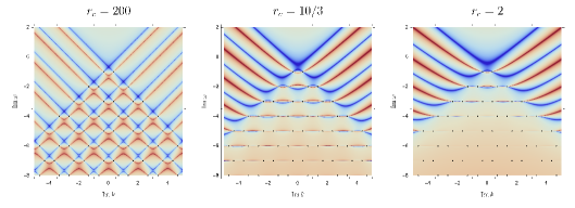
Figure 1: Heatmaps of the Green’s function in deformed CFTs dual to BTZ black holes with a finite radial cutoff. Red and blue lines denote the poles and zeros respectively, while black dots mark the pole-skipping points. From left to right, the location of the radial cutoff surface $r_{c}$ approaches the horizon, making higher-order poles and zeros increasingly difficult to distinguish.

Figure 2: The exterior of a black hole can be reconstructed from different subsets of boundary pole-skipping points (represented by black dots) by solving the linear system $\text{Det}(\vec{\mathcal{M}}^{(n)}(\textbf{g}))=0$. The green and red quadrilaterals enclose portions of two such subsets.

Moreover, our method reveals that the bulk metric is redundantly encoded in the boundary pole-skipping points, as illustrated schematically in Fig. 2. This redundancy arises from a set of $\mu$-polynomial constraints, such as $P_{n}(\mu)$ (18). Upon imposing these constraints, the remaining independent pole-skipping points precisely match the number of bulk degrees of freedom, namely $g_{vv_{n}}$ and $g_{vr_{n-1}}$. Importantly, these constraints are not exclusive to holographic theories; they can be derived under a general static, planar-symmetric black hole background, along with a class of master equation of the form $(\nabla^{2}+V(r))\Phi(r)=0$, whose pole-skipping structure aligns with the KG equation (2), without invoking holographic duality. Generalizing these constraints to spherical or hyperbolic black holes is straightforward. In the future, it would be intriguing to investigate the origin of these constraints from the field theory perspective in holographic setups and to explore their applicability to the energy density Green’s functions that exhibit chaotic pole-skipping points at the upper-half frequency plane.

Finally, owing to its analyticity and simplicity, our reconstruction method offers a compelling framework that could drive future experiments exploring the emergence of spacetime, e.g., the search for “spacetime-emergent materials” [67, 68]. However, directly locating the pole-skipping points experimentally may be challenging, as it is difficult to directly measure the retarded Green’s function with complex-valued frequency and momentum. Still, since real-frequency spectral functions can be reconstructed from imaginary-frequency Green’s functions via analytic continuation [69, 70], we expect that pole-skipping points can likewise be accessed from experimentally measurable Green’s functions with real frequency and momentum. Furthermore, we anticipate that pole-skipping data could eventually be extracted directly from quantum processor simulations of many-body systems .

Acknowledgments—We would like to thank Navid Abbasi, Xian-Hui Ge, Song He and Zhuo-Yu Xian for helpful discussions. A special thanks goes to Sašo Grozdanov and Mile Vrbica for their frequent and insightful discussions, as well as their valuable feedback on the draft of this Letter. SFW is supported by NSFC grants No.12275166 and No.12311540141.

References

- [1] E. Witten, Anti-de Sitter space and holography, Adv. Theor. Math. Phys. 2 (1998) 253–291 [arXiv:hep-th/9802150].
- [2] S. S. Gubser, I. R. Klebanov and A. M. Polyakov, Gauge theory correlators from noncritical string theory, Phys. Lett. B 428 (1998) 105–114 [arXiv:hep-th/9802109].
- [3] J. M. Maldacena, The Large N Limit of Superconformal Field Theories and Supergravity, International Journal of Theoretical Physics 38 (1999), no. 4 1113–1133 [arXiv:hep-th/9711200].
- [4] J. Casalderrey-Solana, H. Liu, D. Mateos, K. Rajagopal and U. Achim Wiedemann, Gauge/String Duality, Hot QCD and Heavy Ion Collisions. Cambridge University Press, 2014.
- [5] D. Harlow, Jerusalem Lectures on Black Holes and Quantum Information, Rev. Mod. Phys. 88 (2016) 015002 [arXiv:1409.1231].
- [6] M. Ammon and J. Erdmenger, Gauge/gravity duality: Foundations and applications. Cambridge University Press, Cambridge, 4, 2015.
- [7] J. Zaanen, Y.-W. Sun, Y. Liu and K. Schalm, Holographic Duality in Condensed Matter Physics. Cambridge Univ. Press, 2015.
- [8] S. A. Hartnoll, A. Lucas and S. Sachdev, Holographic quantum matter, arXiv:1612.07324.
- [9] S. de Haro, S. N. Solodukhin and K. Skenderis, Holographic reconstruction of space-time and renormalization in the AdS / CFT correspondence, Commun. Math. Phys. 217 (2001) 595–622 [arXiv:hep-th/0002230].
- [10] J. Hammersley, Extracting the bulk metric from boundary information in asymptotically AdS spacetimes, JHEP 12 (2006) 047 [arXiv:hep-th/0609202].
- [11] S. Bilson, Extracting spacetimes using the AdS/CFT conjecture, Journal of High Energy Physics 2008 (Aug., 2008) 073–073 [arXiv:0807.3695].
- [12] S. Bilson, Extracting Spacetimes using the AdS/CFT Conjecture: Part II, Journal of High Energy Physics 2011 (Feb., 2011) 50 [arXiv:1012.1812].
- [13] B. Czech, X. Dong and J. Sully, Holographic Reconstruction of General Bulk Surfaces, Journal of High Energy Physics 11 (2014) 015 [arXiv:1406.4889].
- [14] J. Hammersley, Extracting the bulk metric from boundary information in asymptotically AdS spacetimes, JHEP 12 (2006) 047 [arXiv:hep-th/0609202].
- [15] N. Engelhardt and G. T. Horowitz, Recovering the spacetime metric from a holographic dual, Adv. Theor. Math. Phys. 21 (2017) 1635–1653 [arXiv:1612.00391].
- [16] S. R. Roy and D. Sarkar, Bulk metric reconstruction from boundary entanglement, Physical Review D 98 (Sept., 2018) 066017 [arXiv:1801.07280].
- [17] K. Hashimoto, S. Sugishita, A. Tanaka and A. Tomiya, Deep learning and the AdS/CFT correspondence, Phys. Rev. D 98 (2018), no. 4 046019 [arXiv:1802.08313].
- [18] N. Bao, C. Cao, S. Fischetti and C. Keeler, Towards Bulk Metric Reconstruction from Extremal Area Variations, Class. Quant. Grav. 36 (2019), no. 18 185002 [arXiv:1904.04834].
- [19] Y.-K. Yan, S.-F. Wu, X.-H. Ge and Y. Tian, Deep learning black hole metrics from shear viscosity, Physical Review D 102 (Nov., 2020) 101902 [arXiv:2004.12112].
- [20] K. Hashimoto, Building bulk from Wilson loops, PTEP 2021 (2021), no. 2 023B04 [arXiv:2008.10883].
- [21] K. Hashimoto and R. Watanabe, Bulk reconstruction of metrics inside black holes by complexity, Journal of High Energy Physics 2021 (Sept., 2021) 165 [arXiv:2103.13186].
- [22] W.-B. Xu and S.-F. Wu, Reconstructing black hole exteriors and interiors using entanglement and complexity, Journal of High Energy Physics 2023 (July, 2023) 83 [arXiv:2305.01330].
- [23] B.-W. Fan and R.-Q. Yang, Inverse problem of correlation functions in holography, Journal of High Energy Physics 10 (2024) 228 [arXiv:2310.10419].
- [24] J. M. Maldacena, Eternal Black Holes in AdS, Journal of High Energy Physics 2003 (Apr., 2003) 021–021 [arXiv:hep-th/0106112].
- [25] S. Ryu and T. Takayanagi, Holographic Derivation of Entanglement Entropy from AdS/CFT, Physical Review Letters 96 (May, 2006) 181602 [arXiv:hep-th/0603001].
- [26] M. V. Raamsdonk, Building up spacetime with quantum entanglement, General Relativity and Gravitation 42 (Oct., 2010) 2323–2329 [arXiv:1005.3035].
- [27] B. Swingle, Entanglement Renormalization and Holography, Physical Review D 86 (Sept., 2012) [arXiv:0905.1317].
- [28] J. Maldacena and L. Susskind, Cool horizons for entangled black holes, Fortschritte der Physik 61 (Sept., 2013) 781–811 [arXiv:1306.0533].
- [29] S. Grozdanov, K. Schalm and V. Scopelliti, Black hole scrambling from hydrodynamics, Physical Review Letters 120 (June, 2018) 231601 [arXiv:1710.00921].
- [30] M. Blake, H. Lee and H. Liu, A quantum hydrodynamical description for scrambling and many-body chaos, Journal of High Energy Physics 2018 (Oct., 2018) 127 [arXiv:1801.00010].
- [31] M. Blake, R. A. Davison, S. Grozdanov and H. Liu, Many-body chaos and energy dynamics in holography, Journal of High Energy Physics 2018 (Oct., 2018) 35 [arXiv:1809.01169].
- [32] M. Knysh, H. Liu and N. Pinzani-Fokeeva, New horizon symmetries, hydrodynamics, and quantum chaos, Journal of High Energy Physics 09 (2024) 162 [arXiv:2405.17559].
- [33] W. Z. Chua, T. Hartman and W. W. Weng, Replica manifolds, pole skipping, and the butterfly effect, arXiv:2504.08139.
- [34] M. Blake, R. A. Davison and D. Vegh, Horizon constraints on holographic Green’s functions, Journal of High Energy Physics 2020 (Jan., 2020) 77 [arXiv:1904.12883].
- [35] D. Wang and Z.-Y. Wang, Pole skipping in holographic theories with bosonic fields, Physical Review Letters 129 (Nov., 2022) 231603 [arXiv:2208.01047].
- [36] S. Ning, D. Wang and Z.-Y. Wang, Pole skipping in holographic theories with gauge and fermionic fields, Journal of High Energy Physics 2023 (Dec., 2023) 84 [arXiv:2308.08191].
- [37] F. M. Haehl and M. Rozali, Effective Field Theory for Chaotic CFTs, Journal of High Energy Physics 10 (2018) 118 [arXiv:1808.02898].
- [38] S. Grozdanov, On the connection between hydrodynamics and quantum chaos in holographic theories with stringy corrections, Journal of High Energy Physics 01 (2019) 048 [arXiv:1811.09641].
- [39] S. Grozdanov, P. K. Kovtun, A. O. Starinets and P. Tadić, The complex life of hydrodynamic modes, Journal of High Energy Physics 2019 (Nov., 2019) 97 [arXiv:1904.12862].
- [40] M. Natsuume and T. Okamura, Pole-skipping with finite-coupling corrections, Physical Review D 100 (Dec., 2019) 126012 [arXiv:1909.09168].
- [41] X. Wu, Higher curvature corrections to pole-skipping, Journal of High Energy Physics 2019 (Dec., 2019) 140 [arXiv:1909.10223].
- [42] N. Ceplak, K. Ramdial and D. Vegh, Fermionic pole-skipping in holography, Journal of High Energy Physics 2020 (July, 2020) 203 [arXiv:1910.02975].
- [43] S. Grozdanov, Bounds on transport from univalence and pole-skipping, Physical Review Letters 126 (Feb., 2021) 051601 [arXiv:2008.00888].
- [44] D. M. Ramirez, Chaos and pole skipping in CFT2, Journal of High Energy Physics 12 (2021) 006 [arXiv:2009.00500].
- [45] C. Choi, M. Mezei and G. Sárosi, Pole skipping away from maximal chaos, Journal of High Energy Physics 2021 (Feb., 2021) 207 [arXiv:2010.08558].
- [46] Y. Ahn, V. Jahnke, H.-S. Jeong, K.-Y. Kim, K.-S. Lee and M. Nishida, Classifying pole-skipping points, Journal of High Energy Physics 2021 (Mar., 2021) 175 [arXiv:2010.16166].
- [47] M. Natsuume and T. Okamura, Pole-skipping and zero temperature, Phys. Rev. D 103 (2021), no. 6 066017 [arXiv:2011.10093].
- [48] H. Yuan and X.-H. Ge, Pole-Skipping and Hydrodynamic Analysis in Lifshitz, and Rindler Geometries, Journal of High Energy Physics 2021 (June, 2021) 165 [arXiv:2012.15396].
- [49] N. Abbasi and M. Kaminski, Constraints on quasinormal modes and bounds for critical points from pole-skipping, Journal of High Energy Physics 03 (2021) 265 [arXiv:2012.15820].
- [50] M. Blake and R. A. Davison, Chaos and pole-skipping in rotating black holes, Journal of High Energy Physics 01 (2022) 013 [arXiv:2111.11093].
- [51] M. Baggioli, S. Grieninger, S. Grozdanov and Z. Lu, Aspects of univalence in holographic axion models, Journal of High Energy Physics 2022 (Nov., 2022) 32 [arXiv:2205.06076].
- [52] S. Grozdanov and M. Vrbica, Pole-skipping of gravitational waves in the backgrounds of four-dimensional massive black holes, Eur. Phys. J. C 83 (2023), no. 12 1103 [arXiv:2303.15921].
- [53] M. Natsuume and T. Okamura, Pole skipping in a non-black-hole geometry, Phys. Rev. D 108 (2023), no. 4 046012 [arXiv:2306.03930].
- [54] S. Grozdanov, T. Lemut and J. F. Pedraza, Reconstruction of the quasinormal spectrum from pole-skipping, Physical Review D 108 (Nov., 2023) L101901 [arXiv:2308.01371].
- [55] A. Almheiri, X. Dong and D. Harlow, Bulk Locality and Quantum Error Correction in AdS/CFT, Journal of High Energy Physics 04 (2015) 163 [arXiv:1411.7041].
- [56] Z. Lu, C. Ran and S.-F. Wu, The algebraic structure underlying pole-skipping points (coming soon), .
- [57] I. G. Macdonald, Symmetric Functions and Hall Polynomials. Oxford Mathematical Monographs. Oxford University Press, second edition, second edition ed.
- [58] X. Dong, S. Harrison, S. Kachru, G. Torroba and H. Wang, Aspects of holography for theories with hyperscaling violation, Journal of High Energy Physics 2012 (June, 2012) 41 [arXiv:1201.1905].
- [59] W. Chemissany and I. Papadimitriou, Generalized dilatation operator method for non-relativistic holography, Phys. Lett. B 737 (2014) 272–276 [arXiv:1405.3965].
- [60] H. Kodama and A. Ishibashi, A master equation for gravitational perturbations of maximally symmetric black holes in higher dimensions, Progress of Theoretical Physics 110 (Oct., 2003) 701–722 [arXiv:hep-th/0305147].
- [61] H. Kodama and A. Ishibashi, Master equations for perturbations of generalised static black holes with charge in higher dimensions, Progress of Theoretical Physics 111 (Jan., 2004) 29–73 [arXiv:hep-th/0308128].
- [62] A. Jansen, A. Rostworowski and M. Rutkowski, Master equations and stability of Einstein-Maxwell-scalar black holes, Journal of High Energy Physics 2019 (Dec., 2019) 36 [arXiv:1909.04049].
- [63] Factorial expressions should be simplified before substituting specific values of .
- [64] A. Cavaglià, S. Negro, I. M. Szécsényi and R. Tateo, -deformed 2D Quantum Field Theories, Journal of High Energy Physics 10 (2016) 112 [arXiv:1608.05534].
- [65] F. A. Smirnov and A. B. Zamolodchikov, On space of integrable quantum field theories, Nuclear Physics B 915 (Feb., 2017) 363–383 [arXiv:1608.05499].
- [66] L. McGough, M. Mezei and H. Verlinde, Moving the CFT into the bulk with , Journal of High Energy Physics 04 (2018) 010 [arXiv:1611.03470].
- [67] K. Hashimoto, D. Takeda, K. Tanaka and S. Yonezawa, Spacetime-emergent ring toward tabletop quantum gravity experiments, Phys. Rev. Res. 5 (Jun, 2023) 023168 [arXiv:2211.13863].
- [68] K. Hashimoto, K. Matsuo, M. Murata, G. Ogiwara and D. Takeda, Machine-learning emergent spacetime from linear response in future tabletop quantum gravity experiments, Mach. Learn. Sci. Tech. 6 (2025), no. 1 015030 [arXiv:2411.16052].
- [69] M. Jarrell and J. E. Gubernatis, Bayesian inference and the analytic continuation of imaginary-time quantum Monte Carlo data, Phys. Rept. 269 (1996) 133–195.
- [70] H. Shao and A. W. Sandvik, Progress on stochastic analytic continuation of quantum Monte Carlo data, Phys. Rept. 1003 (2023) 1–88 [arXiv:2202.09870].
- [71] See a recent simulation framework based on linear response theory [72].
- [72] E. Kökcü, H. A. Labib, J. K. Freericks and A. F. Kemper, A linear response framework for quantum simulation of bosonic and fermionic correlation functions, Nature Commun. 15 (2024), no. 1 3881 [arXiv:2302.10219].