Studying Maximal Entanglement and Bell Nonlocality at an Electron-Ion Collider

Abstract

In this paper, we propose to test quantum entanglement and Bell nonlocality at an Electron-Ion Collider (EIC). By computing the spin correlations in quark-antiquark pairs produced via photon-gluon fusion, we find that longitudinally polarized photons produce maximal entanglement at leading order, while transversely polarized photons generate significant entanglement near the threshold and in the ultra-relativistic regime. Compared to hadron colliders, the EIC provides a cleaner experimental environment for measuring entanglement through the $\gamma^{\ast}g\to q\bar{q}$ channel, offering a strong signal and a promising avenue to verify Bell nonlocality. This study extends entanglement measurements to the EIC, presenting new opportunities to explore the interplay of quantum information phenomena and hadronic physics in the EIC era.

Introduction.— As the quintessential phenomenon of quantum mechanics, quantum entanglement has historically been pivotal in establishing the probabilistic interpretation of quantum theory and revealing the genuinely non-local nature of quantum mechanics.

In 1935, the famous Einstein-Podolsky-Rosen (EPR) paradox Einstein et al. (1935) was proposed as a challenge to the concept of entanglement and, more broadly, the orthodox Copenhagen interpretation of quantum mechanics. The EPR paradox suggested that quantum mechanics might be incomplete and raised the possibility of alternative interpretations based on hidden variables. Hidden variable theories aim to provide additional information, offering a complete, deterministic description of physical systems without relying on probabilistic concepts. For many years, it was believed that hidden variable theories and quantum mechanics would yield identical physical predictions, making it impossible to experimentally distinguish between them. In 1964, Bell ingeniously demonstrated that any local hidden variable theory is fundamentally incompatible with quantum mechanics through what is now known as the Bell inequality Bell (1964). A few years later, Clauser, Horne, Shimony, and Holt Clauser et al. (1969); Clauser and Horne (1974) proposed the Clauser-Horne-Shimony-Holt (CHSH) inequality, which generalized the Bell inequality and laid the foundation for a practical framework for experimental tests at the atomic level. Their work not only provided decisive evidence supporting quantum mechanics and rejecting local hidden variable theories but also paved the way for the development of the field of quantum information theory (see Plenio and Virmani (2007); Wootters (1998); Cerf and Adami (1998); Acin et al. (2002); Cirelson (1980); Horodecki et al. (1995), among many other references).

Recently, the study of quantum entanglement in high-energy collisions Tu et al. (2020); Datta et al. (2025); Hentschinski et al. (2023); Florio et al. (2023); Uwer (2005); Afik and de Nova (2023, 2022, 2021); Hayrapetyan et al. (2023); Cheng et al. (2024); Aguilar-Saavedra (2024a); Chen et al. (2013); Wu et al. (2024a); Ashby-Pickering et al. (2023); Barr et al. (2024); Ehatäht et al. (2024); Guo et al. (2025); Morales (2023); Parke and Shadmi (1996); Ruzi et al. (2024); Aguilar-Saavedra (2023a); Altakach et al. (2023); Aoude et al. (2024); Bernal (2024); Brandenburg et al. (2002); Heinrich et al. (2022); Hentschinski et al. (2024); James et al. (2001); Kowalska and Sessolo (2024); Li et al. (2023); Ma and Li (2024); Maltoni et al. (2024); Sakurai and Spannowsky (2024); Severi and Vryonidou (2023); Subba and Rahaman (2024); Severi et al. (2022); Wu et al. (2024b); Kharzeev and Levin (2017); Aguilar-Saavedra and Casas (2024); Grabarczyk (2024); Fabbrichesi et al. (2024a, b); Li et al. (2024); Shi (2004); Fabbri et al. (2024); Bramon and Garbarino (2002); Wu et al. (2024c); Mahlon and Parke (1996); Dong et al. (2024); Aguilar-Saavedra et al. (2023); Aguilar-Saavedra and Casas (2022); Bernal et al. (2023, 2024); Bi et al. (2024); Fabbrichesi and Marzola (2024); Fabbrichesi et al. (2023); Ghosh and Sharma (2023); Grabarczyk (2024); White and White (2024); Han et al. (2024); Du et al. (2024); Cheng and Yan (2025); Morales (2024) has attracted significant attention, and new opportunities to explore this fascinating phenomenon beyond the atomic scale have emerged. Both experimentalists and theorists have been exploring the production of top-antitop quark pair at the Large Hadron Collider (LHC), carrying out a meticulous experimental measurement Sirunyan et al. (2019); Aaboud et al. (2020); Aad et al. (2024); Hayrapetyan et al. (2024) of entanglement by studying the correlation between their weak decay productsAguilar-Saavedra (2023b, 2024b). In particular, the ATLAS and CMS Collaborations Aad et al. (2024); Hayrapetyan et al. (2024) at the LHC have observed quantum entanglement between top quark pairs in proton-proton collisions at $\sqrt{s}=13$ TeV. Typically, top quark pairs are produced via quark annihilation or gluon-gluon fusion channels. By measuring the angular correlations of the lepton pairs in top’s weak decay products, one can access the transferred spin information. However, due to the contribution from the quark annihilation channelSeveri et al. (2022); Fabbrichesi et al. (2025), it remains challenging to observe violations of Bell inequality or Bell nonlocality at the LHC.

As summarized in a recent article Afik et al. (2025), there have been many studies positioned at the interplay between quantum information theory and high-energy physics, examining various channels in electron-positron annihilation processes at dedicated colliders and in proton-proton collisions at the LHC. However, theoretical studies of electron-proton collisions are still lacking, and complementary measurements at the upcoming Electron-Ion Collider (EIC) Accardi et al. (2016); Abdul Khalek et al. (2022); Anderle et al. (2021) could potentially become significant. We find that the quark pair produced by a longitudinal virtual photon is always maximally entangled at leading order (LO), and the pair produced by a transverse photon is in a maximally entangled spin-singlet state near the threshold. This makes EICs ideal machines for measuring entanglement and Bell nonlocality.

This paper is structured as follows: we first introduce the general formalism for the density matrix of a two-qubit system and the criteria for quantum entanglement, then compute the spin density matrix for the quark-antiquark pair in the photon-gluon fusion process. Additionally, we present results for both longitudinal and transverse incident photons separately and demonstrate that entanglement and Bell nonlocality can be measured at the EIC. Finally, we comment on the experimental implications and possible future extensions of this work.

General formalism.— Without loss of generality, any 2-qubit system (such as a quark-antiquark pair) can be represented by a $4\times 4$ spin density matrix as follows

$$\rho=\frac{1}{4}(\mathds{1}_{4}+B^{+}_{i}\sigma^{i}\otimes\mathds{1}_{2}+B^{-}_{j}\mathds{1}_{2}\otimes\sigma^{j}+C_{ij}\sigma^{i}\otimes\sigma^{j}),$$ (1)

where $B^{+}_{i}=\tr[\rho(\sigma^{i}\otimes\mathds{1}_{2})]$ and $B^{-}_{j}=\tr[\rho(\mathds{1}_{2}\otimes\sigma^{j})]$ are the spin polarizations of each qubit, and $C_{ij}=\tr[\rho(\sigma^{i}\otimes\sigma^{j})]$ is a measure of the spin correlation between qubits. For example, $C_{ij}=-\delta_{ij}$ indicates that the two spins are always anti-parallel and therefore form a spin singlet configuration $\ket{\Psi^{-}}=\frac{1}{\sqrt{2}}(\ket{\uparrow\downarrow}-\ket{\downarrow\uparrow})$. Similarly, correlation matrices with $C=\text{diag}(1,1,-1),\text{diag}(1,-1,1),\text{diag}(-1,1,1)$ correspond to the spin triplet states and the other three Bell states, i.e., $\ket{\Psi^{+}}=\frac{1}{\sqrt{2}}(\ket{\uparrow\downarrow}+\ket{\downarrow\uparrow})$ and $\ket{\Phi^{\pm}}=\frac{1}{\sqrt{2}}(\ket{\uparrow\uparrow}\pm\ket{\downarrow\downarrow})$.

To quantify the entanglement, one can define the following entanglement signatures for 2-qubit systems. A state is separable iff there exists $p_{k}\geq 0$ for which

$$\rho=\sum_{k}p_{k}\rho^{a}_{k}\otimes\rho^{b}_{k}\quad\text{with}\quad\sum_{k}p_{k}=1,$$ (2)

and an entangled state is defined as a non-separable state. To determine if a mixed state is entangled, one can employ the Peres-Horodecki criterion Peres (1996); Horodecki (1997). It states that if a mixed state $\rho$ is separable, its partial transpose

$$\rho^{T_{2}}=\sum_{k}p_{k}\rho^{a}_{k}\otimes\left(\rho^{b}_{k}\right)^{T}$$ (3)

is non-negative. Thus, if one of the eigenvalues of $\rho^{T_{2}}$ is negative, the state $\rho$ is entangled. Moreover, for a 2-qubit system, this is a sufficient and necessary condition for entanglement.

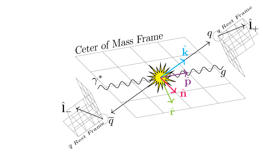
Figure 1: Illustration of the helicity basis vectors ${\hat{\mathbf{n}},\hat{\mathbf{r}},\hat{\mathbf{k}}}$ and the unit vector $\hat{\mathbf{p}}$ of the photon momentum, defined in the center-of-mass frame, alongside the unit vectors ${\hat{\mathbf{l}}+,\hat{\mathbf{l}}-}$ of the fermionic decay products (indicating momentum directions), shown in their respective parent particle rest frames, where the spin of each particle and the decay spin density matrices are also conventionally defined.

As we will show in later calculations, it is convenient to choose the Cartesian coordinates in the center-of-mass frame as shown in Fig. 1, and express the quark pair production results in the helicity basis $\{\hat{\mathbf{n}},\hat{\mathbf{r}},\hat{\mathbf{k}}\}$. In this coordinate system, the coefficients $C_{nr},C_{rn},C_{nk},C_{kn}$, $B^{\pm}_{i}$ vanish. Therefore, in this coordinate system, according to the Peres-Horodecki criterion, at least one of the following must be positive for the state to be entangled:

$$\Delta_{1}=-1+C_{nn}+\sqrt{(C_{rr}-C_{kk})^{2}+(C_{rk}+C_{kr})^{2}},\quad$$ (4)

$$\Delta_{2}=-1-C_{nn}+\sqrt{(C_{rr}+C_{kk})^{2}+(C_{rk}-C_{kr})^{2}}.\quad$$ (5)

The corresponding concurrence is then given by:

$$\mathcal{C}[\rho]=\max\left\{\Delta_{1}/2,\Delta_{2}/2,0\right\}.$$ (6)

The concurrence, $\mathcal{C}[\rho]$, is a key quantity for characterizing entanglement, with values ranging between $0$ and $1$. A value of $\mathcal{C}[\rho]=0$ corresponds to a separable state, while $\mathcal{C}[\rho]=1$ indicates a maximally entangled state. It is formally defined as Wootters (1998): $\mathcal{C}[\rho]=\max\{0,\lambda_{1}-\lambda_{2}-\lambda_{3}-\lambda_{4}\}$, where $\lambda_{i}$ are the eigenvalues of the Hermitian matrix $\mathcal{R}=\sqrt{\sqrt{\rho}\tilde{\rho}\sqrt{\rho}}$ in decreasing order, and the spin-flipped density matrix is $\tilde{\rho}=(\sigma^{y}\otimes\sigma^{y})\rho^{*}(\sigma^{y}\otimes\sigma^{y})$. In the case considered in this work, the expression given in Eq. (6) coincides with the formal definition above.

Furthermore, if the matrix $C_{ij}$ is symmetric ($C_{rk}=C_{kr}$) with $C_{nn}<0$, the sufficient condition for entanglement is $\Delta_{2}>0$ Afik and de Nova (2021, 2022); Aad et al. (2024); Hayrapetyan et al. (2024) where

$$\Delta=-1-C_{nn}+|C_{rr}+C_{kk}|.$$ (7)

Furthermore, if $C_{rr}$ and $C_{kk}$ are also nonpositive (e.g., $C=\text{diag}(-1,-1,-1)$ for the spin singlet state), one finds $\Delta=-\tr C-1$. Thus, we obtain another sufficient condition for entanglement: $D<-1/3$, where $D=\tr C/3$. This quantity can be measured directly in experiments, as $D=-3\langle\cos\varphi\rangle$, with $\cos\varphi\equiv\hat{\mathbf{l}}_{+}\cdot\hat{\mathbf{l}}_{-}$Aad et al. (2024); Hayrapetyan et al. (2024), by measuring the decayed leptons from the entangled top quark pairs near the threshold.

In classical local hidden variable theories, one form of Bell inequalityBell (1964) is given by

$$\mathcal{B}=|\langle a_{1}b_{1}\rangle+\langle a_{2}b_{1}\rangle+\langle a_{1}b_{2}\rangle-\langle a_{2}b_{2}\rangle|\leq 2,$$ (8)

where the values of $a_{1},a_{2},b_{1},b_{2}$ can either be $1$ or $-1$. This inequality can be demonstrated by considering all possible cases. Given the density matrix correlation coefficients $C_{ij}$, one can rewrite the expectation value $\langle a_{1}b_{1}\rangle$ as $\text{tr}[\rho\hat{a}_{1}\cdot\vec{\sigma}\otimes\hat{b}_{1}\cdot\vec{\sigma}]=\hat{a}_{1}\cdot C\cdot\hat{b}_{1}$ and then express the generalized Bell inequality (CHSH inequality)Clauser et al. (1969); Clauser and Horne (1974) as Fabbrichesi et al. (2021)

$$\mathcal{B}=|\hat{a}_{1}\cdot C\cdot(\hat{b}_{1}+\hat{b}_{2})+\hat{a}_{2}\cdot C\cdot(\hat{b}_{1}-\hat{b}_{2})|\leq 2,$$ (9)

where $\hat{a}_{1,2}$ and $\hat{b}_{1,2}$ are the unit vectors along which the quark and antiquark spins can be measured, respectively. Remarkably, it can be shown through algebraic derivation that $\mathcal{B}\leq 2\sqrt{2}$ for a quantum system, and the maximally entangled state can achieve the maximum value of $2\sqrt{2}$. Therefore there exists a range $2<\mathcal{B}\leq 2\sqrt{2}$ which violates the Bell inequality. The violation of the Bell inequality indicates the presence of Bell nonlocality in quantum mechanics, and it is equivalent toCirelson (1980); Horodecki et al. (1995)

$$\mathcal{N}[\rho]\equiv\mu_{1}+\mu_{2}-1>0,$$ (10)

where $\mu_{1}\geq\mu_{2}\geq\mu_{3}$ are the eigenvalues of the matrix $C^{T}C$ in descending order. In principle, since all elements of the correlation matrix $C$ can be measured, one can test the Bell nonlocality experimentally through Eq. (10). For Bell states, which maximally violate the Bell inequality, it gives the nonlocality measure $\mathcal{N}=1$.

Quark Pair Productions in photon-gluon fusions.— Following the convention used in Refs. Uwer (2005); Afik and de Nova (2023); Bernreuther and Brandenburg (1994); Bernreuther et al. (1998); Brandenburg et al. (1999); Baumgart and Tweedie (2013); Bernreuther et al. (2015); Afik and de Nova (2022, 2021); Aoude et al. (2022), we define the unnormalized spin density matrix for the process $\gamma^{*}g\to q\overline{q}$ as

$$R_{\alpha\alpha^{\prime},\beta\beta^{\prime}}=\frac{1}{N}\sum_{\text{color, spin}}\mathcal{M}^{\ast}_{\gamma^{*}g\to q^{\alpha}\overline{q}^{\alpha^{\prime}}}\mathcal{M}_{\gamma^{*}g\to q^{\beta}\overline{q}^{\beta^{\prime}}},$$ (11)

where $1/N$ represents the average over the intial state color and spin, and $\alpha,\beta,\alpha^{\prime},\beta^{\prime}$ are open spinor indices of quarks and antiquarks produced in the final state. Using the LO scattering amplitude $\mathcal{M}_{\gamma^{*}g\to q^{\alpha}\overline{q}^{\alpha^{\prime}}}$, it is straightforward to obtain the spin density matrix in an analytical form. Similar to Eq. (1), since $R$ is a $4\times 4$ Hermitian matrix, it takes the form

$$R=\tilde{A}\mathds{1}_{4}+\tilde{B}^{+}_{i}\sigma^{i}\otimes\mathds{1}_{2}+\tilde{B}^{-}_{j}\mathds{1}_{2}\otimes\sigma^{j}+\tilde{C}_{ij}\sigma^{i}\otimes\sigma^{j},$$ (12)

where the overall normalization $\tilde{A}=\tr R/4$ is proportional to the differential cross-section, and the rest of $R$ is related to $\rho$ as follows: $\rho=R/\tr R=R/(4\tilde{A})$, thus $B^{\pm}_{i}=\tilde{B}^{\pm}_{i}/\tilde{A}$ and $C_{ij}=\tilde{C}_{ij}/\tilde{A}$. In the above expression for $R$, we have suppressed the spinor indices, which can be recovered as, for example, for the last term as $\tilde{C}_{ij}\sigma^{i}_{\alpha\beta}\otimes\sigma^{j}_{\alpha^{\prime}\beta^{\prime}}$ with the first Pauli matrix carrying the quark spinor indices and the second carrying the antiquark spinor indices.

The $R$-matrix and these coefficients can be calculated explicitly in the center-of-mass frame of the quark pair with the helicity basis $\{\hat{\mathbf{n}},\hat{\mathbf{r}},\hat{\mathbf{k}}\}$ where $\hat{\mathbf{k}}$ is the direction of the outgoing quark, $\hat{\mathbf{n}}$ is orthogonal to the production plane, and $\hat{\mathbf{r}}$ is orthogonal to the $\{\hat{\mathbf{n}},\hat{\mathbf{k}}\}$ plane as shown in Fig. 1. The indicies $i$ and $j$ of Pauli matrices, which run from $1$ to $3$, are then mapped to the $\{\hat{\mathbf{n}},\hat{\mathbf{r}},\hat{\mathbf{k}}\}$ coordinates as well. In the center-of-mass frame, let $p,p^{\prime},k,k^{\prime}$ be the 4-momenta of the photon, the gluon, the quark, and the antiquark, respectively. The incoming photons are mostly off-shell, thus we write $p^{2}=-Q^{2}<0$. The invariant mass $\sqrt{\hat{s}}$ is defined from the Mandelstam variable $\hat{s}=(p+p^{\prime})^{2}=(k+k^{\prime})^{2}$, which is the partonic center-of-mass energy. To make the final expression more compact, we define three more dimensionless variables: $\alpha=Q^{2}/\hat{s}$, $\beta=\sqrt{1-4m^{2}/\hat{s}}$, and $z=\hat{\mathbf{p}}\cdot\hat{\mathbf{k}}$, where $\alpha$ is related to virtuality, $\beta$ is the speed of the produced quark, and $z=\cos\theta$ with $\theta$ being the angle between $\hat{\mathbf{p}}$ and $\hat{\mathbf{k}}$.

In deep inelastic scattering at EICs, the incoming photons are spacelike virtual photons, which can be either longitudinal or transverse. Typically, the measured unpolarized cross-sections are a linear combination of these two contributions. In EIC experiments, it is potentially possible to separate these two contributions, despite the associated challenges. Below, we present the cases of longitudinal and transverse photons separately, highlighting their interestingly distinct features. Again, we choose to work in the $\{\hat{\mathbf{n}},\hat{\mathbf{r}},\hat{\mathbf{k}}\}$ coordinate system, using the physical longitudinal and transverse polarization vectors, $\epsilon_{L}$ and $\epsilon_{T}$, respectively, such that $\epsilon\cdot p=0$.

Figure 2: Examples of spin configurations of the longitudinal and transverse photon channels at $\theta=\frac{\pi}{2}$ ($z=0$) and the production threshold $\beta=0$.

For the longitudinal polarization contribution, we find that the coefficient matrix $C$ is given by

$$C=\begin{pmatrix}1&0&0\\ 0&-\chi_{1}&-\chi_{2}\\ 0&-\chi_{2}&\chi_{1}\end{pmatrix}$$ (13)

with $$\chi_{1}=\frac{1-2z^{2}+z^{2}\beta^{2}}{1-z^{2}\beta^{2}},$$ (15)

$$\chi_{2}=\frac{2z\sqrt{(1-z^{2})(1-\beta^{2})}}{1-z^{2}\beta^{2}}.$$

Note that $\chi_{1}^{2}+\chi_{2}^{2}=1$. In this case, the concurrence $\mathcal{C}[\rho_{L}]\equiv 1$ and the nonlocality measure $\mathcal{N}[\rho_{L}]=1$, indicating maximal entanglement and maximal violation of Bell inequality. We find that the quark pair in a maximally entangled spin triplet state and the corresponding density matrix is always in the form of a pure state $\rho_{L}=\ket{\Psi}\bra{\Psi}$, where

$$\ket{\Psi}=\frac{1}{2}(\sqrt{1+\chi_{1}},\mathrm{i}\sqrt{1-\chi_{1}},\mathrm{i}\sqrt{1-\chi_{1}},\sqrt{1+\chi_{1}}).$$ (16)

For example as illustrated in Fig. 2, when $z=0$ ($\theta=\pi/2$), one finds $C=\mathrm{diag}(1,-1,1)$, which indicates $\ket{\Psi}=\ket{\Phi^{+}}$ and $\rho_{L}=\ket{\Phi^{+}}\bra{\Phi^{+}}$ where $\ket{\Phi^{+}}=(\ket{\uparrow\uparrow}+\ket{\downarrow\downarrow})/\sqrt{2}$. Interestingly, we also find the same $\rho$ for $\beta=1$ as in the relativistic limit.

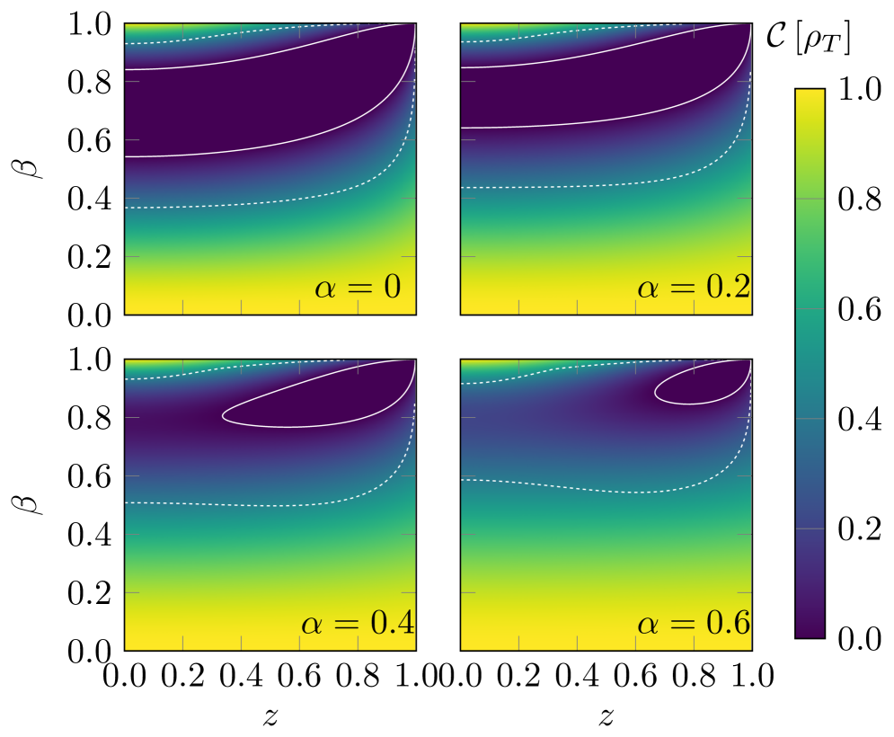
Figure 3: Density plots of the concurrence for the transverse polarized photon contribution at EIC as functions of quark velocity $\beta$ and the scalar projection $z$ at given values of the virtuality parameter $\alpha$, where solid lines and dashed lines indicate the boundaries for entanglement ($\mathcal{C}[\rho_{T}]=0$) and Bell nonlocality ($\mathcal{N}[\rho_{T}]=0$), respectively.

As to the transverse photon contribution, we find the density matrix is generally in a complicated mixed state. Due to its complexity, the full expression for the transverse contribution, which is presented in the appendix, is used to plot the concurrence $\mathcal{C}[\rho_{T}]$ in Fig. 3 as functions of $\beta$ and $z$ for given values of $\alpha$. It indicates that there is also a wide range of kinematics for observing entanglement and nonlocality.

Regarding the analytic results for the transverse contribution, if the photon is set to be on-shell ($\alpha=0$), then the non-vanishing coefficients of $R$ are:

$$\tilde{A} = F\left[1+2\beta^{2}(1-z^{2})-\beta^{4}(2-2z^{2}+z^{4})\right],$$ (17)

$$\tilde{C}_{nn} = -F\left[1-2\beta^{2}+\beta^{4}(2-2z^{2}+z^{4})\right],$$ (18)

$$\tilde{C}_{rr} = -F\left[1-\beta^{2}(2-\beta^{2})(2-2z^{2}+z^{4})\right],$$ (19)

$$\tilde{C}_{kk} = -F\left[1-2\beta^{2}z^{2}(1-z^{2})-\beta^{4}(2-2z^{2}+z^{4})\right],\quad$$ (20)

$$\tilde{C}_{kr} = \tilde{C}_{rk}=2F\beta^{2}\sqrt{1-\beta^{2}}z(1-z^{2})^{3/2},$$ (22)

$$\text{with}\quad F=\frac{e^{2}_{Q}g^{2}_{s}}{(1-\beta^{2}z^{2})^{2}}.$$

These coefficients are very similar to the ones of the process $gg\to q\overline{q}$Afik and de Nova (2022, 2021, 2023); Baumgart and Tweedie (2013); Bernreuther et al. (2015); Aoude et al. (2022), while only the factor $F$ is different. Notably, the matrix $\tilde{C}$ is not symmetric in the case of virtual photons ($\alpha>0$).

Let us comment on the two asymptotic limits for the transverse contribution to illustrate the relevant physics. At the production threshold, which is equivalent to the nonrelativistic limit by setting $\beta=0$, the spin correlation is then found to be $C_{ij}=-\delta_{ij}$ which gives $\rho_{T}=\ket{\Psi^{-}}\bra{\Psi^{-}},$ where $\ket{\Psi^{-}}$ is the spin singlet state. To understand this result, we note that the amplitude indicates that the transverse photon and gluon form a spin singlet state. In addition, the produced quarks are emitted without angular dependence in an s-wave with zero orbital angular momentum. In this case, conservation of angular momentum requires that the spin of the final state $q\bar{q}$ pair be zero. Meanwhile, in the high energy limit and near $z=0$ region, it is found that $q\bar{q}$ is in the spin triplet $\ket{\Phi^{-}}$ state due to the orbital angular momentum contribution. As expected, this result is in agreement with that in the $gg\to q\bar{q}$ channelAfik and de Nova (2021, 2022).

At the end, to measure the spin configuration of the quark pair, one can utilize the self-analyzing property of weak decays, as the momentum distributions of the decay products are correlated with the spins of the parent particles. Let ${\hat{\mathbf{l}}+,\hat{\mathbf{l}}-}$ represent the direction vectors of fermions produced in weak decays, measured in the rest frames of their respective parent particles, as illustrated in Fig. 1. The cross-section for producing the lepton pair can be expressed as

$$\frac{\differential\sigma}{\differential\Omega_{+}\differential\Omega_{-}}\propto\tr\left[(\Gamma_{+}\otimes\Gamma_{-})R\right],$$ (23)

where $\Gamma_{\pm}$ represents the decay density matrices for $q\bar{q}\to l^{+}+l^{-}+X$ in the rest frames of the parent particles, defined as followsBaumgart and Tweedie (2013):

$$\Gamma_{\pm}=\frac{\mathds{1}_{2}+\kappa_{\pm}(\hat{\mathbf{l}}_{\pm}\cdot\bm{\sigma})}{2},$$ (24)

where $\kappa_{+}$ and $\kappa_{-}$ are the spin-analyzing powers. Since $\Gamma_{\pm}$ depends on the dot product between the Pauli matrices $\sigma^{i}$ and the lepton’s direction, and given that $\tr[\sigma^{i}]=0$ and $\tr[\sigma^{i}\sigma^{j}]=2\delta^{ij}$, we can see that the spin information is transferred to the lepton’s motion by taking the trace of $(\Gamma_{+}\otimes\Gamma_{-})R$. Consequently, as the produced $q\bar{q}$ pair is unpolarized with $B^{\pm}=0$, we can obtain the normalized cross-section

$$\frac{1}{\sigma}\frac{\differential\sigma}{\differential\Omega_{+}\differential\Omega_{-}}=\frac{1+\kappa_{+}\kappa_{-}\hat{\mathbf{l}}_{+}\cdot C\cdot\hat{\mathbf{l}}_{-}}{(4\pi)^{2}}.$$ (25)

The correlation coefficients of the matrix $C$ can be determined by measuring the weighted angle averagesBernreuther et al. (2015); Fabbrichesi et al. (2021)

$$C_{ab}=\frac{9}{\kappa_{+}\kappa_{-}}\;\frac{1}{\sigma}\int_{-1}^{1}\differential\xi_{ab}\frac{\differential\sigma}{\differential\xi_{ab}}\xi_{ab}=\frac{9}{\kappa_{+}\kappa_{-}}\langle\xi_{ab}\rangle,$$ (26)

with the variable $\xi_{ab}=(\hat{\mathbf{l}}_{+}\cdot\hat{\mathbf{a}})(\hat{\mathbf{l}}_{-}\cdot\hat{\mathbf{b}})$, where the vectors $\hat{\mathbf{a}},\hat{\mathbf{b}}$ can be chosen to align with the helicity basis $\{\hat{\mathbf{n}},\hat{\mathbf{r}},\hat{\mathbf{k}}\}$. As a special example, the averaged trace $D=\text{tr}C/3$ can be obtained throughAad et al. (2024); Hayrapetyan et al. (2024)

$$D = \frac{3}{\kappa_{+}\kappa_{-}}\;\frac{1}{\sigma}\int_{-1}^{1}\differential\cos\varphi\frac{\differential\sigma}{\differential\cos\varphi}\cos\varphi$$ (27)

$$= \frac{3}{\kappa_{+}\kappa_{-}}\langle\cos\varphi\rangle.$$

where $\varphi$ is the relative angle between $\hat{\mathbf{l}}_{+}$ and $\hat{\mathbf{l}}_{-}$ that $\cos\varphi=\hat{\mathbf{l}}_{+}\cdot\hat{\mathbf{l}}_{-}$. Possible measurements of $C_{ij}$ can be cast into two categories as follows:

• Heavy quark pair channels such as $b\overline{b}$ or $c\overline{c}\rightarrow(l^{+}\nu q)(l^{-}\bar{\nu}\bar{q})$: By measuring the lepton pair in the decay product, one can extract the transferred spin correlation information from the heavy quark pair, thereby studying the entanglement and Bell nonlocality at an EIC. (For similar possible decay channels at the LHC, see, e.g., Ref. Afik et al. (2024).) In this channel, the decayed neutrinos cannot be detected directly, as they appear only as missing momenta in the measurements Hayrapetyan et al. (2024); Aad et al. (2024).

• $\Lambda$ and $\bar{\Lambda}$ hyperons channel $s\overline{s}\rightarrow\Lambda\overline{\Lambda}+X\rightarrow(\pi^{-}p)+(\pi^{+}\overline{p})+X$Tornqvist (1981). Presumably, the $\Lambda$ baryons largely inherit their spins from the strange quarksde Florian et al. (1998); Chen et al. (2023, 2024). In the subsequent decay, the proton behaves similarly to the lepton in the previous case. Thus, one can again carry out measurements of the spin correlations of $s\bar{s}$ in the hyperons’ rest frame near the production threshold. Recently, the STAR collaboration has clearly demonstrated that this measurement is possible in $pp$ collisionsSTAR (2025). The advantage here is that the momenta of all decay products can be detected. In turn, measurements of entanglement can help study the spin transfer between the strange quark and the hyperonZhao et al. (2025).

Summary and Outlook.— To conclude, this work demonstrates that an EIC can offer a unique and clean environment to study quantum entanglement and Bell nonlocality in high-energy collisions. By analyzing spin correlations in quark-antiquark pairs from photon-gluon fusion, we show that maximal entanglement can be achieved, particularly with longitudinally polarized photons, and that there is a large kinematic window for transverse photons. Thus, an EIC enables experimental verification of entanglement and Bell nonlocality in a new regime.

Let us also make some brief comments on future outlooks. Similar measurements can be carried out in $eA$ collisions at an EIC. When an entangled quark-antiquark pair traverses the nuclear medium, it undergoes multiple scatterings with the target nucleus, causing decoherence. Thus, concurrence may serve as a quantifiable tool to probe the properties of the nuclear environment. We will leave this study for future work. Lastly, ultra-peripheral collisions at the LHC allow for high-energy quasi-real photon scattering off proton or nuclear targets, similar to what occurs at an EIC. It would be interesting to extend this study to such events if statistics permit.

Acknowledgments: This work is supported in part by the Ministry of Science and Technology of China under Grant No. 2024YFA1611004, and by the CUHK-Shenzhen University Development Fund under Grant No. UDF01001859. We thank Alfred Mueller, Feng Yuan, Yoshitaka Hatta, Shu-Yi Wei, Yuxiang Zhao, and Jian Zhou for useful comments.

Appendix A Density Matrix of the Transverse Channel

The density plots in the main text were obtained from the full expression of the transverse virtual photon contribution, which was omitted for brevity. For completeness, we provide the full result here. The unnormalized spin density matrix $R$ is a $4\times 4$ Hermitian matrix that takes the form $R=\tilde{A}\mathds{1}_{4}+\tilde{B}^{+}_{i}\sigma^{i}\otimes\mathds{1}_{2}+\tilde{B}^{-}_{j}\mathds{1}_{2}\otimes\sigma^{j}+\tilde{C}_{ij}\sigma^{i}\otimes\sigma^{j}.$ With the helicity basis $\{\hat{\mathbf{n}},\hat{\mathbf{r}},\hat{\mathbf{k}}\}$, we define the following variables: $\alpha=Q^{2}/\hat{s}$, $\beta=\sqrt{1-4m^{2}/\hat{s}}$, $z=\hat{\mathbf{p}}\cdot\hat{\mathbf{k}}$. The non-vanishing coefficients are

$$\tilde{A} =F\left[1+2\beta^{2}(1-z^{2})-\beta^{4}(2-2z^{2}+z^{4})+2\alpha(1-\beta^{2})(1+\beta^{2}z^{2})+\alpha^{2}(1-\beta^{4}z^{4})\right],$$ (28)

$$\tilde{C}_{nn} =-F\left[1-2\beta^{2}+\beta^{4}(2-2z^{2}+z^{4})+2\alpha(1-\beta^{2})(1-\beta^{2}z^{2})+\alpha^{2}(1-\beta^{2}z^{2})^{2}\right],$$ (29)

$$\tilde{C}_{rr} =-F\left[1-\beta^{2}(2-\beta^{2})(2-2z^{2}+z^{4})+2\alpha(1-\beta^{2})(1-\beta^{2}z^{2})+\alpha^{2}\left(1-2\beta^{2}(1-z^{2}+z^{4})+\beta^{4}z^{4}\right)\right],$$ (30)

$$\tilde{C}_{kk} =-F\left[1-2\beta^{2}z^{2}(1-z^{2})-\beta^{4}(2-2z^{2}+z^{4})+2\alpha(1-\beta^{2})(1+\beta^{2}z^{2})+\alpha^{2}\left(1-2\beta^{2}(1-z^{4})-\beta^{4}z^{4}\right)\right],$$ (31)

$$\tilde{C}_{rk} =F\left[2\beta\sqrt{(1-\beta^{2})(1-z^{2})}\left(\beta z(1-z^{2})+\alpha(1-\beta z)+\alpha^{2}(1-\beta z^{3})\right)\right],$$ (32)

$$\tilde{C}_{kr} =F\left[2\beta\sqrt{(1-\beta^{2})(1-z^{2})}\left(\beta z(1-z^{2})-\alpha(1+\beta z)-\alpha^{2}(1+\beta z^{3})\right)\right],$$ (33)

$$F =\frac{e_{Q}^{2}g_{s}^{2}}{(1+\alpha)^{2}(1-\beta^{2}z^{2})^{2}}.$$ (34)

If the photon is on-shell ($\alpha=0$), the result reduces to the simplified expression presented in the main text.

References

- Einstein et al. (1935) A. Einstein, B. Podolsky, and N. Rosen, Phys. Rev. 47, 777 (1935).
- Bell (1964) J. S. Bell, Physics Physique Fizika 1, 195 (1964).
- Clauser et al. (1969) J. F. Clauser, M. A. Horne, A. Shimony, and R. A. Holt, Phys. Rev. Lett. 23, 880 (1969).
- Clauser and Horne (1974) J. F. Clauser and M. A. Horne, Phys. Rev. D 10, 526 (1974).
- Plenio and Virmani (2007) M. B. Plenio and S. S. Virmani, Quant. Inf. Comput. 7, 001 (2007), arXiv:quant-ph/0504163 .
- Wootters (1998) W. K. Wootters, Phys. Rev. Lett. 80, 2245 (1998), arXiv:quant-ph/9709029 .
- Cerf and Adami (1998) N. J. Cerf and C. Adami, Physica D 120, 62 (1998), arXiv:quant-ph/9605039 .
- Acin et al. (2002) A. Acin, T. Durt, N. Gisin, and J. I. Latorre, Phys. Rev. A 65, 052325 (2002), arXiv:quant-ph/0111143 .
- Cirelson (1980) B. S. Cirelson, Lett. Math. Phys. 4, 93 (1980).
- Horodecki et al. (1995) R. Horodecki, P. Horodecki, and M. Horodecki, Phys. Lett. A 200, 340 (1995).
- Tu et al. (2020) Z. Tu, D. E. Kharzeev, and T. Ullrich, Phys. Rev. Lett. 124, 062001 (2020), arXiv:1904.11974 [hep-ph] .
- Datta et al. (2025) J. Datta, A. Deshpande, D. E. Kharzeev, C. J. Naïm, and Z. Tu, Phys. Rev. Lett. 134, 111902 (2025), arXiv:2410.22331 [hep-ph] .
- Hentschinski et al. (2023) M. Hentschinski, D. E. Kharzeev, K. Kutak, and Z. Tu, Phys. Rev. Lett. 131, 241901 (2023), arXiv:2305.03069 [hep-ph] .
- Florio et al. (2023) A. Florio, D. Frenklakh, K. Ikeda, D. Kharzeev, V. Korepin, S. Shi, and K. Yu, Phys. Rev. Lett. 131, 021902 (2023), arXiv:2301.11991 [hep-ph] .
- Uwer (2005) P. Uwer, Phys. Lett. B 609, 271 (2005), arXiv:hep-ph/0412097 .
- Afik and de Nova (2023) Y. Afik and J. R. M. n. de Nova, Phys. Rev. Lett. 130, 221801 (2023), arXiv:2209.03969 [quant-ph] .
- Afik and de Nova (2022) Y. Afik and J. R. M. n. de Nova, Quantum 6, 820 (2022), arXiv:2203.05582 [quant-ph] .
- Afik and de Nova (2021) Y. Afik and J. R. M. n. de Nova, Eur. Phys. J. Plus 136, 907 (2021), arXiv:2003.02280 [quant-ph] .
- Hayrapetyan et al. (2023) A. Hayrapetyan et al. (CMS), JHEP 08, 040 (2023), arXiv:2305.07532 [hep-ex] .
- Cheng et al. (2024) K. Cheng, T. Han, and M. Low, (2024), arXiv:2407.01672 [hep-ph] .
- Aguilar-Saavedra (2024a) J. A. Aguilar-Saavedra, Phys. Rev. D 109, 113004 (2024a), arXiv:2403.13942 [hep-ph] .
- Chen et al. (2013) S. Chen, Y. Nakaguchi, and S. Komamiya, PTEP 2013, 063A01 (2013), arXiv:1302.6438 [hep-ph] .
- Wu et al. (2024a) S. Wu, C. Qian, Y.-G. Yang, and Q. Wang, (2024a), arXiv:2402.16574 [hep-ph] .
- Ashby-Pickering et al. (2023) R. Ashby-Pickering, A. J. Barr, and A. Wierzchucka, JHEP 05, 020 (2023), arXiv:2209.13990 [quant-ph] .
- Barr et al. (2024) A. J. Barr, M. Fabbrichesi, R. Floreanini, E. Gabrielli, and L. Marzola, Prog. Part. Nucl. Phys. 139, 104134 (2024), arXiv:2402.07972 [hep-ph] .
- Ehatäht et al. (2024) K. Ehatäht, M. Fabbrichesi, L. Marzola, and C. Veelken, Phys. Rev. D 109, 032005 (2024), arXiv:2311.17555 [hep-ph] .
- Guo et al. (2025) Y. Guo, X. Liu, F. Yuan, and H. X. Zhu, Research 2025, 0552 (2025), arXiv:2406.05880 [hep-ph] .
- Morales (2023) R. A. Morales, Eur. Phys. J. Plus 138, 1157 (2023), arXiv:2306.17247 [hep-ph] .
- Parke and Shadmi (1996) S. J. Parke and Y. Shadmi, Phys. Lett. B 387, 199 (1996), arXiv:hep-ph/9606419 .
- Ruzi et al. (2024) A. Ruzi, Y. Wu, R. Ding, S. Qian, A. M. Levin, and Q. Li, JHEP 10, 211 (2024), arXiv:2408.05429 [hep-ph] .
- Aguilar-Saavedra (2023a) J. A. Aguilar-Saavedra, Phys. Rev. D 107, 076016 (2023a), arXiv:2209.14033 [hep-ph] .
- Altakach et al. (2023) M. M. Altakach, P. Lamba, F. Maltoni, K. Mawatari, and K. Sakurai, Phys. Rev. D 107, 093002 (2023), arXiv:2211.10513 [hep-ph] .
- Aoude et al. (2024) R. Aoude, G. Elor, G. N. Remmen, and O. Sumensari, (2024), arXiv:2402.16956 [hep-th] .
- Bernal (2024) A. Bernal, Phys. Rev. D 109, 116007 (2024), arXiv:2310.10838 [hep-ph] .
- Brandenburg et al. (2002) A. Brandenburg, Z. G. Si, and P. Uwer, Phys. Lett. B 539, 235 (2002), arXiv:hep-ph/0205023 .
- Heinrich et al. (2022) G. Heinrich, J. Lang, and L. Scyboz, JHEP 08, 079 (2022), [Erratum: JHEP 10, 086 (2023)], arXiv:2204.13045 [hep-ph] .
- Hentschinski et al. (2024) M. Hentschinski, D. E. Kharzeev, K. Kutak, and Z. Tu, (2024), arXiv:2408.01259 [hep-ph] .
- James et al. (2001) D. F. V. James, P. G. Kwiat, W. J. Munro, and A. G. White, Phys. Rev. A 64, 052312 (2001).
- Kowalska and Sessolo (2024) K. Kowalska and E. M. Sessolo, JHEP 07, 156 (2024), arXiv:2404.13743 [hep-ph] .
- Li et al. (2023) X. L. Li, X. Liu, F. Yuan, and H. X. Zhu, Phys. Rev. D 108, L091502 (2023), arXiv:2308.10942 [hep-ph] .
- Ma and Li (2024) K. Ma and T. Li, Chin. Phys. C 48, 103105 (2024), arXiv:2309.08103 [hep-ph] .
- Maltoni et al. (2024) F. Maltoni, C. Severi, S. Tentori, and E. Vryonidou, JHEP 09, 001 (2024), arXiv:2404.08049 [hep-ph] .
- Sakurai and Spannowsky (2024) K. Sakurai and M. Spannowsky, Phys. Rev. Lett. 132, 151602 (2024), arXiv:2310.01477 [quant-ph] .
- Severi and Vryonidou (2023) C. Severi and E. Vryonidou, JHEP 01, 148 (2023), arXiv:2210.09330 [hep-ph] .
- Subba and Rahaman (2024) A. Subba and R. Rahaman, (2024), arXiv:2404.03292 [hep-ph] .
- Severi et al. (2022) C. Severi, C. D. E. Boschi, F. Maltoni, and M. Sioli, Eur. Phys. J. C 82, 285 (2022), arXiv:2110.10112 [hep-ph] .
- Wu et al. (2024b) S. Wu, C. Qian, Q. Wang, and X.-R. Zhou, Phys. Rev. D 110, 054012 (2024b), arXiv:2406.16298 [hep-ph] .
- Kharzeev and Levin (2017) D. E. Kharzeev and E. M. Levin, Phys. Rev. D 95, 114008 (2017), arXiv:1702.03489 [hep-ph] .
- Aguilar-Saavedra and Casas (2024) J. A. Aguilar-Saavedra and J. A. Casas, Phys. Rev. Lett. 133, 111801 (2024), arXiv:2401.06854 [hep-ph] .
- Grabarczyk (2024) R. Grabarczyk, (2024), arXiv:2410.18022 [hep-ph] .
- Fabbrichesi et al. (2024a) M. Fabbrichesi, R. Floreanini, E. Gabrielli, and L. Marzola, Phys. Rev. D 109, L031104 (2024a), arXiv:2305.04982 [hep-ph] .
- Fabbrichesi et al. (2024b) M. Fabbrichesi, R. Floreanini, E. Gabrielli, and L. Marzola, Phys. Rev. D 110, 053008 (2024b), arXiv:2406.17772 [hep-ph] .
- Li et al. (2024) S. Li, W. Shen, and J. M. Yang, Eur. Phys. J. C 84, 1195 (2024), arXiv:2401.01162 [hep-th] .
- Shi (2004) Y. Shi, Phys. Rev. D 70, 105001 (2004), arXiv:hep-th/0408062 .
- Fabbri et al. (2024) F. Fabbri, J. Howarth, and T. Maurin, Eur. Phys. J. C 84, 20 (2024), arXiv:2307.13783 [hep-ph] .
- Bramon and Garbarino (2002) A. Bramon and G. Garbarino, Phys. Rev. Lett. 88, 040403 (2002), arXiv:quant-ph/0108047 .
- Wu et al. (2024c) Y. Wu, R. Jiang, A. Ruzi, Y. Ban, and Q. Li, (2024c), arXiv:2410.17025 [hep-ph] .
- Mahlon and Parke (1996) G. Mahlon and S. J. Parke, Phys. Rev. D 53, 4886 (1996), arXiv:hep-ph/9512264 .
- Dong et al. (2024) Z. Dong, D. Gonçalves, K. Kong, and A. Navarro, Phys. Rev. D 109, 115023 (2024), arXiv:2305.07075 [hep-ph] .
- Aguilar-Saavedra et al. (2023) J. A. Aguilar-Saavedra, A. Bernal, J. A. Casas, and J. M. Moreno, Phys. Rev. D 107, 016012 (2023), arXiv:2209.13441 [hep-ph] .
- Aguilar-Saavedra and Casas (2022) J. A. Aguilar-Saavedra and J. A. Casas, Eur. Phys. J. C 82, 666 (2022), arXiv:2205.00542 [hep-ph] .
- Bernal et al. (2023) A. Bernal, P. Caban, and J. Rembieliński, Eur. Phys. J. C 83, 1050 (2023), arXiv:2307.13496 [hep-ph] .
- Bernal et al. (2024) A. Bernal, P. Caban, and J. Rembieliński, (2024), arXiv:2405.16525 [hep-ph] .
- Bi et al. (2024) Q. Bi, Q.-H. Cao, K. Cheng, and H. Zhang, Phys. Rev. D 109, 036022 (2024), arXiv:2307.14895 [hep-ph] .
- Fabbrichesi and Marzola (2024) M. Fabbrichesi and L. Marzola, Phys. Rev. D 110, 076004 (2024), arXiv:2405.09201 [hep-ph] .
- Fabbrichesi et al. (2023) M. Fabbrichesi, R. Floreanini, E. Gabrielli, and L. Marzola, Eur. Phys. J. C 83, 823 (2023), arXiv:2302.00683 [hep-ph] .
- Ghosh and Sharma (2023) D. Ghosh and R. Sharma, JHEP 08, 146 (2023), arXiv:2303.03375 [hep-th] .
- White and White (2024) C. D. White and M. J. White, (2024), arXiv:2406.07321 [hep-ph] .
- Han et al. (2024) T. Han, M. Low, and T. A. Wu, JHEP 07, 192 (2024), arXiv:2310.17696 [hep-ph] .
- Du et al. (2024) Y. Du, X.-G. He, C.-W. Liu, and J.-P. Ma, (2024), arXiv:2409.15418 [hep-ph] .
- Cheng and Yan (2025) K. Cheng and B. Yan, (2025), arXiv:2501.03321 [hep-ph] .
- Morales (2024) R. A. Morales, Eur. Phys. J. C 84, 581 (2024), arXiv:2403.18023 [hep-ph] .
- Sirunyan et al. (2019) A. M. Sirunyan et al. (CMS), Phys. Rev. D 100, 072002 (2019), arXiv:1907.03729 [hep-ex] .
- Aaboud et al. (2020) M. Aaboud et al. (ATLAS), Eur. Phys. J. C 80, 754 (2020), arXiv:1903.07570 [hep-ex] .
- Aad et al. (2024) G. Aad et al. (ATLAS), Nature 633, 542 (2024), arXiv:2311.07288 [hep-ex] .
- Hayrapetyan et al. (2024) A. Hayrapetyan et al. (CMS), Rept. Prog. Phys. 87, 117801 (2024), arXiv:2406.03976 [hep-ex] .
- Aguilar-Saavedra (2023b) J. A. Aguilar-Saavedra, Phys. Rev. D 108, 076025 (2023b), arXiv:2307.06991 [hep-ph] .
- Aguilar-Saavedra (2024b) J. A. Aguilar-Saavedra, Phys. Rev. D 109, 096027 (2024b), arXiv:2401.10988 [hep-ph] .
- Fabbrichesi et al. (2025) M. Fabbrichesi, R. Floreanini, and L. Marzola, (2025), arXiv:2505.02902 [hep-ph] .
- Afik et al. (2025) Y. Afik et al., (2025), arXiv:2504.00086 [hep-ph] .
- Accardi et al. (2016) A. Accardi et al., Eur. Phys. J. A 52, 268 (2016), arXiv:1212.1701 [nucl-ex] .
- Abdul Khalek et al. (2022) R. Abdul Khalek et al., Nucl. Phys. A 1026, 122447 (2022), arXiv:2103.05419 [physics.ins-det] .
- Anderle et al. (2021) D. P. Anderle et al., Front. Phys. (Beijing) 16, 64701 (2021), arXiv:2102.09222 [nucl-ex] .
- Peres (1996) A. Peres, Phys. Rev. Lett. 77, 1413 (1996), arXiv:quant-ph/9604005 .
- Horodecki (1997) P. Horodecki, Phys. Lett. A 232, 333 (1997), arXiv:quant-ph/9703004 .
- Fabbrichesi et al. (2021) M. Fabbrichesi, R. Floreanini, and G. Panizzo, Phys. Rev. Lett. 127, 161801 (2021), arXiv:2102.11883 [hep-ph] .
- Bernreuther and Brandenburg (1994) W. Bernreuther and A. Brandenburg, Phys. Rev. D 49, 4481 (1994), arXiv:hep-ph/9312210 .
- Bernreuther et al. (1998) W. Bernreuther, M. Flesch, and P. Haberl, Phys. Rev. D 58, 114031 (1998), arXiv:hep-ph/9709284 .
- Brandenburg et al. (1999) A. Brandenburg, M. Flesch, and P. Uwer, Phys. Rev. D 59, 014001 (1999), arXiv:hep-ph/9806306 .
- Baumgart and Tweedie (2013) M. Baumgart and B. Tweedie, JHEP 03, 117 (2013), arXiv:1212.4888 [hep-ph] .
- Bernreuther et al. (2015) W. Bernreuther, D. Heisler, and Z.-G. Si, JHEP 12, 026 (2015), arXiv:1508.05271 [hep-ph] .
- Aoude et al. (2022) R. Aoude, E. Madge, F. Maltoni, and L. Mantani, Phys. Rev. D 106, 055007 (2022), arXiv:2203.05619 [hep-ph] .
- Afik et al. (2024) Y. Afik, Y. Kats, J. R. M. n. de Nova, A. Soffer, and D. Uzan, (2024), arXiv:2406.04402 [hep-ph] .
- Tornqvist (1981) N. A. Tornqvist, Found. Phys. 11, 171 (1981).
- de Florian et al. (1998) D. de Florian, M. Stratmann, and W. Vogelsang, Phys. Rev. D 57, 5811 (1998), arXiv:hep-ph/9711387 .
- Chen et al. (2023) K.-B. Chen, T. Liu, Y.-K. Song, and S.-Y. Wei, Particles 6, 515 (2023), arXiv:2307.02874 [hep-ph] .
- Chen et al. (2024) Z.-X. Chen, H. Dong, and S.-Y. Wei, Phys. Rev. D 110, 056040 (2024), arXiv:2404.19202 [hep-ph] .
- STAR (2025) STAR (STAR Collaboration), (2025), arXiv:2506.05499 [hep-ex] .
- Zhao et al. (2025) X. Zhao, Z.-t. Liang, T. Liu, and Y.-j. Zhou, Phys. Rev. Lett. 134, 231901 (2025), arXiv:2411.06205 [hep-ph] .