Stochastic gradient descent based variational inference for infinite-dimensional inverse problems

Abstract

This paper introduces two variational inference approaches for infinite-dimensional inverse problems, developed through gradient descent with a constant learning rate. The proposed methods enable efficient approximate sampling from the target posterior distribution using a constant-rate stochastic gradient descent (cSGD) iteration. Specifically, we introduce a randomization strategy that incorporates stochastic gradient noise, allowing the cSGD iteration to be viewed as a discrete-time process. This transformation establishes key relationships between the covariance operators of the approximate and true posterior distributions, thereby validating cSGD as a variational inference method. We also investigate the regularization properties of the cSGD iteration and provide a theoretical analysis of the discretization error between the approximated posterior mean and the true background function. Building on this framework, we develop a preconditioned version of cSGD to further improve sampling efficiency. Finally, we apply the proposed methods to two practical inverse problems: one governed by a simple smooth equation and the other by the steady-state Darcy flow equation. Numerical results confirm our theoretical findings and compare the sampling performance of the two approaches for solving linear and non-linear inverse problems.

1 Introduction

Due to its multidisciplinary applications in areas like seismic exploration [36] and medical imaging [41], the study of inverse problems involving partial differential equations (PDEs) has seen significant advancements in recent decades [2]. When addressing inverse problems for PDEs, uncertainties are common, such as measurement uncertainty and epistemic uncertainty. The Bayesian inverse approach offers a flexible framework for solving these problems by converting them into statistical inference tasks, allowing for the analysis of uncertainties in the solutions.

Since inverse problems for PDEs are often defined in infinite-dimensional spaces, traditional finite-dimensional Bayesian methods [23], which are well understood, cannot be directly applied to these infinite-dimensional cases [33]. To overcome this challenge, there are two different approaches wildly employed:

• Discretize-then-Bayesianize: The PDEs are first discretized to approximate the original problem in a finite-dimensional space. The resulting simplified problem is then solved using finite-dimensional Bayesian methods [23].

• Bayesianize-then-discretize: In this approach, Bayesian formulas and algorithms are first constructed in infinite-dimensional spaces. Some infinite-dimensional algorithms are developed or built, and then finite-dimensional approximations are applied [33].

Both approaches have their advantages and disadvantages. Using the first approach, we can apply various Bayesian inference methods established in the statistical literature to solve inverse problems. However, since the original problems are defined in infinite-dimensional spaces, certain issues arise, such as discretization errors [33] and non-uniform convergence issues [33], posing significant challenges to this approach. On the other hand, the Bayesianize-then-discretize approach offers several advantages: first an understanding of the structures within function spaces is crucial for designing optimal numerical schemes for PDEs, particularly regarding the gradient information discussed in [17]; second, rigorously formulating infinite-dimensional theory can help avoid misleading intuitive notions that may arise from finite-dimensional inverse methods, such as the total variation prior [25, 37]. Taking these advantages, Bayesianize-then-discretize approach has attracted considerable attention in recent years [5, 7, 33].

A central task of the Bayesian approach is to compute the posterior distributions. For many practical problems, the posterior distribution is not feasible to compute directly, necessitating the use of an approximated posterior measure. A popular strategy to compute the posterior distribution is Markov chain Monte Carlo (MCMC) [8]. From the Bayesianize-then-discretize perspective, several infinite-dimensional MCMC methods have been proposed, where a notable example is the preconditioned Crank-Nicolson (pCN) [30]. Furthermore, sampling methods that utilize gradient, sample history and geometrical structure have been developed, such as the infinite-dimensional Metropolis-adjusted Langevin algorithm [6], the adaptive pCN logarithm [18, 40], and the geometric pCN algorithm [3]. However, the computational cost for MCMC methods becomes prohibitive for many applications, making it challenging to apply them to large-scale problems [15].

Variational inference (VI) [4, 38], which aims to estimate an approximation of the actual posterior, offers an efficient alternative to MCMC. Some studies on VI methods for inverse problems related to PDEs have adopted a discretize-then-Bayesianize approach in finite-dimensional spaces. For example, mean-field assumption based VI approach was utilized to solve finite-dimensional inverse problems involving hyperparameters in prior and noise distributions [16, 22]. However, there has been less research on VI in the context of infinite-dimensional settings for solving inverse problems related to PDEs from the Bayesianize-then-discretize perspective. Specifically, when the approximated measures are constrained to be Gaussian, a Robbins-Monro algorithm was developed from a calculus-of-variations perspective in the works of [31, 32]. To accommodate non-Gaussian approximated measures, a comprehensive infinite-dimensional mean-field variational inference theoretical framework was established in [21], which was further extended to hierarchical inverse problems in [34]. Additionally, building on this theoretical framework, a generative deep neural network model, referred to as VINet, was constructed in[20], and an infinite-dimensional Stein variational gradient descent approach was proposed in [19].

In this paper, we consider a different line of VI methods, which are motivated by the Stochastic gradient descent (SGD) optimization algorithm. SGD facilitates efficient optimization in the presence of large datasets, as stochastic gradients can often be computed inexpensively through random sampling. Remarkably, it was shown in [27, 28] that SGD with a constant learning rate can be posed as a hybrid method that combines Monte Carlo and variational algorithms. Instead of computing an analytical form of the approximate posterior, this approach samples from an asymptotically approximated posterior measure, offering minimal implementation effort while typically achieving faster mixing times. Recently, an infinite-dimensional SGD method for linear inverse problems was proposed in [26], which provides an estimation error analysis taking into account the discretization levels and learning rate. This method seeks a point estimate of the unknown parameter, rather than computing the posterior distribution. To our knowledge, there have been few studies on the SGD based VI methods in infinite-dimensional spaces. Therefore, we seek to develop an infinite-dimensional variational inference (iVI) method, extended from the constant SGD (cSGD) method proposed in [27, 28]. In this paper, we present our method within the linear inverse problem setting (but do not require its posterior to be Gaussian), as some of our theoretical results are developed in this context. Nevertheless, as demonstrated by numerical results, our proposed method can also be applied to nonlinear problems. We summarize the main technical contributions of the work as the following:

• By introducing stochastic gradient noise, we develop a randomization strategy for the gradient that differs from the approach in [26]. Consequently, the cSGD iteration is approximated by an infinite-dimensional discrete-time process, whose stationary probability measures are chosen to estimate the posterior measure. We obtain a theoretical result characterizing the covariance operator of the estimated posterior measure, which provides the theoretical foundation for applying cSGD-iVI in infinite-dimensional spaces.

• We determine the optimal learning rate of cSGD by minimizing the Kullback-Leibler divergence between the estimated and real posterior measures. Taking consideration into discretization, we also prove the regularization properties [29] based on the cSGD formulation. Subsequently, we obtain a discretization error bound between samples and the background truth function, which is controlled by the learning rate and the discretization levels.

• To further improve the sampling efficiency, we develop a preconditioned version of cSGD (termed as pcSGD-iVI). Similarly, theoretical results on the relationship between the estimated and real posteriors are also provided, and the optimal learning rate is derived accordingly. Moreover, we discuss various choices of the stochastic gradient noise.

The outline of this paper is listed as follows. In Section 2, we develop the cSGD-iVI and pcSGD-iVI methods in order to sample from the estimated posterior measures of linear inverse problems. In Subsection 2.1, we introduce the inverse problem, and SGD method on Hilbert spaces. In Subsection 2.2, we construct the general framework of cSGD-iVI approach. In Subsection 2.3, we establish pcSGD-iVI approach based on the framework proposed in 2.2, and discuss the strategies of determining the stochastic gradient noise. In Section 3, we apply the developed cSGD-iVI and pcSGD-iVI approaches to two inverse problems governed by a simple smooth equation and the steady-state Darcy flow equation, with both noise and prior measures assumed to be Gaussian. Section 4 concludes with a summary of our findings, highlights certain limitations, and proposes potential directions for future research.

2 Infinite dimensional constant SGD VI method

In this section, we present a variational inference framework based on constant-step stochastic gradient descent (cSGD) for generating samples from an estimated posterior distribution. By appropriately controlling the strength of the stochastic gradient noise, the stationary distribution of the SGD iterates can be characterized through a discrete-time Lyapunov equation. To approximate the posterior distribution, we minimize the Kullback–Leibler (KL) divergence between the estimated and true posterior measures, allowing samples to be generated via SGD updates with an optimal learning rate. Our method extends the theoretical framework introduced in [27, 28] to infinite-dimensional settings. Furthermore, we derive the mean function and covariance operator of the stationary distribution by treating the stochastic gradient as a random variable, which enables us to identify the covariance structure of the gradient noise and determine its scaling factor. Based on this analysis, we propose an iterative algorithm. In addition, we introduce the pcSGD-based infinite-dimensional variational inference (iVI) method, which builds upon the cSGD framework. The theoretical proofs for the results in this section are provided in Section C of the supplementary material.

2.1 Problem setup: Inverse problems in a Hilbert space

In this section, the following two goals need to be achieved: introduce the infinite-dimensional Bayesian inverse problem; and provide the loss function under the current Bayesian formulation. We consider a generic inverse problem defined on a Hilbert space $\mathcal{H}_{u}$:

$$\bm{d}=H(u)+\bm{\epsilon},$$ (2.1)

where $\bm{d}\in\mathbb{R}^{N_{d}}$ is the measurement data, $u\in\mathcal{H}_{u}$ is the parameter of interest, $H\mathrel{\mathop{\ordinarycolon}}\mathcal{H}_{u}\rightarrow\mathbb{R}^{N_{d}}$ is the forward operator. The measurement noise $\bm{\epsilon}$ is a Gaussian random vector defined on $\mathbb{R}^{N_{d}}$ with zero mean and variance $\bm{\Gamma}_{\text{noise}}$: $\bm{\epsilon}\sim\mathcal{N}(0,\bm{\Gamma}_{\text{noise}})$.

We adopt a Bayesian framework for solving this inverse problem. First we assume that the prior distribution of $u$ is $\mathcal{N}(0,\mathcal{C}_{0})$, where $\mathcal{C}_{0}\mathrel{\mathop{\ordinarycolon}}\mathcal{H}_{u}\rightarrow\mathcal{H}_{u}$ is a self-adjoint, positive-definite and trace-class operator. Let $\{c_{i},e_{i}\}^{\infty}_{i=1}$ be the eigensystem of operator $\mathcal{C}_{0}$ such that $\mathcal{C}_{0}e_{i}=c_{i}e_{i}$ for $i=1,2,...$. And without loss of generality, we assume that the eigenmodes $\{e_{i}\}^{\infty}_{i=1}$ are orthonormal and the eigenvalues $\{c_{i}\ \}^{\infty}_{i=1}$ are in descending order. Finally note that $\{e_{i}\}^{\infty}_{i=1}$ form a complete basis of $\mathcal{H}_{u}$, which means any $u\in\mathcal{H}_{u}$ can be linearly represented by $\{e_{i}\}_{i=1}^{\infty}$.

The likelihood function associated with the inverse problem is expressed as:

$$\pi(\bm{d}|u)\propto\exp(-\Phi(u,\bm{d})),$$

where the potential $\Phi(u,\bm{d})=\frac{1}{2}\|H(u)-d\|^{2}_{\Gamma_{\text{noise}}}$. The following theorem [12] establishes the existence and explicit form of the posterior measure in the infinite-dimensional Bayesian inverse problem setting.

Theorem 2.1.

Let $\mathcal{H}_{u}$ be a separable Hilbert space and $N_{d}$ a positive integer. Suppose $\mu_{0}$ is a Gaussian measure on $\mathcal{H}_{u}$ and for some constants $M_{1},M_{2}>0$, $\Phi\mathrel{\mathop{\ordinarycolon}}\mathcal{H}_{u}\rightarrow\mathbb{R}$ satisfies:

$$\Phi(u)\geq-M_{1},\quad|\Phi(u,\bm{d}_{1})-\Phi(u,\bm{d}_{2})|\leq M_{2}\|\bm{d}_{1}-\bm{d}_{2}\|_{2}.$$

Under these conditions, the posterior measure $\mu\ll\mu_{0}$ on $\mathcal{H}_{u}$ is well-defined with Radon-Nikodym derivative:

$$\frac{d\mu}{d\mu_{0}}(u)=\frac{1}{Z_{\mu}}\exp(-\Phi(u)),$$ (2.2)

where the normalization constant $Z_{\mu}$ is given by:

$$Z_{\mu}=\int_{\mathcal{H}_{u}}\exp(-\Phi(u))\mu_{0}(du).$$

Throughout this paper, we assume that the likelihood function satisfies the conditions of Theorem 2.1, and so the posterior distribution exists.

Next, we introduce the Onsager–Machlup functional (OMF), defined by:

$$\mathcal{L}_{\mathrm{OM}}(u)=\Phi(u)+{R}(u),$$ (2.3)

where

$${R}(u)=\frac{1}{2}\|\mathcal{C}_{0}^{-1/2}u\|^{2}_{\mathcal{H}_{u}},$$ (2.4)

is the regularization term derived from the Gaussian prior measure. Here, $\|\cdot\|_{\mathcal{H}_{u}}$ denoting the usual Hilbert norm defined on $\mathcal{H}_{u}$. For notational convenience, we denote $\|\cdot\|_{\mathcal{H}_{u}}$ by $\|\cdot\|$. The minimizer $\bar{u}$ of the OMF (2.3) corresponds to the maximum a posteriori (MAP) estimate of the posterior distribution on $\mathcal{H}_{u}$ [5].

Consider a sample $u\in\mathcal{H}_{u}$ drawn from the prior measure, which can be expanded as $u=\sum_{i=1}^{\infty}u_{i}e_{i}$. Let us consider the natural isomorphism $\gamma$ between $\mathcal{H}_{u}$ and the Hilbert space $l^{2}$ of all sequences $(u_{i})_{i=1}^{\infty}$ of real numbers such that

$$\sum_{i=1}^{\infty}|u_{i}|^{2}<\infty,$$

defined by

$$H\rightarrow l^{2},\quad u\mapsto\gamma(u)=(u_{i})_{i=1}^{\infty}.$$

Then we indentify $\mathcal{H}_{u}$ with $l^{2}$, and we consider the following product measure

$$\tilde{\mu}_{0}\mathrel{\mathop{\ordinarycolon}}=\bigotimes_{i=1}^{\infty}\mathcal{N}(0,c_{i}),$$

where $\{c_{i}\}_{i=1}^{\infty}$ is the eigenvalues of covariance $\mathcal{C}_{0}$. This means, for a sample $u$ from the prior measure, we have $u_{i}\sim\mathcal{N}(0,c_{i})$. Furthermore, let us assume that operator $H$ is linear operator, then we rewrite $H$ on $l^{2}$ as a matrix given by

$$H=\left(\begin{array}[]{cccc}h_{1,1}&h_{1,2}&\cdots&h_{1,N_{d}}\\ h_{2,1}&h_{2,2}&\cdots&h_{2,N_{d}}\\ \vdots&\vdots&\ddots&\vdots\\ h_{M,1}&h_{M,2}&\cdots&h_{M,N_{d}}\\ 0&0&\cdots&0\\ \vdots&\vdots&&\vdots\end{array}\right),$$ (2.11)

Recalling the eigensystem $\{c_{i},e_{i}\}_{i=1}^{\infty}$, prior covariance operator $\mathcal{C}_{0}$ on $l^{2}$ as a martix is rewritten by

$$\mathcal{C}_{0}=\left(\begin{array}[]{cccccc}c_{1}&&&&&\\ &c_{2}&&&&\\ &&\ddots&&&\\ &&&c_{M}&&\\ &&&&\ddots&\end{array}\right).$$ (2.17)

For notational convenience, we will use the same symbol for the operator in spaces $\mathcal{H}_{u}$ and $l^{2}$. For example, we use the symbol $H$ to denote the forward operator $H$ on $\mathcal{H}_{u}$ as shown in Eq. (2.1), and matrix on $l^{2}$ as shown in Eq. (2.11).

2.2 Variational inference based on SGD method

In this section, we present the theoretical framework of the constant SGD-based iVI (cSGD-iVI) approach, which enables sampling from the estimated posterior distribution by executing the cSGD iteration. This method extends the approach proposed in [27, 28] for finite-dimensional problems. In the cSGD iteration, the estimated posterior is determined by two key components: the learning rate and the stochastic gradient, as defined in equation $(\ref{eq:SGD})$. The choice of these components critically influences how well the estimated posterior approximates the true posterior distribution of $u$. We first introduce an alternative randomization strategy for generating stochastic gradients (SG), which incorporates stochastic gradient noise, following the formulation in [27, 28] for finite-dimensional settings. Once the stochastic gradient is defined, we then turn to the learning rate. In the context of Bayesian inference, the optimal learning rate is obtained by minimizing the Kullback–Leibler (KL) divergence between the estimated and true posterior distributions. Our goals in this section are listed as follows:

• propose the random strategy to generate SG from the full gradient, and clarify the SGD iteration form based on SG;

• calculate the mean function and covariance operator of the estimated posterior;

• determine the optimal learning rate using a Bayesian inference approach;

• present the algorithm for the cSGD-iVI approach.

2.2.1 The SGD iteration in Hilbert Spaces

We begin by introducing the stochastic gradient descent (SGD) iteration. When the goal is to compute the MAP estimator, the functional $\mathcal{L}_{OM}(u)$ can be minimized using the standard gradient descent scheme:

$$u_{k+1}=u_{k}-\eta_{k}{\mathcal{G}}(u_{k}),$$ (2.18)

where $\mathcal{G}(u)=\nabla\mathcal{L}(u)$ and $\eta_{k}$ is the step size (a.k.a., the learning rate) at step $k$. A stochastic version of this update takes the form:

$$u_{k+1}=u_{k}-\eta_{k}\widetilde{\mathcal{G}}(u_{k}),$$ (2.19)

where $\widetilde{\mathcal{G}}(u_{k})$ is the stochastic gradient, which serves as a randomized approximation of the full gradient $\mathcal{G}(u_{k})$.

In [27, 28], the stochastic gradient is constructed using mini-batches of data points. In our setting, we will define the stochastic gradient differently; for now, we assume it takes the following mathematical form:

Definition 2.1.

Let $\mathcal{Q}$ be an operator defined over $\mathcal{H}_{u}$ as,

$$\mathcal{Q}=\sum^{M}_{i=1}q_{i}e_{i}\otimes e_{i}+\sum^{\infty}_{i=M+1}e_{i}\otimes e_{i},$$

and let $\mathcal{C}_{\text{GN}}$ be,

$$\mathcal{C}_{\text{GN}}=\mathcal{C}_{0}\mathcal{Q}=\sum^{M}_{i=1}c_{i}q_{i}e_{i}\otimes e_{i}+\sum^{\infty}_{i=M+1}c_{i}e_{i}\otimes e_{i}.$$

Then we define the stochastic gradient $\widetilde{\mathcal{G}}(u)$ as

$$\widetilde{\mathcal{G}}_{S}(u)=\mathcal{G}(u)-\frac{1}{\sqrt{S}}\Delta\mathcal{G}(u),$$ (2.20)

where $\Delta\mathcal{G}(u)\sim\mu_{\text{GN}}=\mathcal{N}(0,\mathcal{C}_{\text{GN}})$ is referred to as gradient noise (GN), and $S$ is a positive constant controlling the strength of the gradient noise.

We remark that the parameter $S$ is an analogy of the batch size of the stochastic gradient in [27, 28]. It is straightforward to verify that the stochastic gradient $\widetilde{\mathcal{G}}_{S}(u)$ is an unbiased estimator of the full gradient $\mathcal{G}(u)$. Substituting this stochastic gradient into the iteration scheme Eq. (2.20), we rewrite the SGD iteration form (2.19) with a constant learning rate $\eta$ as,

$$u_{(k+1)}=u_{k}-\eta\widetilde{\mathcal{G}}_{S}(u_{k\eta}).$$ (2.21)

In what follows address the following two issues. First, we want to show that iteration (2.21) provides an approximate sampling scheme for the posterior distribution. Second we want to using a variational formulation to determine the optimal value of $S$.

2.2.2 Assumptions of SGD

A critical step in the Bayesian method for solving the inverse problems is to compute the posterior distribution. In [27, 28], a method based on SGD iterations was proposed for approximate posterior sampling in finite-dimensional settings. In this section, we extend this approach to the infinite-dimensional case and present a set of assumptions, adapted from those in the aforementioned works.

Assumption 2.2.

The stochastic gradient $\widetilde{\mathcal{G}}_{S}$ in (2.21) is defined according to Definition 2.1.

Assumption 2.3.

We assume that the stationary distribution of the iterates is supported in a region $\Xi$, within which the Onsager–Machlup functional can be well approximated by a quadratic expansion (up to a constant term):

$$\mathcal{L}(u)=\frac{1}{2}\|\mathcal{A}^{1/2}(u-\bar{u})\|^{2}+R(u-\bar{u}),$$ (2.22)

where $\bar{u}$ is the MAP estimator and $\mathcal{A}$ is the Hessian operator of the data fidelity term $\Phi$ at $\bar{u}$.

Assumption 2.4.

There exist a positive integer $M$ such that

$$H(u)=H\bigg{(}\sum^{\infty}_{i=1}u_{i}e_{i}\bigg{)}\approx H\bigg{(}u^{M}\mathrel{\mathop{\ordinarycolon}}=\sum^{M}_{i=1}u_{i}e_{i}\bigg{)},$$

and we assume that the forward operator $H$ is linear throughout this section.

Remark 2.1.

Some remarks on the above assumptions are provided as follows:

• Assumption 2.2 corresponds to Assumptions 1–2 in [27], adapted to the infinite-dimensional setting.

• Assumption 2.3 is the infinite-dimensional analogue of Assumption 4 in [27], which allows the posterior to be locally approximated by a Gaussian distribution.

• Assumption 3 in [27], which involves a continuous-time approximation, is not adopted here; instead, we work directly with the discrete-time formulation.

• The truncation level $M$ in Assumption 2.4 can be determined heuristically [14] by

  $$M=\min\bigg{\{}M\in\mathbb{N}\bigg{|}~\frac{c_{M}}{c_{1}}<C_{M}\bigg{\}},$$

  where $C_{M}$ is a prescribed threshold. This type of truncation is standard in infinite-dimensional inverse problems [1, 9, 10, 11], and reflects the fact that finite-resolution observations only inform a finite number of eigenmodes.

Under Assumptions 2.2, 2.3, 2.4, we decompose the parameter $u\in\mathcal{H}_{u}$ into two orthogonal components:

$$u=u^{M}+u^{\perp},$$

where $u^{M}=\sum^{M}_{i=1}u_{i}e_{i}$ represents the projection onto the first $M$ eigenmodes of the prior covariance operator, and $u^{\perp}=\sum_{i=M+1}^{\infty}u_{i}e_{i}$ lies in the orthogonal complement. It follows that the OMF becomes

$$\mathcal{L}_{OM}(u)=\Phi(u^{M})+R(u^{M})+R(u^{\perp}).$$ (2.23)

This decomposition implies that the posterior measure can be factored into a product of two independent components: one associated with the data-informed subspace and the other with the prior-only complement. Then we can calculate the posterior measure of $u^{M},u^{\perp}$ separately since they are independent. Before we provide the detailed approach, one natural question arises: whether the product posterior measure of $u^{M}$ and $u^{\perp}$ equal to the posterior measure $\mu$ of $u$?

Using the isomorphism $\gamma$ in Subsection 2.1, we conduct the analysis in $l^{2}$. To address the question, we examine both the mean function and the covariance operator. For the covariance operator, let us consider subspace $u^{M}\in\mathcal{H}^{M}_{u}$, the inverse problem is then given by Eq.(2.1). The prior measure on $\mathcal{H}^{M}_{u}$ of $u^{M}$ is denoted by

$$\mu_{0}^{M}=\mathcal{N}(0,\mathcal{C}_{0}^{M}),$$

where in $l^{2}$,

$$\mathcal{C}_{0}^{M}=\operatorname{diag}(c_{1},\cdots,c_{M}).$$

According to Proposition 3.1 in [24], the posterior covariance operator for $u^{M}$ is given by

$$\mathcal{C}^{M}=\mathcal{C}_{0}^{M}-\mathcal{C}_{0}^{M}H^{M,*}(\bm{\Gamma}_{\text{noise}}+H^{M}\mathcal{C}_{0}^{M}H^{M,*})^{-1}H^{M}\mathcal{C}_{0}^{M},$$

where

$$H^{M}=\left(\begin{array}[]{cccc}h_{1,1}&h_{1,2}&\cdots&h_{1,N_{d}}\\ h_{2,1}&h_{2,2}&\cdots&h_{2,N_{d}}\\ \vdots&\vdots&\ddots&\vdots\\ h_{M,1}&h_{M,2}&\cdots&h_{M,N_{d}}\end{array}\right).$$

On the orthogonal complement $u^{\perp}\in\mathcal{H}^{\perp}_{u}\mathrel{\mathop{\ordinarycolon}}=\text{span}(e_{M+1},e_{M+2},\cdots)$, the prior measure is

$$\mu^{\perp}_{0}=\mathcal{N}(0,\mathcal{C}^{\perp}_{0}),$$

where in $l^{2}$,

$$\mathcal{C}_{0}^{\perp}=\operatorname{diag}(c_{M+1},c_{M+2},\cdots,).$$

And the posterior covariance remains unchanged:

$$\mathcal{C}^{\perp}=\mathcal{C}_{0}^{\perp}.$$

Then the product posterior covariance of $u^{M},u^{\perp}$ on $l^{2}$ is given by

$$\mathcal{C}^{\prime}=\left(\begin{array}[]{c}\mathcal{C}^{M}\\ \mathcal{C}_{0}^{\perp}\end{array}\right)=\left(\begin{array}[]{c}\mathcal{C}_{0}^{M}-\mathcal{C}_{0}^{M}H^{M,*}(\bm{\Gamma}_{\text{noise}}+H^{M}\mathcal{C}_{0}^{M}H^{M,*})^{-1}H^{M}\mathcal{C}_{0}^{M}\\ \mathcal{C}_{0}^{\perp}\end{array}\right)$$

Alternatively, the posterior covariance from the full-space Bayesian update is:

$$\mathcal{C}=\mathcal{C}_{0}-\mathcal{C}_{0}H^{*}(\bm{\Gamma}_{\text{noise}}+H\mathcal{C}_{0}H^{*})^{-1}H\mathcal{C}_{0}$$ (2.24)

with operators $\mathcal{C}_{0},H$ being defined in Eqs. (2.17) and (2.11). Substituting $\mathcal{C}_{0}^{M},H^{M}$ into Eq. (2.24) yields

$$\mathcal{C}=\left(\begin{array}[]{c}\mathcal{C}_{0}^{M}\\ \mathcal{C}_{0}^{\perp}\end{array}\right)+\left(\begin{array}[]{c}-\mathcal{C}_{0}^{M}H^{M,*}(\bm{\Gamma}_{\text{noise}}+H^{M}\mathcal{C}_{0}^{M}H^{M,*})^{-1}H^{M}\mathcal{C}_{0}^{M}\\ 0\end{array}\right)=\mathcal{C}^{\prime}.$$

We now consider the mean function. Minimizing the loss function $\mathcal{L}_{OM}(u)=\Phi(u^{M})+R(u^{M})+R(u^{\perp})$ yields the posterior mean $\bar{u}$. Separately, on subspace $\mathcal{H}_{u}^{M}$, the posterior mean $\bar{u}^{M}$ corresponding to $u^{M}$ is derived from the OMF:

$$\mathcal{L}^{M}_{OM}(u^{M})=\Phi(u^{M})+R(u^{M}).$$

And on space $\mathcal{H}_{u}^{\perp}$, the posterior mean $\bar{u}^{\perp}$ corresponding to $u^{\perp}$ is derived from the OMF:

$$\mathcal{L}_{OM}^{\perp}(u^{M})=R(u^{\perp}).$$

Then the product posterior mean of $u^{M},u^{\perp}$ on $l^{2}$ is given by

$$\bar{u}^{\prime}=\left(\begin{array}[]{c}\bar{u}^{M}\\ \bar{u}^{\perp}\end{array}\right)=\bar{u}.$$

Combining the results for the mean and covariance operators, we conclude that the full posterior measure $\mu$ coincides with the product measure of the posteriors of $u^{M}$ and $u^{\perp}$ on $l^{2}$. Moreover, since the posterior distribution of $u^{\perp}$ is identical to its prior, the posterior distribution of $u$ can be effectively approximated by independently approximating the posteriors of $u^{M}$ and $u^{\perp}$. This decomposition serves as the foundation for the sampling framework introduced in Subsection 2.2.3.

2.2.3 SGD as a discrete-time process

In this section, we demonstrate that the SGD iteration (2.21) is a sampling scheme for an approximate posterior distribution. Based on Subsection 2.2.2, we can then approximate the posterior measure of $u$ by these two components: $u^{M}$ and $u^{\perp}$, individually. Following the variational approximation framework [4], we aim to approximate the true posterior measure with a Gaussian distribution, hereafter referred to as the estimated posterior and denoted by $\nu$. Next our goal is to calculate the mean function and covariance operator with the help of SGD iteration form.

Combining Assumptions 2.3 and 2.4, in region $\Xi$, the gradient of $\mathcal{L}_{\mathrm{OM}}(u^{M})$ (first $M$ modes) is given by

$$\mathcal{G}(u^{M})=\mathcal{A}(u^{M}-\bar{u}^{M})+\mathcal{C}^{-1}_{0}(u^{M}-\bar{u}^{M}).$$

Then, the SGD iteration Eq. (2.21) restricted to the first $M$ modes becomes

$$u_{k+1}^{M}=(I-\eta\mathcal{A}-\eta\mathcal{C}^{-1}_{0})u_{k}^{M}+\eta\mathcal{A}\bar{u}^{M}+\eta\mathcal{C}^{-1}_{0}\bar{u}^{M}+\frac{\eta}{\sqrt{S}}\xi_{M,k}.$$ (2.25)

$\xi_{M,k}$ is the first $M$ modes of gradient noise $\xi_{k}=\Delta\mathcal{G}(u_{k})$ following $\mathcal{N}(0,\mathcal{C}_{\text{GN}})$. This noise satisfies

$$\xi_{k}=\sum^{M}_{i=1}\sqrt{c_{i}q_{i}}\zeta_{i}e_{i}+\sum^{\infty}_{i=M+1}\sqrt{c_{i}}\zeta_{i}e_{i},\text{with}\quad\zeta_{i}\sim\mathcal{N}(0,1).$$

such that $\xi_{k}^{M}=\sum^{M}_{i=1}\sqrt{c_{i}q_{i}}\zeta_{i}e_{i}$.

By leveraging the eigensystem $\{c_{i},e_{i}\}^{\infty}_{i=1}$ of $\mathcal{C}_{0}$, we are able to calculate the coordinate values $\{u_{i}\}^{\infty}_{i=1}$ separately of corresponding eigen-functions $\{e_{i}\}^{\infty}_{i=1}$. Under Assumption 2.4, Hessian operator $\mathcal{A}$ is represented by

$$\mathcal{A}=\sum^{M}_{i=1}a_{i}e_{i},$$

where each $a_{i}>0$ , and $\mathcal{A}$ is self-adjoint, positive definite and trace-class. Then, the component-wise update rule for $u_{k}$ becomes

$$u_{k+1,i}=\begin{cases}\Bigl{(}1-\eta(a_{i}+\frac{1}{c_{i}})\Bigr{)}u_{k,i}+\eta(a_{i}+\frac{1}{c_{i}})\bar{u}_{i}+\frac{\eta}{S}\sqrt{c_{i}q_{i}}\zeta_{i},&i=1,\cdots,M,\\ \sqrt{c_{i}}\zeta_{i},&i=M+1,M+2,\cdots.\end{cases}$$ (2.26)

For notation convience, we denote $\bm{a}_{i}=a_{i}+\frac{1}{c_{i}}$, for $i=1,\cdots,M$. The iteration step is divided into two parts according to the coordinate index, as the information is concentrated on the first $M$ eigenvalues. As for index $i\leq M$, the update is actually SGD iteration form Eq. (2.25). When index $i>M$, due to the lack of data information, the posterior measure of parameter $u$ is considered as the prior measure.

Following the update of each coordinate Eq. (2.26), the iteration form of $u$ is then divided into two modes: the activate modes for $i\leq M$, and inactivate modes for $i>M$. Then we discuss these two parts individually.

Activate modes($i\leq M$)

For these modes, the update involves both data and prior terms. The gradient of $\Phi(u)$ incorporates the update of $u$, then we have

$$u_{k+1,i}=\Bigl{(}1-\eta\bm{a}_{i}\Bigr{)}u_{k,i}+\eta\bm{a}_{i}\bar{u}_{i}+\frac{\eta}{S}\sqrt{c_{i}q_{i}}\zeta_{i}.$$

Taking expectation on both sides, we have

$$\mathbb{E}[u_{k+1,i}] =\Bigl{(}1-\eta\bm{a}_{i}\Bigr{)}\mathbb{E}[u_{k,i}]+\eta\bm{a}_{i}\bar{u}_{i}+\frac{\eta}{S}\sqrt{c_{i}q_{i}}\mathbb{E}[\zeta_{i}]$$

$$=\Bigl{(}1-\eta\bm{a}_{i}\Bigr{)}\mathbb{E}[u_{k,i}]+\eta\bm{a}_{i}\bar{u}_{i}.$$

where $\zeta_{i}\sim\mathcal{N}(0,1)$. Setting $\mathbb{E}[u_{i}]\mathrel{\mathop{\ordinarycolon}}=\mathbb{E}[u_{k+1,i}]=\mathbb{E}[u_{k,i}]$, we have

$$\mathbb{E}[u_{i}] =\Bigl{(}1-\eta\bm{a}_{i}\Bigr{)}\mathbb{E}[u_{i}]+\eta\bm{a}_{i}\bar{u}_{i},$$

deriving

$$\mathbb{E}[u_{i}] =\bar{u}_{i}.$$

By denoting $s_{i}=\mathbb{E}[u_{k,i}-\bar{u}_{i}]^{2}$ as the stationary variance in the $i-$th mode, the corresponding discrete-time Lyapunov equation is

$$s_{i}=\bigg{(}1-\eta\bm{a}_{i}\bigg{)}^{2}s_{i}+\bigg{(}\frac{\eta}{s}\bigg{)}^{2}c_{i}q_{i}.$$

For the stable and well-defined solution, the coefficient satisfies

$$\bigg{(}1-\eta\bm{a}_{i}\bigg{)}^{2}<1,$$

deriving

$$\eta<\frac{2}{\bm{a}_{i}}.$$

As a result, in order to guarantee the conditions of Lyapunov equation for all $i\leq M$, learning rate satisfies

$$\eta<\min\bigg{\{}\frac{2}{\bm{a}_{1}},\cdots,\frac{2}{\bm{a}_{M}}\bigg{\}}\mathrel{\mathop{\ordinarycolon}}=\frac{2}{\bm{a}_{\text{max}}},$$ (2.27)

where $\bm{a}_{\text{max}}$ denotes the biggest value of $\{a_{i}+1/c_{i}\}^{M}_{i=1}$.

Subtracting the drift part, we obtain

$$\bigg{(}1-(1-\eta\bm{a}_{i})^{2}\bigg{)}s_{i} =\frac{\eta^{2}}{s^{2}}c_{i}q_{i}$$

$$\bigg{(}2\eta\bm{a}_{i}-\eta^{2}\bm{a}^{2}_{i}\bigg{)}s_{i} =\frac{\eta^{2}}{s^{2}}c_{i}q_{i}.$$

Then $i-$th mode’s stationary variance is calculated by

$$s_{i} =\frac{\eta c_{i}q_{i}}{s^{2}(2\bm{a}_{i}-\eta\bm{a}^{2}_{i})}.$$

Inactivate modes($i>M$)

These modes are uninformed by the data, and the SGD update reduces to direct sampling from the prior:

$$u_{k+1,i}=\sqrt{c_{i}}\zeta_{i},$$

indicating that the iteration proceed turns to sample from the prior measure. And $\mathbb{E}[u_{i}]=0$. Then $i-$th mode’s stationary variance is derived by

$$s_{i}=c_{1}.$$

As a result, the stationary distribution of iteration form Eq. (2.26) is then summarized by

$$s_{i}=\begin{cases}\frac{\eta c_{i}q_{i}}{s^{2}(2\bm{a}_{i}-\eta\bm{a}^{2}_{i})}&i=1,\cdots,M,\\ c_{i},&i=M+1,M+2,\cdots.\end{cases}$$

Then the estimated posterior measure $\nu$ is obtained by

$$\nu=\mathcal{N}(\bar{u}_{\nu},\mathcal{C}_{\nu}),$$

where

$$\bar{u}_{\nu}=\sum^{M}_{i=1}\bar{u}_{i}\quad\frac{\eta c_{i}q_{i}}{s^{2}(2\bm{a}_{i}-\eta\bm{a}^{2}_{i})}e_{i}\otimes e_{i}+\sum^{\infty}_{i=M+1}c_{i}e_{i}\otimes e_{i}.$$ (2.28)

The mean function and covariance operator of estimated posterior measure are parameterized by the learning rate, indicating $\eta$ determining how “close” $\mu$ and $\nu$ is. Next, in order to approximate the posterior measure, we employ Bayesian inference method and find the optimal learning rate by solving the inference problem.

2.2.4 SGD as Bayesian inference problem

Let $\mathcal{H}$ be a separable Hilbert space, and let $\mathcal{M}(\mathcal{H})$ denote the set of Borel probability measures on $\mathcal{H}$. The posterior measure $\mu$ with respect to a prior $\mu_{0}$ defined on $\mathcal{H}$ is defined via Bayes’ formula (2.2). For any $\nu\in\mathcal{M}(\mathcal{H})$ that is absolutely continuous with respect to $\mu$, the Kullback-Leibler (KL) divergence is defined as

$$D_{\text{KL}}(\nu||\mu) =\int_{\mathcal{H}}\log\bigg{(}\frac{d\nu}{d\mu}(u)\bigg{)}\nu(du)=\mathbb{E}^{\nu}\bigg{[}\log\bigg{(}\frac{d\nu}{d\mu}(u)\bigg{)}\bigg{]}.$$

Here, the notation $\mathbb{E^{\nu}}$ means taking expectation with respect to the probability measure $\nu$. If $\nu$ is not absolutely continuous with respect to $\mu$, the KL divergence is defined as $+\infty$. With this definition, this paper examines the following minimization problem

$$\mathop{\arg\min}_{\eta\in\Omega}D_{\text{KL}}(\nu||\mu),$$ (2.29)

where $\Omega$ is a set of learning rate satisfying the stable and well-defined condition Eq. (2.27). The inference method aims to find the closest probability measure $\nu$ to the posterior measure $\mu$ with respect to the KL divergence.

Before employing the Bayesian inference method, we divide our goal into two parts:

• Based on Eq. (2.28), both the mean function and the covariance operator of the estimated posterior are parameterized by the learning rate. Then the optimal $\eta$ can be calculated by solving the minimization inference problem between $\nu$ and $\mu$, which is measured by Kullback-Leibler divergence.

• To ensure the stationary distribution of the discrete-time process Eq. (2.25), learning rate $\eta\in\Omega$ is required. We achieve this goal by carefully choosing scale parameter $S$ through the explicit expression of $\eta$.

To address the first goal, we present the following theorem for determining the optimal learning rate $\eta$.

Theorem 2.5.

Inference problem

$$\mathop{\arg\min}_{\eta\in\Omega}D_{\text{KL}}(\nu||\mu)$$

processes a solution $\eta^{\dagger}$ with the following form:

$$\eta^{\dagger}=\frac{2S^{2}\sum^{M}_{i=1}\frac{\bm{a}_{i}}{q_{i}}}{M^{\prime}+S^{2}\sum^{M}_{i=1}\frac{\bm{a}^{2}_{i}}{q_{i}}},$$

where $M^{\prime}=M+\sum_{i=1}^{M}a_{i}c_{i}$, $\bm{a}_{i}=a_{i}+\frac{1}{c_{i}}$, $\nu,\mu$ are the estimated and real posterior measure of Eq. (2.28) and Eq. (2.2), respectively; $S$ is the scale parameter of stochastic gradient noise; $\{a_{i},q_{i}\}^{M}_{i=1}$ are the eigenvalues of operators $\mathcal{A}$ and $\mathcal{Q}$.

To address the second goal, we require that the optimal learning rate $\eta^{\dagger}\in\Omega$, i.e.,

$$\eta^{\dagger}=\frac{2S^{2}\sum^{M}_{i=1}\frac{\bm{a}_{i}}{q_{i}}}{M^{\prime}+S^{2}\sum^{M}_{i=1}\frac{\bm{a}^{2}_{i}}{q_{i}}}<\frac{2}{\bm{a}_{\text{max}}},$$

deriving

$$\frac{\bm{a}_{\text{max}}S^{2}\sum^{M}_{i=1}\frac{\bm{a}_{i}}{q_{i}}}{M^{\prime}+S^{2}\sum^{M}_{i=1}\frac{\bm{a}^{2}_{i}}{q_{i}}}<1.$$

Then we have

$$S^{2}\sum^{M}_{i=1}\frac{\bm{a}_{\text{max}}\bm{a}_{i}}{q_{i}}<M^{\prime}+S^{2}\sum^{M}_{i=1}\frac{\bm{a}^{2}_{i}}{q_{i}},$$ (2.30)

then

$$S<\sqrt{\frac{M^{\prime}}{\sum^{M}_{i=1}\frac{\bm{a}_{\text{max}}\bm{a}_{i}-\bm{a}^{2}_{i}}{q_{i}}}}.$$ (2.31)

By appropriately bounding $S$, we guarantee that the Lyapunov equation for each mode yields a stable and well-defined stationary distribution. Combining the discussion in Subsections 2.2.1, 2.2.3 and 2.2.4, we provide the cSGD-iVI method, see Algorithm 1.

2.2.5 Discretization error of SGD

Based on the discussion in Subsection 2.2.1, he update form of the SGD iteration is divided into two parts: the active modes and inactive modes according to $M$. Thus the infinite-dimensional inverse problem Eq. (2.1) can be regarded as two components: finite-dimensional problem with data information in $\mathcal{H}^{M}_{u}$ and infinite-dimensional problem with prior information in $\mathcal{H}^{\perp}_{u}$. For solving finite-dimensional problem, the error bound derived by the discretization arisen. In this section, by truncating the eigenvalues $\{c_{i}\}_{i=1}^{\infty}$ of $\mathcal{C}_{0}$, the discretization error is also introduced, which should be considered. Recalling the main reason of optimizing learning rate $\eta^{\dagger}$ is to find the approximated posterior measure, we intend to illustrate the discretization error between the approximated posterior mean function and background truth.

With the optimal learning rate $\eta^{\dagger}$, SGD iteration form proposed in $(\ref{eq:SGD})$ is then written by

$$u_{k+1}=u_{k}-\eta^{\dagger}(\mathcal{G}(u_{k})-\frac{1}{\sqrt{S}}\Delta\mathcal{G}(u_{k})).$$ (2.32)

As we mentioned in Subsection 2.2.4, sampling in estimated posterior measure is proceeded by running SGD iteration with constant learning rate. Considering the first $M$ modes of $u$, which can be regarded as employing projection operator $P^{M}$, equation $(\ref{eq:optimalSGD})$is discretized as

$$u_{k+1}^{M}=u_{k}^{M}-\eta^{\dagger}({\mathcal{G}}(u_{k}^{M})-\frac{1}{\sqrt{S}}\Delta{\mathcal{G}}(u_{k}^{M})).$$ (2.33)

In the following, we discuss the discretization error between approximated posterior mean function and background truth in finite-dimensional spaces.

We express the loss function ${\mathcal{L}}(u_{k}^{M})$ at $k-$th step by

$${\mathcal{L}}(u_{k}^{M})\approx\frac{1}{2}\bigg{(}\|{\mathcal{A}}^{1/2}(u_{k}^{M}-\bar{{u}}_{M})\|^{2}+\|{\mathcal{C}}^{-1/2}_{0}(u_{k}^{M}-\bar{u}^{M})\|^{2}\bigg{)}\mathrel{\mathop{\ordinarycolon}}=\frac{1}{2}\|{A}(u_{k}^{M}-\bar{u}^{M})\|^{2},$$

then and the full gradient ${\mathcal{G}}(u_{k}^{M})$ is

$${\mathcal{G}}(u_{k}^{M})={A}^{1/2}({A}^{1/2}(u_{k}^{M}-\bar{u}^{M})).$$

For notational convenience, we denote $\widetilde{{d}}\mathrel{\mathop{\ordinarycolon}}={A}^{1/2}\bar{u}^{M}\in\mathcal{H}^{M}_{u}$. Taking the expectation with respect to transition probability measure ${\nu}_{k}$ of $(\ref{eq:optimalSGDfd})$, approximated posterior mean function is generated by

$$\begin{split}\mathbb{E}^{{\nu}_{k}}\bigg{[}u_{k+1}^{M}\bigg{]}&=\mathbb{E}^{\nu_{k}^{M}}\bigg{[}u_{k}^{M}-\eta^{\dagger}({\mathcal{G}}(u_{k}^{M})-\frac{1}{\sqrt{S}}\Delta{\mathcal{G}}(u_{k}^{M}))\bigg{]}\\ &=\mathbb{E}^{{\nu}_{k}^{M}}[u_{k}^{M}]-\eta^{\dagger}\mathbb{E}^{{\nu}_{k}^{M}}[{\mathcal{G}}(u_{k}^{M})]\\ &=\mathbb{E}^{{\nu}_{k}^{M}}[u_{k}^{M}]-\eta^{\dagger}{A}^{1/2}({A}^{1/2}\mathbb{E}^{{\nu}_{k}^{M}}[{u^{M}}]-\widetilde{{d}}).\end{split}$$ (2.34)

Recalling $\Delta{\mathcal{G}}(u_{k}^{M})$ is random Gaussian variable with mean zero, we obtain the conclusion.

Assumption 2.6.

Let $u_{0}$ be the initial value of the iteration form $(\ref{eq:SGDiter})$. There is an index function $\varphi$, and $v\in\mathcal{H}_{u}$, with $\|v\|_{\mathcal{H}^{N}_{u}}\leqslant 1$, such that

$$u^{\dagger}-u_{0}=\varphi(A^{-1})v,$$

where $u^{\dagger}$ is the background truth function, $A\mathrel{\mathop{\ordinarycolon}}=\mathcal{A}+\mathcal{C}^{-1}_{0}$. And function $\varphi^{2}$ is assumed to a concave operator.

Lemma 2.1.

Let $\rho$ be a index function satisfying $\exp(-t/\beta)\rho(t)\leq C_{\rho}\rho(\beta)$, where $C_{\rho}$ is a constant. Setting $\alpha_{k}\mathrel{\mathop{\ordinarycolon}}=(\sum^{k}_{i=1}\eta_{i})^{-1}$, define:

$$g_{\alpha_{k}}(t)\mathrel{\mathop{\ordinarycolon}}=\sum^{k}_{j=1}\eta_{j}\prod^{k}_{i=j+1}(1-\eta_{i}t),\quad 0<t<1/\eta_{1}.$$

Then there hold, for $r_{\alpha_{k}}=1-tg_{\alpha_{k}}(t)$, that

• $r_{\alpha_{k}}=\prod^{k}_{i=1}(1-\eta_{i}t)$;

• $|g_{\alpha_{k}}(t)|\leq 1/\alpha_{k}$;

• $|r_{\alpha_{k}}|\leq 1$;

• For each index function $\rho$, $|r_{\alpha_{k}}|\rho(t)\leq C_{\rho}\rho(\alpha_{k})$.

This lemma provides the regularization property [29] of the cSGD formulation. Then the following theorem illustrates the error bound estimation between approximated posterior mean and background truth functions.

Theorem 2.7.

Let $D_{N}\mathrel{\mathop{\ordinarycolon}}=\|H(I-P^{M})\|_{\mathcal{H}_{u}\rightarrow\mathcal{H}^{M}_{u}}$ denote the approximation degree of the projection $P^{M}$. Under Assumption 2.6, we assign to the index function $\varphi$ the companion function $\theta(t)\mathrel{\mathop{\ordinarycolon}}=\sqrt{t}\varphi(t)$. Then there exist constant $0<C<\infty$, such that for learning rate $\eta^{\dagger}$ from $(\ref{eq:lwbiterfd})$,

$$\bigg{\|}\mathbb{E}^{\nu}[u_{k}^{M}]-{u}^{M,\dagger}\bigg{\|}^{2}\leq C\bigg{(}\varphi(\alpha_{k})+\varphi(D^{2}_{M})+\frac{1}{\sqrt{\eta^{\dagger}}}\theta(D^{2}_{M})\bigg{)},$$

where $\alpha_{k}=(k\eta^{\dagger})^{-1}$, and $u^{M,\dagger}=P^{M}u^{\dagger}$ is the discretization of background truth $u^{\dagger}$.

Theorem 2.7 illustrates that the discretization error bound between the estimated posterior mean function and background truth is controlled by optimal learning rate $\eta^{\dagger}_{k}$ and discretization level $N$.

Algorithm 1 The cSGD-iVI algorithm

1: Initialize $u_{0}=0$, specify number of samples $K$, averaging converging steps $J$, scale $S$, threshold $\epsilon$, and discretization level $N$;

2: Determine $M=\min\{M\in\mathbb{N}|~\frac{c_{M}}{c_{1}}<C_{M}\}$;

3: repeat

4:  Calculate the eigenvalues $\{a_{i},c_{i},q_{i,k}\}^{M}_{i=1}$ of operators $\mathcal{A},\mathcal{C}^{-1}_{0},\mathcal{Q}_{k}$

5:   Calculate learning rate $\eta^{\dagger}=\frac{2S^{2}\sum^{M}_{i=1}\frac{\bm{a}_{i}}{q_{i}}}{M^{\prime}+S^{2}\sum^{M}_{i=1}\frac{\bm{a}^{2}_{i}}{q_{i}}}$, where $M^{\prime}=M+\sum_{i=1}^{M}a_{i}c_{i}$ and $\bm{a}=a_{i}+1/c_{i}$ ;

6:  Run cSGD iteration form by $u_{(k+1),j}=u_{k,j}-\eta^{\dagger}_{k}\widetilde{\mathcal{G}}_{S}(u_{k})$;

7: until $\|u_{(k+1),j}-u_{k,j}\|/\|u_{k,j}\|\leq tol$;

8: Return samples $\{u_{k,J},u_{(k+1),J},\cdots,u_{(k+K),J}\}$.

2.3 Preconditioned SGD as variational inference methods

In this section, we aim to establish a sampling method based on preconditioned constant SGD (pcSGD), which is a variant of the constant SGD method. Since preconditioning improves convergence and enhances computational accuracy, the choice of the preconditioning operator is crucial. Our goal is to determine the optimal learning rate and the corresponding preconditioning operator by minimizing the variational inference objective, following the discussion in Subsection 2.2.

Let us consider a bounded linear symmetric preconditioning operator $T\mathrel{\mathop{\ordinarycolon}}\mathcal{H}_{u}\rightarrow\mathcal{H}_{u}$ satisfying

$$T(u)=T(\sum^{\infty}_{i=1}u_{i}e_{i})\approx T(\sum^{M}_{i=1}u_{i}e_{i}+\sum^{\infty}_{i=M+1}0e_{i}).$$

Then the iteration takes the form:

$$\begin{split}u_{(k+1)}&=u_{k}-\eta T\widetilde{\mathcal{G}}_{S}(u_{k\eta})\\ &=u_{k}-\eta T\bigg{(}\mathcal{G}(u_{k})-\frac{1}{\sqrt{S}}\Delta\mathcal{G}(u_{k})\bigg{)}\\ &=u_{k}-\eta T\mathcal{G}(u_{k})+\frac{\eta}{\sqrt{S}}T\Delta\mathcal{G}(u_{k}),\end{split}$$ (2.35)

where and $\Delta\mathcal{G}(u_{k})\sim\mathcal{N}(0,\mathcal{C}_{\text{noise}})$ denotes the stochastic gradient noise. By employing the framework proposed in Subsection 2.2, pcSGD-iVI is then generated.

Recalling notation $\bm{a}_{i}=a_{i}+1/c_{i}$, the update of each coordinate becomes

$$u_{k+1,i}=\begin{cases}\Bigl{(}1-\eta t_{i}\bm{a}_{i}\Bigr{)}u_{k,i}+\eta t_{i}\bm{a}_{i}\bar{u}_{i}+\frac{\eta}{S}t_{i}\sqrt{c_{i}q_{i}}\zeta_{i},&i=1,\cdots,M,\\ \sqrt{c_{i}}\zeta_{i},&i=M+1,M+2,\cdots,\end{cases}$$ (2.36)

where $\zeta_{i}\sim\mathcal{N}(0,1)$, and $\{t_{i}\}_{i=1}^{\infty}$ are the eigenvalues of preconditioner $T$. As in the cSGD-iVI case, we analyze the two parts separately:

Activate modes($i\leq M$)

The update is

$$u_{k+1,i}=\Bigl{(}1-\eta t_{i}\bm{a}_{i}\Bigr{)}u_{k,i}+\eta t_{i}\bm{a}_{i}\bar{u}_{i}+\frac{\eta}{S}t_{i}\sqrt{c_{i}q_{i}}\zeta_{i}.$$

Taking the expectation on both side, we obtain

$$\mathbb{E}[u_{i}]=\bar{u}_{i}.$$

Let $s_{i}=\mathbb{E}[u_{k,i}-\bar{u}_{i}]^{2}$ as the stationary variance in the $i-$th mode, the corresponding discrete-time Lyapunov equation is

$$s_{i}=(1-\eta t_{i}\bm{a}_{i})^{2}s_{i}+(\frac{\eta}{s})^{2}t^{2}_{i}c_{i}q_{i},$$

deriving

$$s_{i}=\frac{\eta t_{i}c_{i}q_{i}}{s^{2}(2\bm{a}_{i}-\eta t_{i}\bm{a}^{2}_{i})}.$$

Inactivate modes($i>M$)

These modes are unaffected by the data and are sampled directly from the prior:

$$s_{i}=c_{i}.$$

As a result, the stationary distribution of iteration form Eq. (2.36) is then summarized by

$$s_{i}=\begin{cases}\frac{\eta t_{i}c_{i}q_{i}}{s^{2}(2\bm{a}_{i}-\eta t_{i}\bm{a}^{2}_{i})},&i=1,\cdots,M,\\ c_{i},&i=M+1,M+2,\cdots.\end{cases}$$

Then the estimated posterior measure $\nu$ is obtained by

$$\nu=\mathcal{N}(\bar{u}_{\nu},\mathcal{C}_{\nu}),$$

where

$$\bar{u}_{\nu}=\sum^{M}_{i=1}\bar{u}_{i}\quad C_{\nu}=\sum^{M}_{i=1}\frac{\eta t_{i}c_{i}q_{i}}{s^{2}(2\bm{a}_{i}-\eta t_{i}\bm{a}^{2}_{i})}e_{i}\otimes e_{i}+\sum^{\infty}_{i=M+1}c_{i}e_{i}\otimes e_{i}.$$ (2.37)

For the stable and well-defined solution, the coefficient satisfies

$$(1-\eta t_{i}\bm{a}_{i})^{2}<1,$$

deriving

$$\eta<\frac{2}{t_{i}\bm{a}_{i}}.$$

As a result, in order to guarantee the conditions of Lyapunov equation for all $i\leq M$, learning rate satisfies

$$\eta<\min\bigg{\{}\frac{2}{t_{1}\bm{a}_{1}},\cdots,\frac{2}{t_{M}\bm{a}_{M}}\bigg{\}}\mathrel{\mathop{\ordinarycolon}}=\frac{2}{\tau_{\text{max}}},$$ (2.38)

where $\{\tau_{i}=t_{i}\bm{a}_{i}\}^{M}_{i=1}$, and $\tau_{\text{max}}=\max\{\tau_{i}\}^{M}_{i=1}$.

For the pcSGD-iVI case, we provide the similar theorem as in the cSGD-iVI case as follows.

Theorem 2.8.

Inference problem

$$\mathop{\arg\min}_{\eta\in\Omega_{T}}D_{\text{KL}}(\nu||\mu)$$

processes a solution $\eta^{\dagger}$ with the following form:

$$\eta^{\dagger}=\frac{2S^{2}\sum^{M}_{i=1}\frac{\bm{a}_{i}}{t_{i}q_{i}}}{M^{\prime}+S^{2}\sum^{M}_{i=1}\frac{\bm{a}^{2}_{i}}{q_{i}}}.$$

where $M^{\prime}=M+\sum_{i=1}^{M}a_{i}c_{i}$, and $\bm{a}_{i}=a_{i}+\frac{1}{c_{i}}$, $\nu,\mu$ are the estimated and real posterior measure of Eq. (2.28) and Eq. (2.2), respectively; $S$ is the scale parameter of stochastic gradient noise; $\{t_{i},a_{i},c_{i},q_{i}\}^{M}_{i=1}$ are the eigenvalues of operators $T,\mathcal{A},\mathcal{C}_{0}$ and $\mathcal{Q}$.

Following the discussion of $S$, learning rate satisfies $\eta\in\Omega_{T}$. That is,

$$\eta^{\dagger}=\frac{2S^{2}\sum^{M}_{i=1}\frac{t_{i}\bm{a}_{i}}{q_{i}}}{M^{\prime}+S^{2}\sum^{M}_{i=1}\frac{\bm{a}^{2}_{i}}{q_{i}}}<\frac{2}{\tau_{\text{max}}}.$$

deriving

$$\frac{\tau_{\text{max}}S^{2}\sum^{M}_{i=1}\frac{\bm{a}_{i}}{t_{i}q_{i}}}{M^{\prime}+S^{2}\sum^{M}_{i=1}\frac{\bm{a}^{2}_{i}}{q_{i}}}<1.$$

Then

$$S<\sqrt{\frac{M^{\prime}}{\sum^{M}_{i=1}\bigg{(}\frac{\tau_{\text{max}}\bm{a}_{i}}{t_{i}q_{i}}-\frac{\bm{a}^{2}_{i}}{q_{i}}\bigg{)}}}.$$ (2.39)

By bounding $S$ appropriately, we ensure that the Lyapunov equation with the preconditioner $T$ yields a stable and well-defined stationary distribution. Combining the discussion in Subsections 2.2 and 2.3, we provide the pcSGD-iVI method, see Algorithm 2.

Algorithm 2 The pcSGD-iVI algorithm

1: Initialize $u_{0}=0$, specify number of samples $K$, averaging converging steps $J$, scale $S$, threshold $\epsilon$, preconditioning operator $T$ and tolerance $tol$;

2: Determine $M=\min\{M\in\mathbb{N}|~\frac{c_{M}}{c_{1}}<C_{M}\}$;

3: repeat

4:  Calculate the eigenvalues $\{a_{i},c_{i},q_{i,k}\}^{M}_{i=1}$ of operators $\mathcal{A},\mathcal{C}_{0},\mathcal{Q}_{k}$

5:   Calculate learning rate $\eta^{\dagger}=\frac{2S^{2}\sum^{M}_{i=1}\frac{\bm{a}_{i}}{t_{i}q_{i}}}{M^{\prime}+S^{2}\sum^{M}_{i=1}\frac{\bm{a}^{2}_{i}}{q_{i}}}$, where $M^{\prime}=M+\sum_{i=1}^{M}a_{i}c_{i}$ and $\bm{a}_{i}=a_{i}+\frac{1}{c_{i}}$;

6:  Run pcSGD iteration form by $u_{(k+1),j}=u_{k,j}-\eta^{\dagger}_{k}T\widetilde{\mathcal{G}}_{S}(u)$;

7: until $\|u_{(k+1),j}-u_{k,j}\|/\|u_{k,j}\|\leq tol$;

8: Return samples $\{u_{k,J},u_{(k+1),J},\cdots,u_{(k+K),J}\}$.

2.4 Discussion about choosing $\mathcal{Q}$

Based on Theorems 2.5 and 2.8, optimal learning rate $\eta^{\dagger}$ relies on the eigenvalues $\{q_{i}\}^{M}_{i=1}$ especially. In other words, the extent to which the estimated posterior measure approximates the true posterior measure $\mu$ is influenced by the choice of $\mathcal{Q}$. To determine operator $\mathcal{Q}$, we present the following discussion under a more specific setting.

We consider the loss function

$$\mathcal{L}(u)=\frac{1}{2}\|\mathcal{A}^{1/2}(u-\bar{u})\|^{2}+\frac{1}{2}\|\mathcal{C}^{-1/2}_{0}(u-\bar{u})\|^{2}\mathrel{\mathop{\ordinarycolon}}=\frac{1}{2}\|A(u-\bar{u})\|^{2}.$$

where $A\mathrel{\mathop{\ordinarycolon}}\mathcal{H}_{u}\rightarrow\mathcal{H}_{u}$ is Hessian operator. The gradient is

$$\nabla\mathcal{L}(u)=A(u-\bar{u}).$$

Then, we introduce a random projection matrix $P\in\mathbb{R}^{p\times N_{d}}$, which is a random matrix with i.i.d. entries $P_{ij}\sim\mathcal{N}\left(0,\frac{1}{p}\right)$. Applying this random project to the loss function, we derive

$$\tilde{\mathcal{L}}(u)=\frac{1}{2}\|PA^{1/2}(u-\bar{u})\|^{2},$$

which is random due to $P$. With the same procedure, we can compute the gradient of $\tilde{\Phi}(u)$:

$$\nabla\tilde{\mathcal{L}}(u) =(PA^{1/2})^{*}PA^{1/2}(u-\bar{u})$$

$$=A^{1/2*}P^{*}PA^{1/2}(u-\bar{u}).$$

Our goal is to compute the expectation and covariance of $\nabla\tilde{\Phi}(x)$, which we present in the following theorem.

Theorem 2.9.

Let forward operator $H$ be a bounded linear operator, and $P$ be the random projection matrix. Then the stochastic gradient $\nabla\tilde{\Phi}(u)$ is a Gaussian random variable, with mean function and covariance operator being defined by

$$\mathbb{E}[\nabla\tilde{\Phi}(u)] =A(u-\bar{u});$$ (2.40)

$$\operatorname{Cov}(\nabla\tilde{\Phi}(u)) =\frac{1}{p}A^{1/2*}\Lambda A^{1/2},$$ (2.41)

where $\Lambda=\|A^{1/2}(u-\bar{u})\|^{2}I_{N_{d}}+(A^{1/2}(u-\bar{u}))(A^{1/2}(u-\bar{u}))^{*}$.

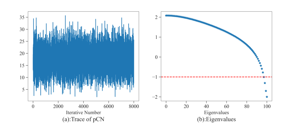
Figure 1: (a): The trace plot of pCN method under the same mesh size of $100$; (b): Logarithm of the eigenvalues $\{c_{k}\}^{n}_{k=1}$ of prior measure. The horizontal red dashed line shows the corresponding eigenvalue $c_{M}$ satisfying $c_{M}/c_{1}<10^{-3}$.

From Theorem 2.9, the stochastic gradient used in the SGD update is

$$\nabla\tilde{\mathcal{L}}(u)=\tilde{\mathcal{G}}_{S}(u)=A(u-\bar{u})-\frac{1}{\sqrt{S}}\xi,$$

where $\xi$ is a mean-zero Gaussian error term in $\mathcal{H}_{u}$ with covariance operator $\mathcal{C}_{\text{noise}}=\mathcal{C}_{0}\mathcal{Q}$. Since random variable $\xi$ is centered, the expected value of $\tilde{\mathcal{G}}_{S}(u)$ is $A(u-\bar{u})$, which equals to $\mathbb{E}[\nabla\tilde{\mathcal{L}}(u)]=A(u-\bar{u})$.

We now characterize the covariance operator of $\operatorname{Cov}(\nabla\tilde{\mathcal{L}}(u))$, which is:

$$\operatorname{Cov}(\nabla\tilde{\mathcal{L}}(u))=\frac{1}{\sqrt{S}}\mathcal{C}_{0}\mathcal{Q}.$$

Then eigenvalues $\{\phi_{i}\}^{M}_{i=1}$ of $\operatorname{Cov}(\nabla\tilde{\mathcal{L}}(u))$ satisfy

$$\operatorname{Cov}(\nabla\tilde{\mathcal{L}}(u))e_{i}=\phi_{i}e_{i}=\frac{1}{S}c_{i}q_{i}e_{i},$$

indicating

$$\phi_{i}=\frac{1}{S}c_{i}q_{i}.$$

That is, by calculate the eigenvalues of covariance $\operatorname{Cov}(\nabla\tilde{\mathcal{L}}(u))$, the eigenvalues $\{q_{i}\}^{M}_{i=1}$ of operator $\mathcal{Q}$ is then calculated by

$$\mathcal{Q}=\sum^{M}_{i=1}q_{i}e_{i}\otimes e_{i}=\sum^{M}_{i=1}\frac{S\phi_{i}}{c_{i}}e_{i}\otimes e_{i}.$$

Substituting $\{q_{i}\}^{M}_{i=1}$ into the bounds for $S$ in Eqs. (2.31) and (2.39), we obtain

• for the cSGD-iVI case, we derive

  $$S<\sqrt{\frac{M^{\prime}}{\sum^{M}_{i=1}\frac{\bm{a}_{\text{max}}\bm{a}_{i}-\bm{a}^{2}_{i}}{q_{i}}}}=\sqrt{\frac{M^{\prime}}{\sum^{M}_{i=1}\frac{\bm{a}_{\text{max}}\bm{a}_{i}-\bm{a}^{2}_{i}}{\frac{S\phi_{i}}{c_{i}}}}}=\sqrt{S\frac{M^{\prime}}{\sum^{M}_{i=1}\frac{\bm{a}_{\text{max}}c_{i}\bm{a}_{i}-c_{i}\bm{a}^{2}_{i}}{\phi_{i}}}}.$$

  That is

  $$S<\frac{M^{\prime}}{\sum^{M}_{i=1}\frac{\bm{a}_{\text{max}}c_{i}\bm{a}_{i}-c_{i}\bm{a}^{2}_{i}}{\phi_{i}}},$$

  where $M^{\prime}=M+\sum_{i=1}^{M}a_{i}c_{i}$, and $\bm{a}_{i}=a_{i}+\frac{1}{c_{i}}$.

• for the pcSGD-iVI case, we derive

  $$S<\sqrt{\frac{M^{\prime}}{\sum^{M}_{i=1}\bigg{(}\frac{\tau_{\text{max}}\bm{a}_{i}}{t_{i}\frac{S\phi_{i}}{c_{i}}}-\frac{\bm{a}^{2}_{i}}{\frac{S\phi_{i}}{c_{i}}}\bigg{)}}}=\sqrt{\frac{M^{\prime}}{\frac{1}{S}\sum^{M}_{i=1}\bigg{(}\frac{\tau_{\text{max}}c_{i}\bm{a}_{i}}{t_{i}\phi_{i}}-\frac{c_{i}\bm{a}^{2}_{i}}{\phi_{i}}\bigg{)}}}.$$

  That is

  $$S<\frac{M^{\prime}}{\sum^{M}_{i=1}\bigg{(}\frac{\tau_{\text{max}}c_{i}\bm{a}_{i}}{t_{i}\phi_{i}}-\frac{c_{i}\bm{a}^{2}_{i}}{\phi_{i}}\bigg{)}},$$

  where $M^{\prime}=M+\sum_{i=1}^{M}a_{i}c_{i}$, and $\bm{a}_{i}=a_{i}+\frac{1}{c_{i}}$.

This completes the specification of $\mathcal{Q}$ through observable quantities $\{q_{i},\phi_{i}\}_{i=1}^{M}$, allowing evaluation of scale bounds for both cSGD-iVI and pcSGD-iVI.

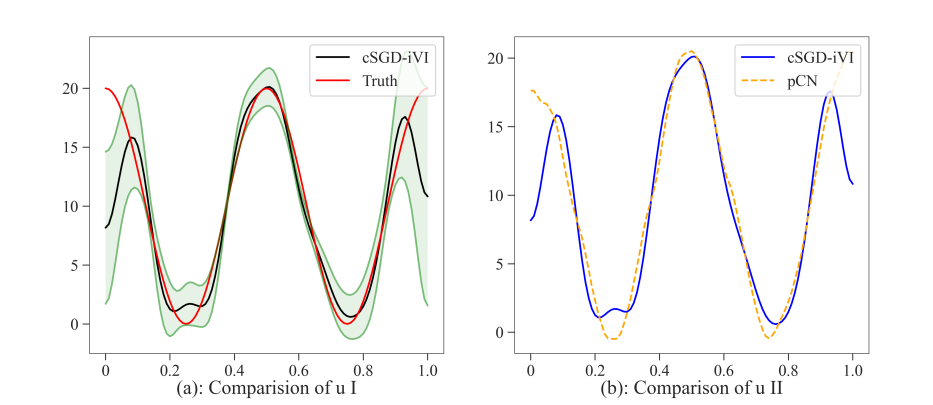
Figure 2: (a): The comparison of the estimated posterior mean function obtained by cSGD-iVI and the background truth of $u$, respectively, and minibatch size $S=10$. The greed shade area represents the $95\%$ credibility region of estimated posterior mean function; (b): The comparison of the estimated posterior mean function obtained by cSGD-iVI and pCN sampling of $u$, respectively, and minibatch size $S=10$.

3 Numerical experiments

We now employ the cSGD-iVI (proposed in 2.2) and pcSGD-iVI (proposed in 2.3) methods to solve two inverse problems, including one linear and one nonlinear case. In Subsection 3.1, we consider a simple smooth model with Gaussian noise; meanwhile, we compare the computational results with those obtained using classical sampling methods, such as the pCN method. Due to space limitations, the nonlinear inverse problem governed by the Darcy flow equation is provided in Section B of the supplementary material.

3.1 The simple elliptic equation with Gaussian noise

3.1.1 Basic settings

Consider an inverse source problem of the elliptic equation

$$\begin{split}-\alpha\Delta w+w&=u\quad\text{in}\ \Omega,\\ w&=0\quad\text{on}\ \partial\Omega,\end{split}$$ (3.1)

where $\Omega=(0,1)\subset\mathbb{R}$, $\alpha>0$ is a positive constant. The forward operator is defined as follows:

$$Hu=(w(x_{1}),w(x_{2}),\cdots,w(x_{N_{d}}))^{T},$$ (3.2)

where $u\in\mathcal{H}_{u}\mathrel{\mathop{\ordinarycolon}}=L^{2}(\Omega)$, $w$ denotes the solution of $(\ref{prob1})$, and $x_{i}\in\Omega$ for $i=1,\cdots,N_{d}$. With these notations, the problem is written abstractly as:

$$\bm{d}=Hu+\bm{\epsilon},$$ (3.3)

where $\bm{\epsilon}\sim\mathcal{N}(0,\bm{\Gamma}_{\text{noise}})$ is the random Gaussian noise. In our implementations, the measurement points $\{x_{i}\}^{N_{d}}_{i=1}$ are taken at the coordinates $\{i/20\}^{20}_{i=1}$. To avoid the inverse crime [23], we discretize the elliptic equation by the finite element method on a regular mesh (the grid points are uniformly distributed on the domain $\Omega$) with the number of grid points being equal to $10^{4}$. In our experiments, the prior measure of $u$ is a Gaussian probability measure $\mu_{0}$ with mean zero and covariance $\mathcal{C}_{0}$.

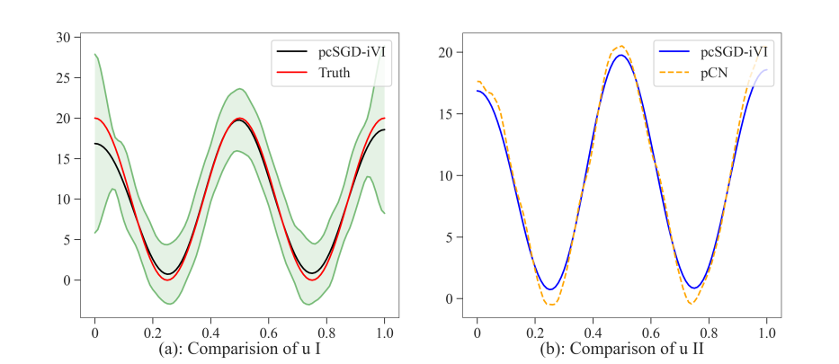
Figure 3: (a): The comparison of the estimated posterior mean function obtained by pcSGD-iVI and the background truth of $u$, respectively, and minibatch size $S=10$. The greed shade area represents the $95\%$ credibility region of estimated posterior mean function; (b): The comparison of the estimated posterior mean function obtained by pcSGD-iVI and pCN of $u$, respectively, and minibatch size $S=10$.

For clarity, we list the specific choices for some parameters introduced in this subsection as follows:

• Assume that 5$\%$ random Gaussian noise $\epsilon\sim\mathcal{N}(0,\bm{\Gamma}_{\text{noise}})$ is added, where $\bm{\Gamma}_{\text{noise}}=\tau^{-1}\textbf{I}$, and $\tau^{-1}=(0.05\max(\lvert Hu\rvert))^{2}$.

• Let domain $\Omega$ be an interval $(0,1)$ with $\partial\Omega=\{0,1\}$. And the available data are assumed to be $\{w(x_{i})|i=1,2,\cdots,20\}$.

• We assume that the data produced from the underlying true signal $u^{\dagger}(x)=10\cdot(\cos 4\pi x+1)$.

• The prior measure of $u$ is given by $\mu_{0}=\mathcal{N}(0,\mathcal{C}_{0})$, where $\mathcal{C}_{0}$ is given by $\mathcal{C}_{0}=(\text{I}-\alpha\Delta)^{-2},$ where $\alpha=0.05$ is a fixed constant. Here the Laplace operator is defined on $\Omega$ with zero Neumann boundary condition.

• In order to avoid inverse crime [23], the data is generated on a fine mesh with the number of grid points equal to $10^{4}$. And we use different sizes of mesh $n=100$ in the inverse stage.

To illustrate the sampling effectiveness of cSGD-iVI and pcSGD-iVI, we compare them to pCN method, which is wildly studied in [8, 12, 30].

3.1.2 Numerical results

In this subsection, we compare the computational results of cSGD-iVI, pcSGD-iVI and pCN methods. Since the covariance operator of the stochastic gradient noise needs to be carefully handled, we follow Subsection 2.4 to compute the operator $\mathcal{Q}$. Based on the formulations of cSGD-iVI and pcSGD-iVI, we adopt different assumptions as described in Subsection C.1 of supplementary material. Here, we briefly discuss the computational cost of the methods considered in this subsection.

Table 1: The relative errors between the covariance matrix, variance function, and covariance functions derived by cSGD-iVI and pCN methods.

Function	$\bm{c}$	$\{c(x_{i},x_{i})\}^{n}_{i=1}$	$\{c(x_{i},x_{i+10})\}^{n-10}_{i=1}$	$\{c(x_{i},x_{i+20})\}^{n-20}_{i=1}$
Relative Error	$2.3057$	$0.2586$	$1.6433$	$10.2072$

Table 2: The relative errors between the covariance matrix, variance function, and covariance functions derived by pcSGD-iVI and pCN method.

Function	$\bm{c}$	$\{c(x_{i},x_{i})\}^{n}_{i=1}$	$\{c(x_{i},x_{i+10})\}^{n-10}_{i=1}$	$\{c(x_{i},x_{i+20})\}^{n-20}_{i=1}$
Relative Error	$0.1703$	$0.05616$	$0.1554$	$0.8971$

First of all, the computational cost of the sampling method is high. In [13, 22], the number of iterations for the sampling method is set to $2\times 10^{5}$ and $4\times 10^{6}$, respectively. To ensure the computational accuracy, we generate $5\times 10^{5}$ samples for the parameter $u$ in this article. Our focus is on the trace of the pCN method, as shown in sub-figure (a) of Figure 1. We see that the whole sampling procedure completely explores the entire sample space. And in sub-figure (b) of Figure 1, we plot the logarithm of the eigenvalues $\{c_{k}\}^{n}_{k=1}$ of the prior measure $\mu_{0}$. The horizontal red dashed line denotes the corresponding eigenvalue $c_{M}$ satisfying $\frac{c_{M}}{c_{1}}<C_{M}=10^{-3}$, where the truncated number $M=97$.

Secondly, let us discuss cSGD-iVI method. For calculating the gradient term in each iteration step, we need to solve one adjoint PDE (corresponding to computing $H^{*}$), and one forward PDE (corresponding to computing $H$). Then each iteration we need to calculate $2$ PDEs. Based on Algorithm 1, the total iteration number is $M*J$, where $M$ is the number of samples, and $J$ is the number of averaging steps per sample. In sub-figure (a) of Figure 4 , we see that the relative errors between samples and background truth becomes small, and the convergence slows down at $60$ step. Hence we set $M=100$ and $J=20$. In summary, it is required to calculate $2MJ$ (each step to calculate gradient of $u$) $=4000$ PDEs during the procedure.

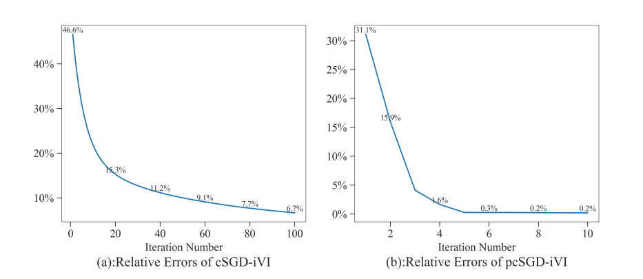
Figure 4: (a): Relative errors of estimated posterior means of $u$ in the $L^{2}-norm$ of cSGD-iVI method with size of mesh $n=100$ and minibatch size $S=10$; (b): Relative errors of estimated posterior means of $u$ in the $L^{2}-norm$ of pcSGD-iVI method with size of mesh $n=100$ and minibatch size $S=10$.

At last, let us discuss pcSGD-iVI method. At each step, we need to compute $T\mathcal{G}(u_{k})$, where $2$ PDEs are required to calculate $\mathcal{G}(u_{k})$, and $2N_{\text{ite}}$ PDEs to solve $T\mathcal{G}(u_{k})$ for accuracy. We currently choose $N_{\text{ite}}$ as $10$. Thus it is required to calculate $2+2N_{\text{ite}}=22$ PDEs in each iteration step. In sub-figure (b) of Figure 4, we see that the relative errors between samples and background truth start to converge at $3$ step, and the descending speed slows down. Hence we choose $M=15$ and $J=20$. In summary, it is required to calculate $22MJ$ (each step to calculate gradient of $u$) $=6600$PDEs during the procedure.

As a result, we need to calculate at most $4000$ PDEs for employing cSGD-iVI method, while $6600$ PDEs for employing pcSGD-iVI method. On the other hand, for the pCN method, $5\times 10^{5}$ PDEs are needed to be calculated. We conclude that the computational cost of these two methods are much less than the cost of pCN method.

Next, we illustrate the numerical results obtained by both methods, and compare them to the results of pCN. As [12] shows, pCN method provides a good estimate of the posterior measure of $u$. It is necessary for us to compare the estimated posterior measures of $u$ obtined by these three methods. Then we provide some discussions about the estimated posterior mean and covariance functions.

Let us provide some discussions of estimated posterior mean function. As shown in sub-figure (a) of Figure 2, the mean function of estimated posterior measure of $u$ obtained by the cSGD-iVI method and the background truth are drawn in black solid and red solid lines, respectively. Two green lines represent the upper and lower bounds of the $95\%$ credibility region of the estimated posterior mean function. We see that the $95\%$ credibility region includes the background truth in most of the region of $u$; however on the left part, credibility region does not. This illustrates that the estimated posterior measure derived by cSGD-iVI could not fully reflect the uncertainty of $u$ completely. In sub-figure (a) of Figure 3, the mean function of estimated posterior measure of $u$ obtained by the pcSGD-iVI method and the background truth are drawn in black solid and red solid lines, respectively. The $95\%$ credibility region includes the background truth, which means the estimated posterior measure obtained by pcSGD-iVI reflects the uncertainty of $u$.

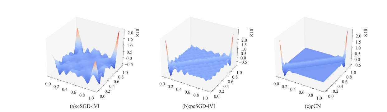
Figure 5: The comparison of estimated posterior covariance operators of $u$ with mesh size $n=100$, minibatch size $S=10$, respectively. (a): The covariance operator obtained by cSGD-iVI method; (b): The covariance operator obtained by pcSGD-iVI method; (c): The covariance operator obtained by pCN method.

In Figure 4, we show the relative errors of both methods, which is defined by

$$\text{relative error}=\frac{\lVert u_{k,J}-u^{\dagger}\rVert^{2}_{2}}{\lVert u^{\dagger}\rVert^{2}_{2}},$$ (3.4)

where $J$ is the averaging converging steps defined in Algorithms 1 and 2. As shown in sub-figure (a) of Figure 4, the relative error curve illustrates that the iteration process of cSGD-iVI converges within $100$ steps, and is stable around $7\%$ at the end of the iteration. The convergence speed is fast since the descending trend is rapid at first $20$ steps. As shown in sub-figure (b) of Figure 4, the relative error curve illustrates that the iteration process of pcSGD-iVI converges within $10$ steps, and is stable around $0.2\%$ at the end of the iteration. Based on the visual (sub-figure (a) of Figures 2 and 3) and quantitative (relative errors shown in Figure 4) evidence, we conclude that the pcSGD-iVI method provides estimated posterior mean functions for the parameter $u$ that closely match the background truth; ; however, the cSGD-iVI mean function is less accurate near the left and right boundaries compared to pcSGD-iVI.

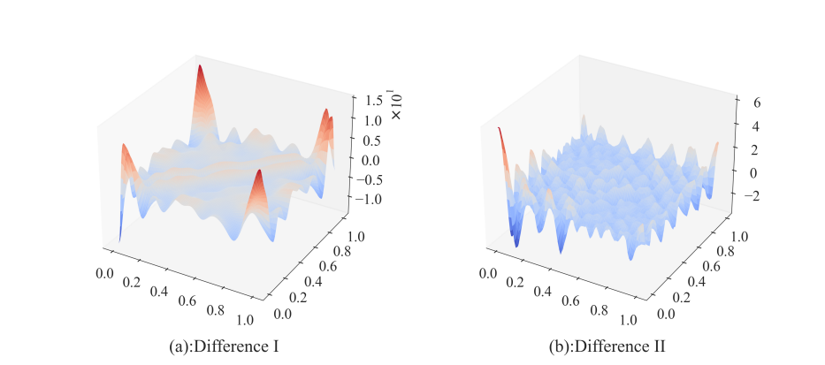
Figure 6: (a): The difference of covariance operator, obtained by cSGD-iVI and pCN methods; (b): The difference of covariance operator, obtained by pcSGD-iVI and pCN methods.

Furthermore, we provide numerical evidence to support a comparison of the estimated posterior mean functions obtained by both methods with the pCN method. The comparison of estimated posterior mean functions obtained by cSGD-iVI (blue solid line) and pCN (orange dashed line) is drawn in sub-figure (b) of Figure 2. The differences are visually small in the middle region but become larger near the left, right, and corner areas. The relative error between them is given by

$$\text{relative error}\mathrel{\mathop{\ordinarycolon}}=\frac{\lVert u^{*}_{\text{cSGD}}-u^{*}_{\text{pCN}}\rVert^{2}_{L^{2}}}{\lVert u^{*}_{\text{pCN}}\rVert^{2}_{L^{2}}}=0.04755.$$ (3.5)

On the other hand, the comparison of pcSGD-iVI (blue solid line) and pCN (orange dashed line) is drawn in sub-figure (b) of Figure 3. The differences are also small in the central, left, and right parts of the domain but slightly more pronounced in the corners. The relative error between them is given by

$$\text{relative error}\mathrel{\mathop{\ordinarycolon}}=\frac{\lVert u^{*}_{\text{cSGD}}-u^{*}_{\text{pCN}}\rVert^{2}_{L^{2}}}{\lVert u^{*}_{\text{pCN}}\rVert^{2}_{L^{2}}}=0.005031.$$ (3.6)

Hence, the estimated posterior mean function derived by pcSGD-iVI are quantitatively similar to that by pCN method; however the estimated posterior mean obtained from cSGD-iVI is worse. As a result, combining visual (sub-figure (b) of Figures 2 and 3) and quantitative (relative errors given in (3.5) and (3.6)) evidence, we conclude that pcSGD-iVI provides a better estimate of the posterior mean function than the cSGD-iVI method.

Next, we provide some discussions of estimated posterior covariance functions. For the numerical convenience, we compare the estimated posterior covariance matrices, variances, and covariance functions The definitions and notations of covariance matrix, variance function and covariance function of the posterior covariance are provided in Subsection C.2 of supplementary material.

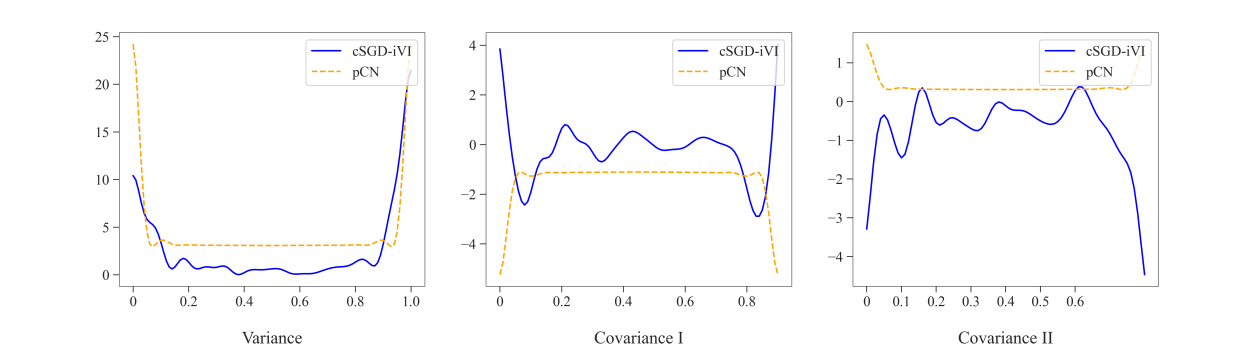
Figure 7: Comparison of variance, covariance functions obtained by cSGD-iVI and pCN methods. (a): The variance function $\{c(x_{i},x_{i})\}^{100}_{i=1}$ on all the mesh point pairs $\{(x_{i},x_{i})\}^{100}_{i=1}$; (b): The covariance function $\{c(x_{i},x_{i+10})\}^{90}_{i=1}$ on the mesh points $\{(x_{i},x_{i+10})\}^{90}_{i=1}$; (c): The covariance function $\{c(x_{i},x_{i+20})\}^{80}_{i=1}$ on the mesh points $\{(x_{i},x_{i+20})\}^{80}_{i=1}$.

In Tables 1 and 2, we compare the variance, covariance functions of cSGD-iVI and pCN methods, pcSGD-iVI and pCN methods, respectively. We see that the relative errors shown in Table 1 are larger than that shown in Table 2. In both tables, the relative errors for the variance functions are significantly smaller than those for the covariance functions. For pcSGD-iVI, the covariance matrices, variance functions, and covariance functions are quantitatively similar to those produced by the pCN method. Conversely, the covariance matrices, variances, and covariance functions derived by cSGD-iVI differ more notably from those obtained by pCN, particularly in the covariance functions. Quantitatively, this suggests that pcSGD-iVI yields a closer approximation to the posterior covariance operator than cSGD-iVI.

In Figure 5, we draw the covariance matrix $\bm{c}_{\text{cSGD}}$, $\bm{c}_{\text{pcSGD}}$, and $\bm{c}_{\text{pCN}}$ in the sub-figures (a), (b), and (c). In Figure 6, we draw the differences between $\bm{c}_{\text{cSGD}}$ and $\bm{c}_{\text{pCN}}$ in sub-figure (a); the differences between $\bm{c}_{\text{pcSGD}}$ and $\bm{c}_{\text{pCN}}$ in sub-figure (b), respectively. Combining Figures 5 and 6, we see that the covariance operator obtained by pcSGD-iVI is more similar to that of the pCN method, and the differences are visually small; whereas the covariance operator derived from cSGD-iVI deviates more significantly. Furthermore, we provide a detailed comparison of the variance and covariance functions obtained by these three method in Figures 7 and 8, respectively. In all the sub-figures of Figures 7 and 8, the variance and covariance functions obtained by both iVI methods are shown in blue solid lines, while those from pCN are plotted in orange dashed lines. In sub-figures (a) of Figures 7 and 8, we show the variance function calculated on all the mesh point pairs $\{(x_{i},x_{i})\}^{n}_{i=1}$ with $n=100$. In sub-figures (b) and (c), we show the covariance functions calculated on the pairs of points $\{(x_{i},x_{i+10})\}^{n-10}_{i=1}$, and $\{(x_{i},x_{i+20})\}^{n-20}_{i=1}$, respectively.

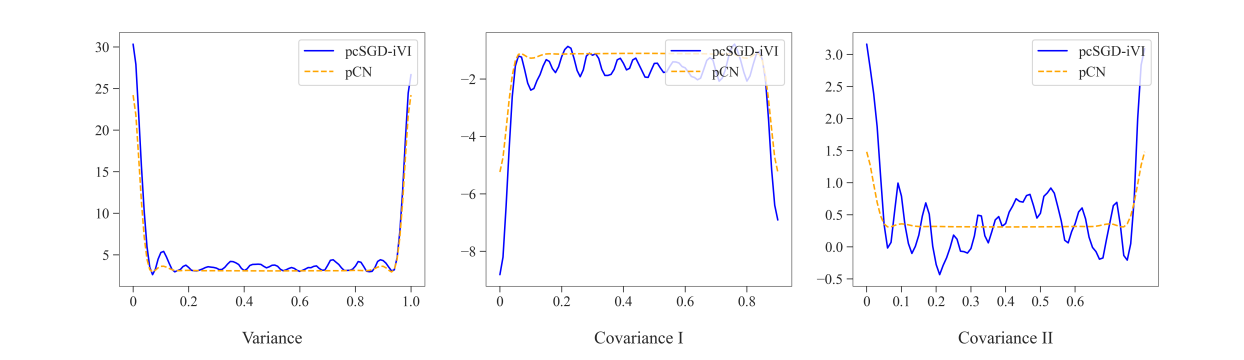
Figure 8: Comparison of variance, covariance functions obtained by pcSGD-iVI and pCN methods. (a): The variance function $\{c(x_{i},x_{i})\}^{100}_{i=1}$ on all the mesh point pairs $\{(x_{i},x_{i})\}^{100}_{i=1}$; (b): The covariance function $\{c(x_{i},x_{i+10})\}^{90}_{i=1}$ on the mesh points $\{(x_{i},x_{i+10})\}^{90}_{i=1}$; (c): The covariance function $\{c(x_{i},x_{i+40})\}^{80}_{i=1}$ on the mesh points $\{(x_{i},x_{i+20})\}^{20}_{i=1}$.

The covariance matrices, variance functions, and covariance functions obtained by cSGD-iVI show large deviations from those produced by pCN. In contrast, the differences between pcSGD-iVI and pCN are much smaller. The errors associated with cSGD-iVI are significantly larger than those of pcSGD-iVI. This suggests that the covariance operator of cSGD-iVI diverges considerably from that of pCN, whereas the operator from pcSGD-iVI closely resembles that of pCN, consistent with the visual results. Furthermore, as is seen in the sub-figure (a) of Figure 3, the $95\%$ credibility region of the estimated posterior mean contains the background truth, which indicates that the Bayesian setup derived by pcSGD-iVI is meaningful and in accordance with the frequentist theoretical investigations of the posterior consistency [35, 39]. Overall, we conclude that the pcSGD-iVI method provides a better estimate of the posterior covariance than cSGD-iVI, based on the visual (Figures 5, 6, 7 and 8) and quantitative (Tables 1 and 2) evidence.

Now we provide conclusions about the estimated posterior measures corresponding to parameter $u$ obtained by cSGD-iVI and pcSGD-iVI. In Bayesian inference, an accurate approximation of the posterior distribution requires not only a good estimate of the mean function, but also a reliable estimate of the covariance, which quantifies the uncertainty of parameter $u$. As discussed previously, the posterior mean of $u$ estimated by pcSGD-iVI closely matches that obtained by pCN, based on the visual (sub-figure (b) of Figure 3) and quantitative (relative error calculated in (3.6)) evidence, moreover, $95\%$ credibility region of the estimated mean function includes background truth. But the mean function of cSGD-iVI is worse based on the visual (sub-figure (b) of Figure 2) and quantitative (relative error calculated in (3.5)) evidence, while $95\%$ credibility region of the estimated mean function could not include background truth completely. Based on the visual evidence (Figures 5 and $\ref{fig:Variances_pcSGD})$, the posterior covariance matrices, variance functions, and covariance functions derived from pcSGD-iVI and pCN appear visually similar. And quantitative evidence (Table 2) shows that the relative errors between the covariance matrices, variance, and covariance functions are quantitatively small, which indicates that the posterior covariance obtained by pcSGD-iVI method is as good as that by pCN method. But the covariance operator obtained of cSGD-iVI is much different from that of pCN based on visual evidence (Figures 5 and $\ref{fig:Variances_cSGD})$, and quantitative evidence (Table 1) shows that relative errors are large. These indicates that cSGD-iVI could not provide a reliable estimate of posterior covariance operator. In summary, both visual and quantitative results indicate that pcSGD-iVI provides a more reliable approximation of the posterior mean function and covariance operator than cSGD-iVI.

4 Conclusion

In this paper, we develop cSGD-iVI and pcSGD-iVI methods in infinite-dimensional spaces, extending the finite-dimensional cSGD inference method proposed in [27, 28]. Based on Subsection 2.2, we reformulate the cSGD method within a Bayesian inference framework. By solving the inference problem, we identify an optimal learning rate that minimizes the KL divergence between the estimated and true posterior measures, enabling sampling from the estimated posterior via the cSGD iteration. We further introduce the pcSGD-iVI method, which builds upon the cSGD-iVI framework. We propose a learning rate that minimizes the KL divergence between the estimated and true posterior measures. Additionally, by treating the stochastic gradient as a random variable, we derive its corresponding probability distribution and thereby introduce the prior operator $\mathcal{Q}$. We also establish the regularization properties of the cSGD formulation and provide discretization error bounds between the estimated posterior mean, posterior samples, and the truth function, which depend on the learning rate and discretization level. The proposed cSGD-iVI and pcSGD-iVI methods are applied to two inverse problems: a simple elliptic problem and a steady-state Darcy flow problem. For both cases, the pcSGD-iVI method yields estimated posterior measures for the parameter $u$ that closely resemble the true posterior, accurately reflecting the uncertainty in $u$, as supported by both visual and quantitative evidence. In contrast, the cSGD-iVI method produces less accurate posterior mean functions and covariance operators, especially in the Darcy flow problem.

Our current implementations of cSGD-iVI and pcSGD-iVI are based on linear inverse problems. For nonlinear problems, these methods can only address linearized formulations and produce approximate posterior measures. As a result, the estimated posterior may not be sufficiently accurate for highly nonlinear inverse problems.

References

- [1] Wolfgang Arendt, Isabelle Chalendar, and Robert Eymard, Galerkin approximation of linear problems in banach and hilbert spaces, IMA Journal of Numerical Analysis 42 (2020), no. 1, 165–198.
- [2] Simon Arridge, Peter Maass, Ozan Öktem, and Carola-Bibiane Schönlieb, Solving inverse problems using data-driven models, Acta Numerica 28 (2019), 1–174.
- [3] Alexandros Beskos, Mark Girolami, Shiwei Lan, Patrick E. Farrell, and Andrew M. Stuart, Geometric MCMC for infinite-dimensional inverse problems, Journal of Computational Physics 335 (2017), 327–351.
- [4] David M. Blei, Alp Kucukelbir, and Jon D. McAuliffe, Variational inference: A review for statisticians, Journal of the American Statistical Association 112 (2017), no. 518, 859–877.
- [5] Tan Bui-Thanh, Omar Ghattas, James Martin, and Georg Stadler, A computational framework for infinite-dimensional Bayesian inverse problems Part I: The linearized case, with application to global seismic inversion, SIAM Journal on Scientific Computing 35 (2013), no. 6, A2494–A2523.
- [6] Tan Bui-Thanh and Quoc P. Nguyen, FEM-based discretization-invariant MCMC methods for PDE-constrained Bayesian inverse problems, Inverse Problems & Imaging 10 (2016), no. 4, 943–975.
- [7] Simon L. Cotter, Massoumeh Dashti, James C. Robinson, and Andrew M. Stuart, Bayesian inverse problems for functions and applications to fluid mechanics, Inverse Problems 25 (2009), no. 11, 115008.
- [8] Simon L. Cotter, Gareth O. Roberts, Andrew M. Stuart, and David White, MCMC methods for functions: Modifying old algorithms to make them faster, Statistical Science 28 (2013), no. 3, 424–446.
- [9] Tiangang Cui, Martin James, M. Marzouk Youssef, Solonen Antti, and Alessio Spantini, Likelihood-informed dimension reduction for nonlinear inverse problems, Inverse Problems 30 (2014), no. 11, 114015.
- [10] Tiangang Cui, Youssef Marzouk, and Karen Willcox, Scalable posterior approximations for large-scale bayesian inverse problems via likelihood-informed parameter and state reduction, Journal of Computational Physics 315 (2016), 363–387.
- [11] Tiangang Cui and Olivier Zahm, Data-free likelihood-informed dimension reduction of bayesian inverse problems, Inverse Problems 37 (2021), no. 4, 045009.
- [12] Masoumeh Dashti and Andrew M. Stuart, The Bayesian Approach to Inverse Problems, Handbook of uncertainty quantification, Springer, 2017, pp. 311–428.
- [13] Matthew M. Dunlop, Marco A. Iglesias, and Andrew M. Stuart, Hierarchical Bayesian level set inversion, Statistics and Computing 27 (2017), no. 6, 1555–1584.
- [14] Zhe Feng and Jinglai Li, An adaptive independence sampler MCMC algorithm for Bayesian inferences of functions, SIAM Journal on Scientific Computing 40 (2018), no. 3, A1301–A1321.
- [15] Andreas Fichtner, Full Seismic Waveform Modelling and Inversion, Springer, Heidelberg, 2010.
- [16] Nilabja Guha, Xiaoqing Wu, Yalchin Efendiev, Bangti Jin, and Bani K. Mallick, A variational Bayesian approach for inverse problems with skew-t error distribution, Journal of Computational Physics 301 (2015), 377–393.
- [17] Michael Hinze, René Pinnau, Michael Ulbrich, and Stefan Ulbrich, Optimization with PDE Constraints, Springer, New York, 2008.
- [18] Zixi Hu, Zhewei Yao, and Jinglai Li, On an adaptive preconditioned Crank-Nicolson MCMC algorithm for infinite dimensional Bayesian inferences, Journal of Computational Physics 332 (2017), 492–503.
- [19] Junxiong Jia, Peijun Li, and Deyu Meng, Stein variational gradient descent on infinite-dimensional space and applications to statistical inverse problems, SIAM Journal on Numerical Analysis 60 (2022), no. 4, 2225–2252.
- [20] Junxiong Jia, Yanni Wu, Peijun Li, and Deyu Meng, Variational inverting network for statistical inverse problems of partial differential equations, arXiv:2201.00498 (2022), 1–46.
- [21] Junxiong Jia, Qian Zhao, Zongben Xu, Deyu Meng, and Yee Leung, Variational Bayes’ method for functions with applications to some inverse problems, SIAM Journal on Scientific Computing 43 (2021), no. 1, A355–A383.
- [22] Bangti Jin and Jun Zou, Hierarchical Bayesian inference for ill-posed problems via variational method, Journal of Computational Physics 229 (2010), no. 19, 7317–7343.
- [23] Jari Kaipio and Erkki Somersalo, Statistical and Computational Inverse Problems, Springer-Verlag, New York, 2005.
- [24] Bartek T. Knapik, Aad W. Van Der Vaart, and J. Harry van Zanten, Bayesian inverse problems with gaussian priors, The Annals of Statistics 39 (2011), no. 5, 2626–2657.
- [25] Matti Lassas and Samuli Siltanen, Can one use total variation prior for edge-preserving Bayesian inversion?, Inverse Problems 20 (2004), no. 5, 1537–1563.
- [26] Shuai Lu and Peter Mathé, Stochastic gradient descent for linear inverse problems in Hilbert spaces, Mathematics of Computation 91 (2022), no. 336, 1763–1788.
- [27] Stephan Mandt, Matthew D. Hoffman, and David M. Blei, A variational analysis of stochastic gradient algorithms, Proceedings of The 33rd International Conference on Machine Learning 48 (2016), 354–363.
- [28] , Stochastic gradient descent as approximate bayesian inference, Journal of Machine Learning Research 18 (2017), no. 134, 1–35.
- [29] Peter Mathé and Sergei V Pereverzev, Discretization strategy for linear ill-posed problems in variable Hilbert scales, Inverse Problems 19 (2003), no. 6, 1263.
- [30] Natesh S. Pillai, Andrew M. Stuart, and Alexandre H. Thiéry, Noisy gradient flow from a random walk in Hilbert space, Stochastic Partial Differential Equations: Analysis and Computations 2 (2014), no. 2, 196–232.
- [31] Frank J. Pinski, Gideon Simpson, Andrew M. Stuart, and Hendrik Weber, Algorithms for Kullback–Leibler approximation of probability measures in infinite dimensions, SIAM Journal on Scientific Computing 37 (2015), no. 6, A2733–A2757.
- [32] Frank J Pinski, Gideon Simpson, Andrew M. Stuart, and Hendrik Weber, Kullback-Leibler approximation for probability measures on infinite dimensional space, SIAM Journal on Mathematical Analysis 47 (2015), no. 6, 4091–4122.
- [33] Andrew M. Stuart, Inverse problems: A Bayesian perspective, Acta Numerica 19 (2010), 451–559.
- [34] Jiaming Sui and Junxiong Jia, Non-centered parametric variational Bayes’ approach for hierarchical inverse problems of partial differential equations, Mathematics of Computation 93 (2024), no. 348, 1715–1760.
- [35] Yixin Wang and David M Blei, Frequentist consistency of variational Bayes, Journal of the American Statistical Association 114 (2019), no. 527, 1147–1161.
- [36] Arthur B. Weglein, Fernanda V. Araújo, Paulo M. Carvalho, Robert H. Stolt, Kenneth H. Matson, Richard T. Coates, Dennis Corrigan, Douglas J. Foster, Simon A. Shaw, and Haiyan Zhang, Inverse scattering series and seismic exploration, Inverse Problems 19 (2003), no. 6, R27–R83.
- [37] Zhewei Yao, Zixi Hu, and Jinglai Li, A TV-gaussian prior for infinite-dimensional Bayesian inverse problems and its numerical implementations, Inverse Problems 32 (2016), 075006–1.
- [38] Cheng Zhang, Judith Bütepage, Hedvig Kjellström, and Stephan Mandt, Advances in variational inference, IEEE Transactions on Pattern Analysis and Machine Intelligence 41 (2018), no. 8, 2008–2026.
- [39] Fengshuo Zhang and Chao Gao, Convergence rates of variational posterior distributions, The Annals of Statistics 48 (2020), no. 4, 2180–2207.
- [40] Qingping Zhou, Zixi Hu, Zhewei Yao, and Jinglai Li, A hybrid adaptive MCMC algorithm in function spaces, SIAM/ASA Journal on Uncertainty Quantification 5 (2017), no. 1, 621–639.
- [41] Qingping Zhou, Tengchao Yu, Xiaoqun Zhang, and Jinglai Li, Bayesian inference and uncertainty quantification for medical image reconstruction with Poisson data, SIAM Journal on Imaging Sciences 13 (2020), no. 1, 29–52.