Composite Optimization with Indicator Functions:
Stationary Duality and a Semismooth Newton Method

Abstract

Indicator functions of taking values of zero or one are essential to numerous applications in machine learning and statistics. The corresponding primal optimization model has been researched in several recent works. However, its dual problem is a more challenging topic that has not been well addressed. One possible reason is that the Fenchel conjugate of any indicator function is finite only at the origin. This work aims to explore the dual optimization for the sum of a strongly convex function and a composite term with indicator functions on positive intervals. For the first time, a dual problem is constructed by extending the classic conjugate subgradient property to the indicator function. This extension further helps us establish the equivalence between the primal and dual solutions. The dual problem turns out to be a sparse optimization with a $\ell_{0}$ regularizer and a nonnegative constraint. The proximal operator of the sparse regularizer is used to identify a dual subspace to implement gradient and/or semismooth Newton iteration with low computational complexity. This gives rise to a dual Newton-type method with both global convergence and local superlinear (or quadratic) convergence rate under mild conditions. Finally, when applied to AUC maximization and sparse multi-label classification, our dual Newton method demonstrates satisfactory performance on computational speed and accuracy.

Keywords: Composite optimization Indicator function Dual stationarity Semismooth Newton method Global convergence Local superlinear convergence rate

1 Introduction

In this work, we aim to solve the following nonconvex composite optimization

$$\min_{{\bf x}\in{\mathbb{R}}^{n}}f({\bf x})+\bm{\mathcal{I}}(A{\bf x}+{\bf b}),$$ (1)

where $f:\mathbb{R}^{n}\to{\mathbb{R}}$ is a $\sigma_{f}$-strongly convex function (possibly nonsmooth), and $A\in{\mathbb{R}}^{m\times n}$ and ${\bf b}\in{\mathbb{R}}^{m}$ are given data. For ${\bf u}=(u_{1},\cdots,u_{m})^{\top}$, we define $\bm{\mathcal{I}}({\bf u})=\lambda\sum_{i=1}^{m}{\bf 1}_{(0,\infty)}(u_{i})$, where $\lambda$ is a positive constant and ${\bf 1}_{(0,\infty)}$ is the indicator function on the positive interval (also called zero-one loss), defined as

$${\bf 1}_{(0,\infty)}(t)=\left\{\begin{aligned} &1,\quad\mbox{ if }t>0,\\ &0,\quad\mbox{ if }t\leq 0.\end{aligned}\right.$$

Problem (1) arises from extensive applications, including multi-label classification [66], area under the receiver operating characteristic curve (AUC) [23, 28], maximum ranking correlation [26, 33], to mention a few. The strongly convex function $f$ often serves as a regularizer in these tasks, including squared $\ell_{2}$ norm for margin maximization (e.g. [18, 59]) or (group) elastic net for feature selection (e.g. [71, 48, 63]). Problem (1), in particular, covers the composite $\ell_{0}$-norm: $\|B{\bf x}+{\bf b}\|_{0}=\bm{\mathcal{I}}(B{\bf x}+{\bf b})+\bm{\mathcal{I}}(-B{\bf x}-{\bf b}).$ The matrix $A$ becomes $[B;-B]$ (Matlab notation) and this implies that the rows of $A$ are dependent. Therefore, it is essential we do not assume that $A$ has a full-row rank property. And we do not assume that $f$ is smooth.

When $f$ is smooth, several progresses have been made in solving the primal nonconvex composition problem involving the indicator function or a lower semi-continuous (l.s.c) function. These methods include, but are not limited to the Newton method [70], augmented Lagrangian-based method [10, 11, 38, 61], lifted reformulation [19, 27], and complementarity reformulation [22, 32]. However, the composition of a nonconvex, discontinuous indicator function and a large-scale matrix brings significant difficulty in both convergence and computation. For example, certain regularity conditions (such as a full row-rank matrix $A$) are often required for the convergence analysis of the aforementioned algorithms. Moreover, it still remains a difficult task to globalize a primal Newton method while retaining local quadratic convergence. Finally, we should stress that the function $f$ in (1) is not necessarily smooth. This together with the combinatorial nature of $\bm{\mathcal{I}}$ poses significant barriers to designing a globally convergent algorithm for (1).

This paper offers an alternative methodology, strongly motivated by the classical duality theory of convex optimization. We will propose a dual reformulation of (1) with a conducive structure for numerical computation. In the following, we first explain the motivation that leads to a framework for constructing the dual problem. We then briefly summarize the main contributions of the paper.

1.1 Motivation from convex optimization

Let us recall the Fenchel duality in convex optimization (see [56, Chap. 31] and [4, 14]):

$$\inf_{{\bf x}\in{\mathbb{R}}^{n}}~\Big{\{}f({\bf x})+\varphi(A{\bf x}+{\bf b})\Big{\}}=\sup_{{\bf z}\in{\mathbb{R}}^{m}}\left\{-f^{*}(-A^{\top}{\bf z})+\langle{\bf b},{\bf z}\rangle-\varphi^{*}({\bf z})\right\}.$$ (2)

where both $f$ and $\varphi$ are closed, proper, and convex, and $f^{*}$ and $\varphi^{*}$ are their respective conjugate functions. For simplicity of discussion, we omit the relative interior conditions for the duality to hold. The dual problem is often advantageous to solve due to a few features. Firstly, the matrix $A$ has been separated from the possibly nonsmooth function $\varphi$ while composited with $f^{*}$. Secondly, $f^{*}$ has Lipschitzian continuous gradient when $f$ is strongly convex. Thirdly, in many applications, $\varphi^{*}$ has a closed-form proximal operator that would allow proximal gradient method to be developed, see [4]. An impressive progress has been made on applying the dual approach to LASSO-type problems and highly efficient semismooth Newton algorithms are developed, see [39, 68] and the references therein. Recently, [24] proposed the semismoothness* of a set-valued mapping, which is an improvement of classic semismoothness. For minimization of a prox-regular function, [46] designed a generalized Newton method based on the second-order subdifferential [42] and proved its local superlinear convergence under semismoothness* and tilt stability assumptions. This method is further developed for solving composite optimization [34, 35, 36] and difference programming [1] under some assumptions. A more comprehensive introduction to this method can be found in the monograph [45]. These works motivated us to investigate whether a dual approach is viable for (1) and whether a generalized Newton method can be constructed.

However, if we blindly apply the dual formulation (2) to (1) with $\varphi=\bm{\mathcal{I}}$, we would not gain much. This is because the conjugate function $\bm{\mathcal{I}}^{*}$ only takes finite value at $\{0\}$:

$$\bm{\mathcal{I}}^{*}({\bf z}):=\sup_{{\bf u}\in{\mathbb{R}}^{m}}\Big{\{}\langle{\bf z},{\bf u}\rangle-\bm{\mathcal{I}}({\bf u})\Big{\}}=\left\{\begin{aligned} &0,&&\mbox{if }{\bf z}=0,\\ &\infty,&&\mbox{otherwise}.\end{aligned}\right.$$

This means that the dual problem would have only one feasible point ${\bf z}=0$ and everything we care about in duality breaks down.

Now let us take a step back to recall one essential property for the conjugate function pair $(\varphi,\varphi^{*})$ when $\varphi$ is proper, closed, and convex:

$${\bf z}\in\partial\varphi({\bf u})~~\Longleftrightarrow~~{\bf u}\in\partial\varphi^{*}({\bf z}),$$

where $\partial\varphi(\cdot)$ is the subdifferential of $\varphi(\cdot)$ in convex analysis [56]. We call this property the stationary duality property. We would like to find a function $g(\cdot)$ that plays the role of $\bm{\mathcal{I}}^{*}(\cdot)$ and satisfies the stationary duality property:

$${\bf z}\in\partial\bm{\mathcal{I}}({\bf u})~~\Longleftrightarrow~~{\bf u}\in\partial g({\bf z}),$$ (3)

where $\partial\bm{\mathcal{I}}(\cdot)$ is the limiting subdifferential in variational analysis [44, 57]. In the meantime, we require the function $g({\bf z})$ to inherit some useful information from the primal Problem (1). For the one-dimensional case, the construction of such function $g(z)$ is demonstrated in Fig. 1.

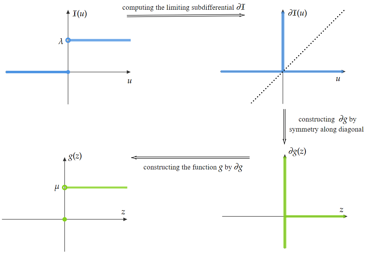
Figure 1: Constructing a function $g$ such that $z\in\partial\bm{\mathcal{I}}(u)$ if and only if $u\in\partial g(z)$ for any given $z,u\in{\mathbb{R}}$.

1.2 Stationary duality and main contributions

Extension of the one-dimensional case to the multi-dimensional case leads to the following function:

$$g({\bf z}):=\mu\|{\bf z}\|_{0}+\bm{\delta}_{+}({\bf z}),$$ (4)

where $\mu>0$ is a parameter and $\bm{\delta}_{+}(\cdot)$ is defined as follows:

$$\bm{\delta}_{+}({\bf z})=\left\{\begin{aligned} &0,&&\mbox{ if }{\bf z}\geq 0,\\ &+\infty,&&\mbox{ otherwise}.\end{aligned}\right.$$

Using the characterizations in (6) and (7), it is easy to verify that the stationary dual relationship (3) holds for $g(\cdot)$. This gives rise to the stationary dual problem:

$$\max_{{\bf z}\in\mathbb{R}^{m}}~-h({\bf z})-g({\bf z})\qquad\mbox{with}\quad h({\bf z}):=f^{*}(-A^{\top}{\bf z})-\langle{\bf z},{\bf b}\rangle.$$ (5)

Although we cannot expect the perfect duality in convex optimization, we are able to establish the following important results.

• There is one-to-one correspondence between local minimizers of the primal problem (1) and that of the dual problem (5). See Thm. 10 for the detailed formula for computing the corresponding solution from the other. This is achieved through the study of proximal-type (“P-” for short) stationary point of (5) and its correspondence to the KKT (Karush-Kuhn-Tucker) point of a local convex reformulation of (1) at a local minimizer. This result is the basis for further numerical development.

• Since $f$ is strongly convex, its conjugate $f^{*}$ has Lipschitzian continuous gradient and well-defined generalized Jacobian. More importantly, the nonsmooth function $g$ is a sparse regularizer with a closed-form proximal operator, which helps us identify a dual subspace to perform low-complexity iteration. In this reduced subspace, we can first implement a gradient step and then accelerate it by a semismooth Newton step. In this process, easy-to-check conditions are proposed to ensure the dual objective function in (5) ascent. These steps form the basic framework of our subspace gradient semismooth Newton (SGSN) method, see Alg. 1.

• In addition to the low per-iteration complexity, our SGSN has global convergence with local superliner (or quadratic) rate. If the generated sequence is bounded and the dual objective function in (5) satisfies Polyak-Łojasiewicz-Kurdyka (PŁK) property, then the sequence converges to a P-stationary point of (5) (Thm. 16). Thereby, a local minimizer of the primal Problem (1) is found. This result does not require the regularity condition that the matrix $A$ has full-row rank. If we further assume that the gradient function $\nabla f^{*}$ is (strongly) semismooth and a second-order sufficient condition holds, then the sequence converges to a P-stationary point of (5) with local superlinear (or quadratic) rate. To the best of our knowledge, SGSN is the first algorithm that enjoys both global convergence and local superlinear rate for Problem (1) (Thm. 19). Finally, we demonstrate the use of SGSN on two important applications: AUC maximization and the sparse multi-label classification. The experiments show that SGSN has satisfactory performance on computational speed and solution accuracy when benchmarking against several competitive algorithms.

1.3 Organization

The paper is organized as follows. Some frequently used symbols and notations are introduced in Section 2. The one-to-one correspondence between solutions of primal and dual problems is established in Section 3. To find a dual solution, we describe the framework of SGSN and prove its global convergence with a local superlinear (or quadratic) rate in Section 4. The numerical experiments on AUC maximization and multi-label classification are conducted in Section 5. We conclude the paper in Section 6 with some discussion on possible future research.

2 Preliminaries

In this part, we first describe the notation used in the paper. We then recall the definition of the limiting subdifferential and apply it to the function $g(\cdot)$ in (4). We also characterize its proximal operator. Finally, we introduce some function classes.

2.1 Notation

The boldfaced lowercase letter ${\bf x}\in\mathbb{R}^{n}$ denotes a column vector of size $n$ and ${\bf x}^{\top}$ is its transpose. Let $x_{i}$ or $[{\bf x}]_{i}$ denote the $i$th element of ${\bf x}$. We let ${\mathbb{R}}^{n}_{+}$ denote the non-negative orthant in $\mathbb{R}^{n}$. The norm $\|\cdot\|$ denotes the $\ell_{2}$ norm of ${\bf x}$ or the Frobenius norm for a matrix $A$, and thus we always have $\|A{\bf x}\|\leq\|A\|\|{\bf x}\|.$ A neighborhood of ${\bf x}^{*}\in\mathbb{R}^{n}$ is often denoted as $\mathcal{N}({\bf x}^{*})$, while $\mathcal{N}({\bf x}^{*},\delta):=\{{\bf x}\in\mathbb{R}^{n}\ |\ \|{\bf x}-{\bf x}^{*}\|<\delta\}$ when the radius $\delta>0$ is given. We denote $I$ as the identity matrix of appropriate dimension. Let ${\bf e}$ represent a vector of all 1’s with dimension implied by the context. We denote ceiling and floor functions as $\lceil\cdot\rceil$ and $\lfloor\cdot\rfloor$ respectively.

Let $[m]$ denote the set of indices $\{1,\ldots,m\}$. For a subset $\Gamma\subset[m]$, ${\overline{\Gamma}}$ consists of those indices of $[m]$ not in $\Gamma$ and $|\Gamma|$ denotes the number of elements in $\Gamma$ (cardinality of $\Gamma$). For vector ${\bf z}\in\mathbb{R}^{m}$ (resp. matrix $A\in{\mathbb{R}}^{m\times n}$), ${\bf z}_{\Gamma}$ (resp. $A_{\Gamma:}$) denotes the subvector of ${\bf z}$ indexed by $\Gamma$ (resp. the submatrix of $A$ with rows indexed by $\Gamma$). Particularly, for a differentiable function $h$, we denote $\nabla_{\Gamma}h({\bf z}):=(\nabla h({\bf z}))_{\Gamma}$. For a symmetric matrix $H\in{\mathbb{R}}^{m\times m}$, $H_{\Gamma}$ is the submatrix with both rows and columns indexed by $\Gamma$. Meanwhile, the largest and smallest eigenvalue of $H$ are denoted by $\bm{\lambda}_{\max}$ and $\bm{\lambda}_{\min}$ respectively. Given vector ${\bf z}\in\mathbb{R}^{m}$, we denote its support set by $\mathcal{S}({\bf z}):=\{i\in[m]:z_{i}\neq 0\}$, where “$:=$” means “define”. For a set $\Omega\subset{\mathbb{R}}^{m}$, ${\rm co}\{\Omega\}$ is the convex hull of $\Omega$.

2.2 Limiting subdifferential

The major reference for this part is [43, 44, 57]. Let us consider a proper, lower semi-continuous (l.s.c.) and bounded-below function $\varphi:\mathbb{R}^{m}\to(-\infty,+\infty]$. The regular subdifferential of $\varphi$ at $\overline{{\bf z}}\in{\rm dom}\,\varphi:=\{{\bf x}\in\mathbb{R}^{m}:\varphi({\bf x})<\infty\}$ is defined by

$$\widehat{\partial}\varphi(\overline{{\bf z}}):=\left\{{\bf v}\in{\mathbb{R}}^{m}:\liminf_{{\bf z}\to\overline{{\bf z}}\atop{\bf z}\neq\overline{{\bf z}}}\frac{\varphi({\bf z})-\varphi(\overline{{\bf z}})-\langle{\bf v},{\bf z}-\overline{{\bf z}}\rangle}{\|{\bf z}-\overline{{\bf z}}\|}\geq 0\right\}.$$

For $\overline{{\bf z}}\notin\hbox{dom}\,\varphi$, we set $\partial\varphi(\overline{{\bf z}})=\varnothing$. The limiting or Mordukhovich subdifferential of $\varphi$ at $\overline{{\bf z}}\in{\mathbb{R}}^{m}$ is defined by

$$\partial\varphi(\overline{{\bf z}}):=\{{\bf v}\in{\mathbb{R}}^{m}:\exists{\bf z}^{k}\to\overline{{\bf z}},~\varphi({\bf z}^{k})\to\varphi(\overline{{\bf z}})\mbox{ and }\widehat{\partial}\varphi({\bf z}^{k})\ni{\bf v}^{k}\to{\bf v}\}.$$

It was initially proposed in [41] in an equivalent formulation. Particularly, the limiting subdifferential of $\bm{\mathcal{I}}(\cdot)$ takes the following form [70]:

$$\partial\bm{\mathcal{I}}({\bf u})=\left\{{\bf v}\in\mathbb{R}^{m}\;\left|\ v_{i}\left\{\begin{array}[]{ll}\geq 0,&\mbox{if}\ u_{i}=0\\ =0,&\mbox{if}\ u_{i}\not=0,\end{array},\ \ i\in[m]\right.\right.\right\}.$$ (6)

For given $\tau>0$, the proximal operator of $\varphi$ is defined by

$$\mbox{Prox}_{\tau\varphi(\cdot)}({\bf u}) := \arg\min_{{\bf z}\in\mathbb{R}^{n}}\left\{\varphi({\bf z})+\frac{1}{2\tau}\|{\bf z}-{\bf u}\|^{2}\right\}.$$

The following result reveals the relationship of $\partial\bm{\mathcal{I}}$, $\partial g$ and ${\rm Prox}_{\tau g(\cdot)}(\cdot)$, and they will be utilized to establish the equivalence of solutions between the primal and dual problems. Although it is straightforward, a proof is included for easy reference.

Lemma 1

Given points ${\bf z}\in{\mathbb{R}}^{m}_{+}$ and ${\bf u}\in{\mathbb{R}}^{m}$, the following results hold.

(i) The limiting subdifferential of $g$ at ${\bf z}$ can be computed by

$$\partial g({\bf z})=\left\{{\bf v}\in{\mathbb{R}}^{m}:v_{i}\in\left\{\begin{aligned} &{\mathbb{R}},&&\mbox{if }z_{i}=0\\ &\{0\},&&\mbox{if }z_{i}>0\end{aligned}\right.\right\}.$$ (7)

(ii) The proximal operator of $g$ with $\tau>0$ can be represented as

$$\Big{[}{{\rm Prox}_{\tau g(\cdot)}}({\bf u})\Big{]}_{i}=\left\{\begin{aligned} &0,&&u_{i}<\sqrt{2\tau\mu},\\ &\{0,u_{i}\},&&u_{i}=\sqrt{2\tau\mu},\\ &u_{i},&&u_{i}>\sqrt{2\tau\mu},\end{aligned}\right.\quad i=1,\ldots,m.$$ (8)

(iii) ${\bf z}\in\partial\bm{\mathcal{I}}({\bf u})$ if and only if ${\bf u}\in\partial g({\bf z})$.

(iv) ${\bf z}\in{\rm Prox}_{\tau g(\cdot)}({\bf z}+\tau{\bf u})$ holds with some $\tau>0$ if and only if ${\bf u}$ and ${\bf z}$ take the following value

$$(u_{i},z_{i})\in\Omega_{1}\cup\Omega_{2},\ \ \ \ \forall i\in[m],$$ (9)

where $\Omega_{1}:=\{0\}\times[\sqrt{2\mu\tau},\infty)$ and $\Omega_{2}:=(-\infty,\sqrt{2\mu/\tau}]\times\{0\}$.

(v) If ${\bf z}\in{\rm Prox}_{\tau g(\cdot)}({\bf z}+\tau{\bf u})$ with some $\tau>0$, then ${\bf u}\in\partial g({\bf z})$. Conversely, if ${\bf u}\in\partial g({\bf z})$, then ${\bf z}\in{\rm Prox}_{\tau g(\cdot)}({\bf z}+\tau{\bf u})$ holds with $\tau\in(0,\min\{{\bf{\bm{\tau}}}_{1}({\bf z}),{\bf{\bm{\tau}}}_{2}({\bf u})\})$, where

$${\bf{\bm{\tau}}}_{1}({\bf z})=\left\{\begin{aligned} &+\infty,&&{\bf z}=0,\\ &\min\left\{\frac{z_{i}^{2}}{2\mu}:\ z_{i}>0\right\},&&{\rm otherwise},\end{aligned}\right.$$

$${\bf{\bm{\tau}}}_{2}({\bf u}):=\left\{\begin{aligned} &+\infty,&&{\bf u}\leq 0,\\ &\min\left\{\frac{2\mu}{u_{i}^{2}}:\ u_{i}>0\right\},&&{\rm otherwise}.\end{aligned}\right.$$

(vi) If ${\bf z}\in{\rm Prox}_{\tau g(\cdot)}({\bf z}+\tau{\bf u})$ with some $\tau>0$, then for any $\tau^{\prime}\in(0,\tau)$, ${\rm Prox}_{\tau^{\prime}g(\cdot)}({\bf z}+\tau^{\prime}{\bf u})$ is single-valued and it holds that ${\bf z}={\rm Prox}_{\tau^{\prime}g(\cdot)}({\bf z}+\tau^{\prime}{\bf u})$.

Proof. (i) Let us consider the regular and limiting subdifferential of a l.s.c. function $g_{1}:\mathbb{R}\to{\mathbb{R}}\cup\{\infty\}$, defined by

$$g_{1}(t):=\left\{\begin{aligned} &\mu,&&\mbox{if }t>0,\\ &0,&&\mbox{if }t=0,\\ &\infty,&&\mbox{otherwise.}\end{aligned}\right.$$

Obviously, $g({\bf z})=\sum_{i=1}^{m}g_{1}(z_{i})$ holds and it follows from [57, Prop. 10.5] that

$$\widehat{\partial}g({\bf z})=\widehat{\partial}g_{1}(z_{1})\times\cdots\times\widehat{\partial}g_{1}(z_{m})\quad\mbox{and}\quad\partial g({\bf z})=\partial g_{1}(z_{1})\times\cdots\times\partial g_{1}(z_{m}).$$ (10)

Given $t\geq 0$, we claim that

$$\widehat{\partial}g_{1}(t)=\left\{v\in{\mathbb{R}}:v\in\left\{\begin{aligned} &{\mathbb{R}},&&\mbox{if }t=0,\\ &\{0\},&&\mbox{if }t>0\end{aligned}\right.\right\}.$$ (11)

Indeed, when $t>0$, $g_{1}$ is differentiable and then $\widehat{\partial}g_{1}(t)=g^{\prime}_{1}(t)=0$ from [57, Exercise 8.8]. If $t=0$, then for any sequence $t_{k}\downarrow 0$ and $t_{k}\neq 0$, we have $g_{1}(t_{k})-g_{1}(0)\geq\mu$. Thus, given any $v\in{\mathbb{R}}$, we have $(g_{1}(t_{k})-g_{1}(0)-\langle v,t_{k}\rangle)/|t_{k}|\to+\infty$. Based on these facts, (11) can be derived by the definition of regular subdifferential. We can further prove $\partial g_{1}(t)=\widehat{\partial}g_{1}(t)$ by the definition of limiting subdifferential. Combining this result with (10), we obtain (7).

(ii) By the definition of the proximal operator and the separable property of $\|\cdot\|^{2}$ and $\|\cdot\|_{0}$, we only need to solve the following optimization problem for each $i\in[m]$

$$\Big{[}{\rm Prox}_{\tau g(\cdot)}({\bf u})\Big{]}_{i}=\arg\min_{z_{i}\geq 0}\frac{1}{2}(z_{i}-u_{i})^{2}+\tau\mu\|z_{i}\|_{0}.$$ (12)

When $z_{i}=0$, the objective function value is $\texttt{obj}_{1}=u_{i}^{2}/2$. Now we consider a constrained quadratic optimization

$$\min_{z_{i}\geq 0}\ \frac{1}{2}(z_{i}-u_{i})^{2}+\tau\mu.$$

Its optimal solution is $z_{i}=\max\{0,u_{i}\}$ and the objective function value is $\texttt{obj}_{2}=(\min\{u_{i},0\})^{2}/2+\tau\mu$. Finally, we just need to compare $\texttt{obj}_{1}$ and $\texttt{obj}_{2}$ to determine the solution to (12).

Case I: if $\texttt{obj}_{1}<\texttt{obj}_{2}$, this means $u_{i}<\sqrt{2\tau\mu}$ and $[{\rm Prox_{\tau g(\cdot)}}({\bf u})]_{i}=0$.

Case II: $\texttt{obj}_{1}>\texttt{obj}_{2}$ is equivalent to $u_{i}>\sqrt{2\tau\mu}$ and $[{\rm Prox_{\tau g(\cdot)}}({\bf u})]_{i}=\max\{0,u_{i}\}=u_{i}$.

Case III: if $\texttt{obj}_{1}=\texttt{obj}_{2}$, this leads to $u_{i}=\sqrt{2\tau\mu}$ and $[{\rm Prox_{\tau g(\cdot)}}({\bf u})]_{i}=\{0,u_{i}\}$.

We arrive at the conclusion of (ii).

(iii) This result can be directly obtained from (6) and (7).

(iv) Suppose ${\bf z}\in{\rm Prox}_{\tau g(\cdot)}({\bf z}+\tau{\bf u})$ holds, we can use (8) to derive the range of $({\bf u},{\bf z})$. If $z_{i}+\tau u_{i}<\sqrt{2\tau\mu}$, then $z_{i}=0$ and $u_{i}<\sqrt{2\mu/\tau}$. If $z_{i}+\tau u_{i}>\sqrt{2\tau\mu}$, then $z_{i}=z_{i}+\tau u_{i}$, leading to $u_{i}=0$ and $z_{i}>\sqrt{2\mu\tau}$. For $z_{i}+\tau u_{i}=\sqrt{2\tau\mu}$, we have $z_{i}\in\{0,z_{i}+\tau u_{i}\}$, yielding $(u_{i},z_{i})=(0,\sqrt{2\tau\mu})$ or $(u_{i},z_{i})=(\sqrt{2\mu/\tau},0)$.

Now let us prove the converse counterpart. If $(u_{i},z_{i})\in\Omega_{1}$, then $z_{i}+\tau u_{i}\geq\sqrt{2\tau\mu}$ and thus $z_{i}=z_{i}+\tau u_{i}\in[{\rm Prox}_{\tau g(\cdot)}({\bf z}+\tau{\bf u})]_{i}$. If $(u_{i},z_{i})\in\Omega_{2}$, then $z_{i}+\tau u_{i}\leq\sqrt{2\tau\mu}$ and thus $z_{i}=0\in[{\rm Prox}_{\tau g(\cdot)}({\bf z}+\tau{\bf u})]_{i}$. Overall, we complete the proof of (iii).

(v) The first part of this assertion directly follows from (i) and (iv). To prove the converse part, it suffices to prove that ${\bf u}\in\partial g({\bf z})$ implies (9) with $\tau\in(0,\min\{{\bf{\bm{\tau}}}_{1}({\bf z}),{\bf{\bm{\tau}}}_{2}({\bf u})\})$. Indeed, for any $i_{0}$ such that $z_{i_{0}}>0$, we have $\tau<{\bf{\bm{\tau}}}_{1}({\bf z})<z_{i_{0}}^{2}/(2\mu)$, implying $z_{i_{0}}>\sqrt{2\tau\mu}$. Meanwhile, for any $i_{0}$ such that $u_{i_{0}}>0$, we have $\tau<{\bf{\bm{\tau}}}_{2}({\bf u})<(2\mu)/u_{i_{0}}^{2}$, leading to $u_{i_{0}}<\sqrt{2\mu/\tau}$. These results together with ${\bf u}\in g({\bf z})$ yields $(u_{i},z_{i})\in\Omega_{1}\cup\Omega_{2}$ for $i\in[m]$, and we obtain (9).

(vi) It suffices to prove ${\bf z}={\rm Prox}_{\tau^{\prime}g(\cdot)}({\bf z}+\tau^{\prime}{\bf u})$. By (iv), we have $(u_{i},z_{i})\in\Omega_{1}\cup\Omega_{2}$ for $i\in[m]$. Then let us consider the following two cases.

Case I: If $(u_{i},z_{i})\in\Omega_{1}$, then $u_{i}=0$ and $z_{i}+\tau^{\prime}u_{i}\geq\sqrt{2\mu\tau}>\sqrt{2\mu\tau^{\prime}}$. Using (8), we can derive $[{{\rm Prox}_{\tau^{\prime}g(\cdot)}}({\bf z}+\tau^{\prime}{\bf u})]_{i}=z_{i}+\tau^{\prime}u_{i}=z_{i}$.

Case II: If $(u_{i},z_{i})\in\Omega_{2}$, then $z_{i}=0$ and $u_{i}\leq\sqrt{2\mu/\tau}$. Hence, $z_{i}+\tau^{\prime}u_{i}\leq\tau^{\prime}\sqrt{2\mu/\tau}<\sqrt{2\mu\tau}$. Using (8), we can derive $[{{\rm Prox}_{\tau^{\prime}g(\cdot)}}({\bf z}+\tau^{\prime}{\bf u})]_{i}=0=z_{i}$.

Therefore, we obtain the desired conclusion. $\Box$

2.3 Function classes

This paper involves a few classes of functions. We briefly introduce them below.

(A) Strongly convex functions, $L$-smooth functions and conjugate functions. We say a function $\psi:\mathbb{R}^{n}\to(-\infty,+\infty]$ is $\sigma_{\psi}$-strongly convex for $\sigma_{\psi}>0$, if dom$\,\psi$ is convex and the following inequality holds for any ${\bf x},{\bf y}\in\mbox{dom }$ and $s\in[0,1]$,

$$\psi(s{\bf x}+(1-s){\bf y})\leq s\psi({\bf x})+(1-s)\psi({\bf y})-\frac{\sigma_{\psi}}{2}s(1-s)\|{\bf x}-{\bf y}\|^{2}.$$

We say $\psi$ is $\ell_{\psi}$-smooth for $\ell_{\psi}>0$ if it is continuously differentiable and

$$\|\nabla\psi({\bf x})-\nabla\psi({\bf y})\|\leq\ell_{\psi}\|{\bf x}-{\bf y}\|,~~\forall{\bf x},{\bf y}\in{\mathbb{R}}^{n}.$$

Lemma 2 (Descent Lemma in [3])

Let $\psi:\mathbb{R}^{n}\to(-\infty,\infty]$ be a $\ell_{\psi}$-smooth function. Then we have

$$\psi({\bf x})\leq\psi({\bf y})+\langle\nabla\psi({\bf y}),{\bf x}-{\bf y}\rangle+\frac{\ell_{\psi}}{2}\|{\bf x}-{\bf y}\|^{2},\quad\forall\ {\bf x},\ {\bf y}\in\mathbb{R}^{n}.$$

For a function $\varphi:\mathbb{R}^{m}\to(-\infty,+\infty]$, its conjugate function $\varphi^{*}:\mathbb{R}^{m}\to(-\infty,+\infty]$ is defined by

$$\varphi^{*}({\bf v}):=\sup_{{\bf z}\in{\mathbb{R}}^{m}}\langle{\bf v},{\bf z}\rangle-\varphi({\bf z}).$$

Some properties of conjugate function from [3] are summarized as follows.

Lemma 3

Let $\varphi$ be a proper, l.s.c. and convex function, then we have

(i) $\varphi^{*}$ is proper, l.s.c. and convex.

(ii) ${\bf u}\in\partial\varphi({\bf z})$ if and only if ${\bf z}\in\partial\varphi^{*}({\bf u})$.

(iii) If $\varphi$ is $\sigma_{\varphi}$-strongly convex, then $\varphi^{*}$ is $\frac{1}{\sigma_{\varphi}}$-smooth.

(iv) If $\varphi$ is $\ell_{\varphi}$-smooth, then $\varphi^{*}$ is $\frac{1}{\ell_{\varphi}}$-strongly convex.

(B) PŁK functions. They are also widely known as Kurdyka-Łojasiewicz (KŁ) functions defined by KŁ inequality and popularized in [2, 7]. A recent paper [5], which attributes the origin of KŁ inequality to Polyak [52], suggested the term Polyak-Łojasiewicz-Kurdyka (PŁK) inequality to reflect the order of the time the inequality and its variants were first proposed. We refer to the introduction part of [5] for a short historical account of PŁK inequality.

Let $s\in(0,+\infty]$, we denote $\Psi_{s}$ as the class of all concave and continuous functions: $\psi:[0,s)\to{\mathbb{R}}_{+}$ which satisfies the following conditions

• $\psi(0)=0$;

• $\psi$ is continuously differentiable on $(0,s)$ and continuous at 0;

• $\psi^{\prime}(t)>0$ for all $t\in(0,s)$.

Next let us define Polyak-Łojasiewicz-Kurdyka (PŁK) property. A proper and l.s.c. function $\varphi:{\mathbb{R}}^{m}\to(-\infty,+\infty]$ is said to have the PŁK property at $\overline{{\bf z}}\in\hbox{dom}\,\partial\varphi:=\{{\bf z}\in{\mathbb{R}}^{m}:\partial\varphi({\bf z})\neq\varnothing\}$ if there exists $s\in(0,+\infty]$, a neighborhood $\mathcal{N}(\overline{{\bf z}})$ of $\overline{{\bf z}}$ and a function $\psi\in\Psi_{s}$, such that the following inequality holds

$$\psi^{\prime}(\varphi({\bf z})-\varphi(\overline{{\bf z}}))\hbox{dist}(0,\partial\varphi({\bf z}))\geq 1,~~\forall{\bf z}\in\mathcal{N}(\overline{{\bf z}})\cap[\varphi(\overline{{\bf z}})<\varphi({\bf z})<\varphi(\overline{{\bf z}})+s]$$ (13)

where for $\overline{c}_{1},\overline{c}_{2}>0$, $[\overline{c}_{1}<\varphi({\bf z})<\overline{c}_{2}]:=\{{\bf z}\in{\mathbb{R}}^{m}:\overline{c}_{1}<\varphi({\bf z})<\overline{c}_{2}\}$. If $\varphi$ satisfies the PŁK property at every point of $\hbox{dom }\partial\varphi$, then we call $\varphi$ a PŁK function.

The PŁK property reveals that the values of $\varphi$ can be reparameterized to sharpness [53, 54] and this is crucial for global convergence analysis of algorithms in nonconvex settings. One attractive aspect of PŁK functions is that they are ubiquitous in applications. The common classes of PŁK functions include real subanalytic, semi-algebraic, convex functions with growth conditions and so on. For more illustrating examples about PŁK properties, we recommend [2] and [8].

(C) Semismooth functions. Let $\Phi:{\mathbb{R}}^{m}\to{\mathbb{R}}^{n}$ be a locally Lipschitzian function. Suppose that $D_{\Phi}$ is the set containing all the differentiable points of $\Phi$ and $J\Phi({\bf z})$ is the Jacobian at a differentiable point ${\bf z}$. Then the generalized Jacobian of $\Phi$ is defined by

$$\partial_{C}\Phi(\overline{{\bf z}}):={\rm co}\Big{\{}V~|~\mbox{there exists a sequence ${\bf z}^{k}\in D_{\Phi}$ such that}\ V=\lim_{{\bf z}^{k}\to\overline{{\bf z}}}J\Phi({\bf z}^{k})\Big{\}}.$$

Furthermore, $\Phi$ is said to be semismooth [20, 21, 55] if for any ${\bf z}\in{\mathbb{R}}^{m}$, $\Phi$ is directionally differentiable and it holds

$$\Phi({\bf z}+{\bf d})-\Phi({\bf z})-H{\bf d}=o(\|{\bf d}\|)\quad\forall\ H\in\partial_{C}\Phi({\bf z}+{\bf d}),\ {\bf d}\in{\mathbb{R}}^{m}.$$ (14)

For a continuously differentiable function $\psi:{\mathbb{R}}^{m}\mapsto(-\infty,+\infty]$, we say it is $\mbox{SC}^{1}$ function if the gradient function $\nabla\psi(\cdot)$ is semismooth.

3 Optimality of Primal and Dual Problems

In this section, we study the optimality conditions of the primal and dual problems. The ultimate result is the equivalence of local minimizers between the two problems in the sense that one can be obtained from the other. This one-to-one correspondence can be seen as the duality theorem for the problem (1). For convenience, we consider the following equivalent reformulation of (1)

$$\min_{{\bf x},{\bf u}}f({\bf x})+\bm{\mathcal{I}}({\bf u}),\quad s.t.\quad({\bf x},{\bf u})\in{\mathcal{F}}:=\left\{({\bf x},{\bf u})\ |\ A{\bf x}+{\bf b}={\bf u}\right\}.$$ (15)

We interchangeably refer to them as the primal problem depending on whether the variable ${\bf u}$ is needed or not.

3.1 Equivalence of local minimizers and KKT points of the primal problem

We note that the strong convexity of $f$ ensures that the objective of (1) is l.s.c and coercive, then there must exist an optimal solution for the primal problem (1) and (15). The KKT point of (15) with a continuously differentiable $f$ has been introduced in [70]. By utilizing limiting subdifferential, we can extend this definition to the case when $f$ is nonsmooth.

Definition 4

A point ${\bf w}^{*}:=({\bf x}^{*},{\bf u}^{*})\in{\mathbb{R}}^{n+m}$ is a KKT point of (15) if there exists a multiplier ${\bf z}^{*}$ such that the following system holds:

$$\left\{\begin{array}[]{rl}\partial f({\bf x}^{*})+A^{\top}{\bf z}^{*}&\ni 0,\\ -{\bf z}^{*}+\partial\bm{\mathcal{I}}({\bf u}^{*})&\ni 0,\\ A{\bf x}^{*}+{\bf b}-{\bf u}^{*}&=0.\end{array}\right.$$ (16)

We call $({\bf w}^{*},{\bf z}^{*})$ a KKT pair of (15).

The convexity of $f$ and the piecewise linear structure of the composite term $\bm{\mathcal{I}}(A{\bf x}+{\bf b})$ allow us to characterize a local minimizer in terms of KKT point.

Proposition 5

For problem (15), ${\bf w}^{*}:=({\bf x}^{*},{\bf u}^{*})\in{\mathbb{R}}^{n+m}$ is a local minimizer if and only if it is a KKT point.

Proof. First, for a given reference point ${\bf w}^{*}=({\bf x}^{*},{\bf u}^{*})$, define the following linearly constrained convex programming:

$$\min_{{\bf x}\in{\mathbb{R}}^{n}}f({\bf x})\quad\mbox{s.t.}\quad({\bf x},{\bf u})\in{\mathcal{F}}^{*}:=\left\{({\bf x},{\bf u})\ |\ A{\bf x}+{\bf b}-{\bf u}=0,\ \ {\bf u}_{{\mathcal{J}}^{*}_{-}}\leq 0\right\},$$ (17)

where ${\mathcal{J}}^{*}_{-}:=\{i\in[m]:u^{*}_{i}\leq 0\}$. A minimizer $({\bf x},{\bf u})$ of (17) must satisfy the following system together with the multiplier $({\bf z},{\bf z}_{{\mathcal{J}}^{*}_{-}})$

$$\left\{\begin{aligned} &\partial f({\bf x})+A^{\top}{\bf z}\ni 0,\\ &{\bf z}_{\overline{{\mathcal{J}}}^{*}_{-}}=0,\ {\bf z}_{{\mathcal{J}}^{*}_{-}}\geq 0,\ {\bf u}_{{\mathcal{J}}^{*}_{-}}\leq 0,\ \langle{\bf z}_{{\mathcal{J}}^{*}_{-}},\;{\bf u}_{{{\mathcal{J}}^{*}_{-}}}\rangle=0,\\ &A{\bf x}+{\bf b}-{\bf u}=0.\end{aligned}\right.$$ (18)

Comparing (16) and (18), and utilizing representation (6), we see that a KKT point ${\bf w}^{*}$ of (15) must be a global minimizer of the convex problem (17). With this equivalence in hand, we prove the claim in the proposition.

Necessity: Let ${\bf w}^{*}=({\bf x}^{*},{\bf u}^{*})$ be a local minimizer of (15), then there exists $\delta>0$ such that

$$f({\bf x})+\bm{\mathcal{I}}({\bf u})\geq f({\bf x}^{*})+\bm{\mathcal{I}}({\bf u}^{*}),~~~\forall{\bf w}\in{\mathcal{N}}({\bf w}^{*},\delta)\cap{\mathcal{F}}.$$

By the definition of ${\mathcal{J}}^{*}_{-}$, we have $\bm{\mathcal{I}}({\bf u})\leq\bm{\mathcal{I}}({\bf u}^{*})$ for any ${\bf u}\in{\mathcal{F}}^{*}$, and then we can obtain

$$f({\bf x})\geq f({\bf x}^{*}),~~~\forall{\bf w}\in{\mathcal{N}}({\bf w}^{*},\delta)\cap{\mathcal{F}}^{*}.$$

This means ${\bf w}^{*}$ is also a local minimizer of (17). Since Problem (17) is convex, ${\bf w}^{*}$ is also a global minimizer of (17), which in turn is equivalent to a KKT point of (15).

Sufficiency: Let ${\bf w}^{*}=({\bf x}^{*},{\bf u}^{*})$ be a KKT point of (15). We have proved at the beginning that ${\bf w}^{*}$ is also a global minimizer of (17). Thus we have

$$f({\bf x})\geq f({\bf x}^{*}),~~\forall\;{\bf w}=({\bf x},{\bf u})\in{\mathcal{F}}^{*}.$$ (19)

Now let us consider a sufficiently small radius $\delta^{*}$ such that for any ${\bf w}\in{\mathcal{N}}({\bf w}^{*},\delta^{*})$, we have

$$\{i\in[m]:u_{i}>0\}\supseteq\overline{{\mathcal{J}}}^{*}_{-}\quad\mbox{and}\quad f({\bf x})-f({\bf x}^{*})>-\lambda/2,$$ (20)

where the second inequality follows from the lower semicontinuity of $f$. Then for any ${\bf w}\in{\mathcal{N}}({\bf w}^{*},\delta^{*})\cap{\mathcal{F}}^{*}$, (20) leads to $\bm{\mathcal{I}}({\bf u})\geq\bm{\mathcal{I}}({\bf u}^{*})$. This together with (19) implies

$$f({\bf x})+\bm{\mathcal{I}}({\bf u})\geq f({\bf x}^{*})+\bm{\mathcal{I}}({\bf u}^{*}),~~~\forall{\bf w}\in{\mathcal{N}}({\bf w}^{*},\delta^{*})\cap{\mathcal{F}}^{*}.$$

If ${\bf w}\in{\mathcal{N}}({\bf w}^{*},\delta^{*})\cap({\mathcal{F}}\backslash{\mathcal{F}}^{*})$, then there exists $i_{0}\in{\mathcal{J}}^{*}_{-}$ such that $u_{i_{0}}>0$. Combining this with (20) leads to $\bm{\mathcal{I}}({\bf u})\geq\bm{\mathcal{I}}({\bf u}^{*})+\lambda$. Taking the inequality in (20) into account, we have

$$f({\bf x})+\bm{\mathcal{I}}({\bf u})\geq f({\bf x}^{*})+\bm{\mathcal{I}}({\bf u}^{*})+\lambda/2,~~~\forall{\bf w}\in{\mathcal{N}}({\bf w}^{*},\delta^{*})\cap{\mathcal{F}}^{*}.$$

Hence, we proved that ${\bf w}^{*}$ is also a local minimizer of (15). $\Box$

3.2 Equivalence of local minimizers and KKT points of the dual problem

We rewrite the dual problem (5) as a minimization problem:

$$\min_{{\bf z}\in{\mathbb{R}}^{m}}F({\bf z}):=h({\bf z})+g({\bf z}),$$ (21)

Since $f$ is $\sigma_{f}$-strongly convex, it follows from Lem. 3 that $h$ is convex and $\ell_{h}$-smooth with $\ell_{h}=\|A\|^{2}/\sigma_{f}$. Utilizing the definition of $\partial g$ and ${\rm Prox}_{\tau g(\cdot)}(\cdot)$, we introduce the KKT and P-stationary points of (21). These two types of stationary points have also been given in [30, 47] for minimizing the sum of two functions.

Definition 6

Let us consider a reference point ${\bf z}^{*}\in{\mathbb{R}}^{m}$.

(i) ${\bf z}^{*}$ is said to be a KKT point of (21) if

$$0\in\nabla h({\bf z}^{*})+\partial g({\bf z}^{*}).$$ (22)

(ii) ${\bf z}^{*}$ is called a P-stationary point of (21) if there is $\tau>0$ such that

$${\bf z}^{*}\in{\rm Prox}_{\tau g(\cdot)}({\bf z}^{*}-\tau\nabla h({\bf z}^{*})).$$ (23)

In comparison to the definition of KKT point, a P-stationary point involves a positive parameter $\tau>0$. For a given ${\bf z}^{*}$, let ${\bf u}^{*}=-\nabla h({\bf z}^{*})$. The conditions (22) and (23) can be rewritten respectively as

$${\bf u}^{*}\in\partial g({\bf z}^{*})\quad\mbox{and}\quad{\bf z}^{*}\in{\rm Prox}_{\tau g(\cdot)}({\bf z}^{*}+\tau{\bf u}^{*}).$$

It then follows from Lem. 1(v) that a KKT point of (21) is also its P-stationary point as stated in the result below.

Lemma 7

If ${\bf z}^{*}$ is a P-stationary point of (21), then it is also a KKT point of (21). Conversely, if ${\bf z}^{*}$ is a KKT point of (21), then it is a P-stationary point with $\tau\in(0,\min\{{\bf{\bm{\tau}}}_{1}({\bf z}^{*}),{\bf{\bm{\tau}}}_{2}(-\nabla h({\bf z}^{*}))\})$, where ${\bf{\bm{\tau}}}_{1}$ and ${\bf{\bm{\tau}}}_{2}$ have been defined in Lem. 1.

Moreover, every P-stationary point (KKT point) of (21) is also its local minimizer, as proved below.

Proposition 8

For problem (21), ${\bf z}^{*}$ is a local minimizer if and only if it is a P-stationary point.

Proof. If ${\bf z}^{*}$ is a local minimizer of (21), then using [57, Thm. 10.1, Exercise 10.10], we can derive (22), which means ${\bf z}^{*}$ is a P-stationary point of (21) as we have claimed in Lem. 7.

Now let us prove the sufficiency. Suppose ${\bf z}^{*}$ is a P-stationary point of (21). We must have ${\bf z}^{*}\in{\mathbb{R}}^{m}_{+}$ due to the function $g({\bf z})$. We choose $\widetilde{\delta}^{*}$ sufficiently small such that

$$\mathcal{S}({\bf z})\supseteq\mathcal{S}({\bf z}^{*}):={\mathcal{S}}^{*}\quad\mbox{and}\quad|h({\bf z})-h({\bf z}^{*})|<\mu/2,~~\forall\;{\bf z}\in{\mathcal{N}}({\bf z}^{*},\widetilde{\delta}^{*}),$$ (24)

where we used the inclusion property of the support-set function $\mathcal{S}(\cdot)$ near ${\bf z}^{*}$ and the inequality used the continuity of $h$. Let $\Theta^{*}:=\{{\bf z}\in\mathbb{R}^{m}:{\mathcal{S}}({\bf z})={\mathcal{S}}({\bf z}^{*})\}$. We consider two cases.

Case I: ${\bf z}\in{\mathcal{N}}({\bf z}^{*},\widetilde{\delta}^{*})\cap{\mathbb{R}}^{m}_{+}\cap\Theta^{*}$. For this case, $g({\bf z})=g({\bf z}^{*})$. Denote ${\bf u}^{*}=-\nabla h({\bf z}^{*})$, by the convexity of $h$, we obtain the following inequality:

$$h({\bf z})-h({\bf z}^{*})\geq-\langle{\bf u}^{*},{\bf z}-{\bf z}^{*}\rangle=-\langle{\bf u}^{*}_{{\mathcal{S}}^{*}},({\bf z}-{\bf z}^{*})_{{\mathcal{S}}^{*}}\rangle=0,$$

where the last two equations follows from ${\bf z}\in\Theta^{*}$ and Lem. 1 (iv) respectively.

Case II: ${\bf z}\in{\mathcal{N}}({\bf z}^{*},\widetilde{\delta}^{*})\cap{\mathbb{R}}^{m}_{+}\backslash\Theta^{*}$. Then (24) implies that ${\mathcal{S}}({\bf z})$ contains at least one more element than ${\mathcal{S}}({\bf z}^{*})$. This in turn implies $g({\bf z})\geq g({\bf z}^{*})+\mu$. It follows from (24) that $h({\bf z})\geq h({\bf z}^{*})-\mu/2$. The two inequalities just obtained means $h({\bf z})+g({\bf z})\geq h({\bf z}^{*})+g({\bf z}^{*})+\mu/2$.

In summary, we have proved the following:

$$\left\{\begin{array}[]{ll}g({\bf z})=g({\bf z}^{*}),\ h({\bf z})\geq h({\bf z}^{*}),&\mbox{for}\ {\bf z}\in{\mathcal{N}}({\bf z}^{*},\widetilde{\delta}^{*})\cap{\mathbb{R}}^{m}_{+}\cap\Theta^{*},\\ h({\bf z})+g({\bf z})\geq h({\bf z}^{*})+g({\bf z}^{*})+\mu/2,&\mbox{for}\ {\bf z}\in{\mathcal{N}}({\bf z}^{*},\widetilde{\delta}^{*})\cap{\mathbb{R}}^{m}_{+}\backslash\Theta^{*},\\ F({\bf z})=+\infty,&\mbox{for}\ {\bf z}\not\in{\mathbb{R}}^{m}_{+}.\end{array}\right.$$ (25)

Consequently, we have $F({\bf z})\geq F({\bf z}^{*})$ for ${\bf z}\in{\mathcal{N}}({\bf z}^{*},\widetilde{\delta}^{*})$ and ${\bf z}^{*}$ is a local minimizer of (21). $\Box$

We finish this subsection with a result on the relationship between global minimizers and P-stationary points of (21).

Proposition 9

For problem (21), the following assertions hold:

(i) If ${\bf z}^{*}$ is a global minimizer, then it is a P-stationary point with $\tau\in(0,1/\ell_{h})$.

(ii) If $h$ is $\sigma_{h}$-strongly convex and ${\bf z}^{*}$ is a P-stationary point with some $\tau>1/\sigma_{h}$, then it is the unique global minimizer.

Proof. (i) directly follows from [35, Prop. 4.4]. Now we prove (ii). By the definitions of P-stationary point and proximal point, we have

$$\frac{1}{2\tau}\|{\bf z}-({\bf z}^{*}-\tau\nabla h({\bf z}^{*}))\|^{2}+g({\bf z})\geq\frac{1}{2\tau}\|\tau\nabla h({\bf z}^{*})\|^{2}+g({\bf z}^{*}).$$

After simplification, we obtain

$$g({\bf z})-g({\bf z}^{*})\geq-\frac{1}{2\tau}\|{\bf z}-{\bf z}^{*}\|^{2}-\langle\nabla h({\bf z}^{*}),{\bf z}-{\bf z}^{*}\rangle.$$

The $\sigma_{h}$-strong convexity of $h$ implies

$$h({\bf z})-h({\bf z}^{*})\geq\langle\nabla h({\bf z}^{*}),{\bf z}-{\bf z}^{*}\rangle+\frac{\sigma_{h}}{2}\|{\bf z}-{\bf z}^{*}\|^{2}.$$

Adding the two inequalities above leads to

$$F({\bf z})-F({\bf z}^{*})\geq\Big{(}\frac{\sigma_{h}}{2}-\frac{1}{2\tau}\Big{)}\|{\bf z}-{\bf z}^{*}\|^{2}>0,\ \mbox{whenever}\ {\bf z}\neq{\bf z}^{*}.$$

which means that ${\bf z}^{*}$ is the unique global minimizer of (21). $\Box$

3.3 Equivalence of local minimizers of primal and dual problems

The equivalence results in the two preceding subsections lead to the main result in this section.

Theorem 10 (Equivalence Characterization of Local Minimizer)

If ${\bf w}^{*}=({\bf x}^{*},{\bf u}^{*})$ is a local minimizer of the primal problem (15) with associated multiplier ${\bf z}^{*}$, then ${\bf z}^{*}$ is a local minimizer of the dual problem (21). Conversely, if ${\bf z}^{*}$ is a local minimizer of the dual problem (21), then ${\bf w}^{*}:=(\nabla f^{*}(-A^{\top}{\bf z}^{*}),-\nabla h({\bf z}^{*}))$ is a local minimizer of the primal problem (15).

Proof. In Prop. 5 for the primal problem (15), we established the equivalence of its local minimizer and KKT point. Combining Lem. 7 and Prop. 8 for the dual problem (21), we established the equivalence of its local minimizer and its KKT point. We only need to prove the equivalence of the KKT point for both primal and the dual problems.

Suppose ${\bf z}^{*}$ is a KKT point of the dual problem (21). Let ${\bf x}^{*}:=\nabla f^{*}(-A^{\top}{\bf z}^{*})$ and ${\bf u}^{*}:=-\nabla h({\bf z}^{*})$. Then by using Lem. 3(ii) and $h({\bf z})=f^{*}(-A^{\top}{\bf z})-\langle{\bf b},{\bf z}\rangle$, we know that the KKT condition (22) for the dual problem is equivalent to

$$\left\{\begin{array}[]{l}\partial f({\bf x}^{*})+A^{\top}{\bf z}^{*}\ni 0,\\ -{\bf u}^{*}+\partial g({\bf z}^{*})\ni 0,\\ A{\bf x}^{*}+{\bf b}-{\bf u}^{*}=0.\end{array}\right.$$ (26)

Comparing (26) with (16), we just need to prove their second lines are equivalent. This directly follows from Lem. 1(iii). Consequently, ${\bf w}^{*}=({\bf x}^{*},{\bf u}^{*})$ is a KKT point of the primal problem. This establishes the equivalence result. $\Box$

At the end of this section, we introduce a second-order sufficient condition (SOSC) for $\eqref{01dco-uc}$. Just like the case of classic smooth nonlinear programming (see e.g. [50]), we will show that our SOSC is useful to derive a quadratic growth condition for a P-stationary point and local superlinear convergence rate for a second-order algorithm.

Given a P-stationary point ${\bf z}^{*}$, denote the support set ${\mathcal{S}}^{*}:={\mathcal{S}}({\bf z}^{*})$. One can verify that it is also a KKT point with multiplier $(\nabla_{{\mathcal{S}}^{*}}h({\bf z}^{*}),\nabla_{\overline{{\mathcal{S}}}^{*}}h({\bf z}^{*}))$ of the following convex programming

$$\min_{{\bf z}\in{\mathbb{R}}^{m}}h({\bf z}),\hbox{ s.t. }{\bf z}_{{\mathcal{S}}^{*}}\geq 0,\hbox{ }{\bf z}_{\overline{{\mathcal{S}}}^{*}}=0.$$ (27)

The critical cone of the above problem at ${\bf z}^{*}$ is ${\mathcal{C}}:=\{{\bf d}\in{\mathbb{R}}^{m}:{\bf d}_{\overline{{\mathcal{S}}}^{*}}=0\}$ (it happens to be a subspace). Since $h$ is $\ell_{h}$-smooth, for any ${\bf z}\in{\mathbb{R}}^{m}$, $\partial^{2}h({\bf z}):=\partial_{C}(\nabla h({\bf z}))\neq\varnothing.$ Then we can give the following definition based on the second-order sufficient condition for the convex problem (27) (see e.g. [21]).

Definition 11

Given a P-stationary point ${\bf z}^{*}\in{\mathbb{R}}^{m}$ of (21), we say the second-order sufficient condition (SOSC) holds at ${\bf z}^{*}$ if

$${\bf d}^{\top}H^{*}_{{\mathcal{S}}^{*}}{\bf d}>0,~~\forall H^{*}\in\partial^{2}h({\bf z}^{*})\hbox{ and }{\bf d}\in{\mathbb{R}}^{|{\mathcal{S}}^{*}|}\backslash\{0\}.$$ (28)

Similar to the results for $\mbox{SC}^{1}$ functions (see [21, Prop. 7.4.12]), we can prove the quadratic-growth condition for (21) at a P-stationary point ${\bf z}^{*}$ satisfying SOSC.

Proposition 12 (Quadratic Growth Condition)

If $\nabla h$ is semismooth and ${\bf z}^{*}\in{\mathbb{R}}^{m}$ is a P-stationary point of (21) satisfying SOSC, then there exist $\overline{\delta}^{*},c^{*}>0$ such that the following quadratic growth at ${\bf z}^{*}$ holds:

$$F({\bf z})\geq F({\bf z}^{*})+c^{*}\|{\bf z}-{\bf z}^{*}\|^{2},\qquad\forall\;{\bf z}\in{\mathcal{N}}({\bf z}^{*},\overline{\delta}^{*})\cap\mathbb{R}^{m}_{+}.$$ (29)

Proof. As we have mentioned before Def. 11, ${\bf z}^{*}$ is also a KKT point of (27). Considering that (28) holds, it follows from [21, Prop. 7.4.12] that there exists $\overline{\delta}_{1}^{*}$ and $c^{*}>0$ such that

$$h({\bf z})\geq h({\bf z}^{*})+c^{*}\|{\bf z}-{\bf z}^{*}\|^{2},~\forall{\bf z}\in{\mathcal{N}}({\bf z}^{*},\overline{\delta}_{1}^{*})\cap\{{\bf z}\in{\mathbb{R}}^{m}:{\bf z}_{{\mathcal{S}}^{*}}\geq 0,{\bf z}_{\overline{{\mathcal{S}}}^{*}}=0\}.$$ (30)

Then we can take $\overline{\delta}^{*}=\min\{\widetilde{\delta}^{*},\overline{\delta}^{*}_{1},\sqrt{\mu/(2c^{*})}\}$, where $\widetilde{\delta}^{*}$ has been defined in the proof of Prop. 8. Then (24) holds. Furthermore, for any ${\bf z}\in{\mathcal{N}}({\bf z}^{*},\overline{\delta}^{*})$, we have $\{{\bf z}\in{\mathbb{R}}^{m}:{\bf z}_{{\mathcal{S}}^{*}}\geq 0,\hbox{ }{\bf z}_{\overline{{\mathcal{S}}}^{*}}=0\}={\mathbb{R}}^{m}_{+}\cap\Theta^{*}$, where $\Theta^{*}=\{{\bf z}\in\mathbb{R}^{m}:{\mathcal{S}}({\bf z})={\mathcal{S}}({\bf z}^{*})\}$. Combination of (30) and (25) leads to

$$F({\bf z})-F({\bf z}^{*})\geq c^{*}\|{\bf z}-{\bf z}^{*}\|^{2},~~\forall{\bf z}\in{\mathcal{N}}({\bf z}^{*},\overline{\delta}^{*})\cap{\mathbb{R}}^{m}_{+}\cap\Theta^{*},$$

$$F({\bf z})-F({\bf z}^{*})\geq\mu/2\geq c^{*}\|{\bf z}-{\bf z}^{*}\|^{2},~~\forall{\bf z}\in{\mathcal{N}}({\bf z}^{*},\overline{\delta}^{*})\cap{\mathbb{R}}^{m}_{+}\backslash\Theta^{*}.$$

We arrived at the claimed result. $\Box$

4 A Subspace Gradient Semismooth Newton Method

Since we have established the equivalence of solutions between the primal problem (15) and the dual problem(21), we now develop an efficient method for the dual problem. It is essentially a subspace method, which first identifies a subspace and then within this subspace applies a gradient step followed by a semismooth Newton step if certain conditions are met. We call the resulting method a subspace gradient semismooth Newton (SGSN) method. The key challenge is to establish its global convergence as well as its local superlinear convergence rate under mild assumptions. We now describe the framework for SGSN followed by its convergence analysis.

4.1 Steps of SGSN

Suppose ${\bf z}^{k}$ is the current iterate. First, we perform the classical proximal gradient step

$${\bf v}^{k}\in{\rm Prox}_{\tau g(\cdot)}({\bf z}^{k}-\tau\nabla h({\bf z}^{k})).$$ (31)

The aim of this step is to ensure global convergence and to identify the subspace ${\mathbb{R}}^{|T_{k}|}$ indexed by

$$T_{k}:=\{i\in[m]:[{\bf z}^{k}-\tau\nabla h({\bf z}^{k})]_{i}>\sqrt{2\tau\mu}\}.$$

From (8), once such ${\bf v}^{k}$ is given by

$${\bf v}^{k}_{T_{k}}=[{\bf z}^{k}-\tau\nabla h({\bf z}^{k})]_{T_{k}}\quad\mbox{and }\quad{\bf v}^{k}_{\overline{T}_{k}}=0.$$ (32)

In other words, ${\bf v}^{k}$ takes a gradient descent on ${\mathbb{R}}^{|T_{k}|}$ while setting the complementary part to zero.

The second step is to compute a Newton direction along the subspace identified in the first step. Specifically, we minimize a second-order Taylor approximation of $h({\bf v}^{k}+{\bf d})$ with ${\bf d}_{\overline{T}_{k}}=0$:

$${\bf d}^{k}:=\arg\min_{{\bf d}\in{\mathbb{R}}^{m}}~\langle\nabla h({\bf v}^{k}),{\bf d}\rangle+\frac{1}{2}{\bf d}^{\top}(H^{k}+\gamma_{k}I){\bf d},\hbox{ \ \ s.t. }{\bf d}_{\overline{T}_{k}}=0.$$

where $\gamma_{k}>0$ is a regularization parameter, $H^{k}\in\widehat{\partial}^{2}h({\bf v}^{k})$, and the set $\widehat{\partial}^{2}h({\bf z})$ is defined by

$$\widehat{\partial}^{2}h({\bf z}):=\{AQA^{\top}\ |\ Q\in\partial^{2}f^{*}(-A^{\top}{\bf z})\}.$$ (33)

Since $f^{*}$ is $(1/\sigma_{f})$-smooth, $\widehat{\partial}^{2}h({\bf z})$ is always nonempty. The reason to use $\widehat{\partial}^{2}h$ instead of $\partial^{2}h$ is because $h$ includes the composition term $f^{*}\circ(-A)$ and it is usually difficult to characterize the exact form of $\partial^{2}h$. The relationship between the two sets is given in [16, Thm. 2.6.6]:

$$\partial^{2}h({\bf z})\overline{{\bf d}}\subseteq\widehat{\partial}^{2}h({\bf z})\overline{{\bf d}},\qquad\forall\;\overline{{\bf d}}\in{\mathbb{R}}^{m}.$$ (34)

Since $H^{k}$ is positive semidefinite, $(H^{k}+\gamma_{k}I)$ is positive definite and hence ${\bf d}^{k}$ is well-defined.

The final step is to measure whether the Newton direction is “sufficiently” good. Let

$$\widetilde{{\bf z}}^{k+1}:={\bf v}^{k}+\alpha_{k}{\bf d}^{k},$$

where $\alpha_{k}>0$ can be explicitly computed. We accept $\widetilde{{\bf z}}^{k+1}$ as our next iterate if it satisfies the following two conditions:

$$F({\bf v}^{k})-F(\widetilde{{\bf z}}^{k+1})\geq c_{1}\|\widetilde{{\bf z}}^{k+1}-{\bf v}^{k}\|^{2}$$ (C1)

$$\|\nabla_{T_{k}}h(\widetilde{{\bf z}}^{k+1})\|\leq c_{2}\|\widetilde{{\bf z}}^{k+1}-{\bf v}^{k}\|,$$ (C2)

where $c_{1},c_{2}>0$. Otherwise, we take ${\bf v}^{k}$ as our next iterate. Those steps are summarized in Alg. 1.

Algorithm 1 SGSN: Subspace Gradient Semismooth Newton Method

 Initialization: Take $\tau\in(0,1/\ell_{h})$, $c_{1},c_{2},\gamma>0$, and then start with ${\bf z}^{0}\in\mathbb{R}^{m}$.

 for $k=0,1,\cdots$ do

  1. Proximal gradient: Compute $T_{k}$, and then update the gradient iterate ${\bf v}^{k}$ by (32).

  2. Semismooth Newton: Denote $\gamma_{k}:=\gamma\|\nabla_{T_{k}}h({\bf v}^{k})\|$, and choose $H^{k}\in\widehat{\partial}^{2}h({\bf v}^{k})$. Compute Newton direction ${\bf d}^{k}_{T_{k}}$ by solving

$$(H^{k}_{T_{k}}+\gamma_{k}I){\bf d}^{k}_{T_{k}}=-\nabla_{T_{k}}h({\bf v}^{k}).$$ (35)

Update Newton iterate by

$$\widetilde{{\bf z}}^{k+1}_{T_{k}}={\bf v}^{k}_{T_{k}}+\alpha_{k}{\bf d}^{k}_{T_{k}}\hbox{ and }\widetilde{{\bf z}}^{k+1}_{\overline{T}_{k}}=0.$$ (36)

where $\alpha_{k}=\min\{1,\beta_{k}\}$ with

$$\beta_{k}:=\left\{\begin{aligned} &1,&&\mbox{if }{\bf d}^{k}_{T_{k}}\geq 0\\ &\min\{-v^{k}_{i}/d^{k}_{i}:i\in T_{k}\mbox{ and }d^{k}_{i}<0\},&&\mbox{otherwise}.\end{aligned}\right.$$ (37)

  3. Update step: Update ${\bf z}^{k}$ either by the semismooth Newton step or the proximal gradient step as follows:

$${\bf z}^{k+1}=\left\{\begin{array}[]{ll}\widetilde{{\bf z}}^{k+1},&\ \hbox{if }(\textbf{C1})\hbox{ and }(\textbf{C2})\hbox{ hold}\\[4.30554pt] {\bf v}^{k},&\ \mbox{otherwise.}\end{array}\right.$$ (38)

 end for

Remark 1

(i) From (32), one can observe that $T_{k}$ exactly includes all nonzero entries of ${\bf v}^{k}$. Together with (36), we have

$$T_{k}={\mathcal{S}}({\bf v}_{k})\supseteq{\mathcal{S}}(\widetilde{{\bf z}}^{k+1}).$$ (39)

(ii) Denote ${\bf x}^{k}:=\nabla f^{*}(-A^{\top}{\bf z}^{k})$, then $-\nabla h({\bf z}^{k})=A{\bf x}^{k}+{\bf b}$ and ${\bf v}^{k+1}_{T_{k}}=[{\bf z}^{k}+\tau(A{\bf x}^{k}+{\bf b})]_{T_{k}}$. Following this setting, the computational cost of the proximal gradient step is ${\mathcal{O}}(|T_{k}|n)$. Regarding the Newton step, let us consider a simple case when $f$ is twice continuously differentiable and so is $f^{*}$. Then the Hessian is $H^{k}=AQ^{k}A^{\top}$ with $Q^{k}:=\nabla^{2}f^{*}(-A^{\top}{\bf z}^{k})$ and Newton equation (35) will be

$$(\gamma_{k}I+A_{T_{k}:}Q^{k}A^{\top}_{T_{k}:}){\bf d}^{k}_{T_{k}}=-\nabla_{T_{k}}h({\bf v}^{k}).$$

In many applications, including the AUC maximization and multi-label classification, $f$ is often a separable regularizer. Thereby, $Q^{k}$ is diagonal. Then the above equation can be efficiently solved by linear conjugate gradient method and the computational cost is ${\mathcal{O}}(n|T_{k}|^{2})$. In the case $n<|T_{k}|$ and the inverse of $Q^{k}$ is cheap to compute, we can make use of the Sherman-Morrison-Woodbury formula so that the overall computational cost is in the order of ${\mathcal{O}}(n^{2}|T_{k}|)$.

(iii) At the $k$-th iteration, if it happens that ${\bf v}^{k}={\bf z}^{k}$, then $\nabla_{T_{k}}h({\bf v}^{k})=0$ and ${\bf v}^{k}_{\overline{T}_{k}}=0$, which further implies $0\in\nabla h({\bf v}^{k})+\partial g({\bf v}^{k})$ and $\widetilde{{\bf z}}^{k+1}={\bf v}^{k}$. This means that ${\bf z}^{k}$ is a KKT point (see (22) in Def. 6). Consequently, after the $k$-th iteration, the iterate would not change and is a P-stationary point of (21) by Lem. 7.

4.2 Global Convergence

In this subsection, our main goal is to prove the sequence $\{{\bf z}^{k}\}_{k\in\mathbb{N}}$ generated by SGSN converges to a P-stationary point of (21). We first state some basic properties of the generated sequence.

Proposition 13

Let $\{({\bf z}^{k},{\bf v}^{k})\}_{k\in\mathbb{N}}$ be the sequence generated by SGSN. The following holds.

• The sequence of objective function value satisfies sufficient descent

  $$F({\bf z}^{k})-F({\bf v}^{k})\geq\eta_{0}\|{\bf v}^{k}-{\bf z}^{k}\|^{2},~~F({\bf v}^{k})-F({\bf z}^{k+1})\geq c_{1}\|{\bf v}^{k}-{\bf z}^{k+1}\|^{2},$$ (40)

  where $\eta_{0}=1/(2\tau)-\ell_{h}/2>0$.

• There exist ${\bf p}^{k}\in\partial F({\bf v}^{k})$ such that $\|{\bf p}^{k}\|\leq(1/\tau+\ell_{h})\|{\bf v}^{k}-{\bf z}^{k}\|$. If Newton iterate $\widetilde{{\bf z}}^{k+1}$ is accepted, then there exists $\widetilde{{\bf q}}^{k+1}\in\partial F(\widetilde{{\bf z}}^{k+1})$ such that $\|\widetilde{{\bf q}}^{k+1}\|\leq\eta_{1}\|{\bf z}^{k+1}-{\bf v}^{k}\|$, where $\eta_{1}:=\max\{c_{2},1/\tau+\ell_{h}\}$.

• Suppose the function sequence $\{F({\bf z}^{k})\}_{k\in\mathbb{N}}$ is bounded from below, then there exists $C\in{\mathbb{R}}$ such that

  $$\lim_{k\to\infty}F({\bf z}^{k})=\lim_{k\to\infty}F({\bf v}^{k})=C.$$ (41)

  Furthermore, it holds

  $$\lim_{k\to\infty}\|{\bf v}^{k}-{\bf z}^{k}\|=0\quad\hbox{and}\quad\lim_{k\to\infty}\|{\bf v}^{k}-{\bf z}^{k+1}\|=0.$$ (42)

• Let ${\bf z}^{*}$ be an accumulation point of $\{{\bf z}^{k}\}_{k\in\mathbb{N}}$, then ${\bf z}^{*}$ is a P-stationary point of (21) and $F({\bf z}^{*})=C$. The corresponding conclusions for sequence $\{{\bf v}^{k}\}_{k\in\mathbb{N}}$ also hold.

Proof. (i) By (31) and the definition of the proximal operator, we have

$$\|{\bf v}^{k}-({\bf z}^{k}-\tau\nabla h({\bf z}^{k}))\|^{2}/2+\tau g({\bf v}^{k})\leq\|{\bf z}^{k}-({\bf z}^{k}-\tau\nabla h({\bf z}^{k}))\|^{2}/2+\tau g({\bf z}^{k}),$$

which implies

$$\|{\bf v}^{k}-{\bf z}^{k}\|^{2}/(2\tau)+\langle\nabla h({\bf z}^{k}),{\bf v}^{k}-{\bf z}^{k}\rangle+g({\bf v}^{k})\leq g({\bf z}^{k}).$$

Since $h$ is $\ell_{h}$-smooth, using Lem. 2, we obtain

$$h({\bf v}^{k})\leq h({\bf z}^{k})+\langle\nabla h({\bf z}^{k}),{\bf v}^{k}-{\bf z}^{k}\rangle+(\ell_{h}/2)\|{\bf v}^{k}-{\bf z}^{k}\|^{2}.$$

Adding the above two inequalities leads to $F({\bf z}^{k})-F({\bf v}^{k})\geq\eta_{0}\|{\bf v}^{k}-{\bf z}^{k}\|^{2}$. If ${\bf z}^{k+1}=\widetilde{{\bf z}}^{k+1}$, then (40) follows from (C1), and (40) automatically holds otherwise.

(ii) From (31) and the definition of the proximal operator, we have

$${\bf v}^{k}\in\arg\min_{{\bf z}}\|{\bf z}-({\bf z}^{k}-\tau\nabla h({\bf z}^{k}))\|^{2}/2+\tau g({\bf z}).$$

By [57, Exercise 8.8], we have

$$0\in{\bf v}^{k}-({\bf z}^{k}-\tau\nabla h({\bf z}^{k}))+\tau\partial g({\bf v}^{k}).$$

Denoting ${\bf p}^{k}:=-({\bf v}^{k}-{\bf z}^{k})/\tau+\nabla h({\bf v}^{k})-\nabla h({\bf z}^{k})$, then ${\bf p}^{k}\in\nabla h({\bf v}^{k})+\partial g({\bf v}^{k})=\partial F({\bf v}^{k})$. We can also estimate $\|{\bf p}^{k}\|\leq(1/\tau+\ell_{h})\|{\bf v}^{k}-{\bf z}^{k}\|$ by using $\ell_{h}$-smoothness of $h$.

If ${\bf z}^{k+1}=\widetilde{{\bf z}}^{k+1}$, let us take $\widetilde{{\bf q}}^{k+1}=(\nabla_{T_{k}}h(\widetilde{{\bf z}}^{k+1});0_{\overline{T}_{k}})$. Noticing that $\widetilde{{\bf z}}^{k+1}_{\overline{T}_{k}}=0$ from (36), we have $(0_{T_{k}};-\nabla_{\overline{T}_{k}}h(\widetilde{{\bf z}}^{k+1}))\in\partial g(\widetilde{{\bf z}}^{k+1})$. This means that $\widetilde{{\bf q}}^{k+1}\in\nabla h(\widetilde{{\bf z}}^{k+1})+\partial g(\widetilde{{\bf z}}^{k+1})=\partial F(\widetilde{{\bf z}}^{k+1})$. In this case, the upper bounded of $\|\widetilde{{\bf q}}^{k+1}\|$ follows from (C2). Overall, we finish the proof of (ii).

(iii) Since $\{F({\bf z}^{k})\}_{k\in\mathbb{N}}$ is assumed to be bounded below, (40) implies $F({\bf z}^{k+1})\leq F({\bf v}^{k})\leq F({\bf z}^{k})$, and thus $\{F({\bf v}^{k})\}_{k\in\mathbb{N}}$ is also bounded below. Then it follows from the monotone convergence theorem that (41) holds. Using (40) and (41), we can derive (42).

(iv) Since ${\bf z}^{*}$ is an accumulation point, there exists a subsequence $\{{\bf z}^{k_{j}}\}_{j\in\mathbb{N}}$ such that $\lim_{j\to\infty}{\bf z}^{k_{j}}={\bf z}^{*}$. Then we have $\lim_{j\to\infty}{\bf z}^{k_{j}}-\tau\nabla h({\bf z}^{k_{j}})={\bf z}^{*}-\tau\nabla h({\bf z}^{*})$, as well as $\lim_{j\to\infty}{\bf v}^{k_{j}}={\bf z}^{*}$ from (42). It follows from the Proximal Behavior theorem [57, Thm. 1.25] that ${\bf z}^{*}$ is a P-stationary point of (21).

Now let us prove $F({\bf z}^{*})=C$. From (31) and the definition of proximal operator, we have

$$\|{\bf v}^{k_{j}}-({\bf z}^{k_{j}}-\tau\nabla h({\bf z}^{k_{j}}))\|^{2}/2+\tau g({\bf v}^{k_{j}})\leq\|{\bf z}^{*}-({\bf z}^{k_{j}}-\tau\nabla h({\bf z}^{k_{j}}))\|^{2}/2+\tau g({\bf z}^{*}).$$

Meanwhile, the second inequality of (40) implies

$$h({\bf z}^{k_{j}+1})+g({\bf z}^{k_{j}+1})+c_{1}\|{\bf v}^{k_{j}}-{\bf z}^{k_{j}+1}\|^{2}\leq h({\bf v}^{k_{j}})+g({\bf v}^{k_{j}}).$$

Considering that $\lim_{j\to\infty}{\bf z}^{k_{j}}=\lim_{j\to\infty}{\bf z}^{k_{j}+1}=\lim_{j\to\infty}{\bf v}^{k_{j}}={\bf z}^{*}$ holds, taking limit superior on above two inequalities implies $\limsup_{j\to\infty}g({\bf z}^{k_{j}})\leq\limsup_{j\to\infty}g({\bf v}^{k_{j}})\leq g({\bf z}^{*})$. This together with lower semi-continuity of $g$ means $\lim_{j\to\infty}g({\bf z}^{k_{j}})=g({\bf z}^{*})$. Considering the continuity of $h$, we have $F({\bf z}^{*})=\lim_{j\to\infty}F({\bf z}^{k_{j}})=C$. By a similar procedure, we can prove the counterpart conclusion for sequence $\{{\bf v}^{k}\}_{k\in\mathbb{N}}$. $\Box$

Remark 2

The assumption of the boundedness of the function sequence $\{F({\bf z}^{k})\}_{k\in\mathbb{N}}$ and the existence of an accumulation point of the sequence $\{{\bf z}^{k}\}_{k\in\mathbb{N}}$ can be ensured by the following assumption:

Assumption 1

The sequence $\{{\bf z}^{k}\}_{k\in\mathbb{N}}$ generated by SGSN is bounded.

This sequence boundedness assumption is commonly used for convergence analysis of algorithms in nonconvex settings (see e.g. [8, 9, 15, 25]). Under Assumption 1, the generated sequence $\{{\bf v}^{k}\}_{k\in\mathbb{N}}$ is also bounded due to (42).

Prop. 13 presents some basic properties about the sequence $\{({\bf z}^{k},{\bf v}^{k})\}_{k\in\mathbb{N}}$ in separate cases. When Condition (C1) or (C2) is not satisfied at the $k$-th iteration, we would have ${\bf z}^{k+1}={\bf v}^{k}$ (repeating points). We now remove those repeating points from $\{({\bf z}^{k},{\bf v}^{k})\}_{k\in\mathbb{N}}$ and relabel the sequence by ${\bf y}^{j}$:

$$\{{\bf y}^{j}\}_{j\in\mathbb{N}}:=\{{\bf z}^{0},{\bf v}^{0},\cdots,{\bf z}^{k},{\bf v}^{k},\cdots\}\backslash\{{\bf z}^{k+1}:{\bf z}^{k+1}={\bf v}^{k},k\in\mathbb{N}\}.$$

We can see that $\{{\bf z}^{k}\}_{k\in\mathbb{N}}$ is a subsequence of $\{{\bf y}^{j}\}_{j\in\mathbb{N}}$, because if ${\bf z}^{k+1}={\bf v}^{k}$, then ${\bf v}^{k}\in\{{\bf y}^{j}\}_{j\in\mathbb{N}}$, otherwise ${\bf z}^{k+1}\in\{{\bf y}^{j}\}_{j\in\mathbb{N}}$. We will show that $\{{\bf y}^{j}\}_{j\in\mathbb{N}}$ is convergent and so is $\{{\bf z}^{k}\}_{k\in\mathbb{N}}$. The benefit of removing the repeated points and relabeling allow us to restate the properties established in Prop. 13 in a unified fashion:

• Denote $\eta_{2}:=\min\{\eta_{0},c_{1}\}$, then we have

  $$F({\bf y}^{j})-F({\bf y}^{j+1})\geq\eta_{2}\|{\bf y}^{j+1}-{\bf y}^{j}\|^{2}.$$ (43)

• There exists ${\bf q}^{j}\in\partial F({\bf y}^{j})$ such that

  $$\|{\bf q}^{j}\|\leq\eta_{1}\|{\bf y}^{j+1}-{\bf y}^{j}\|.$$ (44)

• The Ostrowski’s condition holds

  $$\lim_{j\to\infty}\|{\bf y}^{j+1}-{\bf y}^{j}\|=0.$$ (45)

These crucial properties enable us to utilize the PŁK property for convergence analysis of $\{{\bf y}^{j}\}_{j\in\mathbb{N}}$.

Assumption 2

$F(\cdot)$ is a PŁK function.

Particularly, the semi-algebraic function, which remains stable under basic operations, is an important class of the PŁK function (see e.g. [8]). We can give the following sufficient condition for Assumption 2.

Lemma 14

If $f$ is semi-algebraic, then $F$ is semi-algebraic, and thus it is a PŁK function.

Proof. Since $f$ is semi-algebraic, it follows from [8, Example 2] that $\widetilde{f}({\bf v},{\bf z}):=\langle{\bf v},{\bf z}\rangle-f({\bf z})$ is semi-algebraic, and thus $f^{*}({\bf v}):=\sup_{{\bf v}\in\mathbb{R}^{m}}\widetilde{f}({\bf v},{\bf z})$ is also semi-algebraic. As $h$ is the composition of $f^{*}$ and a linear mapping, it is semi-algebraic. Finally, taking semi-algebraicity of $\bm{\delta}_{+}$ and $\|\cdot\|_{0}$ (see [8, Example 4]) into account, $F(\cdot)=h(\cdot)+\bm{\delta}_{+}(\cdot)+\mu\|\cdot\|_{0}$ is semi-algebraic, which implies its PŁK property. $\Box$

Lemma 15

Suppose Assumption 1 holds and let ${\mathcal{Y}}$ be the set consisting of all the accumulation points of $\{{\bf y}^{j}\}_{j\in\mathbb{N}}$. Then we have

(i) $\lim_{j\to\infty}\hbox{\rm dist}({\bf y}^{j},{\mathcal{Y}})=0$.

(ii) ${\mathcal{Y}}$ is a nonempty, compact and connected set.

(iii) Each element ${\bf y}^{*}\in{\mathcal{Y}}$ is a P-stationary point of (21) with $F({\bf y}^{*})=\lim_{j\to\infty}F({\bf y}^{j})=C$, where the constant $C$ has been defined in Prop. 13 (ii).

(iv) If Assumption 2 holds, then there exist $\epsilon>0$, $s>0$ and $\psi\in\Psi_{s}$ such that for any ${\bf z}\in\mathbb{B}^{*}:=\{{\bf z}\in{\mathbb{R}}^{m}:{\rm dist}({\bf z},{\mathcal{Y}})<\epsilon\}\cap[C<F({\bf z})<C+s]$, the following inequality holds

$$\psi^{\prime}(F({\bf z})-C)~{\rm dist}(0,\partial F({\bf z}))\geq 1.$$ (46)

Proof. Since Ostrowski’s condition (45) holds, (i) and (ii) follow from [8, Lem. 5]. (iii) follows from Prop. 13. Under Assumption 2, $F$ is a PŁK function with a constant value on ${\mathcal{Y}}$. Combining this with the compactness of ${\mathcal{Y}}$, we can derive (iv) by [8, Lem. 6]. $\Box$

Lem. 15(iv) is also known as uniform PŁK property. This is a more favorable property than those introduced in Section 2, because the data $\epsilon$, $s$ and $\psi$ is the same for all the points in $\mathbb{B}^{*}$, making the formula (46) more applicable for convergence analysis.

Theorem 16

Suppose that Assumptions 1 and 2 hold. Then the sequence $\{{\bf z}^{k}\}_{k\in\mathbb{N}}$ generated by SGSN converges to a P-stationary point of (21).

Proof. Since $\{{\bf z}^{k}\}_{k\in\mathbb{N}}$ is a subsequence of $\{{\bf y}^{j}\}_{j\in\mathbb{N}}$, we can arrive at the desired conclusion by proving that $\{{\bf y}^{j}\}_{j\in\mathbb{N}}$ converges to a P-stationary point of (21). First, let us consider a trivial case that there exists $\overline{j}\in\mathbb{N}$ satisfying $F({\bf y}^{\overline{j}})=C$. Taking $\lim_{j\to\infty}F({\bf y}^{j})=C$ and the sufficient descent (43) into account, we have ${\bf y}^{j}={\bf y}^{\overline{j}}$ for all $j\geq{\overline{j}}$. As we have discussed in Remark 1(iii), ${\bf y}^{\overline{j}}$ actually is a P-stationary point of (21).

Now let us consider the case when $F({\bf y}^{j})>C$ for any $j\in\mathbb{N}$. Since $\lim_{j\to\infty}\hbox{\rm dist}({\bf y}^{j},{\mathcal{Y}})=0$ and $\lim_{j\to\infty}F({\bf y}^{j})=C$, it follows from Lem. 15(iv) that when $j$ is sufficiently large, we have

$$\psi^{\prime}(F({\bf y}^{j})-C)~{\rm dist}(0,\partial F({\bf y}^{j}))\geq 1.$$

This together with (44) leads to

$$\psi^{\prime}(F({\bf y}^{j})-C)\geq 1/(\eta_{1}\|{\bf y}^{j}-{\bf y}^{j-1}\|).$$ (47)

Given $l_{1},l_{2}\in\mathbb{N}$, denote $\Delta_{l_{1},l_{2}}:=\psi(F({\bf y}^{l_{1}})-C)-\psi(F({\bf y}^{l_{2}})-C)$, then by the concavity of $\psi$, (47) and (43), we can derive

$$\Delta_{j,j+1}\geq\psi^{\prime}(F({\bf y}^{j})-C)(F({\bf y}^{j})-F({\bf y}^{j+1}))\geq\frac{\eta_{2}}{\eta_{1}}\frac{\|{\bf y}^{j+1}-{\bf y}^{j}\|^{2}}{\|{\bf y}^{j}-{\bf y}^{j-1}\|},$$

which leads to $\|{\bf y}^{j+1}-{\bf y}^{j}\|\leq\sqrt{(\eta_{1}/\eta_{2})\Delta_{j,j+1}\|{\bf y}^{j}-{\bf y}^{j-1}\|}$. Using the inequality of arithmetic and geometric means, we have

$$2\|{\bf y}^{j+1}-{\bf y}^{j}\|\leq\|{\bf y}^{j}-{\bf y}^{j-1}\|+(\eta_{1}/\eta_{2})\Delta_{j,j+1}.$$

Now let us sum up the above inequality from sufficiently large $\underline{l}$ to $\overline{l}$ to get

$$2\sum_{j={\underline{l}}}^{{\overline{l}}}\|{\bf y}^{j+1}-{\bf y}^{j}\|\leq \sum_{j={\underline{l}}}^{{\overline{l}}}\|{\bf y}^{j}-{\bf y}^{j-1}\|+\sum_{j={\underline{l}}}^{{\overline{l}}}\frac{\eta_{1}}{\eta_{2}}\Delta_{j,j+1}$$

$$= \sum_{j={\underline{l}}}^{{\overline{l}}}\|{\bf y}^{j+1}-{\bf y}^{j}\|+\|{\bf y}^{\underline{l}}-{\bf y}^{{\underline{l}}-1}\|+\frac{\eta_{1}}{\eta_{2}}\Delta_{{\underline{l}},{\overline{l}}+1}.$$

This further leads to

$$\sum_{j={\underline{l}}}^{{\overline{l}}}\|{\bf y}^{j+1}-{\bf y}^{j}\|\leq\|{\bf y}^{\underline{l}}-{\bf y}^{{\underline{l}}-1}\|+(\eta_{1}/\eta_{2})(\psi(F({\bf y}^{{\underline{l}}})-C)-\psi(F({\bf y}^{{\overline{l}}+1})-C)).$$

Taking ${\overline{l}}\to\infty$, we can derive

$$\sum_{j=1}^{\infty}\|{\bf y}^{j+1}-{\bf y}^{j}\|<\infty.$$ (48)

This indicates that $\{{\bf y}^{j}\}_{j\in\mathbb{N}}$ is a Cauchy sequence. It must converge to a P-stationary point of (21), and so does $\{{\bf z}^{k}\}_{k\in\mathbb{N}}$. We have finished the proof. $\Box$

4.3 Local Superlinear Convergence Rate

In this Subsection, we will derive the local superlinear convergence rate of SGSN under the following assumption.

Assumption 3

$\nabla f^{*}(\cdot)$ is a semismooth function, and there exists an accumulation point ${\bf z}^{*}$ of the sequence $\{{\bf z}^{k}\}_{k\in\mathbb{N}}$ satisfying

$${\bf d}^{\top}H^{*}_{{\mathcal{S}}^{*}}{\bf d}>0,~~\forall H^{*}\in\widehat{\partial}^{2}h({\bf z}^{*})\hbox{ and }{\bf d}\in{\mathbb{R}}^{|{\mathcal{S}}^{*}|}\backslash\{0\}.$$ (49)

By the relationship (34), we can derive that (49) is stronger than (28). Assumption 3 is mainly used to ensure the nonsingularity for each element of the generalized Jacobian in the neighborhood of the reference point ${\bf z}^{*}$. We have the following result.

Lemma 17

If Assumption 3 holds, there exist radius $\epsilon^{*}>0$ and $\eta_{3},\eta_{4}>0$ such that

$$\eta_{3}\leq\inf_{H\in\widehat{\partial}^{2}h({\bf z}),\atop{\bf z}\in{\mathcal{N}}({\bf z}^{*},\epsilon^{*})}\bm{\lambda}_{\min}(H_{{\mathcal{S}}^{*}})\leq\sup_{H\in\widehat{\partial}^{2}h({\bf z}),\atop{\bf z}\in{\mathcal{N}}({\bf z}^{*},\epsilon^{*})}\bm{\lambda}_{\max}(H_{{\mathcal{S}}^{*}})\leq\eta_{4}.$$ (50)

Proof. Under Assumption 3, for any $H^{*}\in\widehat{\partial}^{2}h({\bf z}^{*})$, $H^{*}_{{\mathcal{S}}^{*}}$ is positive definite. According to [21, Prop. 7.1.4], $\partial^{2}f^{*}(-A^{\top}{\bf z}^{*})$ is a nonempty and compact set. Then the same property is true for $\widehat{\partial}h({\bf z}^{*})$ by the definition (33). Therefore, there exist $\eta_{3},\eta_{4}>0$ such that

$$\inf_{H^{*}\in\widehat{\partial}^{2}h({\bf z}^{*})}\bm{\lambda}_{\min}(H^{*}_{{\mathcal{S}}^{*}})\geq 2\eta_{3},~~~\sup_{H^{*}\in\widehat{\partial}^{2}h({\bf z}^{*})}\bm{\lambda}_{\max}(H^{*}_{{\mathcal{S}}^{*}})\leq\frac{\eta_{4}}{2}.$$ (51)

By the upper semi-continuity of $\partial^{2}f^{*}$ (see [21, Prop. 7.1.4]), there exists $\epsilon^{*}>0$ such that

$$\partial^{2}f^{*}(-A^{\top}{\bf z})\subseteq\partial^{2}f^{*}(-A^{\top}{\bf z}^{*})+{\mathcal{N}}(0,\delta_{1}^{*}),~\forall{\bf z}\in{\mathcal{N}}({\bf z}^{*},\epsilon^{*}),$$

where $\delta_{1}^{*}:=\min\{\eta_{3},\eta_{4}/2\}/\|A_{{\mathcal{S}}^{*}:}\|^{2}.$ Then for any ${\bf z}\in{\mathcal{N}}({\bf z}^{*},\epsilon^{*})$ and $H=AQA^{\top}\in\widehat{\partial}h({\bf z})$, we can find $H^{*}=AQ^{*}A^{\top}\in\widehat{\partial}h({\bf z}^{*})$ with $\|Q-Q^{*}\|\leq\delta^{*}_{1}$. Using the Weyl’s perturbation theorem (see [6, Corollary III.2.6]), we have

$$\max\{|\bm{\lambda}_{\min}(H_{{\mathcal{S}}^{*}})-\bm{\lambda}_{\min}(H^{*}_{{\mathcal{S}}^{*}})|,|\bm{\lambda}_{\max}(H_{{\mathcal{S}}^{*}})-\bm{\lambda}_{\max}(H^{*}_{{\mathcal{S}}^{*}})|\}\leq\|H_{{\mathcal{S}}^{*}}-H^{*}_{{\mathcal{S}}^{*}}\|$$

$$\leq\|A_{{\mathcal{S}}^{*}:}(Q-Q^{*})(A_{{\mathcal{S}}^{*}:})^{\top}\|\leq\min\{\eta_{3},\eta_{4}/2\}.$$

Combining this with (51), we can derive (50). $\Box$

Remark 3

(i) (34) implies that for any $\overline{{\bf d}}\in{\mathbb{R}}^{m}$, $\overline{{\bf d}}^{\top}(\partial^{2}h({\bf z}))\overline{{\bf d}}\subseteq\overline{{\bf d}}^{\top}(\widehat{\partial}^{2}h({\bf z}))\overline{{\bf d}}$. Then by the Rayleigh-Ritz theorem (see [40, Chapter 5]), we can also obtain

$$0<\eta_{3}\leq\inf_{H\in\partial^{2}h({\bf z}),\atop{\bf z}\in{\mathcal{N}}({\bf z}^{*},\epsilon^{*})}\bm{\lambda}_{\min}(H_{{\mathcal{S}}^{*}})\leq\sup_{H\in\partial^{2}h({\bf z}),\atop{\bf z}\in{\mathcal{N}}({\bf z}^{*},\epsilon^{*})}\bm{\lambda}_{\max}(H_{{\mathcal{S}}^{*}})\leq\eta_{4}.$$ (52)

(ii) Semismoothness of $\nabla f^{*}$ implies semismoothness of $\nabla h$. This can be verified by [21, Thm. 7.4.3]. Therefore, Assumption 3 ensures the SOSC in Prop. 12.

(iii) As we have shown in Prop. 13, if Assumption 1 holds, ${\bf z}^{*}$ will be a P-stationary point and $F$ is constant on all the accumulation points of $\{{\bf z}^{k}\}_{k\in\mathbb{N}}$. If we further take Assumption 3 into consideration, SOSC holds and Prop. 12 ensure that each accumulation point of $\{{\bf z}^{k}\}_{k\in\mathbb{N}}$ is isolated. Since $\lim_{k\to\infty}\|{\bf z}^{k+1}-{\bf z}^{k}\|=0$ (derived by (42)), it follows from [31] that $\lim_{k\to\infty}{\bf z}^{k}={\bf z}^{*}$. Then from (42), we also have $\lim_{k\to\infty}{\bf v}^{k}={\bf z}^{*}$.

To derive the local superlinear convergence of SGSN, we need to overcome several obstacles. First, SGSN performs Newton iterate on changing subspace ${\mathbb{R}}^{|T_{k}|}$. The technique for the convergence rate of classic Newton method is unavailable unless ${\mathcal{S}}^{*}$ is exactly identified by $T_{k}$. Moreover, the full-Newton step is only implemented when (C1), (C2) and $\alpha_{k}=1$ are met. In the subsequent lemma, we show that these conditions hold after finite iterations.

Lemma 18

Suppose that Assumptions 1 and 3 hold. Then there exists a sufficiently large $k^{*}\in\mathbb{N}$ such that for $k\geq k^{*}$

(i) The support set of ${\bf z}^{*}$ is identified by $T_{k}$, i.e.

$$T_{k}={\mathcal{S}}({\bf v}_{k})={\mathcal{S}}^{*}.$$ (53)

(ii) The step length $\alpha_{k}$ always equals to 1.

(iii) If $c_{1}\leq\eta_{3}/4$ and $c_{2}\geq\ell_{h}+\eta_{4}+1$, then the Newton iterate $\widetilde{{\bf z}}^{k+1}$ is always accepted.

Proof. (i) As we just discussed, $\lim_{k\to\infty}{\bf v}^{k}={\bf z}^{*}$ holds. Then when $k$ is sufficiently large, we have ${\mathcal{S}}({\bf v}^{k})\supseteq{\mathcal{S}}^{*}$. Moreover, according to Prop. 13, $\lim_{k\to\infty}F({\bf v}^{k})=F({\bf z}^{*})$ holds, which further leads to $\lim_{k\to\infty}\|{\bf v}^{k}\|_{0}=\|{\bf z}^{*}\|_{0}$. Noticing that the values of $\|\cdot\|_{0}$ are from the set $\{0,1,\ldots,m\}$, therefore $\|{\bf v}^{k}\|_{0}=\|{\bf z}^{*}\|_{0}$ must be true when $k$ is large enough. Combining this with ${\mathcal{S}}({\bf v}^{k})\supseteq{\mathcal{S}}^{*}$, we can derive assertion (i).

(ii) Now let us consider $k$ is large enough such that $T_{k}={\mathcal{S}}^{*}$ holds. From Lem. 17, $H^{k}_{T_{k}}$ is nonsingular and we can estimate

$$\|{\bf d}^{k}_{T_{k}}\|\leq\|(H^{k}_{T_{k}}+\gamma_{k}I)^{-1}\nabla_{T_{k}}h({\bf v}^{k})\|\leq\|\nabla_{T_{k}}h({\bf v}^{k})\|/\eta_{3}.$$

Since $\nabla_{{\mathcal{S}}^{*}}h({\bf z}^{*})=0$ holds from (22), we have $\lim_{k\to\infty}\|{\bf d}^{k}_{T_{k}}\|=0$. Meanwhile, since for any $i\in T_{k}={\mathcal{S}}^{*}$, we have $\lim_{k\to\infty}v^{k}_{i}=z^{*}_{i}>0$. Then according to (37), when $k$ is large enough $\beta_{k}\geq 1$, and thus $\alpha_{k}=1$.

(iii) We need to show that (C1) and (C2) hold when $k$ is large enough. Let us begin with some preliminary estimations. Using $\nabla_{T_{k}}h({\bf z}^{*})=0$ and Lipschitz continuity of $h$, we can estimate

$$\gamma_{k}=\|\nabla_{T_{k}}h({\bf v}^{k})\|=\|\nabla_{T_{k}}h({\bf v}^{k})-\nabla_{T_{k}}h({\bf z}^{*})\|\leq\ell_{h}\|{\bf v}^{k}-{\bf z}^{*}\|.$$ (54)

Let us denote $\Phi:=\nabla f^{*}$ and $H^{k}=AQ^{k}A^{\top}$ with $Q^{k}\in\partial^{2}f^{*}(-A^{\top}{\bf v}^{k})=\partial_{C}\Phi(-A^{\top}{\bf v}^{k})$. Since $\alpha_{k}=1$ when $k$ is sufficiently large, from (35) and (36), we have

$$\|\widetilde{{\bf z}}^{k+1}-{\bf z}^{*}\|$$

$$= \|(\widetilde{{\bf z}}^{k+1}-{\bf z}^{*})_{T_{k}}\|=\|({\bf v}^{k}-{\bf z}^{*})_{T_{k}}-(H^{k}_{T_{k}}+\gamma_{k}I)^{-1}\nabla_{T_{k}}h({\bf v}^{k})\|$$

$$\leq \frac{1}{\eta_{3}}\|(H^{k}_{T_{k}}+\gamma_{k}I)({\bf v}^{k}-{\bf z}^{*})_{T_{k}}-(\nabla h({\bf v}^{k})-\nabla h({\bf z}^{*}))_{T_{k}}\|$$

$$= \frac{1}{\eta_{3}}\|H^{k}_{T_{k}}({\bf v}^{k}-{\bf z}^{*})_{T_{k}}-(\nabla h({\bf v}^{k})-\nabla h({\bf z}^{*}))_{T_{k}}\|+o(\|{\bf v}^{k}-{\bf z}^{*}\|)$$

$$= \frac{1}{\eta_{3}}\|A_{T_{k}:}Q^{k}A^{\top}_{T_{k}:}({\bf v}^{k}-{\bf z}^{*})_{T_{k}}+A_{T_{k}:}(\Phi(-A^{\top}{\bf v}^{k})-\Phi(-A^{\top}{\bf z}^{*}))\|+o(\|{\bf v}^{k}-{\bf z}^{*}\|)$$

$$\leq (\|A\|/\eta_{3})\|\Phi(-A^{\top}{\bf v}^{k})-\Phi(-A^{\top}{\bf z}^{*})-Q^{k}(-A^{\top}({\bf v}^{k}-{\bf z}^{*}))\|+o(\|{\bf v}^{k}-{\bf z}^{*}\|)$$

$$= o(\|{\bf v}^{k}-{\bf z}^{*}\|),$$ (55)

where the second and last equations follow from (54) and the semismoothness property (14) respectively. The above relationship also implies $\lim_{k\to\infty}\|\widetilde{{\bf z}}^{k+1}-{\bf v}^{k}\|=0$. From (35) and (54), we can also estimate

$$\|\nabla_{T_{k}}h({\bf v}^{k})\|= \|(H^{k+1/2}_{T_{k}}+\gamma_{k}I)(\widetilde{{\bf z}}^{k+1}-{\bf v}^{k})_{T_{k}}\|$$

$$\leq \eta_{4}\|\widetilde{{\bf z}}^{k+1}-{\bf v}^{k}\|+o(\|\widetilde{{\bf z}}^{k+1}-{\bf v}^{k}\|).$$

Now we are ready to prove (C2). When $k$ is sufficiently large, it follows from $o(\|\widetilde{{\bf z}}^{k+1}-{\bf v}^{k}\|)\leq\|\widetilde{{\bf z}}^{k+1}-{\bf v}^{k}\|$ and Lipschitz continuity of $h$ that

$$\|\nabla_{T_{k}}h(\widetilde{{\bf z}}^{k+1})\|\leq \|\nabla_{T_{k}}h({\bf v}^{k})\|+\|\nabla_{T_{k}}h({\bf v}^{k})-\nabla_{T_{k}}h(\widetilde{{\bf z}}^{k+1})\|$$

$$\leq (\ell_{h}+\eta_{4}+1)\|\widetilde{{\bf z}}^{k+1}-{\bf v}^{k}\|.$$

Finally, let us prove (C1). According to [21, Prop. 7.4.10] and (55), we have

$$h(\widetilde{{\bf z}}^{k+1})= h({\bf z}^{*})+\langle\nabla h({\bf z}^{*}),\widetilde{{\bf z}}^{k+1}-{\bf z}^{*}\rangle+\frac{1}{2}(\widetilde{{\bf z}}^{k+1}-{\bf z}^{*})^{\top}\widetilde{H}^{k+1}(\widetilde{{\bf z}}^{k+1}-{\bf z}^{*})$$

$$+o(\|\widetilde{{\bf z}}^{k+1}-{\bf z}^{*}\|^{2})$$

$$= h({\bf z}^{*})+\langle\nabla h({\bf z}^{*}),\widetilde{{\bf z}}^{k+1}-{\bf z}^{*}\rangle+o(\|{\bf v}^{k}-{\bf z}^{*}\|^{2})$$ (56)

$$h({\bf v}^{k})= h({\bf z}^{*})+\langle\nabla h({\bf z}^{*}),{\bf v}^{k}-{\bf z}^{*}\rangle+\frac{1}{2}({\bf v}^{k}-{\bf z}^{*})^{\top}P^{k}({\bf v}^{k}-{\bf z}^{*})$$

$$+o(\|{\bf v}^{k}-{\bf z}^{*}\|^{2}),$$ (57)

for any $\widetilde{H}^{k+1}\in\partial^{2}h(\widetilde{{\bf z}}^{k+1})$ and $P^{k}\in\partial^{2}h({\bf v}^{k})$. Moreover, using $T^{k}={\mathcal{S}}^{*}$ and $\nabla_{S^{*}}h({\bf z}^{*})=0$, we have $\langle\nabla h({\bf z}^{*}),\widetilde{{\bf z}}^{k+1}-{\bf z}^{*}\rangle=\langle\nabla_{T_{k}}h({\bf z}^{*}),(\widetilde{{\bf z}}^{k+1}-{\bf z}^{*})_{T_{k}}\rangle=0$ and $\langle\nabla h({\bf z}^{*}),{\bf v}^{k}-{\bf z}^{*}\rangle=\langle\nabla_{T_{k}}h({\bf z}^{*}),({\bf v}^{k}-{\bf z}^{*})_{T_{k}}\rangle=0$. Then subtracting (56) and (57) leads to

$$h({\bf v}^{k})-h(\widetilde{{\bf z}}^{k+1})\geq\frac{\eta_{3}}{2}\|{\bf v}^{k}-{\bf z}^{*}\|^{2}+o(\|{\bf v}^{k}-{\bf z}^{*}\|^{2}).$$

From $\|\widetilde{{\bf z}}^{k+1}-{\bf v}^{k}\|\leq\|\widetilde{{\bf z}}^{k+1}-{\bf z}^{*}\|+\|{\bf v}^{k}-{\bf z}^{*}\|$ and (55), we have $\|\widetilde{{\bf z}}^{k+1}-{\bf v}^{k}\|^{2}\leq\|{\bf v}^{k}-{\bf z}^{*}\|^{2}+o(\|{\bf v}^{k}-{\bf z}^{*}\|^{2})$, and thus we can verify

$$h({\bf v}^{k})-h(\widetilde{{\bf z}}^{k+1})\geq \frac{\eta_{3}}{4}\|{\bf v}^{k}-{\bf z}^{*}\|^{2}+\frac{\eta_{3}}{4}\|{\bf v}^{k}-\widetilde{{\bf z}}^{k+1}\|^{2}+o(\|{\bf v}^{k}-{\bf z}^{*}\|^{2})$$

$$\geq \frac{\eta_{3}}{4}\|{\bf v}^{k}-\widetilde{{\bf z}}^{k+1}\|^{2}.$$

Since $\widetilde{{\bf z}}^{k+1}_{\overline{T}_{k}}=0$ and $T_{k}={\mathcal{S}}({\bf v}^{k})$, we have $g(\widetilde{{\bf z}}^{k+1})\leq g({\bf v}^{k})$. Finally, we can prove (C1) by

$$F({\bf v}^{k})-F(\widetilde{{\bf z}}^{k+1})\geq h({\bf v}^{k})-h(\widetilde{{\bf z}}^{k+1})\geq\frac{\eta_{3}}{4}\|{\bf v}^{k}-\widetilde{{\bf z}}^{k+1}\|^{2}.$$

Overall, we have completed the proof. $\Box$

Lem. 18(iii) indicates that $c_{1}$ and $1/c_{2}$ should be small enough to ensure the acceptance of Newton iterate $\widetilde{{\bf z}}^{k+1}$. In fact, we can give a more specific lower bound for $c_{2}$. By the $(1/\sigma_{f})$-smoothness of $f^{*}$, the upper bound in (51) will be $\sup_{H^{*}\in\widehat{\partial}^{2}h({\bf z}^{*})}\bm{\lambda}_{\max}(H^{*}_{{\mathcal{S}}^{*}})\leq\|A\|^{2}/\sigma_{f}=\ell_{h}:=\eta_{4}/2$. Then we can set $c_{2}\geq 3\ell_{h}+1$. Moreover, an upper bound for $c_{1}$ can be computed in a special case that $f$ is $\ell_{f}$-smooth and $A_{{\mathcal{S}}^{*}:}$ has full row rank. In this case, $f^{*}$ is $(1/\ell_{f})$-strongly convex, and thus the lower bound in (51) will be $\inf_{H^{*}\in\widehat{\partial}^{2}h({\bf z}^{*})}\bm{\lambda}_{\min}(H^{*}_{{\mathcal{S}}^{*}})\geq\sqrt{\bm{\lambda}_{\min}(A_{{\mathcal{S}}^{*}:}A^{\top}_{{\mathcal{S}}^{*}:})}/\ell_{f}:=2\eta_{3}$. Then we can set $c_{1}\leq\sqrt{\bm{\lambda}_{\min}(A_{{\mathcal{S}}^{*}:}A^{\top}_{{\mathcal{S}}^{*}:})}/(8\ell_{f})$.

We are ready to state the local superlinear convergence of SGSN.

Theorem 19

Suppose that Assumptions 1 and 3 hold. If we set $c_{1}\leq\eta_{3}/4$ and $c_{2}\geq\ell_{h}+\eta_{4}+1$, then the sequence $\{{\bf z}^{k}\}_{k\in\mathbb{N}}$ converges to ${\bf z}^{*}$ with local superliner rate, i.e. when $k$ is sufficiently large, we have

$$\|{\bf z}^{k+1}-{\bf z}^{*}\|\leq o(\|{\bf z}^{k}-{\bf z}^{*}\|).$$

Proof. Since we have proved (55) and ${\bf z}^{k+1}=\widetilde{{\bf z}}^{k+1}$ when $k$ is sufficiently large, we have

$$\|{\bf z}^{k+1}-{\bf z}^{*}\|\leq o(\|{\bf v}^{k}-{\bf z}^{*}\|).$$ (58)

It suffices to find the relationship between $\|{\bf z}^{k}-{\bf z}^{*}\|$ and $\|{\bf v}^{k}-{\bf z}^{*}\|$. Using (32), $\nabla_{T_{k}}h({\bf z}^{*})=0$, and Lipschitz continuity of $h$, we have

$$\|{\bf v}^{k}-{\bf z}^{*}\|= \|({\bf v}^{k}-{\bf z}^{*})_{T_{k}}\|=\|({\bf z}^{k}-{\bf z}^{*})_{T_{k}}-\tau(\nabla h({\bf z}^{k})-\nabla h({\bf z}^{*}))_{T_{k}}\|$$

$$\leq (\ell_{h}\tau+1)\|{\bf z}^{k}-{\bf z}^{*}\|.$$

Combining this with (58), we can derive our desired conclusion. $\Box$

Remark 4

If the semismoothness of $\nabla f^{*}$ in Assumption 3 is strengthened to strong semismoothness (see e.g. [21]), then similar to the classical result in [55], the convergence rate in Thm. 19 can be improved to be quadratic.

As emphasized in Introduction, various types of semismooth Newton methods have been recently developed for nonsmooth equations arising from optimization, see e.g., [69, 30, 35, 36, 39, 67]. We make detailed comments below on three such methods: Classical semismooth Newton method [55], Coderivative-based Newton method [35], and Subspace Newton method [69]. The comparisons will highlight the unique features of our method and will be also useful when conducting numerical comparison in the next section.

Remark 5 (Motivation from classical semismooth Newton method)

In general, classical semismooth Newton method serves a guidance for constructing new methods for nonsmooth equations. Let us consider the proximal gradient equation:

$$0=G({\bf z}):={\bf z}-\mbox{Prox}_{\tau g(\cdot)}({\bf z}-\tau\nabla h({\bf z})).$$ (59)

This equation is well-defined at any P-stationary point when $\tau$ is sufficiently small, see Lem. 1(vi). We assume that $G(\cdot)$ is locally Lipschitzian and semismooth. A semismooth/generalized Newton method gives the following update at ${\bf z}^{k}$:

$$\left\{\begin{array}[]{rl}(A^{k}+\gamma_{k}I){\bf d}^{k}&=-G({\bf z}^{k}),\quad A^{k}\in\partial_{C}G({\bf z}^{k})\\ {\bf z}^{k+1}&={\bf z}^{k}+{\bf d}^{k},\end{array}\right.$$ (60)

where $\partial_{C}G(\cdot)$ is the generalized Jacobian in the sense of Clarke [16] and $\gamma_{k}\geq 0$ is a regularization parameter. Various generalized Newton methods mainly differ in three aspects: (i) using different generalized Jacobian instead of $\partial_{C}G(\cdot)$, (ii) proposing approximation property of $G(\cdot)$ in terms of the proposed Jacobian, and (iii) developing globalization strategy. For (i), we used the generalized Jacobian $\widehat{\partial}^{2}h({\bf z})$ defined in (33). For (ii), we assumed the semismoothness of $\nabla f^{*}(\cdot)$. We make more comments on Point (iii).

It is often a nontrivial task to globalize the Newton method in (60). A common strategy is to use Newton direction ${\bf d}^{k}$ if certain conditions hold and to use a gradient descent direction otherwise. Our method roughly follows this strategy. Firstly, we work with the set-valued mapping $\mbox{Prox}_{\tau g}(\cdot)$ and select an element ${\bf v}^{k}$ from the set of proximal gradients defined in (31). Secondly, according to [35, Prop. 2.3], $\mbox{Prox}_{\tau g}(\cdot)$ is Lipschitz continuous and single-valued around ${\bf z}^{*}-\tau\nabla h({\bf z}^{*})$ when $\tau$ is sufficiently small and ${\bf z}^{*}$ is a P-stationary point. This result is useful because locally the Newton equation (35) in SGSN can be derived from (60) using the index set $T_{k}$ and the associated properties established in Lem. 1. In our SGSN, $\tau$ can take any value in the range $(0,1/\ell_{h})$. Thirdly, this is probably the most difficult part and it is to decide when to use the gradient direction ${\bf v}^{k}$ or Newton direction ${\bf d}^{k}$. Our selection is decided by the two conditions (C1) and (C2), which are carefully designed for the Newton step to be eventually accepted and for the convergence to hold for a large class of PŁK functions $F({\bf z})=h({\bf z})+g({\bf z})$.

In summary, our SGSN algorithm is motivated by the classical Semismooth Newton method. But its convergence does not follow from existing convergence theory due to some innovative strategies proposed, especially on (C1) and (C2).

Remark 6 (Comparison with a coderivative-based Newton method)

When $h\in{\rm C}^{2}$ (twice continuously differentiable) and $g$ is prox-regular, the coderivative-based Newton (CBN) method [35, Alg. 4] can be applied for Problem (21). It first implements a proximal gradient step (32) to compute ${\bf v}^{k}$, and followed by a Newton step to compute direction ${\bf d}^{k}$:

$$-{\bf s}^{k}-H^{k}{\bf d}^{k}\in\partial^{2}g({\bf v}^{k},{\bf r}^{k})({\bf d}^{k}),$$ (61)

where $H^{k}=\nabla^{2}h({\bf v}^{k})$, ${\bf s}^{k}:=\nabla h({\bf v}^{k})-\nabla h({\bf z}^{k})+({\bf z}^{k}-{\bf v}^{k})/\tau$, ${\bf r}^{k}:={\bf s}^{k}-\nabla h({\bf v}^{k})$ and the second-order subdifferential (see e.g. [44, Def. 3.17]) of $g$ at ${\bf v}$ relative to ${\bf r}\in\partial g({\bf v})$ is defined by

$$\partial^{2}g({\bf v},{\bf r})({\bf d})=\left\{{\bf q}\in{\mathbb{R}}^{m}\left|q_{i}\in\left\{\begin{aligned} &\{t~|~td_{i}=0\},&&\mbox{if}\ v_{i}=r_{i}=0,\\ &{\mathbb{R}},&&\mbox{if}\ v_{i}=0,r_{i}\neq 0,d_{i}=0,\\ &\{0\},&&\mbox{if}\ v_{i}>0,\\ &\emptyset,&&\mbox{otherwise}.\end{aligned}\right.\right.\right\}$$ (62)

using the notation $T_{k}={\mathcal{S}}({\bf v}^{k})$ and ${\bf v}^{k}_{\overline{T}_{k}}=0$ from (39), we can compute a solution of (61) by solving the following linear equation:

$$H^{k}_{T_{k}}{\bf d}^{k}_{T_{k}}=-{\bf s}^{k}_{T_{k}}\ \mbox{and}\ {\bf d}^{k}_{\overline{T}_{k}}=0.$$

Ignoring the regularization term $\gamma_{k}I$ in (35), CBN and SGSN appear similar. But they are very different in a few aspects.

(A) Globalization strategies are different. Although both methods share the same coefficient matrix $H^{k}_{T_{k}}$, the right-hand side vectors are different, $-{\bf s}^{k}_{T_{k}}$ vs $-\nabla_{T_{k}}h({\bf v}^{k})$. Moreover, CBN adopts a line search technique based on a sufficient descent on a forward-back envelope [35, Def. 5.1] for globalization. In contrast, SGSN uses (37) and Conditions (C1) or (C2).

(B) Assumptions on global convergence are different. CBN requires $h\in C^{2}$ and $g$ being prox-regular for its global convergence under the additional assumption that an accumulation point is isolated. In contrast, SGSN assume PŁK property of the objective function $F$, allowing the accumulation points to be non-isolated.

(C) Assumptions on superlinear convergence are different. Under the premise of global convergence to a P-stationary point ${\bf z}^{*}$, the local superlinear convergence of CBN further requires

• $g$ is continuously prox-regular (see e.g. [44, Def. 3.27]) at ${\bf z}^{*}$ for $-\nabla h({\bf z}^{*})$.

• $\nabla^{2}h$ is strictly differentiable (see e.g. [57, Def. 9.17]) at ${\bf z}^{*}$.

• ${\bf z}^{*}$ is a tilt-stable local minimizer (see e.g. [51, Def. 1.1]) of (21).

Similar to the proof of [35, Thm. 7.3], (i) holds if and only if $[{\bf z}^{*}+\nabla h({\bf z}^{*})]_{i}\neq 0$ for all $i\in[m]$, and then through the use of representation (62), [43, Prop. 1.121] and [51, Thm. 1.3(b)], one can derive that (iii) is equivalent to positive definiteness of $H^{*}_{{\mathcal{S}}^{*}}$, where $H^{*}:=\nabla^{2}h({\bf z}^{*})$. Meanwhile, the local superlinear convergence of SGSN is guaranteed by Assumption 3. Particularly, in the case that $h$ is ${\rm C}^{2}$-smooth, this assumption becomes positive definiteness of $H^{*}_{{\mathcal{S}}^{*}}$. Overall, convergence of SGSN is established under weaker assumptions.

Remark 7 (Comparison with a subspace Newton method)

[69] proposed a Newton method for $\ell_{0}$-regularized optimization (NL0R). It also implements Newton step on a subspace determined by certain index sets. Moreover, it enjoys global convergence with local quadratic rate under suitable conditions. However, both methods are significantly different.

• Problem types: NL0R solves the minimization of a ${\rm C}^{2}$-smooth function with $\ell_{0}$ regularization, while SGSN is designed for a more challenging problem (21), where $h$ is ${\rm SC}^{1}$ and $g$ comprises a $\ell_{0}$ regularizer and a nonnegative constraint. NL0R cannot be directly applied to (21). The nonsmoothness of $\nabla h$ and the constraint in $g$ demand more sophisticated algorithmic design to ensure both feasibility and convergence of the iterates.

• Globalization strategy: NL0R adopts Armijo line search on Newton direction. In comparison, SGSN combines proximal gradient and semismooth Newton steps with the aid of conditions (C1) and (C2). This helps us utilize PŁK property to globalize SGSN.

• Convergence: The whole sequence convergent of NL0R requires existence of an isolated accumulation point, whereas SGSN adopts the PŁK property. For local quadratic convergence to a solution ${\bf z}^{*}$, NL0R requires that the smooth part in the objective function has positive definite and Lipschitz continuous Hessian around ${\bf z}^{*}$. In comparison, SGSN requires weaker assumptions that $h$ is strongly semismooth and its generalized Hessian at ${\bf z}^{*}$ is positive definite on a subspace indexed by the support set ${\mathcal{S}}^{*}$.

5 Numerical Experiments

In this section, we demonstrate the performance of SGSN on AUC maximization and sparse multi-label classification. All the experiments are implemented on Matlab 2022a by a laptop with 32GB memory and Intel CORE i7 2.6 GHz CPU.

5.1 AUC Maximization

The area under the receiver operating characteristic curve (AUC) [28] is a widely used evaluation metric in imbalanced classification and anomaly detection. Let $X^{+}=[{\bf x}^{+}_{1},\cdots,{\bf x}^{+}_{q_{+}}]^{\top}\in{\mathbb{R}}^{q_{+}\times n}$ and $X^{-}=[{\bf x}^{-}_{1},\cdots,{\bf x}^{-}_{q_{-}}]^{\top}\in{\mathbb{R}}^{q_{-}\times n}$ be the positive and negative sample matrices respectively, then the AUC associated with parameter vector ${\bf x}\in{\mathbb{R}}^{n}$ can be represented as

$$\texttt{AUC}({\bf x}):=\frac{1}{q_{+}q_{-}}\sum_{i=1}^{q_{+}}\sum_{j=1}^{q_{-}}{\bf 1}_{(0,\infty)}\left(\langle{\bf x}^{+}_{i},{\bf x}\rangle-\langle{\bf x}^{-}_{j},{\bf x}\rangle\right).$$

After an opportune scaling of ${\bf x}$ (a trick commonly used in support vector machines), each term $(\langle{\bf x}^{+}_{i},{\bf x}\rangle-\langle{\bf x}^{-}_{j},{\bf x}\rangle)$ is replaced by $(\langle{\bf x}^{+}_{i},{\bf x}\rangle-\langle{\bf x}^{-}_{j},{\bf x}\rangle-1)$, see e.g. [23]. This scaling operation also removes the trivial solution ${\bf x}^{*}=0$.

Therefore, AUC can be maximized by solving composite optimization (1) with the following setting:

$$f({\bf x})=\frac{1}{2}\|{\bf x}\|^{2},~A=({\bf e}_{q_{+}}\otimes I_{q_{-}})X^{-}-(I_{q_{+}}\otimes{\bf e}_{q_{-}})X^{+}\in{\mathbb{R}}^{m\times n},~{\bf b}={\bf e}_{m},$$ (63)

where $\otimes$ is the Kroneker product and $m:=q_{+}q_{-}$. Then the conjugate function $f^{*}({\bf v})=\|{\bf v}\|^{2}/2$, and thereby the associated dual problem (21) can be written as

$$\min_{{\bf z}\in{\mathbb{R}}^{m}}\;F({\bf z})=\frac{1}{2}\|A^{\top}{\bf z}\|^{2}-\langle{\bf b},{\bf z}\rangle+g({\bf z}).$$ (64)

In this case, $f$ is semi-algebraic, $f^{*}$ is strongly convex and $\nabla^{2}f^{*}$ is Lipschitz continuous. When SGSN is applied to solving (64), provided that the generated sequence is bounded, then it must converge to a P-stationary point ${\bf z}^{*}$ of (64) according to Thm. 16. Additionally, if $A_{{\mathcal{S}}^{*}:}$ is a full row-rank matrix, then the sequence converges with local quadratic rate by Remark 4.

In the experiment of AUC maximization, we select four other algorithms for comparison. NM01 [70] is a subspace Newton-type method designed for solving the primal Problem (1) with a twice continuously differentiable $f$. CBN [35, Alg. 4] was already commented in Remark 7. PRSVM [13] is a semismooth Newton method which optimizes AUC with a squared hinge surrogate loss function. OPAUC [23] is a one-pass gradient descent method for maximizing AUC with a least square surrogate loss function.

In the setting of (63) and (64), we compute the Lipschitzian constant of $\nabla h$ by $\ell_{h}=\|A\|^{2}=q_{+}\|X^{-}\|^{2}+q_{-}\|X^{+}\|^{2}-2\langle{\bf e}_{q_{-}}^{\top}X^{-},{\bf e}_{q_{+}}^{\top}X^{+}\rangle$. Then for SGSN, we set $\mu=\tau=1/(2\ell_{h})$, $\gamma=10^{-1}$, $c_{1}=1/(3\ell_{h})$ and $c_{2}=3\ell_{h}$. In our own implementation of CBN [35, Alg. 4] with parameter fine-tuning, we particularly set the proximal gradient step length $\tau=1/(2\ell_{h})$, the descent quantity coefficient $\sigma=1/(20\ell_{h})$, and the scaling factor of line search $\beta=0.1$. The parameter setting of other algorithms will be given in the comparison part.

5.1.1 Convergence Test

In this subsection, our main goal is to examine the convergence performance of SGSN. The following numerical example generates various types of simulated datasets for convergence tests.

Example 1

We first generate vectors $\bm{\mu}_{1},\bm{\mu}_{2}\in\mathbb{R}^{n}$ with independent and identically distributed (i.i.d.) elements being selected from standard normal distribution $N(0,1)$. Each element of diagonal covariance matrices $\Lambda_{1},\Lambda_{2}\in\mathbb{R}^{n\times n}$ is also i.i.d., following a folded normal distribution. Then positive and negative samples are normally distributed with $N(\bm{\mu}_{1},\Lambda_{1})$ and $N(\bm{\mu}_{2},\Lambda_{2})$ respectively. Let $q$ be the total number of samples and $p\in(0,1)$ be the proportion of positive samples, then $q_{+}=\lceil pq\rceil$ and $q_{-}=q-q_{+}$. Given noise ratio $r\in(0,1)$, $\lfloor rq_{+}\rfloor$ positive and negative samples are chosen to be marked with reverse labels respectively.

We use the following violation of dual optimality (VDO) to measure the closeness between a dual variable ${\bf z}$ and a P-stationary point of (21)

$$\texttt{VDO}:={\rm dist}({\bf z},~{\rm Prox}_{\tau g(\cdot)}({\bf z}-\tau\nabla h({\bf z})))/\tau.$$

We also record the value of objective function $F({\bf z})$ and computational time (TIME) of the algorithm.

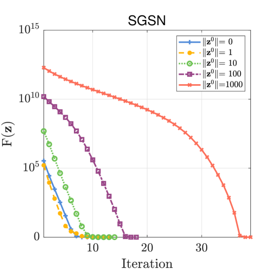
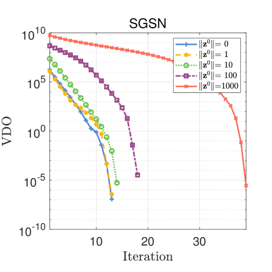
Figure 2: Convergence test for SGSN with different initial points.

$\bullet$ Test 0: On change of ${\bf z}^{0}$. This test aims to observe the basic convergence property of SGSN with different initial points ${\bf z}^{0}$. It is conducted on a simulated dataset with $q=1000$, $n=100$, $p=0.05$ and $r=0$. To produce different initial points for SGSN, we first generate a vector $\overline{{\bf z}}^{0}\in{\mathbb{R}}^{n}$ with entries being i.i.d. samples from the uniform distribution $U(0,1)$. Then we compute ${\bf z}^{0}=\rho\overline{{\bf z}}^{0}/\|\overline{{\bf z}}^{0}\|$ with $\rho\in\{0,1,10,100,1000\}$. SGSN starts with different ${\bf z}^{0}$ and the corresponding VDO and $F({\bf z})$ are recorded in Figure 2. The left panel in Figure 2 demonstrates the sufficient descent of $\{F({\bf z}^{k})\}_{k\in\mathbb{N}}$, which has been proved in Prop. 13. The right panel shows the descent of VDO , with a faster rate during the last few iterations. This phenomenon illustrates the global and local quadratic convergence of $\{{\bf z}^{k}\}_{k\in\mathbb{N}}$ given in Thms. 16 and 19.

Next, we test SGSN with ${\bf z}^{0}=0$ on simulated datasets with various $q$ (total number of samples), $n$ (number of features), $p$ (proportion of positive samples), and $r$ (noise ratio). For comparison, we select NM01 and CBN to solve the primal problem (1) and the dual problem (21) respectively. Their convergence performance can be measured by VDO and violation of primal optimality (VPO) respectively, where VPO is defined as follows:

$$\texttt{VPO}:=\max\left\{\|\nabla f({\bf x})+A^{\top}{\bf z}\|,~{\rm dist}\left(A{\bf x}+{\bf b},~{\rm Prox}_{\xi\bm{\mathcal{I}}(\cdot)}(A{\bf x}+{\bf b}+\xi{\bf z})\right)/\xi\right\},$$

where $\xi$ is a proximal parameter adjusted as the defaulted setting of NM01.

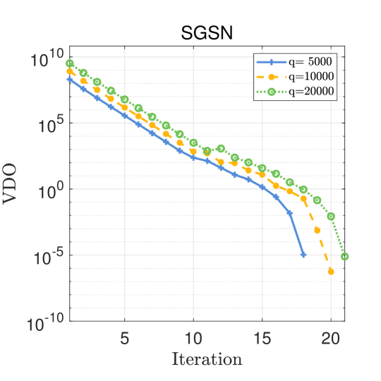
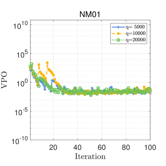
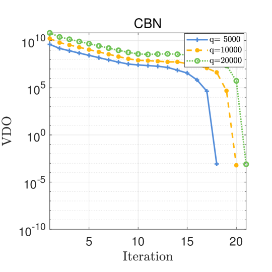
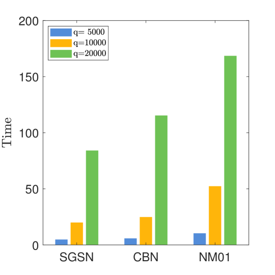
Figure 3: Convergence comparison on the simulated data with change of $q$.

$\bullet$ Test 1: On change of $q$. In this test, we generate datasets with $q\in\{5000,10000,20000\}$, $n=100$, $p=0.2$ and $r=0$. In this setting, $m$ (the number of rows in matrix $A$) is taken from $\{4\times 10^{6},1.6\times 10^{7},6.4\times 10^{7}\}$. SGSN and CBN demonstrate better convergence performance when dealing with these large-scale matrices. From Figure 3, we can also see that SGSN converges faster at the initial stage compared with CBN. At the final few steps, when the iterate is close to a P-stationary point of (21), VDO of SGSN rapidly drops below $10^{-4}$. In comparison, the VPO of NM01 decreases relatively faster during the first several iterations and then stagnates around $10^{-2}$. In this test, SGSN spends the shortest TIME to achieve the smallest VDO.

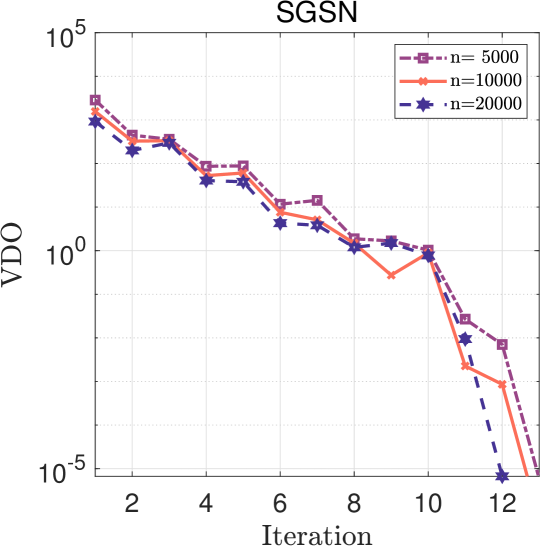
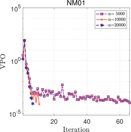
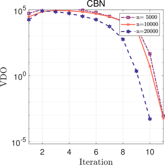
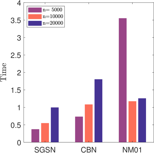
Figure 4: Convergence comparison on the simulated data with change of $n$.

$\bullet$ Test 2: On change of $n$. We take $n\in\{5000,10000,20000\}$, $q=1000$, $p=0.2$ and $r=0$. Figure 4 shows that all the algorithms converge very fast in the cases of $n\geq 10000$. When $n=5000$, NM01 requires more iterations for VPO to get below $10^{-4}$.

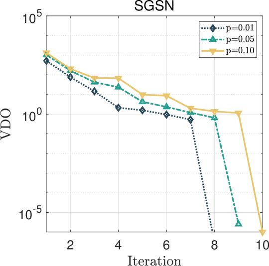
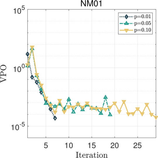
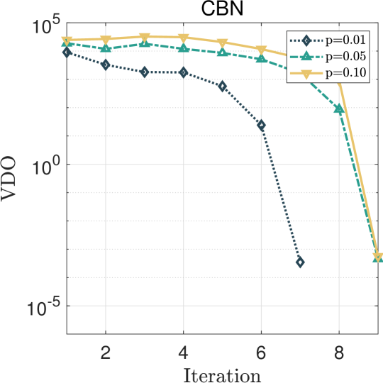
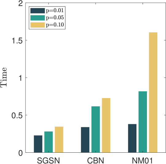
Figure 5: Convergence comparison on the simulated data with change of $p$.

$\bullet$ Test 3: On change of $p$. We alter $p\in\{0.01,0.05,0.1\}$, and fix $q=1000$, $n=10000$ and $r=0$. In all the cases, SGSN and CBN demonstrate significant decrease on VDO along with iteration. We also observe from Figure 5 that NM01 spends more TIME and requires more iterations when $p=0.05$ and $0.1$.

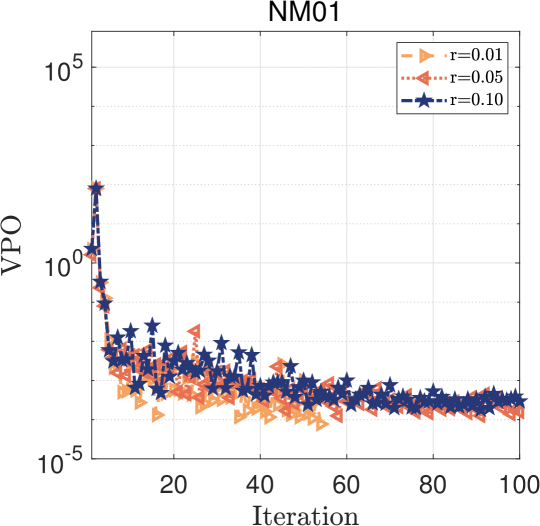
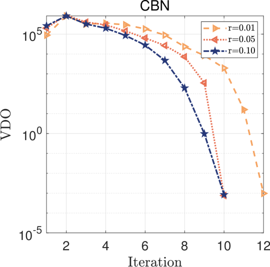
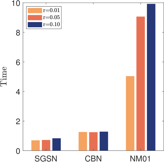
Figure 6: Convergence comparison on the simulated data with change of $r$.

$\bullet$ Test 4: On change of $r$. Finally, we test cases of $r\in\{0.01,0.05,0.1\}$, $q=1000$, $n=10000$ and $p=0.2$. As shown in Figure 6 again, compared with the other two algorithms, SGSN has the smallest VDO with the shortest TIME. The VPO of NM01 decreases faster over the first several iterations, and then fluctuates around $10^{-3}$.

5.1.2 Experiments on Real Dataset

In this part, we test SGSN and the three selected algorithms on the real datasets given in Table 1. For each dataset, five-fold cross-validation is conducted and the average value of AUC and TIME for each algorithm are recorded. As for the parameters of the comparison algorithms, NM01 adopts the default setting. The weighted parameter for the loss function in PRSVM and OPAUC is chosen from $\{10^{-3},10^{-2},\cdots,10^{3}\}$ with the highest AUC. Moreover, we stop SGSN and CBN when $\texttt{VDO}_{k}/\texttt{VDO}_{1}\leq 10^{-3}$ or $|\texttt{VDO}_{k}-\texttt{VDO}_{k-1}|<10^{-3}$, where $\texttt{VDO}_{k}$ denotes the violation of dual optimality at the $k$-th iterate. NM01 is terminated by a similar rule, replacing the above VDO with VPO.

Example 2

The details of real $\mbox{datasets}^{\mbox{\rm\scriptsize 1-4}}$ for AUC maximization are summarized in Table 1. All the datasets are preprocessed by feature-wise scaling to the interval $[-1,1]$.

Table 1: Real datasets for AUC maximization.

Abbreviation	Dataset	Domain	$q_{-}$	$q_{+}$	$m$	$n$
all	Allaml	Text	47	25	1175	7129
aou	AP_Ovary_Uterus	Biology	124	198	24552	10936
bas	Basehock	Text	999	994	993006	4862
col	Colon_Cancer	Biology	40	22	880	2000
duk	Duke	Biology	21	23	483	7129
gli	Gli85	Biology	26	59	1534	22283
gs2	Gse2280	Biology	5	22	110	11868
gs7	Gse7670	Biology	27	27	729	11868
leu	Leukemia	Biology	47	25	1175	7070
mad	Madelon	Artificial	1000	1000	1000000	500
ove	Ova_Endometrium	Biology	61	1484	90524	10936
ovk	Ova_Kidney	Biology	260	1285	334100	10936
ovo	Ova_Ovary	Biology	198	1347	266706	10936
pcm	Pcmac	Text	961	982	943702	3289
pro	Prostate_Ge	Biology	50	52	2600	5966
rel	Relathe	Text	648	779	504792	4322
smk	Smk_Can187	Biology	90	97	8730	19993
spl	Splice	Biology	483	517	249711	60

The comparison results are summarized in Table 2. We can observe that SGSN has a similar AUC but shorter TIME than NM01 or CBN because it is more effective in reducing the violation of optimality. Although the other two algorithms are also competitive on AUC, their TIME are longer than that of SGSN on most of the datasets. For example, on the dataset ovk, our SGSN only requires about $10\%$ of the TIME of PRSVM to achieve a higher AUC.

Table 2: Numerical results on real datasets for AUC maximization.

	AUC (%) $\uparrow$					TIME (sec) $\downarrow$
	SGSN	NM01	CBN	PRSVM	OPAUC	SGSN	NM01	CBN	PRSVM	OPAUC
all	99.00	99.00	99.00	98.00	98.50	2.677e-2	3.285e-2	3.980e-2	1.438e-1	1.961e+1
aou	94.48	94.75	94.46	94.18	94.16	2.773e-1	3.585e-1	4.819e-1	2.821e+0	1.950e+2
bas	98.82	97.82	98.46	98.73	98.76	1.868e+0	1.017e+1	3.077e+0	4.701e+0	2.335e+2
col	87.92	85.63	87.92	86.04	85.83	2.061e-2	1.085e-1	3.083e-2	7.766e-2	3.407e+0
duk	89.54	90.79	89.54	89.54	84.54	3.082e-2	4.377e-2	4.797e-2	1.517e-1	3.031e+1
gli	95.76	95.76	95.76	94.18	93.33	8.698e-2	1.100e-1	1.422e-1	4.148e-1	2.701e+2
gs2	61.67	61.67	61.67	61.67	56.67	1.556e-2	1.513e-2	2.031e-2	6.896e-2	1.999e+1
gs7	98.40	98.40	98.40	98.40	97.60	4.164e-2	3.406e-2	7.484e-2	1.333e-1	3.964e+1
leu	99.00	99.00	99.00	98.50	65.00	2.344e-2	2.690e-2	4.478e-2	1.665e-1	1.951e+1
mad	55.68	53.66	55.41	54.33	58.26	5.120e+0	1.300e+1	1.134e+1	3.154e+0	9.349e+0
ove	95.81	94.52	95.21	95.42	93.69	7.186e-1	2.379e+0	1.492e+0	2.012e+1	1.209e+3
ovk	99.16	98.95	99.11	99.09	98.26	1.251e+0	2.151e+0	2.314e+0	1.844e+1	1.288e+3
ovo	93.30	91.74	93.32	93.16	91.52	1.517e+0	2.367e+0	2.375e+0	4.341e+1	1.263e+3
pcm	91.11	88.73	90.56	90.40	90.26	1.669e+0	2.782e+1	5.701e+0	8.364e+0	1.468e+2
pro	96.00	95.60	96.00	95.80	90.33	3.279e-2	3.787e-1	5.935e-2	1.196e-1	2.401e+1
rel	93.28	90.88	92.14	92.57	92.44	1.336e+0	4.266e+0	6.050e+0	3.166e+0	1.456e+2
smk	78.76	77.93	77.81	78.04	76.49	1.217e+0	1.791e+0	4.312e-1	9.226e-1	4.819e+2
spl	88.28	88.39	88.23	88.23	87.19	1.909e-1	5.908e-1	5.429e-1	1.597e-1	1.845e-1

“$\uparrow$” means that a larger metric value corresponds to better algorithm performance, while “$\downarrow$” has the opposite meaning.

5.2 Sparse Multi-Label Classification

For a multi-label classification (MLC) problem with $\ell$ labels, let ${\bf c}_{i}\in{\mathbb{R}}^{d}$, $i\in[q]$ be the feature vector with its last entry $[{\bf c}_{i}]_{d}=1$ and class label ${\bf y}_{i}\in\{-1,1\}^{\ell}$ for $i\in[q]$. Then we denote matrices $\textbf{C}:=[{\bf c}_{1},\cdots,{\bf c}_{q}]^{\top}\in{\mathbb{R}}^{q\times d}$ and $\textbf{Y}:=[{\bf y}_{1},\cdots,{\bf y}_{q}]^{\top}\in{\mathbb{R}}^{q\times\ell}$. Given arbitrary feature vector ${\bf c}$, a linear binary relevance classifier ${\mathcal{H}}:{\mathbb{R}}^{d}\to{\mathbb{R}}^{\ell}$ returns a label vector by the following rule [12, 62]:

$${\mathcal{H}}({\bf c}):=\left({\rm sgn}({\bf c}^{\top}{\bf x}_{1}),\cdots,{\rm sgn}({\bf c}^{\top}{\bf x}_{\ell})\right),$$

where ${\bf x}:=({\bf x}_{1};\cdots;{\bf x}_{\ell})\in{\mathbb{R}}^{d\ell}$ is a weighted vector to be determined through optimizing certain loss function, and ${\rm sgn}:{\mathbb{R}}\to{\mathbb{R}}$ is the sign function, returning $1$ when the argument variable is positive and $-1$ otherwise. The Hamming loss (HL, see [66]) is an important evaluation metric in MLC. Let ${\bf y}^{(k)}=(y^{(k)}_{1},\cdots,y^{(k)}_{q})\in{\mathbb{R}}^{q}$ be the $k$-th column of the matrix Y, then Hamming loss for classifier ${\mathcal{H}}$ is defined as follows:

HL $$:=\frac{1}{q\ell}\sum_{i=1}^{q}\sum_{k=1}^{\ell}{\bf 1}_{(0,\infty)}(-y_{i}^{(k)}{\bf c}_{i}^{\top}{\bf x}_{k}).$$

When optimizing HL on the training data, a practical technique is to replace the above $-y_{i}^{(k)}{\bf c}_{i}^{\top}{\bf x}_{k}$ with $-y_{i}^{(k)}{\bf c}_{i}^{\top}{\bf x}_{k}+1$, see e.g. [62]. This helps to avoid trivial solution and improve generalization ability of the classifier. Meanwhile, when the dimension of the parameter ${\bf x}\in{\mathbb{R}}^{d\ell}$ is large, we can use sparse regularization to alleviate the risk of overfitting and reduce the dimension. Overall, we consider minimizing the Hamming loss with an elastic net regularizer. Denoting $m:=q\ell$ and $n:=d\ell$, this model is a special case of (1) with the following setting:

$$f({\bf x})=\frac{1}{2}\|{\bf x}\|^{2}+\lambda_{1}\|{\bf x}\|_{1},~A:=\left[\begin{array}[]{ccc}-({\bf y}^{(1)}{\bf e}^{\top}_{d})\odot\textbf{C}&&\\ &\ddots&\\ &&-({\bf y}^{(\ell)}{\bf e}^{\top}_{d})\odot\textbf{C}\end{array}\right],~{\bf b}={\bf e}_{m},$$

where $\|\cdot\|_{1}$ is the $\ell_{1}$ norm and $\odot$ is the Hadamard product.

We can compute the conjugate function

$$f^{*}({\bf v})=\sum_{i=1}^{n}\varphi(v_{i})\quad\hbox{~with~}\ \varphi(t):=\left\{\begin{aligned} &0,&&\mbox{~if~}|t|\leq\lambda_{1},\\ &(|t|-\lambda_{1})^{2}/2,&&\mbox{~if~}|t|>\lambda_{1},\end{aligned}\right.$$

and thus the corresponding gradient and generalized Jacobian are as follows:

$$\nabla f^{*}({\bf v})=\left\{{\bf r}\in{\mathbb{R}}^{n}:r_{i}=\left\{\begin{aligned} &v_{i}-\lambda_{1},&&\mbox{~if~}v_{i}>\lambda_{1}\\ &0,&&\mbox{~if~}|v_{i}|\leq\lambda_{1}\\ &v_{i}+\lambda_{1},&&\mbox{~if~}v_{i}<-\lambda_{1}\end{aligned}\right.\right\}$$

$$\partial^{2}f^{*}({\bf v})=\left\{\mbox{Diag}({\bf r}):{\bf r}\in{\mathbb{R}}^{n},r_{i}\in\left\{\begin{aligned} &1,&&\mbox{~if~}|v_{i}|>\lambda_{1}\\ &[0,1],&&\mbox{~if~}|v_{i}|=\lambda_{1}\\ &0,&&\mbox{~if~}|v_{i}|<\lambda_{1}\end{aligned}\right.\right\}.$$

Let ${\bf a}^{(i)}$ be the $i$-th column of $A$, our SGSN will solve the following dual problem:

$$\min_{{\bf z}\in{\mathbb{R}}^{m}}\ F({\bf z})=\sum_{i=1}^{n}\varphi(-\langle{\bf a}^{(i)},{\bf z}\rangle)-\langle{\bf b},{\bf z}\rangle+g({\bf z}).$$ (65)

Next, we discuss the convergence property when solving (65). One can verify that the elastic net regularizer is semi-algebraic by [8, Def. 5]. Assuming the sequence $\{{\bf z}^{k}\}_{k\in\mathbb{N}}$ is bounded, the whole sequence converges to a P-stationary point ${\bf z}^{*}$ of (65) according to Prop. 13. $\nabla f^{*}$ is semismooth. Denoting ${\mathcal{S}}^{*}:={\mathcal{S}}({\bf z}^{*})$ and $\Gamma^{*}:=\{i\in[n]:|\langle{\bf a}^{(i)},{\bf z}^{*}\rangle|>\lambda_{1}\}$, if we further assume that $A_{{\mathcal{S}}^{*}\Gamma^{*}}$ has full row rank, then for any $H\in\widehat{\partial}^{2}h({\bf z}^{*})$, we have ${\bf d}^{\top}H_{{\mathcal{S}}^{*}}{\bf d}=\|A^{\top}_{{\mathcal{S}}^{*}\Gamma^{*}}{\bf d}\|^{2}>0$ for any ${\bf d}\in{\mathbb{R}}^{|{\mathcal{S}}^{*}|}\backslash\{0\}$. This means Assumption 3 holds and $\{{\bf z}^{k}\}_{k\in\mathbb{N}}$ converges to ${\bf z}^{*}$ with local superlinear rate by Thm. 19.

In the following numerical experiments, we set ${\bf z}^{0}=0$, $\mu=10^{-5}$, $\gamma=10^{-2}$, $c_{1}=10^{-4}$ and $c_{2}=10^{8}$ for SGSN. The proximal parameter is adaptively chosen as $\tau_{k}=0.1^{j}$, where $j$ is the smallest natural number such that $F({\bf v}^{k})-F({\bf z}^{k})\geq 10^{-4}\|{\bf v}^{k}-{\bf z}^{k}\|^{2}$. The regularization parameter $\lambda_{1}$ is selected from $\{2^{-6},2^{-5},\cdots,2^{6}\}$. Other setting for SGSN is the same as that in the last subsection. We select three comparison algorithms for the MLC problem with $\ell_{1}$ norm or group sparse regularizer: LLFS from [29], MDFS from [65] and RFS from [49]. We adjust the sparse regularization parameters of the three algorithms to achieve better performance. They are selected from $\{10^{-6},10^{-5},\cdots,10^{6}\}$ for RFS and MDFS, and $\{2^{-6},2^{-5},\cdots,2^{6}\}$ for LLFS. Other parameters of the three algorithms are set the same as their default values. We use the Hamming loss (HL), computational time (TIME) and number of nonzero elements (NNE) of the solution to evaluate the performance of the algorithms.

5.2.1 Experiments on Simulated Dataset

To observe how the change of dimension influence the performance, we test all four algorithms on simulated datasets with various $q$, $d$ and $\ell$ generated as follows.

Example 3

We first generate a matrix $\overline{\textbf{C}}\in{\mathbb{R}}^{q\times(d-1)}$ with i.i.d elements being chosen from standard normal distribution $N(0,1)$, and then the feature matrix is computed by $\textbf{C}=[\overline{\textbf{C}},{\bf e}_{q}]$. Next, we generate a matrix $W\in{\mathbb{R}}^{d\times\ell}$ with each element chosen from the uniform distribution $U(-1,1)$, and then the label matrix is computed by $\textbf{Y}={\rm Sgn}(\textbf{C}W)$, where ${\rm Sgn}(\cdot)$ is the sign function for a matrix. Finally, $90\%$ of samples are randomly selected as training data and the rest is regarded as testing data.

Table 3: Numerical results on Example 3 with different $q$, $d$ and $\ell$.

	HL $\downarrow$				TIME (sec) $\downarrow$				NNE $\downarrow$
	SGSN	RFS	LLFS	MDFS	SGSN	RFS	LLFS	MDFS	SGSN	RFS	LLFS	MDFS
$q$	$d=6000,\ell=3$
1000	0.424	0.424	0.445	0.453	1.186	4.908	22.10	23.47	2874	7293	2750	2970
2000	0.397	0.419	0.394	0.434	2.295	19.82	32.94	42.41	4625	12870	5312	4716
3000	0.368	0.423	0.373	0.410	4.371	49.11	42.54	75.31	6097	15174	7620	6192
4000	0.339	0.428	0.340	0.402	7.818	93.03	52.79	126.8	7470	16235	9679	7560
5000	0.310	0.431	0.321	0.390	11.21	154.0	64.08	200.0	8524	16797	12726	8586
6000	0.300	0.428	0.319	0.395	14.15	239.6	86.30	295.3	9303	17161	17046	9378
$d$	$q=2500,\ell=3$
2500	0.304	0.438	0.331	0.376	2.809	19.37	8.118	20.14	4205	6362	5593	4237
4000	0.346	0.420	0.354	0.406	2.880	25.36	16.23	33.98	4942	9772	4988	5004
5500	0.375	0.422	0.370	0.419	3.235	30.94	29.96	49.35	5290	13152	5476	5362
7000	0.401	0.426	0.404	0.437	2.857	36.96	50.58	69.50	5416	16499	5755	5544
8500	0.406	0.431	0.401	0.437	3.311	41.69	77.83	95.52	5830	19755	6035	5967
10000	0.407	0.433	0.418	0.451	3.761	47.29	106.8	128.6	6147	23134	6322	6330
$\ell$	$q=1000,d=2000$
5	0.370	0.462	0.372	0.403	1.176	2.186	4.604	2.756	4207	5364	4732	4270
7	0.372	0.468	0.378	0.415	1.698	2.252	5.854	2.453	5872	8014	6455	5950
9	0.373	0.450	0.374	0.398	2.117	2.26	7.887	2.428	7528	10855	8030	7614
11	0.371	0.441	0.375	0.403	2.479	2.294	9.458	2.069	9166	13749	9832	9284
13	0.369	0.463	0.379	0.407	3.143	2.389	10.82	2.191	10872	16795	11601	10972
15	0.364	0.467	0.374	0.403	3.503	2.378	12.78	2.092	12560	19877	13194	12720

“$\downarrow$” means that a smaller metric value corresponds to better algorithm performance.

$\bullet$ On change of $q$. We fix $d=6000$, $\ell=3$, and select $q\in\{1000,2000,\cdots,6000\}$. We can observe from Table 3 that SGSN takes the shortest TIME in all the cases. In particular, SGSN is at least $6$ times faster than the second fastest algorithm LLFS. SGSN also finds the solution with the smallest NNE when $q>1000$. TIME and NNE increases when $q$ rises, whereas HL shows the opposite trend.

$\bullet$ On change of $d$. We fix $q=2500$, $\ell=3$, and select $d\in\{2500,4000,\cdots,10000\}$. In this test, SGSN achieves the best performance in all the cases. When feature dimension $d$ grows, SGSN has a relatively small increase on TIME. This indicates that SGSN may be more advantageous when applied to large-scale datasets.

$\bullet$ On change of $\ell$. We fix $q=1000$, $d=2000$, and select $\ell\in\{5,7,\cdots,15\}$. From Table 3, we can observe that SGSN has the best HL and NNE. Its TIME is also the shortest when $\ell\leq 9$, and slightly larger than that of RFS and MDFS when $\ell\geq 11$.

5.2.2 Experiments on Real Data

In this part, we test all the algorithms on real MLC problems listed in Table 4.

Example 4

The real datasets in Table 4 are available on the multi-label classification dataset repository. For each dataset, the partition in $67\%$ train and $33\%$ test is performed by following the Iterative Stratification method proposed by [58].

Table 4: Real multi-label classification datasets with higher dimension.

Abbreviation	Dataset	Domain	$q$	$d$	$\ell$	$q\times d\times\ell$
bbc	3s-bbc1000	Text	352	1000	6	2.11e+06
int	3s-inter3000	Text	169	3000	6	3.04e+06
eug	EukaryoteGO	Biology	7766	12689	22	2.17e+09
gng	GnegativeGO	Biology	1392	1717	8	1.91e+07
gnp	GnegativePseAAC	Biology	1392	440	8	4.90e+06
gpg	GpositiveGO	Biology	519	912	4	1.89e+06
gpp	GpositivePseAAC	Biology	519	440	4	9.13e+05
hup	HumanPseAAC	Biology	3106	440	14	1.91e+07
ima	Image	Image	2000	294	5	2.94e+06
med	Medical	Text	978	1449	45	6.38e+07
plg	PlantGO	Biology	978	3091	12	3.63e+07
plp	PlantPseAAC	Biology	978	440	12	5.16e+06
sch	Stackex$\_$chess	Text	1675	585	227	2.22e+08
sco	Stackex$\_$coffee	Text	225	1763	123	4.88e+07
vig	VirusGO	Biology	207	749	6	9.30e+05
vip	VirusPseAAC	Biology	207	440	6	5.46e+05
yar	Yahoo$\_$Arts	Text	7484	23146	26	4.50e+09
yed	Yahoo$\_$Education	Text	12030	27534	33	1.09e+10
yrr	Yahoo$\_$Recreation	Text	12830	30324	22	8.56e+09
yrf	Yahoo$\_$Reference	Text	8027	39679	33	1.05e+10

Table 5: Numerical results of all algorithms on real multi-label classification datasets.

	HL $\downarrow$				TIME (sec) $\downarrow$				NNE $\downarrow$
	SGSN	RSF	LLSF	MFDS	SGSN	RSF	LLSF	MFDS	SGSN	RSF	LLSF	MFDS
bbc	1.949e-1	1.949e-1	1.994e-1	2.426e-1	3.856e-2	1.364e-1	1.541e-1	8.103e-2	13	4224	58	5394
int	1.871e-1	1.871e-1	1.871e-1	1.988e-1	6.921e-2	1.169e-1	1.674e+0	4.506e-1	10	804	109	8814
gng	1.410e-2	4.935e-2	1.437e-2	6.291e-2	1.704e-1	2.078e+0	1.042e+0	3.584e+0	181	11160	79	72
gnp	7.674e-2	8.026e-2	8.080e-2	1.020e-1	9.605e-1	1.431e+0	8.913e-2	1.207e+0	120	3520	976	3512
gpg	3.343e-2	8.866e-2	3.052e-2	5.087e-2	5.279e-2	2.027e-1	1.170e-1	4.915e-1	77	2664	49	24
gpp	1.599e-1	2.137e-1	1.817e-1	2.965e-1	4.249e-1	1.650e-1	1.841e-2	2.311e-1	20	1760	490	56
hup	8.221e-2	8.242e-2	8.235e-2	9.286e-2	1.585e+0	9.824e+0	1.634e-1	8.181e+0	123	378	224	6146
ima	2.192e-1	2.473e-1	2.473e-1	2.834e-1	8.593e-1	1.026e+1	3.932e-2	3.695e+0	129	105	156	1175
med	1.024e-2	1.268e-2	1.031e-2	5.726e-2	7.167e-1	1.030e+0	1.001e+0	2.196e+0	2132	53505	1809	4545
plg	3.643e-2	8.658e-2	4.990e-2	8.832e-2	4.637e-1	1.503e+0	3.650e+0	5.607e+0	1515	4408	2584	3336
plp	8.458e-2	8.658e-2	8.658e-2	1.742e-1	2.042e+0	7.156e-1	4.372e-2	5.203e-1	25	192	52	5268
sch	9.958e-3	1.049e-2	9.640e-3	1.315e-2	2.187e+0	3.015e+0	1.774e+0	5.188e+0	115	21565	1910	227
sco	1.570e-2	1.581e-2	1.558e-2	1.581e-2	6.203e-1	2.562e-1	1.562e+0	1.426e+0	25	13644	123	1845
vig	2.412e-2	5.482e-2	3.289e-2	8.772e-2	7.366e-2	3.952e-2	6.714e-2	1.815e-1	288	2232	229	180
vip	1.842e-1	1.864e-1	1.908e-1	1.930e-1	1.866e-1	3.388e-2	2.749e-2	3.306e-1	25	114	50	1314
eug	2.015e-2	2.883e-2	2.022e-2	8.562e-2	1.496e+1	3.214e+2	1.131e+2	7.526e+2	2784	239316	1558	13948
yar	5.850e-2	6.469e-2	6.159e-2	6.205e-2	2.724e+1	4.590e+02	2.242e+3	1.133e+3	1046	4420	36491	2418
yed	3.980e-2	4.470e-2	4.070e-2	4.722e-2	4.426e+1	1.631e+03	2.761e+3	1.531e+3	680	13728	34962	891
yrr	5.173e-2	6.568e-2	6.357e-2	7.984e-2	4.367e+1	1.965e+03	2.703e+3	1.568e+3	1825	9108	20036	2684
yrf	2.628e-2	3.385e-2	2.671e-2	3.281e-2	3.479e+1	8.487e+02	2.924e+3	1.744e+3	1300	11451	85839	2640

“$\downarrow$” means that a smaller metric value corresponds to better the algorithm performance.

We report the performance of all the algorithms in terms of HL, TIME and NNE. Particularly, on the large-scale datasets yar, yed, yrr, yrf, we restrict the TIME of LLFS within 3000 seconds, because this algorithm takes longer time to terminate.

$\bullet$ On HL: We can see from Table 5 that SGSN has the best HL on almost all the datasets. LLFS also shows competitive HL, especially on datasets gpg and sco. RFS and MDFS have relatively larger HL.

$\bullet$ On TIME: SGSN shows significant advantage on TIME when solving large-scale dataset, such as eug, yar, yed, yrr, yrf. Particularly, on these datasets, TIME of SGSN is less than 1/10 of other algorithms. However, on the small dimensional datasets with $d<600$, LLFS has shorter TIME.

$\bullet$ On NNE: SGSN has the smallest NNE on most datasets in Table 5, especially on the high-dimensional datasets. The smaller NNE is, the faster SGSN runs because the subspace identified becomes smaller. This fact also accounts for the shortest TIME of SGSN used on the datasets yar, yed, yrr, yrf. For some low-dimensional datasets, such as gng and gpg, LLFS and MDFS find solutions with smaller NNE.

6 Conclusions

This paper proposes a new stationary duality approach for a class of composite optimization with indicator functions. The dual problem is constructed as $\ell_{0}$ regularized and nonnegativity constrained sparse optimization. The fundamental one-to-one correspondence between solutions of primal and dual problems is established. To find a dual solution, a subspace gradient semismooth Newton (SGSN) method is developed. It has low per-iteration complexity by exploiting the proximal operator of the sparse regularizer in the dual objective function. Moreover, SGSN enjoys global convergence with a local superlinear (or quadratic) rate under suitable conditions. Extensive experiments on the AUC maximization and multi-label classification problems demonstrate its competitive performance against top solvers for the respective problems.

Although the developed algorithm SGSN explicitly requires the gradient information of the conjugate function $f^{*}(\cdot)$, the stationary duality result does not rely on the availability of this piece of information. In theory, the stationary duality applies to general convex function $f$ as long as the dual problem admits an optimal solution. Numerically, this calls for further investigation when the gradient function cannot be cheaply computed. For instance, it would be interesting to see if derivative-free algorithms [17, 37] is a viable choice for the dual problem in this situation. If successful, it would significantly enlarge the applications of the stationary duality approach. We also note that the dual problem provides valuable information for the Lagrangian multiplier of the primal problem. It would be interesting to investigate whether a primal-dual method is possible. Those questions are not easy to answer and we leave them to our future research.

References

- [1] F. J. Aragón-Artacho, B. S. Mordukhovich, and P. Pérez-Aros, Coderivative-based semi-Newton method in nonsmooth difference programming, Math. Program., (2024), pp. 1–48.
- [2] H. Attouch, J. Bolte, P. Redont, and A. Soubeyran, Proximal alternating minimization and projection methods for nonconvex problems: An approach based on the Kurdyka-ojasiewicz inequality, Math. Oper. Res., 35 (2010), pp. 438–457.
- [3] A. Beck, First-Order Methods in Optimization, MOS-SIAM Series on Optimization, Society for Industrial and Applied Mathematics, Philadelphia, 2017.
- [4] A. Beck and M. Teboulle, A fast dual proximal gradient algorithm for convex minimization and applications, Oper. Res. Lett., 42 (2014), pp. 1–6.
- [5] G. Bento, B. Mordukhovich, T. Mota, and Y. Nesterov, Convergence of descent optimization algorithms under Polyak-ojasiewicz-Kurdyka conditions, 2025, https://optimization-online.org/wp-content/uploads/2025/02/Optimization-ModelFev2025.pdf.
- [6] R. Bhatia, Matrix analysis, Springer Science & Business Media, 2013.
- [7] J. Bolte, A. Daniilidis, A. Lewis, and M. Shiota, Clarke subgradients of stratifiable functions, SIAM J. Optim., 18 (2007), pp. 556–572.
- [8] J. Bolte, S. Sabach, and M. Teboulle, Proximal alternating linearized minimization for nonconvex and nonsmooth problems, Math. Program., 146 (2014), pp. 459–494.
- [9] J. Bolte, S. Sabach, and M. Teboulle, Nonconvex Lagrangian-based optimization: monitoring schemes and global convergence, Math. Oper. Res., 43 (2018), pp. 1210–1232.
- [10] R. I. Boţ, E. R. Csetnek, and D.-K. Nguyen, A proximal minimization algorithm for structured nonconvex and nonsmooth problems, SIAM J. Optim., 29 (2019), pp. 1300–1328.
- [11] R. I. Boţ and D.-K. Nguyen, The proximal alternating direction method of multipliers in the nonconvex setting: convergence analysis and rates, Math. Oper. Res., 45 (2020), pp. 682–712.
- [12] M. R. Boutell, J. Luo, X. Shen, and C. M. Brown, Learning multi-label scene classification, Pattern Recogn., 37 (2004), pp. 1757–1771.
- [13] O. Chapelle and S. S. Keerthi, Efficient algorithms for ranking with SVMs, Inf. Retr., 13 (2010), pp. 201–215.
- [14] G. Chen and M. Teboulle, A proximal-based decomposition method for convex minimization problems, Math. Program., 64 (1994), pp. 81–101.
- [15] X. Chen, L. Guo, Z. Lu, and J. J. Ye, An augmented Lagrangian method for non-Lipschitz nonconvex programming, SIAM J. Numer. Anal., 55 (2017), pp. 168–193.
- [16] F. H. Clarke, Optimization and nonsmooth analysis, SIAM, 1990.
- [17] A. R. Conn, K. Scheinberg, and L. N. Vicente, Introduction to derivative-free optimization, SIAM, 2009.
- [18] C. Cortes and V. Vapnik, Support-vector networks, Mach. Learn., 20 (1995), pp. 273–297.
- [19] Y. Cui, J. Liu, and J.-S. Pang, The minimization of piecewise functions: pseudo stationarity, arXiv preprint arXiv:2305.14798, (2023).
- [20] Y. Cui and J.-S. Pang, Modern nonconvex nondifferentiable optimization, SIAM, 2021.
- [21] F. Facchinei and J.-S. Pang, Finite-dimensional variational inequalities and complementarity problems, Springer, 2003.
- [22] M. Feng, J. E. Mitchell, J.-S. Pang, X. Shen, and A. Wächter, Complementarity formulations of -norm optimization problems, Pac. J. Optim., 14 (2018), pp. 273–305.
- [23] W. Gao, R. Jin, S. Zhu, and Z.-H. Zhou, One-pass AUC optimization, in International conference on machine learning, PMLR, 2013, pp. 906–914.
- [24] H. Gfrerer and J. V. Outrata, On a semismooth* Newton method for solving generalized equations, SIAM J. Optim., 31 (2021), pp. 489–517.
- [25] N. Hallak and M. Teboulle, An adaptive Lagrangian-based scheme for nonconvex composite optimization, Math. Oper. Res., 48 (2023), pp. 2337–2352.
- [26] A. K. Han, Non-parametric analysis of a generalized regression model: the maximum rank correlation estimator, J. Econom., 35 (1987), pp. 303–316.
- [27] S. Han, Y. Cui, and J.-S. Pang, Analysis of a class of minimization problems lacking lower semicontinuity, Math. Oper. Res., (2024), https://doi.org/10.1287/moor.2023.0295.
- [28] J. A. Hanley and B. J. McNeil, The meaning and use of the area under a receiver operating characteristic (ROC) curve., Radiology, 143 (1982), pp. 29–36.
- [29] J. Huang, G. Li, Q. Huang, and X. Wu, Learning label-specific features and class-dependent labels for multi-label classification, IEEE Trans. Knowl. Data Eng., 28 (2016), pp. 3309–3323.
- [30] C. Kanzow and T. Lechner, Globalized inexact proximal Newton-type methods for nonconvex composite functions, Comput. Optim. Appl., 78 (2021), pp. 377–410.
- [31] C. Kanzow and H.-D. Qi, A QP-free constrained Newton-type method for variational inequality problems, Math. Program., 85 (1999), pp. 81–106.
- [32] C. Kanzow, A. Schwartz, and F. Weiß, The sparse (st) optimization problem: reformulations, optimality, stationarity, and numerical results, Comput. Optim. Appl., 90 (2025), pp. 77–112.
- [33] M. G. Kendall, A new measure of rank correlation, Biometrika, 30 (1938), pp. 81–93.
- [34] P. D. Khanh, B. S. Mordukhovich, and V. T. Phat, A generalized Newton method for subgradient systems, Math. Oper. Res., 48 (2023), pp. 1811–1845.
- [35] P. D. Khanh, B. S. Mordukhovich, and V. T. Phat, Coderivative-based Newton methods in structured nonconvex and nonsmooth optimization, arXiv preprint arXiv:2403.04262, (2024).
- [36] P. D. Khanh, B. S. Mordukhovich, V. T. Phat, and D. B. Tran, Globally convergent coderivative-based generalized Newton methods in nonsmooth optimization, Math. Program., 205 (2024), pp. 373–429.
- [37] J. Larson, M. Menickelly, and S. M. Wild, Derivative-free optimization methods, Acta Numer., 28 (2019), pp. 287–404.
- [38] G. Li and T. K. Pong, Global convergence of splitting methods for nonconvex composite optimization, SIAM J. Optim., 25 (2015), pp. 2434–2460.
- [39] X. Li, D. Sun, and K.-C. Toh, A highly efficient semismooth Newton augmented Lagrangian method for solving lasso problems, SIAM J. Optim., 28 (2018), pp. 433–458.
- [40] H. Lütkepohl, Handbook of matrices, John Wiley & Sons, 1997.
- [41] B. S. Mordukhovich, Maximum principle in the problem of time optimal response with nonsmooth constraints, J. Appl. Math. Mech., 40 (1976), pp. 960–969.
- [42] B. S. Mordukhovich, Sensitivity analysis in nonsmooth optimization, Theor. Asp. Ind. Des., 58 (1992), pp. 32–46.
- [43] B. S. Mordukhovich, Variational Analysis and Generalized Differentiation. I. Basic Theory, II. Applications., Springer, Berlin, 2006.
- [44] B. S. Mordukhovich, Variational Analysis and Applications, Springer, 2018.
- [45] B. S. Mordukhovich, Second-Order Variational Analysis in Optimization, Variational Stability, and Control: Theory, Algorithms, Applications, Springer Nature, 2024.
- [46] B. S. Mordukhovich and M. E. Sarabi, Generalized Newton algorithms for tilt-stable minimizers in nonsmooth optimization, SIAM J. Optim., 31 (2021), pp. 1184–1214.
- [47] B. S. Mordukhovich, X. Yuan, S. Zeng, and J. Zhang, A globally convergent proximal Newton-type method in nonsmooth convex optimization, Math. Program., 198 (2023), pp. 899–936.
- [48] M. M. Münch, C. F. Peeters, A. W. Van Der Vaart, and M. A. Van De Wiel, Adaptive group-regularized logistic elastic net regression, Biostatistics, 22 (2021), pp. 723–737.
- [49] F. Nie, H. Huang, X. Cai, and C. Ding, Efficient and robust feature selection via joint -norms minimization, Advances in neural information processing systems, 23 (2010).
- [50] J. Nocedal and S. Wright, Numerical optimization, Springer series in operations research and financial engineering, Springer, New York, 2006.
- [51] R. Poliquin and R. T. Rockafellar, Tilt stability of a local minimum, SIAM J. Optim., 8 (1998), pp. 287–299.
- [52] B. T. Polyak, Gradient methods for the minimisation of functionals, USSR Comput. Math. Math. Phys., 3 (1963), pp. 864–878.
- [53] B. T. Polyak, Sharp minima, Institute of Control Sciences Lecture Notes, Moscow, (1979). Presented at the IIASA Workshop on Generalized Lagrangians and Their Applications, Laxenburg, Austria.
- [54] B. T. Polyak, Introduction to optimization, Optimization Software, New York, 1987.
- [55] L. Qi and J. Sun, A nonsmooth version of Newton’s method, Math. Program., 58 (1993), pp. 353–367.
- [56] R. T. Rockafellar, Convex Analysis, Princeton University Press, 1970.
- [57] R. T. Rockafellar and R. J.-B. Wets, Variational Analysis, Fundamental Principles of Mathematical Sciences, Springer, Berlin, 1998.
- [58] K. Sechidis, G. Tsoumakas, and I. Vlahavas, On the stratification of multi-label data, in Machine Learning and Knowledge Discovery in Databases: European Conference, Springer, 2011, pp. 145–158.
- [59] P. K. Shivaswamy and T. Jebara, Maximum relative margin and data-dependent regularization., J. Mach. Learn. Res., 11 (2010), pp. 747–788.
- [60] V. Vapnik, The nature of statistical learning theory, Springer science & business media, 1999.
- [61] F. Wang, W. Cao, and Z. Xu, Convergence of multi-block Bregman ADMM for nonconvex composite problems, Sci. China Inform. Sci., 61 (2018), pp. 1–12.
- [62] G. Wu, Y. Tian, and C. Zhang, A unified framework implementing linear binary relevance for multi-label learning, Neurocomputing, 289 (2018), pp. 86–100.
- [63] W. Xie and H. Yang, Group sparse recovery via group square-root elastic net and the iterative multivariate thresholding-based algorithm, AStA Adv. Stat. Anal., 107 (2023), pp. 469–507.
- [64] L. A. Zadeh, Fuzzy sets, Inf. Control, 8 (1965), pp. 338–353.
- [65] J. Zhang, Z. Luo, C. Li, C. Zhou, and S. Li, Manifold regularized discriminative feature selection for multi-label learning, Pattern Recogn., 95 (2019), pp. 136–150.
- [66] M.-L. Zhang and Z.-H. Zhou, A review on multi-label learning algorithms, IEEE Trans. Knowl. Data Eng., 26 (2013), pp. 1819–1837.
- [67] P. Zhang, N. Xiu, and Z. Luo, Zero-one composite optimization: Lyapunov exact penalty and a globally convergent inexact augmented Lagrangian method, Math. Oper. Res., 49 (2024), pp. 2602–2625.
- [68] Y. Zhang, N. Zhang, D. Sun, and K.-C. Toh, An efficient Hessian based algorithm for solving large-scale sparse group lasso problems, Math. Program., 179 (2020), pp. 223–263.
- [69] S. Zhou, L. Pan, and N. Xiu, Newton method for -regularized optimization, Numer. Algorithms, (2021), pp. 1–30.
- [70] S. Zhou, L. Pan, N. Xiu, and H.-D. Qi, Quadratic convergence of smoothing Newton’s method for 0/1 loss optimization, SIAM J. Optim., 31 (2021), pp. 3184–3211.
- [71] H. Zou and T. Hastie, Regularization and variable selection via the elastic net, J. R. Stat. Soc. Ser. B Methodol., 67 (2005), pp. 301–320.