Draft-based Approximate Inference for LLMs

Abstract

Optimizing inference for long-context Large Language Models (LLMs) is increasingly important due to the quadratic compute and linear memory complexity of Transformers. Existing approximation methods, such as key-value (KV) cache dropping, sparse attention, and prompt compression, typically rely on rough predictions of token or KV pair importance. We propose a novel framework for approximate LLM inference that leverages small draft models to more accurately predict the importance of tokens and KV pairs. Specifically, we introduce two instantiations of our proposed framework: (i) SpecKV, which leverages a draft output to accurately assess the importance of each KV pair for more effective KV cache dropping, and (ii) SpecPC, which uses the draft model’s attention activations to identify and discard unimportant prompt tokens. To the best of our knowledge, this is the first work to use draft models for approximate LLM inference acceleration, extending their utility beyond traditional lossless speculative decoding. We motivate our methods with theoretical and empirical analyses, and show a strong correlation between the attention patterns of draft and target models. Extensive experiments on long-context benchmarks show that our methods consistently achieve higher accuracy than existing baselines, while preserving the same improvements in memory usage, latency, and throughput. Our code is available at https://github.com/furiosa-ai/draft-based-approx-llm.

1 Introduction

The demand for longer context lengths in large language models (LLMs) gpt4 ; gemini25pro continues to grow liu2024lost , driven by applications such as dialogue systems (gpt4, ; gemini25pro, ), document summarization liu2020learning , and code completion code1 . Modern models like GPT-4 (gpt4, ) and Gemini-2.5-Pro gemini25pro have pushed context windows to over a million tokens. However, scaling Transformers transformer to these lengths remains difficult due to significant computational and memory constraints. Attention computation scales quadratically with context length, increasing inference latency, while key-value (KV) cache memory grows linearly, straining GPU resources. E.g., caching the KV states for 128K tokens in Llama-3.1-8B grattafiori2024llama can consume over 50GB of memory, limiting the practical scalability of LLMs.

To address scalability challenges, recent work introduces approximate LLM inference techniques that reduce latency and memory usage at inference time. Techniques include sparse attention for prefilling minference and decoding quest , which speed up inference by having each query attend to only a subset of keys. Sparse prefilling shortens time to the first token, while sparse decoding boosts generation throughput. KV cache dropping pyramidkv ; snapkv ; streamingllm ; h2o reduces memory and increases throughput by shrinking the cache after prefilling or during decoding. Prompt compression choi2024r2c ; llmlingua ; liskavets2024cpc further improves efficiency by removing unimportant tokens before inputting the prompt, reducing both attention and MLP computation, as well as decreasing KV cache size.

Orthogonally, speculative decoding (medusa, ; specdec2, ; hu2025speculativedecodingbeyondindepth, ; specdecode, ) accelerates LLM inference by using a small draft model to propose multiple tokens, which the target model verifies in parallel. This improves throughput without altering the output distribution and is particularly effective for autoregressive models, where sequential generation is a bottleneck. However, unlike approximate inference, speculative decoding does not lower the total memory or computation requirements and struggles with increasing context length.

In contrast, approximate LLM inference improves efficiency by reducing the amount of computation the model performs. This is often done by estimating the importance of each token or KV pair for future generation and discarding less important ones from attention or feedforward computations. Current methods (pyramidkv, ; adakv, ; minference, ; snapkv, ) use attention activations from input tokens to predict which tokens or KV pairs future tokens will attend to, as future tokens are not yet available. However, input attention activations alone do not reliably identify the tokens or KV pairs most relevant for future token generation.

In this work, we argue that token importance estimation can be improved by incorporating information from future tokens. To enable this without incurring the full cost of generating them, we introduce Draft-based Approximate Inference, a lookahead-based framework that uses a smaller, more efficient draft model to approximate future outputs with minimal overhead (Fig.˜1). By leveraging the context provided by this draft output, Draft-based Approximate Inference improves token importance estimates, enabling more accurate inference approximations. Our main contributions are as follows:

1. We present Draft-based Approximate Inference, the first framework to use draft model lookahead for enhanced approximate inference.

2. Within the Draft-based Approximate Inference framework, we develop two concrete algorithms targeting three LLM inference optimizations: Speculative KV Dropping (SpecKV) for KV cache dropping with sparse prefill, and Speculative Prompt Compression (SpecPC) for prompt compression.

3. We present theoretical analyses that establish both the rigorous justification and the anticipated effectiveness of our proposed methods.

4. We perform comprehensive experiments on long-context benchmarks, demonstrating that our methods attain state-of-the-art accuracy under fixed KV cache or prompt size constraints. Our results consistently outperform prior baselines (by up to 25 points on RULER ruler ), underscoring the potential of draft models for fast and accurate approximate inference in large language models.

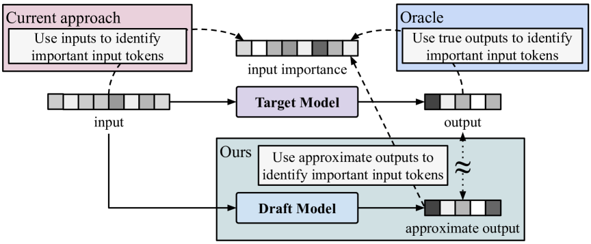
Figure 1: Overview of our Draft-based Approximate Inference framework for input token importance estimation. Unlike prior methods that rely only on input tokens, our approach incorporates draft model predictions of future output tokens, yielding more accurate importance estimates. This better aligns with the hypothetical oracle setting, where the true output is known and influential tokens can be precisely identified.

2 Related Work

Table 1: Summary of prior work. Complexity reported without auxiliary/draft model. ${n_{\text{in}}}$ and ${n_{\text{out}}}$ denote the number of input and output tokens, respectively. ${C_{\text{max}}}$ represents the maximum KV cache or prompt capacity. $s_{\text{prefill}}$ and $s_{\text{decode}}$ indicate the number of keys each query attends to during the prefill and decoding phases, respectively. Highlighted cells indicate improved complexity.

Type	Method	Sparse Attn	KV Dropping	Prefill Time	Decoding Time	Decoding Space
Dense	Dense	✗	✗	$O({n_{\text{in}}}^{2})$	$O({n_{\text{out}}}({n_{\text{in}}}+{n_{\text{out}}}))$	$O({n_{\text{in}}}+{n_{\text{out}}})$
Sparse attention	MInference minference , FlexPrefill flexprefill	Prefill	✗	$O({n_{\text{in}}}s_{\text{prefill}})$	$O({n_{\text{out}}}({n_{\text{in}}}+{n_{\text{out}}}))$	$O({n_{\text{in}}}+{n_{\text{out}}})$
	Quest quest , RetrievalAttention retrievalattention	Decode	✗	$O({n_{\text{in}}}^{2})$	$O({n_{\text{out}}}s_{\text{decode}})$	$O({n_{\text{in}}}+{n_{\text{out}}})$
KV dropping	StreamingLLM streamingllm	Prefill	Decode	$O({n_{\text{in}}}{C_{\text{max}}})$	$O({n_{\text{out}}}{C_{\text{max}}})$	$O({C_{\text{max}}})$
	H2O h2o	✗	Decode	$O({n_{\text{in}}}^{2})$	$O({n_{\text{out}}}{C_{\text{max}}})$	$O({C_{\text{max}}})$
	SnapKV snapkv , PyramidKV pyramidkv , AdaKV adakv	✗	After prefill	$O({n_{\text{in}}}^{2})$	$O({n_{\text{out}}}({C_{\text{max}}}+{n_{\text{out}}}))$	$O({C_{\text{max}}}+{n_{\text{out}}})$
	SpecKV (Ours)	Prefill	After prefill	$O({n_{\text{in}}}s_{\text{prefill}})$	$O({n_{\text{out}}}({C_{\text{max}}}+{n_{\text{out}}}))$	$O({C_{\text{max}}}+{n_{\text{out}}})$
Prompt compression	LLMLingua-2 pan2024llmlingua2 , CPC liskavets2024cpc , R2C choi2024r2c , SpecPC (Ours)	–	–	$O({C_{\text{max}}})$	$O({n_{\text{out}}}({C_{\text{max}}}+{n_{\text{out}}}))$	$O({C_{\text{max}}}+{n_{\text{out}}})$

Sparse Attention

One way to improve inference efficiency is through sparse attention with static patterns. For example, sliding window attention sliding_window , used in models like Mistral 7B (mistral7b, ) and Gemma 3 (gemma_2025, ), restricts each query to attend only a fixed-size window of recent keys, reducing computation and KV cache size during decoding. StreamingLLM (streamingllm, ) improves on sliding window by using initial tokens—called attention sinks—along with the sliding window. MInference (minference, ), adopted by Qwen2.5-1M (qwen2.5-1m, ), further boosts prefill efficiency by searching offline for adaptive sparse attention patterns—A-shape, Vertical-Slash, and Block-Sparse—assigned per head. FlexPrefill flexprefill extends this idea by determining sparsity rates for each input prompt. In contrast, Quest (quest, ) and RetrievalAttention retrievalattention target the decoding stage by only retrieving the most important KV pairs from the cache, reducing both memory bandwidth and computational demands during generation.

KV Cache Dropping

KV dropping reduces computation and memory during decoding. Sliding window attention sliding_window and StreamingLLM (streamingllm, ) are examples of KV dropping methods (as well as sparse attention) as they permanently evict KV pairs from cache. H2O (h2o, ) improves on this by dynamically selecting attention sinks, termed heavy-hitters, using attention scores at each decoding step, while also maintaining a sliding window. SnapKV (snapkv, ) compresses the KV cache at the end of the prefill stage by dropping unimportant KV pairs. Subsequent work extends this idea by allocating KV cache budgets non-uniformly across layers (PyramidKV (pyramidkv, )) and attention heads (AdaKV (adakv, ), HeadKV headkv ). However, these approaches drop tokens based only on current information, making them less robust to changes in token importance over time (sparse_frontier, ). In contrast, our method predicts future token importance using a draft model for more accurate importance estimation.

Prompt Compression

Prompt compression removes tokens before reaching the model, reducing compute and memory usage during both prefill and decoding—unlike KV dropping, which speeds up only decoding. It also surpasses sparse attention by saving both attention and MLP computation. Prompt compression works seamlessly with all types of inference setups, such as APIs or inference engines like vLLM vllm , since it does not require any modifications to the model. However, KV dropping can achieve higher compression because it selects tokens per head, while prompt compression drops the same tokens across all layers and heads.

In a question-answer setup, prompt compression may be question-agnostic (compressing context without considering the question) or question-aware (factoring in the question). Selective context li2023compressing and LLMLingua llmlingua are training-free, question-agnostic approaches using a small LLM to keep only key tokens. LongLLMLingua jiang2024longllmlingua adapts this for longer contexts in a question-aware manner. LLMLingua-2 pan2024llmlingua2 trains a small model conneau2020roberta to score token importance without using the question. CPC liskavets2024cpc uses a trained encoder to compute sentence importance via cosine similarity with the question, while R2C choi2024r2c splits the prompt into chunks, processes each with the question using a fine-tuned encoder-decoder Transformer (FiD izacard2021fid ), and ranks them via cross-attention.

Unlike CPC and R2C, our proposed SpecPC method imposes no constraints on prompt format and works seamlessly with any input or output accepted by the underlying draft model—including structured data, code, and visual modalities like image soft tokens. While prior methods are typically limited to sentence-level structures, single modalities, or text-only/image-only formats, SpecPC offers a unified and extensible approach that efficiently handles arbitrary and mixed-modal inputs.

Speculative Decoding

Speculative decoding (medusa, ; specdec2, ; hu2025speculativedecodingbeyondindepth, ; specdecode, ) emerged as an effective method for accelerating LLM inference. It leverages a small draft model to propose multiple tokens, which the full target model then verifies in parallel, increasing decoding throughput without changing the output distribution. This technique is especially advantageous for autoregressive models, where sequential token generation is a major bottleneck. Previous work further accelerates speculative decoding by enabling approximate inference in the draft model, using techniques such as sparse attention magicdec , KV dropping triforce , or KV cache quantization quantspec , all while preserving exact inference. In contrast, our approach is the first to leverage draft models for fast, approximate inference directly in the target model.

Table˜1 summarizes prior work, highlighting their prefill, decoding time, and memory complexities.

3 Proposed Framework: Draft-based Approximate Inference

Table 2: Comparison of speculative decoding and Draft-based Approximate Inference (ours).

Method	Memory	Latency	Compute	Aim
Speculative Decoding	✗	Decode	$\uparrow$	Increase hardware utilization
Draft-based Approximate Inference (Ours)	✓	All	$\downarrow$	Save compute and memory

Existing LLM approximation methods (pyramidkv, ; adakv, ; minference, ; snapkv, ) estimate the importance of current tokens on future generation by analyzing current attention patterns. While this can be effective, it provides only a rough estimate of each token’s importance. In contrast, if future tokens were available, we could make substantially better importance estimates by directly identifying which input tokens contribute to generating those output tokens. However, these future tokens are inaccessible before generation.

To overcome this, we propose a novel lookahead-based framework that leverages approximate future information to improve token importance estimation. Inspired by speculative decoding, we use a smaller draft model to generate an approximation of the future tokens.

Our goal fundamentally differs from speculative decoding (Table˜2). Speculative decoding improves hardware utilization by having a draft model propose tokens that the target model verifies, accelerating generation without changing the output distribution. However, it does not reduce total computation or memory usage.

In contrast, we reduce computation and memory costs by directly approximating the target model’s behavior. When the draft and target models are trained similarly, or if the draft is distilled hinton2015distilling from the target, their outputs and attention patterns typically align, making the draft output a reliable proxy for future tokens. This approximation enables more accurate importance estimation by revealing which input tokens have the greatest influence on the draft output.

This idea forms the basis of our Draft-based Approximate Inference framework (Fig.˜1), which we instantiate in two settings: SpecKV for KV cache dropping and sparse prefilling (Section˜4) and SpecPC for prompt compression (Section˜5).

4 SpecKV: Robust Importance Estimation for KV Cache Dropping

Existing sparse attention and KV cache dropping methods (minference, ; snapkv, ) estimate token importance by analyzing attention activations from the last ${n_{\text{window}}}$ queries to all keys. While this offers a rough approximation of future attention patterns, it can be inaccurate when the set of important KV pairs shifts over the course of generation. We argue that using attention activations from draft output queries to all keys yields a more robust and accurate estimate of KV pair importance.

4.1 Motivation for SpecKV

To guide both sparse prefilling and KV cache dropping, SpecKV estimates the importance of each KV pair in the input sequence. We define importance as the average attention activation from output queries to input keys. Specifically, the vector of importance scores and its approximation are given by

$$s^{T}=\tfrac{1}{{n_{\text{out}}}}\sum_{i=1}^{n_{\text{out}}}\operatorname{Softmax}\left(\tfrac{x_{i}^{(o)T}W_{q}W_{k}^{T}X^{T}}{\sqrt{d}}\right)\quad\text{and}\quad\hat{s}^{T}=\tfrac{1}{{n_{\text{out}}}}\sum_{i=1}^{n_{\text{out}}}\operatorname{Softmax}\left(\tfrac{\hat{x}_{i}^{(o)T}W_{q}W_{k}^{T}X^{T}}{\sqrt{d}}\right),$$ (1)

where $X=[x_{1},\dots,x_{n_{\text{in}}}]^{T}\in\mathbb{R}^{{n_{\text{in}}}\times d}$ is the matrix of input embeddings, $x_{i}^{(o)}\in\mathbb{R}^{d}$ is the $i$’th output embedding, and $\hat{x}_{i}^{(o)}\in\mathbb{R}^{d}$ is the $i$’th approximate output embedding (from the draft model). $s_{i}$ and $\hat{s}_{i}$ denote the importance of the $i$’th KV pair.

To understand when SpecKV provides reliable importance estimates, we analyze a simplified setting where the draft and target models produce similar embeddings. Specifically, we consider a single attention layer and assume that the output embeddings from the draft model are $\epsilon$-close (in $\ell_{2}$ norm) to those from the target model.

Theorem 1.

If $\|x_{i}^{(o)}-\hat{x}_{i}^{(o)}\|_{2}\leq\epsilon$ for all $i$ and $\|x_{j}\|_{2}\leq\sqrt{d}$ for all $j$, then $\|s-\hat{s}\|_{2}\leq\epsilon\|W_{q}W_{k}^{T}\|_{2}$.

This result shows that for a single attention layer, the worst-case error in the approximate importance scores is proportional to the worst-case error in the approximate output embeddings, implying that SpecKV provides reliable estimates as long as the draft model remains reasonably accurate (see Section˜B.1 for proof).

4.2 SpecKV Algorithm

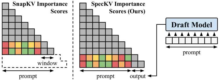
Figure 2: Overview of SpecKV: Instead of using only the last prompt tokens like SnapKV, SpecKV employs a lightweight draft model to generate lookahead tokens, providing richer context for more accurate KV importance estimation.

Figure 3: Importance scores estimated by SnapKV (top) and SpecKV (ours, bottom) on a sample from RULER S-NIAH-3 ruler , averaged across all heads. SpecKV exhibits stronger activations for important tokens relevant to the needle retrieval task. Lighter colors indicate higher attention activations and greater importance scores.

SpecKV (Algorithm˜1) begins by generating a draft output of length ${n_{\text{lookahead}}}$ using a small draft model, which acts as a proxy for the target model’s future outputs. During prefilling, both the input tokens and the draft tokens are passed through the target model. For each attention head, we compute token importance scores by measuring the cross-attention between the queries from the last ${n_{\text{window}}}$ input tokens and the draft output tokens to the remaining input keys (Fig.˜2). Using draft outputs allows SpecKV to better identify important tokens (Fig.˜3). We apply local pooling with kernel size $k$ to the attention scores to maintain continuity. These scores guide two optimizations: sparse prefilling and KV cache dropping. For sparse prefilling, we use a variation of the Vertical-Slash kernel pattern introduced in (minference, ). For KV cache dropping, we retain the top ${C_{\text{max}}}-{n_{\text{window}}}$ KV pairs with the highest importance scores, along with the final ${n_{\text{window}}}$ KV pairs from the most recent tokens.

5 SpecPC: Leveraging Draft Models for Efficient Prompt Compression

SpecKV leverages the output tokens of a lightweight draft model to enable more effective KV cache dropping, building upon the core assumption of speculative decoding that the draft and target models have similar output distributions. In this section, we take this approach further by directly utilizing the draft model’s attention activations to accelerate inference. Specifically, we introduce SpecPC, which compresses the prompt to achieve improved latency and reduced memory usage during both prefilling and decoding stages, surpassing the efficiency gains provided by traditional KV cache dropping.

5.1 Motivation for SpecPC

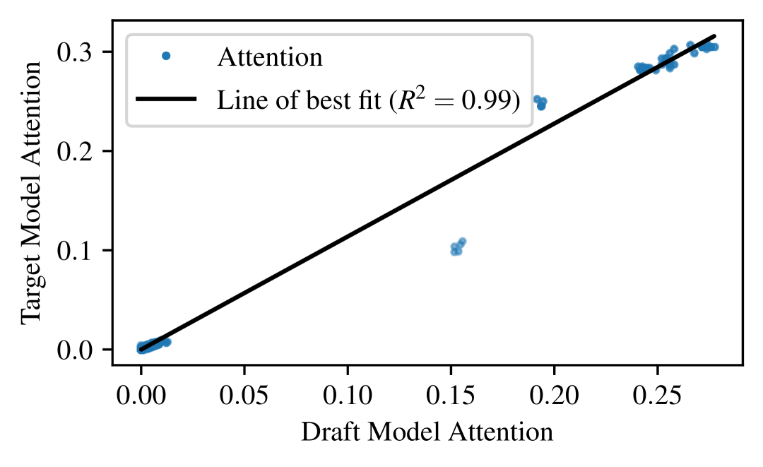
(a) Mean aggregation

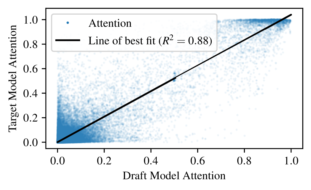
(b) Max aggregation

Figure 4: Correlation of attention activations between Llama-3.2-1B (draft) and Llama-3.1-8B (target) on 45 RULER (16K) ruler examples (five per each of nine tasks). Attention maps are aggregated across layers, heads, and queries using mean or max per key. Each point plots a key’s activation in the draft versus target model. Both aggregation methods ((a) mean, (b) max) reveal strong correlations.

Assuming the draft and target models produce similar outputs, we analyze the similarity of attention activations in a single attention layer.

The target model attention layer uses weights $W_{q}$, $W_{k}$, and $W_{v}$, and the draft model attention layer uses $\hat{W}_{q}$, $\hat{W}_{k}$, and $\hat{W}_{v}$. Let the input prompt be $X=[x_{1},\ldots,x_{n}]^{T}\in\mathbb{R}^{n\times d}$. The outputs of the target attention layer are

$$Y=\operatorname{Softmax}\left(\tfrac{XW_{q}W_{k}^{T}X^{T}}{\sqrt{d}}\right)XW_{v}=AXW_{v},$$ (2)

where $A=[a_{1},\ldots,a_{n}]^{T}$ is the attention matrix. Similarly, the outputs of the approximate (e.g., draft model) attention layer are

$$\hat{Y}=\operatorname{Softmax}\left(\tfrac{X\hat{W}_{q}\hat{W}_{k}^{T}X^{T}}{\sqrt{d}}\right)X\hat{W}_{v}=\hat{A}X\hat{W}_{v},$$ (3)

where $\hat{A}=[\hat{a}_{1},\ldots,\hat{a}_{n}]^{T}$ is the approximate attention matrix.

If the scaled inputs satisfy the Restricted Isometry Property (RIP) (rip, )—a condition widely studied in compressed sensing to ensure the stable recovery of sparse signals—we can establish the following bound:

Theorem 2.

If there exists a constant $c$ such that $cX^{T}$ satisfies the Restricted Isometry Property with parameters $2k$, $\delta$—where $k$ is the approximate sparsity of $a_{i}$ and $\hat{a}_{i}$—and the output error satisfies $\|y_{i}-\hat{y}_{i}\|_{2}\leq\epsilon\|X\|_{\infty,2}$, then the attention error satisfies $\|a_{i}-\hat{a}_{i}\|_{2}\leq\tfrac{2c\epsilon\|X\|_{\infty,2}}{\sigma_{\min}(W_{v})(1-\delta)}$.

This result offers a surprising and elegant connection: it reveals that mathematical tools developed for compressed sensing can also bound the error in attention approximations. Specifically, it shows that the worst-case error in the approximate attention activations is proportional to the worst-case error in the approximate outputs, with the constant depending on the conditioning of the weight matrices and the maximum input embedding norm. This implies that if the draft model provides a reasonable approximation of the output, it also gives a reasonable approximation of the attention activations (see Section˜B.2 for proof). Furthermore, even if the scaled inputs do not satisfy the RIP, we can still bound the attention approximation error by applying Theorem˜3 (see Section˜B.3 for proof).

In addition to theoretical analysis, we perform a small experiment to analyze the correlation of attention activations of Llama-3.2-1B (draft) and Llama-3.1-8B (target) in Fig.˜4 where we plot each draft model activation versus target model activation (see Fig.˜8 for additional models). The results show that their attention is highly correlated, further motivating our idea to use draft attention activations to approximate token importance.

5.2 SpecPC Algorithm

Based on our analysis, we present SpecPC (Algorithm˜2). SpecPC feeds an input prompt (length ${n_{\text{in}}}$) to the draft model and directly extracts its attention activations $A\in\mathbb{R}^{n_{\text{layer}}\times n_{\text{head}}\times\left({n_{\text{in}}}+{n_{\text{lookahead}}}-1\right)\times{n_{\text{in}}}}$, where $n_{\text{layer}}$ and $n_{\text{head}}$ denote the number of layers and heads. These activations indicate token importance and are used to drop less relevant tokens from the prompt.

Specifically, we use attention activations from the final (${n_{\text{window}}}+{n_{\text{lookahead}}}-1$) queries over each key, excluding the last ${n_{\text{window}}}$ keys, which are always retained. We skip the first ${l_{\text{skip}}}$ layers, as later layers provide more focused importance scores, while early layers attend broadly pyramidkv .

To aggregate per-token attention, we reweight queries based on proximity to the prompt’s end—later tokens get higher weights. Aggregation is performed across layers, heads, and queries to produce a single importance score per token (excluding the always-kept window). While mean aggregation shows superior attention correlation (Fig.˜4), max aggregation better prioritizes critical tokens and performs best in retrieval tasks.

We smooth aggregated scores with average pooling, then apply max pooling so that included tokens also bring their neighbors. This maintains the local context LLMs require. Unlike other methods that select entire sentences, we avoid sentence-level pre-processing to support non-text inputs, such as images. We then select the top-${C_{\text{max}}}$ tokens with the highest scores—always including window tokens—to form the compressed prompt, which is passed to the target model for generation.

6 Experiments

6.1 Setup

We evaluate SpecKV and SpecPC on two benchmarks: RULER ruler and LongBench longbench , comparing them against several baselines. For models, we use Qwen2.5-Instruct qwen2.5 (0.5B draft, 14B target) and Llama-3-Instruct grattafiori2024llama (3.2-1B draft, 3.1-8B target).

RULER is a synthetic benchmark with 13 tasks of varying complexity, including tasks such as key-value retrieval (NIAH), multi-hop tracing, and aggregation. It can be generated at any sequence length to assess a model’s effective context window. We evaluate at 4K, 8K, 16K, 32K, and 64K (Qwen is excluded at 64K due to its 32K sequence limit). LongBench contains 14 English, five Chinese, and two code tasks across five categories. We exclude the Chinese tasks (unsupported by Llama) and synthetic tasks (already covered by RULER).

For SpecKV, we compare against KV dropping methods—StreamingLLM streamingllm , H2O h2o , SnapKV snapkv , PyramidKV pyramidkv , and AdaKV adakv (Ada-SnapKV)—using a compression size (${C_{\text{max}}}$) of 256. Since layer-wise (PyramidKV) and head-wise (AdaKV) cache budgets can also be applied to SpecKV, we further evaluate AdaKV combined with SpecKV (Ada-SpecKV). For SpecPC, we benchmark against LLMLingua-v2 pan2024llmlingua2 , CPC liskavets2024cpc , and R2C choi2024r2c with ${C_{\text{max}}}=1024$. Based on our ablation studies (Fig.˜12), we set ${n_{\text{lookahead}}}$ to the maximum token limit for SpecKV and to one for SpecPC. See Appendix˜C for datasets and metrics, Appendix˜D for experimental details, and Appendix˜E for additional results, including evaluations with different ${C_{\text{max}}}$ values, more models, and multimodal experiments using Qwen2.5-VL qwen2.5-vl on the MileBench milebench image-text benchmark.

(a) KV dropping (${C_{\text{max}}}=256$)

(b) Prompt compression (${C_{\text{max}}}=1024$)

Figure 5: Performance of SpecKV and SpecPC on RULER compared to baselines. Both methods consistently outperform all baselines across sequence lengths. Notably, SpecPC closely matches the target model, maintaining strong results at longer contexts. Low-performing methods are omitted.

6.2 Results

Fig.˜5 (RULER), Table˜3 (LongBench Qwen), and Table˜4 (LongBench Llama), compare our methods with baselines. Both SpecKV and SpecPC consistently outperform other methods, demonstrating superior KV cache and prompt compression. Their performance far exceeds the draft model, highlighting robustness even with weaker drafts. Performance improves further with better drafts (Fig.˜11). On RULER, SpecKV exceeds baselines by up to 25 points and SpecPC nearly matches the target model, maintaining strong results even at longer context lengths. On LongBench, our methods excel in few-shot learning and code generation, where the draft output is especially valuable. Notably, for Qwen code completion, SpecPC even outperforms the target, suggesting prompt compression can improve performance by filtering out irrelevant context. For larger ${C_{\text{max}}}$, our methods remain superior (Fig.˜9; Tables˜9 and 10). Finally, multimodal (Section˜E.4) and additional model (Section˜E.6) evaluations further reaffirm the effectiveness and generality of our approach.

Table 3: LongBench performance with Qwen2.5-0.5B (draft) and Qwen2.5-14B (target).

	${C_{\text{max}}}$	Method	Single- doc QA	Multi- doc QA	Summary	Few-shot Learning	Code Completion	All
Dense	–	Draft	21.04	24.4	21.23	54.07	33.39	30.64
		Target	53.19	42.83	24.99	65.34	51.75	47.33
KV	256	StreamingLLM	38.66	24.13	19.10	49.75	35.23	33.24
		H2O	46.98	29.66	19.82	50.88	47.86	38.41
		SnapKV	49.07	33.19	19.49	54.49	47.34	40.25
		PyramidKV	47.07	31.84	18.32	54.81	43.26	38.76
		Ada-SnapKV	50.92	34.57	19.63	55.07	49.58	41.41
		SpecKV	51.07	38.76	23.20	59.68	49.58	44.09
		Ada-SpecKV	51.92	39.38	24.90	61.05	53.43	45.61
PC	1024	LLMLingua-2	27.10	23.74	22.57	35.85	37.62	28.79
		CPC	42.76	36.05	22.58	48.38	35.57	37.17
		R2C	46.43	37.42	22.64	47.21	29.48	37.15
		SpecPC	47.70	38.30	23.30	59.74	52.52	43.73

Table 4: LongBench performance with Llama-3.2-1B (draft) and Llama-3.1-8B (target).

	${C_{\text{max}}}$	Method	Single- doc QA	Multi- doc QA	Summary	Few-shot Learning	Code Completion	All
Dense	–	Draft	28.08	27.27	25.65	60.16	31.11	34.69
		Target	45.85	43.79	28.68	66.65	50.46	46.84
KV	256	StreamingLLM	38.69	27.12	21.64	50.75	34.74	34.58
		H2O	43.54	36.81	22.62	55.64	47.81	40.82
		SnapKV	43.79	37.31	21.96	56.29	47.34	40.91
		PyramidKV	43.62	37.79	21.75	55.15	46.32	40.54
		Ada-SnapKV	44.04	37.86	22.34	59.95	50.39	42.38
		SpecKV	43.23	39.73	24.43	60.90	51.09	43.36
		Ada-SpecKV	42.40	40.73	25.74	57.94	52.51	43.25
PC	1024	LLMLingua-2	29.61	24.83	23.43	24.18	40.66	27.68
		CPC	35.67	36.61	25.26	34.01	43.58	34.42
		R2C	38.41	39.07	25.28	43.26	43.99	37.58
		SpecPC	44.83	39.94	25.85	63.70	44.82	43.76

6.3 Performance

Fig.˜6 compares the latency of our proposed methods and several baselines using Qwen2.5-14B as the target model and Qwen2.5-0.5B as the draft model, running on a single NVIDIA H100 80GB GPU. We use ${n_{\text{lookahead}}}=64$ for SpecKV and ${n_{\text{lookahead}}}=1$ for SpecPC, matching our experimental setup in Section˜6.2. We measure latency up to the generation of the first target token (TTFT), including both the draft stage and any auxiliary models. SpecKV surpasses SnapKV due to sparse prefilling. Without this step, SpecKV is only slightly slower than SnapKV, indicating that the draft model adds minimal overhead. Other KV dropping methods are omitted, as their performance is similar to SnapKV. For prompt compression, our SpecPC method outperforms all baselines despite processing the full prompt at once. By contrast, methods like CPC and R2C split the prompt into smaller units to reduce attention complexity but require CPU-based text preprocessing, which increases overhead for longer sequences. Overall, prompt compression methods are faster than KV dropping, as only ${C_{\text{max}}}$ tokens are passed to the target model. Memory-wise, SpecKV is similar to SnapKV (with negligible overhead from draft weights), and SpecPC is more memory-efficient than R2C (see Section˜E.1).

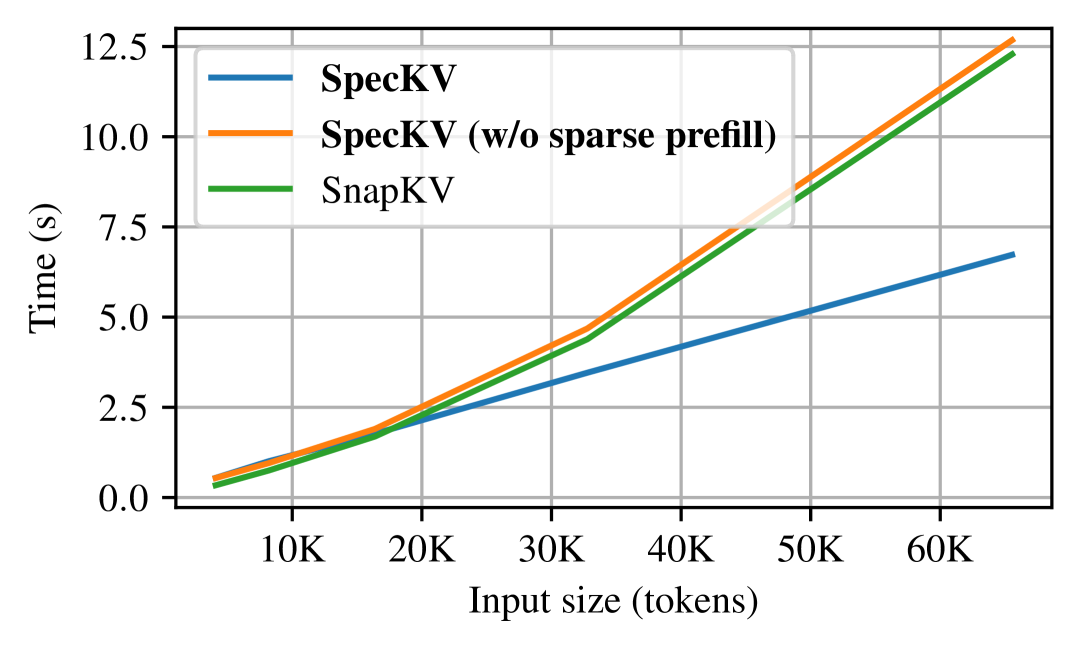
(a) KV dropping (${C_{\text{max}}}=256$)

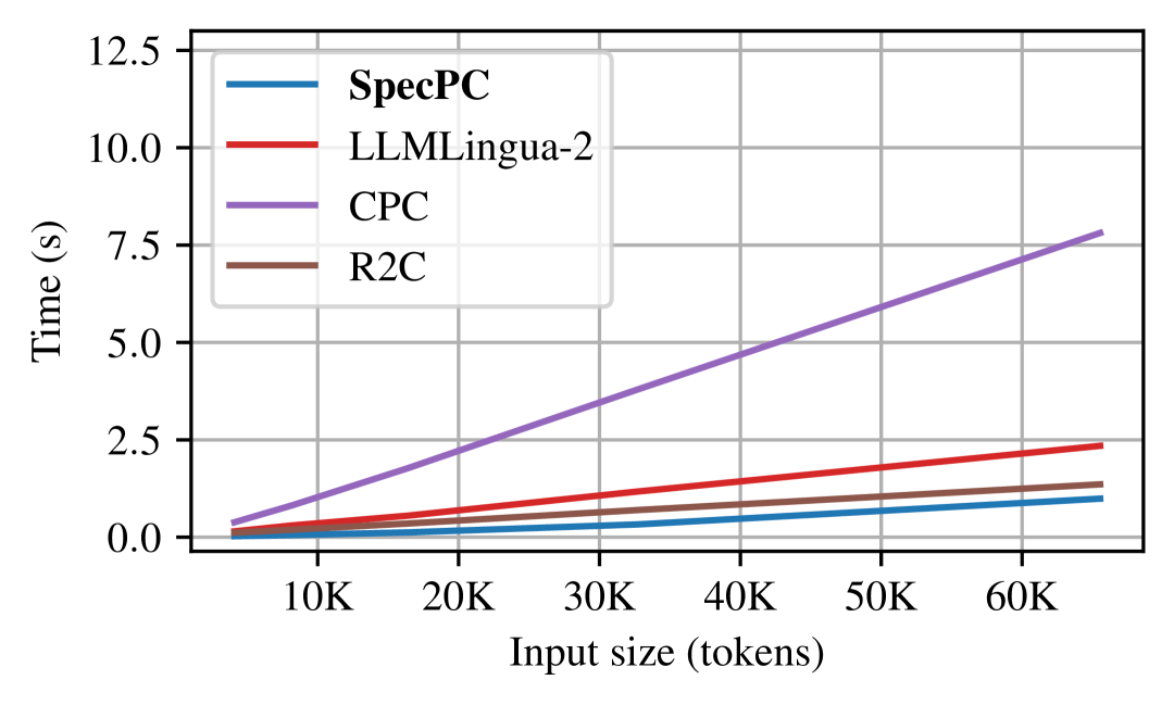
(b) Prompt compression (${C_{\text{max}}}=1024$)

Figure 6: Time-to-First-Token (TTFT) latency with SpecKV and SpecPC compared to various baseline methods (using Qwen2.5).

7 Discussion

In this paper, we introduced Draft-based Approximate Inference with Speculative KV Dropping (SpecKV) and Speculative Prompt Compression (SpecPC), the first methods to leverage draft models for accelerating long-context inference through KV cache dropping and prompt compression. Rooted in strong theoretical motivation, our techniques demonstrate clear advantages over existing baselines, achieving superior accuracy and reduced latency on standard long-context benchmarks. These results mark a significant advancement in expanding the utility of draft models beyond speculative decoding, opening new avenues for accurate and efficient approximate inference. We believe this line of research will prove increasingly vital as the demand for efficient long-context inference continues to grow.

Limitations and Future Work

For SpecKV, draft generation causes minimal latency. However, very long outputs or large ${n_{\text{lookahead}}}$ values may reduce performance. In these cases, lowering ${n_{\text{lookahead}}}$ could maintain speed with little loss in accuracy. For SpecPC, increasing ${n_{\text{lookahead}}}$ to generate more tokens led to only minor accuracy gains; better leveraging longer drafts remains future work.

Currently, Draft-based Approximate Inference supports sparse prefill, KV dropping, and prompt compression. Extensions such as lookahead-based sparse decoding or iterative KV cache dropping—where KV entries are periodically removed using draft lookahead—could further improve support for reasoning models with long outputs.

Appendix A Algorithms

Algorithm 1 SpecKV

1:Input:

2:    Input sequence $x$ with length ${n_{\text{in}}}$

3:    Parameters: Number of lookahead tokens ${n_{\text{lookahead}}}$, Maximum cache capacity ${C_{\text{max}}}$,

4:    Compression window size ${n_{\text{window}}}$, Kernel size $k$, Prefill window size ${n_{\text{slash}}}$,

5:    Number of global tokens in prefill ${n_{\text{vert}}}$    

6:Generate a draft output $y_{\text{draft}}$ of length ${n_{\text{lookahead}}}$ using the draft model.

7:Forward $x$ and $y_{\text{draft}}$ through the target model.

8:for each attention head in target model do

9:  $X\leftarrow\text{Target model hidden states from prompt at current layer}$ $\triangleright$ $X\in\mathbb{R}^{{n_{\text{in}}}\times d}$

10:  $Y\leftarrow\text{Target model hidden states from draft output at current layer}$ $\triangleright$ $Y\in\mathbb{R}^{{n_{\text{lookahead}}}\times d}$

11:  $m\leftarrow{n_{\text{in}}}-{n_{\text{window}}}$

12:  $A\leftarrow\operatorname{CrossAttention}\left(Q\text{ from }\left[\begin{smallmatrix}X_{m:}\\ Y\end{smallmatrix}\right],\;K/V\text{ from }X_{:m}\right)$ $\triangleright$ Compute attention

13:  $s\leftarrow\operatorname{MaxReduce}(A)$ $\triangleright$ $\mathbb{R}^{n_{1}\times n_{2}}\to\mathbb{R}^{n_{2}}$

14:  $s\leftarrow\operatorname{AvgPool1D}(s,k)$ $\triangleright$ Smooth attention

15:  $i_{\text{vert}}\leftarrow\operatorname{topk}(s,{n_{\text{vert}}})$ $\triangleright$ Select global tokens (Sparse prefill)

16:  $i_{\text{slash}}\leftarrow\{1,2,\ldots,{n_{\text{slash}}}\}$ $\triangleright$ Sliding window (Sparse prefill)

17:  $i_{\text{cache}}\leftarrow\operatorname{topk}(s,{C_{\text{max}}}-{n_{\text{window}}})\cup\{m+1,m+2,\ldots,{n_{\text{in}}}\}$ $\triangleright$ Select KVs

18:  $\text{output}\leftarrow\operatorname{VerticalSlash}(X,i_{\text{vert}},i_{\text{slash}})$ $\triangleright$ Sparse prefill attention

19:  $\text{cache}\leftarrow K_{i_{\text{cache}}},V_{i_{\text{cache}}}$ $\triangleright$ KV cache dropping

20:end for

Algorithm 2 SpecPC

1:Input:

2:    Draft attention tensor $A\in\mathbb{R}^{n_{\text{layer}}\times n_{\text{head}}\times\left({n_{\text{in}}}+{n_{\text{lookahead}}}-1\right)\times{n_{\text{in}}}}$

3:    Parameters: Window size ${n_{\text{window}}}$, Kernel size $k$, Number of neighbors ${n_{\text{neighbor}}}$,

4:    Number of selected tokens ${C_{\text{max}}}$, Number of skipped layers ${l_{\text{skip}}}$

5:$m\leftarrow{n_{\text{in}}}-{n_{\text{window}}}$

6:$A\leftarrow A_{l_{\text{skip}}:,:,m:,:m}$ $\triangleright$ Skip layers and only consider window queries and non-window keys

7:for $j\in\{1,2,\ldots,{n_{\text{window}}}\}$ do

8:  $A_{\ldots,j,:}\leftarrow\frac{i}{{n_{\text{window}}}}A_{\ldots,j,:}$ $\triangleright$ Assign more weight to later tokens

9:end for

10:$s\leftarrow\operatorname{MaxReduce}(A)$ $\triangleright$ $\mathbb{R}^{n_{1}\times n_{2}\times n_{3}\times n_{4}}\to\mathbb{R}^{n_{4}}$

11:$s\leftarrow\operatorname{AvgPool1D}(s,k)$ $\triangleright$ Smooth attention

12:$s\leftarrow\operatorname{MaxPool1D}(s,n_{\text{neighbor}})$ $\triangleright$ Keep neighbor tokens

13:$i_{\text{selected}}\leftarrow\operatorname{topk}(s,C_{\text{max}})\cup\{m+1,m+2,\ldots,{n_{\text{in}}}\}$ $\triangleright$ Keep most activated tokens and window tokens

14:return $i_{\text{selected}}$

Appendix B Deferred Proofs

Lemma 1.

$\|\operatorname{Softmax}(x)-\operatorname{Softmax}(y)\|_{2}\leq\|x-y\|_{\infty}$.

Proof.

Let $J$ be the Jacobian matrix of $\operatorname{Softmax}$. Then, $J(v)=\operatorname{diag}(p)-pp^{T}$, where $p=\operatorname{Softmax}(v)$. Note that $p$ is a probability distribution, so $p_{i}\geq 0$ for all $i$ and $\sum_{i}p_{i}=1$. For any vectors $v$ and $z$,

$$\|J(v)z\|_{2}^{2} = \|(\operatorname{diag}(p)-pp^{T})z\|_{2}^{2}$$

$$= \sum_{i}(p_{i}z_{i}-p_{i}p^{T}z)^{2}$$

$$= \sum_{i}p_{i}^{2}(z_{i}-p^{T}z)^{2}$$

$$\leq \sum_{i}p_{i}(z_{i}-p^{T}z)^{2}$$

$$= \sum_{i}\left(p_{i}z_{i}^{2}-2p_{i}z_{i}p^{T}z+p_{i}(p^{T}z)^{2}\right)$$

$$= \sum_{i}p_{i}z_{i}^{2}-(p^{T}z)^{2}$$

$$\leq \sum_{i}p_{i}z_{i}^{2}$$

$$\leq \sum_{i}p_{i}\|z\|_{\infty}^{2}$$

$$\leq \|z\|_{\infty}^{2}.$$

Thus, $\|J(v)z\|_{2}\leq\|z\|_{\infty}$ for all $v$ and $z$. From the fundamental theorem of line integrals,

$$\operatorname{Softmax}(x)-\operatorname{Softmax}(y)=\int_{0}^{1}J(y+t(x-y))(x-y)dt.$$ (4)

Finally,

$$\|\operatorname{Softmax}(x)-\operatorname{Softmax}(y)\|_{2} = \left\|\int_{0}^{1}J(y+t(x-y))(x-y)dt\right\|_{2}$$

$$\leq \int_{0}^{1}\|J(y+t(x-y))(x-y)\|_{2}dt$$

$$\leq \int_{0}^{1}\|x-y\|_{\infty}dt$$

$$= \|x-y\|_{\infty}.$$

∎

Lemma 2.

Let $y=\operatorname{Softmax}(x)$ and $y^{\prime}=\operatorname{Softmax}(x^{\prime})$. If $\|y-y^{\prime}\|_{p}\leq\epsilon$, then there exists a scalar $c$ such that $\|x-x^{\prime}-c\mathbf{1}\|_{p}\leq\tfrac{\epsilon}{m}$, where $m=\min_{i}(\min(y_{i},y_{i}^{\prime}))$ and $p\in\{1,2,\ldots,\infty\}$.

Proof.

From the mean value theorem, there exists $\xi\in(y_{i},y_{i}^{\prime})$ such that

$$\tfrac{\log y_{i}-\log y_{i}^{\prime}}{y_{i}-y_{i}^{\prime}}=\tfrac{d\log t}{dt}\Bigg{|}_{t=\xi}=\tfrac{1}{\xi}.$$ (5)

Note that $\xi>0$. Then,

$$|\log y_{i}-\log y_{i}^{\prime}|=\tfrac{1}{\xi}|y_{i}-y_{i}^{\prime}|\leq\tfrac{1}{m}|y_{i}-y_{i}^{\prime}|.$$ (6)

Let $c=\log\sum_{j}e^{x_{j}}-\log\sum_{j}e^{x_{j}^{\prime}}$, so

$$\left|\log\tfrac{e^{x_{i}}}{\sum_{j}e^{x_{j}}}-\log\tfrac{e^{x_{i}^{\prime}}}{\sum_{j}e^{x_{j}^{\prime}}}\right|=\left|x_{i}-x_{i}^{\prime}-\left(\log\sum_{j}e^{x_{j}}-\log\sum_{j}e^{x_{j}^{\prime}}\right)\right|=|x_{i}-x_{i}^{\prime}-c|$$ (7)

for all $i$. Thus,

$$|x_{i}-x_{i}^{\prime}-c|\leq\tfrac{1}{m}|y_{i}-y_{i}^{\prime}| \implies|x_{i}-x_{i}^{\prime}-c|^{p}\leq\tfrac{1}{m^{p}}|y_{i}-y_{i}^{\prime}|^{p}$$

$$\implies\sum_{i}|x_{i}-x_{i}^{\prime}-c|^{p}\leq\tfrac{1}{m^{p}}\sum_{i}|y_{i}-y_{i}^{\prime}|^{p}$$

$$\implies\|x-x^{\prime}-c\mathbf{1}\|_{p}^{p}\leq\tfrac{1}{m^{p}}\|y-y^{\prime}\|_{p}^{p}$$

$$\implies\|x-x^{\prime}-c\mathbf{1}\|_{p}\leq\tfrac{1}{m}\|y-y^{\prime}\|_{p}$$

$$\implies\|x-x^{\prime}-c\mathbf{1}\|_{p}\leq\tfrac{\epsilon}{m}.$$

∎

B.1 Proof of Theorem˜1

We define the vector of importance scores as and its approximation as

$$s^{T}=\tfrac{1}{{n_{\text{out}}}}\sum_{i=1}^{n_{\text{out}}}\operatorname{Softmax}\left(\tfrac{x_{i}^{(o)T}W_{q}W_{k}^{T}X^{T}}{\sqrt{d}}\right)\quad\text{and}\quad\hat{s}^{T}=\tfrac{1}{{n_{\text{out}}}}\sum_{i=1}^{n_{\text{out}}}\operatorname{Softmax}\left(\tfrac{\hat{x}_{i}^{(o)T}W_{q}W_{k}^{T}X^{T}}{\sqrt{d}}\right),$$ (8)

where $X=[x_{1},\dots,x_{n_{\text{in}}}]^{T}\in\mathbb{R}^{{n_{\text{in}}}\times d}$ is the matrix of input embeddings, $x_{i}^{(o)}\in\mathbb{R}^{d}$ is the $i$’th output embedding, and $\hat{x}_{i}^{(o)}\in\mathbb{R}^{d}$ is the $i$’th approximate output embedding (from the draft model). $s_{i}$ and $\hat{s}_{i}$ denote the importance of the $i$’th KV pair. In practice, SpecKV estimates importance using queries from recent input and draft output tokens. This is omitted from the theoretical analysis for clarity.

Proof.

We assume $\|x_{i}^{(o)}-\hat{x}_{i}^{(o)}\|_{2}\leq\epsilon$ for all $i$ and $\|x_{j}\|_{2}\leq\sqrt{d}$ for all $j$.

$\|x_{i}^{(o)}-\hat{x}_{i}^{(o)}\|_{2}\leq\epsilon$, so

$$\left|\tfrac{x_{i}^{(o)T}W_{q}W_{k}^{T}x_{j}}{\sqrt{d}}-\tfrac{\hat{x}_{i}^{(o)T}W_{q}W_{k}^{T}x_{j}}{\sqrt{d}}\right| = \tfrac{1}{\sqrt{d}}\left|(x_{i}^{(o)}-\hat{x}_{i}^{(o)})^{T}W_{q}W_{k}^{T}x_{j}\right|$$

$$\leq \tfrac{1}{\sqrt{d}}\|W_{q}W_{k}^{T}\|_{2}\epsilon\sqrt{d}$$

$$= \epsilon\|W_{q}W_{k}^{T}\|_{2}.$$

Thus,

$$\left\|\tfrac{x_{i}^{(o)T}W_{q}W_{k}^{T}X^{T}}{\sqrt{d}}-\tfrac{\hat{x}_{i}^{(o)T}W_{q}W_{k}^{T}X^{T}}{\sqrt{d}}\right\|_{\infty}\leq\epsilon\|W_{q}W_{k}^{T}\|_{2}.$$ (9)

Applying Lemma˜1 and the triangle inequality, we get

$$\|s-\hat{s}\|_{2} = \left\|\tfrac{1}{{n_{\text{out}}}}\sum_{i=1}^{n_{\text{out}}}\operatorname{Softmax}\left(\tfrac{x_{i}^{(o)T}W_{q}W_{k}^{T}X^{T}}{\sqrt{d}}\right)-\tfrac{1}{{n_{\text{out}}}}\sum_{i=1}^{n_{\text{out}}}\operatorname{Softmax}\left(\tfrac{\hat{x}_{i}^{(o)T}W_{q}W_{k}^{T}X^{T}}{\sqrt{d}}\right)\right\|_{2}$$

$$\leq \tfrac{1}{{n_{\text{out}}}}\sum_{i=1}^{n_{\text{out}}}\left\|\operatorname{Softmax}\left(\tfrac{x_{i}^{(o)T}W_{q}W_{k}^{T}X^{T}}{\sqrt{d}}\right)-\operatorname{Softmax}\left(\tfrac{\hat{x}_{i}^{(o)T}W_{q}W_{k}^{T}X^{T}}{\sqrt{d}}\right)\right\|_{2}$$

$$\leq \tfrac{1}{{n_{\text{out}}}}\sum_{i=1}^{n_{\text{out}}}\left\|\tfrac{x_{i}^{(o)T}W_{q}W_{k}^{T}X^{T}}{\sqrt{d}}-\tfrac{\hat{x}_{i}^{(o)T}W_{q}W_{k}^{T}X^{T}}{\sqrt{d}}\right\|_{\infty}$$

$$\leq \epsilon\|W_{q}W_{k}^{T}\|_{2},$$

∎

B.2 Proof of Theorem˜2

$$X=[x_{1},\ldots,x_{n_{\text{in}}}]^{T}$$ (10)

$$Y=[y_{1},\ldots,y_{n_{\text{in}}}]^{T}=\operatorname{Softmax}\left(\tfrac{XW_{q}W_{k}^{T}X^{T}}{\sqrt{d}}\right)XW_{v}$$ (11)

$$\hat{Y}=[\hat{y}_{1},\ldots,\hat{y}_{n_{\text{in}}}]^{T}=\operatorname{Softmax}\left(\tfrac{X\hat{W}_{q}\hat{W}_{k}^{T}X^{T}}{\sqrt{d}}\right)X\hat{W}_{v}$$ (12)

$$A=[a_{1},\ldots,a_{n_{\text{in}}}]^{T}=\operatorname{Softmax}\left(\tfrac{XW_{q}W_{k}^{T}X^{T}}{\sqrt{d}}\right)$$ (13)

$$\hat{A}=[\hat{a}_{1},\ldots,\hat{a}_{n_{\text{in}}}]^{T}=\operatorname{Softmax}\left(\tfrac{X\hat{W}_{q}\hat{W}_{k}^{T}X^{T}}{\sqrt{d}}\right)$$ (14)

Proof.

We assume $\|y_{i}-\hat{y}_{i}\|_{2}\leq\epsilon\|X\|_{\infty,2}$, where $\|X\|_{\infty,2}$ is the maximum $\ell_{2}$ norm of the rows of $X$. Additionally, we assume that there exists a constant $c$ such that $cX^{T}$ has the Restricted Isometry Property [8] with parameters $2k$, $\delta$, where $k$ is the approximate sparsity of $a_{i}$ and $\hat{a}_{i}$.

Recall that a matrix $B$ satisfies the Restricted Isometry Property with constant $\delta\in(0,1)$ if for every $k$-sparse vector $v$, the following inequality holds:

$$(1-\delta)\|v\|_{2}^{2}\leq\|Bv\|_{2}^{2}\leq(1+\delta)\|v\|_{2}^{2}.$$ (15)

Let $\Delta W_{v}=W_{v}-\hat{W}_{v}$ and $\Delta a_{i}=a_{i}-\hat{a}_{i}$.

If ${n_{\text{in}}}=1$, then $A=\hat{A}\in\mathbb{R}^{1\times 1}$ with $A_{1,1}=\hat{A}_{1,1}=1$, so $AX=\hat{A}X=X=x_{1}^{T}$, which implies

$$\|y_{1}-\hat{y}_{1}\|_{2}=\|x_{1}^{T}W_{V}-x_{1}^{T}\hat{W}_{v}\|_{2}=\|x_{1}^{T}\Delta W_{v}\|_{2}\leq\epsilon\|X\|_{\infty,2}=\epsilon\|x_{1}\|_{2}$$ (16)

for all $x_{1}$. $\|x_{1}^{T}W_{v}\|_{2}\leq\epsilon\|x_{1}\|$ for all $x_{1}$ is the definition of the matrix $\ell_{2}$ norm, so $\|\Delta W_{v}\|_{2}\leq\epsilon$.

$$\|y_{i}-\hat{y}_{i}\|_{2} = \|a_{i}^{T}XW_{v}-\hat{a}_{i}^{T}X\hat{W}_{v}\|_{2}$$

$$= \|a_{i}^{T}XW_{v}-(\hat{a}_{i}^{T}XW_{v}-\hat{a}_{i}^{T}X\Delta W_{v})\|_{2}$$

$$= \|a_{i}^{T}XW_{v}-(a_{i}^{T}XW_{v}-\Delta a_{i}^{T}XW_{v}-\hat{a}_{i}^{T}X\Delta W_{v})\|_{2}$$

$$= \|\Delta a_{i}^{T}XW_{v}+\hat{a}_{i}^{T}X\Delta W_{v}\|_{2}$$

$$\leq \epsilon\|X\|_{\infty,2}$$

Then, $\|\Delta a_{i}^{T}XW_{v}\|_{2}\leq\epsilon\|X\|_{\infty,2}+\|\hat{a}_{i}^{T}X\Delta W_{v}\|_{2}$.

Since $\hat{a}_{i}^{T}X$ is a convex combination of the rows of $X$, $\|\hat{a}_{i}^{T}X\|_{2}\leq\|X\|_{\infty,2}$.

Thus, $\|\Delta a_{i}^{T}XW_{v}\|_{2}\leq\epsilon\|X\|_{\infty,2}+\|\hat{a}_{i}^{T}X\Delta W_{v}\|_{2}\leq\epsilon\|X\|_{\infty,2}+\|\hat{a}_{i}^{T}X\|_{2}\|\Delta W_{v}\|_{2}\leq 2\epsilon\|X\|_{\infty,2}$.

Attention scores are approximately sparse [25], especially for long sequences. Therefore, we assume $a_{i}$ and $\hat{a}_{i}$ are $k$-sparse. Then, $\Delta a_{i}$ is at most $2k$-sparse. Since $cX^{T}$ has the Restricted Isometry Property with parameters $2k$, $\delta$,

$$(1-\delta)\|\Delta a_{i}\|_{2}\leq\|\Delta a_{i}^{T}(cX)\|_{2}\leq(1+\delta)\|\Delta a_{i}\|_{2}.$$ (17)

Then,

$$\tfrac{1}{c}(1-\delta)\|\Delta a_{i}\|_{2}\leq\|\Delta a_{i}^{T}X\|_{2}\leq\tfrac{2\epsilon\|X\|_{\infty,2}}{\sigma_{\min}(W_{v})},$$ (18)

so

$$\|\Delta a_{i}\|_{2}\leq\tfrac{2c\epsilon\|X\|_{\infty,2}}{\sigma_{\min}(W_{v})(1-\delta)}.$$ (19)

∎

B.3 Proof of Theorem˜3

Theorem 3.

If $\|Y-\hat{Y}\|_{2}\leq\epsilon\|X\|_{2}$ for all $X$ and the column space of $W_{q},W_{k},\hat{W}_{q},\hat{W}_{k}$ is a subset of the column space of $W_{v}$, then $\|a_{i}-\hat{a}_{i}\|_{2}\leq\epsilon\delta$, where

$$\delta=2d\tfrac{\sigma_{\max}(W_{v})^{2}}{\sigma_{\min}(W_{v})}\exp\left(2\max\left(\tfrac{\|W_{q}\|_{2}\|W_{k}\|_{2}}{\sigma_{\min}(W_{v})^{2}},\tfrac{\|\hat{W}_{q}\|_{2}\|\hat{W}_{k}\|_{2}}{\sigma_{\min}(\hat{W}_{v})^{2}}\right)\right)\|X\|_{\infty,2}^{2}.$$ (20)

Proof.

We assume $\|Y-\hat{Y}\|_{2}\leq\epsilon\|X\|_{2}$. Additionally, we assume that the column space of $W_{q},W_{k},\hat{W}_{q},\hat{W}_{k}$ is a subset of the column space of $W_{v}$. To get a norm bound on $\Delta a_{i}=a_{i}-\hat{a}_{i}$, we will bound the norms of the error in approximate weight matrices. We will find these bounds by using specific inputs, taking advantage of the fact that $\|Y-\hat{Y}\|_{2}\leq\epsilon\|X\|_{2}$ for all $X$.

We will start by bounding $\Delta W_{v}=W_{v}-\hat{W}_{v}$, by choosing an input that fixes $A$ and $\hat{A}$. If $n=1$, then $A=\hat{A}=[1]$, so $AX=\hat{A}X=X=x_{1}^{T}$, which implies

$$\|Y-\hat{Y}\|_{2}=\|AXW_{V}-\hat{A}X\hat{W}_{v}\|_{2}=\|x_{1}^{T}W_{V}-x_{1}^{T}\hat{W}_{v}\|_{2}=\|x_{1}^{T}\Delta W_{v}\|_{2}\leq\epsilon\|X\|_{2}=\epsilon\|x_{1}\|_{2}$$ (21)

for all $x_{1}$. Thus, $\|\Delta W_{v}\|_{2}\leq\epsilon$.

Next, we will bound the norm of $\Delta B=B-\hat{B}$, where $B=W_{q}W_{k}^{T}$ and $\hat{B}=\hat{W}_{q}\hat{W}_{k}^{T}$. We will choose the $X$ so that the values are the identity matrix. Then $Y=A$. Let $U\Sigma V^{T}$ be the singular value decomposition of $W_{v}$. We set

$$X=\Phi V\Sigma^{-1}U^{T},$$ (22)

where $\Phi$ is an arbitrary orthonormal basis spanning $\mathbb{R}^{d\times d}$.

Note that $\sigma_{\min}(\Phi)=\sigma_{\max}(\Phi)=1$, so $\|X\|_{2}=\sigma_{\max}(X)=\tfrac{1}{\sigma_{\min}(W_{v})}$ and $\sigma_{\min}(X)=\tfrac{1}{\sigma_{\max}(W_{v})}$.

Now,

$$\|Y-\hat{Y}\|_{2} = \|AXW_{V}-\hat{A}X\hat{W}_{v}\|_{2}$$

$$= \|AXW_{V}-(\hat{A}XW_{v}-\hat{A}X\Delta W_{v})\|_{2}$$

$$= \|AXW_{V}-(AXW_{v}-\Delta AXW_{v}-\hat{A}X\Delta W_{v})\|_{2}$$

$$= \|\Delta AXW_{v}+\hat{A}X\Delta W_{v}\|_{2}$$

$$\leq \|\Delta AXW_{v}\|_{2}+\|\hat{A}X\Delta W_{v}\|_{2}$$

$$= \|\Delta A\Phi V\Sigma^{-1}U^{T}U\Sigma V^{T}\|_{2}+\|\hat{A}X\Delta W_{v}\|_{2}$$

$$= \|\Delta A\Phi\|_{2}+\|\hat{A}X\Delta W_{v}\|_{2}$$

$$= \|\Delta A\|_{2}+\|\hat{A}X\Delta W_{v}\|_{2}$$

$$\leq \epsilon\|X\|_{2}+\epsilon\|X\|_{2}$$

$$\leq \tfrac{2\epsilon}{\sigma_{\min}(W_{v})}.$$

Note that each row of $\hat{A}$ is a probability distribution (non-negative entries summing to 1), so left-multiplying $X$ by $\hat{A}$ forms a convex combination of the rows of $X$. From Jensen’s inequality we get $\|\hat{A}X\|_{2}\leq\|X\|_{2}$, because $x\rightarrow\|x\|_{2}$ is a convex function.

Let $\delta_{1}=\max\left(\tfrac{\|W_{q}\|_{2}\|W_{k}\|_{2}}{\sigma_{\min}(W_{v})^{2}},\tfrac{\|\hat{W}_{q}\|_{2}\|\hat{W}_{k}\|_{2}}{\sigma_{\min}(\hat{W}_{v})^{2}}\right)$. Since $\|X\|_{2}=\tfrac{1}{\sigma_{\min}(W_{v})}$ and $\|B\|_{2}\leq\|W_{q}\|_{2}\|W_{k}\|_{2}$, $\|XBX^{T}\|_{2}\leq\delta_{1}$. Consequently, $|x_{i}^{T}Bx_{j}|\leq\delta_{1}$ for all $i,j$. This implies that each attention weight satisfies

$$a_{i,j}>\tfrac{e^{-\delta_{1}}}{\sum_{j=1}^{d}e^{\delta_{1}}}=\tfrac{1}{d}e^{-2\delta_{1}}.$$ (23)

The same argument applied to $\hat{a}$ gives

$$\hat{a}_{i,j}>\tfrac{e^{-\delta_{1}}}{\sum_{j=1}^{d}e^{\delta_{1}}}=\tfrac{1}{d}e^{-2\delta_{1}}.$$ (24)

Applying Lemma˜2 to each row, there exists $c\in\mathbb{R}^{d}$ such that

$$\left\|\tfrac{XBX^{T}}{\sqrt{d}}-\tfrac{X\hat{B}X^{T}}{\sqrt{d}}+c\mathbf{1}^{T}\right\|_{2} \leq de^{2\delta_{1}}\left\|\operatorname{Softmax}\left(\tfrac{XBX^{T}}{\sqrt{d}}\right)-\operatorname{Softmax}\left(\tfrac{X\hat{B}X^{T}}{\sqrt{d}}\right)\right\|_{2}$$ (25)

$$\left\|XBX^{T}-X\hat{B}X^{T}+\sqrt{d}c\mathbf{1}^{T}\right\|_{2} \leq d^{3/2}e^{2\delta_{1}}\|\Delta A\|_{2}$$

$$\leq\tfrac{2\epsilon d^{3/2}e^{2\delta_{1}}}{\sigma_{\min}(W_{v})}.$$

Minimizing over $c$, we obtain

$$\min_{c}\|XBX^{T}-X\hat{B}X^{T}+\sqrt{d}c\mathbf{1}^{T}\|_{2} =\min_{c}\|X\Delta BX^{T}-\sqrt{d}c\mathbf{1}^{T}\|_{2}$$ (26)

$$=\left\|X\Delta BX^{T}-\tfrac{1}{d}X\Delta BX^{T}\mathbf{1}\mathbf{1}^{T}\right\|_{2}$$

$$=\left\|X\Delta BX^{T}\left(I-\tfrac{1}{d}\mathbf{1}\mathbf{1}^{T}\right)\right\|_{2}$$

Substituting in the definition of $X$, we get

$$\|\Phi V\Sigma^{-1}U^{T}\Delta BU\Sigma^{-1}V^{T}\Phi^{T}(I-d^{-1}\mathbf{1}\mathbf{1}^{T})\|_{2}\leq\tfrac{\epsilon d^{3/2}e^{2\delta_{1}}}{\sigma_{\min}(W_{v})}.$$ (27)

Each multiplication by $\Sigma^{-1}$ can decrease the norm by at most $\tfrac{1}{\sigma_{\max}(W_{v})}$, so when removing both instances of $\Sigma^{-1}$ we scale the bound by $\sigma_{\max}(W_{v})^{2}$, giving us

$$\|\Phi VU^{T}\Delta BUV^{T}\Phi^{T}(I-d^{-1}\mathbf{1}\mathbf{1}^{T})\|_{2}\leq\tfrac{2\epsilon d^{3/2}e^{2\delta_{1}}}{\sigma_{\min}(W_{v})}\sigma_{\max}(W_{v})^{2}.$$ (28)

Then, since $\Phi$ and $V$ are orthonormal and preserve spectral norm under multiplication, we conclude

$$\|U^{T}\Delta BUV^{T}\Phi^{T}(I-d^{-1}\mathbf{1}\mathbf{1}^{T})\|_{2}\leq\tfrac{2\epsilon d^{3/2}e^{2\delta_{1}}}{\sigma_{\min}(W_{v})}\sigma_{\max}(W_{v})^{2}.$$ (29)

Finally, since the column space of $W_{q},W_{k},\hat{W}_{q},\hat{W}_{k}$ is a subset of the column space of $W_{v}$, the column space of $\Delta B$ is a subset of the column space of $U$. Thus, left multiplication by $U^{T}$ does not impact the spectral norm, so

$$\|\Delta BUV^{T}\Phi^{T}(I-d^{-1}\mathbf{1}\mathbf{1}^{T})\|_{2}\leq\tfrac{2\epsilon d^{3/2}e^{2\delta_{1}}}{\sigma_{\min}(W_{v})}\sigma_{\max}(W_{v})^{2}.$$ (30)

Note that the matrix $I-\tfrac{1}{d}\mathbf{1}\mathbf{1}^{T}$ is a projection onto the subspace orthogonal to the all-ones vector. Its singular values are $[1,\ldots,1,0]$, so its spectral norm is

$$\left\|I-\tfrac{1}{d}\mathbf{1}\mathbf{1}^{T}\right\|_{2}=1.$$ (31)

Moreover, since $\left\|I-\tfrac{1}{h}\mathbf{1}\mathbf{1}^{T}\right\|_{2}=1$ and $\Phi$ is an arbitrary orthonormal basis of $\mathbb{R}^{d}$, it follows that for any fixed $P\in\mathbb{R}^{d\times d}$, we can choose $\Phi$ such that the largest component of $P\Phi^{T}$ lies entirely in the subspace orthogonal to $\mathbf{1}$. In this case,

$$\left\|P\Phi^{T}(I-\tfrac{1}{d}\mathbf{1}\mathbf{1}^{T})\right\|_{2}=\|P\|_{2}.$$ (32)

Thus, $\|\Delta B\|_{2}\leq\delta_{2}$ where $\delta_{2}=2\epsilon d^{3/2}\tfrac{\sigma_{\max}(W_{v})^{2}}{\sigma_{\min}(W_{v})}e^{2\delta_{1}}$.

Now that we have bounded $\|\Delta B\|_{2}$, we will consider any input $X$. Then, $|x_{i}^{T}\Delta Bx_{j}|\leq\delta_{2}\|X\|_{\infty,2}^{2}$, so $\|x_{i}^{T}\Delta BX^{T}\|_{\infty}\leq\delta_{2}\|X\|_{\infty,2}^{2}$. $\|X\|_{\infty,2}$ is the maximum $\ell_{2}$ norm of the rows of $X$.

From Lemma˜1,

$$\|a_{i}-\hat{a}_{i}\|_{2} =\|\operatorname{Softmax}\left(\tfrac{x_{i}^{T}BX^{T}}{\sqrt{d}}\right)-\operatorname{Softmax}\left(\tfrac{x_{i}^{T}\hat{B}X^{T}}{\sqrt{d}}\right)\|_{2}$$

$$\leq\left\|\tfrac{x_{i}^{T}BX^{T}}{\sqrt{d}}-\tfrac{x_{i}^{T}\hat{B}X^{T}}{\sqrt{d}}\right\|_{\infty}=\tfrac{1}{\sqrt{d}}\left\|x_{i}^{T}\Delta BX^{T}\right\|_{\infty}\leq\tfrac{\delta_{2}\|X\|_{\infty,2}^{2}}{\sqrt{d}}.$$

$$\|a_{i}-\hat{a}_{i}\|_{2}\leq\tfrac{\delta_{2}\|X\|_{\infty,2}^{2}}{\sqrt{d}}=2\epsilon d\tfrac{\sigma_{\max}(W_{v})^{2}}{\sigma_{\min}(W_{v})}\exp\left(2\max\left(\tfrac{\|W_{q}\|_{2}\|W_{k}\|_{2}}{\sigma_{\min}(W_{v})^{2}},\tfrac{\|\hat{W}_{q}\|_{2}\|\hat{W}_{k}\|_{2}}{\sigma_{\min}(\hat{W}_{v})^{2}}\right)\right)\|X\|_{\infty,2}^{2}.$$ (33)

∎

Appendix C Datasets

C.1 LongBench

Table 5: LongBench tasks.

Task	Dataset	Source	Avg. Words	Metric	Language	Size
Single-Document QA
1-1	NarrativeQA	Literature, Film	18,409	F1	English	200
1-2	Qasper	Science	3,619	F1	English	200
1-3	MultiFieldQA-en	Multi-field	4,559	F1	English	150
1-4	MultiFieldQA-zh	Multi-field	6,701	F1	Chinese	200
Multi-Document QA
2-1	HotpotQA	Wikipedia	9,151	F1	English	200
2-2	2WikiMultihopQA	Wikipedia	4,887	F1	English	200
2-3	MuSiQue	Wikipedia	11,214	F1	English	200
2-4	DuReader	Baidu Search	15,768	Rouge-L	Chinese	200
Summarization
3-1	GovReport	Government report	8,734	Rouge-L	English	200
3-2	QMSum	Meeting	10,614	Rouge-L	English	200
3-3	MultiNews	News	2,113	Rouge-L	English	200
3-4	VCSUM	Meeting	15,380	Rouge-L	Chinese	200
Few-shot Learning
4-1	TREC	Web question	5,177	Accuracy (CLS)	English	200
4-2	TriviaQA	Wikipedia, Web	8,209	F1	English	200
4-3	SAMSum	Dialogue	6,258	Rouge-L	English	200
4-4	LSHT	News	22,337	Accuracy (CLS)	Chinese	200
Synthetic Task
5-1	PassageCount	Wikipedia	11,141	Accuracy (EM)	English	200
5-2	PassageRetrieval-en	Wikipedia	9,289	Accuracy (EM)	English	200
5-3	PassageRetrieval-zh	C4 Dataset	6,745	Accuracy (EM)	Chinese	200
Code Completion
6-1	LCC	Github	1,235	Edit Sim	Python/C#/Java	500
6-2	RepoBench-P	Github repository	4,206	Edit Sim	Python/Java	500

LongBench [4] is a benchmark suite designed for long-context evaluation, comprising 14 English tasks, five Chinese tasks, and two code tasks. As Llama does not support Chinese, we excluded the corresponding tasks. Furthermore, we removed the synthetic tasks, as these are already covered by the RULER benchmark. The remaining tasks are grouped into five categories: single-document question answering, multi-document question answering, summarization, few-shot learning, and code completion. For each category, the overall score is calculated as the average of all its subtasks. The final LongBench score is computed as the average across all included tasks. Table˜5 provides an overview of all tasks, adapted from [4].

C.2 RULER

RULER [21] is a synthetic dataset designed to evaluate the true supported context length of LLMs. It comprises 13 tasks, including eight needle-in-a-haystack (NIAH) retrieval tasks, two aggregation tasks, two question answering (QA) tasks, and one multi-hop tracing task.

The NIAH tasks involve hiding random key-value pairs within generated text and challenging the model to retrieve them. Aggregation tasks simulate summarization by asking the model to extract the most frequent or common words from a given passage. The QA tasks require the model to answer a question about a randomly selected paragraph within the context, serving as a real-world analog to NIAH tasks. In the multi-hop tracing task, the model must identify all variable names that reference the same value within a chain of assignments.

RULER is generated for a range of sequence lengths using randomly generated texts drawn from Paul Graham essays, SQuAD [41], and HotPotQA [53] datasets. This approach enables a comprehensive assessment of a language model’s capability to process varying context lengths. Evaluation is conducted based on accuracy, considering a response correct if it contains the requested value associated with the specified key.

C.3 MileBench

Table 6: Overview of the MileBench datasets. Average tokens are computed using Qwen2.5-VL [3].

Category	Dataset	Avg. Words	Avg. Images	Avg. Tokens	Metric	Size
Temporal	EgocentricNavigation	85	45	3,079	Accuracy	200
	MovingDirection	62	5	1,042	Accuracy	200
	SceneTransition	66	20	5,125	Accuracy	200
Semantic	SlideVQA	66	2	2,053	Accuracy	200
	TQA	50	8	5,536	Accuracy	200
	WebQA	146	2	1,706	Accuracy	200

MileBench [14] is a long-context benchmark designed to evaluate Multimodal Large Language Models (MLLMs). It comprises 29 multi-image-text datasets, organized into 12 tasks, which are further grouped into four categories: Temporal Multi-Image, Semantic Multi-Image, and two diagnostic categories—NIAH and Image Retrieval.

For our additional experiments in Section˜E.4, we selected three datasets each from the Temporal Multi-Image and Semantic Multi-Image categories: EgocentricNavigation, MovingDirection, and SceneTransition for the Temporal Multi-Image category, and SlideVQA, TQA, and WebQA for the Semantic Multi-Image category. Table˜6 provides an overview of the selected datasets.

Appendix D Experimental Details

D.1 Hyperparameter Settings

Table 7: Prompt compression backbones and parameter counts.

Method	Backbone	Parameters
LLMLingua-2 [38]	xlm-roberta-large [12]	560M
CPC [33]	Llama-3.2-1B [19]	1B
R2C [11]	T5-base [40]	220M

Table 8: Summary of hyperparameters for various methods.

Hyperparameter	StreamingLLM	H2O	SnapKV	PyramidKV	Ada-SnapKV	SpecKV	SpecPC
Window size ${n_{\text{window}}}$	32	32	32	32	32	32	64
Pool	–	–	Max	Max	Max	Max	Max
Kernel size $k$	–	–	7	7	7	7	64/32
Reduction	–	–	Mean	Mean	Mean	Max	Max
# lookahead tokens ${n_{\text{lookahead}}}$	–	–	–	–	–	All	1
Compression window size ${n_{\text{slash}}}$	–	–	–	–	–	2048	–
# global tokens in prefill ${n_{\text{vert}}}$	–	–	–	–	–	2048	–
# neighbors ${n_{\text{neighbor}}}$	–	–	–	–	–	–	64/32
# skipped layers ${l_{\text{skip}}}$	–	–	–	–	–	–	8

Table˜7 lists the backbone models employed by each prompt compression method, while Table˜8 details the hyperparameters used in our experiments. Generally, we select hyperparameters for each method based on their respective codebases. We observe that using max aggregation improved performance compared to mean aggregation for SpecKV and SpecPC. For SpecKV, setting ${n_{\text{slash}}}$ and ${n_{\text{vert}}}$ to 2048 resulted in minimal accuracy loss but substantially reduced latency (Section˜E.5.3).

For SpecKV, we always generate tokens until the draft model produces the EOS token, which yields the best performance. For latency measurements, we set ${n_{\text{lookahead}}}=64$ tokens, reflecting the average sequence length in our benchmarks. In SpecPC, prompt compression drops tokens uniformly across all layers and heads (unlike SpecKV, which prunes per head), so a larger ${C_{\text{max}}}$ is needed to retain relevant information. While a larger ${n_{\text{lookahead}}}$ can boost performance, in practice, generating only one token per prompt (${n_{\text{lookahead}}}=1$) is usually sufficient. Strong alignment between the draft and target model attentions enables SpecPC to outperform methods like R2C and CPC. For an ablation on ${n_{\text{lookahead}}}$, see Fig.˜12.

Retaining the local context for prompt compression proved essential. This observation aligns with the design of existing prompt compression methods, which typically aim to preserve entire sentences within the prompt. Consequently, we increase both the pooling kernel size ($k$) and the number of neighboring tokens (${n_{\text{neighbor}}}$) to 64. For Llama, slightly better results are achieved by reducing both $k$ and ${n_{\text{neighbor}}}$ to 32, though the performance difference was marginal.

For all remaining methods not explicitly mentioned, we use the default configurations provided in their respective codebases.

D.2 Setup and Environment

For our main experimental results, we employ the following large language models: Llama-3.2-1B-Instruct, Llama-3.1-8B-Instruct, Qwen2.5-0.5B-Instruct, and Qwen2.5-14B-Instruct. For MLLM evaluation on MileBench [14], we utilize Qwen2.5-VL-3B-Instruct-AWQ and Qwen2.5-VL-32B-Instruct-AWQ.

Our implementation is based on PyTorch [39] (BSD-3 License) and Huggingface’s Transformers [49] (Apache License 2.0). All experiments leverage FlashAttention-2 [13]. Latency measurements are performed using vLLM wherever possible (i.e., where attention map outputs are not required). For implementing the sparse prefill mechanism of SpecKV, we use kernels from MInference. All methods are evaluated via greedy decoding. Experiments are conducted on NVIDIA H100 80GB GPUs, with runtimes varying by context length; for a maximum context length of 64K tokens, experiments take up to 2 hours.

For evaluating StreamingLLM[50], H2O[54], SnapKV[32], and PyramidKV[7], we use implementations from KVCache-Factory. In this library, the StreamingLLM and H2O implementations drop KV once after prefill, rather than at each decoding step, differing from their original codebases. This adjustment enables fairer comparison to SnapKV and others. We extend KVCache-Factory to support Grouped Query Attention [2] by repeating keys and values for each KV head, computing attention within the window, and averaging across KV heads. This approach avoids duplicating the KV cache. For other baselines, we use their official implementations.

Appendix E Additional Experimental Results

E.1 Peak Memory Usage

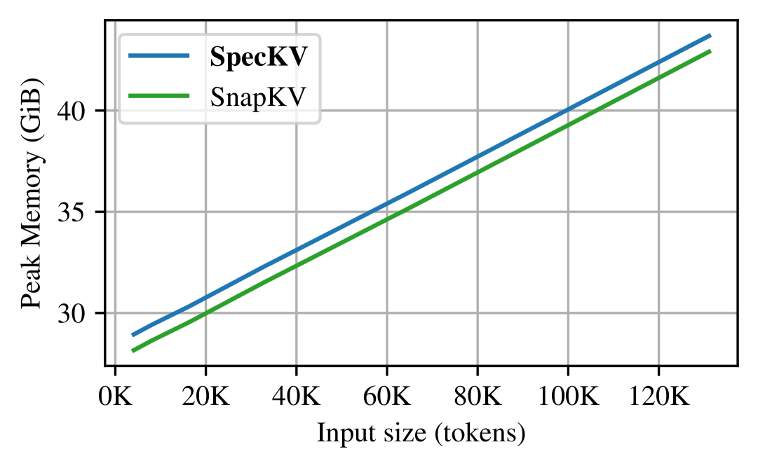
(a) KV dropping (${C_{\text{max}}}=256$), target model

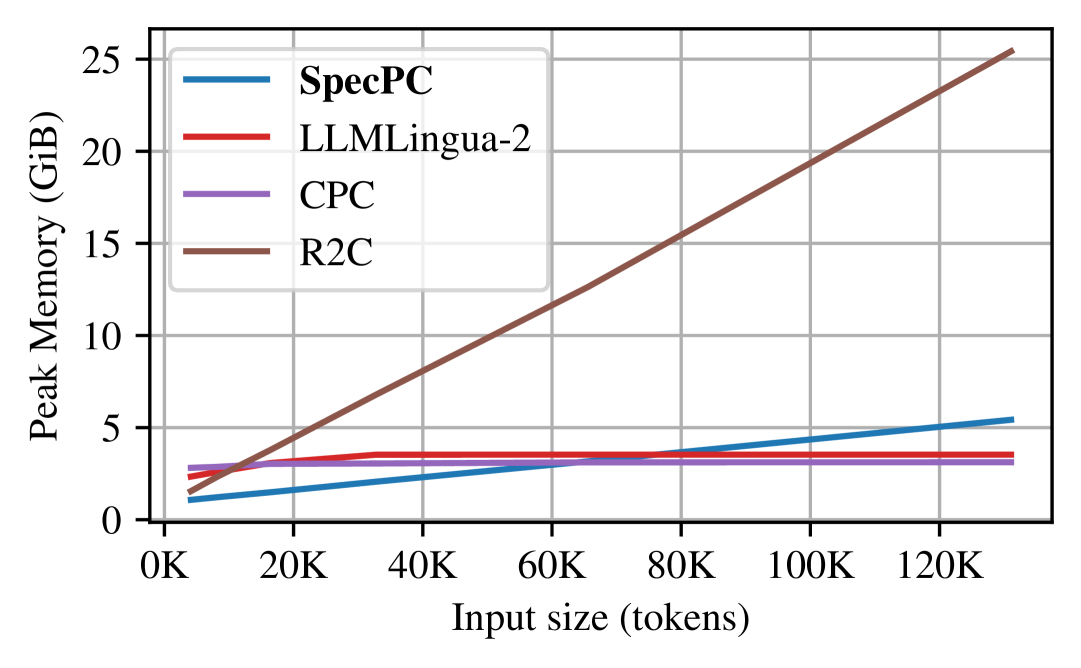
(b) Prompt compression (${C_{\text{max}}}=1024$), draft model

Figure 7: Peak memory usage.

Fig.˜7 compares the peak memory usage of KV dropping and prompt compression methods for Qwen2.5 (0.5B draft, 14B target). SpecKV consistently consumes more memory than SnapKV, primarily due to the need to load the draft model weights into memory. However, this additional overhead is constant and generally acceptable in practice. If further memory savings are required, it is possible to offload the draft model weights to the CPU.

For prompt compression, we compare the peak memory usage of the draft or auxiliary models, as the target model’s peak memory usage remains the same for a given ${C_{\text{max}}}$. The results indicate that SpecPC requires substantially less memory than R2C, the second-best performing method in our experiments, highlighting the efficiency advantage of our approach. For the remaining methods, SpecPC exhibits similar peak memory consumption.

E.2 Additional Attention Correlation Experiments

We present additional attention correlation plots in Fig.˜8 for Llama-3 [19], Qwen2.5 [51], Qwen3 [46], and Gemma-3 [45]. Across most model pairs, we observe strong correlations in attention patterns, especially when using mean aggregation for the attention activations.

E.3 Additional RULER and LongBench Results

Fig.˜9 (RULER), Tables˜9 and 10 (LongBench) present the performance of our proposed methods, SpecKV and SpecPC, alongside several baselines for additional values of ${C_{\text{max}}}$. While increasing the budget ${C_{\text{max}}}$ improves performance across all methods and narrows the gap between our approaches and the baselines, our proposed methods consistently outperform the alternatives.

E.4 MileBench (Multi-modal) Results

We conduct additional experiments using Qwen2.5-VL-3B-Instruct-AWQ (draft) and Qwen2.5-VL-32B-Instruct-AWQ (target) on six MileBench [14] datasets. We select three datasets each from the Temporal Multi-Image (EgocentricNavigation, MovingDirection, SceneTransition) and Semantic Multi-Image (SlideVQA, TQA, WebQA) categories. We focus on these datasets because, for Qwen2.5-VL, the performance gap between draft and target models is most significant; in other cases, the models perform too similarly or the draft even outperforms the target.

For KV dropping, we evaluate H20, SnapKV, and PyramidKV from our prior experiments. We do not include AdaKV in our evaluation as it is dependent on an older Transformers [49] version incompatible with Qwen2.5-VL. For prompt compression, we compare with FastV [10]—a method specialized for dropping image tokens inside LLMs—as techniques such as C2C and R2C do not support image inputs. FastV uses a hyperparameter $k$: it runs all tokens up to layer $k$, then drops less-attended image tokens based on the attention map, processing only the top tokens thereafter. This makes FastV less efficient than SpecPC, since all tokens must be processed up to $k$ with the full model, requiring considerable memory. Notably, FastV must compute the entire attention map at layer $k$, preventing the use of FlashAttention and leading to out-of-memory errors, even for moderate sequence lengths. As a result, many MileBench datasets exceed 80GB VRAM, so we limit our analysis to these six datasets.

Since the selected MileBench datasets have relatively short average context lengths, we conduct experiments using reduced ${C_{\text{max}}}$ values for both KV cache dropping (64, 96, and 128) and prompt compression (512, 768, and 1024).

Fig.˜10(a) presents results for various KV dropping methods. Our proposed method, SpecKV, demonstrates performance comparable to existing approaches, while significantly outperforming the others on the WebQA task.

Fig.˜10(b) compares the performance of SpecPC and FastV under two configurations ($k=2$ and $k=5$). Our method consistently outperforms FastV in most cases.

E.5 Ablation Studies

In this section, we conduct a series of ablation experiments to further analyze the effectiveness of our two proposed methods: SpecKV and SpecPC. For consistency, we fix ${C_{\text{max}}}$ to 256 for KV dropping and 1024 for prompt compression across all experiments. We utilize Qwen2.5 (Instruct), employing the 0.5B model as the draft and the 14B model as the target. We sample 100 random examples per task from the LongBench and RULER benchmarks.

E.5.1 SpecKV: Leveraging Enhanced Draft Models

Fig.˜11 illustrates the impact of using draft models of different sizes and versions on the RULER score. As anticipated, both newer [46] and larger draft models lead to improved performance of SpecKV.

E.5.2 SpecKV and SpecPC: Number of Generated Draft Tokens

Fig.˜12 illustrates how varying the number of generated draft tokens, ${n_{\text{lookahead}}}$, affects the performance of SpecKV and SpecPC. Overall, increasing ${n_{\text{lookahead}}}$ generally results in higher final accuracy for SpecKV, whereas it yields only marginal improvements for SpecPC. We attribute this to the larger ${C_{\text{max}}}$ budget of SpecPC, which allows it to capture all important tokens without needing to generate long drafts.

E.5.3 SpecKV: Accuracy Impact of Sparse Prefill

In this section, we experimentally evaluate how the sparsity of SpecKV’s prefill procedure affects downstream task performance (Fig.˜13). Specifically, we set ${n_{\text{vert}}}$ equal to ${n_{\text{slash}}}$ and compare several values for these parameters. As anticipated, reducing sparsity (i.e., using a higher ${n_{\text{vert}}}$) generally results in higher accuracy; however, accuracy improvements plateau at ${n_{\text{vert}}}=2048$, which we therefore adopt for our main experiments.

Interestingly, for certain LongBench categories, increased sparsity (i.e., lower ${n_{\text{vert}}}$) can actually lead to improved performance. This counterintuitive result suggests that, for some tasks, sparser prefill may serve as a form of regularization, preventing overfitting to irrelevant context.

E.6 Additional Models

In this section, we present results for RULER and LongBench using larger models. Specifically, we employ Qwen2.5-32B-Instruct, Qwen2.5-72B-Instruct-GPTQ-Int4, and Llama-3.1-70B-Instruct (4-bit quantized with bitsandbytes) as target model. To explore the impact of draft model size in SpecKV, we extend our experiments to larger drafts—Qwen2.5-1.5B-Instruct, Qwen2.5-3B-Instruct, and Llama-3.2-3B-Instruct—in addition to the previously used Qwen2.5-0.5B-Instruct and Llama-3.2-1B-Instruct. This enables us to systematically examine how increasing the draft size improves performance. For SpecPC, we find Qwen2.5-0.5B-Instruct and Llama-3.2-1B-Instruct already deliver sufficient performance.

For each RULER and LongBench task, we randomly select 50 samples and compare SpecKV to SnapKV, as well as SpecPC to CPC and R2C—the best-performing methods in our previous experiments. For ${C_{\text{max}}}$, we use values of 256, 512, and 1024 for KV dropping, and 1024, 2048, and 3072 for prompt compression.

Figs.˜14 and 15 show the RULER results, and Tables˜11, 12 and 13 present the LongBench results. Overall, our method achieves higher accuracy than the baselines in most settings, especially with small ${C_{\text{max}}}$. Specifically, SpecKV significantly outperforms SnapKV on RULER, with performance further improved by utilizing a larger draft model. Similarly, SpecPC consistently achieves strong results, particularly at longer sequence lengths on RULER. On LongBench, both of our methods also surpass the baselines.

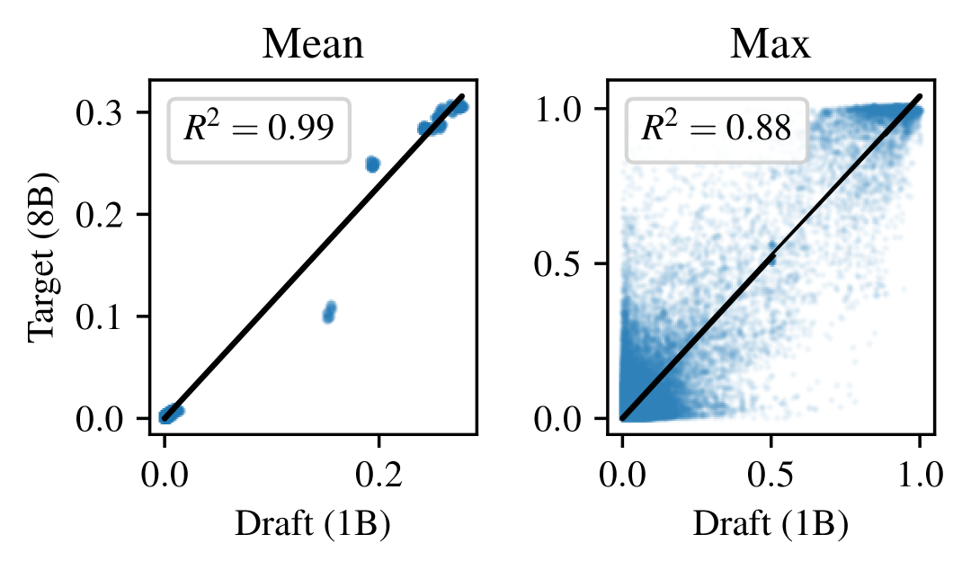
(a) Llama-3 (1B / 8B)

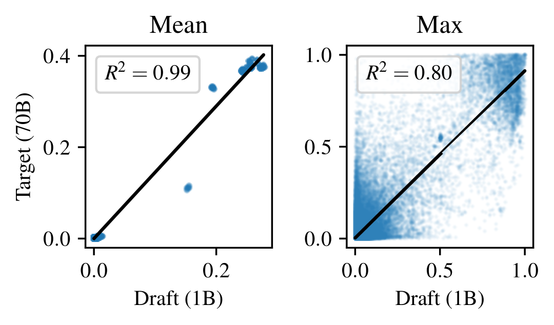
(b) Llama-3 (1B / 70B)

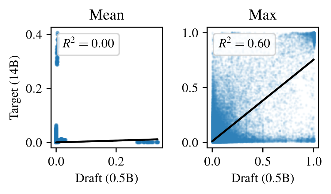
(c) Qwen2.5 (0.5B / 14B)

(d) Qwen2.5 (0.5B / 72B)

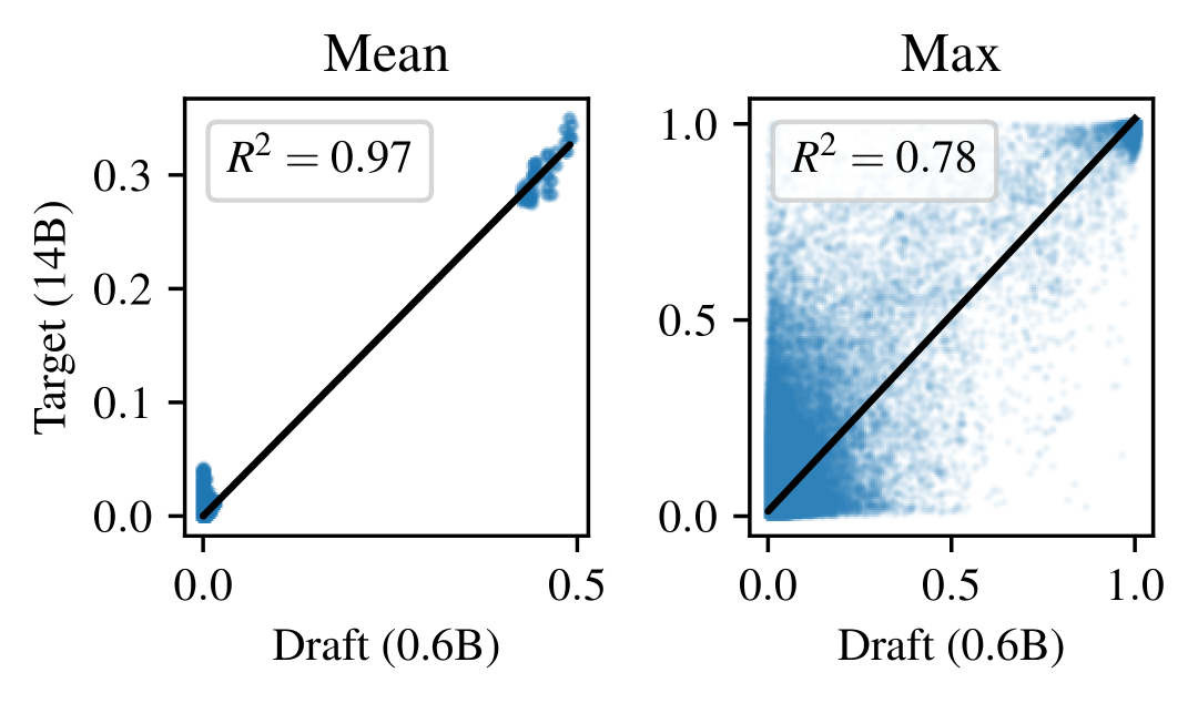
(e) Qwen3 (0.6B / 14B)

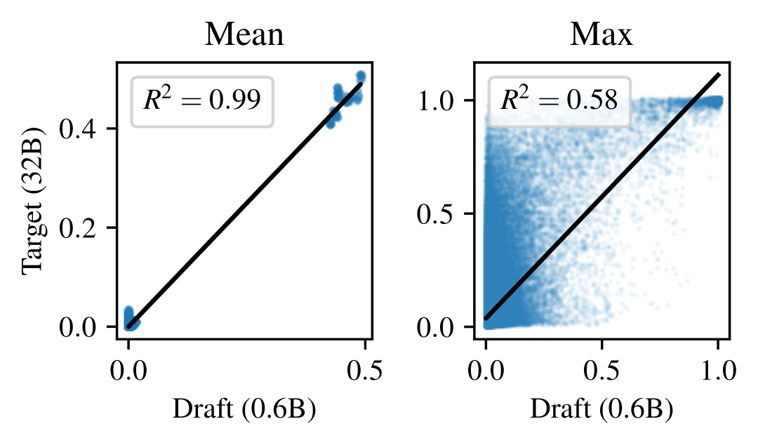
(f) Qwen3 (0.6B / 32B)

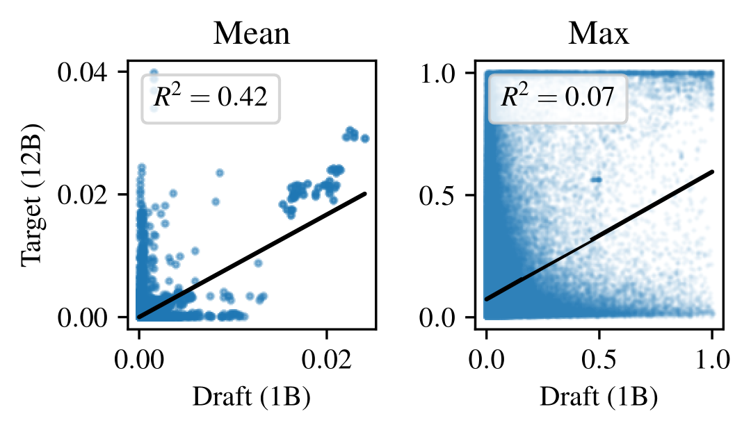
(g) Gemma-3 (1B / 12B)

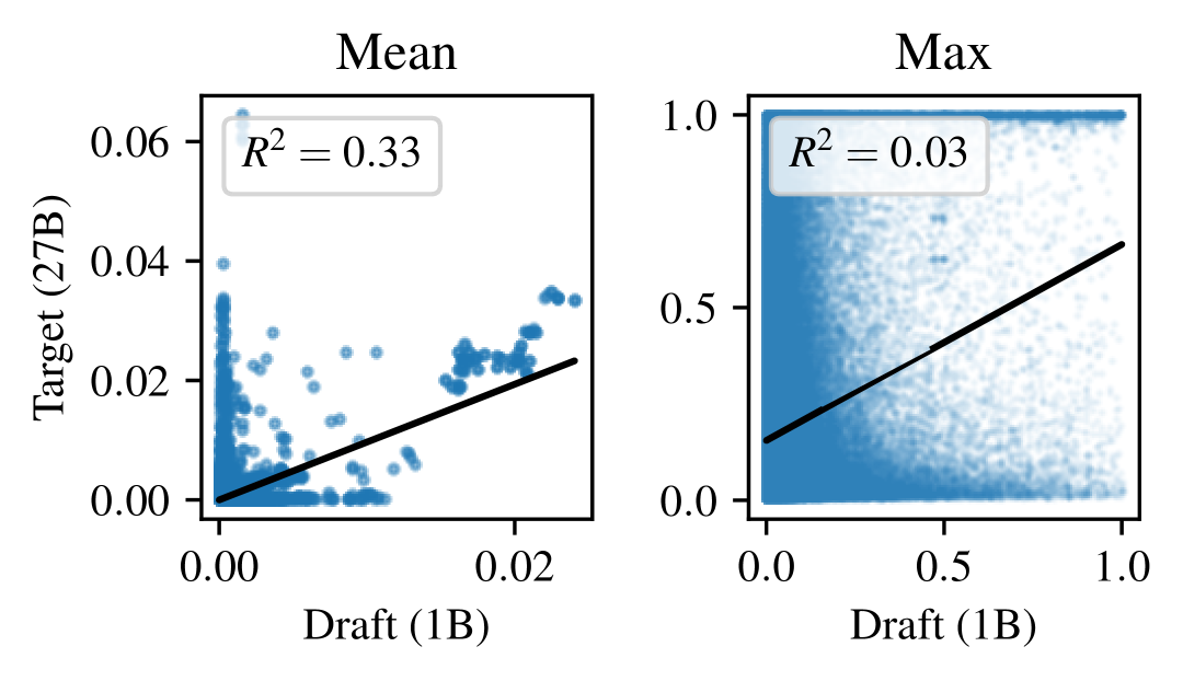
(h) Gemma-3 (1B / 27B)

Figure 8: Additional attention correlation plots for mean and max aggregation across different model combinations. Blue dots indicate attention activation pairs for draft and target; the black line represents the best linear fit. We observe strong correlations in most cases, especially with mean aggregation—even between models with large size gaps, such as Qwen2.5 (0.5B/72B). Correlation is notably weaker for Qwen2.5 (0.5B/14B), yet our methods still perform robustly on this model.

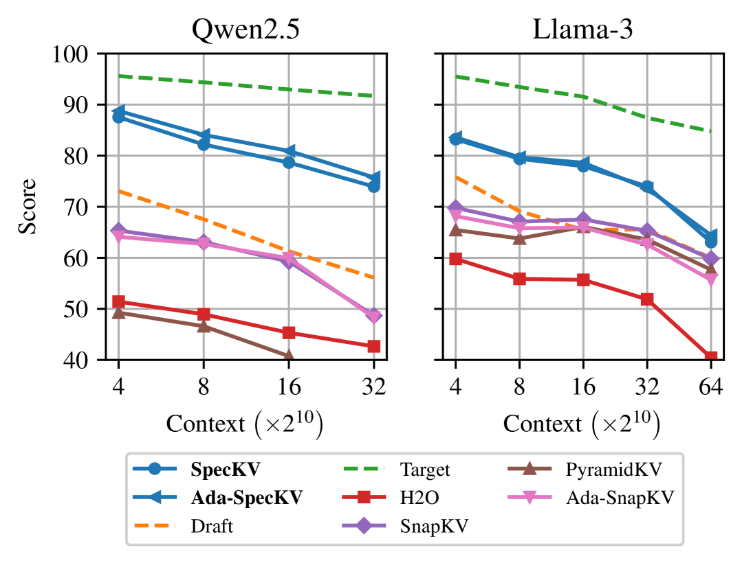
(a) KV dropping (${C_{\text{max}}}=256$)

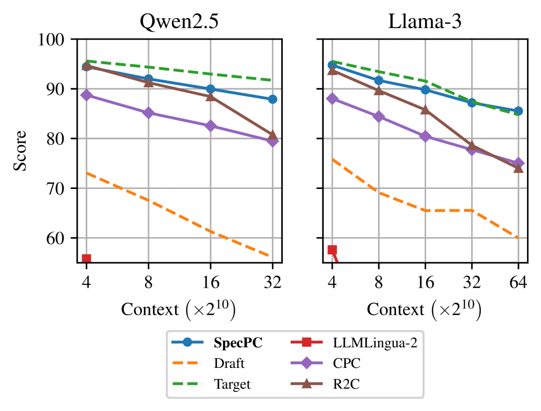
(b) Prompt compression (${C_{\text{max}}}=1024$)

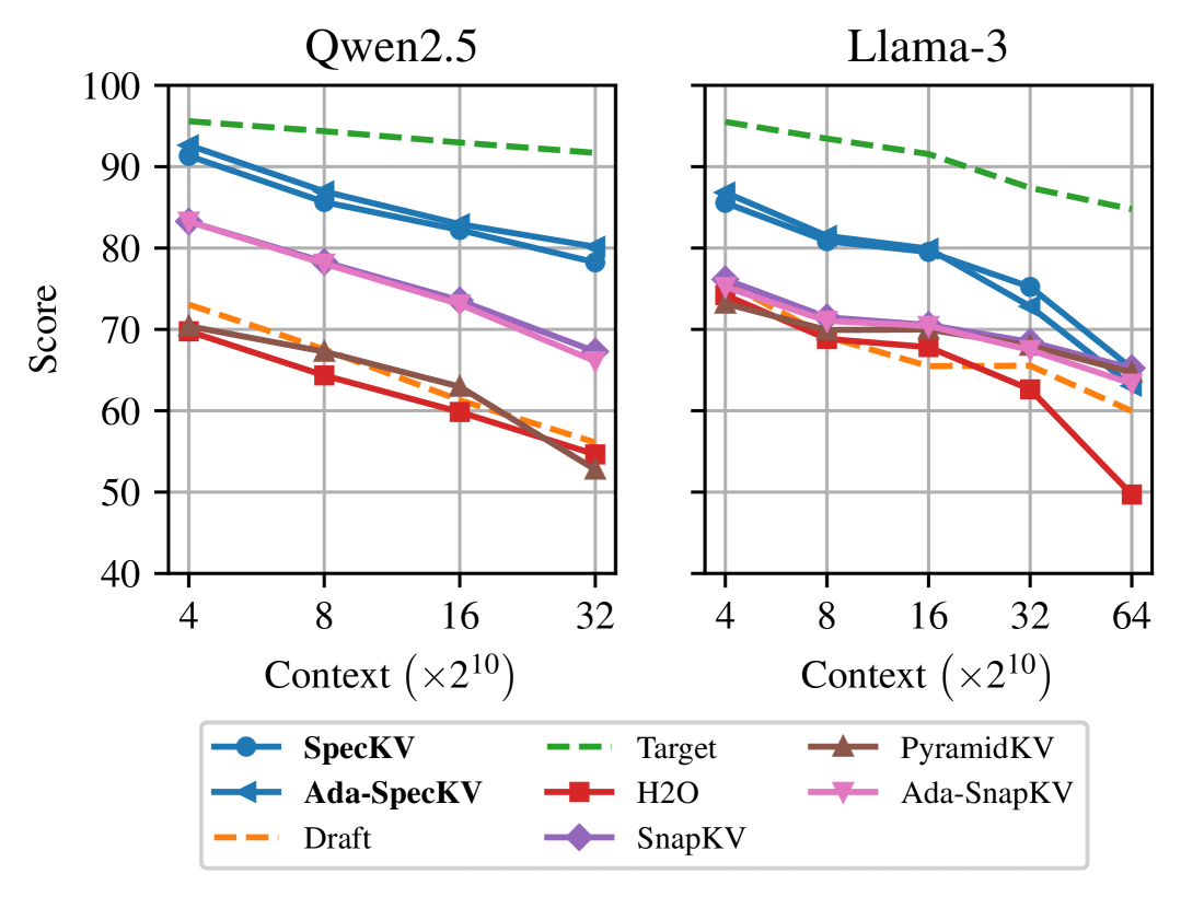
(c) KV dropping (${C_{\text{max}}}=512$)

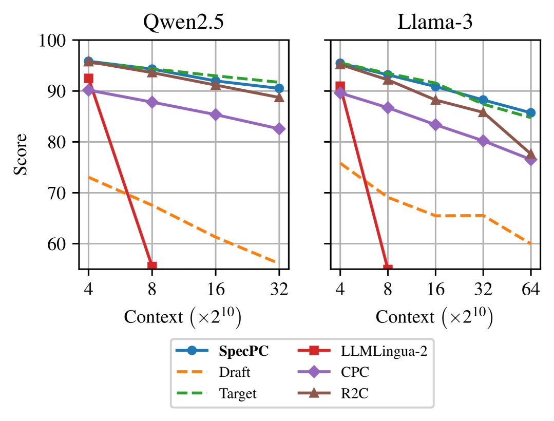
(d) Prompt compression (${C_{\text{max}}}=2048$)

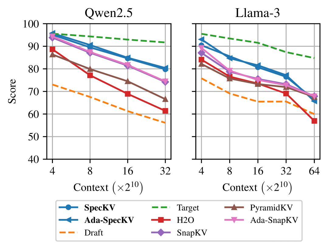
(e) KV dropping (${C_{\text{max}}}=1024$)

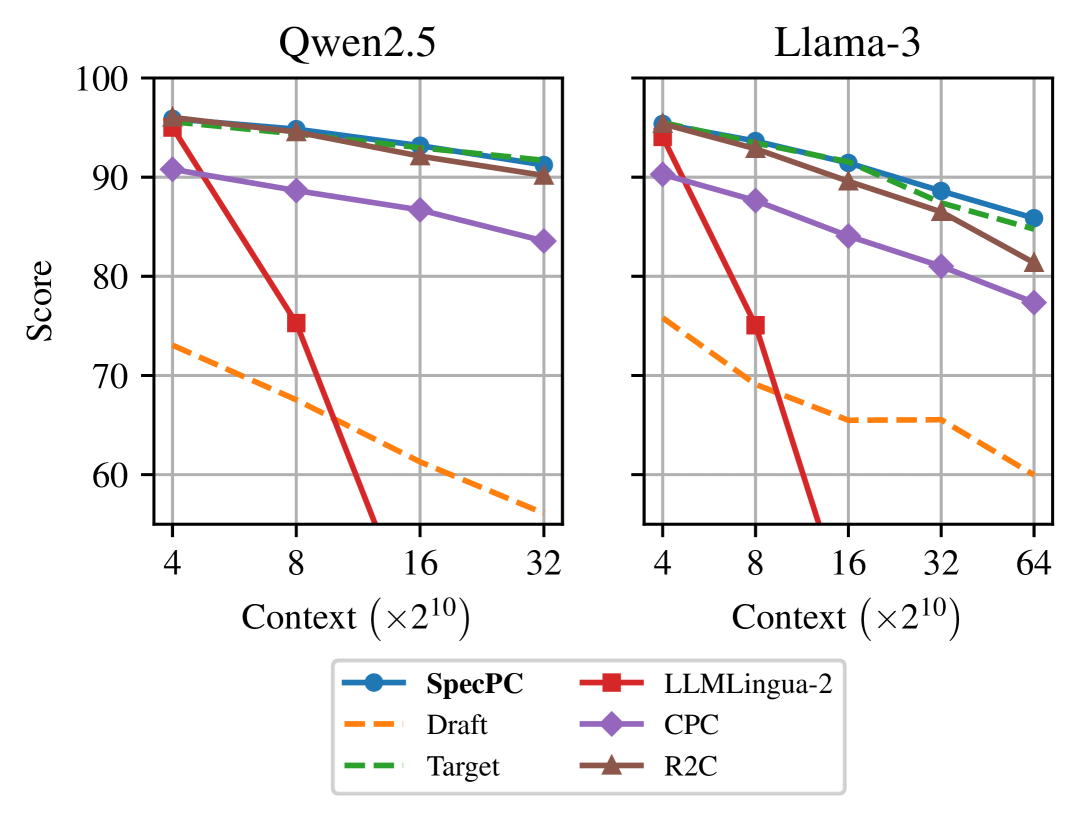
(f) Prompt compression (${C_{\text{max}}}=3072$)

Figure 9: Performance of the proposed SpecKV and SpecPC on RULER compared to various baselines (full results), using Qwen2.5-0.5B-Instruct and Llama-3.2-1B-Instruct as draft models, and Qwen2.5-14B-Instruct and Llama-3.1-8B-Instruct as target models. Our approaches consistently outperform all baselines across every sequence length. Notably, SpecPC performs nearly on par with the target model. Low-performing methods are omitted.

Table 9: Full results for LongBench performance with Qwen2.5-0.5B (draft) and Qwen2.5-14B (target).

	${C_{\text{max}}}$	Method	Single- doc QA	Multi- doc QA	Summary	Few-shot Learning	Code Completion	All
Dense	–	Draft	21.04	24.4	21.23	54.07	33.39	30.64
		Target	53.19	42.83	24.99	65.34	51.75	47.33
KV	256	StreamingLLM	38.66	24.13	19.10	49.75	35.23	33.24
		H2O	46.98	29.66	19.82	50.88	47.86	38.41
		SnapKV	49.07	33.19	19.49	54.49	47.34	40.25
		PyramidKV	47.07	31.84	18.32	54.81	43.26	38.76
		Ada-SnapKV	50.92	34.57	19.63	55.07	49.58	41.41
		SpecKV	51.07	38.76	23.20	59.68	49.58	44.09
		Ada-SpecKV	51.92	39.38	24.90	61.05	53.43	45.61
	512	StreamingLLM	38.97	27.04	21.14	53.78	36.52	35.41
		H2O	47.56	33.16	21.02	53.45	49.78	40.37
		SnapKV	50.74	38.33	20.97	57.81	49.94	43.10
		PyramidKV	50.19	36.37	20.25	58.17	47.88	42.19
		Ada-SnapKV	51.69	38.61	21.48	59.84	51.85	44.18
		SpecKV	51.98	41.51	24.11	62.60	52.33	46.09
		Ada-SpecKV	51.00	42.18	25.74	63.74	55.28	48.46
	1024	StreamingLLM	40.08	32.01	22.12	55.42	38.36	37.54
		H2O	49.73	37.27	22.38	55.94	51.26	42.75
		SnapKV	51.56	40.98	22.65	63.90	51.48	45.73
		PyramidKV	51.42	40.93	21.76	59.96	49.92	44.43
		Ada-SnapKV	51.81	40.96	22.83	64.14	51.97	45.94
		SpecKV	52.92	41.85	24.30	63.46	52.50	46.61
		Ada-SpecKV	52.27	43.22	26.39	64.83	54.40	47.78
PC	1024	LLMLingua-2	27.10	23.74	22.57	35.85	37.62	28.79
		CPC	42.76	36.05	22.58	48.38	35.57	37.17
		R2C	46.43	37.42	22.64	47.21	29.48	37.15
		SpecPC	47.70	38.30	23.30	59.74	52.52	43.73
	2048	LLMLingua-2	35.10	32.22	23.51	39.82	44.80	34.40
		CPC	48.74	39.70	23.39	55.77	42.07	41.92
		R2C	50.68	40.65	23.47	56.72	45.62	43.27
		SpecPC	53.23	41.43	23.68	63.26	54.92	46.76
	3072	LLMLingua-2	43.50	35.67	24.10	45.66	47.32	38.67
		CPC	51.59	41.08	23.84	58.14	44.82	43.83
		R2C	51.71	41.39	23.89	62.09	48.58	45.31
		SpecPC	53.25	41.48	24.49	64.51	54.41	47.14

Table 10: Full results for LongBench performance with Llama-3.2-1B (draft) and Llama-3.1-8B (target).

	${C_{\text{max}}}$	Method	Single- doc QA	Multi- doc QA	Summary	Few-shot Learning	Code Completion	All
Dense	–	Draft	28.08	27.27	25.65	60.16	31.11	34.69
		Target	45.85	43.79	28.68	66.65	50.46	46.84
KV	256	StreamingLLM	38.69	27.12	21.64	50.75	34.74	34.58
		H2O	43.54	36.81	22.62	55.64	47.81	40.82
		SnapKV	43.79	37.31	21.96	56.29	47.34	40.91
		PyramidKV	43.62	37.79	21.75	55.15	46.32	40.54
		Ada-SnapKV	44.04	37.86	22.34	59.95	50.39	42.38
		SpecKV	43.23	39.73	24.43	60.90	51.09	43.36
		Ada-SpecKV	42.40	40.73	25.74	57.94	52.51	43.25
	512	StreamingLLM	38.80	29.15	24.16	52.59	37.25	36.33
		H2O	44.82	39.36	23.95	58.70	49.30	42.79
		SnapKV	45.00	41.31	23.61	61.36	49.92	43.83
		PyramidKV	45.26	41.22	23.36	61.15	48.06	43.51
		Ada-SnapKV	45.09	41.17	24.19	61.81	51.74	44.30
		SpecKV	43.48	41.86	26.17	62.34	51.36	44.59
		Ada-SpecKV	43.80	42.56	26.59	58.72	54.41	44.56
	1024	StreamingLLM	38.45	32.54	25.03	58.09	38.60	38.54
		H2O	45.45	42.50	25.42	59.17	50.10	44.13
		SnapKV	45.46	43.15	25.42	62.06	52.37	45.22
		PyramidKV	46.10	42.78	25.17	63.43	49.55	45.11
		Ada-SnapKV	46.06	43.34	25.48	63.47	50.50	45.43
		SpecKV	43.73	43.39	26.95	63.14	51.28	45.30
		Ada-SpecKV	44.83	43.72	27.50	61.04	54.23	45.70
PC	1024	LLMLingua-2	29.61	24.83	23.43	24.18	40.66	27.68
		CPC	35.67	36.61	25.26	34.01	43.58	34.42
		R2C	38.41	39.07	25.28	43.26	43.99	37.58
		SpecPC	44.83	39.94	25.85	63.70	44.82	43.76
	2048	LLMLingua-2	34.00	32.51	24.90	24.76	47.27	31.64
		CPC	40.02	39.41	26.83	39.02	46.66	37.80
		R2C	44.53	38.97	26.63	54.62	46.67	41.97
		SpecPC	44.92	40.71	27.30	64.77	46.89	44.78
	3072	LLMLingua-2	39.13	35.44	25.98	29.73	49.92	35.05
		CPC	41.73	39.52	27.27	42.12	49.13	39.30
		R2C	44.77	40.97	27.35	60.85	48.08	44.14
		SpecPC	47.12	41.95	28.02	65.61	45.52	45.65

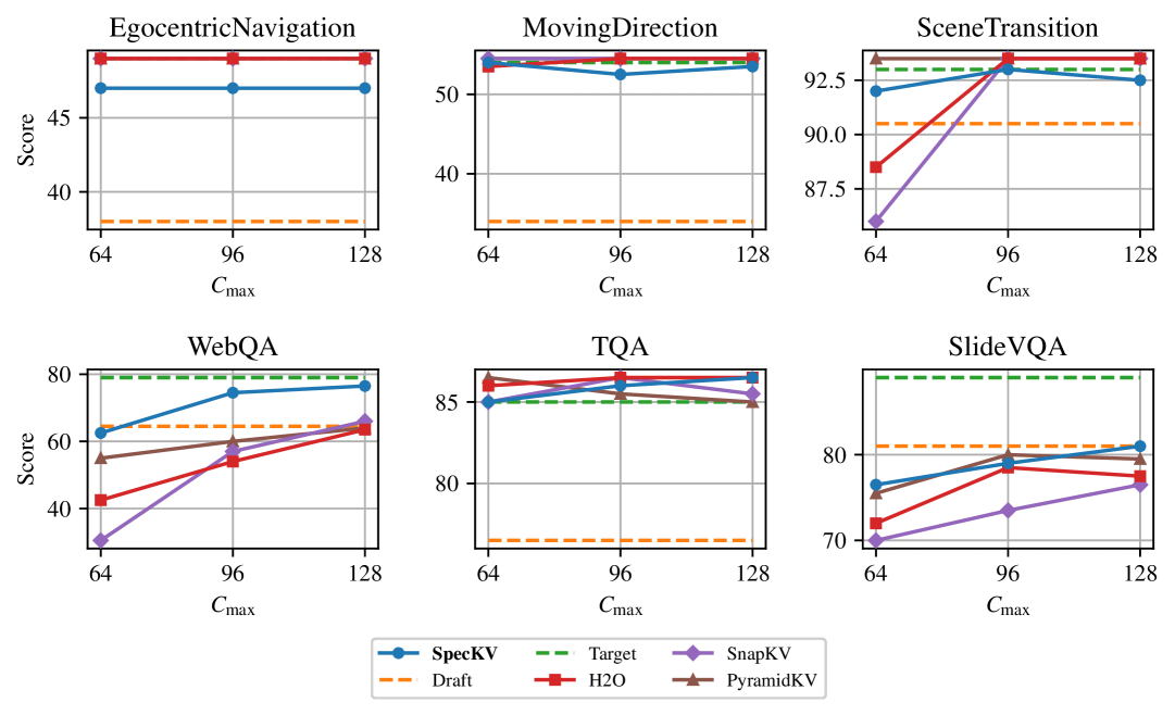
(a) KV dropping

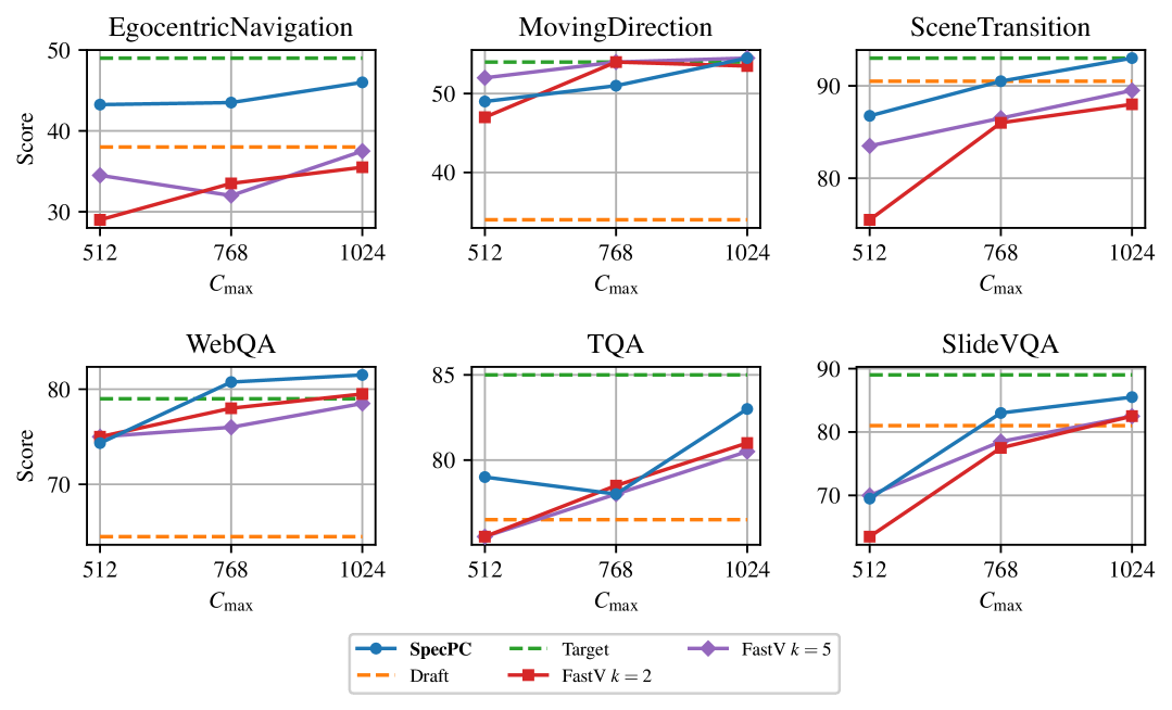
(b) Prompt compression

Figure 10: MileBench multi-modal results using Qwen2.5-VL-3B-Instruct-AWQ (draft) and Qwen2.5-VL-32B-Instruct-AWQ (target). SpecKV demonstrates competitive performance across most tasks and achieves a substantial improvement on WebQA. SpecPC consistently outperforms both FastV configurations on the majority of datasets.

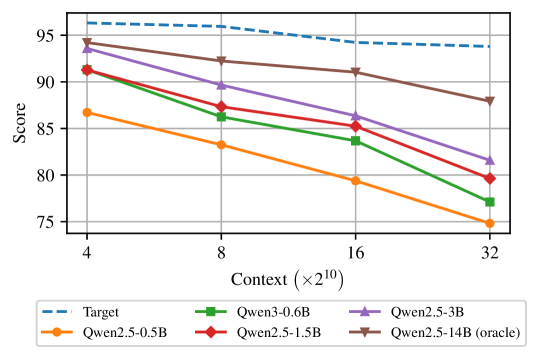
Figure 11: Effect of draft model quality on RULER score. The target model is Qwen2.5-14B (Instruct). Consistent with expectations, employing more capable draft models boosts performance. For reference, we also evaluate an oracle setting where the draft model is identical to the target (Qwen2.5-14B), representing an empirical upper bound for SpecKV.

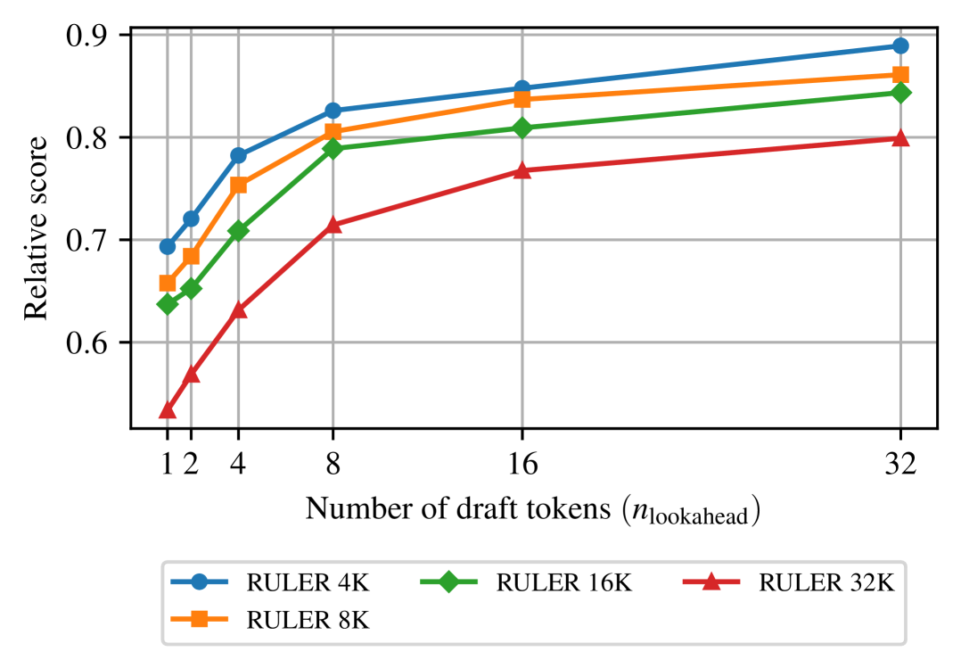
(a) SpecKV on RULER

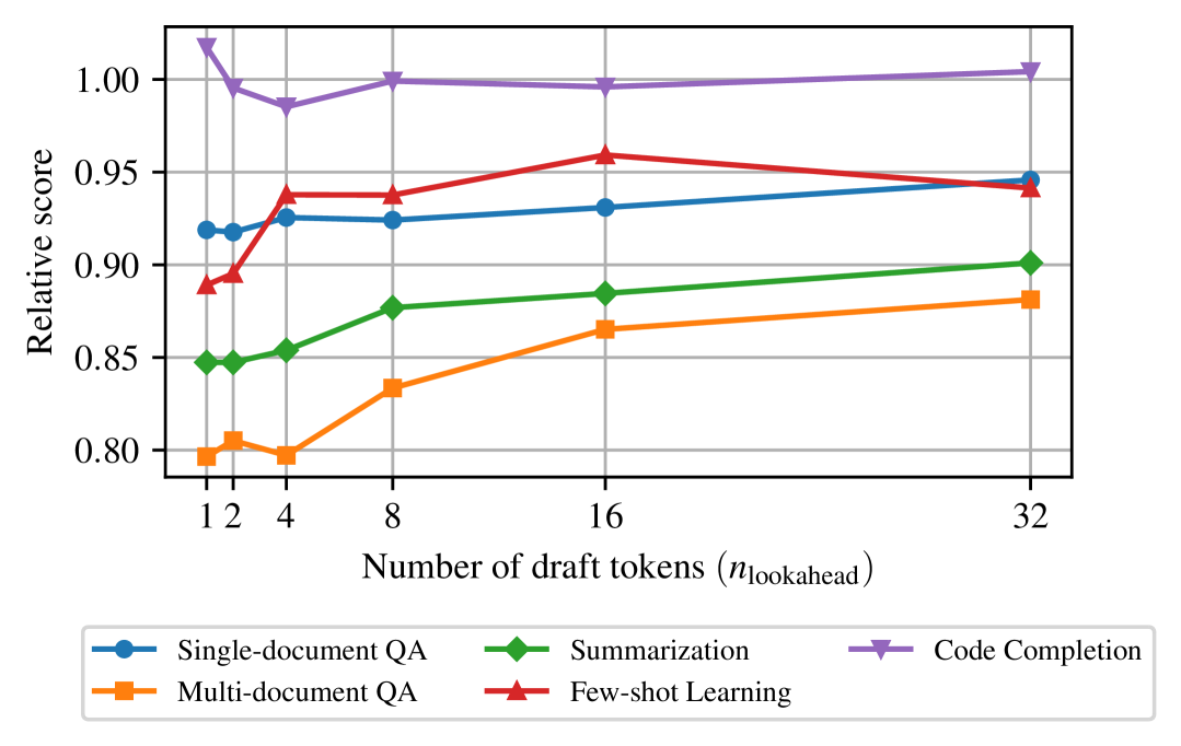
(b) SpecKV on LongBench

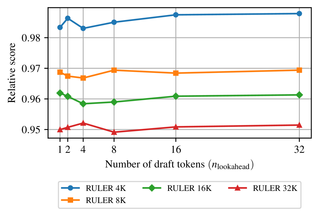
(c) SpecPC on RULER

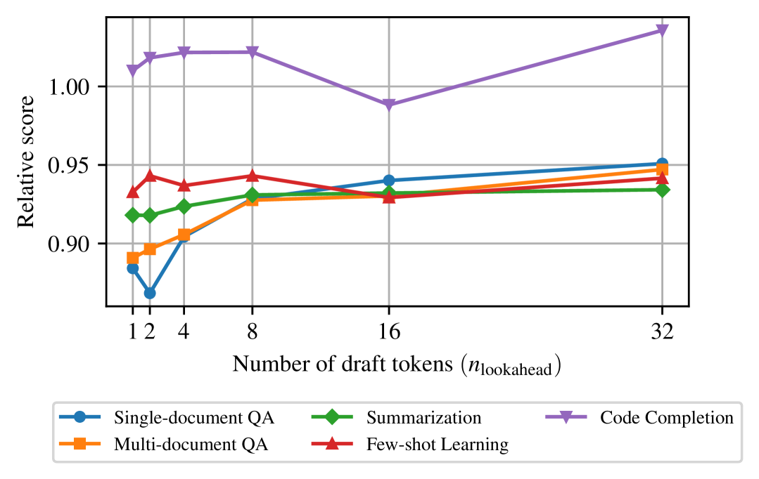
(d) SpecPC on LongBench

Figure 12: Impact of the number of generated draft tokens, ${n_{\text{lookahead}}}$, on the relative performance of SpecKV and SpecPC, using Qwen2.5-0.5B-Instruct as the draft model and Qwen2.5-14B-Instruct as the target model. The relative score is calculated as the score of each SpecKV configuration divided by the score of the full dense target model. Increasing ${n_{\text{lookahead}}}$ substantially boosts SpecKV’s score, whereas SpecPC shows only minor improvement with higher ${n_{\text{lookahead}}}$.

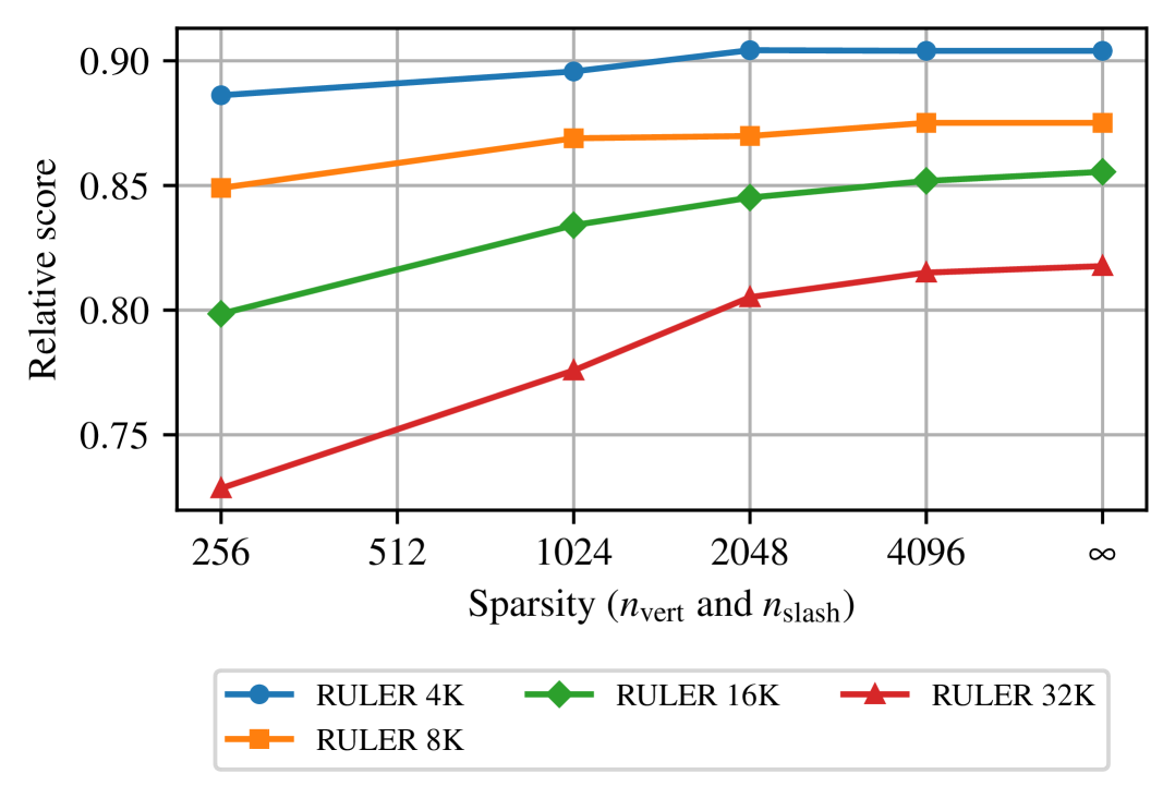
(a) RULER

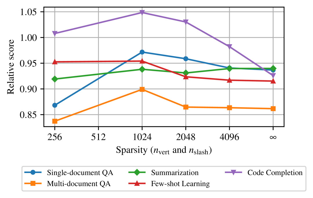
(b) LongBench

Figure 13: Impact of different sparsity levels in SpecKV’s sparse prefill on relative performance, using Qwen2.5-0.5B-Instruct as the draft model and Qwen2.5-14B-Instruct as the target model. We vary ${n_{\text{vert}}}$ (set equal to ${n_{\text{slash}}}$) and observe the impact on accuracy. Accuracy improves as sparsity decreases (higher ${n_{\text{vert}}}$) up to 2048, beyond which gains saturate, hence our choice of 2048 for main results. $\infty$ corresponds to fully dense prefill. Notably, for some LongBench tasks, higher sparsity actually benefits accuracy. The relative score is calculated as the score of each SpecKV configuration divided by the score of the full dense target model.

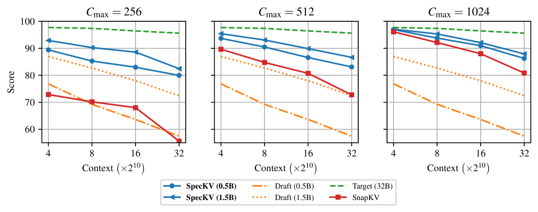
(a) Qwen2.5: Draft models (0.5B, 1.5B), target model (32B)

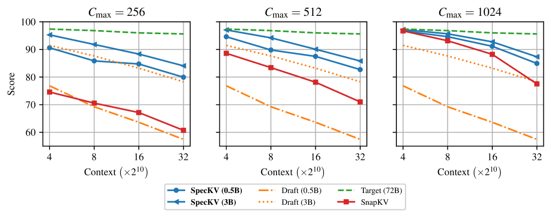
(b) Qwen2.5: Draft models (0.5B, 3B), target model (72B, 4-bit)

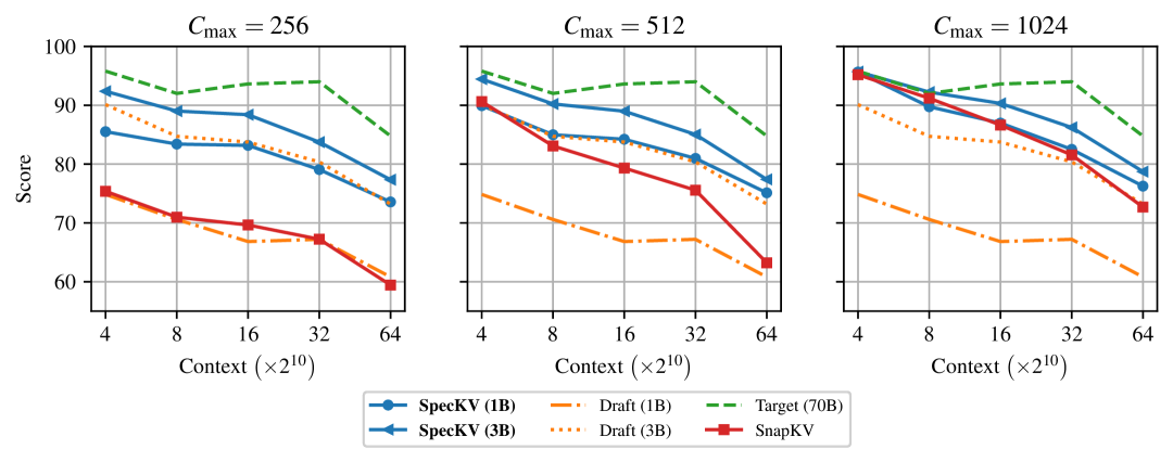
(c) Llama-3: Draft models (3.2-1B, 3.2-3B), target model (3.1-70B, 4-bit)

Figure 14: RULER results of additional larger models on KV cache dropping. Our proposed SpecKV method consistently outperforms SnapKV across the majority of evaluated settings, often by a substantial margin. Utilizing a larger draft model leads to further performance improvements.

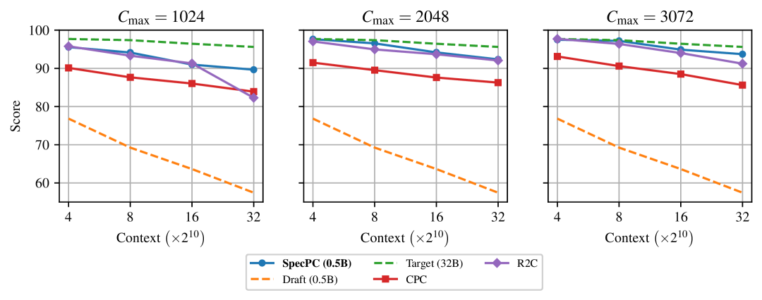
(a) Qwen2.5: Draft model (0.5B), target model (32B)

(b) Qwen2.5: Draft model (0.5B), target model (72B, 4-bit)

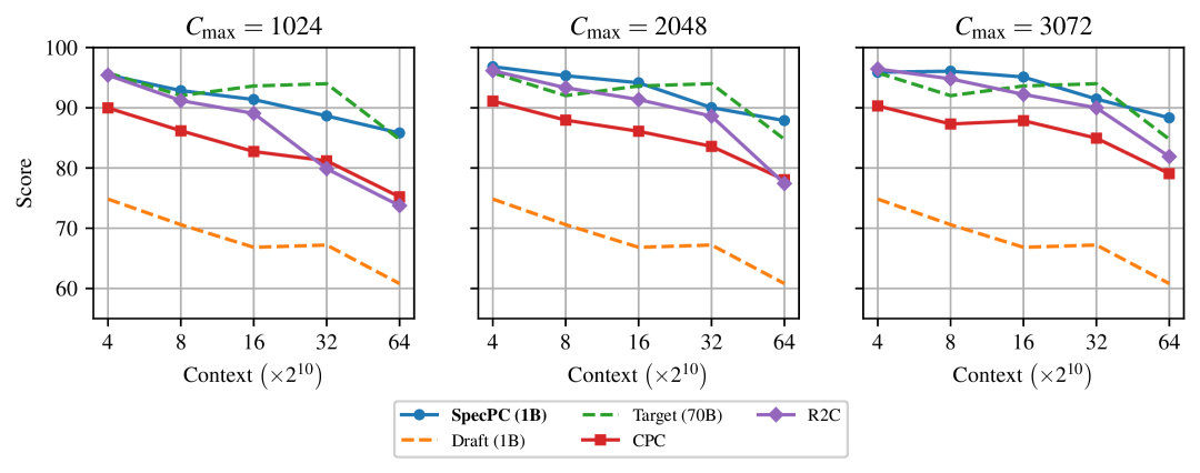
(c) Llama-3: Draft model (3.2-1B), target model (3.1-70B, 4-bit)

Figure 15: RULER results of additional larger models on prompt compression. Our proposed SpecPC method consistently outperforms CPC and R2C, maintaining strong performance even on long sequences.

Table 11: LongBench results for Qwen2.5, featuring 0.5B and 1.5B draft models and a 32B target model.

	${C_{\text{max}}}$	Method	Single- doc QA	Multi- doc QA	Summary	Few-shot Learning	Code Completion	All
Dense	–	Draft (0.5B)	19.07	26.58	20.90	53.51	32.48	30.37
		Draft (1.5B)	36.16	35.01	22.79	63.92	36.62	39.06
		Target (32B)	56.01	43.99	25.90	64.06	44.74	47.78
KV	256	SnapKV	52.54	40.21	19.89	61.18	40.12	42.98
		SpecKV (0.5B)	52.45	42.12	23.10	63.55	45.72	45.36
		SpecKV (1.5B)	53.48	43.77	24.02	63.79	44.80	46.06
	512	SnapKV	55.24	42.21	21.47	63.36	39.69	44.73
		SpecKV (0.5B)	53.70	42.70	24.16	63.68	43.14	45.64
		SpecKV (1.5B)	52.78	43.97	24.80	64.72	46.77	46.60
	1024	SnapKV	55.32	44.04	23.08	66.15	44.42	46.76
		SpecKV (0.5B)	57.56	43.67	24.62	65.68	42.25	47.08
		SpecKV (1.5B)	55.72	43.95	25.20	63.31	42.38	46.38
PC	1024	CPC	45.60	40.62	23.09	60.08	32.31	40.91
		R2C	50.49	40.37	23.26	53.45	34.11	39.88
		SpecPC (0.5B)	51.23	41.40	23.37	62.26	38.23	43.66
	2048	CPC	51.01	42.31	23.74	60.92	35.83	43.26
		R2C	50.32	42.66	24.08	59.11	40.54	44.19
		SpecPC (0.5B)	55.40	42.60	24.12	61.46	48.05	46.20
	3072	CPC	56.80	42.05	24.77	62.79	37.98	45.37
		R2C	51.67	42.88	24.09	62.45	27.01	42.66
		SpecPC (0.5B)	56.89	42.42	24.71	62.66	47.49	46.79

Table 12: LongBench results for Qwen2.5, featuring 0.5B and 3B draft models and a 72B (4-bit) target model.

	${C_{\text{max}}}$	Method	Single- doc QA	Multi- doc QA	Summary	Few-shot Learning	Code Completion	All
Dense	–	Draft (0.5B)	19.07	26.58	20.90	53.51	32.48	30.37
		Draft (3B)	39.26	40.06	25.34	63.43	45.31	42.49
		Target (72B)	58.70	45.89	26.24	64.83	51.08	49.22
KV	256	SnapKV	55.85	40.12	21.65	55.82	50.41	44.37
		SpecKV (0.5B)	54.11	42.13	24.28	64.72	47.82	46.53
		SpecKV (3B)	53.05	44.49	24.94	63.09	48.48	46.69
	512	SnapKV	59.08	44.13	23.04	61.33	51.77	47.59
		SpecKV (0.5B)	54.00	45.08	25.26	64.40	47.39	47.22
		SpecKV (3B)	56.99	45.31	25.83	61.66	48.46	47.59
	1024	SnapKV	59.56	44.06	24.41	62.85	52.87	48.46
		SpecKV (0.5B)	56.58	44.70	25.45	61.95	49.59	47.52
		SpecKV (3B)	58.14	44.69	26.36	61.81	50.53	48.15
PC	1024	CPC	46.37	38.36	24.19	52.54	28.30	38.64
		R2C	55.78	40.10	24.40	47.62	33.17	40.72
		SpecPC (0.5B)	48.52	45.34	24.14	61.04	48.30	45.26
	2048	CPC	55.14	43.53	24.71	49.46	33.21	41.78
		R2C	54.61	45.70	24.99	53.65	42.43	44.41
		SpecPC (0.5B)	58.36	46.38	25.32	64.43	51.11	48.98
	3072	CPC	55.78	44.41	25.47	42.71	39.16	41.68
		R2C	59.22	44.70	25.69	55.22	44.04	45.90
		SpecPC (0.5B)	59.84	44.95	25.91	64.18	46.88	48.46

Table 13: LongBench results for Llama-3, featuring 3.2-1B and 3.2-3B draft models and a 3.1-70B (4-bit) target model.

	${C_{\text{max}}}$	Method	Single- doc QA	Multi- doc QA	Summary	Few-shot Learning	Code Completion	All
Dense	–	Draft (1B)	28.37	28.62	26.12	59.10	33.59	35.27
		Draft (3B)	45.53	40.52	27.46	64.82	46.73	44.89
		Target (70B)	55.02	47.06	28.61	70.47	48.19	49.99
KV	256	SnapKV	55.88	45.30	22.49	62.15	55.49	47.75
		SpecKV (1B)	52.03	46.51	25.35	62.00	56.59	47.91
		SpecKV (3B)	51.80	47.23	25.53	64.02	58.75	48.80
	512	SnapKV	56.08	46.94	24.40	63.34	52.14	48.32
		SpecKV (1B)	52.06	47.78	26.73	65.40	54.77	48.96
		SpecKV (3B)	53.31	47.47	27.33	67.49	54.19	49.66
	1024	SnapKV	54.94	47.40	25.97	67.56	48.13	48.85
		SpecKV (1B)	51.32	48.48	27.31	67.12	50.69	48.86
		SpecKV (3B)	53.32	46.02	27.41	66.40	50.66	48.63
PC	1024	CPC	45.14	39.41	24.86	61.40	37.58	41.97
		R2C	48.93	42.01	25.38	58.91	40.19	43.29
		SpecPC (1B)	56.84	44.48	25.91	67.37	47.15	48.44
	2048	CPC	55.97	46.00	26.72	64.78	41.31	47.36
		R2C	53.62	46.70	26.27	62.41	47.90	47.34
		SpecPC (1B)	59.39	46.25	27.60	68.42	46.70	49.88
	3072	CPC	56.64	46.69	27.29	64.92	44.75	48.30
		R2C	56.11	45.15	27.51	61.76	47.17	47.57
		SpecPC (1B)	58.47	48.07	27.72	65.43	41.28	48.69

References

- [1] Josh Achiam, Steven Adler, Sandhini Agarwal, Lama Ahmad, Ilge Akkaya, Florencia Leoni Aleman, Diogo Almeida, Janko Altenschmidt, Sam Altman, Shyamal Anadkat, et al. Gpt-4 technical report. arXiv preprint arXiv:2303.08774, 2023.
- [2] Joshua Ainslie, James Lee-Thorp, Michiel de Jong, Yury Zemlyanskiy, Federico Lebron, and Sumit Sanghai. Gqa: Training generalized multi-query transformer models from multi-head checkpoints. In Proceedings of the 2023 Conference on Empirical Methods in Natural Language Processing, pages 4895–4901, 2023.
- [3] Shuai Bai, Keqin Chen, Xuejing Liu, Jialin Wang, Wenbin Ge, Sibo Song, Kai Dang, Peng Wang, Shijie Wang, Jun Tang, et al. Qwen2. 5-vl technical report. arXiv preprint arXiv:2502.13923, 2025.
- [4] Yushi Bai, Xin Lv, Jiajie Zhang, Hongchang Lyu, Jiankai Tang, Zhidian Huang, Zhengxiao Du, Xiao Liu, Aohan Zeng, Lei Hou, Yuxiao Dong, Jie Tang, and Juanzi Li. LongBench: A bilingual, multitask benchmark for long context understanding. In Proceedings of the 62nd Annual Meeting of the Association for Computational Linguistics (Volume 1: Long Papers), pages 3119–3137, Bangkok, Thailand, August 2024. Association for Computational Linguistics.
- [5] Iz Beltagy, Matthew E. Peters, and Arman Cohan. Longformer: The long-document transformer. arXiv:2004.05150, 2020.
- [6] Tianle Cai, Yuhong Li, Zhengyang Geng, Hongwu Peng, Jason D Lee, Deming Chen, and Tri Dao. Medusa: Simple llm inference acceleration framework with multiple decoding heads. In International Conference on Machine Learning, pages 5209–5235. PMLR, 2024.
- [7] Zefan Cai, Yichi Zhang, Bofei Gao, Yuliang Liu, Tianyu Liu, Keming Lu, Wayne Xiong, Yue Dong, Baobao Chang, Junjie Hu, and Xiao Wen. Pyramidkv: Dynamic kv cache compression based on pyramidal information funneling. arXiv preprint arXiv:2406.02069, 2024.
- [8] E.J. Candes and T. Tao. Decoding by linear programming. IEEE Transactions on Information Theory, 51(12):4203–4215, 2005.
- [9] Charlie Chen, Sebastian Borgeaud, Geoffrey Irving, Jean-Baptiste Lespiau, Laurent Sifre, and John Jumper. Accelerating large language model decoding with speculative sampling. CoRR, abs/2302.01318, 2023.
- [10] Liang Chen, Haozhe Zhao, Tianyu Liu, Shuai Bai, Junyang Lin, Chang Zhou, and Baobao Chang. An image is worth 1/2 tokens after layer 2: Plug-and-play inference acceleration for large vision-language models. In European Conference on Computer Vision, pages 19–35. Springer, 2024.
- [11] Eunseong Choi, Sunkyung Lee, Minjin Choi, Jun Park, and Jongwuk Lee. From reading to compressing: Exploring the multi-document reader for prompt compression. In Findings of the Association for Computational Linguistics: EMNLP 2024, pages 14734–14754, 2024.
- [12] Alexis Conneau, Kartikay Khandelwal, Naman Goyal, Vishrav Chaudhary, Guillaume Wenzek, Francisco Guzmán, Édouard Grave, Myle Ott, Luke Zettlemoyer, and Veselin Stoyanov. Unsupervised cross-lingual representation learning at scale. In Proceedings of the 58th Annual Meeting of the Association for Computational Linguistics, pages 8440–8451, 2020.
- [13] Tri Dao. Flashattention-2: Faster attention with better parallelism and work partitioning. In The Twelfth International Conference on Learning Representations, 2024.
- [14] Song Dingjie, Shunian Chen, Guiming Hardy Chen, Fei Yu, Xiang Wan, and Benyou Wang. Milebench: Benchmarking mllms in long context. In First Conference on Language Modeling, 2024.
- [15] Xueying Du, Mingwei Liu, Kaixin Wang, Hanlin Wang, Junwei Liu, Yixuan Chen, Jiayi Feng, Chaofeng Sha, Xin Peng, and Yiling Lou. Evaluating large language models in class-level code generation. In Proceedings of the IEEE/ACM 46th International Conference on Software Engineering, ICSE ’24, New York, NY, USA, 2024. Association for Computing Machinery.
- [16] Yuan Feng, Junlin Lv, Yukun Cao, Xike Xie, and S. Kevin Zhou. Ada-kv: Optimizing kv cache eviction by adaptive budget allocation for efficient llm inference, 2024.
- [17] Yu Fu, Zefan Cai, Abedelkadir Asi, Wayne Xiong, Yue Dong, and Wen Xiao. Not all heads matter: A head-level KV cache compression method with integrated retrieval and reasoning. In The Thirteenth International Conference on Learning Representations, 2025.
- [18] Google DeepMind. Gemini 2.5 Pro: Advanced Reasoning AI Model. https://deepmind.google/technologies/gemini/pro/, March 2025.
- [19] Aaron Grattafiori, Abhimanyu Dubey, Abhinav Jauhri, Abhinav Pandey, Abhishek Kadian, Ahmad Al-Dahle, Aiesha Letman, Akhil Mathur, Alan Schelten, Alex Vaughan, et al. The llama 3 herd of models. arXiv preprint arXiv:2407.21783, 2024.
- [20] Geoffrey Hinton, Oriol Vinyals, and Jeff Dean. Distilling the knowledge in a neural network, 2015.
- [21] Cheng-Ping Hsieh, Simeng Sun, Samuel Kriman, Shantanu Acharya, Dima Rekesh, Fei Jia, and Boris Ginsburg. RULER: What’s the real context size of your long-context language models? In First Conference on Language Modeling, 2024.
- [22] Yunhai Hu, Zining Liu, Zhenyuan Dong, Tianfan Peng, Bradley McDanel, and Sai Qian Zhang. Speculative decoding and beyond: An in-depth survey of techniques. arXiv preprint arXiv:2502.19732, 2025.
- [23] Gautier Izacard and Édouard Grave. Leveraging passage retrieval with generative models for open domain question answering. In Proceedings of the 16th Conference of the European Chapter of the Association for Computational Linguistics: Main Volume, pages 874–880, 2021.
- [24] Albert Q. Jiang, Alexandre Sablayrolles, Arthur Mensch, Chris Bamford, Devendra Singh Chaplot, Diego de las Casas, Florian Bressand, Gianna Lengyel, Guillaume Lample, Lucile Saulnier, Lélio Renard Lavaud, Marie-Anne Lachaux, Pierre Stock, Teven Le Scao, Thibaut Lavril, Thomas Wang, Timothée Lacroix, and William El Sayed. Mistral 7b, 2023.
- [25] Huiqiang Jiang, YUCHENG LI, Chengruidong Zhang, Qianhui Wu, Xufang Luo, Surin Ahn, Zhenhua Han, Amir H. Abdi, Dongsheng Li, Chin-Yew Lin, Yuqing Yang, and Lili Qiu. MInference 1.0: Accelerating pre-filling for long-context LLMs via dynamic sparse attention. In The Thirty-eighth Annual Conference on Neural Information Processing Systems, 2024.
- [26] Huiqiang Jiang, Qianhui Wu, Chin-Yew Lin, Yuqing Yang, and Lili Qiu. LLMLingua: Compressing prompts for accelerated inference of large language models. In The 2023 Conference on Empirical Methods in Natural Language Processing, 2023.
- [27] Huiqiang Jiang, Qianhui Wu, Xufang Luo, Dongsheng Li, Chin-Yew Lin, Yuqing Yang, and Lili Qiu. Longllmlingua: Accelerating and enhancing llms in long context scenarios via prompt compression. In Proceedings of the 62nd Annual Meeting of the Association for Computational Linguistics (Volume 1: Long Papers), pages 1658–1677, 2024.
- [28] Woosuk Kwon, Zhuohan Li, Siyuan Zhuang, Ying Sheng, Lianmin Zheng, Cody Hao Yu, Joseph E. Gonzalez, Hao Zhang, and Ion Stoica. Efficient memory management for large language model serving with pagedattention. In Proceedings of the ACM SIGOPS 29th Symposium on Operating Systems Principles, 2023.
- [29] Xunhao Lai, Jianqiao Lu, Yao Luo, Yiyuan Ma, and Xun Zhou. Flexprefill: A context-aware sparse attention mechanism for efficient long-sequence inference. In The Thirteenth International Conference on Learning Representations, 2025.
- [30] Yaniv Leviathan, Matan Kalman, and Yossi Matias. Fast inference from transformers via speculative decoding. In International Conference on Machine Learning, pages 19274–19286. PMLR, 2023.
- [31] YUCHENG LI, BO DONG, Frank Guerin, and Chenghua Lin. Compressing context to enhance inference efficiency of large language models. In The 2023 Conference on Empirical Methods in Natural Language Processing, 2023.
- [32] Yuhong Li, Yingbing Huang, Bowen Yang, Bharat Venkitesh, Acyr Locatelli, Hanchen Ye, Tianle Cai, Patrick Lewis, and Deming Chen. SnapKV: LLM knows what you are looking for before generation. In The Thirty-eighth Annual Conference on Neural Information Processing Systems, 2024.
- [33] Barys Liskavets, Maxim Ushakov, Shuvendu Roy, Mark Klibanov, Ali Etemad, and Shane K Luke. Prompt compression with context-aware sentence encoding for fast and improved llm inference. In Proceedings of the AAAI Conference on Artificial Intelligence, volume 39, pages 24595–24604, 2025.
- [34] Di Liu, Meng Chen, Baotong Lu, Huiqiang Jiang, Zhenhua Han, Qianxi Zhang, Qi Chen, Chengruidong Zhang, Bailu Ding, Kai Zhang, Chen Chen, Fan Yang, Yuqing Yang, and Lili Qiu. Retrievalattention: Accelerating long-context llm inference via vector retrieval, 2024.
- [35] Fei Liu et al. Learning to summarize from human feedback. In Proceedings of the 58th Annual Meeting of the Association for Computational Linguistics, pages 583–592, 2020.
- [36] Nelson F Liu, Kevin Lin, John Hewitt, Ashwin Paranjape, Michele Bevilacqua, Fabio Petroni, and Percy Liang. Lost in the middle: How language models use long contexts. Transactions of the Association for Computational Linguistics, 12:157–173, 2024.
- [37] Piotr Nawrot, Robert Li, Renjie Huang, Sebastian Ruder, Kelly Marchisio, and Edoardo M. Ponti. The sparse frontier: Sparse attention trade-offs in transformer llms, 2025.
- [38] Zhuoshi Pan, Qianhui Wu, Huiqiang Jiang, Menglin Xia, Xufang Luo, Jue Zhang, Qingwei Lin, Victor Rühle, Yuqing Yang, Chin-Yew Lin, et al. Llmlingua-2: Data distillation for efficient and faithful task-agnostic prompt compression. In Findings of the Association for Computational Linguistics ACL 2024, pages 963–981, 2024.
- [39] Adam Paszke, Sam Gross, Soumith Chintala, Gregory Chanan, Edward Yang, Zachary DeVito, Zeming Lin, Alban Desmaison, Luca Antiga, and Adam Lerer. Automatic differentiation in pytorch. In NIPS-W, 2017.
- [40] Colin Raffel, Noam Shazeer, Adam Roberts, Katherine Lee, Sharan Narang, Michael Matena, Yanqi Zhou, Wei Li, and Peter J Liu. Exploring the limits of transfer learning with a unified text-to-text transformer. Journal of machine learning research, 21(140):1–67, 2020.
- [41] Pranav Rajpurkar, Jian Zhang, Konstantin Lopyrev, and Percy Liang. Squad: 100,000+ questions for machine comprehension of text. In Proceedings of the 2016 Conference on Empirical Methods in Natural Language Processing, pages 2383–2392, 2016.
- [42] Ranajoy Sadhukhan, Jian Chen, Zhuoming Chen, Vashisth Tiwari, Ruihang Lai, Jinyuan Shi, Ian En-Hsu Yen, Avner May, Tianqi Chen, and Beidi Chen. Magicdec: Breaking the latency-throughput tradeoff for long context generation with speculative decoding. In The Thirteenth International Conference on Learning Representations, 2025.
- [43] Hanshi Sun, Zhuoming Chen, Xinyu Yang, Yuandong Tian, and Beidi Chen. Triforce: Lossless acceleration of long sequence generation with hierarchical speculative decoding. In First Conference on Language Modeling, 2024.
- [44] Jiaming Tang, Yilong Zhao, Kan Zhu, Guangxuan Xiao, Baris Kasikci, and Song Han. QUEST: Query-aware sparsity for efficient long-context LLM inference. In Forty-first International Conference on Machine Learning, 2024.
- [45] Gemma Team. Gemma 3. 2025.
- [46] Qwen Team. Qwen3, April 2025.
- [47] Rishabh Tiwari, Haocheng Xi, Aditya Tomar, Coleman Hooper, Sehoon Kim, Maxwell Horton, Mahyar Najibi, Michael W. Mahoney, Kurt Keutzer, and Amir Gholami. Quantspec: Self-speculative decoding with hierarchical quantized kv cache, 2025.
- [48] Ashish Vaswani, Noam Shazeer, Niki Parmar, Jakob Uszkoreit, Llion Jones, Aidan N Gomez, Łukasz Kaiser, and Illia Polosukhin. Attention is all you need. Advances in neural information processing systems, 30, 2017.
- [49] Thomas Wolf, Lysandre Debut, Victor Sanh, Julien Chaumond, Clement Delangue, Anthony Moi, Pierric Cistac, Tim Rault, Rémi Louf, Morgan Funtowicz, Joe Davison, Sam Shleifer, Patrick von Platen, Clara Ma, Yacine Jernite, Julien Plu, Canwen Xu, Teven Le Scao, Sylvain Gugger, Mariama Drame, Quentin Lhoest, and Alexander M. Rush. Huggingface’s transformers: State-of-the-art natural language processing, 2020.
- [50] Guangxuan Xiao, Yuandong Tian, Beidi Chen, Song Han, and Mike Lewis. Efficient streaming language models with attention sinks. In The Twelfth International Conference on Learning Representations, 2024.
- [51] An Yang, Baosong Yang, Beichen Zhang, Binyuan Hui, Bo Zheng, Bowen Yu, Chengyuan Li, Dayiheng Liu, Fei Huang, Haoran Wei, et al. Qwen2.5 technical report. arXiv preprint arXiv:2412.15115, 2024.
- [52] An Yang, Bowen Yu, Chengyuan Li, Dayiheng Liu, Fei Huang, Haoyan Huang, Jiandong Jiang, Jianhong Tu, Jianwei Zhang, Jingren Zhou, et al. Qwen2. 5-1m technical report. arXiv preprint arXiv:2501.15383, 2025.
- [53] Zhilin Yang, Peng Qi, Saizheng Zhang, Yoshua Bengio, William Cohen, Ruslan Salakhutdinov, and Christopher D Manning. Hotpotqa: A dataset for diverse, explainable multi-hop question answering. In Proceedings of the 2018 Conference on Empirical Methods in Natural Language Processing, pages 2369–2380, 2018.
- [54] Zhenyu Zhang, Ying Sheng, Tianyi Zhou, Tianlong Chen, Lianmin Zheng, Ruisi Cai, Zhao Song, Yuandong Tian, Christopher Re, Clark Barrett, Zhangyang Wang, and Beidi Chen. H2o: Heavy-hitter oracle for efficient generative inference of large language models. In Thirty-seventh Conference on Neural Information Processing Systems, 2023.