Diffusion Models-Aided Uplink Channel Estimation for RIS-Assisted Systems

Abstract

This letter proposes a channel estimation method for reconfigurable intelligent surface (RIS)-assisted systems through a novel diffusion model (DM) framework. We reformulate the channel estimation problem as a denoising process, which aligns with the reverse process of the DM. To overcome the inherent randomness in the reverse process of conventional DM approaches, we adopt a deterministic sampling strategy with a step alignment mechanism that ensures the accuracy of channel estimation while adapting to different signal-to-noise ratio (SNR). Furthermore, to reduce the number of parameters of the U-Net, we meticulously design a lightweight network that achieves comparable performance, thereby enhancing the practicality of our proposed method. Extensive simulations demonstrate superior performance over a wide range of SNRs compared to baselines. For instance, the proposed method achieves performance improvements of up to 13.5 dB in normalized mean square error (NMSE) at SNR = 0 dB. Notably, the proposed lightweight network exhibits almost no performance loss compared to the original U-Net, while requiring only 6.59% of its parameters.

I Introduction

With the increase in communication frequency bands, the available bandwidth resources have become more abundant, and the data transmission rates have significantly improved [1]. However, the signal attenuation becomes more severe at higher frequencies, thereby limiting the effective coverage range of the signal [2]. To mitigate this limitation, reconfigurable intelligent surfaces (RIS) [3] are employed to enhance the received signal strength by adjusting the phase shifts of reflected signals. This capability enables RIS to improve transmission rates and extend communication coverage. However, the effectiveness of RIS depends on accurate channel state information (CSI). Since passive RIS elements lack signal processing capabilities, channel estimation in RIS-assisted systems remains a major challenge.

Traditional signal processing channel estimation methods, such as linear minimum mean square error (LMMSE) [4], rely on mathematical modeling and prior knowledge of the system, which is often inaccessible in practical scenarios. With the rapid development of artificial intelligence (AI), deep learning (DL)-based data-driven methods have been increasingly applied to channel estimation for RIS-assisted systems. For instance, a convolutional neural network (CNN)-based method is proposed in [5], where a deep residual network (DRN) is used to denoise the results obtained from the least squares (LS) estimator. In [6], the channel matrix is treated as an image, and a super-resolution (SR) network is employed to reconstruct a high-resolution (HR) channel matrix from a low-resolution (LR) counterpart. Furthermore, the authors of [7] introduce a global attention residual network (GARN) to fuse multi-channel information and improve the accuracy of channel estimation. However, these direct mapping DL methods require network retraining for different signal-to-noise ratios (SNRs), limiting their generalizability and practicality.

Recently, diffusion model (DM) [8], a prominent generative artificial intelligence (GAI) technology, has demonstrated remarkable ability in content generation. Meanwhile, the capability of DM to model complex distributions has been revealed, further indicating its potential applications in wireless communications. In [9], channel denoising diffusion models (CDDM) is proposed as a separate module following the channel equalizer to eliminate channel noise. In [10], the authors employ a deterministic denoising strategy to perform channel estimation in multiple-input multiple-output (MIMO) systems using DM. However, this strategy retains only the mean component during the reverse process, which leads to performance degradation. Furthermore, the authors propose a five-layer CNN to reduce network complexity. Nevertheless, this network struggles to effectively predict noise when dealing with channels characterized by complex distributions, such as cascaded channels in RIS-assisted systems. In contrast, [11] adopts a generative approach in RIS-assisted systems, where the reverse process is guided by the received signals and the reflecting matrix. Yet, the incorporation of random noise during the reverse process introduces randomness into the final results. Therefore, effectively and accurately performing channel estimation in RIS-assisted systems, where the cascaded channels exhibit complex characteristics, remains a challenging problem that needs to be addressed.

In this letter, we propose a novel channel estimation method for RIS-assisted mmWave systems leveraging DM. The key contributions are summarized as follows

• We formulate the channel estimation task in RIS-assisted systems as a progressive denoising process and introduce a novel denoising strategy. This approach inherently adapts to dynamic noise conditions through its step alignment mechanism.

• We develop a parameter-efficient network architecture, maintaining the near-optimal accuracy while achieving a substantial reduction in network complexity. It significantly enhances the practical deployment potential.

• Extensive simulations demonstrate that the proposed method substantially outperforms the baselines across different noise levels. Furthermore, the lightweight network exhibits performance comparable to U-Net with only 6.59% of its parameter count.

II System Model and Diffusion Model

II-A System Model

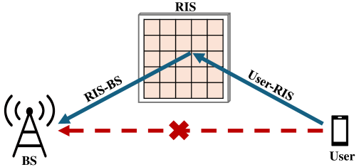
Figure 1: RIS-assisted wireless mmWave communication system.

As illustrated in Fig. 1, we consider a single-input multi-output (SIMO) uplink RIS-assisted mmWave communication system. In this scenario, the direct link between the user and the base station (BS) is blocked, necessitating the deployment of the RIS to facilitate signal transmission. Both the BS and RIS are equipped with uniform planar arrays (UPAs) with elements spaced at half-wavelength intervals. The BS is configured with $M=M_{1}\times M_{2}$ antennas, while the RIS consists of $N=N_{1}\times N_{2}$ passive reflecting elements, where $M_{1}(N_{1})$ and $M_{2}(N_{2})$ are the number of horizontal and vertical antennas, respectively. The UE-RIS channel and the RIS-BS channel are denoted as $\mathbf{h}\in\mathbb{C}^{N\times 1}$ and $\mathbf{G}\in\mathbb{C}^{M\times N}$, respectively. Additionally, we assume that the UE-RIS and the RIS-BS channel remain constant over their respective coherence intervals. Hence, the received signal $\mathbf{y}_{k}\in\mathbb{C}^{M\times 1}$ in $k$-th time slot can be represented as follows

$$\mathbf{y}_{k}=\mathbf{G}diag(\mathbf{\Omega}_{k})\mathbf{h}x_{k}+\mathbf{n},$$ (1)

where the $\mathbf{\Omega}_{k}=[\beta_{1}e^{j\theta_{1}},\beta_{2}e^{j\theta_{2}},\dots,\beta_{M}e^{j\theta_{M}}]^{T}\in\mathbb{C}^{M\times 1}$, $diag(\cdot)$ represents the construction of a diagonal matrix, $\theta\in[-\pi,\pi)$, is the phase shift vector, $\mathbf{n}\sim\mathcal{CN}(0,\sigma^{2}\mathbf{I})\in\mathbb{C}^{M\times 1}$ is additive Gaussian white noise (AWGN), $x_{k}$ is pilot symbol. For $\mathbf{G}$ and $\mathbf{h}$, we adopt geometric channel model[12],

$$\mathbf{G}=\sum_{l=1}^{L_{G}}\sqrt{\frac{MN}{L_{G}}}\alpha_{l}\textbf{a}_{BS}(\theta_{R,l},\phi_{R,l})\textbf{a}_{RIS}^{H}(\theta_{T,l},\phi_{T,l}),$$ (2)

$$\mathbf{h}=\sum_{l=1}^{L_{h}}\sqrt{\frac{N}{L_{h}}}\beta_{l}\textbf{a}_{RIS}(\theta_{R,l},\phi_{R,l}),$$ (3)

where $L_{G}$ and $L_{h}$ are the number of channel paths, $\alpha_{l}$ and $\beta_{l}$ are the complex gain of $l$-th path. $\textbf{a}_{BS}(\theta_{R,l},\phi_{R,l})$ and $\textbf{a}_{RIS}(\theta_{T,l},\phi_{T,l})$ are the steering vectors at BS and RIS, respectively. The $\theta_{R,l}$ and $\phi_{R,l}$ are the azimuth angle and elevation angle of arrival, respectively. Similarly, the $\theta_{T,l}$ and $\phi_{T,l}$ are the azimuth angle and elevation angle of departure, respectively. The interpretation of $\textbf{a}_{RIS}(\theta_{R,l},\phi_{R,l})$ is analogous. The $\textbf{a}_{BS}(\theta_{R,l},\phi_{R,l})$, which is constructed similarly to $\textbf{a}_{RIS}(\theta_{T,l},\phi_{T,l})$ and $\textbf{a}_{RIS}(\theta_{R,l},\phi_{R,l})$, can be written as

$$\textbf{a}_{BS}(\theta_{R,l},\phi_{R,l})=\textbf{a}_{1}(\phi_{R,l})\otimes\textbf{a}_{2}(\theta_{R,l},\phi_{R,l}),$$ (4)

where $\otimes$ denotes Kronecker product. $\textbf{a}_{1}(\phi_{R,l})$ and $\textbf{a}_{2}(\theta_{R,l},\phi_{R,l})$ are given by

$$\textbf{a}_{1}(\phi_{R,l})=\frac{1}{\sqrt{M_{2}}}[ 1,e^{j2\pi\frac{d}{\lambda}cos(\phi_{R,l})},\dots,$$ (5)

$$e^{j2\pi(M_{2}-1)\frac{d}{\lambda}cos(\phi_{R,l})}]^{T},$$

$$\textbf{a}_{2}(\theta_{R,l},\phi_{R,l})=\frac{1}{\sqrt{M_{1}}}[ 1,e^{j2\pi\frac{d}{\lambda}sin(\theta_{R,l})cos(\phi_{R,l})},\dots,$$ (6)

$$e^{j2\pi(M_{1}-1)\frac{d}{\lambda}sin(\theta_{R,l})cos(\phi_{R,l})}]^{T}.$$

Based on (1), the received signals can be rewritten as

$$\mathbf{y}_{k}=\mathbf{G}diag(\mathbf{h})\mathbf{\Omega}_{k}x_{k}+\mathbf{n}.$$ (7)

We define $\mathbf{H}=\mathbf{G}diag(\mathbf{h})$ as the cascaded channel of UE-RIS channel and RIS-BS channel. Without loss of generality, we assume pilot symbol $x_{k}=1$. After $K$ time slots, the received signal $\mathbf{Y}\in\mathbb{C}^{M\times K}$ is

$$\mathbf{Y}=\mathbf{H}\mathbf{\Omega}+\mathbf{N}.$$ (8)

The optimal RIS reflecting matrix is set as the columns of the discrete Fourier transform (DFT) matrix [13]. The objective of channel estimation is to estimate the unknown channel $\mathbf{H}$ from the received signal $\mathbf{Y}$. Given the noise power $\sigma^{2}$, the received signal $\mathbf{Y}$ is normalized as

$$\tilde{\mathbf{Y}}=\frac{1}{\sqrt{1+\sigma^{2}}}\mathbf{Y}=\frac{1}{\sqrt{1+\sigma^{2}}}\mathbf{H}\mathbf{\Omega}+\frac{\sigma}{\sqrt{1+\sigma^{2}}}\mathbf{N}_{0},$$ (9)

where $\mathbf{N}_{0}$ follows the standard Gaussian distribution. We define $\mathbf{X}=\mathbf{H}\mathbf{\Omega}$, so (9) can be rewritten as

$$\tilde{\mathbf{Y}}=\frac{1}{\sqrt{1+\sigma^{2}}}\mathbf{X}+\frac{\sigma}{\sqrt{1+\sigma^{2}}}\mathbf{N}_{0}.$$ (10)

II-B Diffusion Model

Given data distribution $\mathbf{x}_{0}\sim q(\mathbf{x}_{0})$, DM first adds Gaussian noise gradually according to variance schedule $\{\beta_{1},\dots,\beta_{T}\}$. At step $t$, the noised data $\mathbf{x}_{t}$ can be written as

$$\mathbf{x}_{t}=\sqrt{1-\beta_{t}}\mathbf{x}_{t-1}+\beta_{t}\boldsymbol{\epsilon}=\sqrt{\bar{\alpha}_{t}}\mathbf{x}_{0}+\sqrt{1-\bar{\alpha}_{t}}\boldsymbol{\epsilon},$$ (11)

where $\boldsymbol{\epsilon}\sim\mathcal{N}(\mathbf{0},\mathbf{I})$ represents Gaussian noise, $\alpha_{t}=1-\beta_{t}$ and $\bar{\alpha}_{t}=\prod_{s=1}^{t}\alpha_{s}$. The forward diffusion process is formulated as a Markov chain, which is given by

$$q(\mathbf{x}_{t}|\mathbf{x}_{t-1})\sim\mathcal{N}\left(\sqrt{1-\beta_{t}}\mathbf{x}_{t-1},\beta_{t}\mathbf{I}\right).$$ (12)

When $T$ is sufficiently large, the final distribution asymptotically approaches a standard Gaussian distribution. To generate data from $q(\mathbf{x})$, the reverse process is also defined as a parameterized Markov chain [8]

$$p_{\theta}(\mathbf{x}_{t-1}|\mathbf{x}_{t})\sim\mathcal{N}\left(\mathbf{x}_{t-1};\boldsymbol{\mu}_{\theta}(\mathbf{x}_{t},t),\beta_{t}\mathbf{I}\right).$$ (13)

The training process of DM is conducted by optimizing the variational lower bound (VLB) on negative log likelihood [8]

$$\mathbb{E}\left[-\log p_{\theta}(\mathbf{x}_{0})\right]\leq\mathbb{E}_{q}\left[-\log\frac{p_{\theta}(\mathbf{x}_{0:T})}{q(\mathbf{x}_{1:T}|\mathbf{x}_{0})}\right]$$ (14)

$$=\mathbb{E}_{q}\left[-\log p(\mathbf{x}_{T})-\sum_{t\geq 1}\log\frac{p_{\theta}(\mathbf{x}_{t-1}|\mathbf{x}_{t})}{q(\mathbf{x}_{t}|\mathbf{x}_{t-1})}\right]$$

$$=\mathbb{E}_{q}[\underbrace{D_{\text{KL}}(q(\mathbf{x}_{T}|\mathbf{x}_{0})\parallel p(\mathbf{x}_{T}))}_{L_{T}}-\underbrace{\log p_{\theta}(\mathbf{x}_{0}|\mathbf{x}_{1})}_{L_{0}}$$

$$+\sum_{t>1}\underbrace{D_{\text{KL}}(q(\mathbf{x}_{t-1}|\mathbf{x}_{t},\mathbf{x}_{0})\parallel p_{\theta}(\mathbf{x}_{t-1}|\mathbf{x}_{t}))}_{L_{t-1}}],$$

where ${L_{t-1}}$ serves as a denoising matching term and DM realizes the transitions of reverse process by learning the distribution $q(\mathbf{x}_{t-1}|\mathbf{x}_{t},\mathbf{x}_{0})$. According to Bayes rule, $q(\mathbf{x}_{t-1}|\mathbf{x}_{t},\mathbf{x}_{0})$ can be expressed as

$$q(\mathbf{x}_{t-1}|\mathbf{x}_{t},\mathbf{x}_{0})=\frac{q(\mathbf{x}_{t}|\mathbf{x}_{t-1},\mathbf{x}_{0})q(\mathbf{x}_{t-1}|\mathbf{x}_{0})}{q(\mathbf{x}_{t}|\mathbf{x}_{0})}.$$ (15)

Given (9), analytical derivation confirms that $q(\mathbf{x}_{t-1}|\mathbf{x}_{t},\mathbf{x}_{0})$ still follows a Gaussian distribution [8]. Therefore, ${L_{t-1}}$ represents the KL divergence between two Gaussian distributions, which can be calculated in a Rao-Blackwellized fashion with closed form expressions [8].

Based on the analysis of $L_{t-1}$, the mean $\boldsymbol{\mu}_{\theta}(\mathbf{x}_{t},t)$ can be parameterized as follows

$$\boldsymbol{\mu}_{\theta}(\mathbf{x}_{t},t)=\frac{1}{\sqrt{\alpha_{t}}}\left(\mathbf{x}_{t}-\frac{\beta_{t}}{\sqrt{1-\bar{\alpha}_{t}}}\boldsymbol{\epsilon}_{\theta}(\mathbf{x}_{t},t)\right),$$ (16)

where $\boldsymbol{\epsilon}_{\theta}(\mathbf{x}_{t},t)$ represents a neural network parameterized by $\theta$. Given (13) and (16), samples from $\mathbf{x}_{t}$ can be drawn using

$$\mathbf{x}_{t-1}=\frac{1}{\sqrt{\alpha_{t}}}\left(\mathbf{x}_{t}-\frac{1-\alpha_{t}}{\sqrt{1-\bar{\alpha}_{t}}}\boldsymbol{\epsilon}_{\theta}(\mathbf{x}_{t},t)\right)+\sqrt{\beta_{t}}\mathbf{z},$$ (17)

where $\mathbf{z}\sim\mathcal{N}(\mathbf{0},\mathbf{I})$. Accordingly, the loss function of the network $\boldsymbol{\epsilon}_{\theta}(\mathbf{x}_{t},t)$ can be written as

$$L(\theta)=\mathbb{E}_{\mathbf{x}_{0},\epsilon,t}\left[\|\boldsymbol{\epsilon}-\boldsymbol{\epsilon}_{\theta}(\mathbf{x}_{t},t)\|^{2}\right].$$ (18)

III Proposed Method

In this section, we provide a detailed explanation of the proposed method, which leverages the reverse process of DM for channel estimation. First, we reformulate the channel estimation problem within the framework of the reverse diffusion process. Subsequently, to enhance the practical feasibility of DM, we optimize the network architecture, thereby designing a more lightweight and computationally efficient model.

III-A Step Alignment-Based DM-Aided Channel Estimation

Algorithm 1 Training Process

0: Training set $\mathcal{H}$, hyper-parameter $T$ and $\{\beta_{t}\}_{t=1}^{T}$

0: Trained model $\boldsymbol{\epsilon}_{\theta}(\mathbf{x}_{t},t)$

1: repeat

2:  Sample $\mathbf{X}$ from $\mathcal{H}$;

3:  Sample $t$ from $Uniform$({1,…, $T$});

4:  Compute $\mathbf{X}_{t}$ based on (11);

5:  Take gradient descent step according to (18);

6: until converged

Algorithm 2 Sampling Process

0: $\tilde{\mathbf{Y}}$, $t$

0: $\hat{\mathbf{H}}$

1: $\mathbf{X}_{t}=\tilde{\mathbf{Y}}$;

2: for $m=t,\dots,2$ do

3:  Calculate $\mathbf{X}_{m-1}$ based on (20);

4: end for

5: $t=1$;

6: $\mathbf{X}_{0}=\frac{1}{\sqrt{\alpha_{1}}}\left(\mathbf{X}_{1}-\sqrt{1-\bar{\alpha}_{1}}\boldsymbol{\epsilon}_{\theta}(\mathbf{X}_{1},1)\right)$;

7: $\hat{\mathbf{H}}=\mathbf{X}_{0}\mathbf{\Omega}^{\dagger}$;

Due to the presence of channel noise, the accuracy of channel estimation is significantly affected by the noise level. Consequently, mitigating the impact of channel noise is essential for achieving more precise channel estimation. As discussed in Section II, the reverse process of DM inherently serves as a denoising mechanism, which aligns well with our objective of reducing noise-induced errors in channel estimation. Accordingly, we introduce a novel channel estimation framework leveraging DM, wherein an effective denoising strategy is employed to enhance estimation accuracy. In addition, the integration of the step alignment mechanism enables the proposed method to adapt to varying SNR conditions.

Comparing (10) and (11), it can be observed that the received signal is formally similar to the forward process of DM. The received signal can be regarded as the result of progressively adding noise to the noise-free signal, corresponding to a specific step $t$ in the forward process of DM. This inspires us to utilize the reverse process of DM to eliminate channel noise, thereby enhancing the accuracy of channel estimation.

Unlike conventional DM starting with random Gaussian noise [11], the proposed method starts with the normalized received signal $\tilde{\mathbf{Y}}$. The key advantage of starting with $\tilde{\mathbf{Y}}$ is that it enables more accurate channel estimation by incorporating a deterministic received signal to guide the reverse process. However, this also raises the question of how the number of sampling steps should be determined.

In DM, the parameter $\beta_{t}$ denotes the magnitude of noise introduced during the forward process. As the diffusion step progresses, the original signal $\mathbf{x}_{0}$ is increasingly corrupted by noise. Analogously, in communication systems, the received signal experiences noise interference to varying degrees, with the noise power $\sigma^{2}$ serving as a measure of the interference intensity. When $\sqrt{\bar{\alpha}_{t}}=\frac{1}{\sqrt{1+\sigma^{2}}}$, i.e., $\sigma^{2}=\frac{1-\bar{\alpha}_{t}}{\bar{\alpha}_{t}}$, normalized received signal $\tilde{\mathbf{Y}}$ in (10) is aligned with $\mathbf{x}_{t}$ in (11). So the start step can be defined as

$$t=\underset{s}{\text{arg min}}\left|\sigma^{2}-\frac{1-\bar{\alpha}_{s}}{\bar{\alpha}_{s}}\right|.$$ (19)

The initial step varies depending on the noise level, which is reasonable, as a larger step index indicates a higher degree of noise contamination in the signal, thereby necessitating a longer denoising process. By incorporating the step alignment mechanism, the proposed approach is capable of adapting to dynamic noise conditions.

In [8], random noise is introduced during the reverse process, as shown in (17). However, for the channel estimation task, the goal is to obtain a deterministic result, and the inclusion of random noise may interfere with the accuracy of the estimation. Therefore, to improve accuracy, it is crucial to avoid adding random noise during the reverse process [14]. In [9], a deterministic reverse process was proposed, where the predicted noise replaces the random noise. Accordingly, in the reverse process, we adopt the following sampling formula

$$\mathbf{x}_{t-1}=\frac{1}{\sqrt{\alpha_{t}}}\left(\mathbf{x}_{t}-\sqrt{1-\bar{\alpha}_{t}}\boldsymbol{\epsilon}_{\theta}(\mathbf{x}_{t},t)\right)+\sqrt{1-\bar{\alpha}_{t}}\boldsymbol{\epsilon}_{\theta}(\mathbf{x}_{t},t).$$ (20)

In summary, we consider the received signal as the result of the gradual addition of noise to the original signal. Based on (19), we determine the corresponding timestep $t$ and employ a trained neural network $\boldsymbol{\epsilon}_{\theta}(\mathbf{x}_{t},t)$ to iteratively remove the noise from the received signal using the sampling formula (20). Finally, the channel estimation result $\hat{\mathbf{H}}$ is obtained by multiplying the denoising results $\mathbf{X}_{0}$ with the pseudo-inverse of $\mathbf{\Omega}$, denoted as $\mathbf{\Omega}^{\dagger}$. The training process and sampling process are outlined in Algorithm 1 and Algorithm 2, respectively.

III-B Network Architecture Design

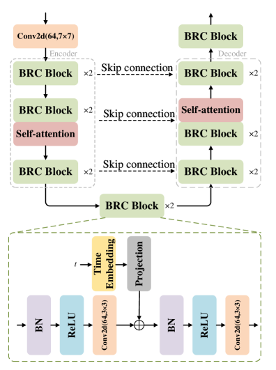
Figure 2: The architecture of the proposed network.

DM typically uses the U-Net, but the large number of parameters and substantial computational loads pose a challenge in resource-limited scenarios. This motivates us to design a lightweight network architecture for practical use. The detailed architecture of the proposed BRCNet is depicted in Fig. 2, the input first passes through a convolutional layer with a kernel size of 7 to expand the receptive field size. Subsequently, an encoder-decoder architecture is employed to capture features at multiple levels. The inclusion of skip connections facilitates the fusion of multi-level feature information by concatenating feature maps from different layers, thereby enhancing the network’s representation capability. Inspired by the DnCNN [15], we designed a low-complexity architecture that employs convolutional layers, batch normalization (BN) layers, and ReLU activation functions as its key components. Furthermore, motivated by the work in [16], we propose a structure in which the activation function is placed before the convolutional layer, forming the Batch normalization–ReLU–Convolutional (BRC) block. This rearrangement further enhances the network’s performance.

Since DM needs to embed the timestep $t$ into the network, we employ sinusoidal embeddings to process the timestep $t$ within the BRC block. After time embedding, a projection module consisting of a Swish activation function and a linear layer projects the embedding vector into an appropriate dimension to facilitate subsequent computations. The detailed structure of the BRC block is illustrated in Fig. 2.

IV Numerical Results

In this section, we conduct simulation experiments to demonstrate the performance of our method. We employ normalized mean square error (NMSE) as the metric of the channel estimation. For channel, we set parameters as follows: $M=M_{1}\times M_{2}=8\times 8$, $N=N_{1}\times N_{2}=4\times 4$, $K=16$, $L_{G}=8$, $L_{h}=1$, $\alpha_{l}\sim\mathcal{CN}(0,1)$, $\beta_{l}\sim\mathcal{CN}(0,1)$. $\theta_{R,l}$, $\phi_{R,l}$, $\theta_{T,l}$ and $\phi_{T,l}$ are uniformly generated from $[-\frac{\pi}{2},\frac{\pi}{2}]$. For DM, the hyper-parameters are set as follows: $T=1000$, the variance schedule $\{\beta_{t}\}$ increases linearly from $\beta_{0}=1\times 10^{-4}$ to $\beta_{T}=0.02$. Dataset is generated using (2)-(6), with the training set consisting of 50,000 samples, while the validation and test sets contain 10,000 samples each. Specifically, the SNR is defined as $\text{SNR}=10\log_{10}\frac{1}{\sigma^{2}}(\text{dB})$.

In the simulations, we consider both the LS method and the LMMSE method for classical channel estimation. Additionally, in [5], the authors employ a deep convolutional network to directly denoise the LS estimation results, denoted as CDRN. In [10], the authors first transform the signal into the angular domain and utilize a lightweight CNN network to achieve channel estimation, denoted as LightCNN. For our proposed method, we implement two different network architectures: U-Net and the proposed BRCNet.

Fig. 3 illustrates the NMSE performance of different methods under varying SNR conditions. It can be observed that the proposed method outperforms all other approaches. Specifically, at SNR = 0 dB, the proposed BRCNet-based method achieves performance gains of 13.50 dB, 11.56 dB, 12.48 dB, and 5.29 dB compared to LS, LMMSE, CDRN, and LightCNN, respectively. Unlike the direct mapping approach used in CDRN, our method improves performance through progressive denoising. Compared to LightCNN, experimental results demonstrate that the proposed network architecture and denoising strategy are more effective in handling the increased complexity of cascaded channels in RIS-assisted systems, thereby achieving superior performance. For the proposed BRCNet, the results indicate that its performance is highly comparable to U-Net, with a performance loss of less than 0.1 dB, while significantly reducing the number of parameters.

As shown in Fig. 4, we investigate the impact of different initial timesteps on channel estimation performance using the proposed BRCNet. The corresponding timesteps $t$ for SNR of $[-10,-5,0,5,10]$ dB are calculated by (19), yielding $[485,373,259,162,93]$, respectively. To analyze the effect of timestep variations, we introduce an offset $\Delta t$ of $[-60,-30,0,30,60]$ and examine the performance changes for different values of $t$. When SNR = $[-5,0,5,10]$ dB, the optimal performance is achieved with timesteps calculated based on (19), validating the correctness of our proposed method. However, at SNR = $-10$ dB, an excessively large timestep degrades performance, suggesting that an upper bound for $t$ should be imposed, as discussed in [9]. Hence, we recommend setting this upper bound as $t_{max}=485$.

In Table I, we compare the number of parameters and the number of inference floating point operations (FLOPs) of different methods. As shown in Table I, BRCNet reduces the number of parameters by approximately 15 times compared to U-Net. Although LightCNN has a significantly smaller parameter count, this reduced capacity limits its performance in complex channel environments. In contrast, BRCNet effectively balances computational complexity and estimation performance. It is worth noting that, compared to methods like CDRN that directly map noisy images to denoised ones, the gradual denoising process of DM can adapt to different SNRs without requiring retraining. This characteristic further reduces the storage requirements and computational burden in practical applications.

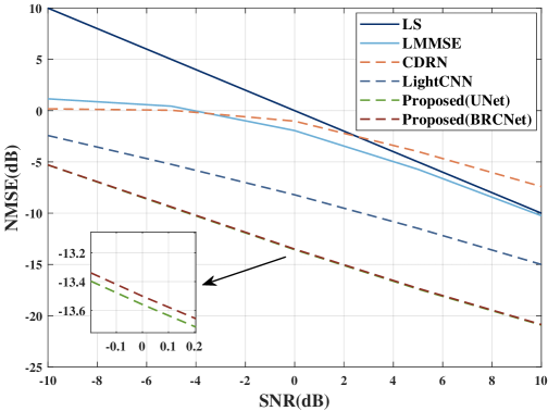
Figure 3: NMSE performance versus SNR.

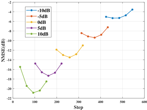
Figure 4: NMSE performance with different start steps using proposed BRCNet.

TABLE I: Complexity and Parameters Comparison

Method	Parameters$\downarrow$	FLOPs$\downarrow$	NMSE$\downarrow$(SNR=0dB)
LightCNN	55.03K	54.0M	-8.21dB
CDRN	1.56M	1.6G	-1.03dB
U-Net	25.81M	6.0G	-13.56dB
Proposed BRCNet	1.70M	1.4G	-13.50dB

• The best and second-best results are highlighted with red and blue backgrounds, respectively.

V Conclusion

In this letter, we propose a DM-aided channel estimation method utilizing the reverse process of DM, which is adaptive to different noise levels. To address network parameter redundancy, we further design a parameter-efficient network that incurs almost no performance loss. Simulation results demonstrate that our method significantly improves performance compared to baselines.

References

- [1] W. Saad, M. Bennis, and M. Chen, “A vision of 6G wireless systems: Applications, trends, technologies, and open research problems,” IEEE Netw., vol. 34, no. 3, pp. 134–142, 2019.
- [2] S. A. Busari, K. M. S. Huq, S. Mumtaz, L. Dai, and J. Rodriguez, “Millimeter-wave massive MIMO communication for future wireless systems: A survey,” IEEE Commun. Surveys Tuts., vol. 20, no. 2, pp. 836–869, 2017.
- [3] Q. Wu and R. Zhang, “Towards smart and reconfigurable environment: Intelligent reflecting surface aided wireless network,” IEEE Commun. Mag., vol. 58, no. 1, pp. 106–112, 2019.
- [4] N. K. Kundu and M. R. McKay, “Channel estimation for reconfigurable intelligent surface aided MISO communications: From LMMSE to deep learning solutions,” IEEE Open J. Commun. Soc., vol. 2, pp. 471–487, 2021.
- [5] C. Liu, X. Liu, D. W. K. Ng, and J. Yuan, “Deep residual learning for channel estimation in intelligent reflecting surface-assisted multi-user communications,” IEEE Trans. Wireless Commun., vol. 21, no. 2, pp. 898–912, 2021.
- [6] Y. Wang, H. Lu, and H. Sun, “Channel estimation in IRS-enhanced mmWave system with super-resolution network,” IEEE Commun. Lett., vol. 25, no. 8, pp. 2599–2603, 2021.
- [7] H. Feng and Y. Zhao, “mmWave RIS-assisted SIMO channel estimation based on global attention residual network,” IEEE Wireless Commun. Lett., vol. 12, no. 7, pp. 1179–1183, 2023.
- [8] J. Ho, A. Jain, and P. Abbeel, “Denoising diffusion probabilistic models,” Advances in neural information processing systems, vol. 33, pp. 6840–6851, 2020.
- [9] T. Wu, Z. Chen, D. He, L. Qian, Y. Xu, M. Tao, and W. Zhang, “CDDM: Channel denoising diffusion models for wireless semantic communications,” IEEE Trans. Wireless Commun., vol. 23, no. 9, pp. 11 168–11 183, 2024.
- [10] B. Fesl, M. B. F. Strasser, M. Joham, and W. Utschick, “Diffusion-based generative prior for low-complexity MIMO channel estimation,” IEEE Wireless Commun. Lett., 2024.
- [11] W. Tong, W. Xu, F. Wang, W. Ni, and J. Zhang, “Diffusion model-based channel estimation for RIS-aided communication systems,” IEEE Wireless Commun. Lett., 2024.
- [12] R. W. Heath, N. González-Prelcic, S. Rangan, W. Roh, and A. M. Sayeed, “An overview of signal processing techniques for millimeter wave MIMO systems,” IEEE J. Sel. Topics Signal Process., vol. 10, no. 3, pp. 436–453, 2016.
- [13] Q.-U.-A. Nadeem, H. Alwazani, A. Kammoun, A. Chaaban, M. Debbah, and M.-S. Alouini, “Intelligent reflecting surface-assisted multi-user MISO communication: Channel estimation and beamforming design,” IEEE Open J. Commun. Soc., vol. 1, pp. 661–680, 2020.
- [14] B. Fesl, B. Böck, F. Strasser, M. Baur, M. Joham, and W. Utschick, “On the asymptotic mean square error optimality of diffusion models,” 2025. [Online]. Available: https://arxiv.org/abs/2403.02957
- [15] K. Zhang, W. Zuo, Y. Chen, D. Meng, and L. Zhang, “Beyond a gaussian denoiser: Residual learning of deep cnn for image denoising,” IEEE Trans. Image Process., vol. 26, no. 7, pp. 3142–3155, 2017.
- [16] K. He, X. Zhang, S. Ren, and J. Sun, “Identity mappings in deep residual networks,” in Computer Vision – ECCV 2016, B. Leibe, J. Matas, N. Sebe, and M. Welling, Eds. Cham: Springer International Publishing, 2016, pp. 630–645.