The stochastic gravitational wave background from QCD phase transition in the framework of higher-order GUP

Abstract

We investigate the stochastic gravitational wave background generated by a first-order cosmological QCD phase transition in the early universe, within the framework of a new higher-order generalized uncertainty principle. This model predicts a minimal length scale for both positive and negative values of the deformation parameter $\beta$. However, our analysis shows that only positive $\beta$ leads to physically viable stochastic gravitational wave background spectra. We derive generalized uncertainty principle induced corrections to the radiation energy density and the Hubble expansion rate and analyze their impact on the resulting stochastic gravitational wave background signal. The results indicate that an increase in $\beta$ leads to a redshift in the peak frequency and a modest enhancement in the energy density. Finally, we examine the detectability of these modified signals by comparing them with the sensitivity curves of current and upcoming pulsar timing arrays. Our findings suggest that the stochastic gravitational wave background signal for positive $\beta$ values can be probed by observatories such as SKA, IPTA, and NANOGrav, offering a potential avenue for testing the effects of quantum gravity effects.

I Introduction

The first direct detection of gravitational waves (GWs) by LIGO in 2015 marked a dual breakthrough in scientific history, it confirmed a prediction of Einstein’s general relativity and inaugurated the field of gravitational wave astronomy, enabling humanity to observe violent cosmic events directly through spacetime vibrations. Subsequent observations by the LIGO and Virgo collaborations uncovered diverse GW sources, including binary black hole mergers [1], neutron star collisions [2], and black hole-neutron star mergers [3]. These groundbreaking discoveries have spurred significant global interest in exploring GWs and their implications for cosmology and fundamental physics.

Nowadays, new generations of gravitational wave detectors are being constructed with heightened sensitivity and extended frequency coverage, targeting gravitational wave signals beyond those emitted by compact binary mergers [4, 5, 6]. Among diverse potential gravitational wave sources, the stochastic gravitational wave background (SGWB) has emerged as an especially compelling and scientifically significant target. The SGWB comprises incoherent superpositions of gravitational waves produced by myriad independent astrophysical and cosmological phenomena, distinguishing it from isolated transient signals associated with compact binary mergers [7, 8, 9]. A dominant cosmological contributor to SGWB arises from phase transitions in the early universe, notably the electroweak phase transition ($T\sim{\rm{100GeV}}$) and the Quantum Chromodynamics (QCD) phase transition ($T\sim{\rm{0.1GeV}}$). When these transitions occur as strongly first-order processes, they efficiently generate gravitational waves through three primary mechanisms: collisions of vacuum bubbles, sound waves propagating in the primordial plasma, and magnetohydrodynamic turbulence [10, 11, 12, 13, 14, 15, 16]. These gravitational waves, originating from disparate spacetime regions and incoherently superposed, collectively form a diffuse, persistent background that encodes fingerprints of high-energy physics inaccessible to terrestrial experiments, thereby offering an unparalleled observational portal to investigate the early universe’s fundamental properties. Crucially, the SGWB is predicted to exhibit characteristic frequencies in $10^{-9}\sim 10^{-6}{\rm{Hz}}$, coinciding with the observational window of Pulsar Timing Arrays (PTAs) including the Square Kilometre Array (SKA) [17], the International Pulsar Timing Array (IPTA) [18], the European Pulsar Timing Array (EPTA) [19], the North American Nanohertz Observatory for Gravitational Waves (NANOGrav) [20], and Chinese Pulsar Timing Array (CPTA) [21]. The operational deployment of these instruments now renders the detection of SGWB increasingly attainable [22]. Collectively, these considerations underscore the imperative to advance theoretical and observational studies of SGWB.

On the other hand, there is growing interest in how quantum gravity (QG) effects might imprint on SGWB [23, 24, 25, 26]. One prominent phenomenological approach to quantum gravity is the generalized uncertainty principle (GUP), which modifies the Heisenberg uncertainty relation to include a minimal length scale (on the order of the Planck length) expected from theories like string theory and loop quantum gravity [27, 28]. The GUP implies that standard commutation relations are deformed at high energies, altering the momentum distribution and thermodynamic properties of particles at extreme densities. In an early universe context, these QG corrections can modify the thermal property, for instance, by altering the blackbody radiation spectrum at high frequencies and introducing deviations from equilibrium thermodynamics [29]. Applying the GUP to cosmological models offers a theoretical pathway to probe potential QG signatures. Specifically, recent studies have investigated how GUP-induced modifications to early-universe thermodynamics could imprint observable features on the SGWB produced by cosmological phase transitions. In Refs. [30, 31, 32], Moussa et al. showed that incorporating two traditional GUP models corrections during a QCD scale first-order phase transition shifts the SGWB spectrum, suppressing the peak frequency of the signal while increasing its amplitude.

Despite their theoretical appeal, the traditional forms of GUP exhibit significant shortcomings [33]. Firstly, foundational models typically involve only low-order corrections, limiting their validity to sub-Planckian momentum regimes and failing to capture physics near the Planck scale. Secondly, standard GUP formulations lack a natural momentum cutoff, unlike quantum gravity frameworks such as doubly special relativity (DSR) that predict a maximal observable momentum. To address these issues, Pedram [34] developed a non-perturbative higher-order GUP framework that aligns with QG principles and resolves conflicts with DSR through a maximal momentum scale. This model marks a critical step toward a consistent QG theory, motivating extensive research into higher-order GUP’s theoretical extensions implications [35, 36, 37, 38, 39]. In parallel, considerable debate has arisen regarding the sign of the GUP parameters in recent years [40]. While a positive GUP parameter has found widespread application in the study of black hole characteristics, it also introduces challenges in other contexts. For instance, in the study of compact objects, a positive parameter can lead to the breakdown of the Chandrasekhar limit, casting doubt on the viability of white dwarfs and neutron stars [41]. Interestingly, adopting a negative GUP parameter resolves this inconsistency, restoring the limiting mass and offering a more coherent description of gravitational equilibrium [42]. In addition, it is found that the negative GUP parameters may arise in non-trivial spacetime structures and result in a crystalline-like universe [43, 44]. Those divergence in physical predictions have prompted renewed interest in the sign dependence of GUP models and in exploring the broader implications of higher-order and sign-reversed formulations within different QG scenarios.

Recently, Du and Long [45] has proposed a new higher-order GUP model, which can be expressed as:

$$\Delta x\Delta p\geq\frac{\hbar}{2}\frac{1}{{1\pm\left({{{16\beta}\mathord{\left/{\vphantom{{16\beta}{\Delta{x^{2}}}}}\right.\kern-1.2pt}{\Delta{x^{2}}}}}\right)}},$$ (1)

where $\Delta p$ and $\Delta x$ are the uncertainties for momentum and position, respectively. $\beta={{\beta_{0}}\ell_{p}^{2}}$ with the GUP parameter $\beta_{0}$. This model addresses the inconsistency of the minimum length under varying parameter signs, offering several distinctive features. First, it introduces parameter adaptability, where the GUP parameter can be either positive or negative, yet the minimum length remains unified as $\Delta{x_{\min}}=4\sqrt{|{\beta_{0}}|}{\ell_{p}}$, independent of the sign of GUP parameter. Second, the modified structure replaces the traditional momentum-squared term with a position-squared correction, ensuring consistency even for negative $\beta$. Third, a maximum momentum $\Delta{p_{\max}}={\hbar\mathord{\left/{\vphantom{\hbar{\left({16\sqrt{|\beta|}{\ell_{p}}}\right)}}}\right.\kern-1.2pt}{\left({16\sqrt{|\beta|}{\ell_{p}}}\right)}}$ naturally emerges for $\beta>0$ aligning with higher-order GUP predictions. Lastly, the unified minimum length is model-independent, reinforcing its universality in quantum gravity frameworks. These advancements resolve contradictions in existing GUP formulations while preserving compatibility with diverse QG scenarios. Subsequently, researchers explored the cosmological dynamics and thermodynamic properties under both positive and negative GUP parameters based on this model, uncovering novel features of cosmic phase transitions and their impact on nucleosynthesis in the universe. These findings demonstrate that the new GUP framework can significantly influence cosmological properties [46, 47, 48]. This naturally raises the question: Can this GUP model be reconciled with the theory of SGWB? What are the distinguishing features of SGWB under positive versus negative GUP parameters? To address these questions, we attempt in this manuscript to derive a modified SGWB spectrum using GUP (1), analyzing its characteristic frequencies and fractional energy density. Finally, we discuss the implications of QG effects on the SGWB signature.

The structure of this paper is as follows. In the section II, we derive the general expression for the SGWB spectrum observed today within the framework of the new higher-order GUP (1). Section III presents the construction of the effective equation of state employed in this work, obtained by comparing the ideal gas phase with the QCD equation of state from recent lattice simulations. In Section V, we investigate the influence of the higher-order GUP on the amplitude and frequency characteristics of the SGWB, and explore the potential signatures detectable by current and future gravitational wave observatories. Finally, Section VI summarizes the main findings and provides concluding remarks.

II Higher-order GUP corrected entropy and photons gas

In the framework of new higher-order GUP (1), the canonical commutation relation between position and momentum operators is modified to include a position-dependent correction of the form

$$\left[{{x_{i}},{p_{j}}}\right]=i\hbar\frac{1}{{1\pm\left({{{16\beta}\mathord{\left/{\vphantom{{16\beta}{{x^{2}}}}}\right.\kern-1.2pt}{{x^{2}}}}}\right)}}{\delta_{ij}}.$$ (2)

where $x$ is the characteristic length scale of the system. The uncertainty relation (2) implies the existence of a minimal measurable length or a maximal observable momentum, depending on the sign and magnitude of $\beta$. Such a deformation can be realized through a symmetric operator representation

$${p_{i}}=\frac{1}{{1\pm\left({{{16\beta}\mathord{\left/{\vphantom{{16\beta}{{x^{2}}}}}\right.\kern-1.2pt}{{x^{2}}}}}\right)}}{p_{0i}},\quad{x_{i}}={x_{0i}},$$ (3)

where $p_{0i}$ and $x_{0i}$ satisfy the usual Heisenberg algebra $\left[{{x_{i0}},{p_{j0}}}\right]=i\hbar{\delta_{ij}}$.

As a consequence of the modified commutation relation (3), the canonical volume element in phase space is no longer invariant. According to Liouville’s theorem, the number of quantum states in phase space must remain fixed under time evolution. Therefore, the nontrivial Jacobian of the momentum transformation must be taken into account, leading to a deformation in the number of quantum states per momentum space volume as

$$\frac{V}{{{{\left({2\pi}\right)}^{3}}}}\int_{0}^{\infty}{{{\rm{d}}^{3}}p}\to\frac{V}{{{{\left({2\pi}\right)}^{3}}}}\int_{0}^{\infty}{{{\left({1\pm 16\beta{x^{-2}}}\right)}^{3}}{{\rm{d}}^{3}}p}.$$ (4)

In order to investigate the thermodynamic consequences of the modified phase space measure, we consider a gas of massless bosons, specifically photons. This choice is motivated by the fact that, in the early universe, radiation dominated the energy content, and photons constituted a significant portion of the thermal plasma. Furthermore, due to their vanishing mass and bosonic nature, photons obey the Bose-Einstein distribution and provide an analytically tractable system for computing the partition function and entropy. These thermodynamic quantities, once modified by GUP, will play a crucial role in determining the redshift of the stochastic gravitational wave background generated during the QCD phase transition. To proceed, we consider the thermal correspondence $\Delta x\sim{T^{-1}}$, which is appropriate for the radiation-dominated epoch of the early universe. This allows us to reexpress the position-dependent GUP correction in terms of temperature. Consequently, the modified number of quantum states per unit momentum space volume becomes:

$$\frac{V}{{{{\left({2\pi}\right)}^{3}}}}\int_{0}^{\infty}{{{\rm{d}}^{3}}p}\to\frac{V}{{{{\left({2\pi}\right)}^{3}}}}\int_{0}^{\infty}{{{\left({1\pm 16\beta{T^{2}}}\right)}^{3}}{{\rm{d}}^{3}}p}.$$ (5)

According to Eq. (5), the modified partition function per unite volume is

$$\ln Z =-\frac{{{g_{\pi}}}}{{2{\pi^{2}}}}\int_{0}^{\infty}{\ln\left[{1-\exp\left({-\frac{p}{T}}\right)}\right]}\left({1\pm 16\beta{T^{2}}}\right){p^{2}}{\rm{d}}p$$

$$=\frac{{{g_{\pi}}{\pi^{2}}}}{{90}}{T^{3}}{\left({1\pm 16\beta{T^{2}}}\right)^{3}},$$ (6)

where ${g_{\pi}}$ is to the number of degrees of freedom. This partition function forms the basis for computing thermodynamic quantities. From the deformed phase space and statistical distribution, the modified entropy of photon gas is given by

$$S_{{\rm{GUP}}} =\frac{\partial}{{\partial T}}\left({T\ln Z}\right)$$

$$=\frac{2}{{45}}{\pi^{2}}{g_{\pi}}{T^{3}}\left({1\pm 72\beta{T^{2}}+1536\beta^{2}{T^{4}}\pm 10240\beta^{3}{T^{6}}}\right).$$ (7)

When ignoring the quantum gravity effects (i.e., $\beta\to 0$), the modified entropy reduces smoothly to the standard expression ${S_{0}}={{2{\pi^{2}}{g_{\pi}}{T^{3}}}\mathord{\left/{\vphantom{{2{\pi^{2}}{g_{\pi}}{T^{3}}}{45}}}\right.\kern-1.2pt}{45}}$ [49]. Utilizing these derived results of the modified entropy and partition function, in the next section, we will systematically investigate how the higher-order GUP corrections influence the evolution of the stochastic gravitational wave background generated during the cosmological QCD phase transition.

III Impact of higher-order GUP modified entropy on the SGWB spectrum

In investigating the influence of the GUP on the generation and evolution of the SGWB, a foundational task is to establish the thermodynamic structure of the universe that is consistent with the GUP correction. However, the introduction of a minimal measurable length or maximal momentum, as predicted by GUP, modifies the phase space volume (e.g., Eq. (4)), which in turn affects the statistical mechanics of radiation fields. In the framework of standard cosmology, the photon-dominated entropy density of the radiation field $\mathbb{S}\sim{a^{3}}{S_{0}}\sim{a^{3}}\left({{{2{\pi^{2}}{g_{s}}{T^{3}}}\mathord{\left/{\vphantom{{2{\pi^{2}}{g_{s}}{T^{3}}}{45}}}\right.\kern-1.2pt}{45}}}\right)$ with the scale factor $a$ and the effective number of degrees of freedom $g_{s}$, plays a crucial role in determining the dynamics of the cosmic expansion, whereas in the framework of the GUP, due to the introduction of the minimum length or the maximum momentum, the density of the quantum states as well as the collocation function are corrected, which leads to the systematic change of the statistical mechanical quantities. While Refs. [30, 31, 32] have proposed GUP corrected entropy expressions by modifying the density of states, these studies often retain only leading-order corrections (e.g., linear or quadratic in temperature). Such truncations are reasonable at low temperatures, but they become insufficient near high energy scales, especially around the QCD phase transition, where higher-order QG effects can no longer be neglected.

Now, applying the GUP corrected entropy (II), the relevant entropy density can be expressed as

$${\mathbb{S}_{{\rm{GUP}}}}={a^{3}}{g_{s}}\frac{2}{{45}}{\pi^{2}}{T^{3}}\left({1\pm 72\beta{T^{2}}+1536\beta^{2}{T^{4}}\pm 10240\beta^{3}{T^{6}}}\right).$$ (8)

Then, according to the adiabatic condition ${{\dot{\mathbb{S}}}\mathord{\left/{\vphantom{{\dot{\mathbb{S}}}{\mathbb{S}}}}\right.\kern-1.2pt}{\mathbb{S}}}=0$, which implies that the total entropy remains conserved during the expansion of the universe, the time variation of the universe temperature in the presence of GUP corrections as

$$\frac{{{\rm{d}}T}}{{{\rm{d}}t}}=-HT{\Delta}{\left({T,g_{s},\beta}\right)^{-1}},$$ (9)

with

$${\Delta}\left({T,g_{s},\beta}\right)=1+\frac{T}{{3{g_{s}}}}\frac{{{\rm{d}}{g_{s}}}}{{{\rm{d}}T}}+\frac{{16\beta{T^{2}}\left({80\beta{T^{2}}\pm 3}\right)}}{{1\pm 56\beta{T^{2}}+640{\beta^{2}}{T^{4}}}}.$$ (10)

For $\beta_{0}=0$, the original case $\Delta=1+\left({{T\mathord{\left/{\vphantom{T{3{g_{s}}}}}\right.\kern-1.2pt}{3{g_{s}}}}}\right)\left({{{{\rm{d}}{g_{s}}}\mathord{\left/{\vphantom{{{\rm{d}}{g_{s}}}{{\rm{d}}T}}}\right.\kern-1.2pt}{{\rm{d}}T}}}\right)$ is recovered. Due to the Hubble parameter, one has

$$\frac{{{a_{*}}}}{{{a_{0}}}}=\exp\left({\int_{{T_{*}}}^{{T_{0}}}{{T^{-1}}\Delta{\rm{d}}T}}\right),$$ (11)

where the indices “*” and “0” denote the corresponding physical parameters evaluated at the time of the phase transition and the present era, respectively. Using the relationship between the scale factor and redshift ${{{\nu_{0{\rm{peak}}}}}\mathord{\left/{\vphantom{{{\nu_{0{\rm{peak}}}}}{{\nu_{*}}}}}\right.\kern-1.2pt}{{\nu_{*}}}}={{{a_{*}}}\mathord{\left/{\vphantom{{{a_{*}}}{{a_{0}}}}}\right.\kern-1.2pt}{{a_{0}}}}$, the redshift corresponding to the peak frequency of SGWB relative to its present value can be formulated as follows

$$\frac{{{\nu_{0{\rm{peak}}}}}}{{{\nu_{*}}}}=\frac{{{a_{*}}}}{{{a_{0}}}}=\frac{{{T_{0}}}}{{{T_{*}}}}{\left[{\frac{{{g_{s}}\left({{T_{0}}}\right)}}{{{g_{s}}\left({{T_{*}}}\right)}}}\right]^{\frac{1}{3}}}{\left({\frac{{1\pm 16\beta T_{0}^{2}}}{{1\pm 16\beta T_{*}^{2}}}}\right)^{\frac{2}{3}}}{\left({\frac{{1\pm 40\beta T_{0}^{2}}}{{1\pm 40\beta T_{*}^{2}}}}\right)^{\frac{1}{3}}}.$$ (12)

To examine the role of the GUP effect in modifying the ratio of the peak frequency of the present SGWB to the frequency at the QCD phase transition epoch, we illustrate this relationship in Fig. 1.

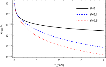
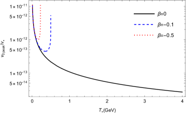
Figure 1: ${{{\nu_{0{\rm{peak}}}}}\mathord{\left/{\vphantom{{{\nu_{0{\rm{peak}}}}}{{\nu_{*}}}}}\right.\kern-1.2pt}{{\nu_{*}}}}$ for different values of GUP parameters, we set ${T_{0}}=2.725K=2.348\times{10^{-13}}{\text{GeV}}$, $g_{s}\left({{T_{0}}}\right)=3.4$ and $g_{s}\left({{T_{*}}}\right)=35$. (a) Positive GUP parameters. (b) Negative GUP parameters.

Fig. 1 shows how the ratio of the peak frequency of the present SGWB to the frequency at the QCD phase transition epoch ${{{\nu_{0{\rm{peak}}}}}\mathord{\left/{\vphantom{{{\nu_{0{\rm{peak}}}}}{{\nu_{*}}}}}\right.\kern-1.2pt}{{\nu_{*}}}}$ varies with the QCD phase transition temperature $T_{*}$ under different values of the higher-order GUP parameter $\beta$. Fig. 1 illustrates the case for positive GUP parameters. Without the effects of GUP ($\beta=0$), the frequency ratio demonstrates a stable decreasing trend. With increasing positive $\beta$ values, the frequency ratio decreases significantly, indicating a strong suppression effect of positive GUP parameters on the current SGWB peak frequency. This suppression effect becomes more pronounced as the transition temperature increases. Fig. 1 presents the scenario with negative GUP parameters, revealing a distinctly opposite behavior. As the absolute value of negative $\beta$ increases, the frequency ratio increases rapidly with increasing transition temperature and exhibits a divergence at certain high temperatures. This divergence suggests limitations or internal inconsistencies of the negative GUP parameter model at high temperatures approaching the Planck scale, implying that the negative GUP effect may exceed the self-consistent theoretical framework under extreme early universe conditions. Thus, in the following study, the case of negative parameters will no longer be discussed.

We now turn to the evolution of the SGWB energy density. Since GWs decouple from the thermal plasma shortly after their generation, their energy density satisfies the Boltzmann equation ${{{\rm{d}}\left({{\rho_{{\rm{gw}}}}{a^{4}}}\right)}\mathord{\left/{\vphantom{{{\rm{d}}\left({{\rho_{{\rm{gw}}}}{a^{4}}}\right)}{{\rm{d}}t}}}\right.\kern-1.2pt}{{\rm{d}}t}}=0$. This relation enables us to track the redshift behavior of the SGWB energy density from the phase transition epoch to the present era. The energy density of the SGWB at the present time is given by

$${\rho_{{\rm{gw}}}}\left({{T_{0}}}\right)={\rho_{{\rm{gw}}}}\left({{T_{*}}}\right){\left({\frac{{{a_{*}}}}{{{a_{0}}}}}\right)^{4}}={\rho_{{\rm{gw}}}}\left({{T_{*}}}\right)\exp\left({\int_{{T_{*}}}^{{T_{0}}}{4{T^{-1}}}\Delta{\rm{d}}T}\right).$$ (13)

Next, based on Eq. (13) and the definitions of the SGWB energy density parameters at the phase transition temperature $T_{*}$ and the present temperature $T_{0}$, given by ${\Omega_{{\rm{gw_{*}}}}}={{{\rho_{{\rm{gw}}}}\left({{T_{*}}}\right)}\mathord{\left/{\vphantom{{{\rho_{{\rm{gw}}}}\left({{T_{*}}}\right)}{{\rho_{cr}}\left({{T_{*}}}\right)}}}\right.\kern-1.2pt}{{\rho_{cr}}\left({{T_{*}}}\right)}}$ and ${\Omega_{{\rm{gw}}}}={{{\rho_{{\rm{gw}}}}\left({{T_{0}}}\right)}\mathord{\left/{\vphantom{{{\rho_{{\rm{gw}}}}\left({{T_{0}}}\right)}{{\rho_{\rm{cr}}}\left({{T_{0}}}\right)}}}\right.\kern-1.2pt}{{\rho_{\rm{cr}}}\left({{T_{0}}}\right)}}$, the expression for the SGWB energy density at parameter present time reads

$${\Omega_{{\rm{gw}}}}={\Omega_{{\rm{gw_{*}}}}}{\left({\frac{{{H_{*}}}}{{{H_{0}}}}}\right)^{2}}\exp\left({\int_{{T_{*}}}^{{T_{0}}}{4{T^{-1}}}\Delta{\rm{d}}T}\right)$$ (14)

where

$${\left({\frac{{{H_{*}}}}{{{H_{0}}}}}\right)^{2}}=\frac{{{\rho_{{\rm{cr}}}}\left({{T_{*}}}\right)}}{{{\rho_{{\rm{cr}}}}\left({{T_{0}}}\right)}}.$$ (15)

For the purpose of gaining the ratio of Hubble parameter during the cosmic phase transition to its present-day value, we are supposed to leverage the continuity equation $\dot{\rho}_{t}=-3H\rho_{t}\left(1+\frac{P_{t}}{\rho_{t}}\right)$, where $P_{t}$ represents the total pressure density of the universe and $\rho_{t}$ is the total energy density of the universe, respectively. By expressing the continuity equation in terms of temperature and substituting Eq. (9), one gets

$$\frac{{{\rm{d}}{\rho_{t}}}}{{{\rho_{t}}}}=\frac{3}{T}\left({1+{\omega_{{\rm{eff}}}}}\right)\Delta{\rm{d}}T,$$ (16)

with the effective equation of state (EOS) parameter ${{\omega_{{\rm{eff}}}}={{{P_{t}}}\mathord{\left/{\vphantom{{{P_{t}}}{{\rho_{t}}}}}\right.\kern-1.2pt}{{\rho_{t}}}}}$. By integrating Eq. (9) from the early radiation-dominated era (characterized by a temperature $T_{r}=10^{4}\mathrm{GeV}$) to the phase transition temperature $T_{*}$, the critical energy density of radiation during the phase transition is given by

$${\rho_{{\rm{cr}}}}\left({{T_{*}}}\right)={\rho_{r}}\left({{T_{r}}}\right)\exp\left[{\int_{{T_{r}}}^{{T_{*}}}{\frac{3}{T}}\left({1+{\omega_{{\rm{eff}}}}}\right)\Delta{\rm{d}}T}\right].$$ (17)

Then, by substituting $\rho_{\rm{cr}}(T_{*})$ from Eq. (17) into Eq. (15), one obtains

$${\left({\frac{{{H_{*}}}}{{{H_{0}}}}}\right)^{2}}={\Omega_{r0}}\frac{{{\rho_{r}}\left({{T_{r}}}\right)}}{{{\rho_{r}}\left({{T_{0}}}\right)}}\exp\left[{\int_{{T_{r}}}^{{T_{*}}}{\frac{3}{T}}\left({1+{\omega_{{\rm{eff}}}}}\right)\Delta{\rm{d}}T}\right],$$ (18)

where the current fractional energy density of radiation is $\Omega_{r0}=\rho_{r}\left(T_{0}\right)/\rho_{cr}\left(T_{0}\right)\simeq 8.5\times 10^{-5}$. Moreover, by applying the Boltzmann equation, it is found that $\rho_{r}(T_{r})/\rho_{r}(T_{0})\simeq(a_{0}/a_{r})^{4}$ [32]. Therefore, Eq. (18) can be rewritten as

$${\left({\frac{{{H_{*}}}}{{{H_{0}}}}}\right)^{2}}={\Omega_{r0}}\exp\left({\int_{{T_{0}}}^{{T_{r}}}{\frac{4}{T}}\Delta{\rm{d}}T}\right)\exp\left[{\int_{{T_{r}}}^{{T_{*}}}{\frac{3}{T}}\left({1+{\omega_{{\rm{eff}}}}}\right)\Delta{\rm{d}}T}\right].$$ (19)

Finally, by using Eq. (19) and Eq. (14), the GWs spectrum observed today can be expressed as

$${\Omega_{{\rm{gw}}}}={\Omega_{r0}}{\Omega_{{\rm{g}}{{\rm{w}}_{*}}}}\exp\left({\int_{{T_{*}}}^{{T_{r}}}{\frac{4}{T}}\Delta{\rm{d}}T}\right)\exp\left[{\int_{{T_{r}}}^{{T_{*}}}{\frac{3}{T}}\left({1+{\omega_{{\rm{eff}}}}}\right)\Delta{\rm{d}}T}\right].$$ (20)

The above equation describes the present-day energy density spectrum of GWs, linking the initial spectrum at the phase transition epoch $\Omega_{{\rm gw}_{*}}$ to its observable form today. The factor $\Omega_{r0}$ accounts for the current radiation energy density, while the exponential terms encode the impact of the universe’s expansion history. More importantly, the integrands contain the function ${\Delta}\left({T,g_{s},\beta}\right)$, which incorporates modifications arising from the effect of GUP. The GUP-induced corrections modify the standard thermodynamic relations, thereby influencing the evolution of the Hubble parameter and the redshift of GWs.

IV Influence of non-ideal equation of state on SGWB during the QCD phase transition

In this section, we examine the impact of the effective EOS on the spectral characteristics of the SGWB, with particular attention to the role of non-ideal QCD interactions and trace anomaly effects. These factors become especially significant during the QCD phase transition, where strong interactions among quarks and gluons induce substantial deviations from the ideal relativistic gas approximation commonly used in cosmological models. In addition, we investigate how higher-order GUP corrections further influence the EOS and SGWB evolution, highlighting the relevance of QG effects in this cosmological epoch.

For an ultra-relativistic ideal gas composed of non-interacting particles, the effective EOS parameter is given by ${{\omega_{{\rm{eff}}}}={1\mathord{\left/{\vphantom{13}}\right.\kern-1.2pt}3}}$ [50]. Under this condition, Eq. (19) and Eq. (20) can be recast into the following analytical expressions:

$${\left({\frac{{{H_{*}}}}{{{H_{0}}}}}\right)^{2}}={\Omega_{r0}}{\left({\frac{{{T_{*}}}}{{{T_{0}}}}}\right)^{4}}{\left[{\frac{{{g_{s}}\left({{T_{*}}}\right)}}{{{g_{s}}\left({{T_{0}}}\right)}}}\right]^{\frac{4}{3}}}{\left({\frac{{1+16\beta T_{0}^{2}}}{{1+16\beta T_{*}^{2}}}}\right)^{\frac{8}{3}}}{\left({\frac{{1+40\beta T_{0}^{2}}}{{1+40\beta T_{*}^{2}}}}\right)^{\frac{2}{3}}},$$ (21)

$${\Omega_{{\rm{gw}}}}={\Omega_{r0}}{\Omega_{{\rm{gw}}}},$$ (22)

Notably, the present-day SGWB spectrum described by Eq. (22) reverts to its standard form, indicating that the GUP parameter $\beta$ ceases to influence the observed spectral features. However, this idealized scenario diverges from reality when QCD interactions are incorporated, as they induce deviations from $\omega_{\rm{eff}}=1/3$. These deviations can substantially modify the SGWB spectrum relative to the non-interacting case, highlighting the importance of incorporating a refined EOS during the QCD epoch [51].

To incorporate the effects of QCD interactions, we employ results from modern lattice QCD calculations using $N_{f}=2+1$ flavors, which reliably cover the temperature range from $0.1~\rm{GeV}$ to $0.4~\rm{GeV}$. These calculations enable a realistic description of the strongly interacting plasma. Accordingly, the EOS of QCD is constructed based on the parameterization of the pressure, reflecting the contributions from the strong interactions among $u$, $d$ and $s$ quarks and gluons. The parameterized expression for the QCD pressure reads

$$F\left(T\right)=\frac{P}{{{T^{4}}}}=\frac{{1+\tanh\left[{{c_{\tau}}\left({\tau-{\tau_{0}}}\right)}\right]}}{2}\frac{{{p_{i}}+\frac{{{a_{n}}}}{\tau}+\frac{{{b_{n}}}}{{{\tau^{2}}}}+\frac{{{c_{n}}}}{{{\tau^{4}}}}}}{{1+\frac{{{a_{d}}}}{\tau}+\frac{{{b_{d}}}}{{{\tau^{2}}}}+\frac{{{c_{d}}}}{{{\tau^{4}}}}}}.$$ (23)

Here, the dimensionless temperature ratio is defined as $\tau={T\mathord{\left/{\vphantom{T{{T_{c}}}}}\right.\kern-1.2pt}{{T_{c}}}}$, with the critical temperature taken as $T_{c}=0.145~\rm{GeV}$, corresponding to the QCD phase transition. For a system of three massless quark flavors, the ideal gas limit of the normalized pressure is given by ${p_{i}}={{19{\pi^{2}}}\mathord{\left/{\vphantom{{19{\pi^{2}}}{36}}}\right.\kern-1.2pt}{36}}$. At temperatures above $100~\rm{MeV}$, and the fitting parameters are specified as follows:

$$a_{n}=-8.7704,\quad b_{n}=3.9200,\quad c_{n}=0.3419,\quad a_{d}=-1.2600,\quad b_{d}=0.8425,\quad c_{d}=-0.0475.$$ (24)

Notably, during the QCD phase transition, the EOS deviates from the ideal behavior due to strong interactions, and pressure alone becomes insufficient to fully characterize the thermodynamic properties of the system. To address this, we invoke the trace anomaly relation [52], which connects the pressure and energy density through the breaking of conformal symmetry in QCD:

$$\frac{\rho-3P}{T^{4}}=T\frac{\mathrm{d}F(T)}{\mathrm{d}T}=T\frac{\mathrm{d}}{\mathrm{d}T}\left(\frac{P}{T^{4}}\right),$$ (25)

Accordingly, when effects of QCD are taken into account, the effective EOS parameter incorporating the trace anomaly can be expressed as

$$\omega_{\mathrm{eff}}=\left[\frac{T}{F\left(T\right)}\frac{\mathrm{d}F\left(T\right)}{\mathrm{d}T}+3\right]^{-1}.$$ (26)

Based on Eq. (26), the relationship between the effective EOS $\omega_{\rm{eff}}$ and the transition temperature $T_{*}$ is illustrated in Fig. 2. It can be seen that, at high temperatures ($T_{*}\geq 5~\rm{GeV}$) asymptotically approaches the ideal gas limit of ${1\mathord{\left/{\vphantom{13}}\right.\kern-1.2pt}3}$, indicating negligible interaction effects. However, in the lower temperature range (${T_{*}}\sim 0.1-0.3~\rm{GeV}$), which corresponds to the QCD phase transition epoch, $\omega_{\rm{eff}}$ deviates significantly from the ideal value due to the strong interactions among quarks and gluons. This deviation highlights the necessity of incorporating realistic QCD effects into the SGWB analysis.

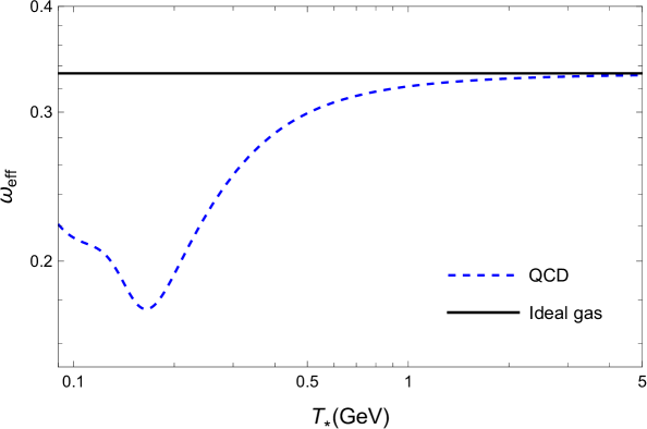
Figure 2: The relationship between the effective EOS $\omega_{\rm{eff}}$ and transition temperature $T_{*}$.

Then, by substituting the effective EOS parameter incorporating the trace anomaly (26) into Eq. (20), the Hubble parameter ratio between the transition epoch and the present epoch can be expressed as

$${\left({\frac{{{H_{*}}}}{{{H_{0}}}}}\right)^{2}} ={\Omega_{r0}}{\left({\frac{{{T_{r}}}}{{{T_{0}}}}}\right)^{4}}{\left[{\frac{{{g_{s}}\left({{T_{r}}}\right)}}{{{g_{s}}\left({{T_{0}}}\right)}}}\right]^{\frac{4}{3}}}{\left({\frac{{1+16\beta T_{r}^{2}}}{{1+16\beta T_{0}^{2}}}}\right)^{\frac{8}{3}}}{\left({\frac{{1+40\beta T_{r}^{2}}}{{1+40\beta T_{0}^{2}}}}\right)^{\frac{2}{3}}}$$

$$\times\frac{{{g_{s}}{{\left({{T_{*}}}\right)}^{1+\omega\left({{T_{*}}}\right)}}}}{{{g_{s}}{{\left({{T_{r}}}\right)}^{1+\omega\left({{T_{r}}}\right)}}}}\exp\left\{{\int_{{T_{r}}}^{{T_{*}}}{\frac{{3\left({1+\omega}\right)}}{T}\left[{1+\frac{{16\beta{T^{2}}\left({3+80\beta{T^{2}}}\right)}}{{1+56\beta{T^{2}}+640{\beta^{2}}{T^{4}}}}}\right]{\rm{d}}T}}\right\},$$ (27)

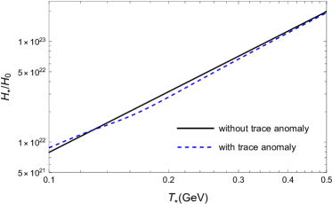
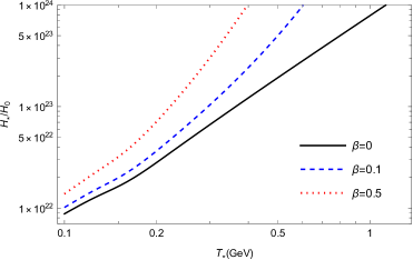
Figure 3: The relationship between the ${{{H_{*}}}\mathord{\left/{\vphantom{{{H_{*}}}{{H_{0}}}}}\right.\kern-1.2pt}{{H_{0}}}}$ and transition temperature $T_{*}$. We set $T_{r}=10^{4}~\rm{GeV}$. (a) Without the effect of GUP. (b) With different values of GUP parameter.

From Fig. 3, one can see the variation of the Hubble parameter ratio ${{{{H_{*}}}\mathord{\left/{\vphantom{{{H_{*}}}{{H_{0}}}}}\right.\kern-1.2pt}{{H_{0}}}}}$ as a function of the QCD phase transition temperature $T_{*}$ under different conditions according to Eq. (IV). Fig. 3 compares the scenarios with (blue dashed curve) and without (black solid curve) the inclusion of the QCD trace anomaly effect. In the lower temperature range (${T_{*}}\sim 0.1-0.15~\rm{GeV}$), the blue dashed curve is notably above the black solid curve, indicating that the trace anomaly significantly enhances the Hubble parameter ratio. However, as the transition temperature increases to the intermediate range (${T_{*}}\sim 0.15-0.5~\rm{GeV}$) , the trend reverses, and the black solid line exceeds the blue dashed line, indicating a reduced impact of the trace anomaly effect compared to the ideal gas case. When the temperature is higher than $0.5~\rm{GeV}$, the two curves gradually converge, showing that QCD interactions become negligible, and both cases approach the ideal relativistic gas limit. These results highlight the temperature-dependent significance of the trace anomaly and the necessity for accurate QCD thermodynamics when analyzing the cosmological evolution of the SGWB. Fig. 3 demonstrates the influence of positive GUP parameters $\beta=0.1$ and $\beta=0.5$, where increasing $\beta$ leads to a notable enhancement in the Hubble parameter ratio, especially at higher transition temperatures. These results highlight the combined effects of QCD thermodynamics and QG corrections on the expansion history of the early universe.

Then, incorporating the influence of the trace anomaly alongside Eq. (20), the of GW energy density parameter ratio is given by

$$\frac{{{\Omega_{{\rm{gw}}}}}}{{{\Omega_{{\rm{gw*}}}}}}={\Omega_{r0}}{\left({\frac{{{T_{r}}}}{{{T_{*}}}}}\right)^{4}}{\left({\frac{{{g_{s}}\left({{T_{r}}}\right)}}{{{g_{s}}\left({{T_{*}}}\right)}}}\right)^{\frac{4}{3}}}{\left({\frac{{1+16\beta T_{r}^{2}}}{{1+16\beta T_{*}^{2}}}}\right)^{\frac{8}{3}}}{\left({\frac{{1+40\beta T_{r}^{2}}}{{1+40\beta T_{*}^{2}}}}\right)^{\frac{2}{3}}}$$

$$\times\frac{{{g_{s}}{{\left({{T_{*}}}\right)}^{1+\omega\left({{T_{*}}}\right)}}}}{{{g_{s}}{{\left({{T_{r}}}\right)}^{1+\omega\left({{T_{r}}}\right)}}}}\exp\left\{{\int_{{T_{r}}}^{{T_{*}}}{\frac{{3\left({1+\omega}\right)}}{T}\left[{1+\frac{{16\beta{T^{2}}\left({3+80\beta{T^{2}}}\right)}}{{1+56\beta{T^{2}}+640{\beta^{2}}{T^{4}}}}}\right]{\rm{d}}T}}\right\}.$$ (28)

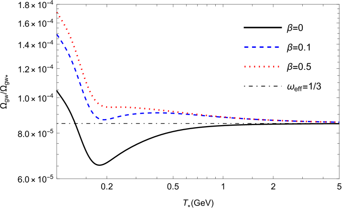
Figure 4: The relationship between ${{{\Omega_{{\rm{gw}}}}}\mathord{\left/{\vphantom{{{\Omega_{{\rm{gw}}}}}{{\Omega_{{\rm{gw*}}}}}}}\right.\kern-1.2pt}{{\Omega_{{\rm{gw*}}}}}}$ and the function of transition temperature $T_{*}$ with different values of GUP parameter $\beta$.

In Fig. 4, we present the dependence of the GW energy density ratio ${{{\Omega_{{\rm{gw}}}}}\mathord{\left/{\vphantom{{{\Omega_{{\rm{gw}}}}}{{\Omega_{{\rm{gw*}}}}}}}\right.\kern-1.2pt}{{\Omega_{{\rm{gw*}}}}}}$ on the QCD phase transition temperature $T_{*}$ for different values of the GUP parameter $\beta$. The three curves represent the cases with $\beta=0$ (black solid curve), $\beta=0.1$ (blue dashed curve), and $\beta=0.5$ (red dotted curve). A horizontal gray dotted line indicates the reference value obtained under the assumption of an ideal ultra-relativistic gas with ${{\omega_{{\rm{eff}}}}={1\mathord{\left/{\vphantom{13}}\right.\kern-1.2pt}3}}$. It is found that increasing the GUP parameter $\beta$ leads to a significant improvement in the GW energy density ratio, particularly in the low temperature region (${T_{*}}\sim 0.1-0.3~\rm{GeV}$), where QCD interactions are strongest. This enhancement arises from the GUP-induced modifications to the thermodynamic quantities, which alter the redshift behavior of the SGWB. In the high-temperature regime (${T_{*}}>0.5~\rm{GeV}$), all curves converge toward the gray reference line, reflecting the recovery of standard cosmological behavior, where QG and QCD corrections are negligible. These results demonstrate that the effects of GUP, even at sub-Planckian temperatures, can leave observable imprints on the SGWB spectrum and thus provide a potential window into QG phenomenology.

V Modified QCD sources of SGWB

Having examined how the QCD equation of state and QG effects shape the evolution of the SGWB, we now turn our attention to its generation mechanisms originating from the QCD phase transition itself. In particular, if the transition is of the first order, it can serve as a powerful source of SGWB production through three primary mechanisms: collisions of expanding bubble walls [10, 11, 12], sound waves in the plasma [13, 14], and magnetohydrodynamic turbulence [15, 16]. These processes collectively contribute to the SGWB spectrum of present-day ${\Omega_{{\rm{g}}{{\rm{w}}_{{}_{*}}}}}={\Omega_{{\rm{gw}}}}\left({{T_{*}}}\right)$, as described by the following expression:

Bubble wall collisions (BC) [53, 54]

$$\Omega_{{\rm{g}}{{\rm{w}}_{{}_{*}}}}^{{\rm{BC}}}\left(\nu\right)={\left({\frac{{{H_{*}}}}{\alpha}}\right)^{2}}{\chi_{{\rm{BC}}}}\left({\frac{{0.11{\mu^{3}}}}{{0.42+{\mu^{2}}}}}\right){S_{{\rm{BC}}}},\quad{\chi_{{\rm{BC}}}}={\left({\frac{{{\kappa_{{\rm{BC}}}}}}{{1+\epsilon}}}\right)^{2}}.$$ (29)

Sound waves (SW) [55]

$$\Omega_{{\rm{g}}{{\rm{w}}_{{}_{*}}}}^{{\rm{SW}}}\left(\nu\right)={\left({\frac{{{H_{*}}}}{\alpha}}\right)^{2}}{\chi_{{\rm{SW}}}}\mu{S_{{\rm{SW}}}},\quad{\chi_{{\rm{SW}}}}={\left({\frac{{{\kappa_{{\rm{SW}}}}}}{{1+\epsilon}}}\right)^{2}}.$$ (30)

Magnetohydrodynamic (MHD) turbulence [56, 57, 58]

$$\Omega_{{\rm{g}}{{\rm{w}}_{{}_{*}}}}^{{\rm{MHD}}}\left(\nu\right)=\left({\frac{{{H_{*}}}}{\alpha}}\right){\chi_{{\rm{MHD}}}}{S_{{\rm{MHD}}}},\quad{\chi_{{\rm{MHD}}}}={\left({\frac{{{\kappa_{{\rm{MHD}}}}}}{{1+\epsilon}}}\right)^{\frac{3}{2}}},$$ (31)

where $H_{*}$ denotes the Hubble parameter at the time of production of SGWB, while $\alpha$ characterizes the time of the phase transition, and $\mu$ represents the bubble wall velocity. The parameter $\epsilon$ quantifies the ratio of the vacuum energy released during the phase transition to the radiation energy density. Furthermore, the factors $\kappa_{\rm{BC}}$, $\kappa_{\rm{SW}}$ and $\kappa_{\rm{MHD}}$ describe the fractional allocation of the phase transition’s latent heat to BC, SW, and MHD turbulence, respectively. The functions of the SGWB which are characterized from numerical fits as

$${S_{{\rm{BC}}}} =\frac{{3.8{{\left({{\nu\mathord{\left/{\vphantom{\nu{{\nu_{{\rm{BC}}}}}}}\right.\kern-1.2pt}{{\nu_{{\rm{BC}}}}}}}\right)}^{2.8}}}}{{1+2.8{{\left({{\nu\mathord{\left/{\vphantom{\nu{{\nu_{{\rm{BC}}}}}}}\right.\kern-1.2pt}{{\nu_{{\rm{BC}}}}}}}\right)}^{3.8}}}},$$ (32)

$${S_{{\rm{SW}}}} ={{\left({\frac{\nu}{{{\nu_{{\rm{SW}}}}}}}\right)}^{3}}{{\left[{\frac{7}{{4+3{{\left({{\nu\mathord{\left/{\vphantom{\nu{{\nu_{{\rm{SW}}}}}}}\right.\kern-1.2pt}{{\nu_{{\rm{SW}}}}}}}\right)}^{2}}}}}\right]}^{3.5}},$$ (33)

$${S_{{\rm{MHD}}}} =\frac{{\mu{{\left({\frac{\nu}{{{\nu_{{\rm{MHD}}}}}}}\right)}^{3}}}}{{{{\left({1+\frac{\nu}{{{\nu_{{\rm{MHD}}}}}}}\right)}^{\frac{{11}}{3}}}\left[{1+\frac{{8\pi\nu}}{{{H_{*}}}}{{\left({\frac{{{a_{*}}}}{{{a_{0}}}}}\right)}^{-1}}}\right]}},$$ (34)

and the current peak frequencies of the SGWB generated by BC, WS, and MHD at the time of phase transition are given by

$$\nu_{{\rm{BC}}}=\frac{0.62\beta}{1.8-0.1\mu+\mu^{2}}\left(\frac{a_{*}}{a_{0}}\right),\quad\nu_{{\rm{SW}}}=\frac{38\beta}{31\mu}\left(\frac{a_{*}}{a_{0}}\right),\quad\nu_{{\rm{MHD}}}=\frac{7\beta}{4\mu}\left(\frac{a_{*}}{a_{0}}\right).$$ (35)

The parameters $\epsilon$ and $\kappa$, which appear within $\chi$, significantly influence both the spectral peak location and amplitude of the SGWB signal. Due to their strong model dependence, however, a universally reliable analytical form for $\kappa$ has yet to be established. Following the assumptions adopted in Refs. [50, 59], we take $\chi_{\text{BC}}=\chi_{\text{SW}}=\chi_{\text{MHD}}=0.05$, adopt the relation $\alpha=nH_{*}$ with $n=5$, and fix the bubble wall velocity as $\mu=0.7$. Under these assumptions, the Hubble parameter at the time of the phase transition is given by

$${H_{*}}=\sqrt{\frac{{8\pi}}{{3m_{p}^{2}}}\rho\left({{T_{*}}}\right)},$$ (36)

with the Planck mass $m_{p}$ and the energy density at transition temperature $\rho\left(T_{*}\right)=T_{*}^{5}\left[\mathrm{d}F\left(T_{*}\right)/\mathrm{d}T_{*}\right]+3T_{*}^{4}F\left(T_{*}\right)$. It is well established that QCD phase transitions occur at temperatures ranging from a few hundred MeV, though the precise value depends on the details of QCD matter content. For simplicity, we assume that gravitational waves are generated instantaneously at the time of the phase transition, and thus set the transition temperature to the critical temperature $T_{c}=T_{*}=0.145~\rm{GeV}$. This assumption allows us to directly relate the early-universe thermodynamics to present-day observable quantities. Now, the total peak frequency of SGWB reads

$${\nu_{{\rm{total}}}} ={\nu_{{\rm{BC}}}}+{\nu_{{\rm{SW}}}}+{\nu_{{\rm{MHD}}}}=\left({\frac{{0.62\alpha}}{{1.8-0.1\mu+{\mu^{2}}}}+\frac{{38\alpha}}{{31\mu}}+\frac{{7\alpha}}{{4\mu}}}\right)\left({\frac{{{a_{*}}}}{{{a_{0}}}}}\right)$$

$$=\left({\frac{{0.62\alpha}}{{1.8-0.1\mu+{\mu^{2}}}}+\frac{{38\alpha}}{{31\mu}}+\frac{{7\alpha}}{{4\mu}}}\right)\frac{{{T_{0}}}}{{{T_{*}}}}{\left[{\frac{{{g_{s}}\left({{T_{0}}}\right)}}{{{g_{s}}\left({{T_{*}}}\right)}}}\right]^{\frac{1}{3}}}{\left({\frac{{1\pm 16\beta T_{0}^{2}}}{{1\pm 16\beta T_{*}^{2}}}}\right)^{\frac{2}{3}}}{\left({\frac{{1\pm 40\beta T_{0}^{2}}}{{1\pm 40\beta T_{*}^{2}}}}\right)^{\frac{1}{3}}}.$$ (37)

Finally, based on Eq. (IV)-Eq. (36), the total energy density of the SGWB becomes

$${\Omega_{{\rm{gw}}}}{h^{2}} =\left[{\Omega_{{\rm{gw}}}^{{\rm{BC}}}\left(\nu\right)+\Omega_{{\rm{gw}}}^{{\rm{SW}}}\left(\nu\right)+\Omega_{{\rm{gw}}}^{{\rm{MHD}}}\left(\nu\right)}\right]{h^{2}}$$

$$=\left[{\Omega_{{\rm{g}}{{\rm{w}}_{*}}}^{{\rm{BC}}}\left(\nu\right)+\Omega_{{\rm{g}}{{\rm{w}}_{*}}}^{{\rm{SW}}}\left(\nu\right)+\Omega_{{\rm{g}}{{\rm{w}}_{*}}}^{{\rm{MHD}}}\left(\nu\right)}\right]{\Omega_{r0}}{h^{2}}$$

$$\times{\left({\frac{{{T_{r}}}}{{{T_{*}}}}}\right)^{4}}{\left[{\frac{{{g_{s}}\left({{T_{r}}}\right)}}{{{g_{s}}\left({{T_{*}}}\right)}}}\right]^{\frac{4}{3}}}\frac{{{g_{s}}{{\left({{T_{*}}}\right)}^{1+\omega\left({{T_{*}}}\right)}}}}{{{g_{s}}{{\left({{T_{r}}}\right)}^{1+\omega\left({{T_{r}}}\right)}}}}{\left({\frac{{1+16\beta T_{r}^{2}}}{{1+16\beta T_{*}^{2}}}}\right)^{\frac{8}{3}}}{\left({\frac{{1+40\beta T_{r}^{2}}}{{1+40\beta T_{*}^{2}}}}\right)^{\frac{4}{3}}}$$

$$\times\exp\left\{{\int_{{T_{r}}}^{{T_{*}}}{\frac{3}{T}}\left({1+{\omega_{{\rm{eff}}}}}\right)\left[{1+\frac{{16\beta{T^{2}}\left({3+80\beta{T^{2}}}\right)}}{{1+56\beta{T^{2}}+640{\beta^{2}}{T^{4}}}}}\right]{\rm{d}}T}\right\},$$ (38)

where $h=H_{0}/100~\rm{km^{-1}sMpc}$. By substituting Eq. (29)-Eq. (36) into Eq. (V), we displays the SGWB spectrum generated by QCD phase transitions with varying values of the parameter $\beta$ in Fig. 5.

From Fig. 5, one can see that introducing the parameter $\beta$ causes the SGWB peak frequency to decrease while slightly enhancing the energy density ${\Omega_{{\rm{gw}}}}{h^{2}}$. Specifically, the black solid curve represents the scenario without GUP correction, showing a peak around 100 nHz, detectable by SKA, IPTA, and NANOGrav. However, the detectability by IPTA and NANOGrav is marginal, as only a small portion of the spectrum enters their sensitivity bands. For $\beta=1$, blue dashed curve shows the peak frequency is noticeably reduced to approximately $50$ nHz, substantially improving the detectability of the SGWB by SKA, IPTA, and NANOGrav. Under an idealized large GUP correction, $\beta=7$, the peak of the red dot-dashed curve is significantly shifted downward to around $10$ nHz, leading to optimal detection conditions in SKA, IPTA, EPTA and NANOGrav. This scenario indicates that a larger GUP parameter allows the SGWB signal to be confirmed by a wider range of detectors. Nevertheless, considering theoretical expectations that the GUP parameter should be very small, the most plausible scenario is that SGWB with realistic GUP effects will be detected by SKA, IPTA, and NANOGrav.

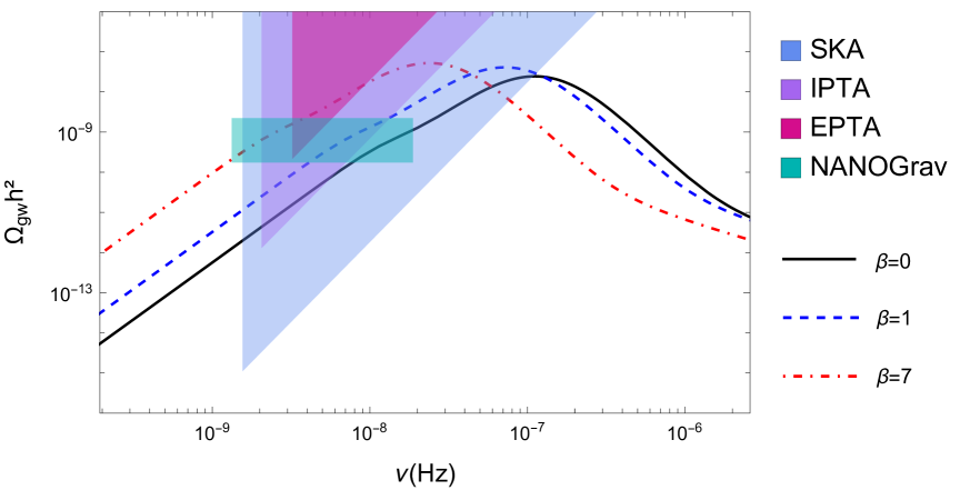
Figure 5: The SGWB energy spectra from three sources in QCD phase transition as a function of frequency with different values of GUP parameter $\beta$.

VI Conclusion

In this work, we have investigated the SGWB generated from a first-order cosmological QCD phase transition within the framework of a new GUP (1). We systematically derived the higher-order GUP corrections to the SGWB spectrum, emphasizing the distinctions and physical implications arising from positive and negative deformation parameters. Our analysis demonstrates that only positive GUP parameters yield physically consistent and observationally viable gravitational wave signals, characterized by a notable shift in the SGWB peak toward lower frequencies and a modest enhancement in energy density as the GUP parameter increases. These modifications play a crucial role in understanding the quantum gravity effects during the cosmological evolution. Furthermore, we evaluated the detectability of these modified SGWB signals using current and forthcoming pulsar timing array experiments, such as SKA, IPTA, EPTA, and NANOGrav. Our results reveal that these facilities possess sufficient sensitivity to potentially detect QG corrected gravitational wave signals. Hence, our study not only provides new insights into the interaction between the effects of QG and cosmological phase transitions, but also highlights the promising potential of gravitational wave astronomy as a powerful tool for exploring and testing Planck-scale QG theories.