On the exact solutions of a two-dimensional hydrogen atom in a constant magnetic field

Abstract

We discuss the exact polynomial solutions for the two-dimensional hydrogen atom in a constant magnetic field already studied earlier by other authors. In order to provide a suitable meaning for such solutions we compare them with numerical results provided by the Rayleigh-Ritz method.

1 Introduction

There are many exactly-solvable quantum-mechanical models. The most popular an useful ones may be the harmonic oscillator and the hydrogen atom that are discussed in any textbook on quantum mechanics[1] and quantum chemistry[2]. Several years ago, Flessas and collaborators[3, 4, 5, 6, 7] discovered that some quantum-mechanical models that are not exactly solvable admit some exact solutions for particular values of the model parameters. This kind of problems are now known as quasi solvable (QS) or conditionally solvable and have been widely studied[8]. Several researchers thought that the QS solutions are the exact solutions of the quantum-mechanical models and derived incorrect conclusions from them as discussed elsewhere[9, 10]. In fact, such QS solutions are of scarce utility if one is not able to connect them with the actual solutions of the quantum-mechanical models[9, 10] (see, for example, the enlightening papers by Child et al[11] and Le et al[12]).

Recently, Bildstein and Grabowski[13] proposed a generalization of the Frobenius method and applied it to quantum-mechanical models with polynomial potentials in one, two and three dimensions. They obtained analytical solutions for most of them. In particular, they considered in detail the two-dimensional hydrogen atom in a constant magnetic field already studied by Le et al[12] and somewhat earlier by Taut[14]. In particular, Turbiner and Escobar Ruiz discussed the existence of a hidden algebra. The purpose of this paper is the interpretation of the exact QS solutions for this model.

In section 2 we outline some relevant features of the Schrödinger equation for the two-dimensional hydrogen atom in a constant magnetic field. In section 3 we derive some exact analytical solutions by means of the Frobenius method and a simple truncation rule already used in earlier papers[9, 10]. In order to provide a sound interpretation of the analytical QS results, in section 4 we compare them with numerical results coming from the well known Rayleigh-Ritz method (RRM)[2] that yields increasingly accurate upper bounds to the actual eigenvalues of the Schrödinger equation[16, 17]. Finally, in section 5 summarize the main results and draw conclusions.

2 The model

The Schrödinger equation for the two-dimensional hydrogen atom in a constant magnetic field is separable in polar coordinates and the resulting radial eigenvalue equation in atomic units is[12]

$$\left[-\frac{1}{2}\left(\partial_{r}^{2}+\frac{1}{r}\partial_{r}\right)+\frac{m^{2}}{2r^{2}}+\frac{\gamma^{2}}{8}r^{2}-\frac{Z}{r}\right]R(r)=WR(r),\;W=E-\frac{\gamma m}{2},$$ (1)

where $E$ is the energy and $m=0,\pm 1,\pm 2,\ldots$ is the magnetic quantum number. This equation is a particular case of a more general one studied in our earlier paper[9]. Bound states are solutions of this eigenvalue equation that are square integrable

$$\int_{0}^{\infty}R(r)^{2}r\,dr<\infty.$$ (2)

Such solutions are possible only for discrete values of $W$ that we may denote $W_{\nu s}\left(Z,\gamma\right)$, where $s=|m|$ and $\nu=0,1,\ldots$ is the radial quantum number (the number of nodes of $R(r)$ in the interval $0<r<\infty$). The corresponding square-integrable solutions are $R_{\nu s}(r)$. It is well known that $W_{\nu s}>W_{\nu^{\prime}s}$ if $\nu>\nu^{\prime}$ and $W_{\nu s}>W_{\nu s^{\prime}}$ if $s>s^{\prime}$.

It is clear that if $\gamma^{2}>0$ then there are bound states for all $-\infty<Z<\infty$. From now on we only consider $Z>0$ that is consistent with the physical model. According to the Hellmann-Feynman theorem (HFT)[18, 19]

$$\frac{\partial W_{\nu s}}{\partial Z}=-\left\langle\frac{1}{r}\right\rangle<0,\;\frac{\partial W_{\nu s}}{\partial\gamma}=\frac{\gamma}{4}\left\langle r^{2}\right\rangle>0,\;\gamma>0,$$ (3)

we conclude that the eigenvalues decrease with $Z$ and increase with $\gamma$. For $\gamma=0$ all the eigenvalues are negative

$$W_{\nu s}\left(Z,0\right)=-\frac{2Z^{2}}{\left(2\nu+2s+1\right)^{2}},$$ (4)

while for $Z=0$ they are positive

$$W_{\nu s}\left(0,\gamma\right)=\frac{1}{2}\left(2\nu+s+1\right)\gamma.$$ (5)

Therefore, as $\gamma$ increases the eigenvalues $W_{\nu s}\left(Z,\gamma\right)$ become positive and there exist $\gamma=\gamma_{\nu s}^{c}$ such that $W_{\nu s}=0$. These critical values of $\gamma$ satisfy $\gamma_{\nu s}^{c}<\gamma_{\nu^{\prime}s}^{c}$ if $\nu>\nu^{\prime}$ and $\gamma_{\nu s}^{c}<\gamma_{\nu s^{\prime}}^{c}$ if $s>s^{\prime}$.

By means of a suitable change of variables[20] we may set either $|Z|=1$ or $\gamma=1$ (preferably $\gamma=2$ in order to derive an equation similar to that studied in our earlier paper[9]). However, here we will keep both model parameters in order to compare present results with those of Bildstein and Grabowski[13].

The analytical results outlined above may appear to be rather trivial and well known. We decided to show them here because most of them have been overlooked by the researchers who drawn incorrect conclusions from the exact polynomial solutions of QS models as discussed in our earlier paper[9] (se allso[10] )

3 Exact polynomial solutions

In this section we will derive exact solutions to the eigenvalue equation (1) by means of the standard Frobenius method used in our earlier paper[9] (in fact, Taut[14] had used it several years before). On taking into account the asymptotic behaviour of $R(r)$ at origin $R(r)\sim r^{s}$ and at infinity $R(r)\sim e^{-\gamma r^{2}/4}$, we propose an ansatz of the form

$$R(r)=r^{s}e^{-\gamma r^{2}/4}\sum_{j=0}^{\infty}c_{j}r^{j}.$$ (6)

The expansion coefficients $c_{j}$ satisfy the three-term recurrence relation (TTRR)

$$c_{j+2} = A_{j}c_{j+1}+B_{j}c_{j},\;j=0,1,\ldots,$$

$$A_{j} = -\frac{2Z}{\left(j+2\right)\left(j+2\left(s+1\right)\right)},\;B_{j}=\frac{\gamma\left(j+s+1\right)-2W}{\left(j+2\right)\left(j+2\left(s+1\right)\right)}.$$ (7)

In order to obtain an exact polynomial solution of degree $n$ we require that $c_{n}\neq 0$ and $c_{n+1}=c_{n+2}=0$, $n=0,1,\ldots$, so that $c_{j}=0$ for all $j>n.$ These conditions lead to $B_{n}=0$ from which we obtain

$$W=W_{s}^{(n)}=\frac{\gamma\left(n+s+1\right)}{2},$$ (8)

and

$$B_{j}=\frac{\gamma\left(j-n\right)}{\left(j+2\right)\left(j+2\left(s+1\right)\right)}.$$ (9)

It only remains to solve the condition $c_{n+1}=0$ for either $Z$ or $\gamma$. Here, we follow Bildstein and Graboski[13] (who had followed Le at al[12]) and solve for $\gamma$ though solving for $Z$ is perhaps more convenient[9, 10]. In any case, the exact polynomial solutions may be written as

$$R_{s}^{(n)}(r)=r^{s}e^{-\gamma r^{2}/4}\sum_{j=0}^{n}c_{js}^{(n)}r^{j},$$ (10)

but for simplicity we will write $c_{j}$ for the expansion coefficients in what follows.

Before proceeding with the calculations note that $W_{s}^{(n)}$ is positive for all values of $n$, $s$ and $\gamma$ so that the exact polynomial solutions cannot provide information on the whole spectrum of the problem. Besides, $n$ is not the radial quantum number as shown below. Many researchers wrongly interpreted $W_{s}^{(n)}$ as the spectrum of the problem and $n$ as the radial quantum number as argued in earlier papers[9, 10].

When $n=0$ we have

$$c_{1}=-\frac{2Z}{2s+1}.$$ (11)

The only solution for $c_{1}=0$ is $Z=0$ and we obtain a set of exact solutions for the harmonic oscillator

$$W_{s}^{(0)}=W_{0s}=\frac{\gamma(s+1)}{2},\;R_{s}^{(0)}(r)=R_{0s}(r)=c_{0}r^{s}e^{-\gamma r^{2}/4}.$$ (12)

Note that $\gamma$ is arbitrary because the harmonic oscillator is exactly solvable for all values of this parameter.

When $n=1$ the second and third coefficients are

$$c_{1}=-\frac{2Z}{2s+1},\;c_{2}=\frac{Z^{2}}{(s+1)(2s+1)}-\frac{\gamma}{4(s+1)},$$ (13)

from which we obtain

$$\gamma=\frac{4Z^{2}}{2s+1},$$ (14)

and

$$W_{s}^{(1)}=\frac{2(s+2)Z^{2}}{2s+1},\;R_{s}^{(1)}(r)=c_{0}r^{s}e^{-\gamma r^{2}/4}\left(1-\frac{2Zr}{2s+1}\right).$$ (15)

We appreciate that the truncation method fails to provide the solutions without nodes for $Z>0$, a fact that was pointed out by Taut[14] many years ago.

When $n=2$ the termination condition is

$$c_{3}=\frac{z\left[\gamma\left(4s+3\right)-2z^{2}\right]}{3\left(s+1\right)\left(2s+1\right)\left(2s+3\right)}=0.$$ (16)

When $Z=0$ we obtain the solutions of the harmonic oscillator with one node

$$W_{s}^{(2)}=W_{1s}=\frac{\gamma(s+3)}{2},\;R_{s}^{(2)}(r)=R_{1s}(r)=c_{0}r^{s}e^{-\gamma r^{2}/4}\left[1-\frac{\gamma r^{2}}{2\left(s+1\right)}\right].$$ (17)

If we solve equation (16) for $\gamma$ we have

$$\gamma=\frac{2Z^{2}}{4s+3},$$ (18)

and

$$W_{s}^{(2)}=\frac{Z^{2}(s+3)}{4s+3},\;R_{s}^{(2)}(r)=c_{0}r^{s}e^{-\gamma r^{2}/4}\left[1-\frac{2Zr}{2s+1}+\frac{2Z^{2}r^{2}}{\left(2s+1\right)\left(4s+3\right)}\right].$$ (19)

The truncation method yields a solution $R_{s}^{(2)}(r)$ with two nodes and fails to provide those with zero and one node. Le et al[12] proved a most remarkable theorem on the nodes of the exact polynomial solutions.

These results agree with those derived by Bildstein and Grabowski who also showed expressions for $n=3$. The most important point here is that Bildstein and Grabowski did not mention that $W_{s}^{(n)}(Z)$ are not the eigenvalues of the radial equation (1) which is the reason why they do not exhibit the correct behaviour with respect to $Z$ (see equation (3)). The behaviour of $W_{\nu s}(Z)$ with respect to $Z$ has already been discussed in two earlier papers[9, 10] and the limitations of the exact polynomial solutions have been discussed by Taut[14] and Le et al[12]. A suitable interpretation of the QS results is most important as argued in earlier papers[9, 10].

Here, we derive two general results. First, since $B_{j}$ is a linear function of $\gamma$ and $A_{j}$ does not depend on this parameter, then if $c_{j}$ is a polynomial function of $\gamma$ of degree $k$ then $c_{j+2}$ is a polynomial function of this parameter of degree $k+1$. Consequently, for $n>0$ we obtain a set of roots $\gamma_{s}^{(n,i)}$, $i=1,2,\ldots,k_{n}$, where $k_{2n}=k_{2n-1}=n$, $n=1,2,\ldots$. This result was already derived by Le et al[12] in a somewhat different way. The corresponding QS eigenvalues $W_{s}^{(n,i)}=W_{s}^{(n)}\left(\gamma_{s}^{(n,i)}\right)$ are associated to the eigenfunctions $R_{s}^{(n,i)}(r)$ with expansion coefficients $c_{js}^{(n,i)}$.

Second, if we substitute $\gamma=\xi Z^{2}$ and $c_{j}=d_{j}Z^{j}$ in the recurrence relation (7) with $B_{j}$ given by (9) we obtain the TTRR

$$d_{j+2}=-\frac{2}{\left(j+2\right)\left(j+2\left(s+1\right)\right)}d_{j+1}+\frac{\xi\left(j-n\right)}{\left(j+2\right)\left(j+2\left(s+1\right)\right)}d_{{j}},$$ (20)

that is exactly the TTRR relation (7) with $Z=1$. We thus conclude that $\gamma_{s}^{(n)}(Z)=\gamma_{s}^{(n)}(1)Z^{2}$ and $c_{j}(Z)=c_{j}(1)Z^{j}$. It is obvious that we can set $Z=1$ without loss of generality.

In the next section we provide an interpretation of the QS results as was done by Le et al[12]. In closing this section, we just mention that $A_{j}=0$ for all $j$ when $Z=0$ in which case we obtain the two-term recurrence relation for the harmonic oscillator $c_{2j+2}=B_{2j}c_{2j}$ because $c_{2j+1}=0$ for all $j$.

4 Variational calculation

One way of providing a suitable interpretation of the QS results is to compare them with accurate numerical eigenvalues for an interval of the chosen model parameter. Le et al[12] resorted to an approach based on the iterative solution of the secular equation[21] already proposed earlier by other authors[22]. In this section, we carry out some numerical calculations based on the RRM[2] that is known to provide increasingly tighter upper bounds to the exact eigenvalues[16, 17]. For simplicity, we choose the non-orthogonal basis set

$$u_{is}(r)=e^{i+s}e^{-\gamma r^{2}/4},\;i=0,1,\ldots,$$ (21)

that is suitable for sufficiently large values of $\gamma$. The equations of the RRM with a non-orthogonal basis set are well known[2, 23] and will not be shown here. For concreteness, we restrict our calculations to $Z=1$ and $s=0$.

Tables 1 and 2 show the convergence of the RRM eigenvalues for $\gamma=4$ and $\gamma=2/3$, respectively, as the dimension $N$ of the basis set increases. The RRM yields the exact QS results $W_{10}=W_{0}^{(1)}=4$ in the former case and $W_{20}=W_{0}^{(2)}=1$ in the latter. This fact was already pointed out by Le et al[12] but we can show it more clearly in terms of present approach. In fact, the secular determinants $D_{N}$ for $N=2$ and $N=3$ exhibit the exact results

$$D_{2} = \frac{4-\pi}{128}\left(W-4\right)\left[W-\frac{2\sqrt{2}\left(\sqrt{\pi}-\sqrt{2}\right)}{\pi-4}\right],$$

$$D_{3} = \frac{81}{128}\left(W-1\right)\left[9\left(5\pi-16\right)W^{2}+6\left(3\sqrt{3}\pi^{\frac{3}{2}}-6\pi-10\sqrt{3}\sqrt{\pi}+20\right)W\right.$$ (22)

$$\left.-2\sqrt{3}\pi^{\frac{3}{2}}-11\pi+10\sqrt{3}\sqrt{\pi}+24\right].$$

It also follows from Tables 1 and 2 that the truncation approach is unable to provide the ground state $W_{00}(\gamma)$ as argued in the preceding section and as was pointed out several years ago by Taut[14].

Figure1 shows RRM eigenvalues $W_{\nu 0}(\gamma)$, $\nu=0,1,2,3$, and QS eigenvalues $W_{0}^{(n)}(\gamma)$ for $n=0,1,\ldots,6$. We appreciate that every point $\left[\gamma_{s}^{(n,i)},W_{0}^{(n,i)}\right]$ marks an intersection between a pair of curves $W_{\nu 0}(\gamma)$ and $W_{0}^{(n)}(\gamma)$. However, there are intersections between curves $W_{\nu 0}(\gamma)$ and $W_{0}^{(n)}(\gamma)$ that do not correspond to points $\left[\gamma_{s}^{(n,i)},W_{0}^{(n,i)}\right]$. This figure provides a clear interpretation of the QS results. Le et al[12] resorted to somewhat different plots for the same purpose. On the other hand, Bildstein and Grabowski[13] did not attempt to provide such interpretation which is necessary to avoid the mistakes mentioned above.

The rate of convergence of the RRM with the basis set (21) decreases as $\gamma$ decreases. For small values of $\gamma$, say $\gamma<1$, it is convenient to resort to the alternative basis set

$$v_{is}(r)=e^{i+s}e^{-\alpha r},\;i=0,1,\ldots,$$ (23)

where $\alpha$ is an adjustable parameter. One obtains the greatest rate of convergence when $\alpha$ is determined variationally but here we just choose $\alpha=1$ in all our calculations because we do not need high accuracy.

Figure 2 shows the QS eigenvalues $W_{0}^{(n)}(\gamma)$, $n=0,1,\ldots,8$, and the RRM ones $W_{\nu 0}$, $\nu=1,2,\ldots,5$, in an interval of values of $\gamma$ closer to the origin. The conclusions are similar to those drawn from Figure 1.

Although at first sight the critical values of $\gamma$ do not appear to be related with the analysis of the QS results, it is clear that the truncation approach cannot provide any information about the actual eigenvalue $W_{\nu s}$ when $\gamma<\gamma_{\nu s}^{c}$. For this reason, we have decided to calculate some critical values of $\gamma$. Table 3 shows values of $\gamma_{\nu s}^{c}$ for $s=0$ and $\nu=0,1,\ldots,9$. In order to obtain them we simply set $W=0$ in the RRM secular equation and solved for $\gamma$. We also resorted to the Riccati-Padé method[24] in order to obtain more accurate results in some cases. Taking into account figures 1 and 2 and the extremely large value of $\gamma_{00}^{c}$ we understand why the QS results fail to include the ground state of the model.

5 Further comments and conclusions

Bildstein and Grabowski[13] derived some isolated exact solutions of the eigenvalue equation (1) by means of a truncation procedure used earlier by other authors[14, 12, 9, 10] but did not try to connect them with the actual eigenvalues and eigenfunctions. The correct interpretation of the QS solutions is most important in order to avoid the mistakes discussed elsewhere[9, 10]. For this reason we decided to carry out present analysis which was presented in a way that slightly differs from those of Taut[14] and Le et al[12].

Table 1: Lowest RRM eigenvalues for $Z=1$, $s=0$ and $\gamma=4$

$N$	$\nu=0$	$\nu=1$	$\nu=2$	$\nu=3$
4	-1.449885589	4	8.34525977	17.66452696
5	-1.458156835	4	8.344361267	12.69095166
6	-1.459389343	4	8.344349784	12.53313314
7	-1.459560848	4	8.344349441	12.53290257

Table 2: Lowest RRM eigenvalues for $Z=1$, $s=0$ and $\gamma=\frac{2}{3}$

$N$	$\nu=0$	$\nu=1$	$\nu=2$	$\nu=3$
4	-1.835656791	0.184392123	1	1.904674543
5	-1.935195212	0.181236739	1	1.743664442
6	-1.968131654	0.1807724337	1	1.743410741
7	-1.976985355	0.1807106702	1	1.743408135

Table 3: Some critical values of the parameter $\gamma$

$\nu$	$\gamma^{c}_{\nu 0}$
0	9.399451214
1	0.4484067794
2	0.09870506669
3	0.03616422276
4	0.01705321756
5	0.005668542649
6	0.003691507495
7	0.002536579450
8	0.001817259637
9	0.001024706586

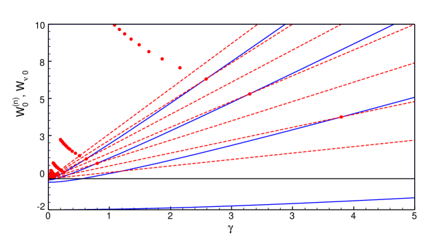
Figure 1: RRM eigenvalues $W_{\nu 0}$, $\nu=0,1,2,3$ (blue continuous lines), TTRR eigenvalues $W^{(n)}_{0}(\gamma)$, $n=0,1,\ldots,6$ (red dashed lines) and $W^{(n)}_{0}\left(\gamma^{(n)}_{0}\right)$ (red points)

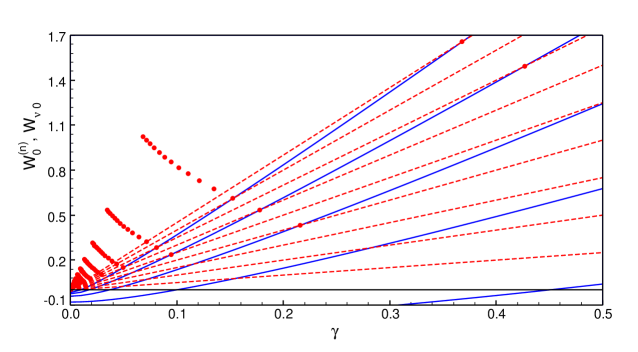
Figure 2: RRM eigenvalues $W_{\nu 0}$, $\nu=1,2,\ldots,5$ (blue continuous lines), TTRR eigenvalues $W^{(n)}_{0}(\gamma)$, $n=0,1,\ldots,8$ (red dashed lines) and $W^{(n)}_{0}\left(\gamma^{(n)}_{0}\right)$ (red points)

References

- [1] C. Cohen-Tannoudji, B. Diu, and F. Laloë, Quantum Mechanics (John Wiley & Sons, New York, 1977).
- [2] F. L. Pilar, Elementary Quantum Chemistry (McGraw-Hill, New York, 1968).
- [3] G. P Flessas, Phys. Lett. A 72, 289 (1979).
- [4] G. P Flessas and K. P. Das, Phys. Lett. A 78, 19 (1980).
- [5] G. P Flessas, J. Phys. A 14, L209 (1981).
- [6] G. P Flessas, Phys. Lett. A 81, 17 (1981).
- [7] G. P Flessas and A. Watt, J. Phys. A 14, L315 (1981).
- [8] A. V. Turbiner, Phys. Rep. 642, 1 (2016). arXiv:1603.02992 [quant-ph].
- [9] F. M. Fernández, Ann. Phys. 434, 168645 (2021). arXiv:2109.11545 [quant-ph]
- [10] P. Amore and F. M. Fernández, J. Math. Phys. 62, 032106 (2021). arXiv:2110.14526 [quant-ph]
- [11] M. S. Child, S-H. Dong, and X-G. Wang, J. Phys. A 33, 5653 (2000).
- [12] D-N. Le, N-T. D. Ngoc-Tram D. Hoang, and V-H. Le, J. Math. Phys. 58, 042102 (2017).
- [13] S. Bildstein and M. Grabowski, J. Math. Phys. 66, 012103 (2025).
- [14] M. Taut, J. Phys. A 28, 2081 (1995).
- [15] A. V. Turbiner and Escobar-Ruiz M. A., J. Phys. A 46, 295204 (2013).
- [16] J. K. L. MacDonald, Phys Rev. 43, 830 (1933).
- [17] F. M. Fernández, J. Math. Chem. 63, 911 (2025). arXiv:2206.05122 [quant-ph]
- [18] P. Güttinger, Z. Phys. 73, 169 (1932).
- [19] R. P. Feynman, Phys. Rev. 56, 340 (1939).
- [20] F. M. Fernández, Dimensionless equations in non-relativistic quantum mechanics, arXiv:2005.05377 [quant-ph].
- [21] N-T. Hoang-Do, D-L. Pham, and V-H. Le, Physica B 423, 31 (2013).
- [22] F. M. Fernández, A. M. Mesón, and E. A. Castro, J. Phys. A 18, 1389 (1985).
- [23] F. M. Fernández, J. Math. Chem. 62, 2083 (2024). arXiv:2405.10340 [quant-ph]
- [24] F. M. Fernández, Q. Ma, and R. H. Tipping, Phys. Rev. A 39, 1605 (1989).