The Subtle Interplay between Square-root Impact,
Order Imbalance & Volatility: A Unifying Framework

Abstract

In this work, we aim to reconcile several apparently contradictory observations in market microstructure: is the famous “square-root law” of metaorder impact, which decays with time, compatible with the random-walk nature of prices and the linear impact of order imbalances? Can one entirely explain the volatility of prices as resulting from the flow of uninformed metaorders that mechanically impact them? We introduce a new theoretical framework to describe metaorders with different signs, sizes and durations, which all impact prices as a square-root of volume but with a subsequent time decay. We show that, as in the original propagator model, price diffusion is ensured by the long memory of cross-correlations between metaorders. In order to account for the effect of strongly fluctuating volumes $q$ of individual trades, we further introduce two $q$-dependent exponents, which allow us to describe how the moments of generalized volume imbalance and the correlation between price changes and generalized order flow imbalance scale with $T$. We predict in particular that the corresponding power-laws depend in a non-monotonic fashion on a parameter $a$, which allows one to put the same weight on all child orders or to overweight large ones, a behaviour that is clearly borne out by empirical data. We also predict that the correlation between price changes and volume imbalances should display a maximum as a function of $a$, which again matches observations. Such noteworthy agreement between theory and data suggests that our framework correctly captures the basic mechanism at the heart of price formation, namely the average impact of metaorders. We argue that our results support the “Order-Driven” theory of excess volatility, and are at odds with the idea that a “Fundamental” component accounts for a large share of the volatility of financial markets.

1 Introduction

Price impact refers to the fact that buyers push the price up and sellers push the price down [1, 2]. The traditional Efficient Market interpretation of this empirical fact is that buyers and sellers are on average informed, and lo and behold, the price moves according to their prediction [3, 4]. This scenario is at the heart of the celebrated Kyle model for price impact [5].

Another, very different interpretation of price impact is that it is a purely statistical reaction of the market to incoming order flow, where information plays little role. Prices move simply because people trade, whatever the reason they are trading, and volatility is the result of people randomly buying and selling. This is the Order-Driven view of markets, explicitly spelled out in [2], chapter 20 – but see also [6, 7, 1] and in a different setting, [8, 9]. In this scenario, there is no “information revelation” but rather “self-fulfilling prophecies”, as emphasized in [10, 11].

Of course, reality should lie somewhere between these two extremes. There are surely some informed trades, and news do impact prices, but there is also overwhelming evidence for the presence of “noise traders”, excess trading and excess volatility in financial markets, see e.g. [12, 13, 14, 15, 16]. Direct empirical estimates suggest that informed trades are a minority (see [17] and [2], chapter 16). While we are convinced that the Order-Driven view is a much closer approximation to the dynamics of markets, there are several empirical loose ends that need to be tied up. A major issue is how to reconcile two prominent stylized facts of market microstructure, namely, (i) the long-range memory in order signs (i.e. $+1$ for buy orders and $-1$ for sell orders) and (ii) the ubiquitous square-root law of market impact (that governs the average price move induced by the execution of a sequence of orders) with the random walk nature of prices, with a volatility $\sigma$ that is directly proportional to the amplitude of the square-root law. More precisely, the square-root law states that the average price impact $\mathcal{I}$ of a metaorder of total volume $Q$ is given by

$$\mathcal{I}(Q)=Y\sigma\sqrt{\frac{Q}{\phi}},$$ (1)

where $Y$ is a $O(1)$ numerical coefficient and $\phi$ is the average flow of orders executed in the market per unit time – see e.g. [18, 19, 20, 21, 22, 23, 24, 25, 26, 27, 28] and [2, 29] for reviews.

Eq. (1) may look familiar, and in fact trivial: superficially, it states that price changes (i.e. $\mathcal{I}(Q)$) grow as the square-root of execution time $T$, i.e. the law of random walks, provided one assumes that $T$ and $Q$ are proportional. But, as argued in [30], such an argument is completely misleading: not only $\mathcal{I}(Q)$ is an average price change and not a standard deviation; but also $\mathcal{I}(Q)$ is found to depend only on the quantity executed $Q$ and not on execution time $T$. Furthermore, it is known that the impact of metaorders decays, on average, after the end of the execution period (e.g. [31, brokmann2015slow, 25]). Note that all these features are at odds with the Kyle model that predicts linear and permanent impact, resulting from information revelation [5].

We are thus confronted with three interrelated but separate problems:

• (a) What is the basic mechanism that explains the square-root law, Eq. (1), and its surprising universal character?

• (b) Can the volatility of prices $\sigma$ be explained only in terms of the impact of intertwined, possibly uninformed metaorders? Or is it impact that is somehow slaved to some “Fundamental” volatility?

• (c) Can one reconcile the square-root law for metaorders with a linear relation between average price changes and order flow imbalance?

Although many theories have been proposed to explain the square-root law, there is no consensus on the issue. The Latent Liquidity Theory proposed in [33] (see also [34, 2]) seems to capture many features observed in data but seems inconsistent with others, in particular those reported in the recent paper of Maitrier et al. [35]. We will not attempt to dwell further on this particular issue here but accept it as an incontrovertible empirical fact, still waiting for a fully convincing explanation. We will rather focus on points (b) and (c) above: knowing that the duration of metaorders is power-law distributed, can one reconcile the square-root impact law with the volatility of markets and with a locally linear aggregate impact law?

In order to answer these questions quantitatively, we introduce in section 2 a new theoretical framework to describe metaorders with different signs, sizes and durations, which impact prices as a square-root of volume but with a subsequent time decay. We show in section 4 that, as in the original propagator model, price diffusion is ensured by the long memory of cross-correlations between metaorders. In order to account for the effect of strongly fluctuating volumes $q$ of individual trades, we need to further introduce two $q$-dependent exponents, which we justify empirically and allow us to account for the way the moments of generalized volume imbalance (section 3) and the correlation between price changes and generalized volume imbalance (section 5) scales with $T$. We predict in particular that the corresponding power-laws depend in a non-monotonic fashion on a parameter $a$ that allows one to put the same weight on all child orders or overweight large orders, a behaviour clearly borne out by empirical data (section 5). We also predict that the correlation between price changes and volume imbalances should display a maximum as a function of $a$, which again matches observations (section 5). We conclude by arguing that our results support the “Order-Driven” theory of markets, and are at odds with the idea that a “Fundamental” component accounts for a large share of the volatility of financial markets.

2 A continuous time description of order flow

2.1 Model set-up

We posit that between $t$ and $t+{\rm d}t$ and with probability $\nu{\rm d}t$ a new metaorder of random sign $\varepsilon(t)=\pm 1$ and duration $s(t)$ is initiated. The volume of child orders is $q$ (which might itself be random, see below), and during execution the probability that one of them gets executed is $\varphi{\rm d}t$, independently of the size $q$. We neglect throughout this paper activity fluctuations as well as intraday seasonalities, as these are not crucial for the effects we want to focus on. This means that $\mu,\varphi$ and the average duration $\bar{s}$ are chosen to be time independent.

The total size of the metaorder is thus $Q=q\varphi s+O(\sqrt{s})$. The probability density of durations $s$ is denoted $\Psi(s)$, which will typically has a power-law tail $\Psi(s)\propto s^{-1-\mu}$, such that the distribution of metaorder sizes $Q$ inherits from this power-law, and decays as $Q^{-1-\mu}$ as suggested by empirical data [36, 37].

Such a power-law distribution of metaorder sizes is the basic mechanism proposed by Lillo, Mike and Farmer (LMF) [38] to explain the long memory of order signs, which is known to decay with lag $\tau$ as $\tau^{-\gamma}$ with $0<\gamma<1$ [10]. Within the LMF model, one has $\gamma=\mu-1$, a result recently validated in great details by Sato and Kanazawa [37] using data from the Tokyo Stock Exchange. In a later stage, we will allow the exponent $\mu$ to depend on $q$, to account for the fact that large child orders tend to be less autocorrelated that small ones.

We will also allow the sign of different metaorders to be correlated, as indeed observed in data [23, 39]. More precisely, we will model the long-term decay of the autocorrelation of signs, $\mathbb{E}[\varepsilon(t)\varepsilon(t+\tau)]$ as a power-law $\tau^{-\gamma_{\times}}$, with an exponent $\gamma_{\times}$ a priori such that $\gamma_{\times}\geq\gamma$ such not to contradict the LMF hypothesis.

We start warming up by computing two simple quantities, the total number of active metaorders and the average trading volume within a window of duration $T$. We will then turn to the distribution of volume imbalance in windows of different sizes.

2.2 Average number of metaorders

The total number of metaorders $N_{T}$ that are active between $t=0$ and $t=T$ is given by

$$N_{T}=\int_{-\infty}^{T}{\rm d}N_{t}\,\,\mathbb{I}(t+s(t)>0),$$ (2)

where ${\rm d}N_{t}=0$ if there is no new metaorder initiated between $t$ and $t+{\rm d}t$ and ${\rm d}N_{t}=1$ otherwise. This equation means that to be active in $[0,T]$, it must start before $t=T$ and end at least after $t=0$.

The average over the probability of initiating metaorders and over their duration gives

$$\overline{N}_{T}=\nu\int_{-\infty}^{T}{\rm d}t\int_{0}^{\infty}{\rm d}s\,\Psi(s)\,\mathbb{I}(t+s>0)=\nu(T+\bar{s}),$$ (3)

where we assume henceforth that the average size of metaorders is finite, i.e. $\bar{s}:=\int_{0}^{\infty}{\rm d}s\,s\Psi(s)<+\infty$, which is tantamount to $\mu>1$. Hence, for large $T\gg\bar{s}$, one finds $\overline{N}_{T}\approx\nu T$, as expected.

In the following, we will always make averages over the metaorder initiation process, and often replace ${\rm d}N_{t}$ by $\nu{\rm d}t$ whenever possible. When comparing with empirical data, we will work in trade time $N_{T}$ but still call this quantity $T$. Translating our results is real time is, however, non-trivial because, as is well known, the activity rate $\nu$ shows strongly intermittent dynamics (often modeled using Hawkes processes, see e.g. [2], chapter 9) on top of a U-shaped intraday pattern.

2.3 Average trading activity and trading volume

Second warm-up question: what is the total activity $A_{T}$ and total trading volume $V_{T}$ executed between $t=0$ and $t=T$? In the following we assume that all child orders have the same size and denote $\kappa:=q\varphi\nu$, so that activity and trading volume are simply related by $\overline{V}_{T}=q\overline{A}_{T}$. More generally, the following results holds with $\kappa=\bar{q}\varphi\nu$.

There are two terms, corresponding to metaorders initiated within the period $[0,T]$ or before $t=0$ that are still active in $[0,T]$. We denote these two terms as $V_{T}^{1}$ and $V_{T}^{2}$, with

$$V_{T}^{1}=\int_{0}^{T}{\rm d}N_{t}\left[\mathbb{I}(t+s(t)>T)q\varphi(T-t)+\mathbb{I}(t+s(t)<T)q\varphi s\right],$$ (4)

which after averaging over ${\rm d}N_{t}$ gives

$$V_{T}^{1}=\kappa\int_{0}^{T}{\rm d}t\left[\mathbb{I}(t+s(t)>T)(T-t)+\mathbb{I}(t+s(t)<T)s\right].$$ (5)

Similarly, for $V_{T}^{2}$ we get

$$V_{T}^{2}=\kappa\int_{-\infty}^{0}{\rm d}t\left[\mathbb{I}(t+s(t)>T)T+\mathbb{I}(0<t+s(t)<T)(s(t)+t)\right]$$ (6)

Now let us compute the average over duration $s$, given by

$$\overline{V}_{T}^{1}=\kappa\int_{0}^{T}{\rm d}t\int_{0}^{\infty}{\rm d}s\,\Psi(s)\left[\mathbb{I}(t+s>T)(T-t)+\mathbb{I}(t+s<T)s\right]$$ (7)

and

$$\overline{V}_{T}^{2}=\kappa\int_{-\infty}^{0}{\rm d}t\int_{0}^{\infty}{\rm d}s\,\Psi(s)\left[\mathbb{I}(t+s>T)T+\mathbb{I}(0<t+s<T)(s+t)\right]$$ (8)

Carefully taking the derivative with respect to $T$ one finds:

$$\frac{\partial\overline{V}_{T}^{1}}{\partial T}=\kappa\left[\int_{0}^{T}{\rm d}s\,s\Psi(s)+T\int_{T}^{\infty}{\rm d}s\,\Psi(s)\right];\qquad\frac{\partial\overline{V}_{T}^{2}}{\partial T}=\kappa\int_{T}^{\infty}{\rm d}s\,(s-T)\Psi(s).$$ (9)

Hence, the total average executed volume $\overline{V}_{T}=\overline{V}_{T}^{1}+\overline{V}_{T}^{2}$ is given, for large $T$, by

$$\overline{V}_{T}=\kappa\bar{s}T\approx q\varphi\bar{s}\,\overline{N}_{T},$$ (10)

i.e. the average volume per metaorder $\overline{Q}=q\varphi\bar{s}$ times the average number of metaorders $\overline{N}_{T}$. So in this model the average volume flow per unit time is $\phi:=\nu\overline{Q}=\kappa\bar{s}$. Note that for large enough $T$ it is dominated by $V_{T}^{1}$.

The average activity (i.e. number of trades per unit time) is given by $\nu\varphi\bar{s}$. We will denote its inverse $\tau_{0}:=(\nu\varphi\bar{s})^{-1}$, which is the average time between two trades. Finally, note that the average number of child orders per metaorder is $\bar{n}:=\varphi\bar{s}$.

3 Order Flow Imbalance

In this section we compute, within our model, the statistics of the flow imbalance during periods of duration $T$. In the case where all trades have the same size $q$, volume imbalance is trivially proportional to sign imbalance. It turns out that due to the heavy tail in metaorder durations, sign imbalance scales anomalously with $T$ and has non-Gaussian fluctuations, even when the signs of metaorders are independent.

When single trade volumes are themselves strongly fluctuating, the statistics of volume imbalance can be very different from those of sign imbalance, a feature we actually observe on data and reproduce within our framework – see section 3.2 below.

3.1 Sign Imbalance

The sign imbalance $I^{0}_{T}$ in an interval of size $T$ is given by a sum of two contributions, as for the traded volume above:

$$I^{0}_{T,1}=\varphi\int_{0}^{T}\varepsilon(t){\rm d}N_{t}\left[\mathbb{I}(t+s(t)>T)(T-t)+\mathbb{I}(t+s(t)<T)s\right],$$ (11)

and

$$I^{0}_{T,2}=\varphi\int_{-\infty}^{0}\varepsilon(t){\rm d}N_{t}\left[\mathbb{I}(t+s(t)>T)T+\mathbb{I}(0<t+s(t)<T)(s(t)+t)\right].$$ (12)

Because $\mathbb{E}[\varepsilon(t)]=0$, these terms are of mean zero. In this subsection and the next, we assume metaorders to be independent, in particular one has $\mathbb{E}[\varepsilon(t){\rm d}N_{t}\varepsilon(t^{\prime}){\rm d}N_{t^{\prime}}]=\delta(t-t^{\prime}){\rm d}N_{t}$.

The sign imbalance variance is then given by $\varphi^{2}\nu$ times

$$\int_{0}^{T}{\rm d}t\int_{0}^{\infty}{\rm d}s\,\Psi(s)\left[\mathbb{I}(t+s>T)(T-t)+\mathbb{I}(t+s<T)s\right]^{2}$$

$$+ \int_{-\infty}^{0}{\rm d}t\int_{0}^{\infty}{\rm d}s\,\Psi(s)\left[\mathbb{I}(t+s>T)T+\mathbb{I}(0<t+s<T)(s+t)\right]^{2}$$ (13)

We note that because the indicator functions are non-overlapping, all cross-products are zero. Taking a derivative with respect to $T$ of the previous expression and denoting the result $D_{2}$ we get

$$D_{2}=\int_{0}^{T}{\rm d}s\,s^{2}\Psi(s)+2T\int_{T}^{\infty}{\rm d}s\,s\Psi(s)-T^{2}\int_{T}^{\infty}{\rm d}s\,\Psi(s)$$ (14)

Suppose for definiteness that

$$\Psi(s)=\frac{\mu s_{0}^{\mu}}{s^{1+\mu}}\,\mathbb{I}(s>s_{0}),\qquad 1<\mu<2,$$ (15)

corresponding to a sign autocorrelation function decaying as $\tau^{-\gamma}$ with $\gamma=\mu-1<1$, as found in the data [38, 37]. Then the previous expression becomes:

$$D_{2}=\frac{2}{(2-\mu)(\mu-1)}s_{0}^{\mu}T^{2-\mu}$$ (16)

Hence in this case the variance of the sign imbalance is given by

$$\Sigma^{2}=\frac{2\varphi^{2}\nu}{(3-\mu)(2-\mu)(\mu-1)}s_{0}^{\mu}T^{3-\mu},$$ (17)

i.e. a growth faster than $T$ but slower than $T^{2}$. Note that when $\mu\nearrow 2$, one smoothly recovers the expected result for a short-range correlated order flow, namely $\Sigma^{2}\propto T$.

One can also compute the fourth moment of the sign imbalance. Focusing on the $I^{0}_{T,1}$ contribution, one finds

$$\mathbb{E}[(I^{0}_{T,1})^{4}]=\varphi^{4}\nu \int_{0}^{T}{\rm d}t\int_{0}^{\infty}{\rm d}s\,\Psi(s)\left[\mathbb{I}(t+s>T)(T-t)+\mathbb{I}(t+s<T)s\right]^{4},$$ (18)

and taking the derivative with respect to $T$ yields

$$D_{4}=\int_{0}^{T}{\rm d}s\,s^{4}\Psi(s)+T^{4}\int_{T}^{\infty}{\rm d}s\,\Psi(s).$$ (19)

When $\mu<4$, this behaves as $T^{4-\mu}$, so that the kurtosis of the sign imbalance distribution behaves as $T^{5-\mu}/(T^{3-\mu})^{2}\sim T^{\mu-1}$ which grows with $T$! An important consequence is that within our model the sign imbalance does not become Gaussian for large $T$.

Generalizing to the $2n$-th moment, one finds that it grows with $T$ like $T^{2n+1-\mu}$ when $\mu<2n$. This suggests that when $\mu<2$, the sign imbalance converges at large $T$ towards a truncated Lévy distribution of index $\mu$ for the rescaled variable $I^{0}/T^{1/\mu}$, where the truncation takes place for $|I^{0}|=T$ (see [40] for a very similar calculation, and the Appendix of [41] for a proof). Indeed, one can check that the moments of such a truncated Lévy distribution scale with $T$ exactly as above. We will test this prediction in section 3.4.

3.2 Generalized Volume Imbalance

One can generalize the calculation to the volume imbalance, or in fact to any power $a$ of the individual traded volume, $I^{a}(T)$, given again by the sum two contributions:

$$I^{a}_{T,1}=\int_{0}^{T}{\rm d}N(t)\varepsilon(t)q^{a}(t)\left[\mathbb{I}(t+s(t)>T)(T-t)+\mathbb{I}(t+s(t)<T)s\right],$$ (20)

and

$$I^{a}_{T,2}=\int_{-\infty}^{0}{\rm d}N(t)\varepsilon(t)q^{a}(t)\left[\mathbb{I}(t+s(t)>T)T+\mathbb{I}(0<t+s(t)<T)(s(t)+t)\right].$$ (21)

Note that $a=0$ corresponds to sign imbalances and $a=1$ to volume imbalances. Obviously, if $q(t)=q$ at all times, all these imbalances are equal, up to a trivial factor, to the sign imbalance computed in the previous section. In the following, we will assume that metaorders differ not only by their duration $s$ but also by the size of their child orders, with a joint distribution that we denote as $\Psi_{q}(s)\Xi(q)$. Inspired by empirical data (see below), we posit that metaorders that execute with larger child order sizes $q$ still have a power-law distributed duration $s$, but with a tail exponent $\mu_{q}$ that increases with $q$ – i.e. have a thinner tail. More precisely, the conditional distribution $\Psi_{q}(s)$ is of the form:

$$\Psi_{q}(s)=\frac{\mu_{q}s_{0}^{\mu_{q}}}{s^{1+\mu_{q}}},\qquad\mu_{q}=\mu_{1}+\lambda\log q,$$ (22)

where $q=1$ is the lot size.

The generalized volume imbalance $I^{a}(T)$ still has mean zero and variance $\Sigma_{a}^{2}$ now given by $I^{a}_{1}+I^{a}_{2}$:

$$\nu\varphi^{2}\int_{0}^{T}{\rm d}t\int_{0}^{\infty}{\rm d}q\,q^{2a}\Xi(q)\int_{0}^{\infty}{\rm d}s\,\Psi_{q}(s)\left[\mathbb{I}(t+s>T)(T-t)+\mathbb{I}(t+s<T)s\right]^{2}$$

$$+ \,\nu\varphi^{2}\int_{-\infty}^{0}{\rm d}t\int_{0}^{\infty}{\rm d}q\,q^{2a}\Xi(q)\int_{0}^{\infty}{\rm d}s\,\Psi_{q}(s)\left[\mathbb{I}(t+s>T)T+\mathbb{I}(0<t+s<T)(s+t)\right]^{2}$$ (23)

Consider the $I^{a}_{1}$ contribution (the $I^{a}_{2}$ contribution does not change the conclusion below):

$$\Sigma_{a,1}^{2}=\int_{0}^{T}{\rm d}u\int_{0}^{\infty}{\rm d}q\,q^{2a}\Xi(q)\int_{0}^{\infty}{\rm d}s\,\Psi_{q}(s)\left[\mathbb{I}(s>u)u^{2}+\mathbb{I}(s<u)s^{2}\right]$$ (24)

The derivative of this quantity with respect to $T$ gives

$$\partial_{T}\Sigma_{a,1}^{2}=\int_{0}^{\infty}{\rm d}q\,q^{2a}\Xi(q)\left[{T^{2}}\int_{T}^{\infty}{\rm d}s\,\Psi_{q}(s)+\int_{0}^{T}{\rm d}s\,\Psi_{q}(s)s^{2}\right]$$ (25)

Now assume $T$ is large and define $q_{2}$ such that $\mu_{q_{2}}=2$. Metaorders with smaller volumes $q<q_{2}$ thus have an infinite duration variance ($\mu_{q}\leq 2$), while larger volumes have a finite variance ($\mu_{q}>2$). The two contributions then read

$$\partial_{T}\Sigma_{a,1,1}^{2}=\int_{0}^{\infty}{\rm d}q\,q^{2a}\Xi(q)T^{2-\mu_{q}},$$ (26)

and

$$\partial_{T}\Sigma_{a,1,2}^{2}=\int_{0}^{\infty}{\rm d}q\,q^{2a}\Xi(q)\int_{0}^{T}{\rm d}s\,\Psi_{q}(s)s^{2}=\int_{0}^{q_{2}}{\rm d}q\,q^{2a}\Xi(q)\frac{\mu_{q}T^{2-\mu_{q}}}{2-\mu_{q}}+\int_{q_{2}}^{\infty}{\rm d}q\,q^{2a}\Xi(q)\frac{\mu_{q}}{\mu_{q}-2}.$$ (27)

A convenient mathematical description of the right tail of child order sizes is a log-normal:

$$\Xi(q)=\frac{1}{q\sqrt{2\pi\sigma_{\ell}^{2}}}e^{-\frac{(\ell-m)^{2}}{2\sigma_{\ell}^{2}}},$$ (28)

with $\ell:=\log q$ and $m$ is the most likely value of $\log q$. One then gets:

$$\partial_{T}\Sigma_{a,1,1}^{2}\propto e^{2ma}T^{2-\mu_{m}}\int_{0}^{\infty}{\rm d}\ell\,\,e^{(\ell-m)(2a-\lambda\log T)-(\ell-m)^{2}/2\sigma_{\ell}^{2}}\propto e^{2ma+2\sigma_{\ell}^{2}a^{2}}T^{2-\widetilde{\mu}(a)}$$ (29)

with $\mu_{m}=\mu_{1}+\lambda m$ and an effective exponent $\tilde{\mu}$ that reads

$$\widetilde{\mu}(a)=\mu_{m}+\lambda\sigma_{\ell}^{2}(2a-\frac{1}{2}\lambda\log T)$$ (30)

Let us fix a range of $T$ where the data is fitted, and assume for simplicity that we are in a case where $\frac{1}{2}\lambda\log T\ll 1$ while $\lambda\sigma_{\ell}^{2}=O(1)$. Then the expression for the effective exponent $\widetilde{\mu}$ becomes very simple:

$$\widetilde{\mu}(a)=\mu_{m}+2a\lambda\sigma_{\ell}^{2}$$ (31)

So the effective exponent $\widetilde{\mu}$ increases with $a$, i.e. an exponent $2-\widetilde{\mu}$ that decreases with $a$. When $a=0$, the sign correlation is dominated by the most probable volumes $q=e^{m}$ and we recover the previous result with $\widetilde{\mu}=\mu_{m}$.

For the contribution $\partial_{T}\Sigma_{a,1,2}^{2}$, one has to separate the cases $\ell<\log q_{2}$ and $\ell>\log q_{2}$. Since the integral over $\ell$ is dominated by the region $\ell\approx\ell^{*}=m+2a\sigma_{\ell}^{2}$, one can use the same expression as above for the first term in Eq. (27), when $\ell^{*}<\log q_{2}$. When $\ell^{*}>\log q_{2}$, $\partial_{T}\Sigma_{a,1,2}^{2}$ is dominated by the second term and becomes independent of $T$.

Putting everything together, the predictions of this simple model are thus that

$$\Sigma_{a}^{2}\propto e^{2ma+2\sigma_{\ell}^{2}a^{2}}\times\begin{cases}&T^{3-\widetilde{\mu}(a)},\qquad\qquad\,\,a<a_{c}(1):=\frac{2-\mu_{m}}{2\lambda\sigma_{\ell}^{2}};\\ &T,\qquad\qquad\quad\quad a\geq a_{c}(1).\end{cases}$$ (32)

In other words, one finds that the variance of the generalized volume imbalance scales anomalously with $T$ when $a$ is small enough (like the sign imbalance considered above), but becomes simply diffusive when $a$ is large. Intuitively, it is because large child orders are much less auto-correlated than small child orders when $\lambda>0$. We will compare these predictions with empirical data in the next section. Although the model is over-simplified, we will see that it captures the data semi-quantitatively. Typically, $a_{c}(1)$ is found to be around $2$. With $\mu_{m}=3/2$, we find $\lambda\sigma_{\ell}^{2}\approx 1/8$, an estimate that will match other observations.

It is interesting to generalize these results to higher moments of the volume imbalance. Extending the calculation above, one finds

$$\Sigma_{a,1}^{(2n)}=\int_{0}^{T}{\rm d}u\int_{0}^{\infty}{\rm d}q\,q^{2na}\Xi(q)\int_{0}^{\infty}{\rm d}s\,\Psi_{q}(s)\left[\mathbb{I}(s>u)u^{2n}+\mathbb{I}(s<u)s^{2n}\right],$$ (33)

from which one derives the following result

$$\Sigma_{a,1}^{(2n)}\propto\begin{cases}T^{2n+1-\mu_{m}-2na\lambda\sigma_{\ell}^{2}},&\quad a<a_{c}(n);\\ T,&\quad a\geq a_{c}(n),\end{cases}$$ (34)

with $a_{c}(n)=(1-\mu_{m}/2n)/\lambda\sigma_{\ell}^{2}$.

3.3 The role of long-range correlations between metaorders

It is known that the signs of metaorders initiated by different traders are also correlated, see [23, 39]. This may either be due to herding, or more plausibly to different traders following the same signal. As mentioned above, we assume that the sign cross-correlation $\mathbb{E}[\varepsilon(t)\varepsilon(t+\tau)]$ decays as $\Gamma(\tau_{0}/\tau)^{\gamma_{\times}}$, whereas the sizes $q$ and $q^{\prime}$ are remain independent for simplicity. When $\Gamma=0$, there is no correlation between successive metaorders.

When all order sizes $q$ are equal, the variance of the sign imbalance again contains two terms, one of them reading

$$\Gamma\tau_{0}^{\gamma_{\times}}\iint_{0}^{T}\frac{{\rm d}u\,{\rm d}u^{\prime}}{|u-u^{\prime}|^{\gamma_{\times}}}\int_{0}^{\infty}{\rm d}s\,\Psi(s)\int_{0}^{\infty}{\rm d}s^{\prime}\,\Psi(s^{\prime})\left[\mathbb{I}(s>u)u+\mathbb{I}(s<u)s\right]\left[\mathbb{I}(s^{\prime}>u^{\prime})u^{\prime}+\mathbb{I}(s^{\prime}<u^{\prime})s^{\prime}\right].$$ (36)

Taking the derivative with respect to $T$ leads to

$$\Gamma\tau_{0}^{\gamma_{\times}}\int_{0}^{T}\frac{{\rm d}u^{\prime}}{(T-u^{\prime})^{\gamma_{\times}}}\int_{0}^{\infty}{\rm d}s\,\Psi(s)\int_{0}^{\infty}{\rm d}s^{\prime}\,\Psi(s^{\prime})\left[\mathbb{I}(s>T)T+\mathbb{I}(s<T)s\right]\left[\mathbb{I}(s^{\prime}>u^{\prime})u^{\prime}+\mathbb{I}(s^{\prime}<u^{\prime})s^{\prime}\right].$$ (37)

The scaling of this expression with $T$ is found to be $T^{1-\gamma_{\times}}$ provided $\mu>1$, i.e. as soon as the mean size of metaorders is finite. Hence, we get an off-diagonal contribution to $\Sigma^{2}$ that scales as $T^{2-\gamma_{\times}}$, which must be compared to the “diagonal” contribution (i.e. for $u=u^{\prime}$ and $s=s^{\prime}$) given in Eq. (17), which scales as $T^{2-\gamma}$.

In other words, the LMF model [38] that ascribes the main contribution to sign autocorrelation to long metaorders is only valid if such metaorders are not too strongly correlated between themselves, i.e. when

$$\gamma_{\times}\geq\gamma.$$ (38)

In view of the empirical data supporting the LMF model, we stick to this assumption henceforth. In fact, one can measure $\gamma_{\times}$ directly (G. Maitrier, unpublished, see also [23]) suggesting $\gamma_{\times}\approx\gamma$.

Let us now include volume fluctuations on top of long-range correlations between the sign of metaorders. Assuming that the sizes $q,q^{\prime}$ of the child orders of two different metaorders are independent, one finds that the off-diagonal (o.d.) contribution to $\Sigma_{a}^{2}$ reads:

$$(\Sigma_{a}^{2})_{o.d.}\propto\Gamma e^{2ma+\sigma_{\ell}^{2}a^{2}}\,T^{2-\gamma_{\times}},$$ (39)

to be compared with Eq. (32).

With $\mu_{m}=3/2$ and $\gamma_{\times}=1/2$, one therefore concludes that as soon as $a>0$, the $T\to\infty$ behaviour of $\Sigma_{a}^{2}$ should, in principle, be dominated by the off-diagonal contribution. However, for $a$ small the two exponents $3-\widetilde{\mu}$ and $2-\gamma_{\times}$ are indistinguishable, and the cross-over time $T_{\times}$ beyond which $(\Sigma_{a}^{2})_{o.d.}$ is dominant soon becomes unreachable when $a$ grows. When $a>a_{c}(1)$ one finds, with $\Gamma=O(1)$

$$T_{\times}\approx e^{2\sigma_{\ell}^{2}a^{2}}.$$ (40)

For $a=2$ and $\sigma^{2}_{\ell}=1$, this yields $T_{\times}\sim 10^{4}$ trades, beyond the range of times scales studied below.

3.4 Empirical observations

For this analysis (as well as the remainder of the paper), we have chosen four assets for which we have trade-by-trade prices and signed volumes. We have chosen two stocks from the LSE, one small tick stock (LLOY) with a small tick size, such that the average spread-to-tick ratio equal to $\approx 3$. The second is a medium tick stock (TSCO), with an average spread-to-tick ratio equal to $\approx 1.5$. We also selected two liquid futures contracts: the SPMINI, with a spread-to-tick ratio of approximately $1.1$, and the EUROSTOXX, a large-tick asset with a ratio close to one ($\approx 1.02$). For equities, the dataset goes from 2012 to 2015, while for futures, it covers 2016–2018 for the EUROSTOXX and 2022 for the SPMINI. This selection allows us to cover two major asset classes actively traded in modern markets, a wide range of spread-to-tick ratios, and nearly a decade of market evolution.

3.4.1 Child volume distribution

As discussed in Section 3.2, we consider a log-normal distribution for the child order sizes, as defined by Eq. (28). It turns out to be a reasonable approximation of reality for large volumes, see Fig. 1, with values of $\sigma_{\ell}$ reported in the legend, around $1$ for stocks and SPMINI and $1.2$ for EUROSTOXX. A better fit of the tail of the distribution is, arguably, power-law $\propto q^{-1-\varpi}$, with $\varpi$ found to be around $2.1$ – $2.4$. Such a choice makes the mathematical analysis more cumbersome, and we prefer the log-normal specification for our semi-quantitative discussion of the role of volume fluctuations. Nevertheless, a power-law tail can play a role similar to the coefficient $\lambda$ in $\mu_{q}$ when it comes to the scaling of $\Sigma^{(2n)}_{a}$, crossing over to a linear behaviour when $2na\gtrsim\varpi$, see footnote 3.

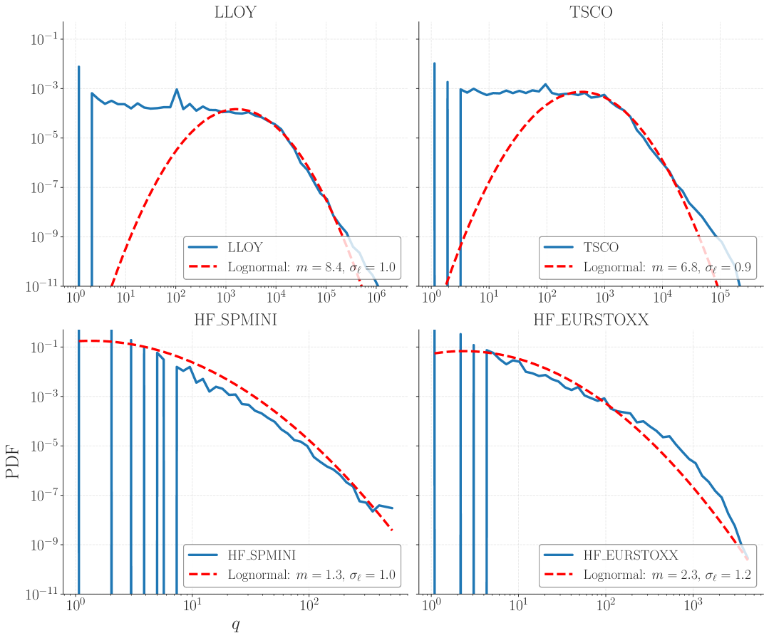
Figure 1: Comparison between the empirical probability distribution functions of the executed volume $q$ for the four selected assets, along with a fitted lognormal distribution in the tail region.

3.4.2 Distribution of sign imbalances

We show in Fig. 2 the distribution of rescaled sign imbalances $I^{0}T^{-\chi}$, for different $T$ in trade time and $\chi=0.72$. The theoretical analysis performed in the previous sections predicts that such distributions should collapse when $\chi$ is chosen to be $1/\mu$, where $\mu=1+\gamma$ is related to the autocorrelation of the sign of the trades, which gives $\mu\approx 1.4$. Although not perfect, the agreement is quite reasonable, in view of the fact that $\mu$ actually depends on the size of the child order $q$, see Fig. 3. The master curve is clearly non-Gaussian, with tails that become fatter as $T$ increases, as expected from our theoretical prediction.

Figure 2: Distribution of sign imbalances $I^{0}$ as a function of the window size $T$ (measured in number of trades) on EUROSTOXX, between 2016 and 2019. After a proper rescaling by $T^{-\chi}$, with $\chi=0.72$, distributions nicely collapse onto a single master curve, consistent with findings in [42]. The value of $\chi$ is not far from the theoretical prediction $\chi=1/\mu$ with $\mu=3/2$. The dotted line shows a Gaussian distribution with the same variance as red curve. As expected, the volume imbalance exhibits fat tails.

3.4.3 Sign autocorrelation function for different child volumes

Intuitively, the sign of large child orders should have shorter memory than small ones. Traders who have large quantities $Q$ to execute is likely to trade small lots in order not to reveal information, whereas smaller $Q$ might be possible to execute in a few shots.

In order to test this hypotheses, we define five logarithmic bins for the rescaled volume $\tilde{q}=q/\phi_{D}$ where $\phi_{D}$ is the daily traded volume. We then compute for each bin the autocorrelation function $C_{\mathcal{B}(\tilde{q})}(\tau)=\operatorname{\mathbb{E}}[\varepsilon_{{B}(\tilde{q})}(t)\varepsilon_{{B}(\tilde{q})}(t+\tau)]$. We removed the largest bin, as it contains outliers, and present the four other autocorrelation functions in Fig. 3, in log-log, together with the unconditional autocorrelation function. As expected, the effective memory exponent $\gamma$ increases with $q$, going from $0.6$ to $1.3$. We take this observation as a qualitative justification of the specification proposed above, i.e. that $\mu_{q}=1+\gamma_{q}=\mu_{1}+\lambda\log q$, which as we now show, allows us to make quantitative predictions for the scaling of the generalized volume imbalances $I^{a}(T)$.

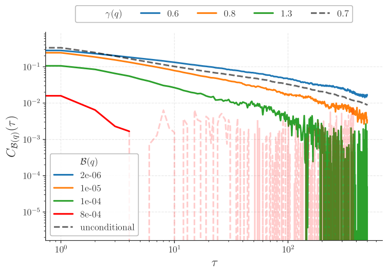
Figure 3: Evolution of the sign autocorrelation of market orders based on their corresponding volume bin $\mathcal{B}(q)$. We used data from the EUROSTOXX, between 2016 and 2019 rescaling market order volume $q$ by the daily traded volume. Our findings indicate that larger market orders tend to be less correlated than smaller ones. Note that nearly $4\%$ of market orders fall into the largest bin.

3.4.4 Scaling of the generalized volume imbalances

Our model predicts that the even moments $\Sigma_{a}^{(2n)}$ of the generalized volume imbalances $I^{a}$ scale with $T$ with exponents that depend on $a$, see Eq. (34). In order to test this prediction empirically, we first remark that trade-by-trade data typically exhibit numerous outliers (such as block trades, fat fingers etc…). These outliers can substantially influence the empirical estimation of the diffusion coefficient, particularly for large values of $a$. Consequently, trades quantities were clipped beyond 1% of the daily volume.

The moments $\Sigma_{a}^{(2n)}$ for $n=1,2,3$ are shown in Fig. 4 as a function of $a$. Remarkably, the theoretical predictions qualitatively reproduce the empirical data, in spite of the rather uncontrolled approximations made in the calculations. In particular, we do find that for large enough $a$, all these moments scale proportionally to $T$, whereas super-linear behaviour in $T$ is observed for small $a$, as a consequence of the long memory of order signs. Such behaviour is washed away when we look at large volumes only, i.e. when $a$ is large enough.

Looking in particular at the curves for $n=1$, we see that $\widetilde{\mu}(a)$ decreases from $\widetilde{\mu}(a=0)\approx 3/2$ to $\widetilde{\mu}(a=a_{c})\approx 2$ with $a_{c}\approx 1$ for large tick EUROSTOXX and $a_{c}\approx 2$ for smaller tick LLOY, TSCO and SPMINI. From Eq. (31), we deduce that $\lambda\sigma_{\ell}^{2}\approx 1/4$ for EUROSTOXX, and $\lambda\sigma_{\ell}^{2}\approx 1/8$ for LLOY, TSCO and SPMINI.

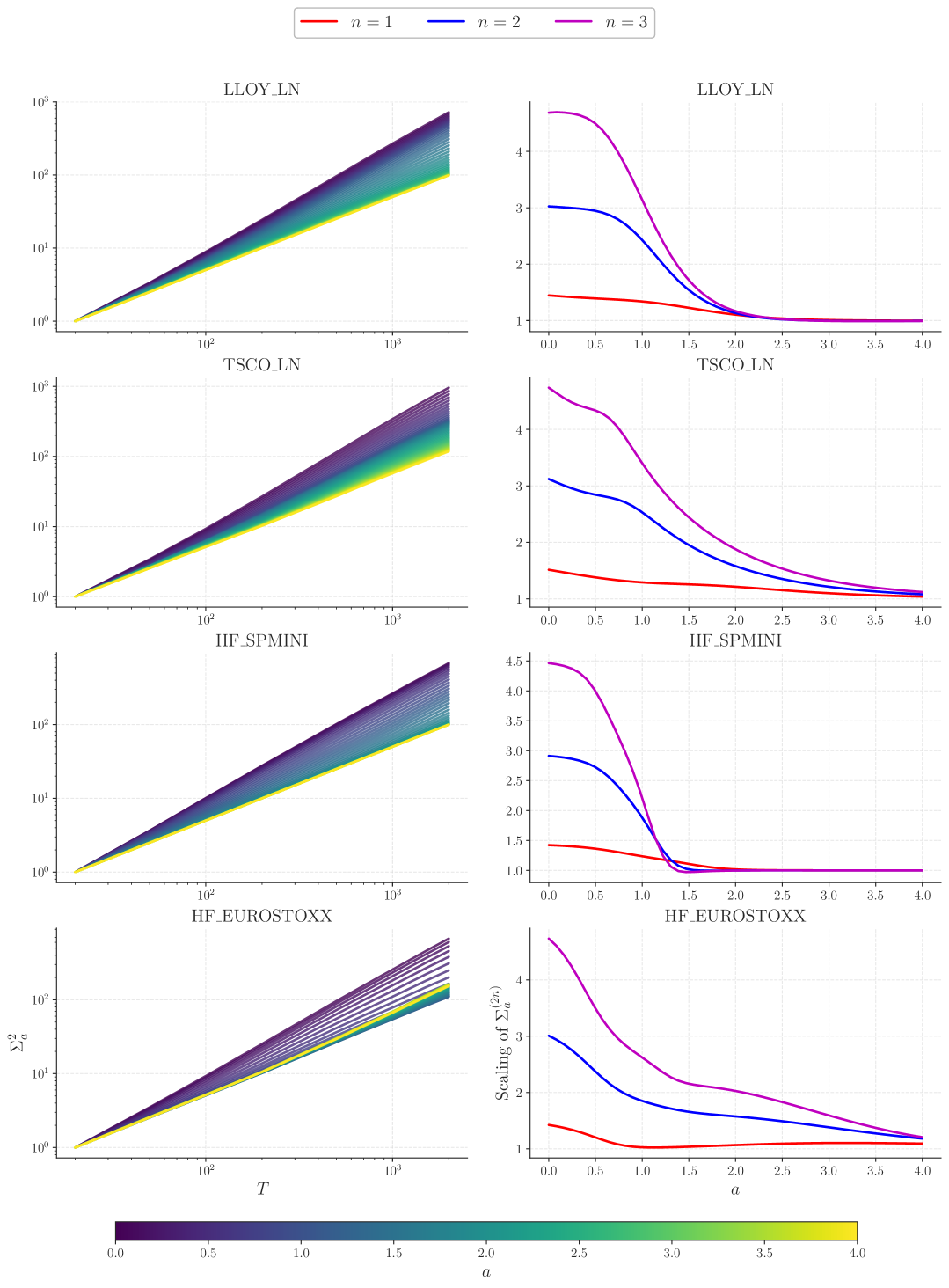
Figure 4: Data for LLOY, TSCO, SPMINI and EUROSTOXX. Right column: scaling of the different moments $\Sigma_{a}^{(2n)}$ as a function of trade time $T$, from which we extract the exponent from a regression of the data in log-log. Left column: scaling exponent as a function of $a$. As predicted by our model, increasing the value of $a$ – i.e. giving more weight to orders with large volume – reduces the value of the exponent, which reaches unity for $a>a_{c}(n)$ with $a_{c}(1)\approx 2$ for LLOY, TSCO and SPMINI, and $a_{c}(1)\approx 1$ for EUROSTOXX.

4 The Impact-Diffusivity puzzle and a generalized propagator

We now discuss the problem of whether the volatility of price changes can be explained chiefly in terms of the impact of intertwined metaorders of different sizes and signs that get executed in the market, i.e. without a “Fundamental” component that makes prices move without any trades. We will first recall how price diffusivity and long-memory of order flow are reconciled within the standard “propagator” framework, and then show how the issue becomes much more perplexing when the impact of metaorders obeys the square-root law. Three possible resolutions are proposed, together with their strengths and weaknesses.

4.1 Price diffusivity within the propagator model

We first assume the impact of single orders is given by a deterministic propagator model, i.e. the average price change due to an order of volume $q$ executed at time $t=0$ is $\theta(q)$ which then decays as [17, 2]

$$G(t)=\theta(q)\,\left(\frac{\tau_{0}}{t+\tau_{0}}\right)^{\beta},$$ (41)

where $\tau_{0}$ is the average time between two child orders. The average impact of a single metaorder of volume $Q$, duration $s\gg\tau_{0}$ and chosen participation rate $\widetilde{\varphi}$ (such that $Q=q\widetilde{\varphi}s$) is then given by

$$\mathcal{I}(t\leq s)=\theta(q)\int_{0}^{t}{\rm d}t^{\prime}\,\widetilde{\varphi}\left(\frac{\tau_{0}}{t-t^{\prime}}\right)^{\beta}=\mathcal{I}_{0}(q,\widetilde{\varphi})t^{1-\beta},\qquad\mathcal{I}_{0}(q,\widetilde{\varphi}):=\frac{\widetilde{\varphi}\theta(q)\tau_{0}^{\beta}}{1-\beta}.$$ (42)

The peak impact $\mathcal{I}(s)$ reads

$$\mathcal{I}(s)=\frac{\widetilde{\varphi}\theta(q)s^{1-\beta}\tau_{0}^{\beta}}{1-\beta}=\frac{\theta(q)q^{\beta-1}(\widetilde{\varphi}\tau_{0})^{\beta}}{1-\beta}Q^{1-\beta},$$ (43)

which reveals one problematic flaw of the propagator model: for $\beta=1/2$, peak impact does not only depend on $Q$, as empirically observed, but also on $q$ and $\widetilde{\varphi}$. Although one can always choose $\theta(q)\propto q^{1-\beta}$ to get rid of the $q$ dependence, one is still left with a square-root dependence on the participation rate $\widetilde{\varphi}$.

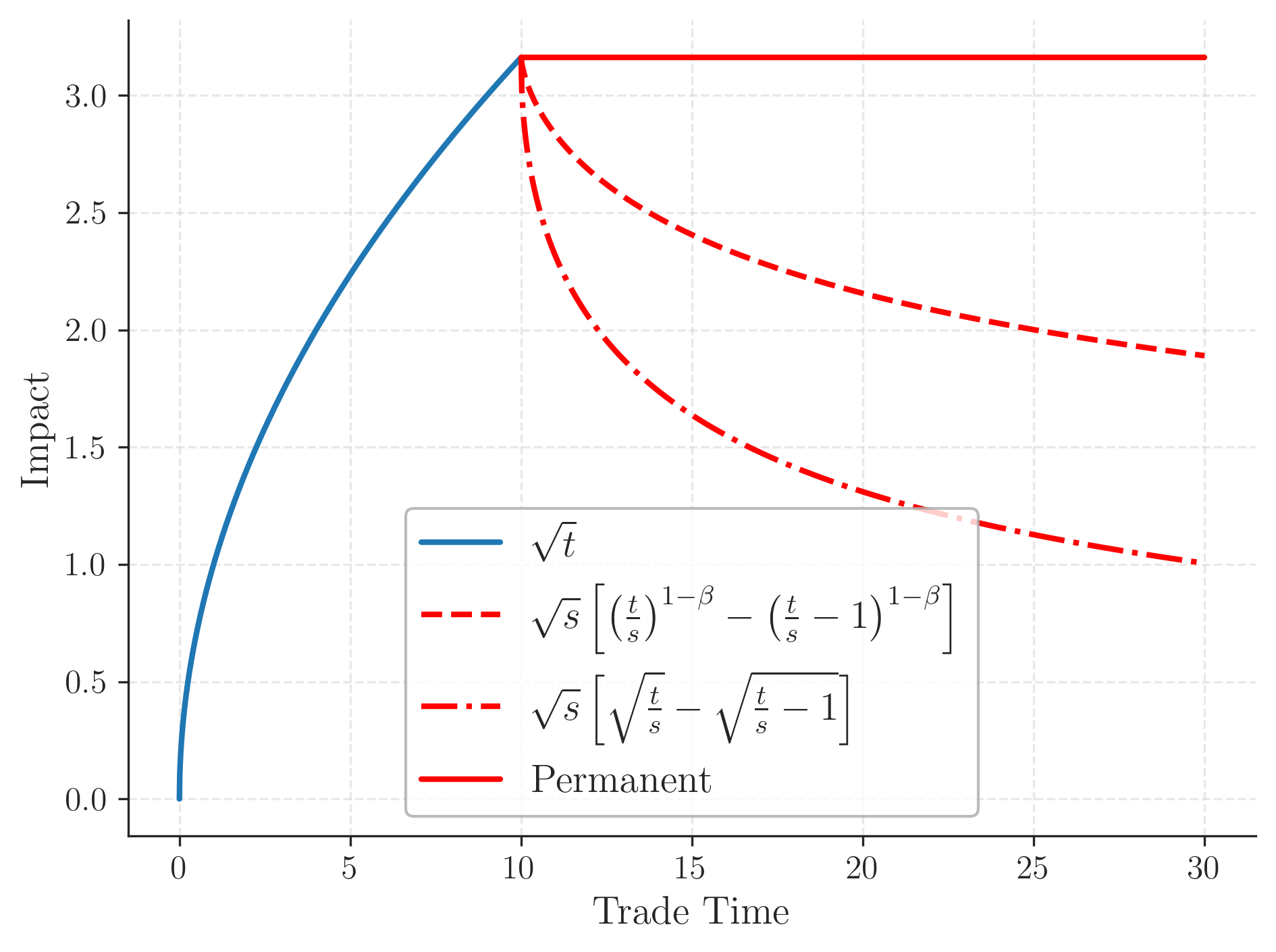
Figure 5: Comparison of the three main theories of impact decay for a metaorder of size $s=10$. During the execution phase (blue), impact follows a square-root impact growth, i.e. $\propto\sqrt{t}$, where $t$ denotes the index of the child order [31, 35]. In the post-execution phase (red), impact may either remain permanent (solid line) or decay (dashed). Two distinct decay mechanisms are illustrated: one based on the generalized two-time propagator as $t^{-\beta}$ with $\beta=0.2$, and the other on the LLOB theory, corresponding to $\beta=\frac{1}{2}$.

After the end of the metaorder, impact decays (see Fig. 5) and is given by

$$\mathcal{I}(t>s)=\theta(q)\int_{0}^{s}{\rm d}t^{\prime}\,\widetilde{\varphi}\left(\frac{\tau_{0}}{t-t^{\prime}}\right)^{\beta}=\mathcal{I}_{0}(q,\widetilde{\varphi})\left(t^{1-\beta}-(t-s)^{1-\beta}\right).$$ (44)

Note that this last expression behaves as $\mathcal{I}(s)(s/t)^{\beta}$ for $t\gg s$.

For simplicity, we assume for now that all market orders have the same volume $q$, and model the price variation $\Delta_{T}$ over time $T$ as the superposition of the average impact of metaorders, neglecting fluctuations that will be considered in section 4.5 below.

Neglecting any “Fundamental” contributions, price variations are then given by the sum of two terms, $\Delta_{T,1}$ describing the impact of metaorders initiated within $[0,T]$, and $\Delta_{T,2}$ the decaying impact of metaorders initiated before $t=0$:

$$\Delta_{T,1}=\mathcal{I}_{0}(q,\varphi)\int_{0}^{T}{\rm d}N_{t}\,\varepsilon(t)\left[\mathbb{I}(t+s>T)(T-t)^{1-\beta}+\mathbb{I}(t+s<T)\left((T-t)^{1-\beta}-(T-t-s)^{1-\beta}\right)\right]$$ (45)

and

$$\Delta_{T,2} =\mathcal{I}_{0}(q,\varphi)\int_{-\infty}^{0}{\rm d}N_{t}\,\varepsilon(t)\left[\mathbb{I}(t+s>T)\left((T-t)^{1-\beta}-(-t)^{1-\beta}\right)\right.$$

$$\hskip 113.81102pt\left.+\mathbb{I}(t+s<T)\left((T-t)^{1-\beta}-(T-t-s)^{1-\beta}-(-t)^{1-\beta}\right)\right]$$ (46)

The average of $\Delta_{T}$ over $\varepsilon$ is of course nil, and its variance is given by two contributions :

$$\Sigma^{2}_{T,1}=\mathcal{I}_{0}^{2}(q,\varphi)\nu\int_{0}^{T}{\rm d}u\,\int_{0}^{\infty}{\rm d}s\,\Psi(s)\left[\mathbb{I}(s>u)u^{2(1-\beta)}+\mathbb{I}(s<u)\left(u^{1-\beta}-(u-s)^{1-\beta}\right)^{2}\right]$$ (47)

and

$$\Sigma^{2}_{T,2} =\mathcal{I}_{0}^{2}(q,\varphi)\nu\int_{T}^{\infty}{\rm d}u\,\int_{0}^{\infty}{\rm d}s\,\Psi(s)\left[\mathbb{I}(s>u)\left(u^{1-\beta}-(u-T)^{1-\beta}\right)^{2}\right.$$

$$\hskip 113.81102pt\left.+\mathbb{I}(s<u)\left(u^{1-\beta}-(u-s)^{1-\beta}-(u-T)^{1-\beta}\right)^{2}\right]$$ (48)

All these contributions can be exactly computed for large $T$ when $\Psi(s)$ decays as a power-law $s^{-(1+\mu)}$, but provided $\mu<2$ the scaling can simply be obtained by the change of variables $s=xT$, $u=yT$, that yields

$$\Sigma_{T}^{2}:=\mathbb{E}[\Delta_{T}^{2}]\propto\mathcal{I}_{0}^{2}(q,\varphi)\,T^{3-2\beta-\mu}.$$ (49)

Hence, we see that metaorders contribute to volatility provided $3-2\beta-\mu=1$. This equality coincides, as expected, with the critical condition $2\beta=1-\gamma$ derived within the propagator model (recall that $\gamma=\mu-1$). When $\beta<(1-\gamma)/2$, the price is super-diffusive (i.e. $\gg T$), whereas when $\beta>(1-\gamma)/2$, the contribution of the average impact of metaorders to price variance is negligible, i.e. $o(T)$.

In order to recover the square-root impact law, one should naively set $\beta=1/2$, such that $3-2\beta-\mu=1-\gamma$. But the contribution of metaorders to volatility $\Sigma_{T}^{2}$ would be then subdominant at long times, unless $\gamma\to 0$ (i.e. an hyper-slow decay of the sign autocorrelation function). Note that the choice $\beta=1/2^{-},\gamma=0^{+}$ corresponds to the model advocated by Jusselin & Rosenbaum [43], but is difficult to reconcile with the empirically determined value $\gamma\approx 0.5$ [37]. This value of $\gamma$, in turn, means that a square-root impact appears to be unable to generate price diffusion, since in this case $3-2\beta-\mu\approx 0.5<1$.

One could then argue that volatility does not primarily come from the average impact of metaorders, but rather from its fluctuations, a possibility that we explore in section 4.4 below. But in any case, the propagator model with $\beta=1/2$ fails to account for two important stylized facts:

• Injecting $\beta=1/2$ into Eq. (42), one finds, as already mentioned above, $\mathcal{I}(s)\propto\sqrt{\widetilde{\varphi}\tau_{0}}\,\sqrt{Q}$ when $\theta(q)=\sqrt{q}$ (as indeed suggested by the data of [35]). Hence, one recovers the square-root law $\mathcal{I}(Q)=Y\sqrt{Q}$ but with an extra square-root dependence of the prefactor $Y$ on the participation rate $\widetilde{\varphi}$, when empirical data show that $Y$ is all but independent of $\widetilde{\varphi}$.

• The decay of impact after the end of a metaorder, when fitted with Eq. (44), suggests a value $\beta\approx 0.2<1/2$ [22, 25, 35], i.e. a much faster short time decay and a much slower long time decay than predicted by $\beta=1/2$.

We conclude that the propagator model, even with $\beta=1/2$ cannot fully explain the observed impact of metaorders, nor its post-execution decay. In the following sections, we explore different routes to reconcile metaorder impact with long-term volatility.

4.2 A generalized propagator model

As we just discussed, the square-root price profile during the execution of the metaorder and the subsequent impact decay cannot be captured within the standard propagator model. Here we propose a (somewhat ad-hoc) extension of this model that allows one to decouple these two profiles. We will not attempt to fully justify such a proposal from first principles, but use the resulting equations as a convenient way to capture the known phenomenology of metaorder impact.

Let us assume that once a metaorder has started, the market slowly adapts and, in the spirit of the LLOB model [33, 2], progressively provides more liquidity to absorb the incoming flow. We represent this effect as a two-time propagator, describing the impact of a child order occurring at time $t^{\prime}$ after the start of the metaorder on the price at time $t>t^{\prime}$:

$$G(t^{\prime}\to t)=\frac{\theta(q)}{(\widetilde{\varphi}t^{\prime}+n_{0})^{1/2-\beta}}\left(\frac{\tau_{0}}{t-t^{\prime}+\tau_{0}}\right)^{\beta},\qquad(\beta<\frac{1}{2})$$ (50)

where $\tau_{0}$ is the average time between two trades and $\widetilde{\varphi}\times t^{\prime}$ is number of child orders executed since the start of the metaorder, which have eaten into the LLOB and therefore reveal more hidden liquidity. $n_{0}$ is the number of trades after which the metaorder is statistically detected by liquidity providers. The immediate impact of a child order is thus

$$G(t^{\prime}\to t^{\prime})=\frac{\theta(q)}{(\widetilde{\varphi}t^{\prime}+n_{0})^{1/2-\beta}}$$ (51)

which decreases with $t^{\prime}$, as liquidity adapts.

The impact of a metaorder of duration $s\gg\tau_{0}$ and $\widetilde{\varphi}s\gg n_{0}$ is now given by

$$\mathcal{I}(t\leq s)\approx\theta(q)\int_{0}^{t}{\rm d}t^{\prime}\,\frac{\widetilde{\varphi}^{1/2+\beta}}{t^{\prime 1/2-\beta}}\left(\frac{\tau_{0}}{t-t^{\prime}}\right)^{\beta}=\mathcal{I}_{1}(q,\widetilde{\varphi})\sqrt{t},\quad\mathcal{I}_{1}(q,\widetilde{\varphi}):=\mathcal{B}_{\beta}\,\sqrt{\widetilde{\varphi}}\theta(q)(\widetilde{\varphi}\tau_{0})^{\beta},$$ (52)

where $\mathcal{B}_{\beta}=2\Gamma(1/2+\beta)\Gamma(1-\beta)/\sqrt{\pi}$.

After the end of the metaorder, impact now decays as

$$\mathcal{I}(t>s)=\mathcal{I}_{1}(q)\sqrt{s}\left[\left(\frac{t}{s}\right)^{1-\beta}-\left(\frac{t}{s}-1\right)^{1-\beta}\right],$$ (53)

which reproduces the empirical decay of metaorders if one chooses $\beta\approx 0.2$. With $\theta(q)\propto\sqrt{q}$, the peak impact then reads

$$\mathcal{I}(Q)\propto(\widetilde{\varphi}\tau_{0})^{\beta}\sqrt{Q},$$ (54)

which still depends on the participation rate, but now with a smaller exponent $\beta=0.2$, more difficult to exclude empirically.

One could have hoped that the slower relaxation of impact in the post-execution regime would help recover a linear-in-$T$ behaviour of $\Sigma_{T}^{2}:=\mathbb{E}[\Delta_{T}^{2}]$. Unfortunately, one finds that the contribution of metaorder impact to $\Sigma_{T}^{2}$ scales as

$$\Sigma_{T}^{2}\propto_{T\to\infty}\begin{cases}T^{1-\gamma},&\quad\gamma<2\beta;\\ T^{1-2\beta},&\quad\gamma>2\beta,\end{cases}$$ (55)

which is again sub-diffusive whenever $\beta>0$ and $\gamma=\mu-1>0$. In other words, impact-driven price diffusion is only possible when impact is permanent, i.e. $\beta=0$. This is in fact the assumption made by Sato & Kanasawa in their latest paper [45]. However, all empirical data known to us suggest that impact decays, at least over short to medium time scales [31, brokmann2015slow, 25, 28], which according to our calculation should lead to substantial price mean reversion on such time scales.

We now turn to three possible resolutions of the diffusion “paradox”: one based on the autocorrelation of the sign of metaorders, a second one based on the permanent impact of large child orders, and the last one based on permanent impact fluctuations.

4.3 The role of metaorder autocorrelations

What happens if we assume, as in section 3.3, that metaorders themselves are autocorrelated, with a new exponent $\gamma_{\times}$? Extending the calculation of $\mathbb{E}[\Delta_{T}^{2}]$ the case $\gamma>\beta-1/2$ (always satisfied when $\beta<\frac{1}{2}$), we find that these correlations contribute to volatility as

$$\mathbb{E}[\Delta_{T}^{2}]_{o.d.}\propto\Gamma\,T^{2-\gamma_{\times}-2\beta}.$$ (56)

This leads to diffusion provided $\gamma_{\times}=1-2\beta$, which is, not surprisingly, the same condition as for the standard propagator model but with $\gamma$ replaced by $\gamma_{\times}$. Indeed, after coarse graining metaorders into effective single orders, we are back to the usual propagator model.

For $\beta=0.2$, this gives $\gamma_{\times}=0.6$, which is close to $\gamma$ itself and close to its empirical value [23] and G. Maitrier (unpublished). It is also compatible with the bound obtained in Eq. (38), which ensures that the autocorrelation of signs is dominated by the size distribution of metaorders, as postulated by [38] and firmly established in [37].

The resulting value of volatility $\sigma^{2}$, defined as $\Sigma_{T}^{2}/T$, is given by

$$\sigma^{2}=C(\beta,\gamma_{\times})\Gamma\nu^{2}\tau_{0}^{\gamma_{\times}}\mathcal{I}_{1}^{2}(q,\varphi)\left(\overline{s^{\frac{1}{2}+\beta}}\right)^{2}+\sigma^{2}_{F},$$ (57)

where $C(\beta,\gamma_{\times})$ is a numerical coefficient found to be $\approx 5.6$ for $\gamma_{\times}=0.6$ and $\beta=0.2$, and $\sigma_{F}$ is the possible “Fundamental” component of volatility (i.e. news driven).

With $\theta(q)=\theta_{0}\sqrt{q}$ and $\phi=\nu q\varphi\bar{s}$, we finally find

$$\theta_{0}=Y\frac{\sigma}{\sqrt{\phi}},\qquad Y\propto\frac{\bar{n}^{\frac{1}{2}-\beta}}{\sqrt{C\Gamma}}\times\sqrt{1-\frac{\sigma_{F}^{2}}{\sigma^{2}}}$$ (58)

where we have assumed that $(\overline{s^{\frac{1}{2}+\beta}})^{2}\propto\bar{s}^{1+2\beta}$, which is justified in the present case since the $(1/2+\beta)$-th moment of $s$ converges (whenever $\mu=1+\gamma>\frac{1}{2}+\beta$). We recall that $\bar{n}=\varphi\bar{s}$ is the average number of child orders per metaorder.

This result is interesting since the peak impact is then precisely given by the standard square-root law, up to a weak participation rate dependence:

$$\mathcal{I}(Q)\propto\left({\widetilde{\varphi}\tau_{0}}\right)^{\beta}\sigma\sqrt{\frac{Q}{\phi}}.$$ (59)

Note that we find naturally that impact is proportional to volatility, simply because volatility is due to impact!

The above calculation can be generalized to higher moments of $\Delta_{T}$. Assuming Wick-like factorisation of $\mathbb{E}[\varepsilon(t_{1})\cdots\varepsilon(t_{2n})]$ as

$$\mathbb{E}[\varepsilon(t_{1})\cdots\varepsilon(t_{2n})]\propto\underbrace{\prod_{i\neq j}|t_{i}-t_{j}|^{-\gamma_{\times}}}_{\text{$n$ pairs}},$$ (60)

it is easy to show that the $2n$-th moment of $\Delta_{T}$ scales as:

$$\Sigma_{T}^{(2n)}\propto T^{2n(1-\beta)-n\gamma_{\times}}=T^{n},$$ (61)

as indeed observed empirically (up to subleading corrections that can also be rationalized within our framework), see Fig. 6.

Note that we do not observe mutifractality (i.e. $\Sigma_{T}^{(2n)}\propto T^{\zeta_{n}}$ with $\zeta_{n}\neq n$) because we work in trade time and not in real time. As it is well known, multifractal effects come from intermittent fluctuations of the activity rate $\nu$, see e.g. [46, 43]. An interesting extension of our model, which we leave for future work, would be to assume that $\nu$ itself has fractal properties.

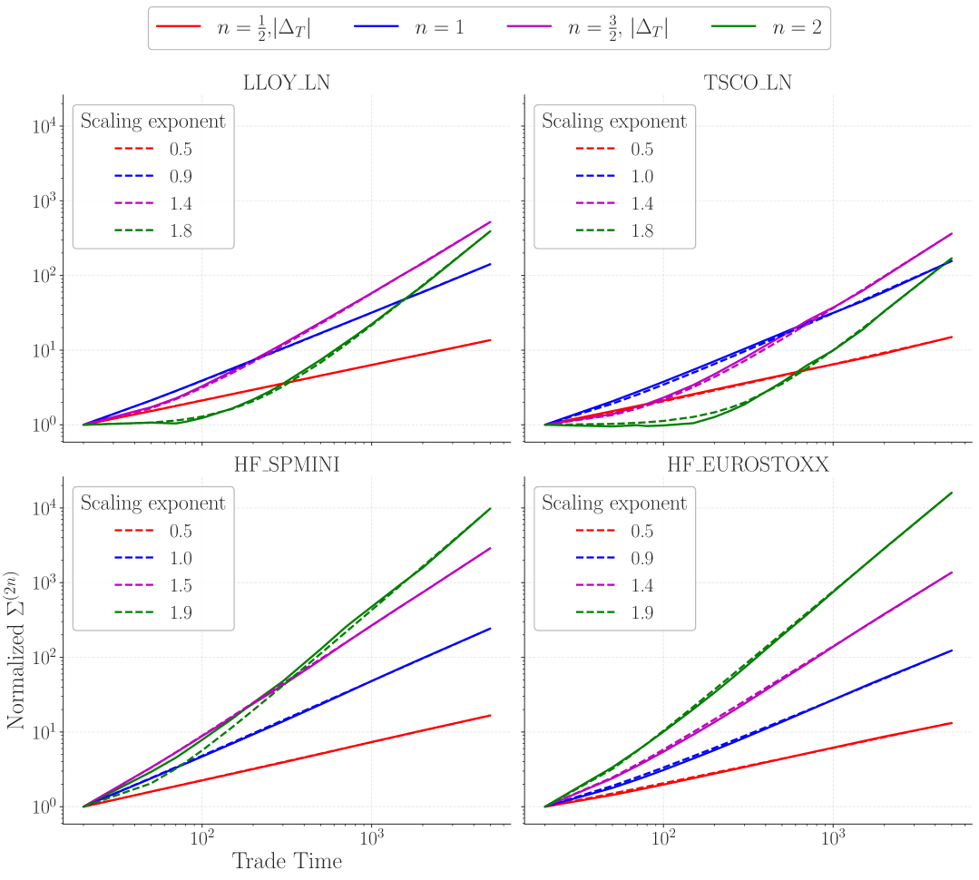
Figure 6: Scaling of the moments of price changes $|\Delta_{T}|^{2n}$ as a function of trade time $T$. We normalized the moment values such that all curves begin at $1$ for $T=1$. As shown, a sublinear behavior is found at short times for $n>1$, likely attributable to price jumps that may dominate for short time scales when $n$ increases. Therefore, we fitted the data as $\Sigma^{(2n)}=a_{0}+a_{1}T^{\zeta_{n}}$ and present the values of $\zeta_{n}$ in the legend. We find in all cases $\zeta_{n}\approx n$, up to subleading corrections that we attribute to volume fluctuations.

4.4 The role of volume fluctuations

Another possibility is to take seriously the fact that the size $q$ of child orders is fluctuating and correlated with the duration $s$ of metaorders. As we have shown in section 3.2, a dependence of the exponent $\mu_{q}$ on $q$ explains how different moments of the volume imbalance depend on $T$, see Eqs. (32), (34). It is also in agreement with direct empirical results, see Fig. 3.

Now, similarly to $\mu_{q}$, we might assume that the impact decay exponent $\beta$ becomes $q$-dependent: $\beta_{q}=\beta_{1}-\lambda^{\prime}\log q$. One then observes that price impact becomes permanent for large child orders, with $q>q_{0}$ such that $\beta_{q}\leq 0$. When metaorder signs are independent, the non-vanishing contribution to volatility then reads:

$$\mathbb{E}[\Delta_{T}^{2}]_{q>q_{0}}=\nu\int_{q_{0}}^{\infty}{\rm d}q\,\Xi(q)\mathcal{I}_{1}^{2}(q,\varphi)\int_{0}^{T}{\rm d}u\,\int_{0}^{u}{\rm d}s\,\Psi_{q}(s)s\approx_{T\to\infty}\nu T\int_{q_{0}}^{\infty}{\rm d}q\,\Xi(q)\mathcal{I}_{1}^{2}(q,\varphi)\bar{s}_{q}.$$ (62)

Taking $\theta(q)=\theta_{0}\sqrt{q}$ one gets $\mathcal{I}_{1}(q>q_{0},\varphi)=2\theta_{0}\sqrt{\varphi q}$, so the contribution to long-term price volatility is given by

$$\sigma^{2}=\frac{\mathbb{E}[\Delta_{T}^{2}]_{q>q_{0}}}{T}\propto\theta_{0}^{2}\phi_{0},$$ (63)

where $\phi_{0}$ is the average volume flow of the market, restricted to “large” child orders $q>q_{0}$. Interestingly, this relation can be read backwards as

$$\theta_{0}\propto\frac{\sigma}{\sqrt{\phi_{0}}},$$ (64)

allowing one to recover the full square-root impact law from the expression of $\mathcal{I}_{1}$ above:

$$\mathcal{I}(Q|q,\widetilde{\varphi})=Y(q,\widetilde{\varphi})\sigma\sqrt{\frac{Q}{\phi}},\qquad Y(q,\widetilde{\varphi})\propto(\widetilde{\varphi}\tau_{0})^{\beta_{q}}\,\sqrt{\frac{\phi}{\phi_{0}}}.$$ (65)

We see that this result suggests a weak dependence of the prefactor of the square-root law in $q$ and $\widetilde{\varphi}$, which disappears for large enough $q>q_{0}$, since $\beta_{q}\to 0$ in that case. However, in that case $Y$ would be substantially larger than empirically observed, since from Fig. 3 we estimate $\phi_{0}\approx 0.1\phi$. Besides, since child orders of size $<q_{0}$ (which are the most numerous) only impact prices temporarily, this scenario would again lead to strong visible mean-reversion in prices not observed in data – see e.g. Fig. 6 for $n=1$.

It is, however, important to discuss how volume fluctuations might affect the result Eqs. (55), (56) above, induced by the correlation between different metaorders. It is plain to extend the calculations of section 3.3 to get

$$\mathbb{E}[\Delta_{T}^{2}]_{o.d.}\propto\Gamma e^{m+\frac{\sigma_{\ell}^{2}}{4}}\,T^{2-\gamma_{\times}-2\beta_{m}+\lambda^{\prime}\sigma_{\ell}^{2}},$$ (66)

whereas a similar calculation for the diagonal contribution gives

$$\mathbb{E}[\Delta_{T}^{2}]_{d.}\propto e^{m+\frac{\sigma_{\ell}^{2}}{2}}\,T^{1-2\beta_{m}+2\lambda^{\prime}\sigma_{\ell}^{2}}.$$ (67)

The ratio of the prefactors is now only $e^{\sigma_{\ell}^{2}/4}/\Gamma$ in favor of the diagonal term. This means that the off-diagonal contribution, with a larger power of $T$, becomes dominant beyond a reasonable small value of $T$ when $\sigma^{2}_{\ell}=1$ and $\Gamma=O(1)$. We will therefore choose in the following $\gamma_{\times}=0.6$ and $\widehat{\beta}(0):=\beta_{m}-\frac{1}{2}\lambda^{\prime}\sigma_{\ell}^{2}=0.2$, such that the off-diagonal contribution is exactly diffusive.

4.5 The role of impact fluctuations

Up to now, we have assumed deterministic impact and neglected the role of price changes induced by “news” or other order book events that are not related to trades, with the ambition of recovering all the price volatility from the impact of metaorders. However, it is clear that:

• (i) news events do obviously exist (see e.g. [47] for a recent discussion) and should indeed contribute to volatility. In fact, Efficient Market Theory predicts that the only contribution to volatility comes from news!

• (ii) the impact of a given metaorder has no reason to be deterministic: it should depend on specific time-dependent market conditions and thus include a random component.

Such a random component was in fact indirectly observed by Bucci et al. [30], where it was found that the effect of a single metaorder on price changes reads

$$\Delta_{T}=p_{T}-p_{0}\approx\varepsilon\mathcal{I}(Q)\left[1+z\eta\right],$$ (68)

where $\eta$ is a zero mean, unit variance, independent random variable, and $z$ a coefficient measuring the relative fluctuations of impact, found to be around $3$ in [30].

Let us postulate that, while the average impact decays to zero with time as per the propagator model, the random component $z\eta$ does not, or at least not completely. This assumption does not violate any known stylized facts about the average decay of impact. Following these ideas, we expect price changes $\Delta_{T}$ to include extra terms that read

$$\Delta_{T,1}=z_{\infty}\theta_{0}\sqrt{q\varphi}\int_{0}^{T}{\rm d}N_{t}\,\varepsilon(t)\left[\mathbb{I}(t+s>T)\sqrt{T-t}+\mathbb{I}(t+s<T)\sqrt{s}\right]\eta_{t}+\sigma_{F}\xi\sqrt{T},$$ (69)

where $z_{\infty}\leq z$ accounts for a possible time decay of the random component of impact, and the last contribution captures fundamental “news”, with a volatility $\sigma_{F}$. ($\xi$ is another zero mean, unit variance, independent random variable).

This gives rise the following contribution to volatility:

$$\Sigma_{T}^{2}=\mathbb{E}[\Delta_{T}^{2}]_{\eta,\xi}=z_{\infty}^{2}\theta_{0}^{2}q\varphi\nu\int_{0}^{T}{\rm d}u\int_{0}^{\infty}{\rm d}s\Psi(s)\left[\mathbb{I}(s>u)u+\mathbb{I}(s<u){s}\right]+\sigma_{F}^{2}T,$$ (70)

whence a long-term volatility given by

$$\sigma^{2}=\sigma_{F}^{2}+z_{\infty}^{2}\theta_{0}^{2}q\varphi\nu\bar{s}\equiv\sigma_{F}^{2}+z_{\infty}^{2}\theta_{0}^{2}\phi,$$ (71)

where $\phi=q\varphi\nu\bar{s}$ is, again, the average volume flow in the market.

This expression is quite interesting: inserting $\theta_{0}=Y\sigma/\sqrt{\phi}$, we get, provided $Yz_{\infty}<1$:

$$\sigma^{2}=\frac{\sigma_{F}^{2}}{1-Y^{2}z_{\infty}^{2}},$$ (72)

i.e. excess volatility induced by trading, independently of its information content. This is in line with the empirical results of [48] (section 4), [49] and [2] (Figs. 13.2 and 14.5), and is of course related to the well-known excess volatility/excess trading puzzle, see e.g. [14, 13, 15] and [2], chapters 2 & 20, see also [8, 1, 11] for related discussions.

Hence, even if the deterministic, decaying part of impact does not contribute to long-term volatility, its fluctuations might do the job. Of course, this somewhat contorted scenario relies on the assumption that the random component of impact has a permanent contribution to price changes, i.e. $z_{\infty}>0$. Although this hypothesis is somewhat ad-hoc, the non-trivial result here is the relation between price impact and volatility given by

$$\mathcal{I}(Q)\propto\sqrt{\frac{\sigma^{2}-\sigma_{F}^{2}}{z_{\infty}^{2}}}\times\sqrt{\frac{Q}{\phi}}.$$ (73)

If, on the other hand, the permanent contribution $z_{\infty}$ vanishes, then trivially $\sigma^{2}=\sigma_{F}^{2}$. This is the Efficient Market picture, where uninformed trades do not contribute to long-term volatility and our whole construction breaks down. However, this would leave $\theta_{0}$ undetermined and would not allow rationalizing why $\theta_{0}$ is proportional to $\sigma/\sqrt{\phi}$, as found empirically. Furthermore, the impact of uninformed metaorders (which is probably a large fraction of all metaorders) would generate large price reversion effects, which again are not observed.

4.6 Discussion

We thus have three possible scenarios for generating long term volatility from metaorder impact alone. The idea that metaorders are correlated between one another, with roughly the same long memory as within each one of them, seems plausible, is compatible with available data and provides a natural extension of the propagator scenario: diffusive prices emerge from the subtle interplay between decaying impact and autocorrelated order flow. Such a scenario predicts a weak dependence of the prefactor $Y$ of the square-root law with the participation rate of the metaorder, as $\widetilde{\varphi}^{\beta}$ with $\beta\approx 0.2$.

The second scenario, which attributes long term to the non-decaying impact of metaorders executed with large child orders does not seem very credible to us, because it would lead to substantial mean-reversion effects due to the impact decay of small child orders, which is at odds with empirical decay.

Finally, long term volatility may result from the random component of impact, assumed to be permanent. This bypasses the paradox that average impact decays and, in the absence of correlations between metaorders, should lead to subdiffusion. In such a scenario, volatility is induced by trading activity alone, even when average impact is zero. Still, the fact that impact fluctuations are proportional to average impact, as postulated in Eq. (68), is important to recover the correct relation between peak impact $\mathcal{I}(Q)$ and $\sigma\sqrt{Q/\phi}$, Eq. (73), which is now independent of $\widetilde{\varphi}$.

We now turn to the study of the covariance of price changes and volume imbalances, to see whether we can constrain the theory further. In fact, we will see that the data strongly favours an interpretation based on the average impact of long-range correlated metaorders. The last scenario, where volatility arises from the fluctuating part of impact, does not pass the test, as it is unable to reproduce the detailed structure of the correlations between price changes and generalized volume imbalances.

5 Covariance between order flow imbalance and prices changes

An interesting quantity that can be computed within our model and easily measured empirically using the public tape of trades and prices is the “aggregated” impact $\mathbb{E}[\Delta|I^{a}]$, conditioned to a certain value of imbalance $I^{a}$, as studied in [50, 42]. We know that such a quantity behaves very differently from the square-root law, and has non-trivial scaling properties as a function of $T$, see [42] for $a=0$ and $a=1$. For $a=0$, in particular, one finds that the initial slope of $\mathbb{E}[\Delta|I^{0}]$ as a function of $I^{0}$ scales like $T^{-\omega}$ with $\omega\approx 1/4$ [42, 2], a result we confirm in Fig. 7.

Note that if $I^{a}$ and $\Delta$ were Gaussian variables one could use the following general relation to predict that slope:

$$\mathbb{E}[\Delta|I^{a}]=\frac{\mathbb{E}[\Delta\cdot I^{a}]}{\Sigma_{a}^{2}}I^{a},$$ (74)

i.e. a linear aggregate impact for small imbalances, where $\Sigma_{a}^{2}$ was defined in section 3.2. However, in our model the Gaussian assumption does not hold since $I^{a}$ is a truncated Lévy variable (see section 3.2). Hence the exact calculation of $\mathbb{E}[\Delta|I^{a}]$ is much more intricate, and we restrict the following analysis to the covariance $\mathbb{E}[\Delta\cdot I^{a}]$, which we compare to empirical data below. Still, naively applying Eq. (74) will predict a scaling in $T^{-\omega}$, albeit within an uncontrolled approximation.

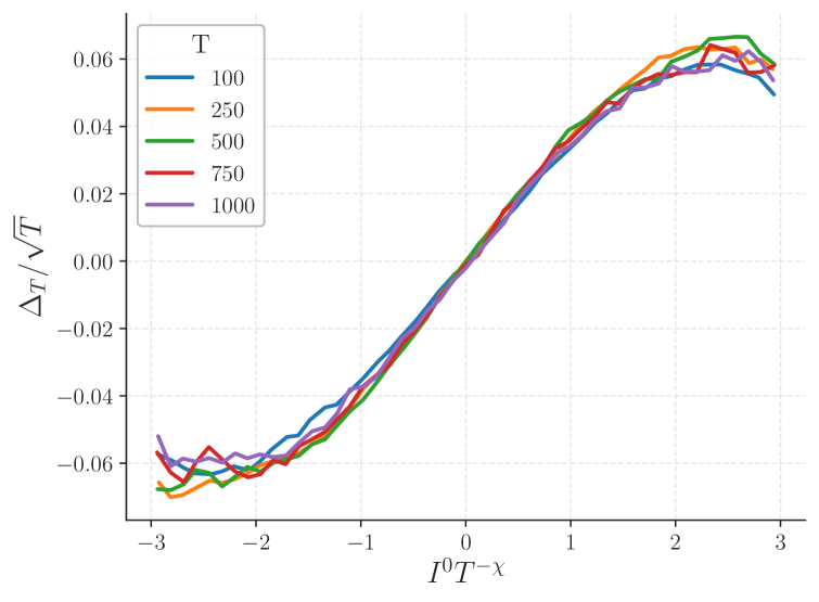
Figure 7: Aggregated impact versus sign imbalance for the EUROSTOXX. After appropriate rescaling, curves for different $T$ nicely collapse onto a single master curve. The y-axis rescaling reflects the diffusive nature of the price, while the x-axis rescaling captures trade sign correlations, as detailed in section 3. In this case, we find $\omega=\chi-\frac{1}{2}\approx 0.22$.

5.1 Without volume fluctuations

Since impact fluctuations, considered in section 4.5, are independent of the order imbalance (i.e. $\mathbb{E}[\varepsilon\eta]=0$), we can restrict the calculation to the deterministic part of impact, which is given by the generalized propagator model above. Neglecting any sign correlations between different metaorders, we thus get, when all child orders have the same size:

$$\mathbb{E}[\Delta_{T}\cdot I_{T}^{a}]=\nu\varphi q^{a}\mathcal{I}_{1}(q,\varphi)\int_{0}^{T}{\rm d}u\int_{0}^{\infty}{\rm d}s\Psi(s)\left[\mathbb{I}(s>u)u\sqrt{u}+\mathbb{I}(s<u)s\sqrt{s}\left((\frac{u}{s})^{1-\beta}-(\frac{u}{s}-1)^{1-\beta}\right)\right].$$ (75)

This quantity scales like $T^{1-\beta}$ whenever $\mu>3/2+\beta$ and like $T^{5/2-\mu}$ otherwise. Note that if one disregards the non-Gaussian nature of $I^{0}$ and uses Eq. (74) to compute the initial slope of the aggregate impact, one finds (using Eq. (17)) $\omega=1/2$ when $\mu=3/2$ and $\beta>0$, which is far from the empirical value $\omega\approx 1/4$. As we shall see in the following, empirical results suggest a strong dependence on $a$, meaning that volume fluctuations certainly cannot be neglected in this calculation.

5.2 With correlated metaorders

One can extend the result above to account for correlated metaorders. Assuming $\gamma>0$ and $\beta<1/2$, the “non-diagonal” contribution $t\neq t^{\prime}$ gives a contribution that scales as

$$\mathbb{E}[\Delta_{T}\cdot I_{T}^{a}]_{o.d.}\propto\Gamma\,q^{a+\frac{1}{2}}\,T^{2-\beta-\gamma_{\times}},$$ (76)

to be compared with the above results, i.e. $T^{1-\beta}$ or $T^{5/2-\mu}$. When $\gamma_{\times}<1$, the non-diagonal contriburion is always dominant at large $T$ compared to $T^{1-\beta}$ and becomes subdominant compared to $T^{5/2-\mu}=T^{3/2-\gamma}$ when $\beta+\gamma_{\times}>1/2+\gamma$.

For $\gamma=\gamma_{\times}$ and $\beta<\frac{1}{2}$ we thus deduce that the “off-diagonal” contribution is always dominant for large enough times. The corresponding value of the slope exponent $\omega$ is now equal to $\beta+\gamma_{\times}-\gamma$, and is thus very close to the empirical value $\omega\approx 1/4$ when $\gamma_{\times}\approx\gamma$ and $\beta\approx 0.2$.

5.3 With correlated metaorders and volume fluctuations

Let us now add volume fluctuations, with a $q$-dependent value of $\mu_{q}$ as given by Eq. (22) and $\beta_{q}=\beta_{1}-\lambda^{\prime}\ell$, with $\ell=\log q$. Now, there exists a value $q=q_{c}^{\prime}$ such that $5/2-\mu_{q_{c}^{\prime}}=1-\beta_{q_{c}^{\prime}}$.

Then, using $\mathcal{I}_{1}(q,\varphi)\propto\sqrt{q}$, one gets, for the diagonal contribution

$$\mathbb{E}_{q}[\Delta_{T}\cdot I_{T}^{a}]_{d.}\propto\int_{0}^{q_{c}^{\prime}}{\rm d}q\,\Xi(q)\,q^{a+\frac{1}{2}}T^{5/2-\mu_{q}}+\int_{q_{c}^{\prime}}^{\infty}{\rm d}q\,\Xi(q)\,q^{a+\frac{1}{2}}T^{1-\beta_{q}},$$ (77)

and for the off-diagonal contribution

$$\mathbb{E}_{q}[\Delta_{T}\cdot I_{T}^{a}]_{o.d.}\propto\Gamma\,\mathbb{E}[q^{a}]\int_{0}^{\infty}{\rm d}q\,\Xi(q)\,q^{\frac{1}{2}}T^{2-\gamma_{\times}-\beta_{q}},$$ (78)

Repeating the same calculations as in section 3.2, we now get:

$$\mathbb{E}_{q}[\Delta_{T}\cdot I_{T}^{a}]_{d.} \propto T^{5/2-\mu_{m}}\int_{0}^{\ell_{c}^{\prime}}{\rm d}\ell\,\,e^{(\ell-m)(a+\frac{1}{2}-\lambda\log T)-(\ell-m)^{2}/2\sigma_{\ell}^{2}}$$

$$+T^{1-\beta_{m}}\int_{\ell_{c}^{\prime}}^{\infty}{\rm d}\ell\,\,e^{(\ell-m)(a+\frac{1}{2}+\lambda^{\prime}\log T)-(\ell-m)^{2}/2\sigma_{\ell}^{2}}.$$ (79)

When $(\lambda,\lambda^{\prime})\log T\ll 1$, the Gaussian integrals are dominated by the region around $\ell^{\star}=m+\sigma_{\ell}^{2}(a+1/2)$. So, schematically, when $\ell^{\star}<\ell_{c}^{\prime}:=\log q_{c}^{\prime}$ the first integral dominates, while for $\ell^{\star}>\ell_{c}^{\prime}$ the second integral dominates. Hence, the dominant term scales as:

$$\mathbb{E}_{q}[\Delta_{T}\cdot I_{T}^{a}]_{d.}\propto e^{m(a+\frac{1}{2})+\frac{1}{2}\sigma_{\ell}^{2}(a+\frac{1}{2})^{2}}\begin{cases}&T^{5/2-\widehat{\mu}(a)},\qquad\widehat{\mu}(a)=\mu_{m}+(a+\frac{1}{2})\lambda\sigma_{\ell}^{2}\qquad\qquad a<a_{c}^{\prime};\\ &T^{1-\widehat{\beta}(a)},\quad\qquad\widehat{\beta}(a)=\beta_{m}-\left(a+\frac{1}{2}\right)\lambda^{\prime}\sigma_{\ell}^{2}\qquad\quad a>a_{c}^{\prime},\end{cases}$$ (80)

where $a_{c}^{\prime}$ is such that $\widehat{\mu}(a_{c}^{\prime})=\mu_{q_{c}^{\prime}}$.

The power of $T$ coming from the diagonal contribution is thus predicted to decrease with $a$ when $a<a_{c}^{\prime}$ and then to increase with $a$ for larger $a$. Hence we expect an interesting non-monotonic behaviour of the effective exponent as a function of $a$, i.e. with the relative weight given to child orders with large volumes.

The off-diagonal contribution, on the other hand, gives:

$$\mathbb{E}_{q}[\Delta_{T}\cdot I_{T}^{a}]_{o.d.}\propto\Gamma\,e^{m(a+\frac{1}{2})+\frac{1}{2}\sigma_{\ell}^{2}(a^{2}+\frac{1}{4})}\,T^{2-\gamma_{\times}-\widehat{\beta}(0)}.$$ (81)

Note that the coefficient in front of the power-law is $\Gamma e^{-\sigma_{\ell}^{2}a/2}$ smaller than the one corresponding to the diagonal contribution. Other numerical prefactors may however contribute as well, that were neglected in the rough estimate of the above integrals. The final theoretical prediction is that $\mathbb{E}_{q}[\Delta_{T}\cdot I_{T}^{a}]$ is the sum of three power-law contributions:

• $T^{5/2-\widehat{\mu}(a)}$, with an exponent equal to $1$ for $a=0$ and decreasing as $a$ increases,

• $T^{1-\widehat{\beta}(a)}$, with an exponent equal to $\approx 0.8$ for $a=0$ and increasing as $a$ increases,

• $T^{2-\gamma_{\times}-\widehat{\beta}(0)}$, with an exponent independent of $a$ and equal to $\approx 1.2$ for the default values of $\gamma_{\times},\widehat{\beta}(0)$.

In section 5.7 below, we will show that empirical data can be fitted as a power-law of $T$, with an effective exponent that indeed behaves non-monotonically with $a$, which suggests $(\lambda,\lambda^{\prime})\sigma_{\ell}^{2}$ in the range $0.1$–$0.2$, also in line with the condition already obtained in section 3.2.

Finally, note that the slope exponent $\omega$, naively predicted from Eq. (74) for $a=0$ is

$$\omega_{d.}=\frac{1}{2}+\widehat{\mu}(0)-\widetilde{\mu}(0)=\frac{1}{2}(1+\lambda\sigma_{\ell}^{2}),\qquad\omega_{o.d.}=1-\widetilde{\mu}(0)+\gamma_{\times}+\widehat{\beta}(0),$$ (82)

depending on whether the diagonal or off-diagonal contribution dominates. Numerically, with $\lambda\sigma_{\ell}^{2}=1/8$ and $\gamma_{\times}+\widehat{\beta}(0)=0.8$, one finds $\omega_{d.}\approx 0.56$ and $\omega_{n.d.}\approx 0.30$, close to the empirical value $1/4$ in the second case.

5.4 With a random impact component

Quite interestingly, if the random component of impact (see Eq. (68)) is assumed to be such that $\mathbb{E}[\varepsilon\eta]=0$, it will not contribute to the covariance between price changes and order imbalance. Indeed, by definition such a contribution to price changes does not contribute to the covariance between price changes and order imbalance. In such a scenario, only the fundamental component can contribute to the covariance, provided some metaorders are “informed”, as we show next.

5.5 With “informed” metaorders

Up to now, we assumed that there are no correlations between the sign of metaorders $\varepsilon$ and the “Fundamental” component of price changes on time scale $T$, $\sigma_{F}\xi\sqrt{T}$, see Eq. (68). If we rather assume that $\mathbb{E}[\varepsilon\xi]=\rho/\sqrt{\nu T}$, where $\rho$ measures the average amount of information of individual metaorders, we find an extra contribution to $\mathbb{E}[\Delta_{T}\cdot I_{T}^{a}]$ computed above, which reads:

$$\mathbb{E}[\Delta_{T}\cdot I_{T}^{a}]=\rho\sqrt{\nu}\varphi q^{a}\sigma_{F}\int_{0}^{T}{\rm d}u\int_{0}^{\infty}{\rm d}s\Psi(s)\left[\mathbb{I}(s>u)u+\mathbb{I}(s<u)s\right].$$ (83)

Extending the calculation above, we now find that this covariance scales as $T^{2-\mu}$ for $\mu<1$ and as $T$ for $\mu>1$, which is the case we focus on here. Note that the naive prediction for the slope exponent $\omega$ (from Eq. (74)) is $\omega=2-\mu$.

Hence, we find that such a fundamental contribution predicts a linear scaling of $\mathbb{E}[\Delta_{T}\cdot I_{T}^{a}]$ as a function of $T$, independently of $a$.

5.6 The correlation coefficient

Finally, we turn our attention with a natural description of the interplay between (generalized) volume imbalance and price changes, namely the following correlation coefficient

$$R_{a}(T):=\frac{\mathbb{E}[\Delta_{T}\cdot I_{T}^{a}]}{\Sigma_{T}\Sigma_{a}},\qquad\Sigma_{T}:=\sqrt{\mathbb{E}[\Delta_{T}^{2}]},\qquad\Sigma_{a}:=\sqrt{\mathbb{E}[I_{T}^{a2}]}$$ (84)

In order to simplify the discussion, we assume that the crossovers between the two regimes for $\Sigma_{a}^{2}$ (Eq. (32)) and for $\mathbb{E}[\Delta_{T}\cdot I_{T}^{a}]$ (Eq. (80)) occur for the same value of $a=a_{c}=a_{c}^{\prime}$. Although this is not precisely true, the following conclusions will be qualitatively correct.

In the case where the sign of metaorders and the fundamental component of price changes are independent ($\rho=0$) and the off-diagonal contribution can be neglected ($\Gamma=0$), we find that for $T\gg 1$:

$$R_{a}(T)_{d.}\propto e^{\frac{\sigma_{\ell}^{2}}{2}a(1-a)}\times\begin{cases}&T^{(1-\mu_{m}-\lambda\sigma_{\ell}^{2})/2},\quad\quad a<a_{c};\\ &T^{-\widehat{\beta}(a)},\qquad\qquad\quad a>a_{c}.\end{cases}$$ (85)

A more refined analysis would be needed for small values of $T$, but from such an analysis we conclude that $R_{a}(T)$ should be decreasing with $T$ for small values of $a$ (since $\mu_{m}\approx 3/2$) and saturating for large values of $a$ (since $\widehat{\beta}(a>a_{c}^{\prime})=0$). Furthermore, note the non-monotonic behaviour (in $a$) of the prefactor in Eq. (85).

If we now consider the contribution coming from the correlation between metaorders, we get:

$$R_{a}(T)_{o.d.}\propto e^{-\frac{\sigma_{\ell}^{2}a^{2}}{2}}\times T^{\mu_{m}/2+a\lambda\sigma_{\ell}^{2}-\gamma_{\times}-\widehat{\beta}(0)}.$$ (86)

For $a\to 0$, the power of $T$ is very close to zero for our default choice of parameters. For higher values of $a$, the exponent becomes positive and therefore this off-diagonal contribution adds an increasing function of $T$.

If we assume instead that $R_{a}(T)$ is dominated by informed metaorders, we obtain, in the regime where $\mu_{q}>1+\beta_{q}$, $\forall q$,

$$R_{a}(T)_{F}\propto\rho e^{-\frac{\sigma_{\ell}^{2}a^{2}}{2}}\times\begin{cases}&T^{\mu_{m}/2+a\lambda\sigma_{\ell}^{2}-1},\quad\quad a<a_{c};\\ &T^{0},\qquad\qquad\,\quad a>a_{c}.\end{cases}$$ (87)

The scaling with $T$ indicates that $R_{a}(T)$ should decrease with $T$ for small values of $a$, and become independent of $T$ for large values of $a$. Note that if volatility is mostly due to fundamentals and not due to impact, one finds that $R_{a}(T)$ is directly proportional to $\rho$.

Hence, we see that the three possible contributions to $R_{a}(T)$ have different monotonicity properties as functions of $T$, suggesting that different shapes of $R_{a}(T)$ might be observed empirically. In the following, we will confirm that this is indeed the case. The behaviour of $R_{a}(T)$ for a given $T$ as a function of $a$ is simpler to describe. One finds that for $a<a_{c}$

$$R_{a}(T)=e^{-\frac{\sigma_{\ell}^{2}a^{2}}{2}}\left(A(T)e^{\frac{\sigma_{\ell}^{2}a}{2}}+B(T)e^{\lambda\sigma_{\ell}^{2}a\log T}\right),$$ (88)

where $A,B$ are functions of $T$, the second contribution $B(T)$ coming from the $a$ dependence of the exponents. Hence we expect a behaviour of $R_{a}(T)$ that always increases for small $a$, independently of the dominant contribution (diagonal, off-diagonal or fundamental), but with a slope that increases with $T$ in the last two cases. These predictions will be tested against empirical data in the next section.

5.7 Empirical data

The theoretical analysis laid out in the previous sections makes several non-trivial predictions:

1. Provided the main source of price moves is the average impact of random metaorders, the covariance $\operatorname{\mathbb{E}}[\Delta_{T}\cdot I_{T}^{a}]$ behaves as a power-law of $T$ with an effective exponent that is non-monotonic in $a$, reaching a minimum for some value of $a$, see Eq. (80). If instead volatility is dominated by the random component of impact (Eq. (68)) with a “Fundamental” component $\sigma_{F}\xi$, a linear behaviour in $T$ independent of $a$ should be observed;

2. The correlation coefficient $R_{a}(T)$ contains an off-diagonal contribution growing with $T$ and two contributions (diagonal and fundamental) decaying with $T$ before saturating. Depending on the relative amplitude of these contributions, different shapes can be expected;

3. For a given $T$, the correlation coefficient $R_{a}(T)$ is predicted to be a humped shape function of $a$.

We will show below that, quite remarkably, all these predictions are in qualitative agreement with empirical data. This will enable us to estimate the parameters $\lambda$ and $\lambda^{\prime}$. We will also see a marked difference between large tick assets like EUROSTOXX and smaller tick assets (LLOY, TSCO and SPMINI).

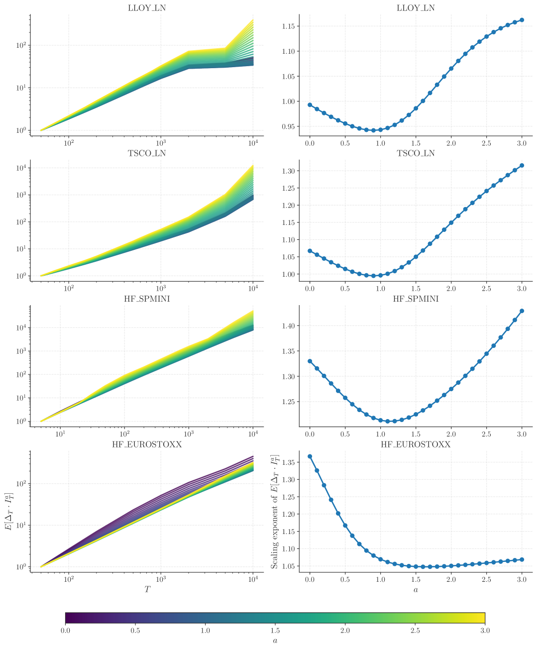
Figure 8: Covariance $(\Delta_{T},I^{a}_{T})$ as a function of $(T,a)$ for the four considered assets. Left: Log-log plot of $\operatorname{\mathbb{E}}[\Delta_{T}\cdot I_{T}^{a}]$ vs. $T$ for different values of $a$. Right: Scaling exponents as a function of $a$, obtained by fitting the initial regime ($T<10^{3}$).

5.7.1 Power-law behaviour of the covariance

We first investigate point 1. above. As shown in Fig. 8 (left), a power-law behaviour of $\operatorname{\mathbb{E}}[\Delta_{T}\cdot I_{T}^{a}]$ as a function of $T$ is approximately verified for all $a$, albeit with some amount of convexity (for TSCO) or concavity (for LLOY or EUROSTOXX). When plotted as a function of $a$, the effective exponent of $T$ displays the predicted non-monotonic behaviour, see Fig. 8 (right), reaching a minimum for $a\approx 1$ for LLOY and TSCO, $a\approx 1.1$ for SPMINI and $a\approx 1.5$ for EUROSTOXX. The left slope is predicted to be equal to $-\lambda\sigma^{2}_{\ell}$ and the right slope to $+\lambda^{\prime}\sigma^{2}_{\ell}$. For LLOY, TSCO and SPMINI we thus find $\lambda\sigma^{2}_{\ell}\approx 0.1$ (not far from the estimate derived from Fig. 4) and $\lambda^{\prime}\sigma^{2}_{\ell}\approx 0.15$–$0.2$. For EUROSTOXX, we estimate $\lambda\sigma^{2}_{\ell}\approx 0.5$, a factor 2 larger than from the behaviour of $\Sigma_{a}$ (Fig. 4), but a very small (but positive) value for $\lambda^{\prime}\sigma^{2}_{\ell}$.

The value of the effective exponent is in the range $0.95$ – $1.35$, as expected since the diagonal contributions give an exponent slightly below $1$ (Eq. (80)) and the off-diagonal contribution yield an exponent $\approx 1.2$ for the default values of $\gamma_{\times}$ and $\widehat{\beta}(0)$ (see Eq. (81)).

Note that, as mentioned above, a volatility model based on fundamentals only, leads to a linear behaviour $\operatorname{\mathbb{E}}[\Delta_{T}\cdot I_{T}^{a}]\propto T$, independently of the value $a$, clearly at odds with Fig. 8 (right). For the EUROSTOXX, such a linear regime can perhaps be observed for $a\gtrsim 1.5$, but also compatible with Eq. (80) if $\lambda^{\prime}$ is small.

5.7.2 Correlation vs. $T$ and $a$

Turning to point 2., Fig. 9 shows the correlation coefficient $R_{a}(T)$ vs. $T$ for different $a$ in two different representations: standard plot and heatmap. A first immediate observation is that these correlations are $O(1)$ for all $T$ values, and peak around $0.45$ for stocks and $0.7$ for futures. This means that order flow and returns are indeed strongly correlated, as was emphasized many times (see e.g. [51, 52, 7, 10, 42]).

We observe that for LLOY and TSCO, $R_{a}(T)$ is a mildly decreasing function of $T$ for small $a$, which becomes mildly increasing for larger $a$, as expected from the discussion in section 5.6, assuming that the diagonal contribution dominates for small $a$ and the off-diagonal contribution kicks in for larger $a$, or larger values of $T$ (as indeed suggested by the two upper plots in Fig. 9), where an upturn of $R_{a}(T)$ is observed at large $T$.

For EUROSTOXX and SPMINI, we observe a non-monotonic behaviour of $R_{a}(T)$ vs. $T$ for small $a$, with a maximum reached for rather large values of $T$. This suggests that the non-diagonal contribution is dominant for small $a$, with an exponent that is already positive for $a=0$, i.e. values of $\mu_{m}$ and $\widehat{\beta}(0)$ larger than the default values quoted throughout the paper to be compatible with our admittedly rough theoretical analysis. The qualititative behaviour of both futures contracts thus appears to be quite different from that of stocks. Note in particular that the level of the correlation is markedly higher for EUROSTOXX, reaching a maximum value $\approx 0.75$, compared to $\approx 0.45$ for stocks (see also Fig. 9) and $\approx 0.6$ for SPMINI.

Finally, note that the saturation regime where $R_{a}(T)$ should become independent of $T$, as predicted by either the “diagonal” hypothesis ((85)) or the “Fundamental” hypothesis (Eq. (87)), is hardly observable in the data, at least up to $10^{4}$ trades (roughly one trading day). This observation appears to confirm the predominant role of impact of mostly uninformed (but correlated) metaorders in the genesis of volatility [2].

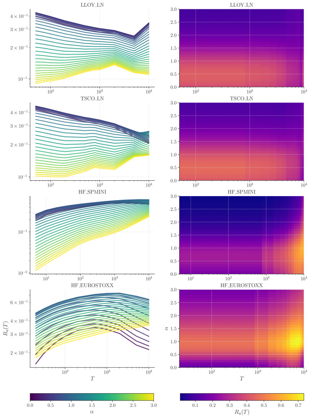
Figure 9: Analysis of the correlation function $R_{a}(T)$ for LLOY, TSCO, SPMINI and EUROSTOXX. Left column: Evolution of the correlation for different values of $a$, showing the non monotonic behavior Right column: Heatmap illustrating the distribution of correlation values within the $(a,T)$ space, indicating that the correlation reaches its peaks for $a\approx 0.5-1$, regardless of the T values.

5.7.3 Non-monotonic behaviour of $R_{a}$ vs. $a$

Finally, for point 3., Fig. 10 shows that the correlation between price returns and generalized order imbalance is non-monotonic as a function of $a$, reaching a maximum for $a^{\star}\approx 0.5$ for LLOY, TSCO and SPMINI, and $a^{\star}\approx 1$ for EUROSTOXX.

Such a non-monotonic behaviour is predicted by our theoretical analysis. Interestingly, when the diagonal contribution to $R_{a}$ dominates, we expect that the maximum correlation is reached precisely for $a^{\star}=1/2$, with a peak amplitude that decreases with $T$, see Eq. (85). The data for the two stocks is therefore compatible with the fact that in the small $a$ regime, $R_{a}(T)_{d.}$ is a decreasing function of $T$. In this regime, one can also predict that

$$\frac{R_{a=\frac{1}{2}}(T)}{R_{a=0}(T)}=e^{\sigma_{\ell}^{2}/8},$$ (89)

to be compared with the data for which this ratio is $\approx 1.1$. The inferred value of $\sigma^{2}_{\ell}$ is thus around $1$, comparable to the direct estimate of $\sigma^{2}_{\ell}$ from the variance of log-volumes, see section 3.4. The full fit of $R_{a}(T)$ vs. $a$ neglecting that the $B$ term in Eq. (85) is given in Fig. 10.

For the EUROSTOXX, on the other hand, the maximum is reached for larger values of $a$, and the ratio defined in (89) is much larger (3 – 5), suggesting that the $B(T)$ term in Eq. (88) is now dominant, as demonstrated by a fit to the data, see Fig. 10. This is consistent with our remark above – that the off-diagonal term dominates $R_{a}(T)$ for small $T$. In this scenario, the initial positive slope of $R_{a}(T)$ vs. $a$ should increase with $T$, in agreement with data. Neglecting $A(T)$ in Eq. (85) and setting $a^{\star}=1$, we now obtain

$$\frac{R_{a=1}(T)}{R_{a=0}(T)}=e^{\sigma_{\ell}^{2}(\lambda\log T-\frac{1}{2})},$$ (90)

which can indeed become large: if we take $\sigma_{\ell}^{2}=2$ and $\lambda\sigma_{\ell}^{2}=1/2$, as suggested above, one finds that for $T=100$ the ratio above is $\approx 3.7$. For $\lambda\sigma_{\ell}^{2}=1/4$, that ratio is $\approx 1.1$.

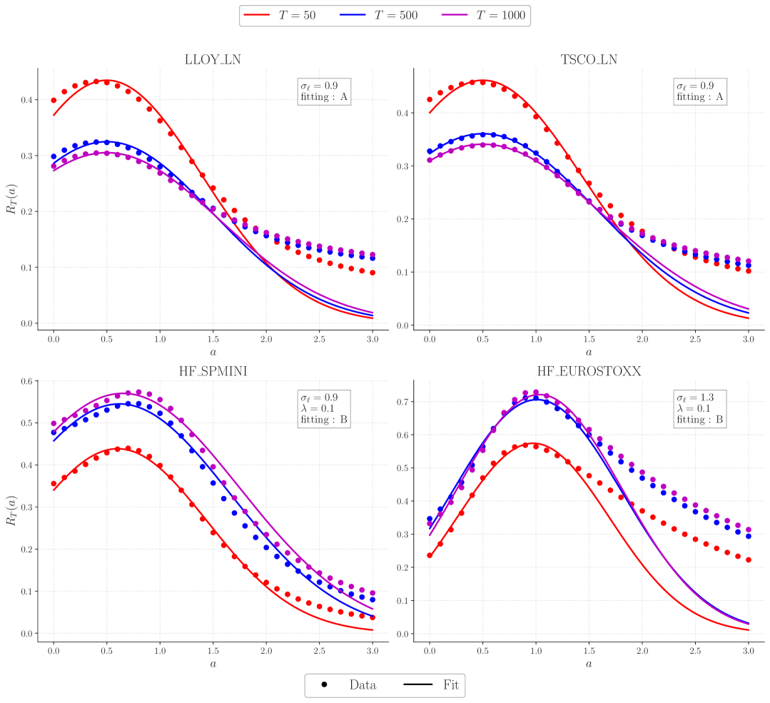
Figure 10: Fit of the correlation function $R_{a}(T)$, for several $T$. Since Eq. (88) holds only for $a<a_{c}$, we restrict the fit to $a<1.5$. The empirical estimates of $\sigma_{\ell}$ obtained with this fit turn out to be surprisingly close to the ones obtained in Fig. 1.

5.7.4 Empirical covariance: conclusion

All empirical data appear to confirm the qualitative validity of our predictions, some of them being rather non-trivial. One of the main assumptions of our model is that the exponents describing the autocorrelation of child orders ($\mu_{q}$) and the decay of their impact ($\beta_{q}$) depend on the size $q$ of these child orders. This, in turn, leads to a non-monotonic dependence of the scaling of the covariance $\operatorname{\mathbb{E}}[\Delta_{T}\cdot I_{T}^{a}]$ with $a$, and of the correlation $R_{a}(T)$ with both $T$ and $a$. Although some of our predictions fail to explain the data quantitatively, we are tempted to ascribe these discrepancies on the bluntness of our approximations, which, we argue, correctly capture the mechanisms at play.

Perhaps the two most important conclusions of this section, beyond the success of our model in capturing the main trends of the covariance data, are:

• Stocks and futures seem to differ quantitatively when it comes to the correlation between order imbalance and price changes. In particular, the correlation between the two is stronger for futures contract, and is reached for longer time intervals $T$ and with more weight given on large child order volumes (i.e. $a^{\star}=1$ instead of $a^{\star}=1/2$). This suggests a stronger role of metaorder correlations for futures than for stocks.

• The hypothesis according to which most of the volatility comes from fundamental information is hard to reconcile with the data. First, as discussed in section 4.5, this assumption does not enable one to rationalize why the square-root law, which applies to all metaorders (informed or not [53, 25, 27]) is proportional to volatility. Second, it predicts that the covariance of price returns and volume imbalances is proportional to $T$ independently of $a$, at odds with empirical data. As argued in [6, 49, 2], the most plausible hypothesis is that volatility stems from trading alone. In other words, the excess volatility puzzle has a microstructural origin.

6 Conclusion

The aim of this paper was to reconcile several apparently contradictory observations: is a square-root law of metaorder impact that decays with time compatible with the random-walk nature of prices and the linear impact of order imbalances? Can one entirely explain the volatility of prices as resulting from a “soup” of indistinguishable, randomly intertwined and uninformed metaorders?

In order to answer these questions, we have introduced a new theoretical framework to describe metaorders with different signs, sizes and durations, possibly correlated between themselves, which all impact prices as a square-root of volume (which we assume as an input) but with a subsequent time decay characterized by an exponent $\beta\neq\frac{1}{2}$, i.e. different from the one suggested by the classic propagator model [17, 2] or the LLOB model [33]. We proposed a generalized propagator model to account for such a feature.

We then established that the power-law tailed distribution of metaorder durations is not sufficient to counteract impact decay that leads to price sub-diffusion. Rather, as in the original propagator model, price diffusion is ensured by the long memory of cross-correlations between metaorders, which is indeed present in data. In fact, we conjecture that the intra- and cross-correlations between child orders decay roughly in the same manner, a feature that may be crucial for explaining the success of the construction of synthetic metaorders from public data [28].

The existence of correlations between metaorders is therefore a crucial ingredient to recover price diffusion. The old debate between order splitting and “herding” that seemed to have been closed by several papers in favor of splitting [54, 37], is perhaps not so clear-cut. Such correlations could be due either to the fact that many participants use the same trading signals, or that copy-cat metaorders/unwinding market maker inventories correlate to past order flow, or else that some traders successfully predict the future behaviour of other participants. Note that within our story any predictive alpha signal manifests itself through autocorrelated metaorders, since only trades can move the price (see also the discussion in [2], chapter 20).

In view of the strongly fluctuating volumes $q$ of child orders, one quickly realizes that one needs to account for heterogeneity in the distribution of metaorder durations, and in the resulting decay of their impact, which we parametrized by two $q$-dependent exponents, $\mu_{q}$ and $\beta_{q}$, assumed to depend linearly on $\ell=\log q$. In a nutshell, this is needed to account for the fact that metaorders with large $q$ are less autocorrelated than those with small $q$, as shown in Fig. 3. This feature allowed us to account semi-quantitatively for the way the moments of generalized volume imbalance scale with time $T$, and more importantly how the correlation between price changes and generalized volume imbalance scales with $T$. We predicted that the corresponding power-law should depend in a non-monotonic fashion on the parameter $a$ that allows one to put the same weight on all child orders ($a=0$) or overweight large orders ($a$ large), a behaviour clearly borne out by empirical data, see Fig. 8. We also predicted that the correlation between price changes and volume imbalances should display a maximum as a function of $a$ for fixed $T$, which again matches observations, see Fig. 10, with fitting parameters fixed with previously determined values. We found that stocks and futures appear to differ quite markedly in terms of these metrics, which could provide an interesting new way to characterize price formation mechanisms in different markets.

Such noteworthy agreement between theory and data suggests that our framework correctly captures the basic mechanism at the heart of price formation, namely the average impact of metaorders. We claim that our results strongly support the “Order-Driven” theory of markets, according to which it is the mechanical impact of trades, independently of any notion of “fundamental information”, that generates volatility in financial markets, a picture advocated in [6, 7, 2, 9] and, in a different context, in [8]. In particular, the Efficient Market Hypothesis, which posits that volatility is mostly due to the variation of “fundamental value”, cannot easily explain our results concerning the correlations between price changes and order flow imbalance.

All these ideas will be quantitatively confirmed in a follow-up paper (G. Maitrier et al., in preparation) using a numerical simulation of our model. Such a numerical implementation will allow us in to (i) generate realistic synthetic datasets that capture the subtle interplay between order flows and prices, and (ii) validate on such synthetic data the method of metaorder reconstruction from the public tape recently proposed in [28].

Acknowledgments

We wish to thank J. D. Farmer, J. Bonart, N. Hey, K. Kanazawa, J. Kurth, C. A. Lehalle, F. Lillo, G. Loeper, F. Patzelt, J. Ridgeway, M. Rosenbaum, Y. Sato & B. Tóth for many enlightening conversations on these topics. This research was conducted within the Econophysics & Complex Systems Research Chair, under the aegis of the Fondation du Risque, the Fondation de l’École Polytechnique and Capital Fund Management.

brokmann2015slow

References

- [1] Jean-Philippe Bouchaud “Price Impact” In Encyclopedia of Quantitative Finance Wiley Online Library, 2010
- [2] Jean-Philippe Bouchaud, Julius Bonart, Jonathan Donier and Martin Gould “Trades, quotes and prices: financial markets under the microscope” Cambridge University Press, 2018
- [3] Joel Hasbrouck “Measuring the information content of stock trades” In The Journal of Finance 46.1 Wiley Online Library, 1991, pp. 179–207
- [4] Joel Hasbrouck “Empirical market microstructure: The institutions, economics, and econometrics of securities trading” Oxford University Press, 2007
- [5] Albert S Kyle “Continuous auctions and insider trading” In Econometrica: Journal of the Econometric Society JSTOR, 1985, pp. 1315–1335
- [6] Jean-Philippe Bouchaud, Julien Kockelkoren and Marc Potters “Random walks, liquidity molasses and critical response in financial markets” In Quantitative finance 6.02 Taylor & Francis, 2006, pp. 115–123
- [7] Carl Hopman “Do supply and demand drive stock prices?” In Quantitative Finance 7.1 Taylor & Francis, 2007, pp. 37–53
- [8] Xavier Gabaix and Ralph SJ Koijen “In search of the origins of financial fluctuations: The inelastic markets hypothesis”, 2021
- [9] Jean-Philippe Bouchaud “The inelastic market hypothesis: a microstructural interpretation” In Quantitative Finance 22.10 Taylor & Francis, 2022, pp. 1785–1795
- [10] Jean-Philippe Bouchaud, J Doyne Farmer and Fabrizio Lillo “How markets slowly digest changes in supply and demand” In Handbook of financial markets: dynamics and evolution Elsevier, 2009, pp. 57–160
- [11] Philippe Beck, Jean-Philippe Bouchaud and Dario Villamaina “Ponzi funds” In arXiv preprint arXiv:2405.12768, 2024
- [12] Fischer Black “Noise” In The journal of finance 41.3 Wiley Online Library, 1986, pp. 528–543
- [13] Terrance Odean “Do investors trade too much?” In American economic review 89.5 American Economic Association, 1999, pp. 1279–1298
- [14] Robert Shiller “Do Stock Prices Move Too Much to Be Justified by Subsequent Changes in Dividends?” In American Economic Review 71, 1981, pp. 421–36
- [15] Stephen F LeRoy “Excess volatility” In The New Palgrave Dictionary of Economics, 2nd Edition. Palgrave Macmillan 13, 2006
- [16] Jutta G Kurth, Adam A Majewski and Jean-Philippe Bouchaud “Revisiting the Excess Volatility Puzzle Through the Lens of the Chiarella Model” In arXiv preprint arXiv:2505.07820, 2025
- [17] Jean-Philippe Bouchaud, Yuval Gefen, Marc Potters and Matthieu Wyart “Fluctuations and response in financial markets: thesubtle nature ofrandom’price changes” In Quantitative finance 4.2 IOP Publishing, 2003, pp. 176
- [18] Thomas F Loeb “Trading cost: the critical link between investment information and results” In Financial Analysts Journal 39.3 Taylor & Francis, 1983, pp. 39–44
- [19] Richard C Grinold and Ronald N Kahn “Active portfolio management” McGraw Hill New York, 2000
- [20] Robert Almgren, Chee Thum, Emmanuel Hauptmann and Hong Li “Direct estimation of equity market impact” In Risk 18.7, 2005, pp. 58–62
- [21] Bence Tóth et al. “Anomalous price impact and the critical nature of liquidity in financial markets” In Physical Review X 1.2 APS, 2011, pp. 021006
- [22] Emmanuel Bacry, Adrian Iuga, Matthieu Lasnier and Charles-Albert Lehalle “Market impacts and the life cycle of investors orders” In Market Microstructure and Liquidity 1.02 World Scientific, 2015, pp. 1550009
- [23] Jonathan Donier and Julius Bonart “A million metaorder analysis of market impact on the Bitcoin” In Market Microstructure and Liquidity 1.02 World Scientific, 2015, pp. 1550008
- [24] Bence Tóth, Zoltán Eisler and J-P Bouchaud “The Square-Root Impace Law Also Holds for Option Markets” In Wilmott 2016.85 Wiley Online Library, 2016, pp. 70–73
- [25] Frédéric Bucci, Michael Benzaquen, Fabrizio Lillo and Jean-Philippe Bouchaud “Slow decay of impact in equity markets: insights from the ANcerno database” In Market Microstructure and Liquidity 4.03n04 World Scientific, 2018, pp. 1950006
- [26] Andrea Frazzini, Ronen Israel and Tobias J Moskowitz “Trading costs” In Available at SSRN 3229719, 2018
- [27] Yuki Sato and Kiyoshi Kanazawa “Does the square-root price impact law belong to the strict universal scalings?: quantitative support by a complete survey of the Tokyo stock exchange market” In arXiv preprint arXiv:2411.13965, 2024
- [28] Guillaume Maitrier, Grégoire Loeper and Jean-Philippe Bouchaud “Generating realistic metaorders from public data”, 2025 arXiv: https://arxiv.org/abs/2503.18199
- [29] Kevin T Webster “Handbook of price impact modeling” ChapmanHall/CRC, 2023
- [30] Frédéric Bucci, Iacopo Mastromatteo, Michael Benzaquen and Jean-Philippe Bouchaud “Impact is not just volatility” In Quantitative Finance 19.11 Taylor & Francis (Routledge), 2019, pp. 1763–1766 DOI: 10.1080/14697688.2019.1622768
- [31] Esteban Moro et al. “Market impact and trading profile of hidden orders in stock markets” In Physical Review E—Statistical, Nonlinear, and Soft Matter Physics 80.6 APS, 2009, pp. 066102
- [32] Louis Saddier and Matteo Marsili “A Bayesian theory of market impact” In Journal of Statistical Mechanics: Theory and Experiment 2024.8 IOP Publishing, 2024, pp. 083404
- [33] Jonathan Donier, Julius Bonart, Iacopo Mastromatteo and J-P Bouchaud “A fully consistent, minimal model for non-linear market impact” In Quantitative finance 15.7 Taylor & Francis, 2015, pp. 1109–1121
- [34] Jonathan Donier and Jean-Philippe Bouchaud “From Walras’ auctioneer to continuous time double auctions: A general dynamic theory of supply and demand” In Journal of Statistical Mechanics: Theory and Experiment 2016.12 IOP Publishing, 2016, pp. 123406
- [35] Guillaume Maitrier, Grégoire Loeper, Kiyoshi Kanazawa and Jean-Philippe Bouchaud “The” double” square-root law: Evidence for the mechanical origin of market impact using Tokyo Stock Exchange data” In arXiv preprint arXiv:2502.16246, 2025
- [36] J Doyne Farmer, Austin Gerig, Fabrizio Lillo and Henri Waelbroeck “How efficiency shapes market impact” In Quantitative Finance 13.11 Taylor & Francis, 2013, pp. 1743–1758
- [37] Yuki Sato and Kiyoshi Kanazawa “Inferring microscopic financial information from the long memory in market-order flow: A quantitative test of the Lillo-Mike-Farmer model” In Physical Review Letters 131.19 APS, 2023, pp. 197401
- [38] Fabrizio Lillo, Szabolcs Mike and J Doyne Farmer “Theory for long memory in supply and demand” In Physical Review E—Statistical, Nonlinear, and Soft Matter Physics 71.6 APS, 2005, pp. 066122
- [39] Frédéric Bucci et al. “Co-impact: Crowding effects in institutional trading activity” In Quantitative Finance 20.2 Taylor & Francis, 2020, pp. 193–205
- [40] Matthieu Wyart and Jean-Philippe Bouchaud “Statistical models for company growth” In Physica A: Statistical Mechanics and its Applications 326.1–2 Elsevier BV, 2003, pp. 241–255 DOI: 10.1016/s0378-4371(03)00267-x
- [41] José Moran, Angelo Secchi and Jean-Philippe Bouchaud “Revisiting Granular Models of Firm Growth”, 2024 arXiv: https://arxiv.org/abs/2404.15226
- [42] Felix Patzelt and Jean-Philippe Bouchaud “Universal scaling and nonlinearity of aggregate price impact in financial markets” In Physical Review E 97.1 APS, 2018, pp. 012304
- [43] Paul Jusselin and Mathieu Rosenbaum “No-arbitrage implies power-law market impact and rough volatility”, 2018 arXiv: https://arxiv.org/abs/1805.07134
- [44] Frédéric Bucci, Michael Benzaquen, Fabrizio Lillo and Jean-Philippe Bouchaud “Crossover from linear to square-root market impact” In Physical review letters 122.10 APS, 2019, pp. 108302
- [45] Yuki Sato and Kiyoshi Kanazawa “Exactly solvable model of the square-root price impact dynamics under the long-range market-order correlation”, 2025 arXiv: https://arxiv.org/abs/2502.17906
- [46] Jean-François Muzy, Jean Delour and Emmanuel Bacry “Modelling fluctuations of financial time series: from cascade process to stochastic volatility model” In The European Physical Journal B-Condensed Matter and Complex Systems 17 Springer, 2000, pp. 537–548
- [47] Cecilia Aubrun, Rudy Morel, Michael Benzaquen and Jean-Philippe Bouchaud “Identifying new classes of financial price jumps with wavelets” In Proceedings of the National Academy of Sciences 122.6 National Academy of Sciences, 2025, pp. e2409156121
- [48] Matthieu Wyart et al. “Relation between bid–ask spread, impact and volatility in order-driven markets” In Quantitative finance 8.1 Taylor & Francis, 2008, pp. 41–57
- [49] Damian Eduardo Taranto et al. “Linear models for the impact of order flow on prices. I. History dependent impact models” In Quantitative Finance 18.6 Taylor & Francis, 2018, pp. 903–915
- [50] Vasiliki Plerou, Parameswaran Gopikrishnan, Xavier Gabaix and H Eugene Stanley “Quantifying stock-price response to demand fluctuations” In Physical review E 66.2 APS, 2002, pp. 027104
- [51] Martin DD Evans and Richard K Lyons “Order flow and exchange rate dynamics” In Journal of political economy 110.1 The University of Chicago Press, 2002, pp. 170–180
- [52] Tarun Chordia and Avanidhar Subrahmanyam “Order imbalance and individual stock returns: Theory and evidence” In Journal of Financial Economics 72.3 Elsevier, 2004, pp. 485–518
- [53] Carla Gomes and Henri Waelbroeck “Is market impact a measure of the information value of trades? Market response to liquidity vs. informed metaorders” In Quantitative Finance 15.5 Taylor & Francis, 2015, pp. 773–793
- [54] Bence Toth, Imon Palit, Fabrizio Lillo and J Doyne Farmer “Why is equity order flow so persistent?” In Journal of Economic Dynamics and Control 51 Elsevier, 2015, pp. 218–239