Scale-by-scale energy transfers in bubbly flows

Abstract

Variable density buoyancy-driven bubbly flows allow for multiple definitions of scale-dependent (or filtered) energy. A priori, it is not obvious which of these provide the most physically apt scale-by-scale budget. In the present study, we compare two such definitions, based on (a) filtered momentum and filtered velocity (Pandey et al., 2020), and (b) Favre filtered energy (Aluie, 2013; Pandey et al., 2023). We also derive a Kármán-Howarth-Monin (KHM) relation using the momentum-velocity correlation function and contrast it with the scale-by-scale energy budget obtained in (a). We find that irrespective of the definition, the mechanism of energy transfer is identical for the advective nonlinearity and surface tension. However, a careful investigation reveals that depending on the definition, either buoyancy or pressure can lead to transfer of energy from a scale corresponding to the bubble diameter to larger scales.

1 Introduction

The presence of bubbles is known to dramatically alter transport properties in a variety of natural and industrial flows (Clift et al., 2005; Balachandar & Eaton, 2010). Perhaps the simplest, not yet well understood, realization of such a phenomenon are the complex spatio-temporal flows (often referred to as pseudo-turbulence or bubble-induced agitation) generated by a dilute swarm of bubbles rising through an otherwise quiescent fluid (Risso, 2018; Mathai et al., 2020; Ni, 2024).

There are two salient features of incompressible, single-phase homogeneous, and isotropic turbulence (Frisch, 1995): power-law scaling of the energy spectrum $E(k)\sim k^{-5/3}$, and the cascade of energy from large to small scales in the inertial range while maintaining a constant energy flux. These are now well-established by state-of-the-art numerical simulations and experiments (Ishihara et al., 2016; Iyer et al., 2020; Küchler et al., 2023).

The key dimensionless numbers that characterize pseudo-turbulence are the Galilei number $\mbox{Ga}=\sqrt{\rho_{L}(\rho_{L}-\rho_{B})gD^{3}/\mu^{2}}$ and the Atwood number $\mbox{At}=(\rho_{L}-\rho_{B})/(\rho_{L}+\rho_{B})$, where $\rho_{l}$ is the density of the liquid phase, $\rho_{b}$ is the density of bubble, $\mu$ is the viscosity of the liquid phase, $g$ is the gravitational acceleration and $D$ is the bubble diameter. In the present work, the volume fraction and surface tension are chosen so that bubble breakups and mergers are negligible.

Experiments and numerical studies at moderate $\mbox{Ga}\,(<1000)$ and varying At characterize pseudo-turbulence by a power-law scaling of the energy spectrum $E(k)\sim k^{-\alpha}$, where the exponent $\alpha$ depends on Ga and At (Lance & Bataille, 1991; Esmaeeli & Tryggvason, 1998, 1999; Riboux et al., 2010; Mercado et al., 2010; Prakash et al., 2016; Pandey et al., 2020; Innocenti et al., 2021; Ma et al., 2022; Pandey et al., 2022; Ravisankar & Zenit, 2024). In a recent study, using high-resolution numerical simulations at large $\mbox{Ga}\,(>1000)$, Pandey et al. (2023) show that Kolmogorov turbulence coexists with pseudo-turbulence. This has been corroborated experimentally by Ma et al. (2025).

Different studies have investigated energy transfers in bubbly flows using a scale-by-scale budget equation (Pandey et al., 2020, 2023; Ramirez et al., 2024). However, as is the case for variable density flows, there is no unique way to define scale-dependent kinetic energy, making the analysis ambiguous (Aluie, 2013). Some studies (Prakash et al., 2016; Innocenti et al., 2021; Ma et al., 2022) avoid this ambiguity by focusing only on the liquid phase, where the density is constant. This, of course, misses out on the bubble phase contributions to the energy transfers.

The non-uniqueness of scale-dependent energy is not limited to bubbly flows, but is a feature of any variable-density flows. Indeed, several studies on compressible flows have earlier addressed this issue by comparing scale-by-scale budget obtained using different definitions of the large-scale energy. These studies show that different definitions of energy lead to identical qualitative picture of kinetic energy transfer mechanisms (Wang et al., 2013; Hellinger et al., 2020, 2021a, 2021b).

In this paper, we investigate scale-by-scale energy transfers in bubbly flows by using different definitions of scale-dependent energy that have been used in the literature. We follow the procedure outlined in Frisch (1995); Pope (2000); Aluie (2013) and derive the scale-by-scale budget equation for two different definitions of scale-dependent energy. For one of these definitions, we also derive an equivalent Kármán-Howarth-Monin (KHM) relation to study kinetic energy transfers in terms of spatial correlations, following Galtier & Banerjee (2011). We show that although different definitions show a net transfer of energy from large to small scales, the individual contribution to the inter-scale energy transfer do not have identical physical interpretation.

The rest of the paper is organized as follows: in Section 2 we discuss the equations of motion, next we provide an overview of different methodologies and definitions that can be used to study these flows in Section 3, the Direct Numerical Simulation (DNS) details are in Section 4. The results are presented in Section 5.

2 Model

The system is modeled by the Navier-Stokes equations in the one-phase formulation,

$$\text{D}_{t}\rho\boldsymbol{u} =-\bnabla p+\mu\nabla^{2}\boldsymbol{u}+\boldsymbol{F}^{g}+\boldsymbol{F}^{\sigma},$$ (1a)

$$\text{D}_{t}\rho =0,$$ (1b)

$$\bnabla\cdot\boldsymbol{u} =0.$$ (1c)

Here, $\boldsymbol{u}(\boldsymbol{x},\,t)$ is the hydrodynamic velocity field at location $\boldsymbol{x}=(x,y,z)$ and time $t$. For brevity, we drop the arguments and write it simply as $\boldsymbol{u}$. Likewise, $\rho$ is the density field, $p$ is pressure, $\mu$ is the dynamic viscosity assumed identical in both phases, and $\text{D}_{t}=\partial_{t}+\boldsymbol{u}\cdot\nabla$ is the material derivative. The buoyancy force is given as $\boldsymbol{F}^{g}=(\rho-\rho_{a})g\hat{\boldsymbol{z}}$, where $g$ is the gravitational acceleration, and $\rho_{a}=1/V\int\rho d\boldsymbol{x}$ is the density averaged over the volume of the domain $V$, and the surface tension force is, $\boldsymbol{F}^{\sigma}=\sigma\kappa\boldsymbol{\hat{n}}$, where $\sigma$ is the surface tension coefficient of the bubble-fluid interface, $\kappa$ is the curvature (field) and $\boldsymbol{\hat{n}}$ is the unit normal vector on the surface of the bubble.

The density field can be written as (arguments are suppressed for brevity),

$$\rho=\phi\rho_{B}+(1-\phi)(\rho_{L}-\rho_{B}),$$ (2)

where $\phi$ is the indicator function for the bubble phase, and, $\rho_{B}$ and $\rho_{L}$ are the bubble and liquid phase densities respectively. $\phi$ varies smoothly from $1$ (inside the bubble) to $0$ (in the liquid). We initialize the simulation domain with randomly distributed $N_{b}$ spherical bubbles of diameter $D$ to achieve the volume fraction $\alpha\equiv N_{b}\pi D^{3}/6L^{3}$.

3 Scale-by-Scale Energy Transfers

For any field $\psi({\bf x})$, we define the corresponding filtered field as

$$\overline{\psi}_{K}(\boldsymbol{x})=G_{r}*\psi=\int d^{3}k\,G_{K}\,\hat{\psi}e^{i\boldsymbol{k}\cdot\boldsymbol{x}},$$ (3)

where $G_{K}$ is a smooth low-pass filter that suppresses fluctuations at scales $<1/K$, $\hat{\psi}$ is the Fourier transform of $\psi$, and $r\sim 1/K$ is the filtering length scale corresponding to the filtering wavenumber $K$ (Pope, 2000; Domaradzki & Carati, 2007). In what follows, we will always use an isotropic Gaussian filter, $G_{K}(\boldsymbol{k})=\exp(-k^{2}/24K^{2})$, since it is smooth in both real space and Fourier space. Another common choice is a sharp spectral filter (Frisch, 1995), $G_{K}(\boldsymbol{k})=H(K-k)$ where $H$ is the Heavside step function. Note that because the filtering operator $G$ commutes with the derivative operator, the filtered velocity field $\overline{\boldsymbol{u}}_{K}$ is also incompressible.

Some commonly used definitions of the scale-dependent (filtered) kinetic energy used for studying either variable density or compressible flows are ($\langle\rangle$ denote spatial averaging):

• : $\mathcal{E}_{K}\equiv\frac{1}{2}\langle\overline{\rho\boldsymbol{u}}_{K}\cdot\overline{\boldsymbol{u}}_{K}\rangle$ (Graham et al., 2010; Salvesen et al., 2013; Pandey et al., 2020)

• : $\mathcal{E}_{K}\equiv\frac{1}{2}\langle\overline{\rho\boldsymbol{u}}_{K}\cdot\overline{\rho\boldsymbol{u}}_{K}/\overline{\rho}_{K}\rangle$ (Favre, 1965; Aluie, 2011; Pandey et al., 2023)

• : $\mathcal{E}_{K}\equiv\frac{1}{2}\langle\overline{\rho}_{K}\,\overline{\boldsymbol{u}}_{K}\cdot\overline{\boldsymbol{u}}_{K}\rangle$ (Chassaing, 1985)

• : $\mathcal{E}_{K}\equiv\frac{1}{2}\langle(\overline{\sqrt{\rho}\boldsymbol{u}}_{K})^{2}\rangle$ (Kida & Orszag, 1990; Miura & Kida, 1995)

Note that except for F1, the other definitions of filtered energy are positive definite by construction. For flows with extreme density variations or shocks, Aluie (2013); Zhao & Aluie (2018) have argued for the use of Favre-filtered energy F2. All the above definitions are identical for flows with uniform density $\rho(\boldsymbol{x},t)=\rho_{0}$.

Equivalently, interscale energy transfers can also be investigated from the time evolution of the appropriate two-point correlation functions by deriving the the Kármán-Howarth-Monin relation. Two commonly used correlators for variable density flows are:

• : $R(\boldsymbol{r})=\frac{1}{2}\langle\rho(\boldsymbol{x})\boldsymbol{u}(\boldsymbol{x})\cdot\boldsymbol{u}(\boldsymbol{x+r})\rangle$ (Galtier & Banerjee, 2011; Banerjee & Kritsuk, 2017)

• : $R(\boldsymbol{r})=\frac{1}{2}\langle\sqrt{\rho\boldsymbol{u}}(\boldsymbol{x})\cdot\sqrt{\rho\boldsymbol{u}}(\boldsymbol{x+r})\rangle$ (Wang et al., 2013; Hellinger et al., 2021a)

For sharp spectral filter, the derivative of the filtered energy $d\mathcal{E}_{k}/dk$ is related to the (shell-averaged) correlator as (Davidson, 2015)

$$R(r)=\int\frac{d\mathcal{E}_{k}}{dk}\frac{\sin(kr)}{kr}dk.$$ (4)

Therefore, the expression above relates the correlators with the filtered energy. It can be easily verified that C1 is related to F1, and C2 is related to F4. Some studies (Hill, 2001; Arun et al., 2021; Hamba, 2022) have previously also looked at transport equations for the correlation tensor, $R_{ij}(\boldsymbol{r})=1/2\,\langle\rho(\boldsymbol{x})u_{i}(\boldsymbol{x})u_{j}(\boldsymbol{x+r})\rangle$, identifying the (shell-averaged) scale-space energy density can be defined as $E(r)=-\partial_{r}R_{ii}(r)$.

We now summarize some choices that have been used in the past to study energy transfers in bubbly flows. Motivated by Galtier & Banerjee (2011), Pandey et al. (2020); Ramadugu et al. (2020) defined the filtered energy as F1, corresponding to the velocity-momentum correlator (C1). For bubbly flows, they show that the buoyancy contribution varies non-monotonically with respect to the filter cutoff $K$, and both pressure and advective nonlinearity contributions transfer energy from large scales to small scales. In a subsequent work, Pandey et al. (2023) used density-weighted Favre velocity to study the energy transfers, i.e., definition F2. This approach is extensively used to study scale-by-scale budget in compressible turbulence (Aluie, 2013), and leads to a (point-wise) positive definite filtered energy. For bubbly flows, the buoyancy contribution to the Favre budget is a monotonically increasing function of the filtering wavenumber $K$, the nonlinear flux shows a transfer from large scale to small scales, but the pressure contribution performs an inverse transfer. Alternatively, Ramirez et al. (2024) circumvented the need to define filtered energy by writing a spectral balance equation instead. However, this comes at the cost of containing an additional inertial time-derivative term in the budget, which has a non-zero contribution in the steady state, thus has to be interpreted carefully.

In the following, we review the scale-by-scale energy budget equations obtained using definitions F1 and F2. For F1, we derive an equivalent KHM relation for the velocity-momentum correlation using the definition C1.

3.1 Scale-by-scale budget for $\mathcal{E}_{K}=(1/2)\langle\overline{\rho\boldsymbol{u}}_{K}\cdot\overline{\boldsymbol{u}}_{K}\rangle$ (F1)

We first derive the scale-by-scale budget using the filtering approach presented in Pandey et al. (2020). Starting from the Navier-Stokes equations, we obtain the following equations for the filtered momentum,

$$\partial_{t}\overline{\rho\boldsymbol{u}}_{K}+\bnabla\cdot\overline{\rho\boldsymbol{u}\boldsymbol{u}}_{K}=-\bnabla\,\overline{p}_{K}+\mu\nabla^{2}\overline{\boldsymbol{u}}_{K}+\overline{\boldsymbol{F}^{g}}_{K}+\overline{\boldsymbol{F}^{\sigma}}_{K},$$ (5)

and the filtered velocity,

$$\partial_{t}\overline{\boldsymbol{u}}_{K}+\bnabla\cdot\overline{\boldsymbol{u}\boldsymbol{u}}_{K}=-\overline{\left(\frac{\bnabla p}{\rho}\right)}_{K}+\mu\nabla^{2}\overline{\boldsymbol{u}}_{K}+\overline{\boldsymbol{F}^{g}}_{K}+\overline{\boldsymbol{F}^{\sigma}}_{K}.$$ (6)

Taking the dot product of (5) with $\overline{\boldsymbol{u}}_{K}$, (6) with $\overline{\rho\boldsymbol{u}}_{K}$, and averaging the two we obtain the following equation for the filtered energy $\mathcal{E}_{K}$:

$$\partial_{t}\mathcal{E}_{K}=\mathcal{N}_{K}+\mathcal{D}_{K}+\mathcal{P}_{K}+\mathcal{F}^{g}_{K}+\mathcal{F}^{\sigma}_{K},$$ (7)

where $\mathcal{N}_{K}$ is the advective nonlinear contribution, $\mathcal{D}_{K}$ is the viscous dissipation, $\mathcal{P}_{K}$ is the baropycnal (pressure) contribution, $\mathcal{F}^{g}_{K}$ is the buoyancy injection and $\mathcal{F}^{\sigma}_{K}$ is the surface tension contribution. The explicit expressions for each of these contributions are given below,

$$\mathcal{N}_{K} = -\frac{1}{2}\left\langle\overline{\boldsymbol{u}}_{K}\cdot\bnabla\,\overline{\rho\boldsymbol{u}\boldsymbol{u}}_{K}+\overline{\rho\boldsymbol{u}}_{K}\cdot\bnabla\,\overline{\boldsymbol{u}\boldsymbol{u}}_{K}\right\rangle,\mathcal{F}^{a}_{K}=\frac{1}{2}\left\langle\overline{\boldsymbol{u}}_{K}\cdot\overline{\boldsymbol{F}^{a}}_{K}+\overline{\rho\boldsymbol{u}}_{K}\cdot\overline{\left(\frac{\boldsymbol{F}^{a}}{\rho}\right)}_{K}\right\rangle$$

$$\mathcal{D}_{K} = \frac{\mu}{2}\left\langle\overline{\boldsymbol{u}}_{K}\cdot\nabla^{2}\overline{\boldsymbol{u}}_{K}+\overline{\rho\boldsymbol{u}}_{K}\cdot\overline{\left(\frac{\nabla^{2}\boldsymbol{u}}{\rho}\right)}_{K}\right\rangle,~\rm{and}~\mathcal{P}_{K}=-\frac{1}{2}\left\langle\overline{\rho\boldsymbol{u}}_{K}\cdot\overline{\left(\frac{\bnabla p}{\rho}\right)}_{K}\right\rangle.$$ (8)

In the last expression, the superscript $a$ stands for $\sigma$ or $g$. The above equation reduces to the time evolution equation for the total kinetic energy $1/2\,\langle\rho u^{2}\rangle$ in the limit $K\to\infty$. Note that the contributions due to the advective nonlinearity $\mathcal{N}_{K}$ and the pressure $\mathcal{P}_{K}$ vanish in this limit.

Note that in our notation negative (positive) transfer terms indicate forward (backward) transfer of energy in scale space.

3.2 Equivalent KHM Relation using velocity-momentum correlator C1

Following Galtier & Banerjee (2011), below we derive a Kármán-Howarth-Monin (KHM) relation for the two-point momentum velocity correlator:

$$R(\boldsymbol{r})=\frac{1}{2}\langle\boldsymbol{u}(\boldsymbol{x}+\boldsymbol{r})\cdot\rho(\boldsymbol{x})\boldsymbol{u}(\boldsymbol{x})\rangle.$$ (9)

The scale-dependent kinetic energy is defined as

$$\mathcal{R}(\boldsymbol{r})=\frac{1}{2}\left[{R(\boldsymbol{r})+R(-\boldsymbol{r})}\right]=\frac{1}{4}\langle\rho\boldsymbol{u}\cdot\boldsymbol{u}^{\prime}+\rho^{\prime}\boldsymbol{u}^{\prime}\cdot\boldsymbol{u}\rangle,$$ (10)

where the superscript $(\cdot)^{\prime}$ indicates the value of function at position $\boldsymbol{x}^{\prime}$. where the superscript $(\cdot)^{\prime}$ indicates the value of function at position $\boldsymbol{x}^{\prime}$. Starting from the Navier-Stokes equations (1) and taking a dot product with the velocity field $\boldsymbol{u}^{\prime}$, we get

$$\boldsymbol{u}^{\prime}\cdot\partial_{t}\rho\boldsymbol{u}+\boldsymbol{u}^{\prime}\cdot\bnabla\cdot\rho\boldsymbol{u}\boldsymbol{u}=-\boldsymbol{u}^{\prime}\cdot\bnabla p+\boldsymbol{u}^{\prime}\cdot\mu\nabla^{2}\boldsymbol{u}+\boldsymbol{u}^{\prime}\cdot\boldsymbol{F}^{g}+\boldsymbol{u}^{\prime}\cdot\boldsymbol{F}^{\sigma}.$$ (11)

Likewise, we write equations for $\rho\boldsymbol{u}\cdot\partial_{t}\boldsymbol{u}^{\prime}$, $\boldsymbol{u}\cdot\partial_{t}\rho^{\prime}\boldsymbol{u}^{\prime}$ and $\rho^{\prime}\boldsymbol{u}^{\prime}\cdot\partial_{t}\boldsymbol{u}$. Using the above equations and after averaging over the entire domain, we get the KHM relation (see Appendix A for details):

$$\partial_{t}\mathcal{R}(\boldsymbol{r})=\mathcal{N}(\boldsymbol{r})+\mathcal{D}(\boldsymbol{r})+\mathcal{P}(\boldsymbol{r})+\mathcal{F}^{g}(\boldsymbol{r})+\mathcal{F}^{\sigma}(\boldsymbol{r}).$$ (12)

The expressions for the contributions due to advective nonlinearity $\mathcal{N}$, viscous dissipation $\mathcal{D}$, pressure $\mathcal{P}$, surface tension $\mathcal{F}^{\sigma}$, and buoyancy injection $\mathcal{F}^{g}$ are:

$$\mathcal{N}(\boldsymbol{r}) = \frac{1}{4}\bnabla_{r}\cdot\langle\delta(\rho\boldsymbol{u})\cdot\delta\boldsymbol{u}\,\delta\boldsymbol{u}\rangle,$$

$$\mathcal{D}(\boldsymbol{r}) = \frac{\mu}{4}\left\langle\boldsymbol{u}^{\prime}\cdot\nabla^{2}\boldsymbol{u}+\rho\boldsymbol{u}\cdot\frac{\nabla^{\prime 2}\boldsymbol{u}^{\prime}}{\rho^{\prime}}+\boldsymbol{u}\cdot\nabla^{\prime 2}\boldsymbol{u}^{\prime}+\rho^{\prime}\boldsymbol{u}^{\prime}\cdot\frac{\nabla^{2}\boldsymbol{u}}{\rho}\right\rangle,$$

$$\mathcal{P}(\boldsymbol{r}) = -\frac{1}{4}\left\langle\rho\boldsymbol{u}\cdot\frac{\bnabla^{\prime}p}{\rho^{\prime}}+\rho^{\prime}\boldsymbol{u}^{\prime}\cdot\frac{\bnabla p}{\rho}\right\rangle,\,\text{and}$$

$$\mathcal{F}^{a}(\boldsymbol{r}) = \frac{1}{4}\left\langle\boldsymbol{u}^{\prime}\cdot\boldsymbol{F}\,^{a}+\rho\boldsymbol{u}\cdot\frac{\boldsymbol{F}^{a}\,{}^{\prime}}{\rho^{\prime}}+\boldsymbol{u}\cdot\boldsymbol{F}^{a}\,{}^{\prime}+\rho^{\prime}\boldsymbol{u}^{\prime}\cdot\frac{\boldsymbol{F}^{a}}{\rho}\right\rangle,$$ (13)

where $a$ stands for either $g$ (buoyancy) or $\sigma$ (surface tension). We would like to highlight that the structure of the individual contributions in (3.2) is similar to that in (3.1).

The KHM relations derived for compressible flows (Galtier & Banerjee, 2011; Lai et al., 2018) are identical to (12) in the incompressible limit ($\nabla\cdot\boldsymbol{u}=0$). Furthermore, for iso-density flows, (12) reduces to the standard KHM relation (see Frisch (1995)). The isotropic sectors of the above quantities can be obtained via shell-averaging.

3.3 Scale by scale budget for Favre filtered energy $\mathcal{E}_{K}=(1/2)\langle\overline{\rho\boldsymbol{u}}_{K}\cdot\overline{\rho\boldsymbol{u}}_{K}/\overline{\rho}_{K}\rangle$ (F2)

The following discussion closely follows Pandey et al. (2023). For a field $\psi$, the corresponding Favre filtered field is defined as

$$\tilde{\psi}_{K}=\frac{\overline{\rho\psi}_{K}}{\overline{\rho}_{K}}.$$ (14)

Using the definition of Favre filtering in the Navier-Stokes equations, we obtain the following evolution equations for the the filtered density, and the filtered momentum field:

$$\partial_{t}\overline{\rho}_{K}+\nabla\cdot\overline{\rho}_{K}\widetilde{\boldsymbol{u}}_{K} = 0,~\rm{and}$$ (15)

$$\partial_{t}\overline{\rho}_{K}\widetilde{\boldsymbol{u}}_{K}+\bnabla\cdot\overline{\rho\boldsymbol{u}\boldsymbol{u}}_{K} = -\bnabla\overline{p}_{K}+\mu\nabla^{2}\overline{\boldsymbol{u}}_{K}+\overline{\boldsymbol{F}^{g}}_{K}+\overline{\boldsymbol{F}^{\sigma}}_{K}.$$ (16)

As evident from the density equation above, Favre velocity is the advection velocity for the filtered density. From the above equations, we obtain the following scale-by-scale energy budget equation:

$$\partial_{t}\mathcal{E}_{K}=\mathcal{N}_{K}+\mathcal{D}_{K}+\mathcal{P}_{K}+\mathcal{F}^{g}_{K}+\mathcal{F}^{\sigma}_{K},$$ (17)

with

$$\mathcal{E}_{K} = \langle\overline{\rho}_{K}|\tilde{\boldsymbol{u}}_{K}|^{2}\rangle/2,$$

$$\mathcal{N}_{K} = \left\langle\overline{\rho}_{K}\bnabla\,\overline{\boldsymbol{u}}_{K}:(\widetilde{\boldsymbol{u}\boldsymbol{u}}_{K}-\widetilde{\boldsymbol{u}}_{K}\,\widetilde{\boldsymbol{u}}_{K})\right\rangle$$

$$\mathcal{D}_{K} = \left\langle\mu\widetilde{\boldsymbol{u}}_{K}\cdot\nabla^{2}\overline{\boldsymbol{u}}_{K}\right\rangle$$

$$\mathcal{P}_{K} = -\left\langle\widetilde{\boldsymbol{u}}_{K}\cdot\bnabla\,\overline{p}_{K}\right\rangle,~\rm{and}$$

$$\mathcal{F}^{a}_{K} = \left\langle\widetilde{\boldsymbol{u}}_{K}\cdot\overline{\boldsymbol{F}^{a}}_{K}\right\rangle,$$ (18)

with $a$ again standing in for either buoyancy ($g$) or surface tension ($\sigma$). In the constant density limit, the F1 budget contributions (3.1) and the Favre F2 budget contributions (3.3) become identical.

4 Direct Numerical Simulations (DNS)

We numerically integrate (1) using a front-tracking method for bubble advection coupled to a psuedo-spectral flow solver for small At, and a finite-difference solver PARIS (Aniszewski et al., 2021) for large At. The details of the numerical implementation are provided in Pandey et al. (2020). We summarize the parameters of the two runs in table 1.

Runs	$N$	$L$	$N_{b}$	$\alpha$	At	Ga	Source
R1	512	2$\upi$	12	3.2%	0.04	605	R4 of (Pandey et al., 2023)
R2	504	2$\upi$	12	3.2%	0.8	1059	R8 of (Pandey et al., 2023)

Table 1: Details of the DNS data used. R1 comes from a pseudo-spectral front-tracker while R2 comes from a finite-difference based front-tracker.

A typical pseudo-color plot of a two-dimensional slice of the magnitude of the vorticity field, and the energy spectrum showing $-5/3$ and the $-3$ scaling regimes is shown in figure 1.

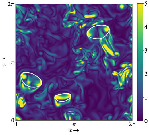
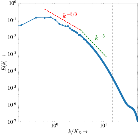
Figure 1: (a) Pseudocolor plot of the magnitude of the vorticity field $|\boldsymbol{\omega}|$ in the $y=\upi/2$ plane, and (b) energy spectrum $E(k)$ (normalized by the total kinetic energy). The dotted line indicates $k\eta=1$. Both are for run R2.

5 Results

5.1 Equivalence of the filtered budget F1 and the KHM relation C1

We first verify the equivalence of the velocity-momentum filtered budget F1 and the corresponding KHM relation with correlator C1. Different contributions to the KHM relations are evaluated by averaging the increments along the $\hat{\boldsymbol{x}}$, $\hat{\boldsymbol{y}}$ and $\hat{\boldsymbol{z}}$ directions, effectively recovering the isotropic sector.

5.1.1 Small Atwood Number $\mbox{At}=0.04$

In the small Atwood number limit ($\rho_{B}/\rho_{L}\approx 1$), we invoke the Boussinesq approximation wherein the density variations are retained only in the buoyancy term, and $\rho$ is assumed to be constant everywhere else. Note that in this regime the definitions F1 and F2 are identical. Further, pressure does not contribute to energy transfer across scales (both ${\mathcal{P}}_{K}$ in (7) and ${\mathcal{P}}(\boldsymbol{r})$ in (12) are identically zero). A side-by-side comparison of different contributions to the KHM relation and the filtered energy budget are shown in figure 2. To make the comparison evident, we have used the correspondence $Kr\sim\sqrt{3}$ (Hellinger et al., 2021a) in the KHM relation.

The different contributions obtained using the two methods show excellent agreement. The buoyancy term performs a net injection at scales comparable to bubble diameter, while the viscous term dissipates energy at small scales. The energy is transferred from the large scales to small scales through both surface tension and nonlinear advection (Pandey et al., 2020, 2023).

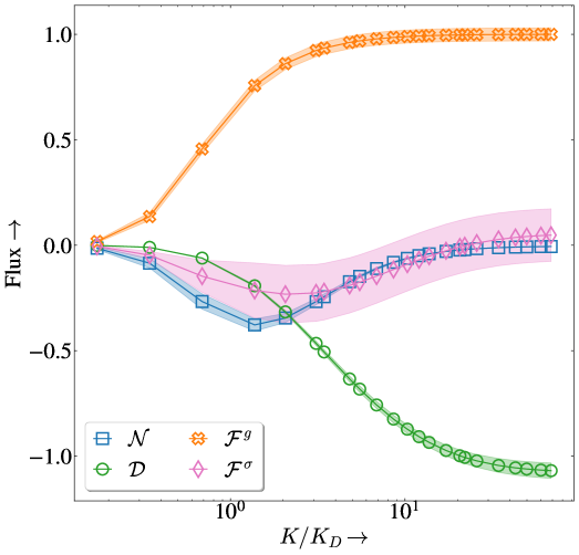
Figure 2: Scale-by-scale budget using F1 filtering (left) and the KHM relation C1 (right) for small Atwood number (run R1). The pressure contribution is identically zero, hence not shown here. The shading indicates one standard deviation variations. In both the plots, all the flux contributions (vertical axis) have been normalized by the mean energy injection rate $\epsilon^{g}\equiv\langle{\boldsymbol{u}}\cdot{\boldsymbol{F}^{g}}\rangle$.

5.1.2 Large Atwood Number $\mbox{At}=0.8$

A comparison between the filtered budget F1 and the KHM relation C1 is shown in figure 3. The excellent agreement between different contributions for the two methods is again evident. This is consistent with previous studies on compressible turbulence (Hellinger et al., 2021b).

The contributions due to the nonlinear advection, surface tension, and viscous dissipation is identical to the small At case.

However, the buoyancy contribution varies non-monotonically with the filtering wavenumber $K$. It increases up to $K\sim K_{D}$ and then decreases slightly before saturating. This suggests that the buoyancy term, in addition to the usual injection, contributes towards inter-scale transfers. Furthermore, the pressure contribution is no longer negligible, and it suggests transfers to both small and large scales from the intermediate scales. How can an injection mechanism do transfer across scales, and how can pressure simultaneously do a transfer to both large and small scales?

We do not address these questions immediately, but rather first investigate the Favre filtered F2 energy budget in the next section.

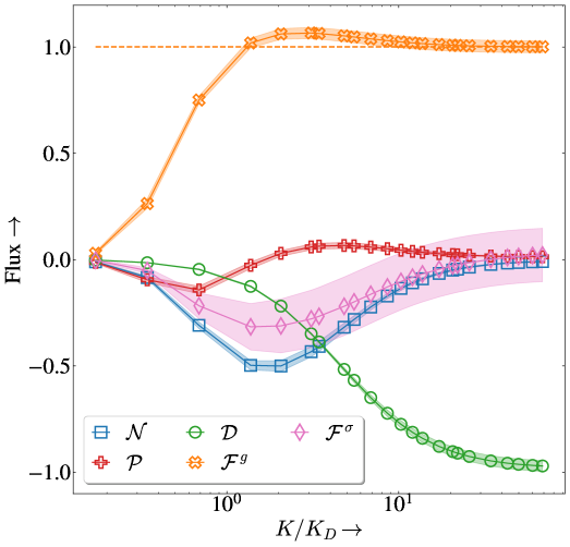
Figure 3: Scale-by-scale budget using F1 filtering (left) and the KHM relation C1 (right) for large Atwood number (run R2). The shading indicates one standard deviation variations. The orange dashed line indicates the net buoyancy injection to convey the non-monotonic behavior of the buoyant flux. In both the plots, all the flux contributions (vertical axis) have been normalized by the mean energy injection rate $\epsilon^{g}\equiv\langle{\boldsymbol{u}}\cdot{\boldsymbol{F}^{g}}\rangle$.

5.2 Favre filtered budget F2 for large Atwood number

The Favre-filtered budget for the large Atwood number case is shown in figure 4. A comparison with figure 3 reveals that the contributions of nonlinear advection transfer, viscous dissipation, and surface tension are qualitatively identical in the two cases. However, the buoyancy and pressure contributions are very different. The cumulative buoyancy injection monotonically increases saturates at large $K$ to $\mathcal{F}_{\infty}=\langle\boldsymbol{u}\cdot\boldsymbol{F}^{g}\rangle$. Perhaps the most striking is the pressure contribution, which for the Favre filtered budget performs an inverse transfer to large scales.

Previous studies on forced compressible turbulence also show, using the Favre filtered energy budget, this inverse transfer due to pressure (Wang et al., 2013; Lees & Aluie, 2019).

Notice that the sum of all the transfer terms (advection, pressure, and surface tension) is always negative, indicating that the net transfer is still from large scales to small scales.

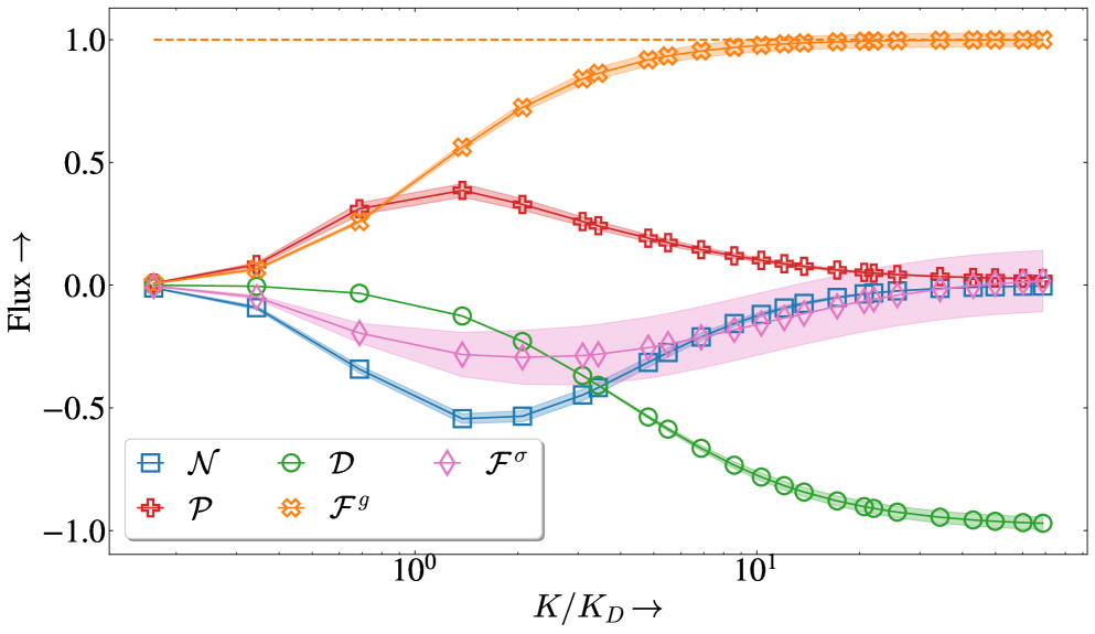
Figure 4: Scale-by-scale budget using the Favre filtering (F2) for large Atwood number (run R2). The shading indicates one standard deviation variations. All the flux contributions (vertical axis) have been normalized by the mean energy injection rate $\epsilon^{g}\equiv\langle{\boldsymbol{u}}\cdot{\boldsymbol{F}^{g}}\rangle$. In contrast with the F1 budget (figure 3), the buoyancy term increases monotonically.

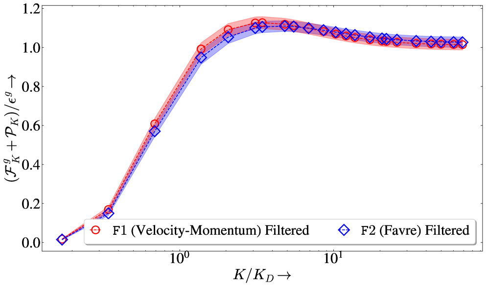
Figure 5: The sum of the baropycnal and the buoyancy contribution to the scale-by-scale budget (run R2) for both F1 and F2 definitions.

5.3 Reconciling definitions F1 and F2

Evidently, the definitions F1 and F2 for the large-scale energy give strikingly different for the buoyancy $\mathcal{F}^{g}$ and pressure $\mathcal{P}$ contributions.
Since the other contributions are similar, one finds that, not surprisingly, the sum $\mathcal{F}^{g}_{K}+\mathcal{P}_{K}$ is nearly the same in the two definitions, see figure 5.

In the Favre-filtered scheme F2, the injection $\mathcal{F}^{g}_{K}$ monotonically increases, while the non-monotonic positive pressure contribution indicates a transfer to large scales. Therefore, we argue that the non-monotonic behavior of the buoyancy term in the velocity-momentum budget F1 is because of the presence of subgrid-scale contributions that couple the large and small scales.

5.3.1 Decomposing the buoyancy contribution in F1

Recall that the buoyancy term has two contributions:

$$\mathcal{F}\,^{{\tt F1},\,g}_{K}=\underbrace{\frac{1}{2}\left\langle\overline{\boldsymbol{u}}_{K}\cdot\overline{\boldsymbol{F}^{g}}_{K}\right\rangle}_{F_{1}}+\underbrace{\frac{1}{2}\left\langle\overline{\rho\boldsymbol{u}}_{K}\cdot\overline{\left(\frac{\boldsymbol{F}^{g}}{\rho}\right)}_{K}\right\rangle}_{F_{2}}.$$

The first term $F_{1}$ is pure injection. However, we note that in $F_{2}$, the buoyancy acceleration $\overline{\boldsymbol{F}^{g}/\rho}\,_{K}$ can be further decomposed into a resolved large-scale acceleration $\overline{\boldsymbol{F}^{g}}_{K}/{\overline{\rho}}_{K}$ and a residual (sub-grid) contribution $\overline{\boldsymbol{F}^{g}/\rho}\,_{K}-\overline{\boldsymbol{F}^{g}}_{K}/{\overline{\rho}}_{K}$ as shown below:

$$2F_{2} =\left\langle\overline{\rho\boldsymbol{u}}_{K}\cdot\overline{\left(\frac{\boldsymbol{F}^{g}}{\rho}\right)}_{K}\right\rangle$$

$$=\left\langle\overline{\rho\boldsymbol{u}}_{K}\cdot\frac{\overline{\boldsymbol{F}^{g}}_{K}}{\overline{\rho}_{K}}\right\rangle+\left\langle\overline{\rho\boldsymbol{u}}_{K}\cdot\left[\overline{\left(\frac{\boldsymbol{F}^{g}}{\rho}\right)}_{K}-\frac{\overline{\boldsymbol{F}^{g}}_{K}}{\overline{\rho}_{K}}\right]\right\rangle.$$ (19)

On inspection, it is clear that the first term in the RHS is identical to the Favre filtered buoyancy contribution $\langle\widetilde{\boldsymbol{u}}_{K}\cdot\overline{\boldsymbol{F^{g}}}_{K}\rangle$, which only contributes to the injection as shown in figure 3. The second term contributes to the transfer. Indeed, if we add the residual contribution in the buoyancy to the pressure transfer, we get the following modified equation for the F1 budget

$$\partial_{t}\mathcal{E}_{K}=\mathcal{N}_{K}+\mathcal{D}_{K}+\mathcal{P}\,^{m}_{K}+\mathcal{F}^{g,\,m}_{K}+\mathcal{F}^{\sigma}_{K},$$ (20)

with the following definitions of the modified buoyancy and pressure terms,

$$\mathcal{F}^{g,\,m}_{K} = \frac{1}{2}\left\langle\overline{\boldsymbol{u}}_{K}\cdot\overline{\boldsymbol{F}^{g}}_{K}+\overline{\rho\boldsymbol{u}}_{K}\cdot\frac{\overline{\boldsymbol{F}^{g}}_{K}}{\overline{\rho}_{K}}\right\rangle,~{\rm and}$$

$$\mathcal{P}^{m}_{K} = -\frac{1}{2}\left\langle\overline{\rho\boldsymbol{u}}_{K}\cdot\overline{\left(\frac{\bnabla p}{\rho}\right)}_{K}\right\rangle+\left\langle\overline{\rho\boldsymbol{u}}_{K}\cdot\left[\overline{\left(\frac{\boldsymbol{F}^{g}}{\rho}\right)}_{K}-\frac{\overline{\boldsymbol{F}^{g}}_{K}}{\overline{\rho}_{K}}\right]\right\rangle.$$ (21)

The superscript $m$ indicates modified quantities. With these new definitions, in figure 6, we plot the modified budget. Now, all the transfers are consistent with the Favre-filtered framework. In particular, the injection term monotonically increases, but the transfer due to modified pressure is indeed from small-scale to large-scale.

Thus, on correctly identifying the residual transfer terms and the pure injection contributions, we find that both the definitions of evaluating the budget give similar results.

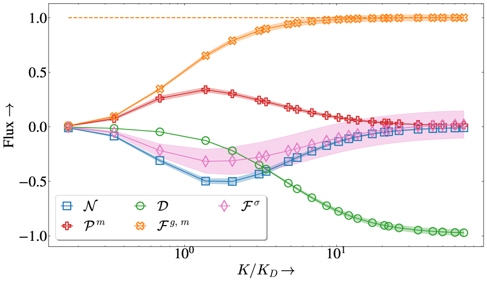
Figure 6: F1 filtered scale-by-scale budget for the large Atwood number run R2 with the modified pressure and buoyancy contributions (as in (5.3.1)). The shading indicates one standard deviation variations. $y$-axis has been normalized with the mean injection. Notice the monotonic behavior of the buoyancy term, contrast with figure 3. Further, the pressure term $\mathcal{P}$ now transfers energy definitively from small to large scales.

6 Discussion and conclusion

In this paper, we compared the scale-by-scale energy transfers obtained using two different definitions of the filtered energy, $\mathcal{E}^{\tt F1}_{K}=\langle\overline{\boldsymbol{u}}_{K}\cdot\overline{\rho\boldsymbol{u}}_{K}\rangle/2$ (velocity-momentum definition) and $\mathcal{E}^{\tt F2}_{K}=\langle{\overline{\rho}_{K}}|\widetilde{\boldsymbol{u}}_{K}|^{2}\rangle/2$ (Favre definition) for bubbly flows. For the former definition of energy transfer, we also identify an equivalent KHM relation in terms of the velocity-momentum correlation function (Galtier & Banerjee, 2011).

While the nonlinear advection, surface tension and viscous contributions to the budget seem to be robust with respect to the choice of definition of the filtered energy, the buoyancy and baropycnal (pressure) contributions are found to be significantly different.

In the Favre definition, the baropycnal term does an inverse transfer from small to large scales, while the buoyancy term is a pure injection term (Pandey et al., 2023). In contrast, in the velocity-momentum F1 definition, the pressure term transfers energy to bubble scales from both large and small scales. Furthermore, the buoyancy contribution is non-monotonic indicating that along with the energy injection at the wave number $K_{D}$, it also transfers energy from small to large scales (see figure 3). We show that the transfers obtained using the equivalent KHM relation (C1) are identical to the F1 velocity-momentum filtered budget, consistent with the previous results obtained by Hellinger et al. (2021b).

Although it is clear that both definitions contain an inverse transfer mechanism, in definition F1 this contribution is from the buoyancy term, while in definition F2 it is by the pressure term. In particular, in the final section we reconcile the definition F1 by identifying the injection and transfer contributions to the buoyancy term. We then define a modified pressure that also contains the contribution owing to buoyancy transfer.

Previously, Eyink & Drivas (2018) has criticized the use of the Galtier & Banerjee (2011) formalism for general compressible flows because in the $\mbox{Re}_{\lambda}\to\infty$ limit terms lik $\bnabla\cdot\boldsymbol{u}$ are not well defined. However, as they themselves point out, this criticism is not valid in the incompressible regime $\nabla\cdot{\boldsymbol{u}}=0$, which is of interest to the present study.

The earlier study Kritsuk et al. (2013) on forced compressible homogeneous and isotropic turbulence (CHIT) that employed the velocity-momentum KHM relation to the study energy transfers did not observe any transfer mechanism in injection. While the injection terms like $\langle\boldsymbol{u}^{\prime}\cdot\boldsymbol{F}\rangle$ are, in general, functions of $\boldsymbol{r}$, Kritsuk et al. (2013) argue that for their choice of forcing and compressible flow dynamics, the injection terms are essentially constant in the inertial range. This follows from their observation that the density field has a very short correlation length. Crucially, in our study, this assumption is not valid since the bubbles represent large-scale coherent density structures of size $D\approx L/5$ where $L$ is the size of the box. Hence, for bubbly flows the buoyancy contribution may couple different length scales within the KHM framework (C1).

To conclude, we compare and contrast two different definitions for the filtered energy F1 and F2 for incompressible bubbly flows. Our findings reinforce the conclusions presented in Pandey et al. (2023), where the non-zero contribution of the baropycnal term was noted. We find that an inverse transfer exists in both the schemes, however, different physical mechanisms are responsible for it in the two schemes (buoyancy in F1 and pressure in F2). The net transfer continues on large to small scales. The differences in the mechanisms is not necessarily a surprising result, given that the two filtered energy definitions are different. However, our study highlights the importance of identifying relevant transfer mechanisms that control physics at different scales in buoyancy driven bubbly flows.

[Acknowledgements]HPC facility at TIFR Hyderabad.

[Funding]D. M. and V. P. acknowledge the support of the Swedish Research Council Grants No. 638-2013-9243 and No. 2016-05225. Nordita is partially supported by Nordforsk. H.N. and P. P. acknowledge support from the Department of Atomic Energy (DAE), India under Project Identification No. RTI 4007, and DST (India) Projects No. MTR/2022/000867.

[Declaration of interests]The authors report no conflict of interest.

Appendix A Derivation of the Kármán-Howarth-Monin Relation

Our derivation for the KHM relation with the velocity-momentum correlator (definition C1) follows closely the presentation given in Galtier & Banerjee (2011). We first derive the time evolution equation for $R(\boldsymbol{r})=\frac{1}{2}\langle\boldsymbol{u}^{\prime}\cdot\rho\boldsymbol{u}\rangle$ Starting from the Navier-Stokes equations,

$$D_{t}\rho\boldsymbol{u}=-\bnabla p+\mu\nabla^{2}\boldsymbol{u}+\boldsymbol{F}^{g}+\boldsymbol{F}^{\sigma},$$ (22)

and taking the dot product of the above equation with $\boldsymbol{u}^{\prime}$ we get,

$$\boldsymbol{u}^{\prime}\cdot\partial_{t}\rho\boldsymbol{u}+\boldsymbol{u}^{\prime}\cdot(\bnabla\cdot\rho\boldsymbol{u}\boldsymbol{u})=-\boldsymbol{u}^{\prime}\cdot\bnabla p+\mu\boldsymbol{u}^{\prime}\cdot\nabla^{2}\boldsymbol{u}+\boldsymbol{u}^{\prime}\cdot\boldsymbol{F}^{g}+\boldsymbol{u}^{\prime}\cdot\boldsymbol{F}^{\sigma}.$$ (23)

The complementary equation to the above comes from the time evolution equation for the primed velocity field $\boldsymbol{u}^{\prime}$,

$$\rho\boldsymbol{u}\cdot\partial_{t}\boldsymbol{u}^{\prime}+\rho\boldsymbol{u}\cdot(\bnabla^{\prime}\cdot\boldsymbol{u}^{\prime}\boldsymbol{u}^{\prime})=-\rho\boldsymbol{u}\cdot\frac{\bnabla^{\prime}p^{\prime}}{\rho^{\prime}}+\mu\rho\boldsymbol{u}\cdot\frac{1}{\rho^{\prime}}\nabla^{\prime 2}\boldsymbol{u}^{\prime}+\rho\boldsymbol{u}\cdot\frac{1}{\rho^{\prime}}\boldsymbol{F}^{g}\,{}^{\prime}+\rho\boldsymbol{u}\cdot\frac{1}{\rho^{\prime}}\boldsymbol{F}^{\sigma}\,{}^{\prime}.$$ (24)

Note that for any function $f(\boldsymbol{x}+\boldsymbol{r})=f^{\prime}$, we have $\nabla^{\prime}f^{\prime}=\nabla f^{\prime}=\nabla_{r}f^{\prime}$ by chain rule. Here, $\nabla_{i}=\partial/\partial x_{i}$, $\nabla^{\prime}_{i}=\partial/\partial x^{\prime}_{i}$ and $\nabla_{ri}=\partial/\partial r_{i}$. Adding the above two equations, we have,

$$\partial_{t}(\rho\boldsymbol{u}\cdot\boldsymbol{u}^{\prime}) = -\boldsymbol{u}^{\prime}\cdot(\bnabla\cdot\rho\boldsymbol{u}\boldsymbol{u})-\rho\boldsymbol{u}\cdot(\bnabla\cdot\boldsymbol{u}^{\prime}\boldsymbol{u}^{\prime})-\boldsymbol{u}^{\prime}\cdot\bnabla p-\rho\boldsymbol{u}\cdot\frac{\bnabla p^{\prime}}{\rho^{\prime}}$$ (25)

$$+ \mu\boldsymbol{u}^{\prime}\cdot\nabla^{2}\boldsymbol{u}+\mu\rho\boldsymbol{u}\cdot\frac{1}{\rho^{\prime}}\nabla^{2}\boldsymbol{u}^{\prime}+\boldsymbol{u}^{\prime}\cdot\boldsymbol{F}+\rho\boldsymbol{u}\cdot\frac{1}{\rho^{\prime}}\boldsymbol{F}^{\prime}.$$ (26)

Here, we are using $\boldsymbol{F}$ as shorthand for $\boldsymbol{F}^{g}+\boldsymbol{F}^{\sigma}$.
We add the above equation the time evolution equation for $R(-\boldsymbol{r})$ and define the scale energy $\mathcal{R}(\boldsymbol{r})$ as,

$$\mathcal{R}=\frac{1}{4}\langle\rho\boldsymbol{u}\cdot\boldsymbol{u}^{\prime}+\rho^{\prime}\boldsymbol{u}^{\prime}\cdot\boldsymbol{u}\rangle.$$ (27)

In the limit $r\to 0$, the above definition of scale energy reduces to the mean kinetic energy. Any generic term $\boldsymbol{Q}$ that appears on the right-hand-side of the Navier-Stokes equation (for example the dissipation term $\mu\nabla^{2}\boldsymbol{u}$) has a contribution $\mathcal{Q}$ to the KHM relation that can be written as follows,

$$4\mathcal{Q}=\left\langle\boldsymbol{u}^{\prime}\cdot\boldsymbol{Q}+\rho\boldsymbol{u}\cdot\frac{\boldsymbol{Q}^{\prime}}{\rho^{\prime}}+\boldsymbol{u}\cdot\boldsymbol{Q}^{\prime}+\rho^{\prime}\boldsymbol{u}^{\prime}\cdot\frac{\boldsymbol{Q}}{\rho}\right\rangle.$$ (28)

Here also we have two types of terms - of type velocity times force, and momentum times acceleration. We can also rewrite this in terms of increments. Let $\delta$ represent increments in any quantity $\psi$, defined as,

$$\delta\psi(\boldsymbol{x},\,\boldsymbol{r})=\psi(\boldsymbol{x}+\boldsymbol{r})-\psi(\boldsymbol{x}).$$ (29)

It is then straightforward to check,

$$\left\langle\delta\boldsymbol{u}\cdot\delta\boldsymbol{Q}\right\rangle=\left\langle\boldsymbol{u}^{\prime}\cdot\boldsymbol{Q}^{\prime}+\boldsymbol{u}\cdot\boldsymbol{Q}-\boldsymbol{u}^{\prime}\cdot\boldsymbol{Q}-\boldsymbol{u}\cdot\boldsymbol{Q}^{\prime}\right\rangle.$$ (30)

The first two terms are identical after averaging over the entire box, and the last two terms correspond to the first and third term of eq. (28) (with an extra minus sign here). Therefore, we can write,

$$\mathcal{Q}=\langle\boldsymbol{u}\cdot\boldsymbol{Q}\rangle-\frac{1}{4}\left[\left\langle\delta\boldsymbol{u}\cdot\delta\boldsymbol{Q}\right\rangle+\left\langle\delta(\rho\boldsymbol{u})\cdot\delta\left(\frac{\boldsymbol{Q}}{\rho}\right)\right\rangle\right].$$ (31)

By writing the $\mathcal{Q}$ contribution like this, we cleanly separate the mean contribution (from $r=0$) and the $r>0$ contributions. In particular, the nonlinear term can be written as divergence of a third-order structure function. The nonlinear contribution, $\mathcal{N}$ is given by,

$$4\mathcal{N}=\left\langle-\boldsymbol{u}^{\prime}\cdot(\bnabla\cdot\rho\boldsymbol{u}\boldsymbol{u})-\rho\boldsymbol{u}\cdot(\bnabla\cdot\boldsymbol{u}^{\prime}\boldsymbol{u}^{\prime})-\boldsymbol{u}\cdot(\bnabla\cdot\rho^{\prime}\boldsymbol{u}^{\prime}\boldsymbol{u}^{\prime})-\rho^{\prime}\boldsymbol{u}^{\prime}\cdot(\bnabla\cdot\boldsymbol{u}\boldsymbol{u})\right\rangle$$ (32)

Consider now the following expression,

$$\bnabla_{r}\cdot\langle[\delta(\rho\boldsymbol{u})\cdot\delta\boldsymbol{u}\delta\boldsymbol{u}]\rangle.$$ (33)

The expansion of the above term gives us 8 terms,

$$\bnabla_{r}\cdot\langle[\delta(\rho\boldsymbol{u})\cdot\delta\boldsymbol{u}\delta\boldsymbol{u}]\rangle = \bnabla_{r}\cdot\langle[\rho^{\prime}\boldsymbol{u}^{\prime}\cdot\boldsymbol{u}^{\prime}\boldsymbol{u}^{\prime}$$ (34)

$$- \rho^{\prime}\boldsymbol{u}^{\prime}\cdot\boldsymbol{u}^{\prime}\boldsymbol{u}-\rho^{\prime}\boldsymbol{u}^{\prime}\cdot\boldsymbol{u}\boldsymbol{u}^{\prime}-\rho\boldsymbol{u}\cdot\boldsymbol{u}^{\prime}\boldsymbol{u}^{\prime}$$ (35)

$$+ \rho^{\prime}\boldsymbol{u}^{\prime}\cdot\boldsymbol{u}\boldsymbol{u}+\rho\boldsymbol{u}\cdot\boldsymbol{u}^{\prime}\boldsymbol{u}+\rho\boldsymbol{u}\cdot\boldsymbol{u}\boldsymbol{u}^{\prime}$$ (36)

$$- \rho\boldsymbol{u}\cdot\boldsymbol{u}\boldsymbol{u}]\rangle.$$ (37)

Note that the first and last terms cancel exactly after averaging. Terms 2 and 7 also vanish because of incompressiblity constraint. The remaining terms can be seen to be exactly $4\mathcal{N}$, by noting that,

$$\langle\bnabla_{r}\cdot(\rho^{\prime}\boldsymbol{u}^{\prime})\cdot\boldsymbol{u}\boldsymbol{u}\rangle=\langle\bnabla\cdot(\rho^{\prime}\boldsymbol{u}^{\prime})\cdot\boldsymbol{u}\boldsymbol{u}\rangle=-\langle\rho^{\prime}\boldsymbol{u}^{\prime}\cdot\bnabla\cdot\boldsymbol{u}\boldsymbol{u}\rangle,$$ (38)

hence, finally,

$$\mathcal{N}=\frac{1}{4}\bnabla_{r}\cdot\langle\delta(\rho\boldsymbol{u})\cdot\delta\boldsymbol{u}\,\delta\boldsymbol{u}\rangle.$$ (39)

Here the divergence operator acts on the scale-space coordinates $r$, not the physical space coordinates. The Kármán-Howarth-Monin relation for incompressible variable-density flows then is,

$$\partial_{t}\mathcal{R}=\mathcal{N}+\mathcal{D}+\mathcal{P}+\mathcal{F}^{g}+\mathcal{F}^{\sigma},$$ (40)

with, $\mathcal{R}=\frac{1}{4}\langle\rho\boldsymbol{u}\cdot\boldsymbol{u}^{\prime}+\rho^{\prime}\boldsymbol{u}^{\prime}\cdot\boldsymbol{u}\rangle$ being the cumulative energy in eddies larger than $r$. In the above derivation, we did not assume either homogeneity or isotropy. The above derivation can also be derived by interpreting $\langle(\ldots)\rangle$ as ensemble averaging if the flow is assumed to be homogeneous, as is the approach in Frisch (1995).

References

- Aluie (2011) Aluie, Hussein 2011 Compressible turbulence: The cascade and its locality. Phys. Rev. Lett. 106, 174502.
- Aluie (2013) Aluie, Hussein 2013 Scale decomposition in compressible turbulence. Physica D: Nonlinear Phenomena 247 (1), 54–65.
- Aniszewski et al. (2021) Aniszewski, W., Arrufat, T., Crialesi-Esposito, M., Dabiri, S., Fuster, D., Ling, Y., Lu, J., Malan, L., Pal, S., Scardovelli, R., Tryggvason, G., Yecko, P. & Zaleski, S. 2021 Parallel, robust, interface simulator (paris). Computer Physics Communications 263, 107849.
- Arun et al. (2021) Arun, S., Sameen, A., Srinivasan, Balaji & Girimaji, Sharath S. 2021 Scale-space energy density function transport equation for compressible inhomogeneous turbulent flows. J. Fluid Mech. 920, A31.
- Balachandar & Eaton (2010) Balachandar, S. & Eaton, John K. 2010 Turbulent dispersed multiphase flow. Annu. Rev. Fluid Mech. 42 (Volume 42, 2010), 111–133.
- Banerjee & Kritsuk (2017) Banerjee, Supratik & Kritsuk, Alexei G. 2017 Exact relations for energy transfer in self-gravitating isothermal turbulence. Phys. Rev. E 96, 053116.
- Chassaing (1985) Chassaing, P. 1985 An alternative formulation of the equations of turbulent motion for a fluid of variable density. Journal de Mecanique Theorique et Appliquee 4 (3), 375–389.
- Clift et al. (2005) Clift, R., Grace, J.R. & Weber, M.E. 2005 Bubbles, Drops, and Particles. Dover Publications.
- Davidson (2015) Davidson, Peter 2015 Turbulence: An Introduction for Scientists and Engineers. Oxford University Press.
- Domaradzki & Carati (2007) Domaradzki, J. Andrzej & Carati, Daniele 2007 A comparison of spectral sharp and smooth filters in the analysis of nonlinear interactions and energy transfer in turbulence. Phys. Fluids. 19 (8), 085111.
- Esmaeeli & Tryggvason (1998) Esmaeeli, Asghar & Tryggvason, Grétar 1998 Direct numerical simulations of bubbly flows. part 1. low reynolds number arrays. J. Fluid Mech. 377, 313–345.
- Esmaeeli & Tryggvason (1999) Esmaeeli, Asghar & Tryggvason, Grétar 1999 Direct numerical simulations of bubbly flows part 2. moderate reynolds number arrays. J. Fluid Mech. 385, 325–358.
- Eyink & Drivas (2018) Eyink, Gregory L. & Drivas, Theodore D. 2018 Cascades and dissipative anomalies in compressible fluid turbulence. Phys. Rev. X 8, 011022.
- Favre (1965) Favre, A. J. 1965 The equations of compressible turbulent gases. Annual Summary Report .
- Frisch (1995) Frisch, Uriel 1995 Turbulence: The Legacy of A. N. Kolmogorov. Cambridge University Press.
- Galtier & Banerjee (2011) Galtier, Sébastien & Banerjee, Supratik 2011 Exact relation for correlation functions in compressible isothermal turbulence. Phys. Rev. Lett. 107, 134501.
- Graham et al. (2010) Graham, Jonathan Pietarila, Cameron, Robert & Schüssler, Manfred 2010 Turbulent small-scale dynamo action in solar surface simulations. ApJ 714 (2), 1606.
- Hamba (2022) Hamba, Fujihiro 2022 Scale-space energy density for inhomogeneous turbulence based on filtered velocities. J. Fluid Mech. 931, A34.
- Hellinger et al. (2021a) Hellinger, Petr, Papini, Emanuele, Verdini, Andrea, Landi, Simone, Franci, Luca, Matteini, Lorenzo & Montagud-Camps, Victor 2021a Spectral transfer and kármán–howarth–monin equations for compressible hall magnetohydrodynamics. The Astrophysical Journal 917 (2), 101.
- Hellinger et al. (2020) Hellinger, Petr, Verdini, Andrea, Landi, Simone, Franci, Luca, Papini, Emanuele & Matteini, Lorenzo 2020 On cascade of kinetic energy in compressible hydrodynamic turbulence, arXiv: 2004.02726.
- Hellinger et al. (2021b) Hellinger, Petr, Verdini, Andrea, Landi, Simone, Papini, Emanuele, Franci, Luca & Matteini, Lorenzo 2021b Scale dependence and cross-scale transfer of kinetic energy in compressible hydrodynamic turbulence at moderate reynolds numbers. Phys. Rev. Fluids 6, 044607.
- Hill (2001) Hill, Reginald J. 2001 Equations relating structure functions of all orders. J. Fluid Mech. 434, 379–388.
- Innocenti et al. (2021) Innocenti, Alessio, Jaccod, Alice, Popinet, Stéphane & Chibbaro, Sergio 2021 Direct numerical simulation of bubble-induced turbulence. J. Fluid Mech. 918, A23.
- Ishihara et al. (2016) Ishihara, Takashi, Morishita, Koji, Yokokawa, Mitsuo, Uno, Atsuya & Kaneda, Yukio 2016 Energy spectrum in high-resolution direct numerical simulations of turbulence. Phys. Rev. Fluids 1, 082403.
- Iyer et al. (2020) Iyer, Kartik P., Sreenivasan, Katepalli R. & Yeung, P. K. 2020 Scaling exponents saturate in three-dimensional isotropic turbulence. Phys. Rev. Fluids 5, 054605.
- Kida & Orszag (1990) Kida, Shigeo & Orszag, Steven A. 1990 Energy and spectral dynamics in forced compressible turbulence. J. Sci. Comput. 5 (2), 85–125.
- Kritsuk et al. (2013) Kritsuk, Alexei G., Wagner, Rick & Norman, Michael L. 2013 Energy cascade and scaling in supersonic isothermal turbulence. J. Fluid Mech. 729, R1.
- Küchler et al. (2023) Küchler, Christian, Bewley, Gregory P. & Bodenschatz, Eberhard 2023 Universal velocity statistics in decaying turbulence. Phys. Rev. Lett. 131, 024001.
- Lai et al. (2018) Lai, Chris C. K., Charonko, John J. & Prestridge, Katherine 2018 A kármán–howarth–monin equation for variable-density turbulence. J. Fluid Mech. 843, 382–418.
- Lance & Bataille (1991) Lance, M. & Bataille, J. 1991 Turbulence in the liquid phase of a uniform bubbly air–water flow. J. Fluid Mech. 222, 95–118.
- Lees & Aluie (2019) Lees, Aarne & Aluie, Hussein 2019 Baropycnal work: A mechanism for energy transfer across scales. Fluids 4 (2).
- Ma et al. (2022) Ma, Tian, Hessenkemper, Hendrik, Lucas, Dirk & Bragg, Andrew D. 2022 An experimental study on the multiscale properties of turbulence in bubble-laden flows. J. Fluid Mech. 936, A42.
- Ma et al. (2025) Ma, Tian, Tan, Shiyong, Ni, Rui, Hessenkemper, Hendrik & Bragg, Andrew D. 2025 Kolmogorov scaling in bubble-induced turbulence. (to appear in) Phys. Rev. Lett. .
- Mathai et al. (2020) Mathai, Varghese, Lohse, Detlef & Sun, Chao 2020 Bubbly and buoyant particle–laden turbulent flows. Annu. Rev. Condens. Matter Phys. 11, 529–559.
- Mercado et al. (2010) Mercado, J. Martinez, Chehata Gómez, Daniel, Van Gils, Dennis, Sun, Chao & Lohse, Detlef 2010 On bubble clustering and energy spectra in pseudo-turbulence. J. Fluid Mech. 650, 287–306.
- Miura & Kida (1995) Miura, Hideaki & Kida, Shigeo 1995 Acoustic energy exchange in compressible turbulence. Phys. Fluids. 7 (7), 1732–1742.
- Ni (2024) Ni, Rui 2024 Deformation and breakup of bubbles and drops in turbulence. Annu. Rev. Fluid Mech. 56, 319–347.
- Pandey et al. (2022) Pandey, Vikash, Mitra, Dhrubaditya & Perlekar, Prasad 2022 Turbulence modulation in buoyancy-driven bubbly flows. J. Fluid Mech. 932, A19.
- Pandey et al. (2023) Pandey, Vikash, Mitra, Dhrubaditya & Perlekar, Prasad 2023 Kolmogorov turbulence coexists with pseudo-turbulence in buoyancy-driven bubbly flows. Phys. Rev. Lett. 131, 114002.
- Pandey et al. (2020) Pandey, Vikash, Ramadugu, Rashmi & Perlekar, Prasad 2020 Liquid velocity fluctuations and energy spectra in three-dimensional buoyancy-driven bubbly flows. J. Fluid Mech. 884, R6.
- Pope (2000) Pope, Stephen B. 2000 Turbulent Flows. Cambridge University Press.
- Prakash et al. (2016) Prakash, Vivek N., Martínez Mercado, J., van Wijngaarden, Leen, Mancilla, E., Tagawa, Y., Lohse, Detlef & Sun, Chao 2016 Energy spectra in turbulent bubbly flows. J. Fluid Mech. 791, 174–190.
- Ramadugu et al. (2020) Ramadugu, Rashmi, Pandey, Vikash & Perlekar, Prasad 2020 Pseudo-turbulence in two-dimensional buoyancy-driven bubbly flows: A dns study. Eur. Phys. J. E 43.
- Ramirez et al. (2024) Ramirez, Gabriel, Burlot, Alan, Zamansky, Rémi, Bois, Guillaume & Risso, Frédéric 2024 Spectral analysis of dispersed multiphase flows in the presence of fluid interfaces. International Journal of Multiphase Flow 177, 104860.
- Ravisankar & Zenit (2024) Ravisankar, Mithun & Zenit, Roberto 2024 Velocity fluctuations for bubbly flows at small re. J. Fluid Mech. 1001, A34.
- Riboux et al. (2010) Riboux, Guillaume, Risso, Frédéric & Legendre, Dominique 2010 Experimental characterization of the agitation generated by bubbles rising at high reynolds number. J. Fluid Mech. 643, 509–539.
- Risso (2018) Risso, Frédéric 2018 Agitation, mixing, and transfers induced by bubbles. Annu. Rev. Fluid Mech. 50 (Volume 50, 2018), 25–48.
- Salvesen et al. (2013) Salvesen, Greg, Beckwith, Kris, Simon, Jacob B., O’Neill, Sean M. & Begelman, Mitchell C. 2013 Quantifying energetics and dissipation in magnetohydrodynamic turbulence. Monthly Notices of the Royal Astronomical Society 438 (2), 1355–1376.
- Wang et al. (2013) Wang, Jianchun, Yang, Yantao, Shi, Yipeng, Xiao, Zuoli, He, X. T. & Chen, Shiyi 2013 Cascade of kinetic energy in three-dimensional compressible turbulence. Phys. Rev. Lett. 110, 214505.
- Zhao & Aluie (2018) Zhao, Dongxiao & Aluie, Hussein 2018 Inviscid criterion for decomposing scales. Phys. Rev. Fluids 3, 054603.