Training Superior Sparse Autoencoders for Instruct Models

Abstract

As large language models (LLMs) grow in scale and capability, understanding their internal mechanisms becomes increasingly critical. Sparse autoencoders (SAEs) have emerged as a key tool in mechanistic interpretability, enabling the extraction of human-interpretable features from LLMs. However, existing SAE training methods are primarily designed for base models, resulting in reduced reconstruction quality and interpretability when applied to instruct models. To bridge this gap, we propose Finetuning-aligned Sequential Training (FAST), a novel training method specifically tailored for instruct models. FAST aligns the training process with the data distribution and activation patterns characteristic of instruct models, resulting in substantial improvements in both reconstruction and feature interpretability. On Qwen2.5-7B-Instruct, FAST achieves a mean squared error of 0.6468 in token reconstruction, significantly outperforming baseline methods with errors of 5.1985 and 1.5096. In feature interpretability, FAST yields a higher proportion of high-quality features, for Llama3.2-3B-Instruct, 21.1% scored in the top range, compared to 7.0% and 10.2% for BT(P) and BT(F). Surprisingly, we discover that intervening on the activations of special tokens via the SAEs leads to improvements in output quality, suggesting new opportunities for fine-grained control of model behavior. Code, data, and 240 trained SAEs are available at https://github.com/Geaming2002/FAST.

tcb@breakable

Training Superior Sparse Autoencoders for Instruct Models

Jiaming Li^1,2  Haoran Ye³  Yukun Chen^1,2  Xinyue Li  Lei Zhang^1,2 Hamid Alinejad-Rokny⁴  Jimmy Chih-Hsien Peng³  Min Yang^{1 1}Shenzhen Institute of Advanced Technology, Chinese Academy of Sciences ²University of Chinese Academy of Sciences ³National University of Singapore ⁴The University of New South Wales {jm.li4, min.yang}@siat.ac.cn y_haoran@u.nus.edu jpeng@nus.edu.sg

1 Introduction

Large Language Models (LLMs) demonstrate exceptional performance across diverse natural language processing tasks (Brown et al., 2020; Ouyang et al., 2022; Guo et al., 2025). However, their complexity, vast number of parameters, and intricate training processes present significant challenges in understanding their internal mechanisms (Bengio et al., 2023; Bubeck et al., 2023). As these models advance, aligning them with human values and mitigating risks becomes critical, highlighting the importance of mechanistic interpretability (Bereska and Gavves, 2024; Ji et al., 2023; Anwar et al., 2024). Sparse autoencoders (SAEs) serve as a powerful tool for interpreting LLMs by mapping high-dimensional activations to sparse, interpretable feature spaces, thereby decomposing neural networks into understandable components (Bereska and Gavves, 2024; Bricken et al., 2023; Cunningham et al., 2023). SAE training, conceptualized as dictionary learning (Kreutz-Delgado et al., 2003; Yun et al., 2021), utilizes hidden layer weights as dictionary bases and enforces sparsity for efficient representations, aligning with the linear representations and superposition hypotheses (Elhage et al., 2022; Arora et al., 2018; Olah, 2022). Figure 1 provides an overview of sparse autoencoders.

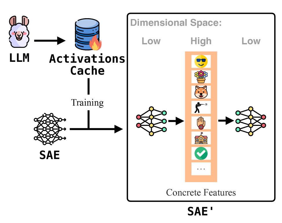
Figure 1: Overview of the sparse autoencoder, illustrating its process for interpreting the internal representations of large language models.

Current SAE training methods primarily focus on base models and follow Block Training paradigm that concatenates datasets and splits them into fixed-length blocks (Joseph Bloom and Chanin, 2024; Bricken et al., 2023). It aligns with the pretraining phase of LLMs, making it a natural and effective choice for training SAEs on base models. While effective for base models, this method faces significant limitations when applied to instruct models (Joseph Bloom and Chanin, 2024; Kissane et al., 2024b). The semantic discontinuity caused by combining data from diverse sources undermines the semantic coherence for alignment with downstream tasks, ultimately degrading SAE training performance (Kissane et al., 2024b).

To address these challenges, we propose Finetuning-aligned Sequential Training (FAST), a novel SAE training method specifically designed for instruct models. FAST processes each data instance independently, preserving semantic integrity and maintaining alignment with the fine-tuning objectives of the model. By providing a consistent and complete semantic space during SAE training, FAST enhances the model’s understanding of input and improves the quality of feature extraction.

Experimental results demonstrate that FAST significantly enhance SAE performance across various tasks. In token reconstruction on Qwen2.5-7B-Instruct (Yang et al., 2024), FAST achieves a mean squared error of 0.6468, outperforming baselines of 5.1985 and 1.5093. It also excels in feature interpretability; for Llama3.2-3B-Instruct (Dubey et al., 2024), 21.1% of features are rated highest in quality, compared to 7.0% for BT(P) and 10.2% for BT(F). Additionally, SAEs are used to study the impact of special tokens on outputs, offering insights into their roles and practical applications, and paving the way for future research.

Our contributions are summarized as follows:

• This paper proposes Finetuning-aligned Sequential Training (FAST), a novel method specifically designed for training SAEs on instruct models.

• Experimental results demonstrate that FAST significantly improves the performance of SAEs on token reconstruction. Additionally, feature interpretability experiments confirm the effectiveness and generalizability of FAST.

• The SAEs are further utilized to investigate the influence of special tokens on model outputs, providing new insights into their specific roles and offering fresh directions for the practical application of SAE models.

2 Related Work

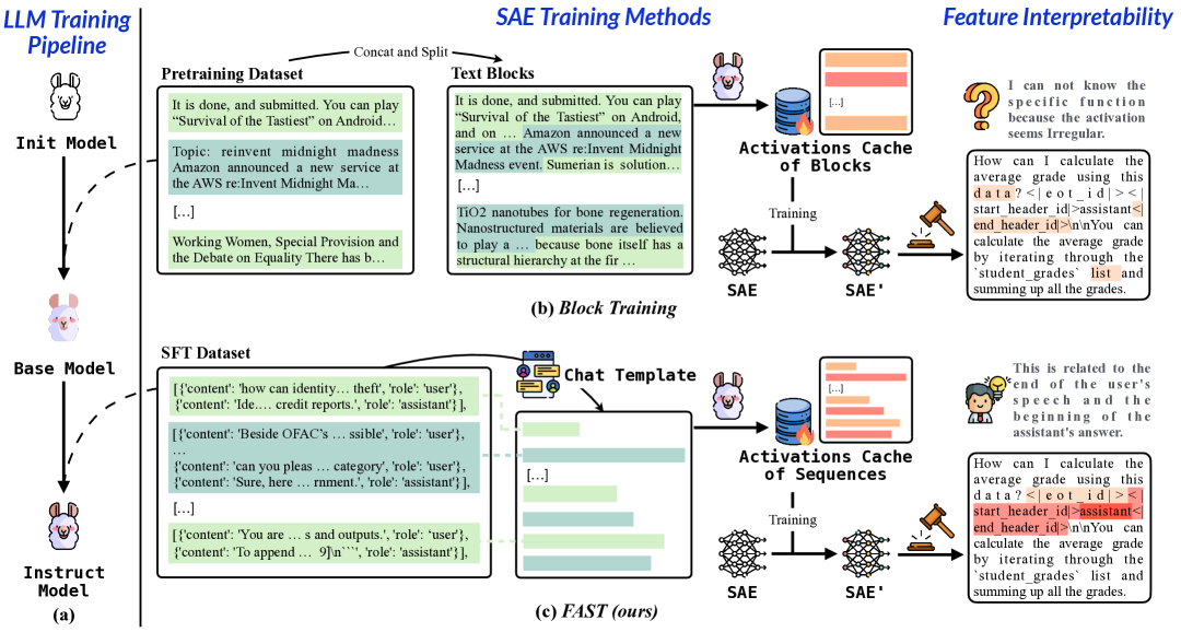
Figure 2: Illustration of the LLM training pipeline and SAE training methods. (a) The pipeline transitions from pretraining to fine-tuning. (b) Block Training (BT) concatenates datasets and resplits them into fixed-length blocks. (c) Finetuning-aligned Sequential Training (FAST) processes data instances independently, preserving semantic integrity and improving alignment with fine-tuning objectives, leading to better performance in feature interpretability.

Mechanistic Interpretability.

As LLMs continue to advance, their increasing complexity, massive parameter scales, and intricate training processes present significant challenges to human understanding of their inner workings (Bubeck et al., 2023; Bengio et al., 2023). Achieving a deep understanding of LLMs is crucial to ensuring alignment with human values (Ji et al., 2023; Anwar et al., 2024) and mitigating harmful or unintended outcomes (Anwar et al., 2024; Hendrycks et al., 2021; Slattery et al., 2024; Hendrycks et al., 2023). However, the "black box" nature (Casper et al., 2024) obscures the underlying causes of misalignment and associated risks. To address these challenges, mechanistic interpretability has emerged as a critical area of research focused on understanding the inner workings of LLMs (Bereska and Gavves, 2024; Nanda, 2022d, 2023, a; Olah, 2022). This discipline seeks to achieve a detailed understanding of model behavior through systematic reverse engineering (Nanda, 2022c, b).

Sparse Autoencoders for LLM.

The training of sparse autoencoders (SAEs) can be framed as a form of dictionary learning, where the hidden layer weights serve as the dictionary basis, and sparsity constraints enforce efficient and sparse data representations (Bereska and Gavves, 2024; Bricken et al., 2023). Additionally, SAEs align with both the linear representations hypothesis (Mikolov et al., 2013) and the superposition hypothesis (Elhage et al., 2022; Arora et al., 2018; Olah et al., 2020), ensuring that the learned representations adhere to theoretical principles of high-dimensional feature spaces. Specifically, the linear representation hypothesis suggests that features in language models correspond to directions in activation space, enabling embedding arithmetic, such as: $v(\text{"king"})-v(\text{"man"})+v(\text{"woman"})=v(\text{"queen"})$ (Mikolov et al., 2013).

Neurons in LLMs are often polysemantic, encoding multiple distinct features due to the limited dimensionality of feature activation space. (Bereska and Gavves, 2024). The superposition hypothesis explains how neural networks represent more features than the number of available neurons by encoding features as nearly orthogonal directions in the neuron output space (Elhage et al., 2022). The activation of one feature may appear as a slight activation of another, resulting from the overlap of non-orthogonal vectors. While such overlaps introduce interference, the advantages of representing a greater number of non-orthogonal features outweigh the drawbacks, particularly in highly sparse neural networks (Bricken et al., 2023; Bereska and Gavves, 2024; Rajamanoharan et al., 2024a). This property makes SAEs particularly valuable in mechanistic interpretability, as they enable the decomposition of language models by capturing high-dimensional features (Gao et al., 2024; Ferrando et al., 2024; Rajamanoharan et al., 2024b; Lieberum et al., 2024; He et al., 2024).

3 Finetuning-aligned Sequential Training

Motivation.

Recent studies have adopted a training paradigm for SAE that builds upon the pretraining phase of LLMs, as illustrated in Figure 2(b). This approach, referred to as Block Training (BT), involves concatenating datasets and splitting them into fixed-length blocks for training (Bereska and Gavves, 2024; He et al., 2024; Kissane et al., 2024a). BT aligns with the pretraining phase of LLMs, making it a natural and effective choice for training SAEs on base models. Since base models are directly trained on large-scale corpora without additional fine-tuning, BT ensures consistency between the SAE training and the pretraining objectives of LLMs.

However, when it comes to instruct models, which undergo a supervised fine-tuning (SFT) phase to align with specific instructions or downstream tasks, the limitations of BT become more apparent. For instance, studies demonstrate that SAE trained on the pretraining dataset exhibit significantly weak abilities in adhering to refusal directives (Kissane et al., 2024b). An alternative approach utilizes SFT datasets, introducing special tokens and applying block training in the same manner (Kissane et al., 2024b). While this method leverages SFT datasets, it still preserves the BT methodology, which does not align well with the finetuning objectives of instruct models. Specifically, BT treats the input sequences as concatenated blocks, often combining data samples from different sources. For example, in a sequence of 8,192 tokens, the first 2,048 tokens may originate from one sample, while the remaining 6,144 tokens come from another. While such semantic discontinuity is less problematic for base models, as it mirrors their pretraining setup, it poses significant challenges for instruct models. Maintaining semantic integrity is crucial for aligning with downstream tasks, and the lack of such alignment hinders the model’s ability to fully understand the input, ultimately degrading SAE training performance.

To address these challenges, we propose a novel SAE training method for instruct models: Finetuning-aligned Sequential Training (FAST), which better aligns with the fine-tuning phase, both in terms of dataset utilization and training methodology in Figure 2(c). By providing the instruct model with a consistent and complete semantic space during SAE training, FAST enhances the alignment with the fine-tuning phase and improves the quality of SAE training. This alignment forms the primary motivation behind FAST.

3.1 Data Processing

As previously described, FAST trains the SAE using finetuning datasets. Specifically, multiple multi-turn dialogue datasets are collected, and each data instance is combined with the corresponding chat template of the instruct model. This process not only introduces special tokens but also ensures consistency with the data processing methodology used during the fine-tuning phase of the model.

A key innovation lies in independent processing of each data instance, rather than concatenating multiple instances before inputting them into the model. By eliminating the constraint of context size, the dataset is processed sequentially. Each data instance is individually fed into the LLM to extract hidden layer activations, which subsequently used to train the SAE, as illustrated in Figure 2(c). This approach effectively avoids semantic discontinuity caused by data concatenation, while preserving the semantic integrity of each instance thereby providing higher-quality inputs for training the SAE.

3.2 SAE

This section introduces the two types of SAE models utilized in FAST: the Standard ReLU-based SAE and the JumpReLU SAE. The Standard ReLU-based SAE is a widely adopted approach (Bereska and Gavves, 2024; Bricken et al., 2023), while JumpReLU SAE achieves superior reconstruction quality and sparsity control (Rajamanoharan et al., 2024a; Lieberum et al., 2024). Here we provide the details of the two SAE models and the initialization method in Appendix A.

Standard SAE.

For the input vector $x\in\mathbb{R}^{d_{in}}$ from the residual stream, $d_{in}$ denotes the dimensionality of the model’s hidden layer. The ReLU-based SAE model consists of an encoder, decoder, and a corresponding loss function, which are defined as follows:

$$f(\mathbf{x}) =\text{ReLU}(\mathbf{W}^{\text{enc}}\mathbf{x}+\mathbf{b}^{\text{enc}})$$ (1)

$$\hat{\mathbf{x}} =\mathbf{W}^{\text{dec}}f(\mathbf{x})+\mathbf{b}^{\text{dec}}$$ (2)

$$\mathcal{L} =\|\mathbf{x}-\hat{\mathbf{x}}\|_{2}^{2}+\lambda\|\mathbf{z_{L1}}\|$$ (3)

$\mathbf{W}^{\text{enc}}$, $\mathbf{W}^{\text{dec}}$, $\mathbf{b}^{\text{enc}}$, $\mathbf{b}^{\text{dec}}$ represent the weight matrices and bias vectors for the encoder and decoder, respectively. $\|\mathbf{x}-\hat{\mathbf{x}}\|_{2}^{2}$ denotes the mean squared error (MSE) loss, $\|\mathbf{z_{L1}}\|_{1}$ represents the $L_{1}$ loss used for sparsity regularization, and $\lambda$ is the sparsity regularization hyperparameter.

JumpReLU SAE.

The JumpReLU SAE retains the same parameter matrices $\mathbf{W}$ and $\mathbf{b}$ as the Standard SAE but introduces a modified activation function and sparsity regularization:

$$f(\mathbf{x}) =\text{JumpReLU}_{\theta}(\mathbf{W}^{\text{enc}}\mathbf{x}+\mathbf{b}^{\text{enc}}),$$ (4)

$$\hat{\mathbf{x}} =\mathbf{W}^{\text{dec}}f(\mathbf{x})+\mathbf{b}^{\text{dec}},$$ (5)

$$\mathcal{L} =\|\mathbf{x}-\hat{\mathbf{x}}\|_{2}^{2}+\lambda\|\mathbf{z_{L0}}\|,$$ (6)

The JumpReLU function is defined as $\text{JumpReLU}_{\theta}(z):=z\odot H(z-\theta)$, where $\theta>0$ is a learnable, vector-valued threshold parameter. Here, $\odot$ denotes elementwise multiplication, and $H$ represents the Heaviside step function. Additionally, $\|\mathbf{z_{L0}}\|_{1}$ represents the $L_{0}$ loss used for sparsity regularization, while $\lambda$ is the sparsity regularization hyperparameter.

3.3 Mixing Activation Buffer

Activation values, which represent the activation levels of hidden layer dimensions during the model’s forward pass, require significant storage space. To mitigate this challenge, we employ a producer-consumer framework inspired by previous studies (Joseph Bloom and Chanin, 2024), wherein the LLM generates activations and stores them in a dedicated buffer.

As shown in Figure 3, the process begins with the buffer being filled to capacity with activation values. Once the buffer is full, the activations are shuffled to ensure randomness and diversity. Subsequently, half of the shuffled activations are sent to the SAE model for training, while the other half remains in the buffer. After training, the buffer is replenished with new activations generated by the model, and the cycle repeats. This iterative mechanism optimizes storage efficiency and ensures a high level of data variability, thereby enhancing the robustness of model training. By leveraging the mixing buffer, this approach effectively balances data diversity with storage efficiency.

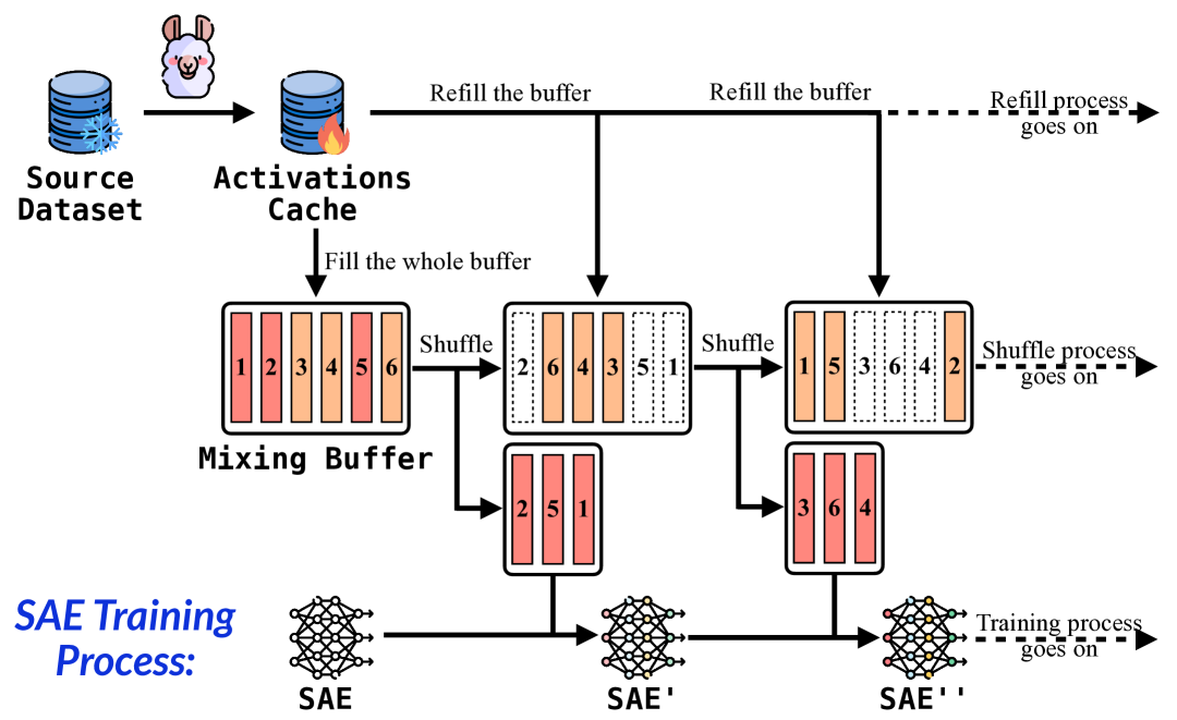
Figure 3: The mixing activation buffer is shuffled, half is sent to the SAE for training, and the resulting new activations are used to refill the buffer. This iterative process ensures data diversity and storage efficiency.

4 Experiments

4.1 Experiment Setup

Dataset.

We construct a large-scale instruction dataset for fine-tuning LLMs by combining several publicly available, high-quality datasets, including WildChat-1M-Full (Zhao et al., 2024), Infinity-Instruct (BAAI, 2024), tulu-3-sft-mixture (Lambert et al., 2024), orca-agentinstruct-1M-v1-cleaned , and lmsys-chat-1m (Zheng et al., 2023). After applying a 20-gram deduplication strategy, it is reduced to 4,758,226 samples. Details are in Appendix B.

LLMs.

We conduct experiments on seven models from two families: Llama (Llama-3.1, Llama-3.2)(Dubey et al., 2024) and Qwen (Qwen-2.5)(Yang et al., 2024), selected for their state-of-the-art performance to evaluate our approach’s robustness and generalization across families and scales. The models and their respective layer configurations, detailed in Table 1, are selected from various depths to mitigate depth bias. Following prior works (Bereska and Gavves, 2024; Bricken et al., 2023; Gao et al., 2024), we train SAEs on the residual stream, as inter-layer relationships have minimal impact on performance.

Baselines.

Prior to this study, all SAE model training methods exclusively utilize the Block Training (BT) strategy. Depending on the type of training dataset used, Block Training can be categorized into two primary forms: BT(P) and BT(F) as follows:

• BT(P): Block Training using the pretraining dataset. The pretraining dataset is processed by concatenating and segmenting the data into text blocks of equal length, which are then used for training the SAE model.

• BT(F): Block Training using the finetuning dataset. This approach utilizes a finetuning dataset. The data within the dataset is concatenated to form text blocks.

For BT(P), we utilize the pile-uncopyrighted dataset . As for BT(F), we use the finetuning dataset metioned before which is also used in FAST.

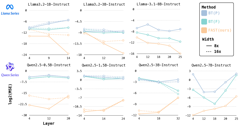
Figure 4: $\mathrm{MSE}_{st}$ performance of the JumpReLU SAE (all metrics are presented in log scale, where lower values indicate better SAE reconstruction performance). Within the JumpReLU architecture, FAST exhibits the best reconstruction capability compared to BT(P) and BT(F).

Configuration.

SAEs are trained on 8*NVIDIA A100 GPUs using sae_lens (Joseph Bloom and Chanin, 2024) with custom implementation. For models more than 7B parameters, the expansion factor of SAE is fixed at 8X, whereas for other models, the expansion factor can be 8X or 16X. To ensure fairness across methods at the same data scale, the number of training tokens is set to 40,960,000. For BT(P) and BT(F), context_size is 2,048, with each text block containing 2,048 tokens. For FAST, no explicit context_size is required; instead, a truncation length of 8,192 is applied to manage memory usage. For JumpReLU SAE, $L_{\text{sparsity}}$ is 0.01, while for Standard SAE, it is 5. Further parameter details are in Appendix C.

Model Name	Layer
Llama series
Llama-3.1-8B-Instruct	[4,12,18,20,25]
Llama-3.2-3B-Instruct	[4,12,20]
Llama-3.2-1B-Instruct	[4,9,14]
Qwen series
Qwen2.5-7B-Instruct	[4,12,18,20,25]
Qwen2.5-3B-Instruct	[4,18,32]
Qwen2.5-1.5B-Instruct	[4,14,24]
Qwen2.5-0.5B-Instruct	[4,12,20]

Table 1: Layer configurations of the Llama and Qwen model series, showcasing the selection of layers across varying depths to mitigate depth-related biases and optimize model performance.

Evaluation Metric.

The performance of the SAE is assessed using the Mean Squared Error ($\mathrm{MSE}$), which is calculated as:

$$\mathrm{MSE}=\frac{\sum_{i=1}^{N}\frac{1}{L_{i}}\sum_{j=1}^{L_{i}}\sum_{k=1}^{H}(y_{i,j,k}-\hat{y}_{i,j,k})^{2}}{N\cdot H}$$ (7)

where $N$ denotes the size of the dataset, $L_{i}$ represents the length of the $i$-th sequence, $H$ refers to the hidden dimension of the model. To evaluate the SAE’s performance specifically on special tokens, we also compute the MSE of special tokens, denoted as $\mathrm{MSE}_{st}$. Lower $\mathrm{MSE}$ values reflect better model performance.

4.2 Main Results

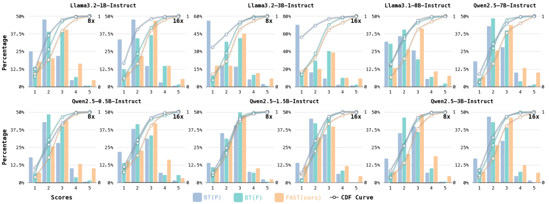
Figure 5: Experiment results of feature interpretability.FAST achieves notable improvements compared to the other two training methods across all the tested models. FAST attains 21.1% of features rated in the highest quality range (scores 4-5), in contrast to 7.0% for BT(P) and 10.2% for BT(F).

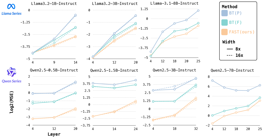
Figure 6: $\mathrm{MSE}_{st}$ performance of the Standard SAE (all metrics are presented in log scale, where lower values indicate better SAE reconstruction performance). Within the Standard architecture, FAST exhibits the best reconstruction capability compared to BT(P) and BT(F)

A random sample of 5,000 dialogues is extracted from the remaining portion of the dataset for evaluation. Figure 4 compares the $\mathrm{MSE}_{st}$ scores of three methods using the JumpReLU SAE, while Figure 6 illustrates the $\mathrm{MSE}_{st}$ performance of the Standard SAE. Detailed results for both $\mathrm{MSE}$ and $\mathrm{MSE}_{st}$ are presented in Appendix D.

In terms of overall token reconstruction ($\mathrm{MSE}$), the JumpReLU architecture with Qwen models demonstrates similar patterns, with FAST consistently outperforming baseline methods. FAST method achieves superior performance across most configurations. For instance, in Llama-3.2-3B-Instruct-L20-8X-Standard, FAST attains -0.9527, significantly surpassing the baselines which score -0.6926 and -0.9186. In special token reconstruction ($\mathrm{MSE}_{st}$), FAST shows marked improvements across models. In Qwen2.5-7B-Instruct-L18-8X-Standard, FAST achieves 0.6468, outperforming the baselines (5.1985 and 1.5093). In the JumpReLU SAEs, it achieves -9.7604 compared to -4.0005 and -8.0743.

Overall, the findings demonstrate that FAST excels in reconstructing both general and special tokens. Interestingly, FAST shows even stronger improvements in Standard SAE architectures compared to JumpReLU SAEs, potentially due to the latter’s already high $\mathrm{MSE}$ performance, leaving less room for enhancement. Despite limitations in Standard architectures due to L1 regularization and ReLU activation, FAST significantly improves token reconstruction in these models.

5 Feature Interpretability

Score	Description
5	Clear pattern with no deviating examples
4	Clear pattern with one or two deviating examples
3	Clear overall pattern but quite a few examples not fitting that pattern
2	Broad consistent theme but lacking structure
1	No discernible pattern

Table 2: Scoring criteria for feature interpretability.

This section evaluates the interpretability of features extracted by SAEs through an automated analysis framework, building upon methodologies (Bills et al., 2023; Cunningham and Conerly, 2024; He et al., 2024). The middle layers of the trained SAEs are selected for analysis based on their demonstrated superior performance. Given that experiments demonstrate that the JumpReLU activation function outperforms other alternatives (Rajamanoharan et al., 2024b; Lieberum et al., 2024), the evaluation exclusively employs SAEs equipped with JumpReLU. Table 10 presents the specific SAE models evaluated.

Additional 10,000 instances are sampled and their activation values are computed. Then the top five sentences with the highest activation values are identified to construct an activation dataset for evaluating features. Based on the assumption that dead features are irrelevant to the evaluation, an initial screening of features is conducted, ensuring that only features with non-zero activation values in top five sentences are retained. After that, we randomly select 128 features as the final evaluation.

GPT-4o is prompted to score each group of five contexts and generate a descriptive summary. Additionally, a monosemanticity score ranging from 1 to 5 is assigned, based on a rubric adapted from  (Cunningham and Conerly, 2024; He et al., 2024). Detailed prompt is shown in Appendix E.2.

A total of 4,608 feature scores are computed and presented in Figure 5. The results demonstrate that FAST consistently outperforms BT(P) and BT(F) across all evaluated SAEs. For the 8x scaled Llama3.2-3B-Instruct, FAST achieves 21.1% of features in the highest quality range (scores 4-5), compared to 7.0% for BT(P) and 10.2% for BT(F). Generally, compared to both baseline methods, we observe that FAST reduces the proportion of low-quality features while increasing the proportion of high-quality features in 8X and 16X SAEs. This highlights the superiority of FAST in producing more interpretable features during SAE training.

Furthermore, Cumulative Distribution Function (CDF) curve analysis reveals that FAST’s percentage of features scoring below 3 is consistently the lowest. For instance, with Qwen2.5-3B-Instruct model, the CDF at score 3 is 76.5% for FAST, compared to 89.0% for BT(F) and 92.2% for BT(P), indicating fewer low-scoring features for FAST. These findings suggest that both appropriate training dataset selection for SAEs and the sequence training methodology contribute to enhanced model interpretability. FAST appears to successfully integrate these aspects, leading to more interpretable SAEs.

6 Steering with SAE Latents

Feature steering represents an intuitive approach to evaluate model inference by adjusting the activation coefficients within a trained SAE, thereby directly influencing the model’s output. This method resembles the use of decoder latent vectors for activation guidance, but the SAE offers a more robust and unambiguous process for activation guidance. Based on the formulations in Equations 2 and 5, the reconstructed outputs of the SAE derive from a weighted combination of its latent variables. (Ferrando et al., 2024; Templeton, 2024).

$$z^{\prime}=z+\alpha d_{k}$$ (8)

These latent variables correspond to row vectors of $W_{\text{dec}}$, with $\alpha$ scaling the $k$-th latent. To implement this steering, a latent dimension $k$ is selected, scaling its decoder vector $d_{k}$ by $\alpha$. Then $z^{\prime}$ is introduced into the model’s residual stream.

Following  Ferrando et al. (2024), 1,010 sampled instruction instances are randomly partitioned into two parts: 1,000 samples to identify highly activated SAE features and 10 samples to evaluate post-steering model outputs. We use the chat template corresponding to the instruct model during inference. The 10 questions appear in Appendix F.1. We focus on feature related to these special tokens(shown in Table 11) to examine how special tokens, which are not associated with specific entities, influence the model’s output. Using 1,000 samples, the average maximum activation values are calculated for each feature. Complete activation values for each model appear in Appendix F.3.

Three representative questions are selected to illustrate the effects of steering features. Due to space constraints, feature steering primarily focuses on the <|start_header_id|> for Llama3.1-8B-Instruct and <|im_start|> for Qwen2.5-7B-Instruct. The experiments employ scaling $\alpha\in[0,15,25,50,100,150,200]$ using 8X JumpReLU SAE through FAST and greedy decoding. Detailed analyses of three questions are presented in Appendix F.4.

Steering high-activation features particularly those associated with special tokens significantly influences the model’s output quality and reasoning ability. This effect remains consistent across diverse tasks and linguistic contexts. There is an optimal range for the coefficient $\alpha$. Within this range, model responses become more accurate, coherent, and relevant to the given instructions.

For instance, in Question 3(F.4.2), amplifying the activation of a feature tied to both the <|im_start|> and user results in a clear transition: moderate values of $\alpha$ improved engagement and output relevance, while excessive amplification led to language switching and incoherent, repetitive text. Similarly, in Question 4(F.4.3), steering the highest activation feature associated with the <|im_start|> marker within a specific coefficient range led to more convincing and logically structured answers, but pushing $\alpha$ too far again degraded output quality. Similar patterns can also be observed in Q2(F.4.1).

The consistency in findings suggests that these features encode essential aspects of the model’s reasoning capabilities, transcending individual tasks or linguistic contexts. There is an optimal coefficient $\alpha$ range suggests a "sweet spot" for feature steering, enhancing performance without introducing the degradation seen at higher coefficients.

This observation presents important implications for the practical application of SAEs. It demonstrates that steering certain features potentially associated with special tokens emerges as a reliable method to improve model performance across diverse tasks. Unlike traditional SAE-feature approaches, which often impose output biases tied to predefined meanings or entities, feature steering with special tokens refines the guidance of models, resulting in higher-quality responses.

7 Conclusion

This paper proposes a novel approach, Finetuning-aligned Sequential Training (FAST), for training SAEs on instruct models. By independently processing individual data instances while maintaining semantic integrity, FAST addresses the limitations of traditional Block Training (BT) methods, which often suffer from semantic discontinuity and misalignment with downstream task requirements. Experimental results show that FAST improves performance across various SAE models, demonstrating its versatility and general applicability. Furthermore, FAST consistently achieves superior results in feature interpretability evaluations, highlighting its effectiveness and advantages.

Also we employ SAEs to explore the influence of special tokens on model outputs. Results indicate that steering features within a specific coefficient range substantially enhance model output quality. These insights provide a valuable method for studying the functional roles of special tokens and practical applications of SAEs. To facilitate future research, the complete codebase, datasets and a total of 240 pre-trained SAE models will be released publicly, establishing a robust foundation for innovation and advancement in this domain.

Limitations

As language models increase in scale, investigating their internals with SAE-based methods becomes more challenging. Computational constraints restrict our investigation to smaller Qwen and Llama models (under 8B parameters), though our framework could be extended to larger architectures. Feature interpretability analysis focuses mainly on strongly activated features, potentially overlooking weakly activated samples (He et al., 2024). Furthermore, feature steering experiments are preliminary studies centered on special token-related features that correlate with response quality. A more comprehensive investigation of these features’ influence remains an important direction for future research.

Ethical Statements

This research focuses on interpreting and steering instruction-tuned language models through sparse autoencoders. All experiments rely solely on publicly available, appropriately licensed text corpora that are deduplicated and stripped of personally identifiable information; no human subjects are involved nor private data collected. Nevertheless, it is important to acknowledge that LLMs are trained on extensive publicly available datasets, potentially resulting in inadvertent reproduction of copyrighted material. Our codes, parameters, and deduplicated demo data will be released under an open-source licence to support reproducibility.

Appendix A SAE Initialization Method

The encoder weights ($W_{enc}$) and decoder weights ($W_{dec}$) are initialized using the Kaiming Uniform initialization method (He et al., 2015). This step, used exclusively in the JumpReLU method, normalizes each row of the $W_{dec}$ using the L2 norm and adjusts the threshold $\epsilon$ and encoder bias $b_{enc}$ accordingly. After that, some data is selected for geometric median evaluation. The goal is to minimize the weighted sum of distances to all sample points. To achieve this, the Weiszfeld algorithm is employed to a specified precision of $\text{ftol}=1\times 10^{-20}$. The resulting optimal point is then used as the initial value for $b_{\text{dec}}$, which is set to 0. There exists the formulas about the geometric median evaluation as follows:

$$f(\mathbf{m})=\sum_{i=1}^{n}w_{i}\|\mathbf{m}-\mathbf{p}_{i}\|,\mathbf{m}_{0}=\frac{\sum_{i=1}^{n}w_{i}\mathbf{p}_{i}}{\sum_{i=1}^{n}w_{i}}$$ (9)

$$d_{i}=\|\mathbf{p}_{i}-\mathbf{m}_{k}\|,w_{i}^{\prime}=\frac{w_{i}}{\max(d_{i},\epsilon)}$$ (10)

$$\mathbf{m}_{k+1}=\frac{\sum_{i=1}^{n}w_{i}^{\prime}\mathbf{p}_{i}}{\sum_{i=1}^{n}w_{i}^{\prime}}$$ (11)

$$\left|f(\mathbf{m}_{k+1})-f(\mathbf{m}_{k})\right|\leq\text{ftol}\cdot f(\mathbf{m}_{k})$$ (12)

The parameters used in the equations are defined as follows: $\mathbf{m}$ represents the target point or the weighted mean to be optimized, while $\mathbf{p}_{i}$ is the $i$-th data point in the dataset. $w_{i}$ denotes the weight associated with the $i$-th data point. The objective function, $f(\mathbf{m})$, is the weighted sum of distances between $\mathbf{m}$ and all data points $\mathbf{p}_{i}$. The initial estimate of $\mathbf{m}$, denoted as $\mathbf{m}_{0}$, is calculated as the weighted mean of all points. $d_{i}$ is the distance between the $i$-th data point $\mathbf{p}_{i}$ and the current estimate $\mathbf{m}_{k}$. The updated weight for the $i$-th data point, $w_{i}^{\prime}$, is adjusted by the distance $d_{i}$ and a small constant $\epsilon$ to prevent division by zero. $\mathbf{m}_{k+1}$ is the updated estimate of $\mathbf{m}$ at iteration $k+1$, computed as the weighted mean of all points using the updated weights $w_{i}^{\prime}$.

Appendix B SFT Dataset Construction Details

We collect and integrate several large-scale instruction datasets specifically designed for fine-tuning LLMs. Datasets are shown below:

• WildChat-1M-Full (Zhao et al., 2024) is a dataset comprising 1 million conversations between human users and ChatGPT, enriched with demographic metadata such as state, country, hashed IP addresses, and request headers.

• Infinity-Instruct (BAAI, 2024) is a large-scale, high-quality instruction dataset, specifically designed to enhance the instruction-following capabilities of LLMs in both general and domain-specific tasks.

• tulu-3-sft-mixture (Lambert et al., 2024) is used to train the Tulu 3 series of models

• orca-agentinstruct-1M-v1-cleaned  is a cleaned version of the orca-agentinstruct-1M-v1 (Mitra et al., 2024) dataset released by Microsoft, a fully synthetic dataset using only raw text publicly available on the web as seed data.

• lmsys-chat-1m (Zheng et al., 2023) is a comprehensive real-world conversational dataset containing one million interactions with 25 LLMs. This dataset spans a wide range of topics and interaction types, effectively capturing diverse user-LLM interaction patterns.

Together, they comprise 11,425,231 samples, forming a robust and diverse foundation for advancing research on instruct LLMs. Inevitably, many datasets contain a significant amount of similar or even duplicate data, which can adversely affect both model training and the accuracy of evaluations. To address this issue, we employ an n-gram-based deduplication technique to preprocess the data (Algorithm 1). N-gram method decomposes text into consecutive sequences of n words (or characters), effectively capturing local features.

Algorithm 1 Deduplicate Dataset by N-Grams

0: Dataset $\mathcal{D}$, N-gram size $n$

0: Deduplicated dataset $\mathcal{D}_{dedup}$

1: $\mathcal{D}_{dedup}\leftarrow\{\}$ # Initialize deduplicated dataset

2: $seen\_hashes\leftarrow\{\}$ # Set to store hashes of seen N-grams

3: for each sample $s$ in $\mathcal{D}$ do

4:  $ngrams\leftarrow\{\}$ # Initialize N-grams for the sample

5:  for each conversation $c$ in $s.conversations$ do

6:   $ngrams\leftarrow ngrams\cup\mathrm{GenerateNGrams}(c.content,n)$

7:  end for

8:  if $\mathrm{any}$ $\mathrm{Hash}(ngram)\in seen\_hashes$ for $ngram\in ngrams$ then

9:   continue #Skip sample if any N-gram hash is already seen

10:  end if

11:  $seen\_hashes\leftarrow seen\_hashes\cup\{\textbf{Hash}(ngram)\mid ngram\in ngrams\}$

12:  $\mathcal{D}_{dedup}\leftarrow\mathcal{D}_{dedup}\cup\{s\}$

13: end for

14: return  $\mathcal{D}_{dedup}$

This approach enables the detection and identification of repetitive patterns within the text. By leveraging this method, we are able to filter out not only completely identical instances but also content that exhibits high semantic or structural similarity. Consequently, the quality and diversity of the dataset are significantly enhanced. Finally, we adopt a 20-gram deduplication strategy to eliminate redundancy in the dataset. After applying this process, a total of 4,758,226 data entries are obtained.

Appendix C Hyperparameter Settings

The detailed parameter settings used in the experiment are as follows:

General Settings

• Learning Rate ($lr$): $7\times 10^{-5}$

• End Learning Rate ($lr_{end}$): $7\times 10^{-6}$

• Seed: $42$

• Data Type ($dtype$): float32

Optimizer Settings

• Optimizer: Adam

  • Beta 1 ($\beta_{1}$): $0.9$

  • Beta 2 ($\beta_{2}$): $0.999$

• Learning Rate Scheduler: cosineannealing

  • Learning Rate Decay Steps: $64,000$

  • Learning Rate Warm-up Steps: $16,000$

• Sparsity Loss Coefficient ($L_{\text{sparsity}}$):

  • $0.01$ for JumpReLU

  • $5$ for Standard

• Sparsity Loss Warm-up Steps ($L_{\text{sparsity}}$): $10,000$

Training Settings

• Training Tokens: $4.096\times 10^{7}$

• Train Batch Size (tokens): $128$

Activation and Decoder Initialization

• Decoder Initialization Method ($b_{dec\_init\_method}$): geometric_median

• Normalize SAE Decoder: True

• Dead Feature Threshold: $10^{-8}$

• Dead Feature Window: $1000$

Additional Settings

• Noise Scale: $0$

• Expansion Factor: $8$ or $16$

• Feature Sampling Window: $2000$

• JumpReLU Bandwidth: $0.001$

• JumpReLU Init Threshold: $0.001$

• Apply Decoder to Input ($apply\_b\_dec\_to\_input$): False

• Use Ghost Gradients: False

• Use Cached Activations: False

Appendix D Mean Squared Error (MSE) of SAEs

The Mean Squared Error (MSE) results for the token reconstruction task are presented in this section.

D.1 Mean Squared Error (MSE) of special tokens of standard SAEs

While the reconstruction capability of Standard SAE models was generally inferior to the JumpReLU structure, FAST is also able to effectively reduce the $\mathrm{MSE}_{st}$, especially in the Qwen series models.

D.2 MSE of SAEs trained on Llama-3.1-8B-Instruct

Layer	Expansion	Method	Standard SAE		JumpReLU SAE
	Factor		$\log_{2}(\mathrm{MSE})$	$\log_{2}(\mathrm{MSE}_{st})$	$\log_{2}(\mathrm{MSE})$	$\log_{2}(\mathrm{MSE}_{st})$
4	8	BT(P)	-5.5059	-4.2377	-9.4350	-6.8026
		BT(F)	-5.6080	-4.8046	-9.8097	-8.3853
		FAST	-5.6432	-4.7236	-9.8187	-10.1534
12	8	BT(P)	-3.2837	-1.6776	-11.2353	-5.4823
		BT(F)	-3.3437	-2.8733	-13.9975	-9.2049
		FAST	-3.4104	-3.0011	-14.1393	-12.1287
18	8	BT(P)	-1.6059	-0.6085	-13.0282	-7.4267
		BT(F)	-1.7131	-1.6009	-15.0851	-10.4278
		FAST	-1.8697	-2.2923	-15.0666	-12.4442
20	8	BT(P)	-1.1852	-0.1692	-13.3080	-7.8271
		BT(F)	-1.3509	-1.3587	-14.7969	-10.4507
		FAST	-1.4721	-1.9375	-15.5552	-13.1463
25	8	BT(P)	-0.1677	1.0444	-12.9767	-7.1657
		BT(F)	-0.5163	-0.5639	-16.6192	-11.6569
		FAST	-0.5747	-0.8982	-16.5138	-15.9845

Table 3: Mean Squared Error (MSE) of SAEs trained on Llama-3.1-8B-Instruct. Each value is highlighted with a green background to indicate performance, with darker shades of green representing better results.

D.3 MSE of SAEs trained on Llama-3.2-3B-Instruct

Layer	Expansion	Method	Standard SAE		JumpReLU SAE
	Factor		$\log_{2}(\mathrm{MSE})$	$\log_{2}(\mathrm{MSE}_{st})$	$\log_{2}(\mathrm{MSE})$	$\log_{2}(\mathrm{MSE}_{st})$
4	8	BT(P)	-4.5650	-3.8363	-13.7434	-8.3908
		BT(F)	-4.5785	-3.8250	-13.6105	-8.5868
		FAST	-4.5931	-3.9053	-9.0852	-8.7193
	16	BT(P)	-4.5645	-3.8158	-9.6278	-7.5321
		BT(F)	-4.5858	-3.8210	-9.6102	-7.6905
		FAST	-4.5959	-3.9055	-9.8054	-9.3065
12	8	BT(P)	-2.6239	-1.9052	-13.4038	-8.5246
		BT(F)	-2.6757	-2.1318	-14.7879	-9.1440
		FAST	-2.7236	-2.4763	-15.3747	-13.4614
	16	BT(P)	-2.6279	-1.9488	-12.2827	-7.7836
		BT(F)	-2.6754	-2.2725	-13.8874	-8.4299
		FAST	-2.7509	-2.5644	-14.4420	-12.6355
20	8	BT(P)	-0.6926	-0.4378	-13.5554	-8.4006
		BT(F)	-0.9186	-1.0709	-14.8424	-8.9061
		FAST	-0.9527	-1.4473	-18.8809	-17.3707
	16	BT(P)	-0.8145	-0.4607	-13.1516	-9.1137
		BT(F)	-1.0947	-1.1447	-14.2900	-8.9611
		FAST	-1.1285	-1.5387	-14.6872	-12.1711

Table 4: Mean Squared Error (MSE) of SAEs trained on Llama-3.2-3B-Instruct. Each value is highlighted with a green background to indicate performance, with darker shades of green representing better results.

D.4 MSE of SAEs trained on Llama-3.2-1B-Instruct

Layer	Expansion	Method	Standard SAE		JumpReLU SAE
	Factor		$\log_{2}(\mathrm{MSE})$	$\log_{2}(\mathrm{MSE}_{st})$	$\log_{2}(\mathrm{MSE})$	$\log_{2}(\mathrm{MSE}_{st})$
4	8	BT(P)	-5.3374	-4.4021	-15.3160	-9.6296
		BT(F)	-5.3583	-4.4375	-15.6237	-10.0324
		FAST	-5.3775	-4.3920	-15.8654	-13.9127
	16	BT(P)	-5.3370	-4.3794	-14.5574	-9.0583
		BT(F)	-5.3587	-4.4358	-14.7275	-9.4817
		FAST	-5.3804	-4.3879	-10.5009	-10.2448
9	8	BT(P)	-3.6638	-2.9507	-7.9900	-7.2577
		BT(F)	-3.7759	-3.0874	-16.1021	-10.5349
		FAST	-3.8282	-3.5754	-16.4928	-13.9685
	16	BT(P)	-3.6642	-2.9456	-7.1584	-6.5155
		BT(F)	-3.8049	-3.3775	-15.1966	-9.8149
		FAST	-3.8344	-3.6778	-15.8696	-12.9629
14	8	BT(P)	-1.2195	-0.4927	-8.0419	-5.1825
		BT(F)	-1.7311	-1.7559	-15.2996	-9.3409
		FAST	-1.7410	-2.6844	-21.4449	-23.4395
	16	BT(P)	-1.2449	-0.5642	-6.4784	-5.2817
		BT(F)	-1.8371	-1.8036	-14.9445	-9.3654
		FAST	-1.8409	-2.7668	-16.2748	-13.3547

Table 5: Mean Squared Error (MSE) of SAEs trained on Llama-3.2-1B-Instruct. Each value is highlighted with a green background to indicate performance, with darker shades of green representing better results.

D.5 MSE of SAEs trained on Qwen2.5-7B-Instruct

Layer	Expansion	Method	Standard SAE		JumpReLU SAE
	Factor		$\log_{2}(\mathrm{MSE})$	$\log_{2}(\mathrm{MSE}_{st})$	$\log_{2}(\mathrm{MSE})$	$\log_{2}(\mathrm{MSE}_{st})$
4	8	BT(P)	1.2919	7.2207	-4.1852	1.9109
		BT(F)	-0.5233	0.0494	-5.9622	-3.3368
		FAST	-0.7358	-1.6090	-10.6174	-11.9105
12	8	BT(P)	1.4751	5.7788	-5.8014	-4.1171
		BT(F)	0.7681	0.9550	-6.3039	-5.9309
		FAST	0.6177	-0.0770	-9.8207	-10.4545
18	8	BT(P)	2.0024	5.1985	-6.5926	-4.0005
		BT(F)	1.4749	1.5093	-6.8466	-8.0743
		FAST	1.3892	0.6468	-9.1659	-9.7604
20	8	BT(P)	2.6772	5.1501	-4.9649	-0.7776
		BT(F)	2.1453	1.9877	-5.6461	-3.5904
		FAST	2.0796	1.1869	-8.2213	-8.7821
25	8	BT(P)	4.8764	6.2532	-2.1482	2.0938
		BT(F)	4.4139	3.7031	-2.6957	1.6207
		FAST	4.4471	3.0934	-4.9598	-5.5615

Table 6: Mean Squared Error (MSE) of SAEs trained on Qwen2.5-7B-Instruct. Each value is highlighted with a green background to indicate performance, with darker shades of green representing better results.

D.6 MSE of SAEs trained on Qwen2.5-3B-Instruct

Layer	Expansion	Method	Standard SAE		JumpReLU SAE
	Factor		$\log_{2}(\mathrm{MSE})$	$\log_{2}(\mathrm{MSE}_{st})$	$\log_{2}(\mathrm{MSE})$	$\log_{2}(\mathrm{MSE}_{st})$
4	8	BT(P)	-0.8873	2.8616	-8.7177	-2.2147
		BT(F)	-1.4572	1.1595	-8.5340	-1.9954
		FAST	-1.5098	-1.6682	-13.9907	-11.6534
	16	BT(P)	-1.0058	2.8627	-8.8511	-2.3755
		BT(F)	-1.6685	1.1371	-8.9769	-2.4576
		FAST	-1.5147	-1.7482	-13.2162	-10.7660
18	8	BT(P)	0.9257	3.0243	-9.2313	-2.9916
		BT(F)	0.4744	1.1862	-9.3796	-2.9188
		FAST	0.6782	-0.9288	-10.3007	-11.2916
	16	BT(P)	0.8594	3.4799	-9.6147	-3.1930
		BT(F)	0.3438	1.1729	-9.5534	-3.0426
		FAST	0.5485	-1.0730	-10.3197	-11.1114
32	8	BT(P)	3.8883	4.7227	-4.3442	-2.3480
		BT(F)	3.4388	3.7056	-5.5300	-5.3856
		FAST	3.6647	1.6953	-5.0278	-7.3022
	16	BT(P)	3.7736	4.6584	-4.4299	-2.9327
		BT(F)	3.2978	3.4334	-5.6515	-6.2729
		FAST	3.5676	1.4331	-5.0783	-7.2653

Table 7: Mean Squared Error (MSE) of SAEs trained on Qwen2.5-3B-Instruct. Each value is highlighted with a green background to indicate performance, with darker shades of green representing better results.

D.6.1 Qwen2.5-1.5B-Instruct

Layer	Expansion	Method	Standard SAE		JumpReLU SAE
	Factor		$\log_{2}(\mathrm{MSE})$	$\log_{2}(\mathrm{MSE}_{st})$	$\log_{2}(\mathrm{MSE})$	$\log_{2}(\mathrm{MSE}_{st})$
4	8	BT(P)	-0.1150	3.8222	-5.0404	1.5111
		BT(F)	-0.5653	3.2719	-5.1794	1.3737
		FAST	-0.7745	-2.1358	-13.4069	-12.5193
	16	BT(P)	-0.2315	3.8196	-4.8980	1.6550
		BT(F)	-0.7614	3.2068	-5.1495	1.4045
		FAST	-0.9958	-2.0996	-13.3622	-11.6841
14	8	BT(P)	0.4087	3.5463	-5.4990	1.0522
		BT(F)	0.0306	2.9569	-6.2791	0.2762
		FAST	-0.0925	-1.2535	-11.2579	-11.8198
	16	BT(P)	0.3186	3.5454	-4.9561	1.5981
		BT(F)	-0.0918	3.0073	-5.9567	0.5989
		FAST	-0.2312	-1.3543	-11.6309	-12.1911
24	8	BT(P)	3.0506	4.3907	-4.6425	0.4759
		BT(F)	2.5424	3.5608	-5.3630	0.5141
		FAST	2.5122	0.6336	-6.2603	-7.9484
	16	BT(P)	2.9411	4.3725	-4.4566	1.1218
		BT(F)	2.3877	3.5499	-5.0298	1.0916
		FAST	2.3762	0.3794	-6.3063	-8.0686

Table 8: Mean Squared Error (MSE) of SAEs trained on Qwen2.5-1.5B-Instruct. Each value is highlighted with a green background to indicate performance, with darker shades of green representing better results.

D.7 MSE of SAEs trained on Qwen2.5-0.5B-Instruct

Layer	Expansion	Method	Standard SAE		JumpReLU SAE
	Factor		$\log_{2}(\mathrm{MSE})$	$\log_{2}(\mathrm{MSE}_{st})$	$\log_{2}(\mathrm{MSE})$	$\log_{2}(\mathrm{MSE}_{st})$
4	8	BT(P)	-2.7554	-0.1257	-10.6725	-4.1202
		BT(F)	-2.8808	-1.3213	-11.6763	-5.1212
		FAST	-2.8732	-3.2218	-21.7343	-23.1697
	16	BT(P)	-2.9204	-0.0721	-10.7024	-4.1569
		BT(F)	-3.1034	-1.1148	-11.6959	-5.1497
		FAST	-3.0970	-3.2153	-17.4590	-16.7389
12	8	BT(P)	-2.0463	-0.0492	-9.5392	-2.9978
		BT(F)	-2.2811	-1.1008	-10.4276	-3.8743
		FAST	-2.2836	-3.0505	-21.1734	-25.6605
	16	BT(P)	-2.1648	-0.0915	-9.4019	-2.8551
		BT(F)	-2.4489	-1.1418	-10.5582	-4.0043
		FAST	-2.4406	-3.0602	-20.7499	-19.0931
20	8	BT(P)	0.2408	1.3303	-10.5099	-4.2017
		BT(F)	-0.3029	-0.0174	-11.4078	-4.8666
		FAST	-0.3387	-1.9461	-15.2442	-16.9599
	16	BT(P)	0.1296	1.2181	-10.6728	-4.2739
		BT(F)	-0.4536	-0.0825	-11.3337	-4.7864
		FAST	-0.4924	-2.1033	-16.3662	-18.0564

Table 9: Mean Squared Error (MSE) of SAEs trained on Qwen2.5-0.5B-Instruct. The best and second-best methods are highlighted with dark green and light green backgrounds, respectively.

Appendix E Implementation Details of Feature Interpretability

This section provides a detailed explanation of the implementation process for evaluating and interpreting feature interpretability.

E.1 SAEs for Feature Interpretability

Model Name	Layer	Expansion Factor
Llama series
Llama-3.1-8B-Instruct	18	8X
Llama-3.2-3B-Instruct	12	8X&16X
Llama-3.2-1B-Instruct	9	8X&16X
Qwen series
Qwen2.5-7B-Instruct	18	8X
Qwen2.5-3B-Instruct	18	8X&16X
Qwen2.5-1.5B-Instruct	14	8X&16X
Qwen2.5-0.5B-Instruct	12	8X&16X

Table 10: Model configurations of the Llama and Qwen model series.

E.2 Prompt for Feature Interpretability

Appendix F Implementation Details of Steering with SAE Latents

F.1 10 Questions

F.2 Special Tokens

Token ID	Token
Llama series
882	user
78191	assistant
128006	<|start_header_id|>
128007	<|end_header_id|>
128009	<|eot_id|>
Qwen series
872	user
77091	assistant
151644	<|im_start|>
151645	<|im_end|>

Table 11: Tokens that control response generation and formatting in the Llama and Qwen model series.

F.3 Average Top 5 Max Activation Values and Their Corresponding Indices for Tokens across a 1000-Sample Dataset

Approach	Token	Top 5 Max Activation Value (Index:Value)
BT(P)[8X]	882	4453:0.8120 30511:0.724 18547:0.597 19110:0.500 20505:0.469
	78191	5188:0.5030 1923:0.4900 31873:0.486 20505:0.468 3187:0.4620
	128006	2604:7.1220 20523:0.800 7428:0.7330 24017:0.702 16640:0.678
	128007	23901:1.193 7808:0.5210 3268:0.5180 20505:0.477 30244:0.473
	128009	20505:0.744 25940:0.653 7961:0.6460 21317:0.585 19110:0.569
BT(F)[8X]	882	11765:0.823 25025:0.814 7043:0.6880 16826:0.562 21896:0.560
	78191	30553:0.536 9728:0.5270 11435:0.507 14565:0.505 13234:0.497
	128006	17784:7.480 17355:0.947 28634:0.782 9333:0.7710 27149:0.744
	128007	23677:1.002 6426:0.6680 26136:0.603 5783:0.5720 26958:0.526
	128009	23677:0.834 7100:0.7560 30568:0.734 15188:0.666 8346:0.6430
FAST[8X]	882	22534:0.611 13320:0.470 29165:0.464 19871:0.428 29033:0.418
	78191	16063:0.463 13320:0.461 19871:0.460 32613:0.441 22277:0.399
	128006	22642:4.392 2417:0.7170 27839:0.706 3095:0.7030 10814:0.654
	128007	30457:2.489 19871:0.532 6870:0.4640 28096:0.446 13266:0.413
	128009	13822:0.753 22277:0.606 21866:0.537 17489:0.493 118:0.41200

Table 12: Top 5 Average Activation Values for Special Tokens in Llama3.1-8B-instruct with JumpReLU SAE

Approach	Token ID	Top 5 Max Activation Value (Index:Value)
BT(P)[8X]	882	3817:0.4550 11734:0.430 505:0.42200 23884:0.417 14851:0.380
	78191	6451:0.3460 11061:0.340 19811:0.327 12369:0.325 11734:0.308
	128006	2064:20.351 5699:0.4090 14393:0.399 7505:0.3770 548:0.37500
	128007	20232:0.427 5095:0.4000 19583:0.393 23908:0.362 3719:0.3590
	128009	14536:0.468 16718:0.437 23736:0.413 13925:0.379 10211:0.368
BT(P)[16X]	882	23287:0.814 44336:0.718 10727:0.712 11701:0.683 26467:0.658
	78191	34602:0.622 10655:0.600 45414:0.591 23156:0.553 19333:0.522
	128006	38076:28.41 48766:0.675 16639:0.659 28134:0.653 45:0.621000
	128007	9822:0.7530 39737:0.659 5712:0.6430 38496:0.574 23156:0.570
	128009	483:0.79800 48233:0.789 22660:0.670 24339:0.624 23774:0.600
BT(F)[8X]	882	21524:0.496 17981:0.471 10125:0.436 11210:0.431 14456:0.410
	78191	16126:0.447 8704:0.4470 20691:0.418 19630:0.393 10125:0.365
	128006	15765:21.39 1640:0.5180 14456:0.479 45:0.459000 17981:0.442
	128007	7814:0.5120 24565:0.489 1759:0.4840 8704:0.4390 14456:0.396
	128009	5506:0.5230 20691:0.514 20328:0.488 6878:0.4550 7593:0.4460
BT(F)[16X]	882	20561:0.719 28995:0.698 14625:0.662 32041:0.625 4844:0.5850
	78191	23154:0.725 8239:0.6700 45582:0.630 23594:0.593 11425:0.564
	128006	30984:25.38 10207:0.752 21441:0.751 26876:0.700 35477:0.683
	128007	41219:0.687 14625:0.670 21050:0.662 23942:0.621 27267:0.595
	128009	26876:0.761 13612:0.722 9537:0.6930 44518:0.653 6317:0.6240
FAST[8X]	882	2950:0.5730 1343:0.5670 16808:0.498 19508:0.481 5931:0.4590
	78191	23183:0.548 263:0.50900 8564:0.4860 2680:0.4750 23798:0.472
	128006	8772:37.471 20896:0.610 2950:0.6060 12126:0.538 16622:0.534
	128007	12955:0.550 22995:0.536 3339:0.5080 7878:0.4970 2950:0.4730
	128009	7814:0.5850 16940:0.551 4605:0.5080 12331:0.493 4439:0.4880
FAST[16X]	882	9447:0.8380 5861:0.7210 19741:0.716 22320:0.669 25160:0.645
	78191	4177:0.8220 43897:0.719 18009:0.667 25117:0.594 30970:0.590
	128006	22974:37.66 36:0.873000 18075:0.813 26318:0.774 45047:0.762
	128007	42421:0.798 655:0.75300 13955:0.697 26318:0.632 28994:0.589
	128009	29041:0.888 18075:0.844 33332:0.776 2705:0.7120 26318:0.695

Table 13: Top 5 Average Activation Values for Special Tokens in Llama3.2-3B-instruct with JumpReLU SAE

Approach	Token ID	Top 5 Max Activation Value (Index:Value)
BT(P)[8X]	882	12248:0.455 14322:0.446 10030:0.444 11886:0.425 731:0.39800
	78191	14903:0.443 15672:0.435 8014:0.4190 13261:0.410 11985:0.405
	128006	4464:10.463 4858:0.4600 12143:0.454 9898:0.4440 6877:0.3700
	128007	196:0.45400 15332:0.398 9561:0.3580 12143:0.355 626:0.35500
	128009	15332:0.496 1296:0.4910 4858:0.4170 6877:0.4170 15975:0.412
BT(P)[16X]	882	20612:0.642 22827:0.613 3012:0.6050 11176:0.578 2141:0.5760
	78191	28423:0.672 24765:0.661 30621:0.649 22827:0.649 18585:0.621
	128006	4169:11.460 11176:0.793 9495:0.6770 9911:0.6730 24072:0.586
	128007	26090:0.820 10861:0.622 24072:0.615 26939:0.591 23109:0.541
	128009	11176:0.747 16525:0.716 26594:0.685 8403:0.6490 15861:0.633
BT(F)[8X]	882	2387:0.4130 13266:0.341 7778:0.3090 8423:0.2840 3682:0.2800
	78191	7783:0.3320 10427:0.316 8941:0.3150 16174:0.311 4764:0.3080
	128006	2537:9.9460 15768:0.382 9146:0.3500 1604:0.3440 14204:0.312
	128007	10680:0.390 15478:0.312 8905:0.3090 6638:0.3020 15034:0.284
	128009	2568:0.4050 3528:0.3860 14204:0.371 1604:0.3600 15768:0.313
BT(F)[16X]	882	24100:0.530 6794:0.5240 7848:0.5230 9322:0.4900 17577:0.490
	78191	12548:0.583 24258:0.542 2092:0.5260 2460:0.4960 15997:0.484
	128006	4967:10.559 24354:0.675 20054:0.614 12136:0.599 12707:0.537
	128007	18190:0.581 2543:0.5000 23285:0.499 15997:0.494 17059:0.486
	128009	26830:0.635 17228:0.623 11407:0.551 18494:0.523 11681:0.483
FAST[8X]	882	2926:0.3780 878:0.35400 4753:0.3370 10237:0.336 7582:0.3140
	78191	13371:0.388 14099:0.376 8581:0.3680 11313:0.361 5121:0.3400
	128006	12361:8.486 13371:0.386 878:0.37500 129:0.34900 1866:0.3300
	128007	8581:0.4120 12864:0.357 13371:0.341 4478:0.3380 4523:0.3150
	128009	878:0.47000 11483:0.408 6832:0.3770 8581:0.3690 865:0.34700
FAST[16X]	882	1835:0.7500 3851:0.7100 982:0.60400 9493:0.6020 8463:0.4780
	78191	19765:0.596 14393:0.539 28589:0.512 2350:0.4850 12592:0.482
	128006	12329:10.30 9838:0.6440 13262:0.592 1450:0.5260 27818:0.504
	128007	3368:0.5820 31764:0.568 16867:0.518 16432:0.503 9648:0.4590
	128009	10365:0.696 31406:0.637 30028:0.602 15515:0.574 16339:0.535

Table 14: Top 5 Average Activation Values for Special Tokens in Llama3.2-1B-instruct with JumpReLU SAE

Approach	Token ID	Top 5 Max Activation Value (Index:Value)
BT(P)[8X]	872	12461:9.058 439:3.88000 19183:2.978 18767:2.889 13685:1.992
	77091	2547:2.9330 15678:2.562 19183:2.549 6508:2.3290 4400:2.0270
	151644	12461:9.193 1261:2.7050 6508:2.3060 2547:2.1240 4400:2.1140
	151645	1261:2.9730 2547:2.8640 6508:2.4140 18778:2.223 13888:2.118
BT(F)[8X]	872	4710:6.3500 15390:3.377 20684:3.192 25558:2.937 27629:2.800
	77091	25558:3.135 27629:3.061 19040:3.012 10759:2.802 13257:2.378
	151644	4710:6.7170 10759:3.412 11735:3.049 28219:2.749 26983:2.596
	151645	28219:3.130 11735:2.692 2174:2.4670 10614:2.464 25812:2.120
FAST[8X]	872	13794:37.19 17783:4.816 20022:4.519 21950:4.077 11739:4.053
	77091	20022:5.667 11739:4.352 16782:4.180 2670:3.7810 13794:3.731
	151644	13794:39.87 20022:5.418 7579:4.1900 3817:4.1890 26689:4.023
	151645	20022:4.463 2670:3.6970 22845:3.139 25469:2.939 9676:2.6890

Table 15: Top 5 Average Activation Values for Special Tokens in Qwen2.5-7B-instruct with JumpReLU SAE

Approach	Token ID	Top 5 Max Activation Value (Index:Value)
BT(P)[8X]	872	11485:2.756 8925:2.4490 3645:2.4130 1600:2.1160 2801:2.0860
	77091	10992:1.911 1600:1.8300 15929:1.777 14942:1.747 12230:1.677
	151644	7152:132.52 2713:2.0100 11354:1.996 15302:1.891 15795:1.885
	151645	12297:2.588 11352:2.457 4096:2.4520 10336:2.429 10992:2.214
BT(P)[16X]	872	14113:2.010 12080:1.750 18074:1.739 14580:1.720 2607:1.4890
	77091	4047:1.3860 27294:1.294 3356:1.2890 14113:1.248 9469:1.2420
	151644	32641:150.0 14113:1.362 7224:1.3340 28068:1.327 4741:1.2860
	151645	23725:1.696 14113:1.674 25421:1.669 68:1.619000 9469:1.5140
BT(F)[8X]	872	7603:2.8380 3184:2.7840 15060:2.777 8391:2.7390 6484:2.3780
	77091	15060:3.175 3373:2.3530 7293:2.3480 1317:2.3398 7603:2.2900
	151644	16236:121.2 16225:2.563 7603:2.5000 7189:2.4970 958:2.43000
	151645	3104:3.9910 1317:3.4210 16225:3.397 6700:3.3500 15704:3.101
BT(F)[16X]	872	23210:2.320 29265:1.807 11930:1.767 28994:1.712 2757:1.5020
	77091	23210:1.844 6805:1.6570 20713:1.564 11930:1.544 29265:1.483
	151644	31443:153.4 23210:2.160 5146:2.0010 24831:1.894 29265:1.859
	151645	5146:2.9880 5924:2.4320 5572:2.3420 12821:2.078 24491:1.502
FAST[8X]	872	2941:3.4410 8775:2.6400 10076:2.625 12216:2.178 776:1.99600
	77091	2653:3.6370 10076:3.450 3411:3.0540 9785:2.5100 11618:2.004
	151644	8775:248.36 12291:2.880 10076:2.829 3411:2.8280 13964:2.566
	151645	10076:4.538 12216:3.775 12139:3.729 4383:3.5920 12209:3.279
FAST[16X]	872	6863:3.7600 9230:2.9510 20605:2.446 21312:2.285 17408:2.063
	77091	23681:4.223 6863:3.9440 17147:3.059 10035:2.969 4751:2.7968
	151644	31443:85.35 5599:1.5974 9299:1.5341 18964:1.445 4751:1.4220
	151645	23681:3.000 6863:2.4390 20511:2.173 9230:1.8215 17147:1.517

Table 16: Top 5 Average Activation Values for Special Tokens in Qwen2.5-3B-instruct with JumpReLU SAE

Approach	Token ID	Top 5 Max Activation Value (Index:Value)
BT(P)[8X]	872	734:312.441 2664:2.5160 576:2.31600 4162:2.1050 9629:2.1030
	77091	1656:2.2670 3248:2.2090 4162:2.1040 4098:2.0910 8997:2.0460
	151644	734:288.485 391:1.92500 5536:1.9240 11982:1.660 11102:1.625
	151645	11322:1.905 734:1.74500 1263:1.6030 9637:1.5900 12143:1.499
BT(P)[16X]	872	15738:261.8 3080:1.4920 2724:1.3730 19787:1.372 17743:1.258
	77091	2724:1.3720 17351:1.354 1954:1.3340 19787:1.307 9767:1.2760
	151644	15738:241.5 13157:1.148 13486:1.116 14339:0.945 6977:0.9250
	151645	9971:1.1270 22929:1.032 14028:1.003 19840:0.936 22072:0.864
BT(F)[8X]	872	1910:255.40 7039:2.5590 9420:2.5300 8118:2.4710 1693:2.4060
	77091	8118:2.7040 7067:2.5230 1223:2.4890 7039:2.4670 4086:2.4190
	151644	1910:234.85 4798:1.9970 6153:1.8900 5905:1.7000 11021:1.682
	151645	10536:1.870 11021:1.724 7064:1.6550 1787:1.5630 6153:1.5040
BT(F)[16X]	872	2077:263.49 13135:1.624 17747:1.439 16136:1.353 19975:1.338
	77091	6886:1.5170 19975:1.508 17747:1.500 18492:1.296 16136:1.249
	151644	2077:242.06 19387:1.534 4177:1.3580 22526:1.283 19497:1.178
	151645	4177:1.1610 5724:1.1000 9985:1.0890 6552:1.0190 11894:0.945
FAST[8X]	872	7505:462.49 4918:2.4010 4694:2.3060 4141:2.1620 10728:2.098
	77091	491:2.25800 4141:2.2300 11303:2.125 8603:2.0090 6358:1.9430
	151644	7505:425.73 10900:1.793 6473:1.7560 10139:1.614 2006:1.5990
	151645	491:2.20100 11115:1.748 11252:1.665 6473:1.5530 10257:1.326
FAST[16X]	872	21852:580.0 11515:1.988 9360:1.5720 21118:1.501 11834:1.487
	77091	21118:2.068 9718:1.6120 14362:1.536 9360:1.5240 11834:1.477
	151644	21852:532.9 21118:1.683 16522:1.350 17617:1.265 12233:1.174
	151645	21118:2.070 17617:1.474 16522:1.312 18955:1.196 21139:1.084

Table 17: Top 5 Average Activation Values for Special Tokens in Qwen2.5-1.5B-instruct with JumpReLU SAE

Approach	Token ID	Top 5 Max Activation Value (Index:Value)
BT(P)[8X]	872	6091:1.0680 2897:0.8250 1389:0.8240 6239:0.8150 6434:0.7770
	77091	3245:0.8430 1767:0.8430 1389:0.8310 5981:0.8120 6239:0.7790
	151644	1608:43.209 6818:0.7600 6245:0.7480 6724:0.7150 1235:0.7150
	151645	4541:0.8170 5212:0.8010 1744:0.7760 4498:0.7280 507:0.72400
BT(P)[16X]	872	8475:0.6880 13976:0.545 889:0.51000 8786:0.4680 3099:0.4680
	77091	3099:0.5480 9308:0.5340 13976:0.528 8786:0.4830 432:0.46500
	151644	10161:28.27 7726:0.4830 6509:0.4550 9343:0.4510 6947:0.4260
	151645	1934:0.5580 12380:0.505 7726:0.4370 7385:0.4370 1823:0.4280
BT(F)[8X]	872	5375:1.0290 3317:0.9000 4825:0.8510 3896:0.8360 5791:0.8260
	77091	3896:0.8510 4825:0.8450 2552:0.8420 5375:0.8030 3203:0.8010
	151644	2428:40.999 5130:0.7510 1326:0.7050 557:0.68100 2765:0.6540
	151645	2734:0.8970 6507:0.7080 628:0.69600 2913:0.6930 1119:0.6680
BT(F)[16X]	872	13102:0.658 12215:0.572 10208:0.542 6285:0.4670 5598:0.4430
	77091	7823:0.5860 12215:0.580 10208:0.551 12606:0.521 5598:0.4871
	151644	1983:27.761 5393:0.5180 12215:0.458 5515:0.4470 9460:0.4360
	151645	4484:0.4980 12615:0.472 13322:0.441 5393:0.4370 8592:0.3820
FAST[8X]	872	1299:0.9310 2747:0.9090 3288:0.8170 1859:0.7860 4804:0.7210
	77091	6296:0.8960 6776:0.8640 3288:0.8450 7041:0.8300 2747:0.8140
	151644	3154:34.650 825:0.71700 5377:0.6940 6140:0.6830 3724:0.6450
	151645	3724:0.8630 3955:0.8240 1371:0.8030 3931:0.6940 5940:0.6740
FAST[16X]	872	11717:0.578 6739:0.5030 8487:0.4990 2010:0.4640 12647:0.442
	77091	8487:0.5840 6739:0.5340 11717:0.529 11505:0.493 2851:0.4760
	151644	3384:28.324 4241:0.4720 9335:0.4250 11285:0.416 298:0.38400
	151645	4241:0.5410 5731:0.4450 6167:0.4440 7780:0.3940 5314:0.3770

Table 18: Top 5 Average Activation Values for Special Tokens in Qwen2.5-0.5B-insturct with JumpReLU SAE

F.4 Steering Output of Three Questions

F.4.1 Q2

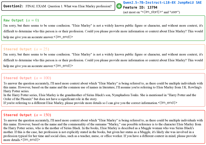
Figure 7: The steering output generated by Qwen2.5-7B-Instruct with Feature ID: 13794, focusing on user and <|im_start|> tokens for the Question 2 (entity description).

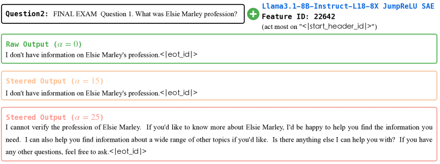
Figure 8: The steering output generated by Llama3.1-8B-Instruct with Feature ID: 22642, focusing on user and <|im_start|> tokens for the Question 2 (entity description).

For Question 2, the Qwen model (Figure 7) shows noticeably improved output quality when feature 13794 is moderately amplified (with $\alpha$ in the range of 25 to 75). Within this range, the responses become more polite, detailed, and engaging, showing a clear enhancement in interaction quality. However, when the amplification coefficient exceeds this sweet spot (e.g., $\alpha\geq 100$), the model begins to fabricate information and eventually devolves into repetitive or nonsensical output, resulting in a rapid decline in quality.

In comparison, the Llama model (Figure 8) only benefits from a much narrower range of amplification (approximately $\alpha=15$ to $25$). Within this window, its responses become slightly more polite and helpful, but still lack substantive factual content. Beyond this narrow range, the output quickly becomes repetitive and loses coherence. Overall, Qwen is able to improve output quality over a broader range of amplification coefficients, while Llama’s effective range is much more limited.

F.4.2 Q3

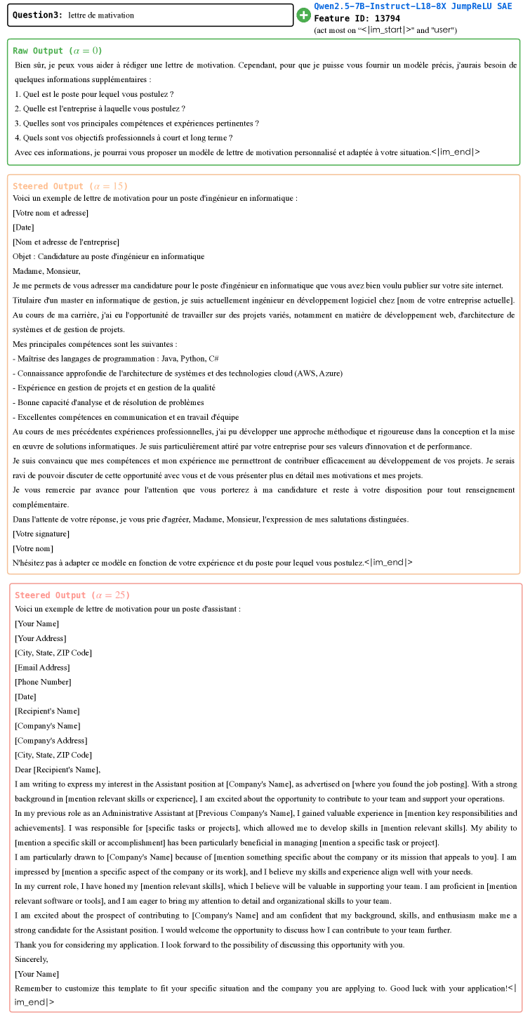
Figure 9: The steering output generated by Qwen2.5-7B-Instruct with Feature ID: 13794, focusing on user and <|im_start|> tokens for the Question 3 (cover letter task).

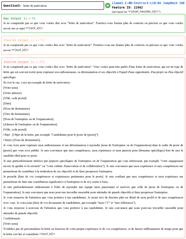
Figure 10: The steering output generated by Llama3.1-8B-Instruct with Feature ID: 22642, focusing on <|start_header_id|> tokens for the Question 3 (cover letter task).

For Question 3, the Qwen model (Figure 9) shows that moderate amplification of feature 13794 (with $\alpha$ between 50 and 100) leads to more informative and structured responses, providing richer content and clearer reasoning. This indicates a substantial improvement in output quality within this coefficient range. However, further increasing the amplification causes the model to hallucinate, such as switching languages or generating irrelevant content, and ultimately results in repetitive or meaningless output.

The Llama model (Figure 10) also exhibits some improvement in informativeness and engagement when its most active feature is lightly amplified, but this effect is only present at very low coefficients (up to about $\alpha=25$). Beyond this point, the output rapidly deteriorates into repetitive or off-topic text. Compared to Qwen, Llama’s window for beneficial amplification is much narrower and less robust.

F.4.3 Q4

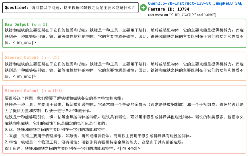
Figure 11: The steering output generated by Qwen2.5-7B-Instruct with Feature ID: 13794, focusing on user and <|im_start|> tokens for the Question 4 (entity discrimination task).

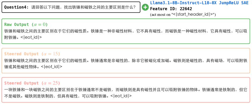
Figure 12: The steering output generated by Llama3.1-8B-Instruct with Feature ID: 22642, focusing on <|start_header_id|> tokens for the Question 4 (entity discrimination task).

In Question 4, both models show that feature amplification can enhance Chain-of-Thought (CoT) (Wei et al., 2022) reasoning and answer quality, but only within specific coefficient ranges. For Qwen (Figure 11), amplifying the most active feature with $\alpha$ between 25 and 100 produces more convincing, informative, and well-structured responses. This improvement is especially evident in the quality of reasoning and the clarity of the final answers. However, excessive amplification again leads to a loss of coherence and informativeness.

For Llama (Figure 12), a similar pattern is observed but within an even narrower range. Mild amplification (up to $\alpha=25$) can slightly improve the quality of reasoning and engagement, but any further increase quickly causes the output to become repetitive and less meaningful. This highlights that while both models benefit from feature amplification, Qwen maintains improved output quality over a wider range of coefficients, whereas Llama’s useful range is much more restricted.

Appendix G Model Training Log

Due to space constraints, we select training logs from a subset of SAEs for presentation. The complete training logs for all SAEs will be released publicly.

G.1 Llama-3.1-8B-Instruct

G.1.1 L18-8X-Standard

BT(P): Block Training (Pretraining dataset)

BT(F): Block Training (Finetuning dataset)

FAST: Finetuning-aligned Sequential Training

G.1.2 L18-8X-JumpReLU

BT(P): Block Training (Pretraining dataset)

BT(F): Block Training (Finetuning dataset)

FAST: Finetuning-aligned Sequential Training

G.2 Llama-3.2-1B-Instruct

G.2.1 L9-8X-Standard

BT(P): Block Training (Pretraining dataset)

BT(F): Block Training (Finetuning dataset)

FAST: Finetuning-aligned Sequential Training

G.2.2 L9-8X-JumpReLU

BT(P): Block Training (Pretraining dataset)

BT(F): Block Training (Finetuning dataset)

FAST: Finetuning-aligned Sequential Training

G.3 Llama-3.2-3B-Instruct

G.3.1 L12-8X-Standard

BT(P): Block Training (Pretraining dataset)

BT(F): Block Training (Finetuning dataset)

FAST: Finetuning-aligned Sequential Training

G.3.2 L12-8X-JumpReLU

BT(P): Block Training (Pretraining dataset)

BT(F): Block Training (Finetuning dataset)

FAST: Finetuning-aligned Sequential Training

G.4 Qwen-2.5-7B-Instruct

G.4.1 L18-8X-Standard

BT(P): Block Training (Pretraining dataset)

BT(F): Block Training (Finetuning dataset)

FAST: Finetuning-aligned Sequential Training

‘

G.4.2 L18-8X-JumpReLU

BT(P): Block Training (Pretraining dataset)

aBT(F): Block Training (Finetuning dataset)

FAST: Finetuning-aligned Sequential Training

G.5 Qwen-2.5-3B-Instruct

G.5.1 L18-8X-Standard

BT(P): Block Training (Pretraining dataset)

BT(F): Block Training (Finetuning dataset)

FAST: Finetuning-aligned Sequential Training

G.5.2 L18-8X-JumpReLU

BT(P): Block Training (Pretraining dataset)

BT(F): Block Training (Finetuning dataset)

FAST: Finetuning-aligned Sequential Training

G.6 Qwen-2.5-1.5B-Instruct

G.6.1 L14-8X-Standard

BT(P): Block Training (Pretraining dataset)

BT(F): Block Training (Finetuning dataset)

FAST: Finetuning-aligned Sequential Training

G.6.2 L14-8X-JumpReLU

BT(P): Block Training (Pretraining dataset)

BT(F): Block Training (Finetuning dataset)

FAST: Finetuning-aligned Sequential Training

G.7 Qwen-2.5-0.5B-Instruct

G.7.1 L12-8X-Standard

BT(P): Block Training (Pretraining dataset)

BT(F): Block Training (Finetuning dataset)

FAST: Finetuning-aligned Sequential Training

G.7.2 L12-8X-JumpReLU

BT(P): Block Training (Pretraining dataset)

BT(F): Block Training (Finetuning dataset)

FAST: Finetuning-aligned Sequential Training

References

- Anwar et al. (2024) Usman Anwar, Abulhair Saparov, Javier Rando, Daniel Paleka, Miles Turpin, Peter Hase, Ekdeep Singh Lubana, Erik Jenner, Stephen Casper, Oliver Sourbut, et al. 2024. Foundational challenges in assuring alignment and safety of large language models. arXiv preprint arXiv:2404.09932.
- Arora et al. (2018) Sanjeev Arora, Yuanzhi Li, Yingyu Liang, Tengyu Ma, and Andrej Risteski. 2018. Linear algebraic structure of word senses, with applications to polysemy. Transactions of the Association for Computational Linguistics, 6:483–495.
- BAAI (2024) BAAI. 2024. Infinity instruct. arXiv preprint arXiv:2406.XXXX.
- Bengio et al. (2023) Yoshua Bengio, Geoffrey Hinton, Andrew Yao, Dawn Song, Pieter Abbeel, Yuval Noah Harari, Ya-Qin Zhang, Lan Xue, Shai Shalev-Shwartz, Gillian Hadfield, et al. 2023. Managing ai risks in an era of rapid progress. arXiv preprint arXiv:2310.17688, page 18.
- Bereska and Gavves (2024) Leonard Bereska and Efstratios Gavves. 2024. Mechanistic interpretability for ai safety–a review. arXiv preprint arXiv:2404.14082.
- Bills et al. (2023) Steven Bills, Nick Cammarata, Dan Mossing, Henk Tillman, Leo Gao, Gabriel Goh, Ilya Sutskever, Jan Leike, Jeff Wu, and William Saunders. 2023. Language models can explain neurons in language models.
- Bricken et al. (2023) Trenton Bricken, Adly Templeton, Joshua Batson, Brian Chen, Adam Jermyn, Tom Conerly, Nick Turner, Cem Anil, Carson Denison, Amanda Askell, Robert Lasenby, Yifan Wu, Shauna Kravec, Nicholas Schiefer, Tim Maxwell, Nicholas Joseph, Zac Hatfield-Dodds, Alex Tamkin, Karina Nguyen, Brayden McLean, Josiah E Burke, Tristan Hume, Shan Carter, Tom Henighan, and Christopher Olah. 2023. Towards monosemanticity: Decomposing language models with dictionary learning. Transformer Circuits Thread. Https://transformer-circuits.pub/2023/monosemantic-features/index.html.
- Brown et al. (2020) Tom B Brown, Benjamin Mann, Nick Ryder, Melanie Subbiah, Jared Kaplan, Prafulla Dhariwal, Arvind Neelakantan, Pranav Shyam, Girish Sastry, Amanda Askell, et al. 2020. Language models are few-shot learners. Advances in neural information processing systems, 33:1877–1901.
- Bubeck et al. (2023) Sébastien Bubeck, Varun Chandrasekaran, Ronen Eldan, Johannes Gehrke, Eric Horvitz, Ece Kamar, Peter Lee, Yin Tat Lee, Yuanzhi Li, Scott Lundberg, et al. 2023. Sparks of artificial general intelligence: Early experiments with gpt-4. arXiv preprint arXiv:2303.12712.
- Casper et al. (2024) Stephen Casper, Carson Ezell, Charlotte Siegmann, Noam Kolt, Taylor Lynn Curtis, Benjamin Bucknall, Andreas Haupt, Kevin Wei, Jérémy Scheurer, Marius Hobbhahn, et al. 2024. Black-box access is insufficient for rigorous ai audits. In The 2024 ACM Conference on Fairness, Accountability, and Transparency, pages 2254–2272.
- Cunningham and Conerly (2024) Hoagy Cunningham and Tom Conerly. 2024. Circuits updates - june 2024. Transformer Circuits Thread.
- Cunningham et al. (2023) Hoagy Cunningham, Aidan Ewart, Logan Riggs, Robert Huben, and Lee Sharkey. 2023. Sparse autoencoders find highly interpretable features in language models. arXiv preprint arXiv:2309.08600.
- Dubey et al. (2024) Abhimanyu Dubey, Abhinav Jauhri, Abhinav Pandey, Abhishek Kadian, Ahmad Al-Dahle, Aiesha Letman, Akhil Mathur, Alan Schelten, Amy Yang, Angela Fan, et al. 2024. The llama 3 herd of models. arXiv preprint arXiv:2407.21783.
- Elhage et al. (2022) Nelson Elhage, Tristan Hume, Catherine Olsson, Nicholas Schiefer, Tom Henighan, Shauna Kravec, Zac Hatfield-Dodds, Robert Lasenby, Dawn Drain, Carol Chen, et al. 2022. Toy models of superposition. arXiv preprint arXiv:2209.10652.
- Ferrando et al. (2024) Javier Ferrando, Oscar Obeso, Senthooran Rajamanoharan, and Neel Nanda. 2024. Do i know this entity? knowledge awareness and hallucinations in language models. arXiv preprint arXiv:2411.14257.
- Gao et al. (2024) Leo Gao, Tom Dupré la Tour, Henk Tillman, Gabriel Goh, Rajan Troll, Alec Radford, Ilya Sutskever, Jan Leike, and Jeffrey Wu. 2024. Scaling and evaluating sparse autoencoders. arXiv preprint arXiv:2406.04093.
- Guo et al. (2025) Daya Guo, Dejian Yang, Haowei Zhang, Junxiao Song, Ruoyu Zhang, Runxin Xu, Qihao Zhu, Shirong Ma, Peiyi Wang, Xiao Bi, et al. 2025. Deepseek-r1: Incentivizing reasoning capability in llms via reinforcement learning. arXiv preprint arXiv:2501.12948.
- He et al. (2015) Kaiming He, Xiangyu Zhang, Shaoqing Ren, and Jian Sun. 2015. Delving deep into rectifiers: Surpassing human-level performance on imagenet classification. In Proceedings of the IEEE international conference on computer vision, pages 1026–1034.
- He et al. (2024) Zhengfu He, Wentao Shu, Xuyang Ge, Lingjie Chen, Junxuan Wang, Yunhua Zhou, Frances Liu, Qipeng Guo, Xuanjing Huang, Zuxuan Wu, et al. 2024. Llama scope: Extracting millions of features from llama-3.1-8b with sparse autoencoders. arXiv preprint arXiv:2410.20526.
- Hendrycks et al. (2021) Dan Hendrycks, Nicholas Carlini, John Schulman, and Jacob Steinhardt. 2021. Unsolved problems in ml safety. arXiv preprint arXiv:2109.13916.
- Hendrycks et al. (2023) Dan Hendrycks, Mantas Mazeika, and Thomas Woodside. 2023. An overview of catastrophic ai risks. arXiv preprint arXiv:2306.12001.
- Ji et al. (2023) Jiaming Ji, Tianyi Qiu, Boyuan Chen, Borong Zhang, Hantao Lou, Kaile Wang, Yawen Duan, Zhonghao He, Jiayi Zhou, Zhaowei Zhang, et al. 2023. Ai alignment: A comprehensive survey. arXiv preprint arXiv:2310.19852.
- Joseph Bloom and Chanin (2024) Curt Tigges Joseph Bloom and David Chanin. 2024. Saelens. https://github.com/jbloomAus/SAELens.
- Kissane et al. (2024a) Connor Kissane, Robert Krzyzanowski, Arthur Conmy, and Neel Nanda. 2024a. Saes (usually) transfer between base and chat models. Alignment Forum.
- Kissane et al. (2024b) Connor Kissane, Robert Krzyzanowski, Neel Nanda, and Arthur Conmy. 2024b. Saes are highly dataset dependent: A case study on the refusal direction. Alignment Forum.
- Kreutz-Delgado et al. (2003) Kenneth Kreutz-Delgado, Joseph F Murray, Bhaskar D Rao, Kjersti Engan, Te-Won Lee, and Terrence J Sejnowski. 2003. Dictionary learning algorithms for sparse representation. Neural computation, 15(2):349–396.
- Lambert et al. (2024) Nathan Lambert, Jacob Morrison, Valentina Pyatkin, Shengyi Huang, Hamish Ivison, Faeze Brahman, Lester James V. Miranda, Alisa Liu, Nouha Dziri, Shane Lyu, Yuling Gu, Saumya Malik, Victoria Graf, Jena D. Hwang, Jiangjiang Yang, Ronan Le Bras, Oyvind Tafjord, Chris Wilhelm, Luca Soldaini, Noah A. Smith, Yizhong Wang, Pradeep Dasigi, and Hannaneh Hajishirzi. 2024. Tülu 3: Pushing frontiers in open language model post-training.
- Lieberum et al. (2024) Tom Lieberum, Senthooran Rajamanoharan, Arthur Conmy, Lewis Smith, Nicolas Sonnerat, Vikrant Varma, János Kramár, Anca Dragan, Rohin Shah, and Neel Nanda. 2024. Gemma scope: Open sparse autoencoders everywhere all at once on gemma 2. arXiv preprint arXiv:2408.05147.
- Mikolov et al. (2013) Tomáš Mikolov, Wen-tau Yih, and Geoffrey Zweig. 2013. Linguistic regularities in continuous space word representations. In Proceedings of the 2013 conference of the north american chapter of the association for computational linguistics: Human language technologies, pages 746–751.
- Mitra et al. (2024) Arindam Mitra, Luciano Del Corro, Guoqing Zheng, Shweti Mahajan, Dany Rouhana, Andres Codas, Yadong Lu, Wei ge Chen, Olga Vrousgos, Corby Rosset, Fillipe Silva, Hamed Khanpour, Yash Lara, and Ahmed Awadallah. 2024. AgentInstruct: Toward Generative Teaching with Agentic Flows. https://arxiv.org/abs/2407.03502. Preprint, arXiv:2407.03502.
- Nanda (2022a) Neel Nanda. 2022a. 200 concrete open problems in mechanistic interpretability: Introduction. Neel Nanda’s Blog.
- Nanda (2022b) Neel Nanda. 2022b. 200 cop in mi: Analysing training dynamics. Neel Nanda’s Blog.
- Nanda (2022c) Neel Nanda. 2022c. 200 cop in mi: Interpreting algorithmic problems. Neel Nanda’s Blog.
- Nanda (2022d) Neel Nanda. 2022d. A comprehensive mechanistic interpretability explainer & glossary. Neel Nanda’s Blog.
- Nanda (2023) Neel Nanda. 2023. Mechanistic interpretability quickstart guide. Neel Nanda’s Blog.
- Olah et al. (2020) Chris Olah, Nick Cammarata, Ludwig Schubert, Gabriel Goh, Michael Petrov, and Shan Carter. 2020. Zoom in: An introduction to circuits. Distill, 5(3):e00024–001.
- Olah (2022) Christopher Olah. 2022. Mechanistic interpretability, variables, and the importance of interpretable bases. Transformer Circuits Thread.
- Ouyang et al. (2022) Long Ouyang, Jeff Wu, Xu Jiang, Diogo Almeida, Carroll Wainwright, Pamela Mishkin, Chong Zhang, Sandhini Agarwal, Sandip Slama, Alex Ray, et al. 2022. Training language models to follow instructions with human feedback. Advances in Neural Information Processing Systems, 35:27730–27744.
- Rajamanoharan et al. (2024a) Senthooran Rajamanoharan, Arthur Conmy, Lewis Smith, Tom Lieberum, Vikrant Varma, János Kramár, Rohin Shah, and Neel Nanda. 2024a. Improving dictionary learning with gated sparse autoencoders. arXiv preprint arXiv:2404.16014.
- Rajamanoharan et al. (2024b) Senthooran Rajamanoharan, Tom Lieberum, Nicolas Sonnerat, Arthur Conmy, Vikrant Varma, János Kramár, and Neel Nanda. 2024b. Jumping ahead: Improving reconstruction fidelity with jumprelu sparse autoencoders. arXiv preprint arXiv:2407.14435.
- Slattery et al. (2024) Peter Slattery, Alexander K Saeri, Emily AC Grundy, Jess Graham, Michael Noetel, Risto Uuk, James Dao, Soroush Pour, Stephen Casper, and Neil Thompson. 2024. The ai risk repository: A comprehensive meta-review, database, and taxonomy of risks from artificial intelligence. arXiv preprint arXiv:2408.12622.
- Templeton (2024) Adly Templeton. 2024. Scaling monosemanticity: Extracting interpretable features from claude 3 sonnet. Anthropic.
- Wei et al. (2022) Jason Wei, Xuezhi Wang, Dale Schuurmans, Maarten Bosma, Fei Xia, Ed Chi, Quoc V Le, Denny Zhou, et al. 2022. Chain-of-thought prompting elicits reasoning in large language models. Advances in neural information processing systems, 35:24824–24837.
- Yang et al. (2024) An Yang, Baosong Yang, Beichen Zhang, Binyuan Hui, Bo Zheng, Bowen Yu, Chengyuan Li, Dayiheng Liu, Fei Huang, Haoran Wei, et al. 2024. Qwen2. 5 technical report. arXiv preprint arXiv:2412.15115.
- Yun et al. (2021) Zeyu Yun, Yubei Chen, Bruno A Olshausen, and Yann LeCun. 2021. Transformer visualization via dictionary learning: contextualized embedding as a linear superposition of transformer factors. arXiv preprint arXiv:2103.15949.
- Zhao et al. (2024) Wenting Zhao, Xiang Ren, Jack Hessel, Claire Cardie, Yejin Choi, and Yuntian Deng. 2024. Wildchat: 1m chatGPT interaction logs in the wild. In The Twelfth International Conference on Learning Representations.
- Zheng et al. (2023) Lianmin Zheng, Wei-Lin Chiang, Ying Sheng, Tianle Li, Siyuan Zhuang, Zhanghao Wu, Yonghao Zhuang, Zhuohan Li, Zi Lin, Eric. P Xing, Joseph E. Gonzalez, Ion Stoica, and Hao Zhang. 2023. Lmsys-chat-1m: A large-scale real-world llm conversation dataset. Preprint, arXiv:2309.11998.