Real-Time High-Accuracy Digital Wireless Time, Frequency, and Phase Calibration for Coherent Distributed Antenna Arrays

Abstract

This work presents a fully-digital high-accuracy real-time calibration procedure for frequency and time alignment of open-loop wirelessly coordinated cda modems, enabling rf phase coherence of spatially separated cots sdr without cables or external references such as gnss. Building on previous work using high-accuracy spectrally-sparse toa waveforms and a multi-step toa refinement process, a high-accuracy twtt-based time–frequency coordination approach is demonstrated. Due to the two-way nature of the high-accuracy twtt approach, the time and frequency estimates are Doppler and multi-path tolerant, so long as the channel is reciprocal over the synchronization epoch. This technique is experimentally verified using cots sdr in a lab environment in static and dynamic scenarios and with significant multipath scatterers. Time, frequency, and phase stability were evaluated by beamforming over coaxial cables to an oscilloscope which achieved time and phase precisions of $\sim$$60\text{\,}\mathrm{ps}$–$70\text{\,}\mathrm{ps}$, with median coherent gains above 99 % using optimized coordination parameters, and a beamforming frequency rmse of 3.73 ppb in a dynamic scenario. Finally, experiments were conducted to compare the performance of this technique with previous works using an analog cwtt frequency reference technique in both static and dynamic settings.

Nomenclature

General Notation

• $x_{0}$

  Nominal value of some quantity $x$ at $t=0$.

• $\hat{x}$

  Estimated value of some parameter $x$.

• $\tilde{x}$

  Compensation value to be applied to $x$.

• $\bar{x}$

  Apparent value of $x$ due to unsynchronized clocks.

• $x^{(n)}$

  Value specific to the $n$th node.

• $\delta g(x)$

  Linearly separable deviation of $g(x)$ from its ideal value. Defined as $\delta g(x)\equiv g(x)-g_{0}$.

• $\Delta g(x)$

  Dimensionless ratio representing the fractional error relative to the nominal value. Defined as $\Delta g(x)\equiv\delta g(x)/g_{0}$.

• $g^{(n,m)}(x)$

  Difference between the value $g(x)$ at nodes $n$ and $m$. Defined by $g^{(n,m)}(x)\equiv g^{(m)}(x)-g^{(n)}(x)\equiv-[g^{(n)}(x)-g^{(m)}(x)]$.

Quantities

• $\phi(t)$

  Instantaneous phase in radians.

• $\delta\phi(t)$

  Instantaneous phase deviation in radians.

• $T(t)$

  Total accumulated time of a timebase in seconds. Defined by $T(t)\equiv\phi(t)/(2\pi f_{0})\equiv t+\delta\phi(t)/(2\pi f_{0})$.

• $\delta T(t)$

  Total accumulated time error of a timebase in seconds. Defined by $\delta T(t)\equiv T(t)-t\equiv\delta{\phi}(t)/(2\pi f_{0})$.

• $f(t)$

  Instantaneous Fourier frequency in Hertz. Defined by $f(t)\equiv\frac{\mathrm{d}}{\mathrm{d}t}\phi(t)/(2\pi)$.

• $\delta f(t)$

  Instantaneous Fourier frequency error in Hertz. Defined by $\delta{f}(t)\equiv f(t)-f_{0}$.

• $\Psi(t)$

  Modulation phase of some information.

• $R^{(n,m)}(t)$

  Radial distance between nodes $n$ and $m$.

• $v_{r}^{(n,m)}(t)$

  Radial velocity between nodes $n$ and $m$. Defined by $v_{r}^{(m,n)}\equiv\mathrm{d}R^{(m,n)}(t)/\mathrm{d}t$.

• $f_{d}^{(n,m)}(t)$

  Doppler shift observed between nodes $n$ and $m$.

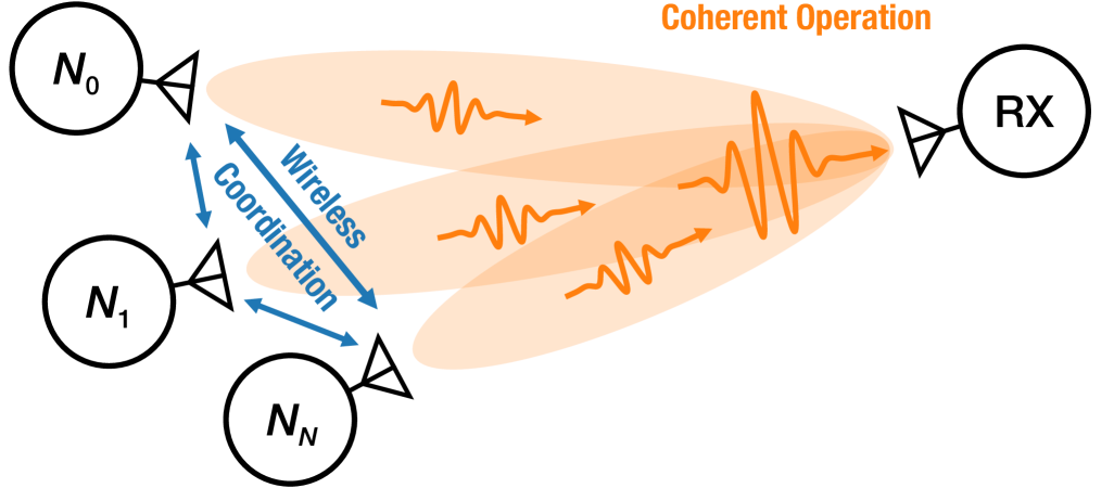
Figure 1: Distributed array concept for an $N$-element array. Each element in the array coordinates wirelessly to align its electrical state (time, frequency, and phase) to perform a coherent operation, such as beamforming. In this example, the receiver, labelled RX, can be a conventional active receiver modem, or a passive feature of interest in a radar-type operation.

I Introduction

Wirelessly coordinated cda, shown schematically in Fig. 1, have been growing in interest in a range of applications spanning from radar imaging and remote sensing [1, 2, 3, 4, 5, 6, 7, 8, 9, 10], automotive radar [11, 12, 13, 14], and wireless power transfer [15, 16, 17], to secure wireless communications [18], next generation terrestrial wireless communications [19, 20, 21, 22], and deep space communication networks [23], [24, TX05.2.6]. The motivation for this growing interest in wireless cda, instead of a traditional monolithic array, is driven by several factors [25]:

1. Scalability: Wirelessly coordinated cda can be easily scaled and adapted to changing conditions due to the mobile nature of each element. New elements can be added or removed over time or when elements fail, potentially reducing deployment and operational costs. Additionally, since each element in the array contains its own power source, the overall array transmit gain increases with $N^{2}$ as the array size increases, while mitigating the challenges of cooling similarly large monolithic arrays.

2. Adaptability: Because the elements are mobile, the array geometry can be changed to operate efficiently over wide bandwidths, or to optimize the array pattern for a specific operating mode (e.g., radar or communications) by changing the element positions.

3. Reliability: Because the functions of a cda can be spread across multiple nodes, the array may be designed such that there is no single point of failure should a node become inoperable. Furthermore, due to the larger spatial diversity compared to a densely filled monolithic array, the array can be more resilient to interference and multipath fading and can improve sensing performance of specular objects in a radar operating mode.

To achieve these benefits, the electrical states—time, phase, and frequency—of each system must be aligned to ensure all elements operate coherently. This can be accomplished by either providing feedback from a cooperative destination, forming a closed-loop system [26, 27, 28, 29, 30, 31, 32, 33, 34], or by communicating the electrical states directly between nodes in the array, forming an open-loop system [35, 36, 37, 38, 39, 40, 1, 41, 42, 43, 9, 6, 44, 19, 45, 46, 47]. While closed-loop topologies are often simpler to implement, they suffer from the fact that individual elements must still be able to receive feedback from the destination, requiring sufficient single-element snr; furthermore, closed-loop systems inherently require feedback from the receiver, and thus, cannot support communication with conventional modems or radar remote sensing operations. Open-loop cda can support any operating mode that a conventional antenna array can support but are more challenging to implement as the exact location, time, frequency, and phase offsets of all nodes must be coordinated directly between elements to a fraction of the carrier wavelength to support fully-coherent operation [35]. To accomplish this, a standard timebase for the array which describes the current time and the rate at which it passes, i.e., frequency, must be agreed upon. In general, there are two methods of selecting a timebase in an array: centralized in which single node is elected to act as the primary timebase that disseminates its time and frequency to all other nodes in the array [36, 37, 41, 39, 42, 43, 9, 19], or decentralized in which all elements in the array collectively converge to a mean time and frequency value [38, 40, 6, 44]; however, in some cases, a combination of these approaches is employed [1, 45]. Typically, in centralized arrays, a star topology is used, where all secondary nodes receive information directly from the primary node; however, repeaters can be employed but will degrade the coordination accuracy of the array with each re-transmission. In a decentralized array, nodes only monitor the electrical states of their neighboring nodes and adjust their values to the average of its neighbors’ and its own values. Because of this, the array topology is less strict, requiring only that all nodes have at least one edge connected to another node in the array. Centralized topologies are often simpler to implement and have the advantage of being able to synchronize the entire array in a single epoch (an atomic synchronization operation), while fully decentralized arrays are more involved and require multiple epochs to reach convergence, but are robust to any node entering and exiting the array at random. In this work, we discuss a centralized technique for simplicity, focusing on the electrical state estimation aspect of the coordination challenge; however, because this approach is fully digital (i.e., does not rely on any centralized analog reference hardware), a decentralized consensus-based technique, such as average consensus for undirected networks [48, 1, 40, 49, 50, 6, 45], or push-sum techniques for directed networks [51], can easily be employed.

Once a timebase has been determined, the challenge of accurately comparing time, frequency, and phase offsets between elements within the array remains. In a spatially distributed network of sdr, each radio will have its own free-running reference oscillator whose frequency of oscillation will fluctuate on many time scales due to varying intrinsic and extrinsic factors such as aging, temperature, pressure, and acceleration, to name a few. Because the radios are distributed spatially—potentially on moving platforms—each radio will experience different extrinsic influences causing the oscillators to vary in an uncorrelated manner. Commonly, the task of phase estimation and correction is decomposed into three independent tasks, starting with either synchronization (time alignment) or syntonization (frequency alignment), which must be performed continuously, followed by static phase corrections to correct for the rfe and antenna phase pattern, which can be performed prior to system operation. The task of time estimation can be accomplished using either one-way, or two-way techniques. One-way techniques have been implemented successfully in ntp and gnss time and frequency distribution; however, these techniques require the csi and relative location and velocity of each node to be well-characterized to achieve high levels of accuracy, which is not always practical in a cda. In situations where csi is not available, twtt-based techniques can be used in which the impact of the channel on internode time and phase measurements is implicitly cancelled by the two-way process, assuming it is quasi-static over the synchronization epoch [52, 53, 54]; a common implementation of this is IEEE-1588 ptp, which can achieve synchronization to the microsecond-level in computer networks [55] and has recently been extended to include a high-accuracy profile based on White Rabbit to achieve sub-nanosecond levels of synchronization [56]. Several high-accuracy twtt-based techniques have been experimentally demonstrated in the context of rf wirelessly coordinated cda, typically involving a multi-stage refinement technique to achieve toa estimate accuracies significantly below the sampling period of the platform [57, 1]. This technique is expanded upon in [58] and [42] taking advantage of the cooperative nature of the cda system by leveraging spectrally-sparse two-tone toa waveforms which minimize the variance on the toa estimation while mitigating range-Doppler coupling when compared with the lfm waveforms commonly used in cda coordination. Frequency syntonization is commonly performed independently of time synchronization either directly via a continuous frequency reference broadcast and analog reception circuit, which is used to discipline the lo of secondary nodes [36, 59, 41, 42, 60], or indirectly via digital spectral estimation of pulsed tones which are typically either estimated in the Fourier frequency domain digitally using peak estimation [32, 9, 6, 44] or via carrier phase tracking over sequential pulses with sufficient periodicity to mitigate ambiguity [37, 34, 19]. Similarly to time-transfer, these techniques can also be separated into one-way and two-way methods, with the latter being robust to Doppler shift, so long as the frequency shift is constant over a syntonization epoch [6].

In this work, we build on our previous research on high-accuracy wireless time coordination [42] while implementing an indirect digital frequency estimation technique by tracking the time drift of the reference oscillators. This technique takes advantage of the fact that the rf lo on a typical sdr platform will, on average, have the same fractional frequency error as the system clock which it is derived from. Because of this, if the frequency error of the system clock can be estimated with a time jitter significantly lower than the lo period, the frequency error of the carrier can be indirectly estimated and compensated for. This technique has several advantages over direct carrier spectral estimation and sequential carrier phase estimation techniques:

1. Unambiguity: The twtt technique directly estimates the system clock’s time instead of the carrier phase; thus, there is no ambiguity resolution required unlike sequential carrier phase estimate-based techniques.

2. Low Duty Cycle: The variance of the twtt-based frequency estimation is minimized by having short twtt exchanges separated by a large amount of time, whereas the variance of spectral estimation techniques is minimized by integrating long duration frequency pulses. Because of this, the twtt-based frequency estimation technique can provide lower variance estimates while maintaining low coordination overhead for the array.

3. Doppler and Multipath Tolerance: The twtt-based technique estimates the time independent of time-varying channel state from multipath and Doppler shift, due to its two-way nature, so long as the channel is quasi-static over the synchronization epoch (i.e., the epoch is short relative to the evolution of the channel). While two-way spectral frequency estimates also separate the platform electrical states from the channel state, the requirement for increasing pulse duration to improve frequency estimation conflicts with the requirement to minimize the synchronization epoch duration to improve performance in time-varying channels.

In [42] it was shown that the high-accuracy twtt technique could synchronize the system on the order of picoseconds, which should be sufficient to support beamforming directly at microwave frequencies based on prior analyses [35]. In this paper, we demonstrate this experimentally by sending a “beamforming” pulse via cables to independent channels on an oscilloscope to measure the individual electrical state coordination performance of each system during operation while it is performing fully wireless coordination. Over several experiments we demonstrate the practical array performance with incoherent clock sources and with coherent clock sources with a known fixed relative frequency offset between platforms to measure the lower bound on time and frequency estimation performance, and we compare it to the hybrid digital twtt and analog wireless frequency syntonization technique described in [42]. In several experiments a linear guide is also used to induce Doppler shift with multiple large scatterers placed nearby to induce multipath. In these experiments we demonstrate time and phase coordination standard deviations of $\sim$$60\text{\,}\mathrm{ps}$–$70\text{\,}\mathrm{ps}$ at 27 dB snr and a median coherent gain of 99 % in static and dynamic scenarios in the system with incoherent clocks, and an internode beamforming frequency rmse of below 5 ppb in static and dynamic scenarios in a two-node array.

The remainder of the paper will proceed as follows. Section II-A will discuss the intranode signal model which describes the electrical states (i.e., time, frequency, and phase) and the separate error sources which impact them, and its impact on transmitted and received waveforms; Section II-B describes the internode signal model describing the relative error in electrical states between nodes. In Section III the high-accuracy two-way time and frequency estimation technique is described and their lower bounds on variance are presented. Section IV describes the fully-digital phase compensation technique employed to correct for the estimated time and frequency errors. Finally, Section V will detail the experiments used to verify the performance of the proposed techniques.

II Signal Model

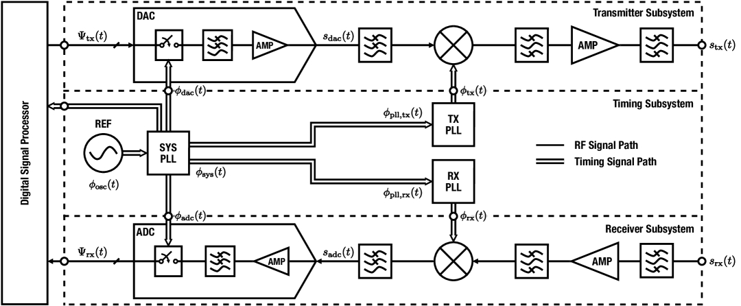
Figure 2: Simplified single channel full-duplex sdr schematic used for system modeling. In general, all phase quantities are slowly time-varying with respect to changing extrinsic and intrinsic conditions such as device temperature, drive levels, and acceleration, among others.

In this work we consider an array of $N$ sdr consisting of a typical direct conversion front end as shown in Fig. 2. The goal is for each of the sdr to operate in phase coherence as if they shared the same frequency reference in order to achieve an active coherent array transmit gain of $N^{2}$; however, errors, primarily induced by the timing subsystem, will induce carrier frequency offset, sampling frequency offset (time scaling), and carrier and sampling phase wander. In a distributed array, all these effects must be estimated and compensated for to ensure that the waveforms transmitted and received at each element are in phase at any given time, supporting beamforming operation.

II-A Intranode Signal Model

From a signal perspective, the system may be broken into the transmitter, receiver, and timing subsystems, as shown in Fig. 2. Following the signal from the perspective of the transmitter and receiver subsystems, each have four ports: the baseband signal at the data converters $\Psi_{\mathrm{tx}}(t),\Psi_{\mathrm{rx}}(t)$; the sample clocks $\phi_{\mathrm{dac}}(t),\phi_{\mathrm{adc}}(t)$; the lo $\phi_{\mathrm{tx}}(t),\phi_{\mathrm{rx}}(t)$, which are often independently tunable; and the rf ports $s_{\mathrm{tx}}(t),s_{\mathrm{rx}}(t)$. It should also be noted that a direct rf sampling sdr would behave in a similar manner, with the mixers being replaced by the data converters, using the lo to drive the sample clocks, eliminating the phase uncertainty between the data converter clocks and lo. To properly model the effect the system has on the transmitted and received waveforms, the impact of each subsystem must be modeled.

II-A1 Timing Subsystem

The goal of the timing subsystem is to create a time and frequency reference which is true to an agreed upon frequency standard over the course of operation; however, practical challenges such as size, weight, power consumption and cost limit the options available for sdr. Often, all of these parameters are minimized leading to the use of some form of crystal oscillators as the primary frequency reference in an sdr, which typically have lower long-term stability and are more susceptible to environmental conditions than atomic frequency standards. Environmental impacts such as temperature, pressure, humidity, and acceleration [61, 62, 63, 64, 65] can all impact the frequency of oscillation, as well as initial manufacturing tolerance, crystal contamination creating loading, and internal crystalline structure changes, which can all contribute to aging frequency drift [66, 67, 68, 69]. Aging is typically a slow process with fractional frequency drifts on the order of $1\times 10^{-9}/$day for new crystals to $1\times 10^{-12}/$day after several months [68, 69] and can be easily compensated by periodic recalibration over days. Environmental impacts on frequency are more challenging to mitigate. Typically, crystal oscillators are hermetically sealed to isolate them from contaminants, humidity, and pressure changes, and either temperature compensated (TCXO) or oven controlled (OCXO) by a heating element to keep the crystal at a constant temperature. While these minimize the impacts of environmental disturbances, they cannot be fully eliminated. Furthermore, on a moving platform, the impact of vibration and acceleration is very challenging to eliminate entirely, though various techniques have been implemented [65, 70]. Because the sources of environmental disturbances can be viewed as a random process, the impact of these sources on the oscillator phase can also be viewed as a random process inducing phase noise. Temperature and pressure changes typically induce phase noise very close to the carrier, while accelerations and vibration may produce spurs or phase noise at frequencies further from the carrier. The resulting signal from the reference oscillator can be modeled as

$$\begin{split}\phi_{\mathrm{osc}}(t)&=2\pi f_{\mathrm{0,osc}}\left[1+\Delta f_{\mathrm{osc}}(t)\right]t+\nu_{\phi,\mathrm{osc}}(t)+\phi_{0,\mathrm{osc}}.\end{split}$$ (1)

Figure 3: Simplified pll synthesizer model. Noise is added at each stage in the loop and the frequency and noise are magnified by the feedback ratio $\kappa$.

Figure 4: Phase noise profile of a pll synthesizer, where $\kappa$ is the feedback divider ratio. The loop filter cutoff frequency is indicated by $f_{c}$ and $S_{\phi,0}$ is the noise floor of the pll due to intrinsically generated noises.

where $\Delta f_{\mathrm{osc}}(t)=\delta f_{\mathrm{0,osc}}(t)/f_{\mathrm{0,osc}}$ is a fractional frequency error due to initial manufacturing defects and aging; $\delta f_{\mathrm{0,osc}}(t)$ is the absolute frequency error and the $f_{\mathrm{0,osc}}$ is the nominal frequency of the reference oscillator; and $\phi_{\mathrm{0,osc}}$ is the initial phase of the oscillator. The quantity $\nu_{\phi,\mathrm{osc}}(t)$ is the stationary zero mean random phase noise process which can be described by a gaussian power spectral density very near the carrier [71, 72] and a power law at further out frequencies [61, 73], [74, §7.3], [75, §2.2]. This signal is then passed to the system pll synthesizer (SYS PLL)—shown schematically in Fig. 3—to generate a higher frequency reference for the dsp, data converters, and the lo pll synthesizers. In general, pll act as a low-pass filter for phase noise from the reference source and the intrinsically generated phase noises due to resistive and active components, and a high-pass filter for vco noise. An approximation of the phase noise profile at the output of a pll synthesizer is shown in Fig. 4. The phase at the output of the SYS PLL can be modeled as the sum of the ideal output frequency and a time-varying phase error

$$\begin{split}\phi_{\mathrm{sys}}(t)&=2\pi f_{\mathrm{0,sys}}t+\delta\phi_{\mathrm{sys}}(t)\end{split}$$ (2)

where

$$\delta\phi_{\mathrm{sys}}(t)=2\pi f_{\mathrm{0,sys}}\Delta f_{\mathrm{osc}}t+\nu_{\phi,\mathrm{sys}}(t)+\phi_{\mathrm{0,sys}}$$ (3)

and $f_{\mathrm{0,sys}}=\kappa_{\mathrm{sys}}f_{\mathrm{0,osc}}$ where $\kappa_{\mathrm{sys}}$ is the feedback scaling factor for frequency multiplication, $\nu_{\phi,\mathrm{sys}}(t)=\kappa_{\mathrm{sys}}\langle\nu_{\phi,\mathrm{sys,in}}(t)+\nu_{\phi,\mathrm{osc}}(t)\rangle_{\mathrm{lpf}}+\langle\nu_{\phi,\mathrm{vco}}(t)\rangle_{\mathrm{hpf}}$ where $\nu_{\phi,\mathrm{sys,in}}(t)$ is the intrinsically generated phase noise, $\nu_{\phi,\mathrm{vco}}(t)$ is the phase noise generated by the vco, and $\langle\cdot\rangle_{\mathrm{lpf}}$ and $\langle\cdot\rangle_{\mathrm{hpf}}$ are ideal low-pass and high-pass filters, respectively. The term $\phi_{\mathrm{0,sys}}$ is the static phase shift due to signal propagation delays and the initial random phase offset of the reference oscillator.

The data converters and rf pll all behave in a similar manner; in addition, some dac will include integrated pll synthesizers and perform interpolation on the device to minimize analog filtering requirements. But in general, these can be viewed as adding a static phase delay and additional frequency scaling, while retaining the same fractional frequency stability as the reference oscillator. Here we will define the TX pll lo signal at the input of the mixer; the RX pll lo and data converter clocks $\phi_{\mathrm{dac}}(t)$ and $\phi_{\mathrm{adc}}(t)$ can be described similarly but are omitted for brevity. Starting with (2) a second frequency scaling factor will be added $\kappa_{\mathrm{tx}}$; for the transmitter lo letting $f_{\mathrm{0,tx}}=\kappa_{\mathrm{sys}}\kappa_{\mathrm{tx}}f_{\mathrm{0,osc}}$ yields

$$\begin{split}\phi_{\mathrm{tx}}(t)&=2\pi f_{\mathrm{0,tx}}t+\delta\phi_{\mathrm{tx}}(t)\end{split}$$ (4)

where

$$\delta\phi_{\mathrm{tx}}(t)=2\pi f_{\mathrm{0,tx}}\Delta f_{\mathrm{osc}}t+\nu_{\mathrm{\phi,\mathrm{tx}}}(t)+\phi_{\mathrm{0,tx}}$$ (5)

and $\nu_{\mathrm{\phi,\mathrm{tx}}}(t)$ is the summation of all phase noises at the lo induced by the pll as well as the phase errors from environmental perturbations and oscillator aging, and $\phi_{\mathrm{0,tx}}$ is the static phase offset due to propagation delay of the signal between the SYS PLL and TX PLL. The receiving lo can be modeled in the same way. It’s important to note that while $\nu_{\mathrm{\phi,sys}}(t)$ and $\nu_{\mathrm{\phi,tx}}(t)$ are represented as unique phase noise terms, these will be partially correlated noises deviating primarily at high offset frequencies from the carrier due to vco noises.

For further analysis it is useful to consider the continuous representation of time in seconds derived from a frequency reference, which is obtained from total accumulated phase divided by its nominal angular frequency

$$T(t)=\frac{\phi(t)}{2\pi f_{0}}=t+\frac{\delta\phi(t)}{2\pi f_{0}}=t+\delta T(t).$$ (6)

From (6), it’s clear that our notion of time—the accumulated phase at any given point in space—is relative to a given reference plane as well as the true angular rate of the phase $\mathrm{d}\,\phi(t)/\mathrm{d}t$; because the true value of frequency is not known, if the current angular rate of the phase is slower or faster than the expected frequency, the time will appear to run slower or faster relative to the global true time. In the case of system timing distribution, letting $\phi(t)\equiv\phi_{\mathrm{sys}}(t)$, (6) would become $T_{\mathrm{sys}}(t)$ representing the time at the output of the system frequency reference (SYS PLL); all components and transmission lines thereafter impart a phase shift on the timing signal path relative to this source.

II-A2 Transmitter Subsystem

From the transmitter perspective, a baseband signal $\Psi_{\mathrm{tx}}(t)$ is generated in the dsp, loaded into the dac sample registers and shifted out at the rate of the sampling clock given by $f_{\mathrm{s,dac}}(t)=\mathrm{d}\,\phi_{\mathrm{sys}}(t-\tau_{\mathrm{dac}})/2\pi\,\mathrm{d}t$ where $\tau_{\mathrm{dac}}$ is the propagation delay for the signal to travel from the SYS PLL output to the clocking circuit on the dac; because the clock signal is periodic, a time delay is indistinguishable from a phase shift, thus $\tau_{\mathrm{dac}}$ can be grouped with the static phase term $\phi_{\mathrm{0,dac}}$. The waveform at the output of the sampler can be modeled as a pulse train of sampling impulses, whose bandwidths are determined by the analog bandwidth of the sampler and output filters $\beta_{\mathrm{dac}}$, with a sampling period $T_{\mathrm{s,dac}}=1/f_{\mathrm{s,dac}}$; for simplicity, we will assume that $f_{\mathrm{s,dac}}=f_{\mathrm{0,sys}}=1/T_{\mathrm{0,sys}}$, yielding a reconstructed signal modeled by

$$\begin{split}s_{\mathrm{dac}}(t)&=\begin{multlined}\sum_{k}\Psi_{\mathrm{tx}}(kT_{\mathrm{0,sys}})\operatorname{sinc}\left\{\beta_{\mathrm{dac}}[t-T_{\mathrm{dac}}(kT_{\mathrm{0,sys}})]\right\}\end{multlined}\sum_{k}\Psi_{\mathrm{tx}}(kT_{\mathrm{0,sys}})\operatorname{sinc}\left\{\beta_{\mathrm{dac}}[t-T_{\mathrm{dac}}(kT_{\mathrm{0,sys}})]\right\}\\ &=\!\begin{multlined}\sum_{k}\Psi_{\mathrm{tx}}(kT_{\mathrm{0,sys}})\\ \times\operatorname{sinc}\bigg{\{}\beta_{\mathrm{dac}}\bigg{[}t-kT_{\mathrm{0,sys}}-\delta T_{\mathrm{dac}}(kT_{\mathrm{0,sys}})\bigg{]}\bigg{\}}\end{multlined}\sum_{k}\Psi_{\mathrm{tx}}(kT_{\mathrm{0,sys}})\\ \times\operatorname{sinc}\bigg{\{}\beta_{\mathrm{dac}}\bigg{[}t-kT_{\mathrm{0,sys}}-\delta T_{\mathrm{dac}}(kT_{\mathrm{0,sys}})\bigg{]}\bigg{\}}\end{split}$$ (7)

where $\operatorname{sinc}(x)=\sin(\pi x)/\pi x$. Assuming the drive level of the dac amplifier is well below the compression point, third order harmonics should be negligible. The upconverted signal after mixing with the TX lo given by (4) and amplification is

$$\begin{split}s_{\mathrm{tx}}(t)&=\begin{multlined}s_{\mathrm{dac}}(t-\tau_{\mathrm{tx}})\exp[j\phi_{\mathrm{tx}}(t)]\end{multlined}s_{\mathrm{dac}}(t-\tau_{\mathrm{tx}})\exp[j\phi_{\mathrm{tx}}(t)]\\ &=\begin{multlined}\exp\{j\left[2\pi f_{\mathrm{0,tx}}t+\delta\phi_{\mathrm{tx}}(t)\right]\}\sum_{k}\Psi_{\mathrm{tx}}(kT_{\mathrm{0,sys}})\\ \times\operatorname{sinc}\bigg{\{}\beta_{\mathrm{dac}}\bigg{[}t-kT_{\mathrm{0,sys}}-\delta T_{\mathrm{dac}}(kT_{\mathrm{0,sys}})\bigg{]}\bigg{\}}\end{multlined}\exp\{j\left[2\pi f_{\mathrm{0,tx}}t+\delta\phi_{\mathrm{tx}}(t)\right]\}\sum_{k}\Psi_{\mathrm{tx}}(kT_{\mathrm{0,sys}})\\ \times\operatorname{sinc}\bigg{\{}\beta_{\mathrm{dac}}\bigg{[}t-kT_{\mathrm{0,sys}}-\delta T_{\mathrm{dac}}(kT_{\mathrm{0,sys}})\bigg{]}\bigg{\}}\end{split}$$ (8)

where $\tau_{\mathrm{tx}}$ is the propagation delay of the signal measured between the dac and the rf port, and again assuming the amplifier is well below its compression point and proper filtering is applied to mitigate mixing images. Because the mixer is not used as a phase detector, the mixer can be modeled as having no significant impact on phase [76].

From (8) it is shown that the clock frequency drift and phase noise will have an effect on both the sampler and the mixer. The impact on the sampler is time scaling due to the mismatch between expected sampling rate and actual sampling rate, creating a sampling frequency shift proportional to $\Delta f_{\mathrm{osc}}f_{\mathrm{0,sys}}$ which manifests as an integrated sampling time error; in this case, if the clock is too fast relative to the agreed upon standard of the array, a radio will transmit its message faster, meaning it will be a shorter duration and its entire frequency spectra will be scaled by $1+\Delta f_{\mathrm{osc}}$ meaning it will have greater bandwidth. Additionally, a static sampling offset due to initial clock phases $\phi_{\mathrm{0,dac}}$ and device startup time is also present. The impact of the time and frequency errors on the output of the mixer is that of a phase shift and a frequency offset. The frequency error will shift the entire baseband by the error amount and the static phase offset will directly result in a phase offset at the carrier. From (8), it is shown that these combined effects result in a net transmit center frequency of

$$f_{\mathrm{tx}}=(1+\Delta f_{\mathrm{osc}})\left(f_{\mathrm{0,if}}+f_{\mathrm{0,tx}}\right)$$ (9)

where $f_{\mathrm{0,if}}$ is any digitally generated if.

II-A3 Receiver Subsystem

The signal received at the adc can be modeled similarly

$$\begin{split}\Psi_{\mathrm{rx}}[k]&=\!\begin{multlined}s_{\mathrm{rx}}(t-\tau_{\mathrm{rx}})\exp[-j\phi_{\mathrm{rx}}(t)]\,\delta\!\left[t-T_{\mathrm{adc}}(kT_{\mathrm{0,sys}})\right)]\end{multlined}s_{\mathrm{rx}}(t-\tau_{\mathrm{rx}})\exp[-j\phi_{\mathrm{rx}}(t)]\,\delta\!\left[t-T_{\mathrm{adc}}(kT_{\mathrm{0,sys}})\right)]\\ &=\!\begin{multlined}\exp\{-j[2\pi f_{\mathrm{0,rx}}t+\delta\phi_{\mathrm{rx}}(t)]\}\\ \times s_{\mathrm{rx}}(t-\tau_{\mathrm{rx}})\,\delta\!\left[t-kT_{\mathrm{0,sys}}-\delta T_{\mathrm{adc}}(kT_{\mathrm{0,sys}})\right]\end{multlined}\exp\{-j[2\pi f_{\mathrm{0,rx}}t+\delta\phi_{\mathrm{rx}}(t)]\}\\ \times s_{\mathrm{rx}}(t-\tau_{\mathrm{rx}})\,\delta\!\left[t-kT_{\mathrm{0,sys}}-\delta T_{\mathrm{adc}}(kT_{\mathrm{0,sys}})\right]\end{split}$$ (10)

where $T_{\mathrm{adc}}(t)=T_{\mathrm{sys}}(t-\tau_{\mathrm{adc}})$ where $\tau_{\mathrm{adc}}$ represents the propagation delay from the output of the SYS PLL to the input of the sampling circuit on the adc, and $\delta(x)$ is the Dirac delta function representing an ideal sampling operation.

The clock frequency and phase errors will result in a similar error on the receiver with one important difference: the time and frequency errors will manifest in the opposite direction. Continuing with the example of reference oscillator running faster than the agreed upon frequency standard, this will cause the receive signal to be sampled at a higher rate than expected and thus sample a smaller period of the incoming waveform than expected. This will thus have the result of scaling the entire spectra in the opposite direction of the transmitter making it appear to scale in bandwidth by a factor of $1-\Delta f_{\mathrm{osc}}$. Similarly to the transmitter, this still results in an integrated sample time error and an initial sampling time offset due to the static sampling clock phase offsets. The impact of frequency and phase error on the mixer will also create the opposite effect of the transmitter, shifting the received signal down by a greater amount than expected and inducing a static phase rotation in the opposite direction from the transmitter, which can be seen by the negative in the exponential term of (10). The combined effect on the received frequency of a single tone $f_{\mathrm{rx}}$ after downconversion and sampling at the receiver is thus

$$\begin{split}f_{\mathrm{\Psi,rx}}&=\frac{1}{\Delta f_{\mathrm{osc}}}\left(f_{\mathrm{rx}}-\Delta f_{\mathrm{osc}}f_{\mathrm{0,lo}}\right)-f_{\mathrm{0,if}}\\ &=\frac{f_{\mathrm{rx}}}{\Delta f_{\mathrm{osc}}}-f_{\mathrm{0,lo}}-f_{\mathrm{0,if}}\end{split}$$ (11)

where the received frequency is scaled by the inverse of the fractional reference oscillator error and translated down in frequency by the rf lo and digital if.

II-B Internode Signal Model

Because the goal is to determine the error between nodes in the array and not relative to an external standard, we are primarily interested in estimating the differences in the electrical states between any two nodes in the array. To accomplish this, the phase of the information and the carrier must be continuously aligned between nodes; the carrier phase difference can be represented as

$$\begin{split}\phi_{\mathrm{lo}}^{(n,m)}(t)&=\phi_{\mathrm{lo}}^{(m)}(t)-\phi_{\mathrm{lo}}^{(n)}(t)=\delta\phi_{\mathrm{lo}}^{(m)}(t)-\delta\phi_{\mathrm{lo}}^{(n)}(t)\\ &=\!\begin{multlined}2\pi f_{\mathrm{0,lo}}\left(\Delta f_{\mathrm{osc}}^{(m)}-\Delta f_{\mathrm{osc}}^{(n)}\right)t\\ +\left(\phi_{\mathrm{0,lo}}^{(m)}-\phi_{\mathrm{0,lo}}^{(n)}\right)+\nu^{(n,m)}_{\mathrm{\phi,\mathrm{lo}}}(t)\end{multlined}2\pi f_{\mathrm{0,lo}}\left(\Delta f_{\mathrm{osc}}^{(m)}-\Delta f_{\mathrm{osc}}^{(n)}\right)t\\ +\left(\phi_{\mathrm{0,lo}}^{(m)}-\phi_{\mathrm{0,lo}}^{(n)}\right)+\nu^{(n,m)}_{\mathrm{\phi,\mathrm{lo}}}(t)\\ &=\!\begin{multlined}2\pi f_{\mathrm{0,lo}}\Delta f_{\mathrm{osc}}^{(n,m)}t+\phi_{\mathrm{0,lo}}^{(n,m)}+\nu^{(n,m)}_{\mathrm{\phi,\mathrm{lo}}}(t)\end{multlined}2\pi f_{\mathrm{0,lo}}\Delta f_{\mathrm{osc}}^{(n,m)}t+\phi_{\mathrm{0,lo}}^{(n,m)}+\nu^{(n,m)}_{\mathrm{\phi,\mathrm{lo}}}(t)\end{split}$$ (12)

where $\phi_{\mathrm{lo}}^{(n)}(t)$ is the lo phase at the $n$th node and, for simplicity, we will assume that $\phi_{\mathrm{lo}}^{(n)}(t)=\phi_{\mathrm{tx}}^{(n)}(t)=\phi_{\mathrm{rx}}^{(n)}(t)$ meaning the lo are tuned to the same frequency, and $\nu^{(n,m)}_{\mathrm{\phi,\mathrm{lo}}}(t)\equiv\sqrt{2}\nu_{\mathrm{0,lo}}^{(n)}$, assuming $\nu_{\mathrm{0,lo}}^{(n)}$ and $\nu_{\mathrm{0,lo}}^{(m)}$ have the same psd, due to incoherent summation. The quantity $\Delta f_{\mathrm{osc}}^{(n,m)}$ is the difference in relative frequency errors between nodes $n$ and $m$. The system pll time difference between nodes can be found in a similar manner to the lo phase by using the relation defined in (6)

$$\begin{split}T_{\mathrm{sys}}^{(n,m)}(t)&=T_{\mathrm{sys}}^{(m)}(t)-T_{\mathrm{sys}}^{(n)}(t)\\ &=\!\begin{multlined}\Delta f_{\mathrm{osc}}^{(n,m)}t+T_{\mathrm{0,sys}}^{(n,m)}+\frac{\nu^{(n,m)}_{\mathrm{\phi,\mathrm{sys}}}(t)}{2\pi f_{\mathrm{0,sys}}}\end{multlined}\Delta f_{\mathrm{osc}}^{(n,m)}t+T_{\mathrm{0,sys}}^{(n,m)}+\frac{\nu^{(n,m)}_{\mathrm{\phi,\mathrm{sys}}}(t)}{2\pi f_{\mathrm{0,sys}}}\end{split}$$ (13)

where the $\delta\phi_{\mathrm{sys}}(t)$ terms are expanded using (3).

It is also useful to analyze this error as a function of frequency in the presence of relative motion between platforms. Using (9) as the signal transmitted by node $N_{n}$, the received waveform at node $N_{m}$ can be modeled by

$$f_{\mathrm{rx}}^{(m)}=\frac{v_{r}^{(m,n)}}{\lambda^{(n)}}+f_{\mathrm{tx}}^{(n)}=f_{\mathrm{tx}}^{(n)}\left(1+\frac{v_{r}^{(m,n)}}{c}\right)$$ (14)

where $v_{r}^{(m,n)}=\mathrm{d}R^{(m,n)}(t)/\mathrm{d}t$ is the radial closing velocity of node $N_{n}$ relative to node $N_{m}$, $\lambda^{(n)}=c/f_{\mathrm{tx}}^{(n)}$ and $c$ is the speed of light in the medium; $R^{(m,n)}(t)$ is the radial distance between nodes $n$ and $m$. The apparent received frequency after downconversion and sampling at node $N_{m}$ can then be modeled using (9) and (11) as

$$\begin{split}\bar{f}_{d}^{(n,m)}&=\frac{f_{\mathrm{tx}}^{(n)}}{\Delta f_{\mathrm{osc}}^{(m)}}\left(1+\frac{v_{r}^{(m,n)}}{c}\right)-f_{\mathrm{0,lo}}-f_{\mathrm{0,if}}\\ &=f_{\mathrm{0,rf}}\frac{\Delta f_{\mathrm{osc}}^{(n)}}{\Delta f_{\mathrm{osc}}^{(m)}}\left(1+\frac{v_{r}^{(m,n)}}{c}\right)-f_{\mathrm{0,rf}}\end{split}$$ (15)

where $f_{\mathrm{0,rf}}=f_{\mathrm{0,if}}+f_{\mathrm{0,lo}}$. We will refer to this quantity as the apparent Doppler shift because it manifests as a frequency shift indistinguishable from the true Doppler shift, but is caused by frequency error between nodes.

III Electrical State Estimation

III-A Time and Phase Estimation

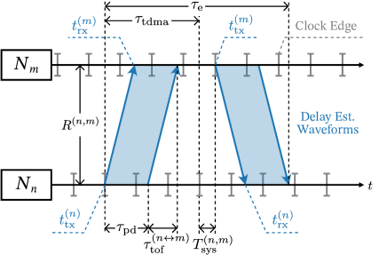
Figure 5: twtt diagram using a tdma scheme showing a single synchronization epoch. In this channel multiplexing scheme, each node has a scheduled transmission time separated by $\tau_{\mathrm{tdma}}$. The internode range $R^{(n,m)}$ and relative time error $\delta T_{\mathrm{sys}}^{(n,m)}$ are shown as quasi-static over the duration of the epoch; thus, $\tau_{\mathrm{tof}}^{(n\leftrightarrow m)}$ is also reciprocal and quasi-static during the epoch. Due to synchronization errors, node $N_{m}$ transmits its message slightly misaligned with the start of its tdma frame.

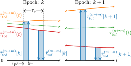
Figure 6: Apparent tof diagram for the twtt process. The nonlinearities in the $\bar{\tau}_{\mathrm{tof}}$ traces are magnified for illustration purposes, but care should be taken to ensure that $\tau_{\mathrm{e}}$ is short enough that the apparent tof between nodes is quasi-static during the synchronization epoch duration to ensure the assumption of channel reciprocity during the twtt exchange is not violated.

In this work we utilize the high-accuracy twtt methods described in [42], shown graphically in Figs. 5 and 6. This process uses a traditional twtt process to estimate the time offsets between the system clocks on each platform [52, 53, 54]; however, this process is limited to the accuracy of the time of transmission and arrival estimates from each sdr. On the transmit side, the radio transmit time can be scheduled to align with a clock edge relative to the system time; the dac and rfe do not appreciably increase the jitter, so the time of transmission can often be estimated with high certainty. Estimation of the toa is more challenging because the received waveform can arrive at any point between clock edges; thus, waveform optimization and toa refinement based on  [42] is performed to achieve high-accuracy time estimation using two-tone waveforms by leveraging the cooperative nature of the system.

III-A1 Two-Way Time Transfer

The goal of the twtt process is to estimate the accumulated clock phase error between the reference oscillators at each sdr. Using (4) and (6) we can define the time at the data converters as $T_{\mathrm{dac}}(t)$ and $T_{\mathrm{adc}}(t)$ from which we can define the apparent tof between nodes $N_{n}$ and $N_{m}$ during the $k$th synchronization epoch

$$\begin{split}\bar{\tau}_{\mathrm{tof}}^{(n\rightarrow m)}[k]&=T_{\mathrm{adc}}^{(m)}\!\left(t_{\mathrm{rx}}^{(m)}[k]\right)-T_{\mathrm{dac}}^{(n)}\!\left(t_{\mathrm{tx}}^{(n)}[k]\right)\end{split}$$ (16)

where $t_{\mathrm{tx}}^{(n)}[k]$ and $t_{\mathrm{rx}}^{(m)}[k]$ are the actual times that the waveforms were transmitted and received at nodes $N_{n}$ and $N_{m}$, respectively. Letting $t_{\mathrm{rx}}^{(m)}[k]=t_{\mathrm{tx}}^{(n)}[k]+\tau_{\mathrm{tof}}^{(n\rightarrow m)}[k]$ where $\tau_{\mathrm{tof}}^{(n\rightarrow m)}[k]$ is the true tof between nodes $N_{n}$ and $N_{m}$ and assuming a static phase calibration has been performed at each radio eliminating the static time errors at the data converters $\left(\text{i.e., }T_{\mathrm{0,dac}}^{(n,m)}=T_{\mathrm{0,adc}}^{(n,m)}=0\right)$, allows simplification to only terms of $T_{\mathrm{sys}}(t)$ at each node

$$\begin{split}\bar{\tau}_{\mathrm{tof}}^{(n\rightarrow m)}[k]&=T_{\mathrm{sys}}^{(m)}\!\left(t_{\mathrm{tx}}^{(n)}[k]+\tau_{\mathrm{tof}}^{(n\rightarrow m)}[k]\right)-T_{\mathrm{sys}}^{(n)}\!\left(t_{\mathrm{tx}}^{(n)}[k]\right)\\ &=\tau_{\mathrm{tof}}^{(n\rightarrow m)}[k]\left(1+\Delta f_{\mathrm{osc}}^{(m)}\right)+T_{\mathrm{0,sys}}^{(n,m)}\\ &\quad+\Delta f_{\mathrm{osc}}^{(n,m)}t_{\mathrm{tx}}^{(n)}[k]+\frac{(\nu_{\mathrm{\phi,dac}}[k]+\nu_{\mathrm{\phi,adc}}[k])}{2\pi f_{\mathrm{0,sys}}}.\end{split}$$ (17)

The quantity $\bar{\tau}_{\mathrm{tof}}^{(n\rightarrow m)}[k]$ is referred to as the apparent tof because the time estimate is derived from the clock estimates including local clock error; the $\rightarrow$ notation in the superscript indicates that is may not be reciprocal. The time offsets between nodes can then be estimated by

$$\begin{split}\hat{T}_{\mathrm{}}^{(n,m)}[k]&=\frac{\bar{\tau}_{\mathrm{tof}}^{(n\rightarrow m)}[k]-\bar{\tau}_{\mathrm{tof}}^{(m\rightarrow n)}[k]}{2}\\ &=\frac{1}{2}\Delta f_{\mathrm{osc}}^{(n,m)}\left(\tau_{\mathrm{tof}}^{(n\leftrightarrow m)}[k]+t_{\mathrm{tx}}^{(n)}[k]+t_{\mathrm{tx}}^{(m)}[k]\right)\\ &\qquad+T_{\mathrm{0,sys}}^{(n,m)}+\frac{\sqrt{2}(\nu_{\mathrm{\phi,dac}}[k]+\nu_{\mathrm{\phi,adc}}[k])}{4\pi f_{\mathrm{0,sys}}}\end{split}$$ (18)

where $\tau_{\mathrm{tof}}^{(n\leftrightarrow m)}=\tau_{\mathrm{tof}}^{(n\rightarrow m)}=\tau_{\mathrm{tof}}^{(m\rightarrow n)}$ is the bidirectional tof, assuming the tof is quasi-static over the synchronization epoch $\tau_{\mathrm{e}}=\tau_{\mathrm{tof}}^{(n\leftrightarrow m)}+t_{\mathrm{tx}}^{(n,m)}+\tau_{\mathrm{pd}}$, where $\tau_{\mathrm{pd}}$ is the twtt message pulse duration. Once the system times are closely aligned, $t_{\mathrm{tx}}^{(m)}\approx t_{\mathrm{tx}}^{(n)}+\tau_{\mathrm{tdma}}$, where $\tau_{\mathrm{tdma}}$ is the tdma time slot duration (see Fig. 5), which simplifies (18) to

$$\begin{split}\hat{T}_{\mathrm{}}^{(n,m)}[k]&\approx\left(T_{\mathrm{0,sys}}^{(n,m)}+\Delta f_{\mathrm{osc}}^{(n,m)}t_{\mathrm{tx}}^{(n)}[k]\right)\\ &\quad+\frac{1}{2}\Delta f_{\mathrm{osc}}^{(n,m)}\left(\tau_{\mathrm{tof}}^{(n\leftrightarrow m)}+\tau_{\mathrm{tdma}}\right)+\nu_{\mathrm{\phi}}[k]\\ &\approx T_{\mathrm{sys}}^{(n,m)}[k]+\frac{1}{2}\Delta f_{\mathrm{osc}}^{(n,m)}\left(\tau_{\mathrm{tof}}^{(n\leftrightarrow m)}+\tau_{\mathrm{tdma}}\right)\\ &\quad+\nu_{\mathrm{\phi}}[k]\end{split}$$ (19)

where $\nu_{\mathrm{\phi}}[k]$ is the phase noise term in (18). Furthermore, if the product of $\Delta f_{\mathrm{osc}}^{(n,m)}\tau_{\mathrm{tof}}^{(n\leftrightarrow m)}$ is small relative to the level of accuracy required, it may be neglected (e.g., for oscillators with $\Delta f_{\mathrm{osc}}^{(n,m)}=6$ ppm over a 100 m channel, the error would be $\approx\,$1 ps). Similarly, if the tdma period is kept short and the product of $\Delta f_{\mathrm{osc}}^{(n,m)}\tau_{\mathrm{tdma}}$ is small, the impact of clock drift over the tdma window can also be neglected (e.g., for oscillators with $\Delta f_{\mathrm{osc}}^{(n,m)}=6$ ppm with $\tau_{\mathrm{tdma}}=$10\text{\,}\mathrm{\SIUnitSymbolMicro s}$$, the error would be $\approx\,$30 ps); acceptable levels of accuracy will be determined by the application. With these assumptions (18) becomes

$$\begin{split}\hat{T}^{(n,m)}[k]&\approx T_{\mathrm{sys}}^{(n,m)}[k]+\nu_{\mathrm{\phi}}[k]\end{split}$$ (20)

where $T_{\mathrm{sys}}^{(n,m)}$ is given by (13). From (18) it can also be seen that the time offset estimate does not depend on the path that the signal traversed between radios, meaning that the technique is robust to nlos scenarios, so long as the path taken is reciprocal [77].

In a similar way, the internode tof can be estimated by simply taking the average of the apparent tof

$$\begin{split}\hat{\tau}_{\mathrm{tof}}^{(n\leftrightarrow m)}[k]&=\frac{\bar{\tau}_{\mathrm{tof}}^{(n\rightarrow m)}[k]+\bar{\tau}_{\mathrm{tof}}^{(m\rightarrow n)}[k]}{2}\\ &=\tau_{\mathrm{tof}}^{(n\leftrightarrow m)}+\frac{1}{2}\tau_{\mathrm{tof}}^{(n\leftrightarrow m)}\left(\Delta f_{\mathrm{osc}}^{(n)}+\Delta f_{\mathrm{osc}}^{(m)}\right)\\ &\qquad-\frac{1}{2}\Delta f_{\mathrm{osc}}^{(n,m)}\tau_{\mathrm{tdma}}+\nu_{\mathrm{\phi}}[k]\end{split}$$ (21)

which, similar to the time offset estimation, the oscillator error term may be neglected if the product of the tof and average oscillator error is small or well synchronized (e.g., for oscillators with $\Delta f_{\mathrm{osc}}^{(n,m)}=6$ ppm over a 100 m channel, the error would be $\approx\,$1 ps, or $300\text{\,}\mathrm{\SIUnitSymbolMicro m}$). The tdma period may also be neglected if the product of $\Delta f_{\mathrm{osc}}^{(n,m)}\tau_{\mathrm{tdma}}$ is small (e.g., for oscillators with $\Delta f_{\mathrm{osc}}^{(n,m)}=6$ ppm with $\tau_{\mathrm{tdma}}=$10\text{\,}\mathrm{\SIUnitSymbolMicro s}$$, the error would be $\approx\,-$30 ps, or $-9\text{\,}\mathrm{mm}$)

$$\begin{split}\hat{\tau}_{\mathrm{tof}}^{(n\leftrightarrow m)}[k]\approx\tau_{\mathrm{tof}}^{(n\leftrightarrow m)}+\nu_{\mathrm{\phi}}[k].\end{split}$$ (22)

From the tof estimate, the internode range can be estimated directly by $\hat{R}^{(n\leftrightarrow m)}[k]=c\cdot\hat{\tau}_{\mathrm{tof}}^{(n\leftrightarrow m)}[k]$. It is worth noting here that (21) shows that accuracy depends not only on the relative internode frequency error as in (19), but also the mean frequency error of the system $\left(\Delta f_{\mathrm{osc}}^{(n)}+\Delta f_{\mathrm{osc}}^{(m)}\right)/2$. This is because the tof is relative to the frequency standard used by the system, i.e., if range in meters is desired, the timing deviation from the si definition of the second will result in additional ranging error. It is also important to note that the tof is not necessarily the shortest path between elements—typically the quantity that is desired for beamforming phase weighting computations—as it may be impacted by multipath or nlos. To an extent this may be mitigated in multipath scenarios by choosing a waveform with high occupied bandwidth to resolve multipath scattering; however, this is not always feasible and, as will be discussed in Section III-A2 increases the lower-bound on toa estimation variance relative to a sparse waveform with low occupied bandwidth (i.e., low spectral occupancy relative to the maximum spectral extent of the waveform).

III-A2 High-Accuracy toa Estimation

To achieve high-accuracy toa estimation, the waveform is first optimized to minimize the time estimation variance lower bound for a given bandwidth by studying the crlb for toa estimation, then a multi-step time estimation refinement process is implemented to estimate the delay to below a single clock tick on the adc using matched filtering, qls peak refinement, and a lut to remove residual bias due to qls by leveraging the cooperative nature of the system.

In the twtt exchange, a narrowband received signal at the rf port $s_{\mathrm{rx}}^{(n)}(t)$ can be modeled as a time delayed and frequency shifted copy of $s_{\mathrm{tx}}^{(m)}(t)$ with added noise

$$s_{\mathrm{adc}}^{(m)}(t)=\alpha s_{\mathrm{tx}}^{(n)}\!\left(t-\bar{\tau}_{\mathrm{tof}}^{(n\rightarrow m)}\right)\exp{\left(j2\pi\bar{f}_{d}^{(n,m)}t\right)}+w(t)$$ (23)

where $\alpha$ is a complex channel weight describing the phase shift due to propagation delay and amplitude scaling due to channel loss and $w(t)$ is a white Gaussian noise process with a psd of $\nu_{0}/2$ due to timing phase noises and thermal noise. The lower bound on apparent time delay and apparent Doppler shift can then be found by solving the crlb inequality with respect to each parameter resulting in [78, §6.3][79, 80]

$$\mathrm{var}\!\left(\hat{\bar{\tau}}^{(n\rightarrow m)}_{\mathrm{tof}}-\bar{\tau}^{(n\rightarrow m)}_{\mathrm{tof}}\right)\geq\frac{\nu_{0}}{2|\alpha|^{2}}\left(\zeta_{f}^{2}-\frac{1}{E_{s}}\mu_{f}^{2}\right)^{-1}$$ (24)

where $|\alpha|^{2}/\nu_{0}$ is the post-integration snr, $E_{s}\triangleq\int|s_{\mathrm{tx}}(t)|^{2}\,\mathrm{d}t$ is the total signal energy, $\zeta_{f}^{2}\triangleq\int(2\pi f)^{2}|S_{\mathrm{tx}}(f)|^{2}\,\mathrm{d}f$ is the mean-square bandwidth, and $\mu_{f}\triangleq\int 2\pi f|S_{\mathrm{tx}}(f)|^{2}\,\mathrm{d}f$ is the mean frequency. The apparent Doppler shift is

$$\mathrm{var}\!\left(\hat{\bar{f}}^{(n,m)}_{d}-\bar{f}^{(n,m)}_{d}\right)\geq\frac{\nu_{0}}{2|\alpha|^{2}}\left(\zeta_{t}^{2}-\frac{1}{E_{s}}\mu_{t}^{2}\right)^{-1}$$ (25)

where $\zeta_{t}^{2}\triangleq\int(2\pi t)^{2}|s_{\mathrm{tx}}(t)|^{2}\,\mathrm{d}t$ is the mean-square duration, and $\mu_{t}^{2}\triangleq\int 2\pi t|s_{\mathrm{tx}}(t)|^{2}\,\mathrm{d}t$ is the mean time. For signals centered around dc, the mean frequency can be omitted; similarly, by choosing a time reference at the center of the waveform, the mean time may also be omitted. The two-way accuracy bound for both the time error and tof may then be obtained simply by taking the average of the variances of the one-way tof estimate

$$\begin{multlined}\mathrm{var}\!\left(\hat{T}_{\mathrm{}}^{(n,m)}-{T}_{\mathrm{}}^{(n,m)}\right)\\ \geq\frac{1}{2}\bigg{[}\mathrm{var}\!\left(\hat{\bar{\tau}}^{(n\rightarrow m)}_{\mathrm{tof}}-\bar{\tau}^{(n\rightarrow m)}_{\mathrm{tof}}\right)+\mathrm{var}\!\left(\hat{\bar{\tau}}^{(m\rightarrow n)}_{\mathrm{tof}}-\bar{\tau}^{(m\rightarrow n)}_{\mathrm{tof}}\right)\bigg{]}\end{multlined}\mathrm{var}\!\left(\hat{T}_{\mathrm{}}^{(n,m)}-{T}_{\mathrm{}}^{(n,m)}\right)\\ \geq\frac{1}{2}\bigg{[}\mathrm{var}\!\left(\hat{\bar{\tau}}^{(n\rightarrow m)}_{\mathrm{tof}}-\bar{\tau}^{(n\rightarrow m)}_{\mathrm{tof}}\right)+\mathrm{var}\!\left(\hat{\bar{\tau}}^{(m\rightarrow n)}_{\mathrm{tof}}-\bar{\tau}^{(m\rightarrow n)}_{\mathrm{tof}}\right)\bigg{]}$$ (28)

which implies, given identical waveforms in both directions of the twtt exchange, the two-way accuracy is inversely proportional to the average snr seen at each receiver.

From (24) and (25) it is evident that lower bound on variance of both time and frequency estimation is inversely proportional to snr at the receiver. However, in (24) the signal is also proportional to the inverse of the mean-square bandwidth $\zeta_{f}^{2}$ which is maximized by moving all of the energy of the frequency spectrum to the edges of the available bandwidth, e.g., two infinite duration tones separated by maximum available bandwidth; in (25) the signal is also inversely proportional the mean-square duration $\zeta_{t}^{2}$ which is maximized by placing all of the signal energy at the edges of the available pulse duration, e.g., two infinite bandwidth pulses at the edges of the pulse duration. This leads to conflicting requirements, thus making it impossible to simultaneously minimize both instantaneous toa estimation and instantaneous frequency offset estimation. In this work, we choose to achieve the highest available instantaneous estimation of the relative clock phase error between systems (fast-time) and derive the frequency error from sequential estimates of time (slow-time); we utilize a ptt waveform which approximates placing the signal energy at the edges of the available bandwidth in fast-time, and over long time intervals we will obtain relatively short duration pulses separated by a large duration of time, approximating the optimal frequency estimation technique of widely separated impulses in time.

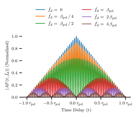
Figure 7: Ambiguity function slices of constant apparent Doppler shift $\bar{f}_{d}$ given by (30) with ptt separation $\beta_{\mathrm{ptt}}=30/\tau_{\mathrm{pd}}$ and pulse bandwidth $\beta_{\mathrm{pd}}=1/\tau_{\mathrm{pd}}$. Several slices are plotted showing that as $\bar{f}_{d}$ approaches $\beta_{\mathrm{pd}}/2$, the peak of the magnitude of the matched filter no longer corresponds to the zero-delay lobe meaning a simple peak find can no longer be used.

The ptt waveform is ideally described by

$$s(t)=\Pi\!\left(\frac{t}{\tau_{\mathrm{pd}}}\right)\left(e^{-j\pi\beta_{\mathrm{ptt}}t}+e^{j\pi\beta_{\mathrm{ptt}}t}\right)$$ (29)

where $\Pi(t/\tau_{\mathrm{pd}})$ is a rectangular windowing function with a duration $\tau_{\mathrm{pd}}$ and $\beta_{\mathrm{ptt}}=f_{2}-f_{1}$ is the tone separation, assumed to be centered about dc after downconversion and sampling. The half-power bandwidth of each tone due to the rectangular pulse duration is $\beta_{\mathrm{pd}}=1/\tau_{\mathrm{pd}}$. For a ptt waveform $\zeta_{\mathrm{f(ptt)}}=\pi\beta_{\mathrm{ptt}}$ and $\zeta_{\mathrm{t(ptt)}}=\pi\tau_{\mathrm{pd}}/\sqrt{3}$ [80].

To perform toa estimation a matched filter is formulated which maximizes the snr in the presence of additive white gaussian noise, which is simply the convolution of the received waveform with the complex conjugate of the transmitted waveform [81, §4.2]. However, the impact of frequency error between the matched filter and the received waveform causes a distortion in the ideal matched filter. The impact of time and frequency offsets due to $\bar{\tau}_{\mathrm{tof}}^{(n\rightarrow m)}$ and $\bar{f}_{d}^{(n,m)}$ on the matched filter is given by its ambiguity function [82]

$$\begin{split}&\left|\mathrm{AF}(t,\bar{f}_{d})\right|=\left|\int_{-\infty}^{\infty}s^{*}(\tau-t)s(\tau)e^{j2\pi\bar{f}_{d}\tau}d\tau\right|\\ &\begin{multlined}=\Bigg{|}\frac{e^{j\pi\bar{f}_{d}t}}{4}\Lambda\!\left(\frac{t}{\tau_{\mathrm{pd}}}\right)\Bigg{\{}\left(e^{-j\pi\beta_{\mathrm{ptt}}t}+e^{j\pi\beta_{\mathrm{ptt}}t}\right)\\ \times\operatorname{sinc}\left[\pi\bar{f}_{d}\Lambda\!\left(\frac{t}{\tau_{\mathrm{pd}}}\right)\right]+\operatorname{sinc}\!\left[\pi(\beta_{\mathrm{ptt}}+\bar{f}_{d})\Lambda\!\left(\frac{t}{\tau_{\mathrm{pd}}}\right)\right]\\ \qquad\qquad+\operatorname{sinc}\!\left[\pi(\bar{f}_{d}-B_{\mathrm{tt}})\Lambda\!\left(\frac{t}{\tau_{\mathrm{pd}}}\right)\right]\Bigg{\}}\Bigg{|}\end{multlined}=\Bigg{|}\frac{e^{j\pi\bar{f}_{d}t}}{4}\Lambda\!\left(\frac{t}{\tau_{\mathrm{pd}}}\right)\Bigg{\{}\left(e^{-j\pi\beta_{\mathrm{ptt}}t}+e^{j\pi\beta_{\mathrm{ptt}}t}\right)\\ \times\operatorname{sinc}\left[\pi\bar{f}_{d}\Lambda\!\left(\frac{t}{\tau_{\mathrm{pd}}}\right)\right]+\operatorname{sinc}\!\left[\pi(\beta_{\mathrm{ptt}}+\bar{f}_{d})\Lambda\!\left(\frac{t}{\tau_{\mathrm{pd}}}\right)\right]\\ \qquad\qquad+\operatorname{sinc}\!\left[\pi(\bar{f}_{d}-B_{\mathrm{tt}})\Lambda\!\left(\frac{t}{\tau_{\mathrm{pd}}}\right)\right]\Bigg{\}}\Bigg{|}\end{split}$$ (30)

where $\Lambda\!\left(t/\tau_{\mathrm{pd}}\right)$ is a triangular amplitude windowing function of duration $2\tau_{\mathrm{pd}}$. Slices of the normalized ambiguity function are plotted in Fig. 7 using the default parameters used in the experiments in this work. By looking at the zero-Doppler cut $\bar{f}_{d}=0$ of the ambiguity function, the periodic structure of the matched filter response to the ptt waveform can be seen which includes a triangular envelope due to the convolution of the rectangular pulse envelope modulated by a periodic structure whose periodicity is equal to the inverse of the beat frequency between tone carriers $1/\beta_{\mathrm{ptt}}$; due to this fact, the ptt waveform is not used for radar ranging as the sidelobes would significantly degrade image quality in any complex scene; however, in a cooperative two-way system, this waveform can be used so long as the pulse waveforms do not overlap in time, frequency, and space. Along the zero-delay cut $t=0$ a sinc shape is produced due to the rectangular pulse modulation envelope in the frequency domain. Of significant interest is the fact that the triangular shape of the matched filter begins to flatten out under moderate apparent Doppler shifts, meaning that the ability to pick the correct peak using a simple peak-finding operation decreases under noise; furthermore, at a certain frequency error, the peak of the matched filter no longer represents the true time delay at all. This cross-over point appears at $\bar{f}_{d}=1/(2\tau_{\mathrm{pd}})$, meaning a simple peak find will no longer yield the correct delay if the apparent Doppler shift is greater than half the pulse bandwidth, shown in green in Fig. 7; practically, a larger margin will be required due to added noise which can cause amplitude fluctuations in the $1/\beta_{\mathrm{ptt}}$ lobes of the matched filter. Generally, this implies that shorter pulses will be more resilient to frequency offset and Doppler shift. This conflicts with the crlb for toa estimation described in (24); thus, a balance in ptt duration must be made between minimizing time estimation ability and resilience to frequency offset and Doppler shift which will be dependent on the application.

While the matched filtering process produces a waveform at its output that, under small to moderate apparent Doppler shifts, maximizes the output power at the true time delay of the waveform, it is still discretized to the sampling period of the platform which, for non-rf sampling sdr, is significantly larger than the rf carrier period. Therefore, to be able to adequately correct for the carrier phase, a further time estimation refinement process must be employed. Typically, the matched filter is employed in the frequency domain as $s_{\mathrm{mf}}(t)=\mathcal{F}^{-1}\{\mathcal{F}[s_{\mathrm{rx}}(t)]\mathcal{F}[s_{\mathrm{tx}}^{*}(t)]\}$ to achieve a complexity of $\mathcal{O}(N\log N)$ as opposed to the $\mathcal{O}(N^{2})$ required for direct convolution for an $N$-sample waveform; in this case, a zero-padding factor of $M$ may be performed on the frequency domain representation prior to the ift which acts as an unbiased interpolation, but comes at the cost of increasing the computational complexity to $\mathcal{O}(MN\log(MN))$. To achieve high levels of interpolation using this technique, the computational load becomes intractable for real-time operation. Thus, an alternative method must be used. Many other highly performant options exist which attempt to estimate the true time delay by using a regression model to fit a curve to the sampled matched filter data such as qls [83] [81, §7.2], sinc-ls [1], and mf-ls [84]. While mf-ls theoretically provides an unbiased peak estimate by performing regression of the matched filter magnitude itself, it requires iterative computation of the matched filter which is typically computationally expensive, making it challenging to implement for latency-sensitive operations such as time and frequency correction. The sinc-ls operation provides an appropriate curve fit for matched filters with a sinc-like shape such as lfm waveforms, but is generally an iterative process, though it is noted in [1] that a closed form solution is available for three sample points. The qls toa correction estimation is simple and also has a known closed form solution using three sample points [81, §7.2]. For a signal whose true time delay is $\tau_{\mathrm{d}}$ and discrete-time matched filter is $s_{\mathrm{mf}}[i]$ where $i$ is the sample index, the qls process begins with an initial time estimate given simply by the peak-find result of the matched filter $i_{\mathrm{max}}=\mathrm{argmax}_{i\in\{0\dots 2L-1\}}s_{\mathrm{mf}}[i]$ for a signal of length $L$, yielding the initial time estimate of $\hat{\tau}=i_{\mathrm{max}}/T_{\mathrm{s,adc}}$. The result is then refined by computing the centroid of a parabola fit through $i_{\mathrm{max}}$ and its two adjacent sample points

$$\begin{split}\hat{\tau}^{\prime}=\frac{T_{\mathrm{s,adc}}}{2}\frac{s_{\mathrm{mf}}[i_{\mathrm{max}}-1]-s_{\mathrm{mf}}[i_{\mathrm{max}}+1]}{s_{\mathrm{mf}}[i_{\mathrm{max}}-1]-2s_{\mathrm{mf}}[i_{\mathrm{max}}]+s_{\mathrm{mf}}[i_{\mathrm{max}}+1]}\end{split}.$$ (31)

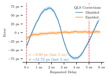
Figure 8: Time delay estimation error with and without qls bias correction lut applied. In this scenario a ptt waveform with $\beta_{\mathrm{ptt}}=\;$$40\text{\,}\mathrm{MHz}$ was transmitted from one channel and received at another on an Ettus X310 sdr and sampled at 200 MSa/s while the transmitted waveform was digitally delayed. Red dashed lines indicate one sample period on the adc. The slight upward trend at the start is due to device warm-up after starting; this trend disappears after several minutes of operation.

The qls refinement value is then added to the original estimate to refine its value $\hat{\tau}_{\mathrm{qls}}=\hat{\tau}+\hat{\tau}^{\prime}$. Because the shape of the quadratic does not exactly match that of the matched filter, some small amount of bias is introduced in the estimate, shown experimentally in Fig. 8; however, it is observed that this bias trend is a function only of the adc sample rate and waveform parameters. Because of the cooperative nature of the system, these parameters are both known a priori allowing a lut $\tau^{\prime\prime}(\tau^{\prime})$ to be computed and used to correct for the residual qls error as $\hat{\tau}_{\mathrm{qls,lut}}=\hat{\tau}+\hat{\tau}^{\prime}+\hat{\tau}^{\prime\prime}$. While computing the lookup table can be slow for very fine time steps, indexing into the lut can be performed very quickly at runtime, and a simple linear interpolation between lut can be applied to minimize residual error [42].

III-B Frequency Estimation

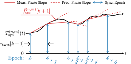
Figure 9: Frequency offset estimation process. The time transfer processes may be either uniformly sampled or arbitrarily sampled as is shown in this figure. Clock noise is shown magnified to highlight the process; in practice, the spacing between twtt processes should be small enough that the clock drift is approximately linear.

The relative frequency error can be estimated to first order as the relative phase drift divided by observation interval measured at some node $n$. As established in (6), time and phase are related by the nominal frequency; thus, this can be accomplished directly by estimating the clock time offsets by using the high accuracy time estimation described in Section III-A, shown in Fig. 9. From this, the dimensionless frequency difference between platforms can be estimated by

$$\begin{split}\Delta\hat{f}_{\mathrm{osc}}^{(n,m)}[k]=\frac{\hat{T}_{\mathrm{sys}}^{(n,m)}[k]-\hat{T}_{\mathrm{sys}}^{(n,m)}[k-1]}{\tau_{\mathrm{twtt}}[k]}\end{split}$$ (32)

where $\tau_{\mathrm{twtt}}[k]=t_{\mathrm{tx}}^{(n)}[k]-t_{\mathrm{tx}}^{(n)}[k-1]$. In a similar manner, the relative radial velocity could be estimated by the internode position change versus time $\hat{v}_{r}=\mathrm{d}R^{(n,m)}/\mathrm{dt}$, assuming a los path. Using this technique, the crlb on frequency estimation can be approximated by (25) with $\zeta_{t}=\pi\tau_{\mathrm{twtt}}[k]$ where $\tau_{\mathrm{twtt}}[k]$ is the true time duration between the start of each synchronization epoch, assuming $\tau_{\mathrm{twtt}}[k]\gg\tau_{\mathrm{pd}}$; however, in practice, a more accurate estimate of performance can be found in a manner similar to (28)

$$\begin{multlined}\mathrm{var}\!\left({\hat{f}}_{\mathrm{osc}}^{(n,m)}[k]-f_{\mathrm{osc}}^{(n,m)}[k]\right)\\ \geq\frac{1}{2\tau_{\mathrm{twtt}}[k]}\bigg{[}\mathrm{var}\!\left(\hat{T}_{\mathrm{}}^{(n,m)}[k-1]-{T}_{\mathrm{}}^{(n,m)}[k-1]\right)\\ +\mathrm{var}\!\left(\hat{T}_{\mathrm{}}^{(n,m)}[k]-{T}_{\mathrm{}}^{(n,m)}[k]\right)\bigg{]}\end{multlined}\mathrm{var}\!\left({\hat{f}}_{\mathrm{osc}}^{(n,m)}[k]-f_{\mathrm{osc}}^{(n,m)}[k]\right)\\ \geq\frac{1}{2\tau_{\mathrm{twtt}}[k]}\bigg{[}\mathrm{var}\!\left(\hat{T}_{\mathrm{}}^{(n,m)}[k-1]-{T}_{\mathrm{}}^{(n,m)}[k-1]\right)\\ +\mathrm{var}\!\left(\hat{T}_{\mathrm{}}^{(n,m)}[k]-{T}_{\mathrm{}}^{(n,m)}[k]\right)\bigg{]}$$ (36)

where the frequency estimation variance is inversely proportional to the time between observations and the average snr of all four received waveforms, assuming the waveform parameters are held constant.

Because this technique is periodic, its accuracy will be limited by the power spectral density profile of the apparent Doppler shift, i.e., the power spectral density of platform vibrations and phase noise of the system, which have been studied in[85] and [86] for periodically synchronized systems. Critically, the update rate must be significantly greater than the frequencies in which most of the power spectrum area exists to achieve a high level of coordination.

IV Direct Phase Compensation

The uncompensated waveforms transmitted and received at node $N_{n}$ are given by (8) and (10). To compensate these waveforms, the phase error imparted by the initial time offset of the system clock $T_{\mathrm{0,sys}}^{\mathrm{(n)}}$, transmitter phase delay $\phi_{\mathrm{0,tx}}^{(n)}$, and reference oscillator frequency offset $\delta f_{\mathrm{osc}}^{(n)}(t)$ which imparts both a cfo and sfo, need to be corrected. This can be accomplished in two steps:

1. modify the sampling time of the baseband waveform to correct the relative sampling time offset

   $$\tilde{\Psi}(t_{s}[i])=h\!\left(\Psi\!\left(t_{s}[i]\right);t_{s}[i]+T_{\mathrm{sys}}^{(n,m)}(t_{s}[i])\right)$$ (37)

   where $h(x;t)$ is an arbitrary time resampling function and $\Psi(t)$ is the baseband transmit or receive waveform, and

2. modulate the baseband waveform with a phase $\tilde{\phi}_{\mathrm{lo}}(t)$ opposite that of the time-varying relative internode carrier phase offsets.

Using the linear frequency drift model, the carrier phase compensation applied at node $N_{n}$ is the opposite of (12)

$$\begin{split}\tilde{\phi}_{\mathrm{lo}}^{(n)}(t)&=-\phi_{\mathrm{lo}}^{(n,m)}(t_{s}[i])\\ &=-2\pi f_{\mathrm{0,lo}}^{(n)}\Delta f_{\mathrm{osc}}^{(n,m)}t_{s}[i]-\phi_{\mathrm{0,lo}}^{(n,m)}.\end{split}$$ (38)

Because the analytic representation of the waveform $\Psi_{\mathrm{tx}}(t)$ is available at the transmitter, the underlying waveform can be directly sampled at arbitrary times, making no assumptions on the system dynamics model used; thus, the compensated transmit waveform at baseband at node $N_{n}$ is

$$\begin{split}\begin{multlined}\tilde{\Psi}_{\mathrm{tx}}^{(n)}[i]=\Psi_{\mathrm{tx}}\!\left(t_{s}[i]+T_{\mathrm{sys}}^{(n,m)}(t_{s}[i])\right)\\ \exp{-j\left[2\pi f_{\mathrm{0,lo}}^{(m)}\Delta f_{\mathrm{osc}}^{(n,m)}t_{s}[i]+\phi_{\mathrm{0,tx}}^{(n,m)}\right]}\end{multlined}\tilde{\Psi}_{\mathrm{tx}}^{(n)}[i]=\Psi_{\mathrm{tx}}\!\left(t_{s}[i]+T_{\mathrm{sys}}^{(n,m)}(t_{s}[i])\right)\\ \exp{-j\left[2\pi f_{\mathrm{0,lo}}^{(m)}\Delta f_{\mathrm{osc}}^{(n,m)}t_{s}[i]+\phi_{\mathrm{0,tx}}^{(n,m)}\right]}\end{split}$$ (39)

which, once transmitted, will cancel the time and phase offsets of the transmitter. The compensation on the received waveform is more challenging due to the fact that there is no analytic representation available of $s_{\mathrm{adc}}(t)$ and thus the sampled waveform must be arbitrarily resampled to correct for sfo. This can be modeled by

$$\begin{multlined}\tilde{\Psi}_{\mathrm{rx}}^{(m)}[i]=h\!\left(\Psi_{\mathrm{rx}}\!\left(t_{s}[i]\right);t_{s}[i]+T_{\mathrm{sys}}^{(n,m)}(t_{s}[i])\right)\\ \exp{j\left[2\pi f_{\mathrm{0,lo}}^{(m)}\Delta f_{\mathrm{osc}}^{(n,m)}t_{s}[i]+\phi_{\mathrm{0,lo}}^{(n,m)}\right]}\end{multlined}\tilde{\Psi}_{\mathrm{rx}}^{(m)}[i]=h\!\left(\Psi_{\mathrm{rx}}\!\left(t_{s}[i]\right);t_{s}[i]+T_{\mathrm{sys}}^{(n,m)}(t_{s}[i])\right)\\ \exp{j\left[2\pi f_{\mathrm{0,lo}}^{(m)}\Delta f_{\mathrm{osc}}^{(n,m)}t_{s}[i]+\phi_{\mathrm{0,lo}}^{(n,m)}\right]}$$ (42)

noting that the carrier phase modulation is the conjugate of that applied on the transmit side. Further challenging the receive-side sampling time compensation is the fact that truly arbitrary time resampling techniques, such as Lanczos resampling [87], are generally computationally expensive compared to simple constant time fractional delays filters, or constant frequency offset multirate filters [88]. However, the complexity of the receive-side sampling time compensation required is dictated by the tbp of the incoming waveform. For long, wideband incoming waveforms, accurate compensation is necessary to ensure coherence, while for short duration and or narrowband pulses, only a constant fractional time delay may be required. This can be formulated in terms of a maximum tolerable phase error at the end of a pulse duration. In the case of the linear frequency drift model, a constant phase delay error model can be described as

$$\epsilon_{\mathrm{\phi}}=\Delta f\cdot\mathrm{TBP}$$ (43)

where $\Delta f$ is the dimensionless relative frequency error and TBP is the product of the incoming waveform duration and its bandwidth (i.e., the time-bandwidth product). The maximum tolerable $\epsilon_{\mathrm{\phi}}$ will depend heavily on the application. As an example, in the case of twtt, the frequency error of the incoming waveform will impact the matched filter response, as shown by the ambiguity function in Fig. 7, given by (30), if the total frequency error is less than $\beta_{\mathrm{pd}}/2$, the peak find will still obtain the correct time result in a noise-free scenario; in this case, the incoming waveform may not need to be resampled, instead only the final toa estimate may be compensated, saving significant computation time. In this work, the system has typical internode frequency errors of $\Delta f<$ 1 ppm and the waveform used has a tbp $=30$ yielding $\epsilon_{\phi}=$ $1.8\text{\,}\mathrm{m\SIUnitSymbolDegree}$ of accumulated phase error, thus having little impact on the performance.

V Wireless Coordination Experiments

V-A Hardware Configuration

The wireless coordination experiments consisted of three different hardware configurations. In all three configurations, each node consisted of an Ettus Research X310 usrp connected to a Dell Optiplex 7080 host with an Intel i7-10700 and 16 GB of DDR4 memory connected via 10 Gigabit Ethernet (GbE). The hosts were connected via 1 GbE to a central network switch for digital communication between nodes. The radios on each node utilized channel A to perform twtt for time and frequency offset estimation; the first and last nodes in the array (node $N_{0}$ and $N_{1}$) contained an external Mini-Circuits ZFSWA2R-63DR+ antenna diversity switch to multiplex between a twtt antenna, and a “beamforming” cable connected to an oscilloscope to directly measure beamforming signals from each node at an independent external observer to characterize expected real-world beamforming performance parameters and isolate time, frequency, and phase performance of each node. The twtt antenna used in all experiments was a Taoglas TG.56.8113 wideband monopole. In all configurations, the antenna on node $N_{0}$ was affixed to a motorized linear actuator. In static configurations, the antenna $N_{0}$ was held fixed at a distance of $\sim$$1\text{\,}\mathrm{m}$ from antenna $N_{1}$; in dynamic experiments the internode distance between $N_{0}$ and $N_{1}$ varied from $37\text{\,}\mathrm{cm}$ to $134\text{\,}\mathrm{cm}$, spanning $\sim$$1\text{\,}\mathrm{m}$. The three hardware configurations were designated Configuration A through Configuration C.

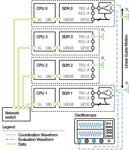
Figure 10: Configuration A: Fully-digital wireless time and frequency coordination. Number of nodes was varied between 2 and 4 in various experiments. In all experiments, nodes $N_{0}$ and $N_{1}$ were connected to the oscilloscope; due to the largest tdma time separation and largest internode distance, this evaluates the worst-case synchronization performance in the array.

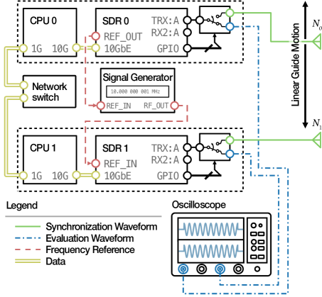
Figure 11: Configuration B: Fully-digital time and frequency coordination with a known static relative frequency offset via signal generator. In this experiment, the frequency offset estimation accuracy is evaluated using the known frequency error introduced by the signal generator.

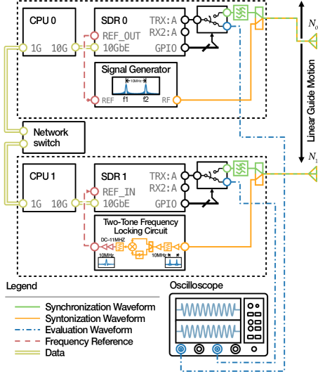
Figure 12: Configuration C: Fully-digital time coordination with analog continuous wireless frequency transfer based on [42].

• Configuration A (Fig. 10) was configured to run using the fully wireless digital time-frequency coordination procedure described in this paper with varying parameters. Parameters evaluated were snr, pulse duration $\tau_{\mathrm{pd}}$, epoch duration $\tau_{e}$, average resynchronization interval $\tau_{\mathrm{twtt}}$, and node scaling from 2–4 nodes under static and dynamic cases.

• Configuration B (Fig. 11) evaluated the ability of the system to estimate and correct for a known fixed frequency offset. This configuration added a fixed frequency offset between nodes $N_{0}$ and $N_{1}$ by using the $10\text{\,}\mathrm{MHz}$ frequency reference from the sdr of node $N_{0}$ to discipline a Keysight N5183A MXG signal generator signal generator which was used to generate a reference signal with a known frequency error which was provided to the $10\text{\,}\mathrm{MHz}$ frequency reference input on the sdr of node $N_{1}$. Because the oscillator noise is no longer independent between nodes, this allows a more accurate lower bound of the estimator accuracy for the system to be evaluated under a known frequency offset, independent of system oscillator drifts.

• Configuration C (Fig. 12) evaluated the performance of the system compared with the two-tone cw analog wireless frequency transfer technique used in [42, 36, 41] under relative motion with varying velocities. A Keysight E8267D PSG signal generator disciplined by the reference oscillator on sdr 0 was used to transmit the cwtt frequency reference. In this configuration, the frequency transfer is handled entirely via the analog system, and thus the sdr digital rf system is only used for time and range estimation. Because the frequency transfer circuit directly disciplines the SYS PLL in this scenario, the phase will also change based on the tof between the transmitting and receiving nodes. To correct for this phase rotation, the twtt estimate is used to apply an additional compensation phase in this configuration.

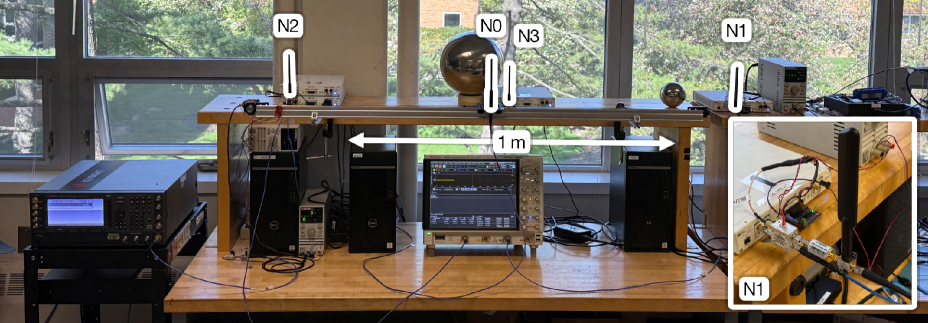
Figure 13: Photograph of the experimental configuration. Nodes were numbered $N_{0}$ through $N_{3}$; nodes $N_{0}$ and $N_{1}$ were always connected to the oscilloscope to measure beamforming performance.

In Configuration A, a Keysight DSOS8404A oscilloscope was used, and in Configuration B and Configuration C, a Keysight MSOX92004A oscilloscope was used. A photograph of the experimental setup is show in Fig. 13. Large metallic spheres in addition to the cement pillar and metal window frames were used to induce significant multipath reflections into the system to demonstrate the robustness to time-varying multipath channels.

V-B Software Configuration

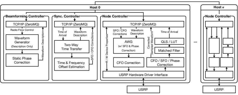
Figure 14: Software flow graph. Software utilized a centralized topology where Host 0 is running the Synchronization Controller and Beamforming Controller to orchestrate their respective tasks, with distributed signal processing taking place on each node in the Node Controllers. Each node ran a Node Controller which brokers access to the usrp resource and performs on-node waveform sampling, phase–frequency correction, and toa estimation via matched filter and qls. Interprocess and internode communication utilized ZeroMQ over TCP/IP.

The software was developed using usrp Hardware Driver (UHD) 4.8 and GNU Radio 3.10 and ran on Ubuntu 24.04. The software was separated logically into three separate programs termed controllers shown schematically in Fig. 14. In this system, each controller was a GNU Radio flow graph. The blocks in each flow graph were primarily written using Python 3.12, making extensive use of NumPy [89] and Numba [90] to achieve high performance, with only data manipulation blocks written in C++.

• Node Controller: This controller acts as the primary arbitrator between other array controllers and the usrp resource. It interprets waveform description dictionaries and samples the waveform on-device in an awg block, using the known sampling time offsets and applies a beat frequency to compensate for the lo frequency error, as described by (39). On the receive side it performs cfo, sfo, and phase corrections, as needed, described by (42); in these experiments the sfo was not enabled on receive due to the minimal amount of error in the twtt messages, as described by (43) in Section IV. Finally, this controller also handles the toa estimation by performing the matched filter and qls–lut refinement process required for high-accuracy twtt, described in Section III-A2, distributing the processing across nodes and performing data compression so only the timestamps must be transmitted between nodes.

• Synchronization Controller: This controller performs the twtt process described in Section III-A1 by orchestrating the Node Controllers to transmit twtt waveforms at known times and collecting their refined toa estimates; these estimates are then used to compute the frequency offsets using the techniques described in Section III-B.

• Beamforming Controller: This controller generates the evaluation pulses that are sent to the oscilloscope to verify system performance.

Within each GNU Radio flow graph, interprocess communication was accomplished using the message passing interface instead of the streaming interface to reduce latency at the expense of overall computational bandwidth; similarly, the radios were operated via UHD in a “bursty” mode, using finite duration pre-scheduled timed transmit and receive commands to ensure the exact transmit and receive times are known including host to radio transport latency. Between each of the controllers, communication was accomplished using ZeroMQ via TCP/IP to scale the distributed computing model easily between hosts. In this system the Beamforming and Synchronization controllers are centralized and are run on host 0 in a centralized manner; however, it should be noted that decentralized time and frequency transfer could be implemented using average consensus-based algorithms [38, 45].

TABLE I: Synchronization Refinement Parameters

Sync. Index (sync_idx)	Sample Rate ($f_{\mathrm{s,adc}};f_{\mathrm{s,dac}}$)	Tone Separation ($\beta_{\mathrm{ptt}}$)	tdma Window Duration ($\tau_{\mathrm{tdma}}$)
0	$10\text{\,}\mathrm{M}\mathrm{S}\mathrm{a}\mathrm{/}\mathrm{s}$	$1\text{\,}\mathrm{MHz}$	$10\text{\,}\mathrm{ms}$
1	$10\text{\,}\mathrm{M}\mathrm{S}\mathrm{a}\mathrm{/}\mathrm{s}$	$1\text{\,}\mathrm{MHz}$	$1.11\text{\,}\mathrm{ms}$
2	$200\text{\,}\mathrm{M}\mathrm{S}\mathrm{a}\mathrm{/}\mathrm{s}$	$20\text{\,}\mathrm{MHz}$	$122.47\text{\,}\mathrm{\SIUnitSymbolMicro s}$
3	$200\text{\,}\mathrm{M}\mathrm{S}\mathrm{a}\mathrm{/}\mathrm{s}$	$20\text{\,}\mathrm{MHz}$	$13.55\text{\,}\mathrm{\SIUnitSymbolMicro s}$
4	$200\text{\,}\mathrm{M}\mathrm{S}\mathrm{a}\mathrm{/}\mathrm{s}$	$20\text{\,}\mathrm{MHz}$	$1.5\text{\,}\mathrm{\SIUnitSymbolMicro s}$

This work also uses an iterative time refinement estimation technique on device startup which uses network timestamps from each host to obtain a coarse level of refinement ($\sim$$10\text{\,}\mathrm{ms}$). Initially, the time on each radio in the array is queried and returned over the network via TCP/IP which has an uncertainty on the order of $\sim$$10\text{\,}\mathrm{ms}$. This determines the initial tdma window duration $\tau_{\mathrm{tdma}}$. Because the window is quite large at initialization, the sample rate begins at a low rate, and thus the ptt tone separation $\beta_{\mathrm{ptt}}$ is also kept low. After the initial network time alignment, the synchronization index sync_idx is incremented with each twtt, which controls the sample rate, tone separation, and tdma window size. Table I summarizes the values used for these parameters in this work. This eliminates the need for more accurate forms of synchronization such as pps, typically derived from gnss sources which may not always be available; because this technique uses TCP/IP, it can also be incorporated over Wi-Fi or other wireless IP-based links, demonstrated previously [46].

V-C Performance Evaluation Methods

To evaluate the performance of the system in each of the experiments, nodes $N_{0}$ and $N_{1}$ were connected to an oscilloscope and “beamforming” pulses were transmitted coherently via coaxial cables to evaluate the performance at an external location. These beamforming pulses were sampled at the oscilloscope at 20 GSa/s and the interarrival time, phase, and frequency were estimated and the signals were digitally summed together as they would be when beamforming over the air. In the experiments, four quantities were derived from the beamforming measurements:

1. Coherent Gain: a measure of coherence, computed by comparing the power of the summed received waveform relative to the sum of the power of the individual waveforms given by

   $$G_{c}=\frac{\sum_{i=0}^{L}\left|s_{\mathrm{rx}}^{(0)}[i]+s_{\mathrm{rx}}^{(1)}[i]\right|^{2}}{2\left(\sum_{i=0}^{L}\left|s_{\mathrm{rx}}^{(0)}[i]\right|^{2}+\left|s_{\mathrm{rx}}^{(1)}[i]\right|^{2}\right)}$$ (44)

   where $s_{\mathrm{rx}}^{(0)}$ and $s_{\mathrm{rx}}^{(1)}$ are the waveforms received from nodes 0 and 1, respectively and $L$ is the number of samples of each waveform.

2. Interarrival Time: the time between each waveform arriving at the channels of the oscilloscope, computed by interpolating the cross-correlation $s_{\mathrm{xy}}(t)=|\mathcal{F}^{-1}\{\mathcal{F}[s_{\mathrm{rx}}^{(0)}(t)]\mathcal{F}[s_{\mathrm{rx}}^{*(1)}(t)]\}|$ peak output using qls as described in (31).

3. Interarrival Phase: the phase difference between the waveforms arriving at the oscilloscope, computed by estimating the relative phase difference at each sample whose magnitude was above $0.9\cdot\max{|s_{\mathrm{rx}}^{(n)}|}$.

4. Internode Frequency Difference: the frequency difference between waveforms arriving at the oscilloscope, computed using the weighted relative phase averaging technique described in [91] where the phase difference between each sample measured at the oscilloscope over a $100\text{\,}\mathrm{\SIUnitSymbolMicro s}$ cw pulse, trimming $1\text{\,}\mathrm{\SIUnitSymbolMicro s}$ of data from the start and end of the waveform to avoid transient signal distortion due to rising and falling edges.

In addition, to the measured beamforming internode frequency difference measurements, the estimated frequency offset $\Delta\hat{f}_{\mathrm{osc}}$ computed at Node $N_{1}$ is also presented for comparison. In all experiments, the snr of the waveform was estimated by comparing the energy of the signal where the waveform was present, to the energy immediately after the waveform envelope

$$\mathrm{SNR}=10\log_{10}\!\left[\frac{E_{s}}{E_{n}}\right]=10\log_{10}\!\left[\frac{\mathrm{max}_{i\in\{0\dots 2L-1\}}s_{\mathrm{mf}}[i]}{\frac{1}{L_{n}}\sum_{i=0}^{L_{n}}|\nu_{\mathrm{rx}}[i]|^{2}}\right]$$ (45)

where $E_{s}$ is the signal power of the $L$ received waveform samples, and $E_{n}$ is the signal power of the $L_{n}$ noise samples.

V-D Experimental Results

TABLE II: Waveform Parameters

Nominal Time Transfer Waveform
Parameter	Symbol	Configuration
		A	B	C
Waveform Type		_   ptt    _
Carrier Frequency	$f_{0,\mathrm{ptt}}$	$2.1\text{\,}\mathrm{GHz}$	$2.1\text{\,}\mathrm{GHz}$	$700\text{\,}\mathrm{MHz}$
Max. Tone Separation	$\beta_{\mathrm{ptt}}$	_   $20\text{\,}\mathrm{MHz}$    _
Rise/Fall Time		_   $50\text{\,}\mathrm{ns}$    _
Pulse Duration	$\tau_{\mathrm{pd}}$	_   $1.5\text{\,}\mathrm{\SIUnitSymbolMicro s}$    _
Synchronization Epoch Duration	$\tau_{\mathrm{e}}$	_   $11.5\text{\,}\mathrm{\SIUnitSymbolMicro s}$    _
Resynchronization Interval	$\tau_{\mathrm{twtt}}$	_   $\sim$$40\text{\,}\mathrm{ms}$    _
Tx Sample Rate	$f_{\mathrm{s,dac}}$	_   $200\text{\,}\mathrm{M}\mathrm{S}\mathrm{a}\mathrm{/}\mathrm{s}$∗    _
Rx Sample Rate	$f_{\mathrm{s,adc}}$	_   $200\text{\,}\mathrm{M}\mathrm{S}\mathrm{a}\mathrm{/}\mathrm{s}$    _
Frequency Transfer Waveform
Parameter	Symbol	A	B	C
Waveform Type		—	—	cwTT
Carrier Frequency	$f_{0,\mathrm{f}}$	—	—	$2.1\text{\,}\mathrm{GHz}$
Tone Separation	$\beta_{\mathrm{f}}$	—	—	$10\text{\,}\mathrm{MHz}$
Beamforming Waveform (Time & Phase Measurement)
Parameter	Symbol	A	B	C
Waveform Type		_   ptt    _
Carrier Frequency	$f_{0,\mathrm{bf}}$	_   $1.0\text{\,}\mathrm{GHz}$    _
Rise/Fall Time		_   $50\text{\,}\mathrm{ns}$    _
Pulse Duration	$\tau_{\mathrm{pd}}$	$2.0\text{\,}\mathrm{\SIUnitSymbolMicro s}$	$1.0\text{\,}\mathrm{\SIUnitSymbolMicro s}$	$1.0\text{\,}\mathrm{\SIUnitSymbolMicro s}$
Tx Sample Rate	$f_{\mathrm{s,dac}}$	_   $200\text{\,}\mathrm{M}\mathrm{S}\mathrm{a}\mathrm{/}\mathrm{s}$∗    _
Rx Sample Rate	$f_{\mathrm{s,osc}}$	_   $20\text{\,}\mathrm{G}\mathrm{S}\mathrm{a}\mathrm{/}\mathrm{s}$    _
Beamforming Waveform (Frequency Measurement)
Parameter	Symbol	A	B	C
Waveform Type		_   cw    _		—
Carrier Frequency	$f_{0,\mathrm{bf}}$	_   $1.0\text{\,}\mathrm{GHz}$    _		—
Rise/Fall Time		_   $50\text{\,}\mathrm{ns}$    _		—
Pulse Duration	$\tau_{\mathrm{pd}}$	_   $100\text{\,}\mathrm{\SIUnitSymbolMicro s}$    _		—
Tx Sample Rate	$f_{\mathrm{s,dac}}$	_   $200\text{\,}\mathrm{M}\mathrm{S}\mathrm{a}\mathrm{/}\mathrm{s}$∗    _		—
Rx Sample Rate	$f_{\mathrm{s,osc}}$	_   $20\text{\,}\mathrm{G}\mathrm{S}\mathrm{a}\mathrm{/}\mathrm{s}$    _		—

^∗ Digitally interpolated from $200\text{\,}\mathrm{M}\mathrm{S}\mathrm{a}\mathrm{/}\mathrm{s}$ to $800\text{\,}\mathrm{M}\mathrm{S}\mathrm{a}\mathrm{/}\mathrm{s}$ on the dac

Several experiments were conducted to assess the performance of the system under varying waveform and system parameters. The nominal waveform parameters used were varied based on system configuration and are summarized in Table II. Notably, a $50\text{\,}\mathrm{MHz}$ ptt waveform was used for beamforming evaluation in the coherent gain, interarrival time, and interarrival phase measurements due to its superior ability to estimate interarrival time and phase, described in Section III-A2; a $100\text{\,}\mathrm{\SIUnitSymbolMicro s}$ pulsed cw waveform was used in the internode frequency estimation measurements for improved frequency estimation ability. Prior to conducting the experiments, a phase calibration was performed to address phase shifts due to small mismatches in transmission line lengths between and phase delays in the rfe of the sdr and the oscilloscope. The same phase calibration was used in Configuration A and Configuration B; however, recalibrations occurred prior to conducting experiments using Configuration C due to changes in the rfe components, and prior to frequency estimation due to the measurements occurring on a different day. No time delay calibrations were performed in these experiments which resulted in a static delay error of $\sim$$100\text{\,}\mathrm{ps}$ that could be further calibrated to improve system alignment performance; the impact of this small delay is minor due to the envelope modulation of only $50\text{\,}\mathrm{MHz}$ due to the ptt waveform used for beamforming, resulting in $\sim$0.5 % envelope time error. In all experiments, the system would alternately perform a single twtt exchange between all nodes, then perform a beamforming pulse, in an infinite loop. In the internode frequency difference experiments, only a small subset of the beamforming pulses were recorded due to the long recording times on the scope.

To summarize the statistics in the experiments measuring the coherent gain, interarrival time, and interarrival phase, 1014 pulses of data were collected over $\sim$$50\text{\,}\mathrm{s}$ and letter-value plots are used to visualize the data. These plots are designed to illustrate large non-normally distributed datasets [92]. In these figures, the central bar represents the median of the data, and the central box represents 50 % of the data; each successive box thereafter represents half of the remaining data (e.g., 25 %, 12.5 %, etc.). The boxes extend to approximately 1.5 times the interquartile range, similar to the “whiskers” on box plots, where data beyond this value is considered an outlier and indicated by a circle marker; outlier marks are omitted in the “time difference” plots due to a small number of significant outliers which occur when the twtt timing is not met by the host processor, causing the twtt to be retried. Implementing a real-time processing scheme on the host, or moving the computation to a real-time processor, such as the fpga on the sdr, would mitigate this issue. In the internode frequency measurements $\sim$54 pulses were collected and standard box plots are used to represent the data; however, due to limitations on the oscilloscope in the data collection process used, the system performance could not be directly associated with each beamforming pulse saved on the oscilloscope, so the aggregated statistics (e.g., snr) over the full run are reported instead.

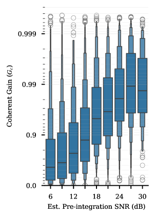
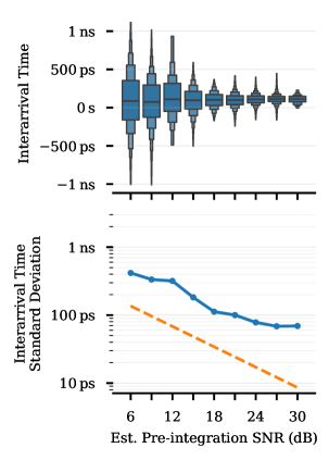
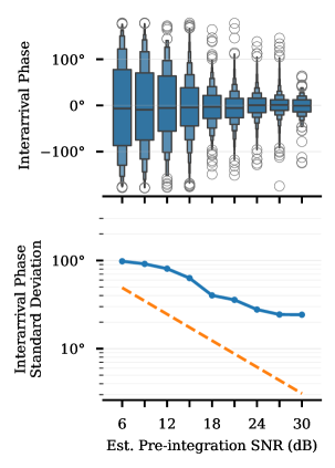
Figure 15: Electrical state coordination performance evaluation under varying average pre-integration snr of the received waveform measured at each node during the twtt process. The top row shows the absolute measured quantity, and the bottom row shows its standard deviation. In the interarrival time standard deviation, the outliers have been removed as discussed in Section V-C. The dashed line indicates the crlb.

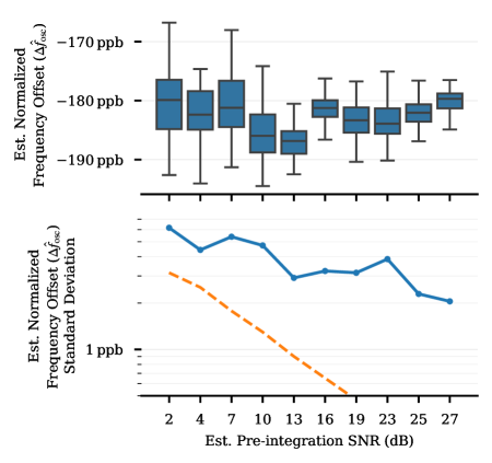
Figure 16: Estimated internode frequency offset and standard deviation under varying nominal pre-integration snr of the received waveform measured at each node during the twtt process. The top row shows the absolute measured quantity, and the bottom row shows its standard deviation, omitting outliers as discussed in Section V-C. The crlb, given by (25) using the nominal snr and average $\tau_{\mathrm{twtt}}=$55\text{\,}\mathrm{ms}$$, is indicated by the dashed line.

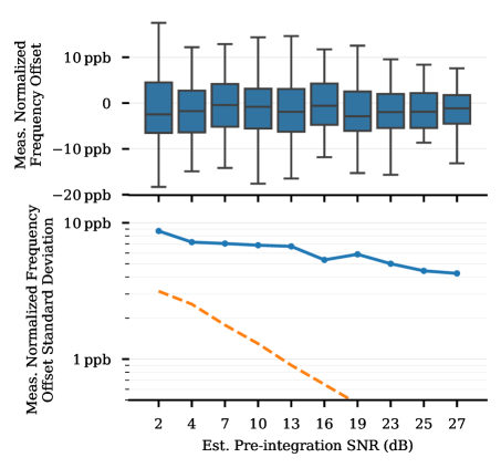
Figure 17: Measured internode “beamforming” frequency at oscilloscope under varying nominal pre-integration snr of the received ptt waveform at each node during the twtt process. The top row shows the absolute measured quantity, and the bottom row shows its standard deviation, omitting outliers as discussed in Section V-C. The crlb, given by (25) using the nominal snr and average $\tau_{\mathrm{twtt}}=$55\text{\,}\mathrm{ms}$$, is indicated by the dashed line.

In all experiments, standard deviation values are also plotted with the distributions of the measured data. Because the standard deviation is not a robust measure of statistical dispersion, outliers due to the host processor missing real-time processing deadlines causing synchronization retries are removed in the experiments with unbounded measurement values (interarrival time and internode frequency difference) prior to computing the standard deviation. Outliers are removed by iteratively removing data which exceeds $x$ standard deviations until all data fits within $x$ standard deviations; for the interarrival time dataset, $x=6$; for the smaller frequency difference dataset, $x=4$. Additionally, due to the significantly longer pulses used in frequency estimation, the host processing required to generate and transfer all the samples to the sdr increased appreciably, resulting in longer resynchronization intervals and decreasing overall coordination performance. Nonetheless, the frequency syntonization results still indicate good performance. Finally, statistics from each run are summarized in time domain plots and histograms, with markers indicating where outliers have been removed, in the appendices located in the supplemental materials.

V-D1 Signal-to-Noise Ratio

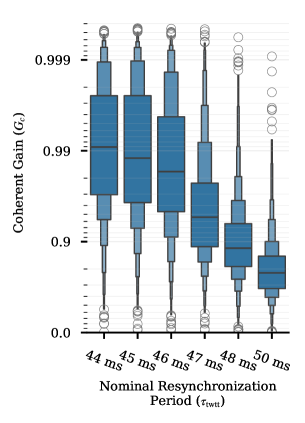
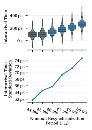
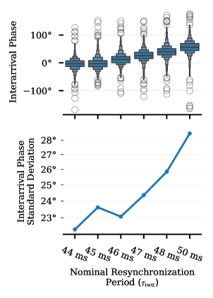
Figure 18: Electrical state coordination performance evaluation under varying resynchronization periods $\tau_{\mathrm{twtt}}$. The top row shows the absolute measured quantity; the bottom row shows the standard deviation. In the interarrival time standard deviation, the outliers have been removed as discussed in Section V-C. Across all measurements, an average Pre-integration snr of approximately $\mu=27$ dB and $\sigma=1$ was estimated.

In this experiment Configuration A was used to evaluate the coherent gain, interarrival time, and interarrival phase (Fig. 15), and estimated and measured internode beamforming frequency (Fig. 16 and Fig. 17) under varying average pre-integration snr (i.e., before filtering) for the twtt ptt waveform received at each node. As the average snr increases, the coordination performance improves, which can be seen in the median coherent gain which increases to a maximum where the snr reaches 27 dB, at which point a limit of about 0.99 is reached due to the static time and phase calibration values. The time difference of arrival has a relative constant median near $\sim$$100\text{\,}\mathrm{ps}$ due to unmatched static system delays, but the data spread decreases with snr, as expected approaching a timing standard deviation of $70\text{\,}\mathrm{ps}$. The interarrival phase maintained a zero-mean offset with a standard deviation of $\sim$$12.5\mathrm{°}$ at 30 dB snr.

The estimated and measured frequency syntonization performance plots are shown in Figs. 16 and 17, respectively. The absolute frequency offset estimates are shown on the top row of Fig. 16, which indicates a typical internode frequency offset of near $-182$ ppb and estimated frequency offset standard deviation of 2.04 ppb. The beamforming frequency offsets after compensation are shown in Fig. 17 which indicate a mean frequency error of $-1.25$ ppb across all snr with the standard deviation reaching $4.22$ ppb at a 33 dB snr. The crlb is also included using (25) as indicated by the dashed line. This crlb is computed using the nominal snr value and the average resynchronization period $\tau_{\mathrm{twtt}}=$55\text{\,}\mathrm{ms}$$.

V-D2 Resynchronization Period

This experiment used Configuration A to evaluate coordination performance under varying resynchronization period $\tau_{\mathrm{twtt}}$, shown in Fig. 18. The nominal resynchronization period was varied from $44\text{\,}\mathrm{ms}$—the minimum possible on the host due to software implementation and hardware limitations—to $50\text{\,}\mathrm{ms}$, at which the coherent gain performance begins to significantly decline due to the dominant system dynamics evolving faster than the resynchronization period.

V-D3 Two-Way Time Transfer Pulse Duration

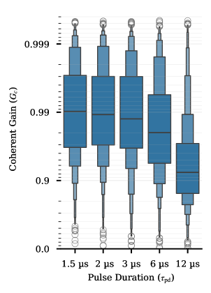
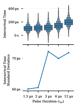
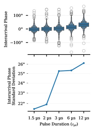
Figure 19: Electrical state coordination performance evaluation under varying twtt ptt durations $\tau_{\mathrm{pd}}$. The top row shows the absolute measured quantity, and the bottom row shows its standard deviation, omitting outliers as discussed in Section V-C. Across all measurements, an average pre-integration snr of approximately $\mu=27$ dB and $\sigma=1$ was estimated for $1.5\text{\,}\mathrm{\SIUnitSymbolMicro s}$–$3.0\text{\,}\mathrm{\SIUnitSymbolMicro s}$; however, due to an error, the snr estimator did not correctly estimate $1.5\text{\,}\mathrm{\SIUnitSymbolMicro s}$–$3.0\text{\,}\mathrm{\SIUnitSymbolMicro s}$, but similar snr are expected due to an identical system setup.

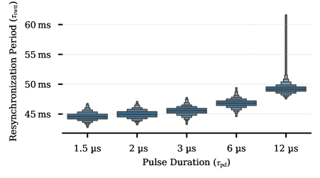
Figure 20: Resynchronization periods observed for various pulse durations. Results can be compared with those of Fig. 18 to determine expected performance due to resynchronization period at each pulse duration.

This experiment used Configuration A to evaluate coordination performance under varying twtt ptt durations $\tau_{\mathrm{pd}}$, shown in Fig. 19. In these experiments the interpulse spacing is held constant while $\tau_{\mathrm{pd}}$ is varied. According to (24), this should improve the time of arrival estimation; however, in practice, this increases the number of samples in the received pulse since the entire synchronization epoch is captured in a single receive frame on each sdr, which increases the number of samples required to process, increasing the computation latency, yielding decreasing performance as shown in Fig. 20. The long tail at $\tau_{\mathrm{pd}}=$ $12\text{\,}\mathrm{\SIUnitSymbolMicro s}$ is due to increased frequency of failure to meet real-time requirements due to the increased computational load of the matched filter. The interarrival delay and phase trends associated with the resynchronization period align with the varying resynchronization periods shown in Fig. 18, suggesting the degradation is due mostly to the processing latency increase—not the pulse duration itself—which is expected as the electrical states are not expected to be significantly varying over single or tens of microseconds.

V-D4 Synchronization Epoch Duration

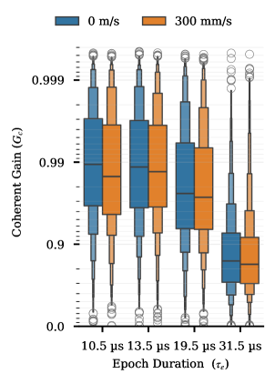
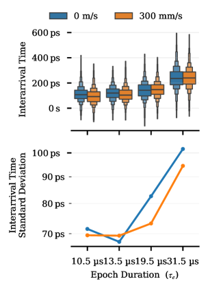
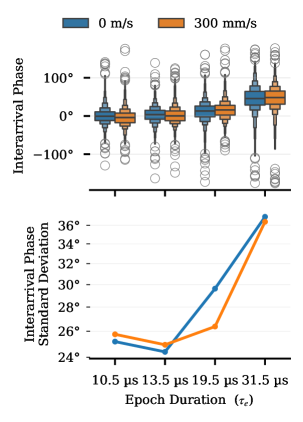
Figure 21: Electrical state coordination performance evaluation under varying twtt synchronization epoch durations $\tau_{e}$ under static and dynamic relative motion. The top row shows the absolute measured quantity, and the bottom row shows its standard deviation, omitting outliers as discussed in Section V-C. In the static measurements, an average pre-integration snr of approximately $\mu=27$ dB and $\sigma=1$ was estimated; in the dynamic measurements the average pre-integration snr were approximately $\mu=28.4$ dB and $\sigma=1.5$.

Figure 22: Resynchronization periods observed for various synchronization epoch durations under static and dynamic relative motion. Results can be compared with those of Fig. 18 to determine expected performance due to resynchronization period at each epoch duration.

This experiment used Configuration A to evaluate coordination performance over varying twtt synchronization epoch durations $\tau_{e}$ for both a static system and a system with relative internode motion, shown in Fig. 21. In these experiments, the antenna on node 0 was varied between 0 mm/s and 300 mm/s while the synchronization epoch duration was increased from $10.5\text{\,}\mathrm{\SIUnitSymbolMicro s}$ to $31.5\text{\,}\mathrm{\SIUnitSymbolMicro s}$. Similarly to the pulse duration experiments, due to the increased number of samples to process as the synchronization epoch duration increases, the latency increases, shown in Fig. 22; these again align with the performance degradations expected from the resynchronization shown in Fig. 18 and show little correlation with static versus moving platforms, again suggesting these degradations are due primarily to the increased latency due to the increased number of samples required to be processed via the matched filter per synchronization epoch.

V-D5 Node Scaling

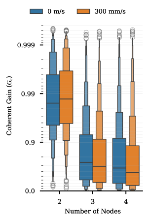
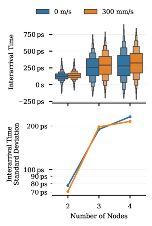
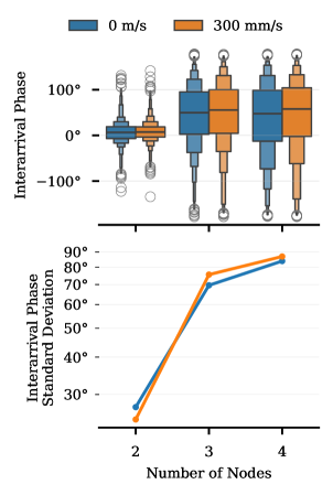
Figure 23: Electrical state coordination performance evaluation for various array sizes under static and dynamic relative motion. The top row shows the absolute measured quantity, and the bottom row shows its standard deviation, omitting outliers as discussed in Section V-C. Across all measurements, an average pre-integration snr of approximately $\mu=27$ dB and $\sigma=1$ was estimated for two and three nodes; in the four-node array, the average pre-integration snr were approximately $\mu=30$ dB and $\sigma=1$.

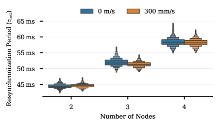
Figure 24: Resynchronization periods observed for various array sizes. Results can be compared with those of Fig. 18 to determine expected performance due to resynchronization period at each array size.

This experiment used Configuration A to evaluate the coordination performance for arrays of 2 to 4 nodes, shown in Fig. 23. Beamforming data was only collected from nodes $N_{0}$ and $N_{1}$; however, as nodes were added, their tdma slots were scheduled in between nodes $N_{0}$ and $N_{1}$ to illustrate the worst-case performance due to the longest synchronization epoch. As the number of nodes increases, the number of tdma time slots in the twtt also scales linearly, thus increasing the number of samples required to perform matched filtering on to compute the toa estimates for the twtt process, increasing latency and decreasing synchronization performance, as discussed previously. The resynchronization interval statistics for this experiment are summarized in Fig. 24. It is worth noting that even though the twtt could be conducted using space, frequency, or code orthogonality, instead of time orthogonality, the number of samples required to be matched filtered is constant in all cases.

V-D6 Reference Oscillator Frequency Offset

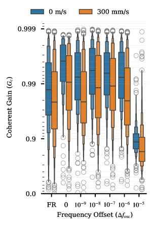
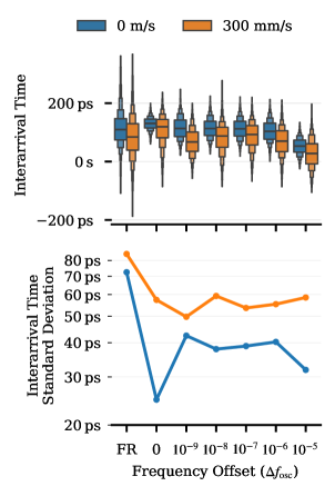
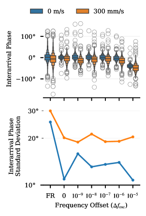
Figure 25: Electrical state coordination performance evaluation using known static frequency offsets generated using a signal generator, as described in Configuration B. The top row shows the absolute measured quantity, and the bottom row shows its standard deviation, omitting outliers as discussed in Section V-C. The data point labeled “FR” indicates both oscillators are “free-running,” i.e., not using an external frequency reference. Across all measurements, an average pre-integration snr of approximately $\mu=27$ dB and $\sigma=1$ was estimated.

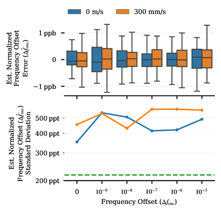
Figure 26: Estimated frequency offset between nodes (top) and its standard deviation (bottom) using Configuration B. The top row shows the absolute measured quantity, and the bottom row shows its standard deviation, omitting outliers as discussed in Section V-C. The crlb is indicated by the dashed line. Across all measurements the snr was estimated to have a mean value of 25.5 dB with a resynchronization interval of $\tau_{\mathrm{twtt}}=$55\text{\,}\mathrm{ms}$$ Note that “FR” is omitted as this plot represents estimator error and the true value of the frequency error between nodes is unknown.

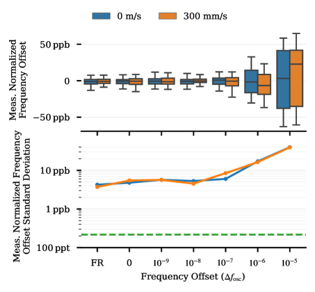
Figure 27: Internode beamforming frequency offsets measured at the oscilloscope in Configuration B. The top row shows the absolute measured quantity, and the bottom row shows its standard deviation, omitting outliers as discussed in Section V-C. The data point labeled “FR” indicates both oscillators are “free-running.”

This experiment used Configuration B to evaluate the accuracy of the system when estimating a known internode frequency offset $\Delta f_{\mathrm{osc}}^{(n,m)}$ by locking the system clocks together with a known static frequency offset generated by a signal generator. Known frequency offsets ranging from 0 to 10 ppm and free-running (FR) were evaluated under static and dynamic internode positions and the performance results are summarized in Figs. 25–27. There is a minimal change in coherent gain, time, and phase stability up to frequency offsets of 1 ppm with performance drop-off at 10 ppm due primarily to increased time and phase biases.

Figs. 26 and 27 show the estimated and measured frequency offsets, respectively, along with their standard deviations, omitting outliers due to the host processor not meeting real-time requirements as discussed in Section V-C, and crlb from (25) using the average snr across all measurements of 22.5 dB and average resynchronization period of $\tau_{\mathrm{twtt}}=$55\text{\,}\mathrm{ms}$$. The results for the estimated frequency error are shown in Fig. 26 which appears as zero-mean over all frequency offsets with minimal standard deviation. This trend is continued for the beamforming frequency errors measured at the oscilloscope, shown in Fig. 27, up to 1 ppm. After investigating the internode phase differences in the time domain (See experiments 26.6 and 26.13 Appendix J in the supplemental materials), the source of this error appears due to a harmonic sawtooth-like phase error which evolves on the order of microseconds, likely due to the pll designs, and thus cannot be compensated for using the resynchronization period on the order of milliseconds used in these experiments.

V-D7 Frequency Syntonization Method

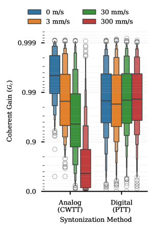
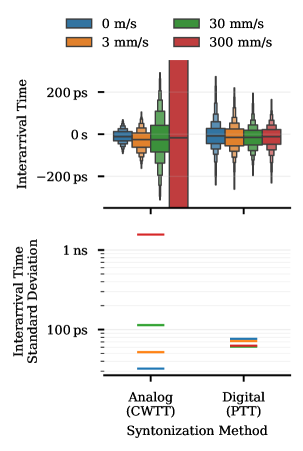
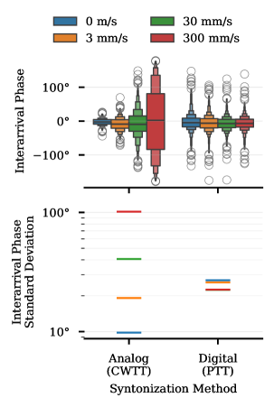
Figure 28: Electrical state coordination performance evaluation for the analog cwtt method versus the twtt-based fully-digital ptt approach described in this paper under varying relative motion. The top row shows the absolute measured quantity, and the bottom row shows its standard deviation, omitting outliers as discussed in Section V-C. The clipped data for $300\text{\,}\mathrm{m}\mathrm{m}\mathrm{/}\mathrm{s}$ interarrival time spans over approximately $\pm$$2.5\text{\,}\mathrm{ns}$, or $\pm$0.5 samples at $200\text{\,}\mathrm{M}\mathrm{S}\mathrm{a}\mathrm{/}\mathrm{s}$.

This experiment used Configuration C to evaluate the twtt-based fully-digital ptt time and frequency estimation technique described in this work relative to the analog cwtt-based syntonization technique used in prior works [36, 41, 42, 3]. In this technique the analog cwtt method is used for syntonization and the digital twtt method is used to compensate for the time-varying phase shift induced by the time-varying propagation delay of the cwtt clock signal received at the secondary nodes when the system is in motion. In this experiment, the linear guide was set to $0\text{\,}\mathrm{m}\mathrm{/}\mathrm{s}$, $3\text{\,}\mathrm{m}\mathrm{m}\mathrm{/}\mathrm{s}$, $30\text{\,}\mathrm{m}\mathrm{m}\mathrm{/}\mathrm{s}$, and $300\text{\,}\mathrm{m}\mathrm{m}\mathrm{/}\mathrm{s}$, with a range of movement of $0\text{\,}\mathrm{cm}$, $1\text{\,}\mathrm{cm}$, $10\text{\,}\mathrm{cm}$, and $100\text{\,}\mathrm{cm}$, respectively, centered about a distance of $\sim$$87\text{\,}\mathrm{cm}$ between nodes 0 and 1. While both systems perform satisfactorily in stationary scenarios, the analog cwtt frequency syntonization technique maintains the highest performance yielding nearly all measurements above $G_{c}>0.9$; in slowly moving scenarios of $3\text{\,}\mathrm{m}\mathrm{m}\mathrm{/}\mathrm{s}$, mimicking situations with slight oscillations in a static installment, performance is comparable between the two systems. However, in situations with more significant relative motion, the digital ptt twtt-based system performs significantly better. This is primarily due to the fact that phase of the received frequency reference varies rapidly due to the changing propagation delay and multipath in the environment; while the twtt process corrects for this periodically, even at modest speeds the received phase varies significantly faster than the rate of the twtt required to correct for unlocked oscillators resulting in lower performance overall. Furthermore, due to environmental multipath, this phase modulation on the received frequency reference waveform is difficult to predict due to platform motion alone, thus tracking this phase via kinematic models may also be challenging.

V-E Discussion

In these experiments the importance of the synchronization latency and resynchronization interval was shown to be one of the most significant parameters to maintaining a high level of coordination amongst nodes in the array. This highlights the need to minimize the latency required to compute the toa. There were several factors which contributed to the latency in the demonstrated setup which can be improved by

1. minimizing the data transfer before toa computation, i.e., process the data close to the digitizer,

2. increasing the rate of computation by using efficient streaming data processor architectures (such as fpga or gpu), and

3. reducing the computational complexity of the toa estimation algorithm.

In this work, approximately half of the cycle time latency was due to the latency induced by the transport between the sdr and host, as well as overhead due to serialization and deserialization used in ipc, while the remaining half was computational load. Both concerns may be addressed by moving the signal processing closer to the data converters, which eliminates the Ethernet transport latency and ipc overhead, and can improve bandwidth by utilizing the on-device fpga to perform efficient stream processing which is not well suited to the general-purpose processor found on the host computer.

An alternate approach to improving the coordination performance was shown in Section V-D7, comparing the fully-digital method to the analog cwtt-based approach, that, for static or nearly static scenarios, the analog approach can obtain high levels of coordination while requiring significantly lower resynchronization intervals, minimizing the software complexity, and overall computational requirements of the system. In static systems where a continuous frequency reference is amenable, the cwtt approach may be a simpler solution to achieve high levels of coordination accuracy.

Finally, while many prior works have been referenced demonstrating time, phase, and frequency coordination in open-loop wirelessly coordinated cda, due to varying performance measurement techniques and reporting of coordination parameters used, a direct comparison between works is challenging. However, with respect to frequency syntonization performance, we achieve results within a similar order of magnitude to current similar state-of-the art works presented in [44] and [47] on the order of single parts per billion.

VI Conclusion

In this work we present a novel, fully-digital high-accuracy twtt-based joint time and frequency coordination system for cda using unmodified cots hardware and without relying on external time or frequency references such as gnss; we demonstrate that the fully-digital approach shows no significant difference in performance in a system with moderate relative internode velocity; and we demonstrate an internode beamforming frequency rmse as low as 3.73 ppb in a dynamic case with time and phase deviations as low as $60\text{\,}\mathrm{ps}$ and demonstrate median coherent gains above 99 % with optimized coordination parameters. This demonstrates a significant step towards fully wireless mobile cda capable of coherent transmit and receive beamforming for the next generation of mobile wireless communication and sensing systems.

References

- [1] S. Prager, M. S. Haynes, and M. Moghaddam, “Wireless subnanosecond rf synchronization for distributed ultrawideband software-defined radar networks,” IEEE Transactions on Microwave Theory and Techniques, vol. 68, no. 11, pp. 4787–4804, 2020.
- [2] A. Schlegel, J. M. Merlo, and J. A. Nanzer, “Coherent distributed bistatic radar using wireless frequency syntonization and internode ranging,” IEEE Microwave and Wireless Technology Letters, vol. 33, no. 9, pp. 1393–1396, 2023.
- [3] J. M. Merlo, S. Wagner, J. Lancaster, and J. A. Nanzer, “Fully wireless coherent distributed phased array system for networked radar applications,” IEEE Microwave and Wireless Technology Letters, vol. 34, no. 6, pp. 837–840, 2024.
- [4] J. Aguilar, D. Werbunat, V. Janoudi, C. Bonfert, and C. Waldschmidt, “Uncoupled digital radars creating a coherent sensor network,” IEEE Journal of Microwaves, vol. 4, no. 3, pp. 459–472, 2024.
- [5] J. M. Merlo and J. A. Nanzer, “Distributed interferometric radar for radial and angular velocity measurement,” in 2024 IEEE International Symposium on Antennas and Propagation and INCUSNC-URSI Radio Science Meeting (AP-SINC-USNC-URSI), 2024, pp. 1127–1128.
- [6] R. H. Kenney, J. G. Metcalf, and J. W. McDaniel, “Wireless distributed frequency and phase synchronization for mobile platforms in cooperative digital radar networks,” IEEE Transactions on Radar Systems, vol. 2, pp. 268–287, 2024.
- [7] ——, “Concept and theoretical performance analysis for decentralised digital synchronisation in distributed radar sensor networks,” IET Radar, Sonar & Navigation, vol. 19, no. 1, p. e12687, 2025.
- [8] T. Nusrat and S. Vakalis, “Addressing specularity: Millimeter-wave radar with distributed repeater apertures,” IEEE Transactions on Microwave Theory and Techniques, pp. 1–10, 2024.
- [9] D. Werbunat, J. Aguilar, M. Almarashly, V. Janoudi, S. Stephany, D. G. Gaviria, A. Ç. Ulusoy, and C. Waldschmidt, “On the synchronization of uncoupled multistatic PMCW radars,” IEEE Transactions on Microwave Theory and Techniques, vol. 72, no. 8, pp. 4932–4944, 2024.
- [10] S. Shen, X. Niu, J. Guo, Z. Zhang, and S. Han, “High-resolution collaborative forward-looking imaging using distributed MIMO arrays,” Remote Sensing, vol. 16, no. 21, 2024.
- [11] D. Tagliaferri, M. Rizzi, S. Tebaldini, M. Nicoli, I. Russo, C. Mazzucco, A. V. Monti-Guarnieri, C. M. Prati, and U. Spagnolini, “Cooperative synthetic aperture radar in an urban connected car scenario,” in 2021 1st IEEE International Online Symposium on Joint Communications & Sensing (JC&S). IEEE, 2021, pp. 1–4.
- [12] V. Janoudi, P. Schoeder, T. Grebner, N. Appenrodt, J. Dickmann, and C. Waldschmidt, “Signal model for coherent processing of uncoupled and low frequency coupled MIMO radar networks,” IEEE Journal of Microwaves, vol. 4, no. 1, pp. 69–85, 2024.
- [13] D. Werbunat, B. Woischneck, J. Lerch, B. Schweizer, R. Michev, C. Bonfert, J. Hasch, and C. Waldschmidt, “Multichannel repeater for coherent radar networks enabling high-resolution radar imaging,” IEEE Transactions on Microwave Theory and Techniques, vol. 72, no. 5, pp. 3247–3259, 2024.
- [14] P. Fenske, T. Koegel, R. Ghasemi, D. Gunders-Hunt, and M. Vossiek, “Integrated self-contained trajectory estimation and multistatic SAR imaging in a non-static uncoupled bistatic radar network,” IEEE Journal of Microwaves, vol. 5, no. 3, pp. 600–615, 2025.
- [15] K. W. Choi, A. A. Aziz, D. Setiawan, N. M. Tran, L. Ginting, and D. I. Kim, “Distributed wireless power transfer system for internet of things devices,” IEEE Internet of Things Journal, vol. 5, no. 4, pp. 2657–2671, 2018.
- [16] J. Brunet, A. Ayling, and A. Hajimiri, “Transmitarrays for wireless power transfer on Earth and in space,” IEEE Journal of Microwaves, pp. 1–12, 2024.
- [17] I. Mahbub, A. B. Patwary, R. Mahin, and S. Roy, “Far-field wireless power beaming to mobile receivers using distributed, coherent phased arrays: A review of the critical components of a distributed wireless power beaming system,” IEEE Microwave Magazine, vol. 25, no. 5, pp. 72–94, 2024.
- [18] S. M. Ellison, J. M. Merlo, and J. A. Nanzer, “Distributed antenna array dynamics for secure wireless communication,” IEEE Transactions on Antennas and Propagation, vol. 70, no. 4, pp. 2740–2749, 2022.
- [19] J. Holtom, O. Ma, A. Herschfelt, I. Lenz, Y. Li, and D. W. Bliss, “Distributed coherent mesh beamforming (DisCoBeaM) for robust wireless communications,” IEEE Transactions on Wireless Communications, vol. 23, no. 11, pp. 15 814–15 828, 2024.
- [20] K. S. Bondada, D. J. Jakubisin, K. Said, R. M. Buehrer, and L. Liu, “Wireless mobile distributed-mimo for 6g,” in 2024 IEEE 100th Vehicular Technology Conference (VTC2024-Fall), 2024, pp. 1–7.
- [21] Z. Xu, G. Chen, R. Fernandez, Y. Gao, and R. Tafazolli, “Enhancement of direct LEO satellite-to-smartphone communications by distributed beamforming,” IEEE Transactions on Vehicular Technology, pp. 1–13, 2024.
- [22] G. Sun, J. Li, A. Wang, Q. Wu, Z. Sun, and Y. Liu, “Secure and energy-efficient UAV relay communications exploiting collaborative beamforming,” IEEE Transactions on Communications, vol. 70, no. 8, pp. 5401–5416, 2022.
- [23] M. B. Quadrelli, R. Hodges, V. Vilnrotter, S. Bandyopadhyay, F. Tassi, and S. Bevilacqua, “Distributed swarm antenna arrays for deep space applications,” in 2019 IEEE Aerospace Conference, 2019, pp. 1–15.
- [24] “2020 NASA technology taxonomy,” National Aeronautics and Space Administration, Tech. Rep. HQ-E-DAA-TN76545, Jan. 2020.
- [25] J. A. Nanzer, S. R. Mghabghab, S. M. Ellison, and A. Schlegel, “Distributed phased arrays: Challenges and recent advances,” IEEE Transactions on Microwave Theory and Techniques, vol. 69, no. 11, pp. 4893–4907, 2021.
- [26] D. Brown, G. Prince, and J. McNeill, “A method for carrier frequency and phase synchronization of two autonomous cooperative transmitters,” in IEEE 6th Workshop on Signal Processing Advances in Wireless Communications, 2005., 2005, pp. 260–264.
- [27] M. Seo, M. Rodwell, and U. Madhow, “A feedback-based distributed phased array technique and its application to 60-GHz wireless sensor network,” in 2008 IEEE MTT-S International Microwave Symposium Digest, 2008, pp. 683–686.
- [28] D. R. Brown III and H. V. Poor, “Time-slotted round-trip carrier synchronization for distributed beamforming,” IEEE Transactions on Signal Processing, vol. 56, no. 11, pp. 5630–5643, 2008.
- [29] R. Mudumbai, D. R. B. Iii, U. Madhow, and H. V. Poor, “Distributed transmit beamforming: challenges and recent progress,” IEEE Communications Magazine, vol. 47, no. 2, pp. 102–110, 2009.
- [30] R. D. Preuss and D. R. Brown, III, “Two-way synchronization for coordinated multicell retrodirective downlink beamforming,” IEEE Transactions on Signal Processing, vol. 59, no. 11, pp. 5415–5427, 2011.
- [31] P. Bidigare, M. Oyarzyn, D. Raeman, D. Chang, D. Cousins, R. O’Donnell, C. Obranovich, and D. R. Brown, “Implementation and demonstration of receiver-coordinated distributed transmit beamforming across an ad-hoc radio network,” in 2012 Conference Record of the Forty Sixth Asilomar Conference on Signals, Systems and Computers (ASILOMAR), 2012, pp. 222–226.
- [32] F. Quitin, M. M. U. Rahman, R. Mudumbai, and U. Madhow, “A scalable architecture for distributed transmit beamforming with commodity radios: Design and proof of concept,” IEEE Transactions on Wireless Communications, vol. 12, no. 3, pp. 1418–1428, 2013.
- [33] F. Quitin, A. T. Irish, and U. Madhow, “A scalable architecture for distributed receive beamforming: Analysis and experimental demonstration,” IEEE Transactions on Wireless Communications, vol. 15, no. 3, pp. 2039–2053, 2016.
- [34] S. Hanna and D. Cabric, “Distributed transmit beamforming: Design and demonstration from the lab to UAVs,” IEEE Transactions on Wireless Communications, vol. 22, no. 2, pp. 778–792, 2023.
- [35] J. A. Nanzer, R. L. Schmid, T. M. Comberiate, and J. E. Hodkin, “Open-loop coherent distributed arrays,” IEEE Transactions on Microwave Theory and Techniques, vol. 65, no. 5, pp. 1662–1672, 2017.
- [36] O. Abari, H. Rahul, D. Katabi, and M. Pant, “Airshare: Distributed coherent transmission made seamless,” in 2015 IEEE Conference on Computer Communications (INFOCOM), 2015, pp. 1742–1750.
- [37] H. Yan, S. Hanna, K. Balke, R. Gupta, and D. Cabric, “Software defined radio implementation of carrier and timing synchronization for distributed arrays,” in 2019 IEEE Aerospace Conference, 2019, pp. 1–12.
- [38] H. Ouassal, T. Rocco, M. Yan, and J. A. Nanzer, “Decentralized frequency synchronization in distributed antenna arrays with quantized frequency states and directed communications,” IEEE Trans. Antennas Propag., vol. 68, no. 7, pp. 5280–5288, 2020.
- [39] K. Alemdar, D. Varshney, S. Mohanti, U. Muncuk, and K. Chowdhury, “RFClock: timing, phase and frequency synchronization for distributed wireless networks,” in Proceedings of the 27th Annual International Conference on Mobile Computing and Networking, 2021, pp. 15–27.
- [40] H. Ouassal, M. Yan, and J. A. Nanzer, “Decentralized frequency alignment for collaborative beamforming in distributed phased arrays,” IEEE Trans. Wireless Commun., vol. 20, no. 10, pp. 6269–6281, 2021.
- [41] S. R. Mghabghab and J. A. Nanzer, “Open-loop distributed beamforming using wireless frequency synchronization,” IEEE Transactions on Microwave Theory and Techniques, vol. 69, no. 1, pp. 896–905, 2021.
- [42] J. M. Merlo, S. R. Mghabghab, and J. A. Nanzer, “Wireless picosecond time synchronization for distributed antenna arrays,” IEEE Transactions on Microwave Theory and Techniques, vol. 71, no. 4, pp. 1720–1731, 2023.
- [43] S. Hanna, E. Krijestorac, and D. Cabric, “Destination-feedback free distributed transmit beamforming using guided directionality,” IEEE Transactions on Mobile Computing, vol. 22, no. 10, pp. 5858–5869, 2023.
- [44] R. H. Kenney and J. W. McDaniel, “All-digital carrier frequency synchronization for distributed radar sensor networks,” in 2024 IEEE/MTT-S International Microwave Symposium - IMS 2024, 2024, pp. 493–496.
- [45] N. Shandi, J. M. Merlo, and J. A. Nanzer, “Decentralized picosecond synchronization for distributed wireless systems,” IEEE Transactions on Communications, 2024.
- [46] J. M. Merlo, N. Shandi, M. Dula, A. Bhattacharyya, and J. A. Nanzer, “Fully wireless collaborative beamforming using a three-element coherent distributed phased array,” in 2024 IEEE International Symposium on Phased Array Systems & Technology (PAST), Boston, Massachusetts, USA, Oct. 2024.
- [47] R. Ghasemi, T. Koegel, P. Fenske, R. Schober, and M. Vossiek, “Time and frequency synchronization for real-time wireless digital communication systems,” in 2024 15th German Microwave Conference (GeMiC), 2024, pp. 13–16.
- [48] M. M. Rahman, S. Dasgupta, and R. Mudumbai, “A distributed consensus approach to synchronization of rf signals,” in 2012 IEEE Statistical Signal Processing Workshop (SSP), 2012, pp. 281–284.
- [49] M. Rashid and J. A. Nanzer, “Frequency and phase synchronization in distributed antenna arrays based on consensus averaging and kalman filtering,” IEEE Transactions on Wireless Communications, vol. 22, no. 4, pp. 2789–2803, 2023.
- [50] ——, “High accuracy distributed kalman filtering for synchronizing frequency and phase in distributed phased arrays,” IEEE Signal Processing Letters, vol. 30, pp. 688–692, 2023.
- [51] ——, “Online expectation-maximization based frequency and phase consensus in distributed phased arrays,” IEEE Transactions on Communications, vol. 71, no. 6, pp. 3721–3735, 2023.
- [52] J. Levine, “A review of time and frequency transfer methods,” Metrologia, vol. 45, no. 6, p. S162, 2008.
- [53] D. Hanson, “Fundamentals of two-way time transfers by satellite,” in Proceedings of the 43rd Annual Symposium on Frequency Control, 1989, pp. 174–178.
- [54] D. Kirchner, “Two-way time transfer via communication satellites,” Proceedings of the IEEE, vol. 79, no. 7, pp. 983–990, 1991.
- [55] “IEEE standard for a precision clock synchronization protocol for networked measurement and control systems,” IEEE Std 1588-2019 (Revision ofIEEE Std 1588-2008), pp. 1–499, 2020.
- [56] J. Serrano, M. Lipinski, T. Wlostowski, E. Gousiou, E. van der Bij, M. Cattin, and G. Daniluk, “The white rabbit project,” 2013.
- [57] R. K. Pooler, J. S. Sunderlin, R. H. Tillman, and R. L. Schmid, “A precise RF time transfer method for coherent distributed system applications,” in 2018 USNC-URSI Radio Science Meeting (Joint with AP-S Symposium). IEEE, 2018, pp. 5–6.
- [58] S. R. Mghabghab, A. Schlegel, and J. A. Nanzer, “Adaptive distributed transceiver synchronization over a 90 m microwave wireless link,” IEEE Transactions on Antennas and Propagation, vol. 70, no. 5, pp. 3688–3699, 2022.
- [59] C. Chen and A. Babakhani, “Wireless synchronization and spatial combining of widely spaced mm-wave arrays in 65-nm cmos,” IEEE Transactions on Microwave Theory and Techniques, vol. 65, no. 11, pp. 4418–4427, 2017.
- [60] A. Kiyaei, W. Ahmad, S. Zakir, E. M. A. Seragi, A. H. Shah, and S. Zeinolabedinzadeh, “Interference-tolerant wireless distributed beamforming receiver array with low-latency frequency synchronization,” IEEE Transactions on Microwave Theory and Techniques, pp. 1–14, 2024.
- [61] D. Allan, “Time and frequency (time-domain) characterization, estimation, and prediction of precision clocks and oscillators,” IEEE Transactions on Ultrasonics, Ferroelectrics, and Frequency Control, vol. 34, no. 6, pp. 647–654, 1987.
- [62] D. W. Allan, J. Barnes, F. Cordara, M. Garvey, W. Hanson, R. Kinsman, J. Kusters, R. Smythe, and F. L. Walls, “Precision oscillators: dependence of frequency on temperature, humidity and pressure,” in Proceedings of the 1992 IEEE Frequency Control Symposium, 1992, pp. 782–793.
- [63] H. Hellwig, “Environmental sensitivities of precision frequency sources,” IEEE Transactions on Instrumentation and Measurement, vol. 39, no. 2, pp. 301–306, 1990.
- [64] R. Filler, “The acceleration sensitivity of quartz crystal oscillators: a review,” IEEE Transactions on Ultrasonics, Ferroelectrics, and Frequency Control, vol. 35, no. 3, pp. 297–305, 1988.
- [65] J. Kosinski, “Theory and design of crystal oscillators immune to acceleration: present state of the art,” in Proceedings of the 2000 IEEE/EIA International Frequency Control Symposium and Exhibition (Cat. No.00CH37052), 2000, pp. 260–268.
- [66] F. Walls and J. Vig, “Fundamental limits on the frequency stabilities of crystal oscillators,” IEEE Transactions on Ultrasonics, Ferroelectrics, and Frequency Control, vol. 42, no. 4, pp. 576–589, 1995.
- [67] J. Vanier, J. Gagnepain, W. Riley, F. Walls, and M. Granveaud, “Aging, warm-up time and retrace: important characteristics of standard frequency generators (proposal for IEEE standards project P1193),” in Proceedings of the 1992 IEEE Frequency Control Symposium, 1992, pp. 807–815.
- [68] H. Zhou, C. Nicholls, T. Kunz, and H. Schwartz, “Frequency accuracy & stability dependencies of crystal oscillators,” Carleton University, Systems and Computer Engineering, Technical Report SCE-08-12, 2008.
- [69] J. A. Barnes, A. R. Chi, L. S. Cutler, D. J. Healey, D. B. Leeson, T. E. McGunigal, J. A. Mullen, W. L. Smith, R. L. Sydnor, R. F. C. Vessot, and G. M. R. Winkler, “Characterization of frequency stability,” IEEE Transactions on Instrumentation and Measurement, vol. IM-20, no. 2, pp. 105–120, 1971.
- [70] M. Mossammaparast, P. Mullin, L. Ronchetti, R. Koehler, and N. Tiches, “Techniques on crystal oscillator vibration compensation,” Journal of Physics: Conference Series, vol. 2889, no. 1, p. 012010, nov 2024.
- [71] G. Klimovitch, “A nonlinear theory of near-carrier phase noise in free-running oscillators,” in Proceedings of the 2000 Third IEEE International Caracas Conference on Devices, Circuits and Systems (Cat. No.00TH8474), 2000, pp. T80/1–T80/6.
- [72] A. Chorti and M. Brookes, “A spectral model for rf oscillators with power-law phase noise,” IEEE Transactions on Circuits and Systems I: Regular Papers, vol. 53, no. 9, pp. 1989–1999, 2006.
- [73] D. A. Howe, Frequency Stability. John Wiley & Sons, Ltd, 2005.
- [74] F. Gardner, Phaselock Techniques, 3rd ed. Wiley, 2005.
- [75] V. Manassewitsch, Frequency Synthesizers: Theory and Design, 3rd ed. Wiley, 1990.
- [76] S. R. Kurtz, “Mixers as phase detectors,” Watkins-Johnson Company, Tech. Rep. Vol. 5 No. 1, January/February 1978.
- [77] J. M. Merlo and J. A. Nanzer, “Picosecond non-line-of-sight wireless time and frequency synchronization for coherent distributed aperture antenna arrays,” in International Union of Radio Scientists General Assembly, August 2023.
- [78] H. Van Trees, Detection, Estimation, and Modulation Theory, Part III: Radar-Sonar Signal Processing and Gaussian Signals in Noise, ser. Detection, Estimation, and Modulation Theory. Wiley, 2001, vol. 3.
- [79] J. A. Nanzer, M. D. Sharp, and D. Richard Brown, “Bandpass signal design for passive time delay estimation,” in 2016 50th Asilomar Conference on Signals, Systems and Computers, 2016, pp. 1086–1091.
- [80] J. A. Nanzer and M. D. Sharp, “On the estimation of angle rate in radar,” IEEE Trans. Antennas Propag., vol. 65, no. 3, pp. 1339–1348, 2017.
- [81] M. Richards, Fundamentals of Radar Signal Processing, Second Edition. McGraw-Hill Education, 2014.
- [82] S. M. Ellison, “High accuracy wireless ranging for phase alignment in distributed microwave beamforming arrays,” Ph.D. dissertation, Michigan State University, 2020.
- [83] R. Moddemeijer, “On the determination of the position of extrema of sampled correlators,” IEEE Trans. Signal Process., vol. 39, no. 1, pp. 216–219, 1991.
- [84] S. R. Mghabghab and J. A. Nanzer, “Microwave ranging via least-squares estimation of spectrally sparse signals in software-defined radio,” IEEE Microw. Wireless Compon. Lett., vol. 32, no. 2, pp. 161–164, 2022.
- [85] P. Chatterjee and J. A. Nanzer, “A study of coherent gain degradation due to node vibrations in open loop coherent distributed arrays,” in 2017 USNC-URSI Radio Science Meeting (Joint with AP-S Symposium), 2017, pp. 115–116.
- [86] S. R. Mghabghab and J. A. Nanzer, “Impact of VCO and PLL phase noise on distributed beamforming arrays with periodic synchronization,” IEEE Access, vol. 9, pp. 56 578–56 588, 2021.
- [87] C. E. Duchon, “Lanczos filtering in one and two dimensions,” Journal of Applied Meteorology and Climatology, vol. 18, no. 8, pp. 1016 – 1022, 1979.
- [88] F. J. Harris, Multirate Signal Processing For Communication Systems, 2nd ed. Pearson Education, 2021.
- [89] C. R. Harris, K. J. Millman, S. J. van der Walt, R. Gommers, P. Virtanen, D. Cournapeau, E. Wieser, J. Taylor, S. Berg, N. J. Smith, R. Kern, M. Picus, S. Hoyer, M. H. van Kerkwijk, M. Brett, A. Haldane, J. F. del Río, M. Wiebe, P. Peterson, P. Gérard-Marchant, K. Sheppard, T. Reddy, W. Weckesser, H. Abbasi, C. Gohlke, and T. E. Oliphant, “Array programming with NumPy,” Nature, vol. 585, no. 7825, pp. 357–362, Sep. 2020.
- [90] S. K. Lam, A. Pitrou, and S. Seibert, “Numba: a LLVM-based python JIT compiler,” in Proceedings of the Second Workshop on the LLVM Compiler Infrastructure in HPC, ser. LLVM ’15. New York, NY, USA: Association for Computing Machinery, 2015.
- [91] S. Kay, “A fast and accurate single frequency estimator,” IEEE Transactions on Acoustics, Speech, and Signal Processing, vol. 37, no. 12, pp. 1987–1990, 1989.
- [92] H. Hofmann, H. Wickham, and K. Kafadar, “Letter-value plots: Boxplots for large data,” Journal of Computational and Graphical Statistics, vol. 26, no. 3, pp. 469–477, 2017.