GGBall: Graph Generative Model on Poincaré Ball

Abstract

Generating graphs with hierarchical structures remains a fundamental challenge due to the limitations of Euclidean geometry in capturing exponential complexity. Here we introduce GGBall, a novel hyperbolic framework for graph generation that integrates geometric inductive biases with modern generative paradigms. GGBall combines a Hyperbolic Vector-Quantized Autoencoder (HVQVAE) with a Riemannian flow matching prior defined via closed-form geodesics. This design enables flow-based priors to model complex latent distributions, while vector quantization helps preserve the curvature-aware structure of the hyperbolic space. We further develop a suite of hyperbolic GNN and Transformer layers that operate entirely within the manifold, ensuring stability and scalability. Empirically, our model reduces degree MMD by over 75% on Community-Small and over 40% on Ego-Small compared to state-of-the-art baselines, demonstrating an improved ability to preserve topological hierarchies. These results highlight the potential of hyperbolic geometry as a powerful foundation for the generative modeling of complex, structured, and hierarchical data domains. Our code is available at here.

1 Introduction

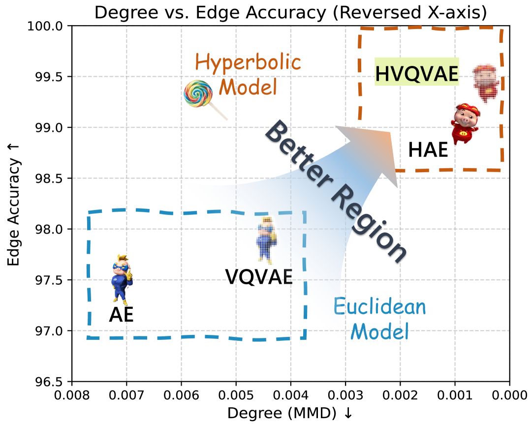
Figure 1: Degree distribution similarity and edge reconstruction accuracy on reconstructed dataset. Hyperbolic models consistently outperform Euclidean baselines.

Graph generation plays a central role in many scientific and engineering domains, including molecular design, material discovery, and social network modeling (Miller et al., 2025; Shi et al., 2020; Reiser et al., 2022; Luo et al., 2021; Wang et al., 2021). Recent advances in deep generative models have enabled powerful data-driven approaches to this task. Most existing models operate directly in the discrete graph space, where generation proceeds by sequentially constructing or refining nodes and edges. For instance, diffusion-based models such as GDSS (Jo et al., 2022) and DiGress (Vignac et al., 2023) iteratively denoise graphs in a discrete space, while autoregressive models like GraphRNN (You et al., 2018) and GRAN (Liao et al., 2019) build graphs one node or edge at a time, modeling structural dependencies step-by-step. These approaches offer fine-grained control and explicitly model structural dependencies in the discrete graph domain.

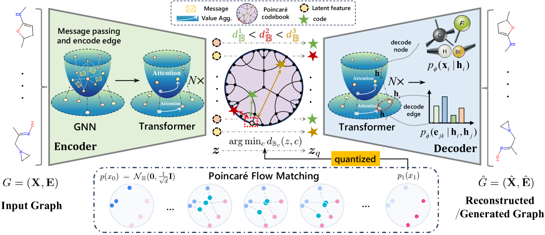
Figure 2: Overview of our hyperbolic graph generation framework. We encode graphs into a hyperbolic latent space using a Poincaré GNN and geodesic-attention Transformer. The latent representations are quantized via a Poincaré codebook and modeled with a Poincaré flow prior. A hyperbolic Transformer then decodes the latent code to reconstruct or generate graphs, enabling structure-aware generation in non-Euclidean geometry.

While these models have shown promise, graph generation remains challenging due to the discrete, combinatorial, and often hierarchical nature of graph data (Guo and Zhao, 2022). To address these issues, latent space generation has emerged as a scalable and flexible alternative. By encoding graphs into continuous latent representations and decoding from this space, methods like GraphVAE (Simonovsky and Komodakis, 2018) and VQGAE (Boget et al., 2023) enable efficient one-shot generation. Nevertheless, these models typically rely on Euclidean latent spaces, which are ill-suited for capturing the hierarchical and compositional nature of real-world graphs, such as community structures and power-law degree distributions (Krioukov et al., 2010).

This geometric mismatch motivates our shift to hyperbolic space, a natural framework for hierarchical representation learning (Mathieu et al., 2019). Unlike Euclidean embeddings that distort parent-child relationships, hyperbolic geometry intrinsically preserves graph hierarchies through its exponentially expanding volume (Krioukov et al., 2010; Chami et al., 2019; Ganea et al., 2018; Sarkar, 2011). As demonstrated in Figure 1, hyperbolic latent models (e.g., HAE, HVQVAE) achieve superior alignment with power-law degree distributions (4$\times$ lower MMD) and higher edge reconstruction accuracy compared to Euclidean counterparts on Community dataset.

Building on these insights, we present GGBall, the first Graph Generation framework built upon the Poincaré Ball model of hyperbolic space. Unlike existing approaches that operate in Euclidean or discrete graph space, GGBall encodes graphs into discrete, curvature-aware latent variables and performs generation directly in hyperbolic space. Specifically, we convert a standard Euclidean latent generative pipeline (Rombach et al., 2022) into a fully hyperbolic one: For the encoder, we design a Hyperbolic Vector-Quantized Autoencoder (HVQVAE) that captures graph structure via discrete tokens in the Poincaré ball, initialized through geodesic clustering and optimized using Riemannian methods. For the latent generative process, we leverage flow matching in hyperbolic space to model expressive priors without relying on predefined noise distributions. For architectural support, we develop a modular suite of hyperbolic GNN and Transformer layers that operate entirely within the manifold, ensuring numerical stability and scalability.

Our method achieves state-of-the-art performance on synthetic graphs with hierarchical structure. On Community-Small and Ego-Small, GGBall reduces degree distributional discrepancies by over 75% compared to Euclidean state-of-the-art baselines, and surpasses recent graph-space diffusion and flow models on Community-Small. These improvements highlight the strength of hyperbolic latent geometry in modeling modular, tree-like structures. On molecular graphs (QM9), GGBall also delivers strong results, achieving 98.50% novelty and 86.42% validity, demonstrating its ability to generate diverse and chemically plausible molecules.

2 Preliminaries and Problem Definition

To support our hyperbolic generative framework, we briefly review the Poincaré ball model as the underlying latent space in Section 2.1, followed by the formulation of graph generation in non-Euclidean geometry in Section 2.2.

2.1 Hyperbolic Geometry

2.1.1 Riemannian Manifold

A Riemannian manifold $(\mathcal{M},\mathfrak{g})$ is a smooth manifold equipped with a Riemannian metric tensor field $\mathfrak{g}$, which smoothly assigns to each point $x\in\mathcal{M}$ an inner product $\mathfrak{g}_{x}:\mathcal{T}_{x}\mathcal{M}\times\mathcal{T}_{x}\mathcal{M}\rightarrow\mathbb{R}$ on its tangent space $\mathcal{T}_{x}\mathcal{M}$ (Gallot et al., 1990). For a $n$-dimensional manifold, each tangent space $\mathcal{T}_{x}\mathcal{M}$ is locally isomorphic to $\mathbb{R}^{n}$, providing a linear approximation of the manifold at $x$.

2.1.2 Hyperbolic Space and Poincaré Ball Model

Hyperbolic space is a Riemannian manifold of constant negative curvature $-c$, offering a geometric framework for hierarchical data representation. Among its isomorphic models, the Poincaré ball model $(\mathbb{B}_{c}^{n},\mathfrak{g}_{c})$ is widely adopted in machine learning due to its conformal structure and numerical stability. Here, $\mathbb{B}_{c}^{n}=\{\bm{x}\in\mathbb{R}^{n}\;|\;c\|\bm{x}\|^{2}<1\}$ defines an open ball of radius $1/\sqrt{c}$, and the metric tensor $\mathfrak{g}_{c}^{x}=(\lambda_{c}^{x})^{2}\mathbf{I}_{n}$ scales Euclidean distances by the conformal factor $\lambda_{c}^{x}=2(1-c\|\bm{x}\|^{2})^{-1}$. This induces a Riemannian inner product $\langle\bm{u},\bm{v}\rangle_{c}^{x}=(\lambda_{c}^{x})^{2}\langle\bm{u},\bm{v}\rangle$ for $\bm{u},\bm{v}\in\mathcal{T}_{x}\mathbb{B}_{c}^{n}$ (Ungar, 2008). To enable algebraic operations on hyperbolic coordinates, the Möbius gyrovector framework extends vector space axioms to gyrovectors. The basic binary operation is denoted as the Möbius addition $\oplus_{c}:\mathbb{B}_{c}^{n}\times\mathbb{B}_{c}^{n}\rightarrow\mathbb{B}_{c}^{n}$, which is a noncommutaive and nonassociative addition. We provide a detailed introduction of basic operations in Appendix D.4 and D.5.

2.1.3 Graphs in Hyperbolic Space

Hyperbolic space is well-suited for embedding graphs with hierarchical or tree-like structures, thanks to its exponential volume growth and negative curvature. Prior works have shown that hyperbolic embeddings better preserve hierarchical relationships and long-range dependencies than their Euclidean counterparts (Krioukov et al., 2010; Chami et al., 2019; Nickel and Kiela, 2017). This is further supported by Gromov’s approximation theorem, which states that tree-like structures admit approximate embeddings into hyperbolic space, formally linking hyperbolic geometry to tree-like structures (Appendix D.3).

While these results motivate hyperbolic embeddings for representation learning, graph generation in hyperbolic space remains largely unexplored. Our work addresses this gap by introducing a generative framework that fully exploits curvature-aware geometric priors.

2.2 Graph Generation in Hyperbolic Space

In this section, we formalise the task of graph generation in hyperbolic latent space and outline the core idea of our approach.

Problem definition.

We consider an undirected graph $G=(\mathbf{X},\mathbf{E})$. Node attributes are represented as one-hot vectors, $\bm{x}=(\bm{x}_{1},\bm{x}_{2},\dots,\bm{x}_{m})^{T}\in\mathbb{R}^{m\times k_{1}}$, and edges types are represented by $\bm{e}\in\mathbb{R}^{m\times m\times k_{2}}$ in such dense matrix representation. The absence of edges is treated as an additional edge type. We use $m$ to denote the total number of nodes in a single graph, $k_{1}$ and $k_{2}$ as the number of classes for nodes and edges. The goal of graph generative model is to learn a distribution that can produce graphs whose structure and attributes match those observed in the training set.

Latent factorization.

Motivated by the insight that hyperbolic space inherently captures edge information through geometry, our idea is to encode edge structure directly into node embeddings. Therefore, we assume that we can introduce a set of hyperbolic latent variables $\bm{z}=(\bm{z}_{1},\bm{z}_{2},\dots,\bm{z}_{m}),\bm{z}_{i}\in\mathbb{B}_{c}^{n}$ and factorize the data likelihood as

$$p_{\theta}(\bm{x},\bm{e})\;=\;\int_{\mathbb{B}_{c}^{n}\times\mathbb{B}_{c}^{n}\times\dots\times\mathbb{B}_{c}^{n}}p_{\theta}(\bm{z})\,p_{\theta}(\bm{x},\bm{e}\mid\bm{z})\,\mathrm{d}\bm{z}$$ (1)

Two-stage paradigm.

Inspired by the two-stage generation pipeline in image generation tasks (Rombach et al., 2022), we propose to generate graphs via two sequential steps: (i) Sample a set of node embeddings $\bm{z}$ that lie on a $n$-dimensional Poincaré ball; (ii) Decode these embeddings into discrete node and edge attributes conditionally as $p_{\theta}(\bm{x},\bm{e}\mid\bm{z})=\prod_{i=1}^{m}p_{\theta}(\bm{x}_{i}\mid\bm{z}_{i})\prod_{j=1}^{m}\prod_{k=1}^{m}p_{\theta}(\bm{e}_{jk}\mid\bm{z}_{j},\bm{z}_{k})$ , where node labels depend solely on their own latent vectors and edge types depend only on hyperbolic pairwise relations. This conditional independence assumption reduces decoding complexity while fully leveraging hyperbolic distances when modelling edge likelihoods.

3 Method

We propose a fully hyperbolic framework operating within the Poincaré ball to address the geometric mismatch between graph topology and Euclidean latent spaces mentioned before. First, we propose several basic Poincaré network architecture in Section 3.1, then detail the training paradigm for encoder-decoder framework between graph space and hyperbolic space in Section 3.2. Section 3.3 further describes the modeling of latent prior with normalising flows. The overall architecture is illustrated in Figure 2.

3.1 Poincaré Network Architecture

3.1.1 Poincaré Graph Neural Network

As illustrated in the GNN module of Figure 2, our goal is to construct a hyperbolic message passing that encodes edge and node information directly into node representation. The key challenge lies in preserving hyperbolic structure during neighborhood aggregation. Our solution leverages two principles: (1) Adaptive modulation of features based on hyperbolic distances to maintain curvature-aware scaling, and (2) Projection-free operations using closed-form Möbius additions.

Given node embeddings and edge embeddings $\bm{h}_{i},\bm{h}_{ij}\in\mathbb{B}_{c}^{n}$, each layer computes updated features as follows.

Tangent Space Aggregation.

To enable stable aggregation in curved space, we project neighboring nodes and edge embeddings to the tangent space at the origin using $\log_{0}^{c}(\cdot)$, perform Euclidean-style operations, and map the result back via $\exp_{0}^{c}(\cdot)$. This yields the following update for node $i$:

$$\bm{m}_{i}^{l+1} =\sum_{j\in\mathcal{N}(i)}\mathcal{W}_{e}\left[\log_{0}^{c}(\bm{h}_{i}^{l}),\log_{0}^{c}(\bm{h}_{j}^{l}),\log_{0}^{c}(\bm{h}_{ij}^{l})\right],$$ (2)

$$\bm{h}_{i}^{l+1} =\exp_{0}^{c}\bigl{(}\log_{0}^{c}(\bm{h}_{i}^{l})+\mathcal{W}_{x}\left[\log_{0}^{c}(\bm{h}_{i}^{l}),\log_{0}^{c}(\text{M}(\bm{m}_{i}^{l+1}))\right]\bigr{)},$$ (3)

where $\mathcal{W}_{e},\mathcal{W}_{x}$ are learned weight functions. This aggregation scheme preserves hyperbolic geometry throughout the message-passing process.

Distance-Modulated Message Function.

The message function $\text{M}(\cdot)$ integrates node and edge information by modulating the aggregated messages using parameters derived from hyperbolic distances. Specifically, for each edge $(i,j)$, we compute scale and shift coefficients $\gamma_{ij},\beta_{ij}$ as functions of $d_{c}(\bm{h}_{i},\bm{h}_{j})$, and apply them to the message: $\text{M}(\bm{m}_{ij})=\gamma_{ij}\cdot\bm{m}_{ij}+\beta_{ij}.$

This curvature-aware modulation allows the model to encode edge strength and structural hierarchy directly into node representations. By design, this mechanism inherently preserves tree-like topologies, unlike Euclidean GNNs that often distort long-range relationships due to flat-space aggregation.

3.1.2 Poincaré Diffusion Transformer

After obtaining node representations from the hyperbolic GNN, to further model global graph structure, we adapt diffusion transformers to hyperbolic space by aligning self-attention mechanisms with geometric priors. The core innovation lies in replacing dot-product attention with geodesic distance scoring and Möbius gyromidpoints to aggregate value, which respects the exponential growth of relational capacity in hyperbolic space. Each layer computes:

Geodesic Attention.

Score interactions uses hyperbolic distances rather than dot products:

$$\alpha_{ij}\propto\exp(-\tau d_{c}(\bm{q}_{i},\bm{k}_{j})),$$ (4)

where $\bm{q}_{i},\bm{k}_{j}$ is projected by input features using Poincaré linear layers (Eq. 16). Values $\bm{v}_{j}$ are aggregated using Möbius gyromidpoints to maintain geometric consistency:

$$\bm{Z}_{i}=\sum_{j=1}^{T}\left[\bm{v}_{j},\alpha_{ij}\right]_{c}:=\textstyle\frac{1}{2}\otimes_{c}\left(\frac{\sum_{j}\alpha_{ij}\lambda_{c}^{\bm{v}_{j}}\bm{v}_{j}}{\sum_{j}|\alpha_{ij}|(\lambda_{c}^{\bm{v}_{j}}-1)}\right)$$ (5)

Time-Conditioned Modulation.

We extend the Poincaré transformer with adaptive time-conditioned modulation. Each layer injects timestep embeddings $\bm{t}_{emb}\in\mathbb{R}^{n}$ through Euclidean affine transformations of normalized features.

The transformer block maintains hyperbolic consistency via: (1) Multi-head attention splits features using $\beta$-scaling followed by hyperbolic concatenation (Appendix D.5.3). (2) Residual connections employ Möbius addition $\oplus_{c}$ instead of standard summation. (3) Layer normalization and feed-forward networks operate in tangent space via $\log_{0}^{c}/\exp_{0}^{c}$ projections (Eq. 17).

3.2 Representation Learning in Hyperbolic Latent Space

Equipped with hyperbolic GNNs and Transformer layers, we now construct a hyperbolic autoencoding framework for learning graph representations in non-Euclidean latent space, completing the encoder–decoder process illustrated in Figure 2. Our approach consists of two complementary variants: (1) a hyperbolic autoencoder that preserves structural hierarchies via continuous embeddings, and (2) a vector-quantized extension that discretizes latent representations, providing an implicit regularization effect.

3.2.1 Hyperbolic Autoencoder Learning

The Hyperbolic Graph Autoencoder (HGAE) maps graph nodes into hyperbolic space using a Poincaré ball encoder and reconstructs graphs via geometry-aware decoding.

Encoder & Decoder Design.

The encoder enriches node features with spectral graph properties to capture global topology (Vignac et al., 2023; Beaini et al., 2021; Xu et al., 2018). These features are processed by Euclidean MLPs and projected onto the Poincaré ball via exponential mapping. Subsequent hyperbolic GNN layers aggregate local structural patterns, while stacked hyperbolic transformers propagate global dependencies, finally obtaining node-level representations $\bm{z}_{i}$.

The decoder reconstructs node and edge attributes using intrinsic hyperbolic geometry, while edge connectivity and features are conditionally dependent on node pairs. This factorization yields the joint reconstruction probability: $p_{\theta}(\bm{x},\bm{e}\mid\bm{h})=\prod_{i=1}^{n}p_{\theta}(\bm{x}_{i}\mid\bm{h}_{i})\prod_{j=1}^{n}\prod_{k=1}^{n}p_{\theta}(\bm{e}_{jk}\mid\bm{h}_{j},\bm{h}_{k}).$ Node attributes are predicted by projecting hyperbolic embeddings to the tangent space and applying an MLP. For edge reconstruction, we compute pairwise geometric features:

$$\bm{f}_{ij}=\left[\log_{\mathbf{0}}^{c}(\bm{h}_{i}),\log_{\mathbf{0}}^{c}(\bm{h}_{j}),\log_{\bm{h}_{i}}^{c}(\bm{h}_{j}),d_{c}(\bm{h}_{i},\bm{h}_{j}),\cos\theta_{ij}\right],$$ (6)

where $d_{c}$ measures hierarchical distance, $\theta_{ij}$ captures angular relationships, and logarithmic maps encode directional dependencies. These features are decoded into edge probabilities via MLPs.

Optimization.

Training minimizes a composite loss:

$$\mathcal{L}_{\text{AE}}=\lambda_{\text{node}}\;\mathcal{L}_{\text{node}}\;+\;\lambda_{\text{edge}}\;\mathcal{L}_{\text{edge}}\;+\;\lambda_{\text{reg}}\;\mathcal{L}_{\text{band}},$$ (7)

where $\mathcal{L}_{\text{node}}$ and $\mathcal{L}_{\text{node}}$ (Eq. 36, 37) are Cross-Entropy loss and $\mathcal{L}_{\text{band}}$ (Eq. 38) softly constrains embeddings within a stable norm range $(r_{\min}=0.2,r_{\max}=0.8)$ to mitigate gradient instability near the Poincaré boundary.

3.2.2 Hyperbolic Vector-Quantized Variational AutoEncoder Learning

To enhance latent space interpretability and expressiveness, we extend HGAE with hyperbolic vector quantization (HVQVAE), which discretizes embeddings into a learnable codebook $\mathcal{C}\in\mathbb{B}_{c}^{n}$ and uses a Riemannian optimizer for optimization.

Codebook Quantization.

Codebook vectors are first initialized via hyperbolic $k$-means clustering (Alg. 18). Each node-level latent representation $\bm{z}_{i}$ is then quantized to its nearest codebook entry via $\bm{z}_{q}=\arg\min_{\bm{c}_{j}\in\mathcal{C}}d_{c}(\bm{z},\bm{c}_{j}),$ where $d_{c}$ denotes the geodesic distance in the Poincaré ball.

Training Objectives.

The training objective combines three geometrically consistent components:

$$\mathcal{L}_{\text{HVQVAE}}=\lambda_{1}\underbrace{\mathbb{E}_{p_{\phi}}\bigl{[}-\log p_{\theta}(\bm{x},\bm{e}\mid\bm{z}_{q})\bigr{]}}_{\text{Reconstruction}}+\lambda_{2}\underbrace{\mathbb{E}_{z}[d_{c}^{2}(\text{sg}(\bm{z}_{q}),\bm{z})]}_{\text{Commitment}}+\lambda_{3}\underbrace{\mathbb{E}_{z}[d_{c}^{2}(\bm{z}_{q},\text{sg}(\bm{z}))]}_{\text{Consistency}},$$ (8)

where ${p_{\phi}}$ is the encoder and reconstruction loss is same as HAE; commitment loss anchors latent codes to quantized vectors, and consistency loss updates embeddings via straight-through gradient estimation $\text{sg}(\cdot)$.

Stability Mechanisms.

To prevent codebook collapse, inactive entries are periodically replaced using an expiration threshold. Codebook updates employ weighted Einstein midpoints in the Poincaré ball. More details can be found in Appendix D.6.3.

3.3 Latent Distribution Modeling

After training the encoder and decoder, we aim to model a prior over the latent space for generation. Unlike Euclidean spaces, defining generative processes in hyperbolic geometry is challenging due to the absence of canonical noise and well-defined stochastic dynamics (Fu et al., 2024). To address this, we adopt flow-based models, which offer flexible and deterministic mappings without relying on stochastic processes.

Poincaré Flow Matching.

Flow-based generative models  Lipman et al. (2023) define a time-varying vector field $u_{t}(\bm{z}_{t})$ that generates a probability path $p_{t}(\bm{z}_{t})$, transitioning between the base distribution $p_{0}(\bm{z}_{0})$ and the target distribution $p_{1}(\bm{z}_{1})$. In order to learn the vector field which lies in the tangent space $\mathcal{T}_{z_{t}}\mathcal{M}$ of $\bm{z}_{t}\in\mathbb{B}_{c}^{n}$ efficiently, following  Chen and Lipman (2024), we minimize the Riemmanian conditional flow matching objective:

$$\mathcal{L}_{\text{RCFM}}=\mathbb{E}_{t\sim U(0,1),\bm{z}_{0}\sim p(\bm{z}_{0}),\bm{z}_{1}\sim p_{\phi}(X,E),\bm{z}_{t}\sim p_{t}(\bm{z}_{0},\bm{z}_{1})}\|v_{\theta}(\bm{z}_{t},t)-u_{t}(\bm{z}_{t}|\bm{z}_{1},\bm{z}_{0})\|_{\mathfrak{g}}^{2}\\$$ (9)

We define $p(\bm{z}_{0})=\mathcal{N}{{}_{\mathbb{B}}}(\mathbf{0},\frac{1}{\sqrt{d}}\mathbf{I})$ (Mathieu et al., 2019) as the prior in hyperbolic space, and $\bm{z}_{1}$ as the hyperbolic latent encoding of graph data. The interpolation path is computed via deterministic geodesic interpolation $\bm{z}_{t}=\exp_{\bm{z}_{1}}\left(\kappa(t)\log_{\bm{z}_{1}}(\bm{z}_{0})\right)$, with $\kappa(t)=1-t$.

We parameterize the vector field $v_{\theta}:\mathbb{B}_{c}^{n}\times[0,1]\rightarrow\mathcal{T}\mathbb{B}_{c}^{n}$ using a Poincaré DiT backbone, followed by a logmap projection to the tangent space. For generation, we integrate on the manifold $\frac{\mathrm{d}}{\mathrm{d}t}\bm{z}_{t}=v_{\theta}(\bm{z}_{t},t)$ from an initial sample $\bm{z}_{0}\sim p_{0}$ to obtain $\hat{\bm{z}}_{1}$, which is then quantized via the VQ codebook and decoded to obtain generated graphs.

4 Experiment

We organize our experiments around four key questions to evaluate the advantages of hyperbolic latent spaces, focusing on representation quality (Q1, section 4.2), hierarchical structure modeling (Q2, section 4.3), diversity (Q3, section 4.4), and latent space smoothness (Q4, section 4.5):

Q1: How well can our model reconstruct input graphs from hyperbolic latent representations?
Q2: Does the hyperbolic latent facilitate the generation of complex hierarchical graph structures?
Q3: Does the hyperbolic space provide expressiveness to generate diverse structurally molecules?
Q4: Does our method support smooth and chemically plausible interpolations between molecular?

4.1 Experimental Setup

Baselines.

We compare our methods (HAE: hyperbolic autoencoder; HVQVAE: vector quantized version; HVQVAE+Flow: latent space flow matching) with state-of-the-art models for both generic graph and molecular graph generation. Specifically, the baseline models include: VAE based models, such as GraphVAE (Simonovsky and Komodakis, 2018) and VGAE (Boget et al., 2023), autoregressive based model GraphRNN (You et al., 2018), diffusion models, such as EDP-GNN (Niu et al., 2020), GDSS (Jo et al., 2022), and DiGress (Vignac et al., 2023). Flow-based model including Graph Normalizing Flows (Liu et al., 2019), Graph Autoregressive Flows (Shi et al., 2020), and Categorical Flow matching (Eijkelboom et al., 2024). Please refer to Appendix D.9 for training details.

4.2 Study on Graph Reconstruction (Q1)

We begin by evaluating how well our autoencoder models reconstruct graphs from hyperbolic latent representations. Since these reconstructions are decoded directly from embeddings of ground-truth graphs (without sampling), they provide an upper bound on generative performance.

From Table 1, both HAE and HVQVAE achieve near-perfect reconstruction on Community-small and Ego-small, with HVQVAE improving edge accuracy from 99.10% to 99.39%. On QM9, HVQVAE further improves validity from 95.18% to 99.14%. These results demonstrate that hyperbolic latent representations effectively preserve structural and chemical properties, providing a solid foundation for incorporating expressive generative priors (e.g., flow-based).

Table 1: Reconstruction performance of our baseline models HAE and HVQVAE on abstract graphs (Community-small, Ego-small) and molecular graphs (QM9).

Model	Community-small				Ego-small
	Deg. $\downarrow$	Clus. $\downarrow$	Orb. $\downarrow$	Edge Acc. $\uparrow$		Deg. $\downarrow$	Clus. $\downarrow$	Orb. $\downarrow$	Edge Acc. $\uparrow$
HAE	0.0008	0.0310	0.0007	99.10		0.0019	0.0250	0.0048	92.40
HVQVAE	0.0004	0.0208	0.0005	99.39		0.0002	0.0194	0.0018	93.20

	QM9
Model	Validity $\uparrow$	Unique $\uparrow$	Novelty $\uparrow$	V.U.N $\uparrow$	Edge Acc. $\uparrow$	Node Acc. $\uparrow$
HAE	95.18	99.79	100	94.97	99.48	100
HVQVAE	99.14	99.81	98.38	97.34	99.90	100

4.3 Generic Graph Generation (Q2)

Setup.

We evaluate the generative performance of HVQVAE’s family on two benchmark datasets: Community-Small and Ego-Small. Following the evaluation protocol of Vignac et al. (2023), we generate the same number of graphs as in the test set and compute Maximum Mean Discrepancy (MMD) over three graph statistics: node degree distribution, clustering coefficient, and orbit counts. The datasets present diverse challenges. Community-Small features modular graphs with clear cluster boundaries, while Ego-Small consists of ego networks with high local clustering and variable density.

Results.

HVQVAE significantly outperforms Euclidean one-shot baselines like GraphVAE, reducing average MMD by over 93.3% on Community-small and 86.8% on Ego-small. When combined with flow-based priors, HVQVAE+Flow achieves the lowest errors across all metrics, e.g., halving CatFlow’s degree MMD (0.0042 vs. 0.0180). These results confirm the advantage of hyperbolic latent spaces, especially with structured priors in modeling hierarchical graphs.

Table 2: Abstract graph generation on Community-small and Ego-small dataset. We evaluate the difference in graph statistics between generated and ground truth graphs.

Type	Space	Method	Community-small			Ego-small
			Deg. $\downarrow$	Clus. $\downarrow$	Orb. $\downarrow$	Deg. $\downarrow$	Clus. $\downarrow$	Orb. $\downarrow$
One-shot	$\mathbb{R}^{d}$	GraphVAE	0.3500	0.9800	0.5400	0.1300	0.1700	0.0500
Autoregressive	$\mathbb{G}^{d}$	GraphRNN	0.0800	0.1200	0.0400	0.0900	0.2200	0.0030
	$\mathbb{R}^{d}$	VQGAE	0.0320	0.0620	0.0046	0.0210	0.0410	0.0070
	$\mathbb{G}^{d}$	EDP-GNN	0.0530	0.1440	0.0260	0.0520	0.0930	0.0070
Diffusion	$\mathbb{G}^{d}$	GDSS	0.0450	0.0860	0.0070	0.0210	0.0240	0.0070
	$\mathbb{G}^{d}$	DiGress	0.0470	0.0410	0.0260	-	-	-
	$\mathbb{G}^{d}$	GNF	0.2000	0.2000	0.1100	0.0300	0.1000	0.0010
Flow	$\mathbb{G}^{d}$	GraphAF	0.0600	0.1000	0.0150	0.0400	0.0400	0.0080
	$\mathbb{G}^{d}$	CatFlow	0.0180	0.0860	0.0070	0.0130	0.0240	0.0080
One-shot	$\mathbb{B}_{c}^{n}$	HVQVAE (Ours)	0.0085	0.0681	0.0488	0.0071	0.0320	0.0070
Flow	$\mathbb{B}_{c}^{n}$	HVQVAE+Flow (Ours)	0.0042	0.0828	0.0040	0.0076	0.0256	0.0064

4.4 Molecular Graph Generation (Q3)

Setup.

We follow standard protocols for molecular graph generation and evaluate on the QM9 dataset, which contains small organic molecules with up to nine heavy atoms (C, O, N, F). We use the conventional split: 100K molecules for training, 20K for validation, and 13K for testing, and evaluate the validity, uniqueness, novelty and a composite V.U.N in percentage with RDKit.

Results.

HVQVAE achieves 85.9% validity, 96.6% uniqueness, and 77.6% novelty on QM9, while HVQVAE+Flow pushes novelty further to 98.5%, which is the highest among all baselines. Notably, this surpasses GraphVAE (66.1%) and outperforms most graph-space models including DiGress (33.4%) and CatFlow (49.0%). This sharp improvement demonstrates the expressiveness of hyperbolic latent spaces in capturing diverse molecular structures.

Table 3: Molecular graph generation on QM9. We report the validity, uniqueness, novelty, and comprehensive metric (V.U.N) of generated molecules across baselines.

Type	Space	Method	QM9
			Valid. $\uparrow$	Unique. $\uparrow$	Novel. $\uparrow$	V.U.N. $\uparrow$
One-shot	$\mathbb{R}^{d}$	GraphVAE	45.8	30.5	66.1	9.23
Autoregressive	$\mathbb{R}^{d}$	VQGAE	88.6	-	-	-
	$\mathbb{G}^{d}$	EDP-GNN	47.52	99.25	86.58	40.83
Diffusion	$\mathbb{G}^{d}$	GDSS	95.72	98.46	86.27	81.31
	$\mathbb{G}^{d}$	DiGress	99	96.2	33.4	31.81
Flow	$\mathbb{G}^{d}$	GraphAF	67.00	94.51	88.83	56.25
	$\mathbb{G}^{d}$	CatFlow	99.81	99.95	49.00	48.88
One-shot	$\mathbb{B}_{c}^{n}$	HVQVAE (Ours)	85.93	96.59	77.64	64.44
Flow	$\mathbb{B}_{c}^{n}$	HVQVAE+Flow (Ours)	86.42	90.63	98.50	77.15

4.5 Interpolation between Molecules (Q4)

Interpolation can be particularly useful in drug discovery and materials design when the latent space is well-structured. For instance, in lead optimization, one endpoint molecule may exhibit strong bioactivity while the other has favorable solubility; interpolated molecules often balance such properties, providing viable and novel candidates that facilitate multi-objective design.

Given two embeddings $\mathbf{h}_{0},\mathbf{h}_{1}\in\mathbb{B}_{c}^{n}$, the geodesic interpolation at time $t\in[0,1]$ is given by $\mathbf{h}_{t}:=\exp_{\mathbf{h}_{0}}\left(t\cdot\log_{\mathbf{h}_{0}}(\mathbf{h}_{1})\right)$. To visualize this process, we randomly sample source–target molecule pairs from the training set, ensuring they contain the same number of heavy atoms. These molecules are encoded into hyperbolic embeddings, interpolated, then decoded back into molecular graphs.

As shown in Figure 3, our interpolation procedure yields a high success rate in chemical validity. We note that, at present, no node-level correspondence is enforced by graph matching or optimal transport-based alignment. Incorporating such techniques may further improve the coherence and interpretability of intermediate structures, which we leave as promising directions for future work.

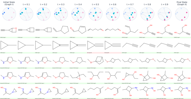
Figure 3: Geodesic interpolation in hyperbolic latent space between molecular graphs. Top row shows 10-step latent transitions with 2D-projected node embeddings. Lower rows decode these into molecules, with source and target at ends. Green labels mark valid intermediates; red indicates invalid ones. Chemical formulas and ring counts are annotated.

4.6 Discussion

Results.

Our results show that, (A1): Hyperbolic latent can help to enable near-perfect reconstruction of the original graphs. (A2): Hyperbolic generative models excel on datasets with strong hierarchical structure, such as Ego-Small and Community-Small, where they outperform Euclidean baselines. (A3): However, on molecular graphs like QM9, the advantage is less pronounced, likely due to their inherently Euclidean nature and weaker hierarchical patterns. (A4): Interpolations yield smooth structural and compositional transitions between molecules.

The findings suggest that hyperbolic latent spaces are particularly effective for domains with clear hierarchy. For Limitations and Future Work, please refer to Appendix E.

5 Conclusion

In this work, we have introduced GGBall, a novel framework for graph generation that leverages hyperbolic geometry to naturally encode the hierarchical structure of complex networks. By combining a vector-quantized autoencoder with Riemannian flow matching in the Poincaré ball, our approach enables curvature-aware and one-shot graph generation. Extensive experiments on both abstract and molecular graph benchmarks validate the effectiveness of our method, showing consistent improvements in reconstruction accuracy and distributional fidelity over Euclidean and graph-space baselines. Our findings highlight the potential of non-Euclidean generative models to accelerate scientific discovery across chemistry, biology, and network science, including applications such as materials design, molecular modeling, and complex graph generation.

Appendix A Notation in this paper

Table 4: Notations used in this paper.

Notation	Description
$\mathcal{M}$	Manifold
$\mathfrak{g}$	Metric
$\mathbb{R}$	Real number field
$\bm{x}$	Point on manifold
$c$	Absolute value of curvature
$\mathbb{B}$	Poincaré ball
$h$	Point on latent space
$\langle,\rangle_{c}$	Remannian inner product
$G$	A graph
$\mathcal{X}$	Set of graph nodes
$\mathcal{E}$	Set of graph edges
$\mathcal{T}$	Tangent space of a manifold
$m$	Number of nodes
$n$	Number of dimension for a specific space

Appendix B Related Works

B.1 Hyperbolic Graph Representation

Lorentz Model.

The Lorentz model represents hyperbolic space as part of a two-sheeted hyperboloid in Minkowski space, enabling efficient geodesic computation and optimization (Busemann, 1955; Ratcliffe, 2006; Epstein and Penner, 1987). It effectively captures hierarchical structures in graphs through continuous embeddings (Nickel and Kiela, 2018), and Lorentz transformations improve knowledge graph embeddings with fewer parameters (Liang et al., 2024). Hyperbolic Graph Convolutional Networks (HGCNs) have shown great potential in capturing hierarchical structures in graphs (Chami et al., 2019). Lorentzian Graph Convolutional Networks (LGCNs) enforce hyperbolic constraints, reducing distortion in tree-like graph representations (Zhang et al., 2021). Further advancements in hyperbolic geometry have enhanced neural architectures for better expressivity and efficiency (Fu et al., 2024; Ermolov et al., 2022; Ding et al., 2023; Yang et al., 2024).

Poincaré Ball Model.

The Poincaré ball models hyperbolic space within a unit ball, supporting compact embeddings for hierarchical data (Nickel and Kiela, 2017). Geometry-aware neural layers improve performance in tasks like link prediction and classification (Ganea et al., 2018). MuRP applies Möbius transformations for relation-specific knowledge graph embeddings (Balažević et al., 2019), and fully convolutional networks capture multi-scale graph features (Lensink et al., 2022). Core components like attention and convolution have been extended to the Poincaré ball for improved efficiency and stability (Shimizu et al., 2020), followed by a fully hyperbolic residual network that enhances robustness to distributional shifts and adversarial perturbations (Van Spengler et al., 2023). Unlike prior work that focuses on discriminative tasks, our framework leverages the Poincaré ball for generative modeling—specifically, learning and sampling discrete graph structures via a hyperbolic latent space. This extends the utility of hyperbolic geometry from representation learning to structured data generation.

B.2 Graph Generation

Autoencoder-Based Models.

Autoencoder-based models use latent representations to generate graphs. VAEs (Kingma et al., 2013) and VQVAEs (Van Den Oord et al., 2017; Razavi et al., 2019) are foundational in this area. JT-VAE builds molecular graphs by first generating a tree of substructures, then assembling them with message passing (Jin et al., 2018). Combining VAEs with graph transformers improves scalability and interpretability (Mitton et al., 2021). VQVAEs like VQ-T2G support text-conditioned graph generation by learning discrete latent codes aligned with textual prompts (Walker et al., 2021). Our model extends prior autoencoder-based approaches by using a hyperbolic latent space to better capture hierarchy and improve generative quality.

Autoregressive Models.

Autoregressive models generate graphs by sequentially adding nodes and edges. GraphRNN models the conditional distribution of graph structures using an RNN, producing diverse graphs (You et al., 2018). GRAN improves efficiency by incorporating attention and generating graph blocks (Liao et al., 2019). G2PT adopts transformer-based next-token prediction for goal-oriented graph generation and property prediction (Chen et al., 2025). In contrast, our method avoids sequential generation in graph space, which requires an explicit ordering, and instead enables one-shot decoding with stronger inductive bias for hierarchical structures.

Diffusion Models.

Diffusion models are effective for graph generation by transforming noise into structured graphs through a diffusion process. DiGress uses a discrete denoising diffusion model with a graph transformer to handle categorical node and edge attributes, achieving strong results (Vignac et al., 2023). DisCo extends this by modeling diffusion in a discrete-state continuous-time setting, balancing quality and efficiency while preserving graph discreteness (Xu et al., 2024).

Flow Matching.

Flow matching methods learn deterministic transport maps to transform simple distributions into complex graph structures. The Flow Matching framework trains continuous normalizing flows by regressing vector fields along fixed probability paths without simulation (Lipman et al., 2022). DeFoG adapts this to discrete graphs, separating training and sampling for improved flexibility (Qin et al., 2024). CatFlow frames flow matching as variational inference, enabling efficient generation of categorical data (Eijkelboom et al., 2024). In materials science, FlowMM applies Riemannian flow matching to generate high-fidelity materials, showing the method’s broad applicability (Miller et al., 2025). Building on these advances, we extend flow matching to a hyperbolic latent space, enabling geometry-aware graph generation with improved alignment to hierarchical structures.

Appendix C Algorithms

Algorithm 1 Hyperbolic $k$-Means Clustering

1:Samples $\{\bm{z}_{i}\in\mathbb{B}_{c}^{d}\}_{i=1}^{N}$, cluster count $K$, iterations $T$

2:Codebook $\{\bm{c}_{j}\in\mathbb{B}_{c}^{d}\}_{j=1}^{K}$, cluster sizes $\{n_{j}\}_{j=1}^{K}$

3:Initialize $\bm{c}_{j}^{(0)}\leftarrow\text{sample\_vectors}(\{\bm{z}_{i}\},K)$ $\triangleright$ Random initial centers

4:for $t=1$ to $T$ do

5:  Compute pairwise distances: $d_{ij}=-d_{c}^{2}(\bm{z}_{i},\bm{c}_{j}^{(t-1)})$  (Eq. 14)

6:  Assign clusters: $b_{i}\leftarrow\text{argmax}_{j}d_{ij},\ \forall i$

7:  Count clusters: $n_{j}\leftarrow|\{i:b_{i}=j\}|,\ \forall j$

8:  for $j=1$ to $K$ do

9:   if $n_{j}=0$ then

10:     $\bm{c}_{j}^{(t)}\leftarrow\bm{c}_{j}^{(t-1)}$  $\triangleright$ Retain dead clusters

11:   else

12:     $\bm{c}_{j}^{(t)}\leftarrow\text{WeightedMidpoint}(\{\bm{z}_{i}\},\mathbb{I}[b_{i}=j])$

13:     $\bm{c}_{j}^{(t)}\leftarrow\text{proj}_{\mathbb{B}_{c}^{d}}(\bm{c}_{j}^{(t)})$  $\triangleright$ Manifold projection

14:   end if

15:  end for

16:  if $\max_{j}d_{c}(\bm{c}_{j}^{(t)},\bm{c}_{j}^{(t-1)})<\epsilon$ then break

17:  end if

18:end for

Algorithm 2 Flow Matching for Graph Generation

1:Pretrained VQVAE with hyperbolic latent space, flow-based model

2:Generated graph $G_{\text{gen}}$

3:Sample latent codes from the standard normal distribution in hyperbolic space:

4:     $z_{0}\sim\mathcal{N}(0,I)$

5:Apply flow transformation to move from the source distribution to the target distribution in the latent space:

6:     $z_{t}=\text{Flow}_{\theta}(z_{0},t)$  for $t\in[0,1]$

7:Quantize the latent code to the nearest codebook vector:

8:     $z_{q}=\arg\min_{c}d_{\mathbb{B}_{c}}(z_{t},c)$

9:Decode the quantized latent code back to a graph:

10:     $G_{\text{gen}}=D_{\psi}(z_{q})$

11:Return the generated graph $G_{\text{gen}}$

Algorithm 3 Hyperbolic Graph Autoencoder (HGAE)

1:Graph $G=(\mathbf{X},\mathbf{E})$, hyperbolic curvature $c$, layers $L$, margins $r_{\min},r_{\max}$

2:Encoding Stage

3:Compute structural and spectral features $\mathbf{S}$ (e.g., graph Laplacian eigenfeatures).

4:Preprocess attributes using Euclidean MLP:

5: $\mathbf{X}_{h}=\exp_{0}^{c}(\text{MLP}([\mathbf{X},\mathbf{S}]))$, $\quad\mathbf{E}_{h}=\exp_{0}^{c}(\text{MLP}(\mathbf{E}))$

6:Initialize hyperbolic embeddings: ${z}_{i}^{(0)}\leftarrow\text{GNN}_{\theta}(\mathbf{X}_{h},\mathbf{E}_{h})$.

7:for $l=1,\dots,L$ do

8:  Perform hyperbolic attention-based message passing:

9: ${z}_{i}^{(l)}\leftarrow\text{Attention}_{\theta}({z}_{i}^{(l-1)})$

10:end for

11:Obtain final embeddings: ${Z}=\{{z}_{i}^{(L)}\}$.

12:Decoding Stage

13:for each node $i$ do

14:  Project hyperbolic embedding to tangent space:

15: $\log_{0}^{c}({z}_{i}^{(L)})\in T_{0}\mathbb{B}_{c}^{n}$

16:  Predict node attributes:

17: $p_{\phi}(\mathbf{x}_{i}|{z}_{i}^{(L)})=\text{Softmax}(\text{MLP}(\log_{0}^{c}({z}_{i}^{(L)})))$

18:end for

19:for each edge $(i,j)$ do

20:  Compute hyperbolic geometric features:

21: $f_{ij}=[\log_{0}^{c}({z}_{i}^{(L)}),\log_{0}^{c}({z}_{j}^{(L)}),\log_{{z}_{i}^{(L)}}^{c}({z}_{j}^{(L)}),d_{c}({z}_{i}^{(L)},{z}_{j}^{(L)}),\cos\theta_{ij}]$

22:  Predict edge attributes:

23: $p_{\phi}(e_{ij}|{z}_{i}^{(L)},{z}_{j}^{(L)})=\text{Softmax}(\text{MLP}(f_{ij}))$

24:end for

25:return Final embeddings ${Z}$, trained encoder-decoder

Algorithm 4 Hyperbolic Vector Quantized Variational AutoEncoder (HVQVAE)

1:Dataset $\mathcal{D}$, codebook size $K$, hyperbolic curvature $c$, EMA parameter $\beta$, margins $r_{\min},r_{max}$

2:Initialization

3:Initialize hyperbolic codebook $\mathcal{C}=\{c_{j}\}_{j=1}^{K}\subset\mathbb{B}_{c}^{d}$ using hyperbolic k-means or random sampling.

4:Encoding and Quantization

5:for each data point $x\in\mathcal{D}$ do

6:  Obtain latent embedding $z=\text{Encoder}_{\phi}(x)\in\mathbb{B}_{c}^{d}$

7:  Quantize embedding to nearest codebook vector using hyperbolic distance:

8: $z_{q}=\arg\min_{c_{j}\in\mathcal{C}}d_{c}(z,c_{j})$

9:end for

10:Decoding

11:Reconstruct input from quantized embedding: $\hat{x}=\text{Decoder}_{\theta}(z_{q})$

12:EMA Codebook Update

13:for each codebook vector $c_{j}$ do

14:  Compute centroid $\mu_{j}$ from assigned latent vectors $z_{i}$:

15: $\mu_{j}=\frac{1}{2}\bigoplus_{c}\left(\frac{\sum_{i}w_{ij}\lambda_{z_{i}}^{c}z_{i}}{\sum_{i}|w_{ij}|(\lambda_{z_{i}}^{c}-1)},\frac{\sum_{i}w_{ij}z_{i}}{\sum_{i}|w_{ij}|}\right)$

16:  EMA update codebook vector using Einstein midpoint:

17: $c_{j}^{(t+1)}=\text{proj}_{\mathbb{B}_{c}^{d}}\left([c_{j}^{(t)},\beta]_{c}\oplus_{c}[\mu_{j},1-\beta]_{c}\right)$

18:end for

19:Dead Codes Revival

20:if a codebook vector $c_{j}$ has not been updated for long periods then

21:  Re-initialize codebook vector $c_{j}$ to a new vector sampled from $\mathbb{B}_{c}^{d}$.

22:end if

23:return Trained encoder, decoder, and hyperbolic codebook

Algorithm 5 Training HVQVAE

1:Dataset $\{G_{i}\}$ of graphs

2:Trained HVQVAE model on hyperbolic

3:Initialize hyperbolic encoder $E_{\phi}$, codebook $\mathcal{C}$, and decoder $D_{\psi}$

4:for each graph $G_{i}$ in the dataset do

5:  Map the graph’s node and edge features to the hyperbolic space via the Poincaré ball model:

6:       $Z_{i}=\text{Exp}_{0}(E_{\phi}(G_{i}))$ $\triangleright$ Exponential map to hyperbolic space

7:  Apply message passing and attention to encode information in latent space

8:  Quantize the latent code via the hyperbolic codebook $\mathcal{C}$:

9:       $z_{q}=\arg\min_{c}d_{\mathbb{B}_{c}}(z,c)$

10:  Decode the quantized latent codes back to the original graph structure:

11:       $\hat{G}_{i}=D_{\psi}(z_{q})$

12:  Update model parameters using the loss Eq. 40

13:end for

Appendix D Additional Technical Details

D.1 Remannian Manifold

A Riemannian manifold $(\mathcal{M},\mathfrak{g})$ is a smooth manifold $\mathcal{M}$ equipped with an inner product $\mathfrak{g}_{p}:T_{p}\mathcal{M}\times T_{p}\mathcal{M}\to\mathbb{R}$ on the tangent space $T_{p}\mathcal{M}$ at each point $p\in\mathcal{M}$, which varies smoothly with $p$. The inner product $g$ is called the Riemannian metric and induces a notion of distance and angle on the manifold.

Given a point $p\in\mathcal{M}$ and a tangent vector $v\in T_{p}\mathcal{M}$, the exponential map $\exp_{p}:T_{p}\mathcal{M}\to\mathcal{M}$ maps $v$ to the point reached by traveling along the geodesic starting at $p$ in the direction of $v$ for unit time. Conversely, the logarithmic map $\log_{p}:\mathcal{M}\to T_{p}\mathcal{M}$, when defined, maps a point $q\in\mathcal{M}$ back to the tangent vector at $p$ corresponding to the initial velocity of the geodesic from $p$ to $q$. These two maps allow the manifold geometry to be locally approximated using linear operations in the tangent space.

D.2 Hyperbolic Geometry

Let $(\mathcal{M},\mathfrak{g})$ be a complete, simply connected Riemannian manifold of constant sectional curvature $\kappa<0$. Then $(\mathcal{M},\mathfrak{g})$ is called the $n$-dimensional hyperbolic space with curvature $\kappa$, denoted $\mathbb{H}^{n}_{\kappa}$. Up to isometry, there exists a unique such space for each dimension $n$ and curvature $\kappa$, making hyperbolic space a canonical example of a negatively curved space form in Riemannian geometry.

In practice, several coordinate models are commonly used to represent this manifold in different ambient geometries. These include the Lorentz model, the Poincaré ball model, and the Beltrami–Klein model. Although their coordinate expressions differ, these models are all isometric to one another and describe the same underlying hyperbolic space. Closed-form mappings exist between the models, allowing flexibility in geometric computation.

We summarize below the Riemannian metrics associated with each of these models.

Lorentz Model.

This model is realized as a hypersurface embedded in $(n{+}1)$-dimensional Minkowski space $\mathbb{R}_{1}^{n+1}$ equipped with the Lorentzian inner product:

$$\langle\mathbf{x},\mathbf{y}\rangle_{\mathcal{L}}=\mathbf{x}^{\top}\mathfrak{g}_{\mathcal{L}}\mathbf{y},\quad\text{where}\quad\mathfrak{g}_{\mathcal{L}}=\mathrm{diag}(-1,1,\dots,1).$$

Poincaré Ball Model.

Defined on the open ball $\mathbb{B}_{c}^{n}=\{\mathbf{x}\in\mathbb{R}^{n}\mid c\|\mathbf{x}\|^{2}<1\}$ and here $c=-\kappa$.The Poincaré model uses a conformal metric:

$$\mathfrak{g}_{\mathbf{x}}^{c}=\lambda_{\mathbf{x}}^{2}I_{n},\quad\text{with}\quad\lambda_{\mathbf{x}}=\frac{2}{1-c\|\mathbf{x}\|^{2}}.$$

Beltrami–Klein Model.

Also defined on the same open ball, the Beltrami–Klein model uses a non-conformal metric. Unlike the Poincaré model, it does not preserve angles, but has the advantage that geodesics are represented as straight lines within the Euclidean ball:

$$\hat{\mathfrak{g}}_{\mathbf{x}}^{c}=(1-c\|\mathbf{x}\|^{2})^{-1}I_{n}+(1-c\|\mathbf{x}\|^{2})^{-2}c\,\mathbf{x}\mathbf{x}^{\top}.$$

These models provide flexible choices for representing hyperbolic geometry depending on the task at hand, including optimization, inference, and geometric embedding in machine learning applications. Poincaré ball here is preferred in graph embedding because it preserves local angles (conformal), naturally encodes hierarchy near the boundary, and supports efficient optimization in a bounded Euclidean space.

D.3 Graphs in Hyperbolic Space

Previous works (Sarkar, 2011; Fu et al., 2024) have suggested that graph features are well-suited for embedding in hyperbolic space due to its tree-like structure Coornaert et al. (2006).

Theorem 1.

(de Gromov’s approximation theorem) For any $\delta$-hyperbolic space, there exists a continuous mapping from the space to an $R$-Tree such that the distances between points are approximately preserved with a small error term. More formally, the mapping $\Phi:\mathcal{X}\rightarrow T$ satisfies the following distance preservation property:

$$|x-y|-2k\delta\leq|\Phi(x)-\Phi(y)|\leq|x-y|,$$

where $\mathcal{X}$ is the $\delta$-hyperbolic space, $T$ is the $R$-Tree, and $k$ is the number of sampled points in the mapping.

D.4 Basic Operations on Poincaré Ball

D.4.1 Möbius Addition and Transformations

Möbius addition is defined on Poincaré ball as follows:

$$\bm{x}\oplus_{c}\bm{y}=\frac{\left(1+2c\langle\bm{x},\bm{y}\rangle+c\|\bm{y}\|^{2}\right)\bm{x}+\left(1\bm{-}c\|\bm{x}\|^{2}\right)\bm{y}}{1\bm{+}2c\langle\bm{x},\bm{y}\rangle+c^{2}\|\bm{x}\|^{2}\|\bm{y}\|^{2}},$$ (10)

which reverse calculation is defined by

$$\quad\bm{x}\ominus_{c}\bm{y}=\bm{x}\oplus_{c}(\bm{-}\bm{y}).$$ (11)

This operation is closed on $\mathbb{D}^{n}$ and defines a non-associative algebraic structure known as a gyrogroup.

Unlike Euclidean addition, Möbius addition is not associative. Instead, it satisfies a weaker form of associativity known as gyroassociativity:

$$u\oplus(v\oplus_{c}w)=(u\oplus_{c}v)\oplus_{c}\text{gyr}[u,v](w),$$

Accordingly, when considering transformations on the Poincaré disk, it is important to account for the underlying non-associative gyrogroup structure. Throughout this work, all Möbius additions are consistently defined as left additions, which naturally gives rise to operations where composing with the inverse yields the identity transformation.

D.4.2 Logarithm Map, Exponential Map, and Geodesic Distance

The exponential map $\exp_{c}^{x}:\mathcal{T}_{x}\mathbb{B}_{c}^{n}\rightarrow\mathbb{B}_{c}^{n}$ is described in as follows:

$$\exp_{\bm{x}}^{c}\left(\bm{v}\right)=\bm{x}\oplus_{c}\frac{1}{\sqrt{c}}\tanh\left(\frac{\sqrt{c}\lambda_{\bm{x}}^{c}\|\bm{v}\|}{2}\right)[\bm{v}],\quad\forall\bm{x}\in\mathbb{B}_{c}^{n},\bm{v}\in\mathcal{T}_{\bm{x}}\mathbb{B}_{c}^{n}.$$ (12)

The logarithmic map $\log_{c}^{x}=(\exp_{c}^{x})^{-1}:\mathbb{B}_{c}^{n}\rightarrow\mathcal{T}_{x}\mathbb{B}_{c}^{n}$ provides the inverse operation:

$$\log_{\bm{x}}^{c}\left(\bm{y}\right)=\frac{2}{\sqrt{c}\lambda_{\bm{x}}^{c}}\tanh^{-1}\left(\sqrt{c}\|\ominus_{c}\bm{x}\oplus_{c}\bm{y}\|\right)[\ominus_{c}\bm{x}\oplus_{c}\bm{y}],\quad\forall\bm{x},\bm{y}\in\mathbb{B}_{c}^{n}.$$ (13)

Geodesic distance between $\bm{x},\bm{y}\in\mathbb{B}_{c}^{n}$ is defined as:

$$d_{c}\left(\bm{x},\bm{y}\right)=\frac{2}{\sqrt{c}}\tanh^{-1}\left(\sqrt{c}\|\ominus_{c}\bm{x}\oplus_{c}\bm{y}\|\right)=\|\log_{\bm{x}}^{c}(\bm{y})\|_{\bm{x}}^{c}.$$ (14)

Despite the noncommutative aspect of the Möbius addition $\oplus_{c}$, this distance function becomes commutative thanks to the commutative aspect of the Euclidean norm of the Möbius addition.

D.5 Hyperbolic Network Backbone

Prior efforts to construct hyperbolic neural networks predominantly leveraged the Lorentz model, yet its numerical instability (particularly the non-invertibility of exponential and logarithmic maps in high dimensions) limits scalability. In contrast, the Poincaré ball model offers superior numerical robustness and conformal structure, making it a pragmatic foundation for building deep architectures. Building on these insights, we unify and extend hyperbolic machine learning by developing a comprehensive suite of foundational components and mainstream network modules within the Poincaré framework.

D.5.1 Poincaré Multinomial Logistic Regression

Hyperbolic hyperplanes generalize Euclidean decision boundaries by constructing sets of geodesics orthogonal to a tangent vector $\bm{a}\in\mathcal{T}_{p}\mathbb{B}_{c}^{n}\setminus\{\bm{0}\}$ at a base point $\bm{p}$. However, traditional formulations suffer from over-parameterization of the hyperplane.  Shimizu et al. (2020) address this by proposing unidirectional hyperplanes, where the base point $\bm{q}_{k}$ is constrained as $\bm{q}_{k}=\exp_{0}^{c}(r_{k}[\bm{a}_{k}])$ using a scalar bias $r_{k}\in\mathbb{R}$. This reduces redundancy and stabilizes optimization. Building on this, hyperbolic multinomial logistic regression (MLR) generalizes Euclidean MLR by measuring distances to margin hyperplanes. For $K$ classes, the unidirectional hyperbolic MLR formulation for all $\bm{x}\in\mathbb{B}_{c}^{n}$ is defined as:

$$\bm{v}_{k}=p(y=k\mid\bm{x})\propto\operatorname{sign}\left(\langle-\bm{q}_{k}\oplus_{c}\bm{x},\bm{a}_{k}\rangle\right)\|\bm{a}_{k}\|d_{c}\left(\bm{x},\bar{H}_{\bm{a}_{k},r_{k}}^{c}\right),$$ (15)

where $d_{c}(\bm{x},\bar{H}_{\bm{a}_{k},r_{k}}^{c})$ denotes the hyperbolic distance from $\bm{x}$ to the $k$-th unidirectional hyperplane. $\bm{a}_{k}$ and $r_{k}$ are learnable parameters. This formulation preserves the interpretability of Euclidean margins while leveraging the exponential growth of hyperbolic space for hierarchical classification.

Poincaré Fully Connected layer.

The Poincaré fully connected (FC) layer generalizes Euclidean affine transformations to hyperbolic space while preserving geometric consistency. Following  Shimizu et al. (2020), we adopt a reparameterized formulation that circumvents the parameter redundancy inherent in earlier hyperbolic linear layers (Ganea et al., 2018). For an input $\bm{x}\in\mathbb{B}_{c}^{n}$, the layer computes the output $\bm{y}\in\mathbb{B}_{c}^{m}$ as:

$$\bm{y}=\mathcal{F}^{c}(\bm{x};\bm{Z},\bm{r}):=\bm{w}(1+\sqrt{1+c\|\bm{w}\|^{2}})^{-1},\mathrm{~where~}\bm{w}:=(c^{-\frac{1}{2}}\sinh\left(\sqrt{c}\,\bm{v}_{k}(\bm{x})\right))_{k=1}^{m}.$$ (16)

where $\bm{v}_{k}(\bm{x})$ denotes the signed hyperbolic distance from $\bm{x}$ to the unidirectional hyperplane $\bar{H}_{\bm{a}_{k},r_{k}}^{c}$ which is described in Eq. 15, derived via parallel transport and Möbius addition (Shimizu et al., 2020). This formulation ensures that each output dimension corresponds to a geometrically interpretable distance metric in $\mathbb{B}_{c}^{m}$, aligning with the intrinsic curvature of the manifold.

Poincaré Layernorm.

We introduce Poincaré LayerNorm, a novel normalization module that stabilizes training in hyperbolic networks while preserving geometric integrity. Unlike Euclidean LayerNorm, which operates directly on manifold coordinates, our method leverages the logarithmic map to project hyperbolic features $\bm{x}\in\mathbb{B}_{c}^{n}$ to the tangent space at the origin $\mathcal{T}_{0}\mathbb{B}_{c}^{n}$. Here, standard LayerNorm is applied to the Euclidean-flattened features, followed by an exponential map to reproject the normalized result back to $\mathbb{B}_{c}^{n}$. Formally, for input $\bm{x}$:

$$\bm{x}_{norm}=\exp_{0}^{c}(\text{LayerNorm}(\log_{0}^{c}(\bm{x}))),$$ (17)

where weights and biases in the LayerNorm submodule are initialized to minimize distortion. This approach decouples normalization from manifold curvature, ensuring stable gradient propagation without violating hyperbolic geometry.

Poincaré ResNet.

For deep hyperbolic architectures, we adapt residual connections to mitigate vanishing gradients, inspired by  Chami et al. (2019). Given a hyperbolic feature $\bm{x}\in\mathbb{B}_{c}^{n}$ and a nonlinear transformation $\mathcal{F}(\bm{x})$, the Poncaré ResNet block computes:

$$\bm{x}_{out}=\bm{x}\oplus_{c}\mathcal{F}(\bm{x}),$$ (18)

D.5.2 Poincaré Graph Neural Networks

We introduce a Poincaré ball-based graph neural network (GNN) that generalizes message passing to hierarchical graph structures. Unlike Lorentz-based approaches that operate on hyperboloid coordinates, our architecture leverages the conformal structure of the Poincaré ball to enable stable gradient propagation and efficient hyperbolic-linear operations. Let $\bm{H}_{X}=\{\bm{h}_{i}\in\mathbb{B}_{c}^{n}\}_{i=1}^{N}$ denote node features and $\bm{H}_{E}=\{\bm{h}_{ij}\in\mathbb{B}_{c}^{n}\}_{(i,j)\in\mathcal{E}}$ edge features. Our architecture cooperates via two geometrically consistent phases:

Hyperbolic Message Passing and Edge Update.

For each edge $(i,j)$, compute adaptive shift and scale parameters from the hyperbolic distance $d_{c}(\bm{h}_{i}^{l},\bm{h}_{j}^{l})$:

$$\bm{\gamma}_{ij}^{l},\bm{\beta}_{ij}^{l}=\text{Linear}(d_{c}(\bm{h}_{i}^{l},\bm{h}_{j}^{l}))$$ (19)

where $\text{Linear}:\mathbb{R}^{d}\rightarrow\mathbb{R}^{2d}$ ensures scale-awareness. Project $\bm{h}_{i}^{x}$, $\bm{h}_{j}^{x}$ and $\bm{h}_{ij}^{e}$ to $\mathcal{T}_{0}\mathbb{B}_{c}^{n}$ via $\log_{0}^{c}(\cdot)$, concatenate, and modulate to update the message:

$$\bm{m}_{i}^{l+1}=\sum_{j\in\mathcal{N}(i)}\underbrace{\text{AdaLN}\left(\mathcal{W}_{e}\left[\log_{0}^{c}(\bm{h}_{i}^{l}),\log_{0}^{c}(\bm{h}_{j}^{l}),\log_{0}^{c}(\bm{h}_{ij}^{l})\right],\bm{\gamma}_{ij}^{l},\bm{\beta}_{ij}^{l}\right)}_{\bm{m}_{ij}^{l+1}},$$ (20)

where $\mathcal{W}_{e}\in\mathbb{R}^{3n\times n\times d}$ is a Euclidean linear layer. We can get a new edge representation by pulling the message back up to the Poincaré manifold.

$$\bm{h}_{ij}^{l+1}=\exp_{0}^{c}\left(\bm{m}_{ij}^{l+1}\right)$$ (21)

Hyperbolic Node Aggregation.

For node $i$, we have aggregated messages $\bm{m}_{i}^{l+1}$ from neighbors $\mathcal{N}(i)$ in Eq. 20. Similarly, we compute adaptive shift and scale parameters $\bm{\eta}_{i}^{l+1},\bm{\zeta}_{i}^{l+1}$ from the message and update node features:

$$\bm{h}_{i}^{l+1}=\exp_{0}^{c}\left(\log_{0}^{c}(\bm{h}_{i}^{l})+\text{AdaLN}\left(\mathcal{W}_{x}\left[\log_{0}^{c}(\bm{h}_{i}^{l}),\log_{0}^{c}(\bm{m}_{i}^{l+1})\right],\bm{\eta}_{i}^{l+1},\bm{\zeta}_{i}^{l+1}\right)\right)$$ (22)

with $\mathcal{W}_{e}\in\mathbb{R}^{2n\times n\times d}$ as Euclidean linear layer.

D.5.3 Poincaré Transformers

We present a hyperbolic transformer architecture that extends self-attention mechanisms to the Poincaré ball model while preserving geometric consistency. Given the hidden feature $\bm{H}=\{\bm{h}_{i}\in\mathbb{B}_{c}^{n}\}_{i=1}^{N}$, the transformer first injects positional information via Möbius addition of learnable hyperbolic embeddings. The sequence then passes through $L$ identical layers, which containing Poincaré Multi-Head Attention and Poincaré Feed-Forward Network. Both components employ residual connections with Möbius addition and Poincaré LayerNorm.

Poincaré Attention Mechanisms.

The attention mechanism generalizes scaled dot-product attention to hyperbolic space through three stages:

Projection & Splitting.

Inputs are projected into queries $\bm{Q}$, keys $\bm{K}$, and values $\bm{V}$ via Poincaré FC layers (Eq. 15). As described in Shimizu et al. (2020), we use $\beta$-splitting to split each tensor into $h$ heads:

$$\bm{Q}_{i},\bm{K}_{i},\bm{V}_{i}=\text{Split}_{c}(\bm{Q}),\text{Split}_{c}(\bm{K}),\text{Split}_{c}(\bm{V}),$$ (23)

where $\text{Split}_{c}$ scales dimensions via beta functions.

Geodesic Attention Score.

Attention weights are computed using hyperbolic distance to maintain the hyperbolic geometry structure, which can be formulated as:

$$\alpha_{ij}=\text{softmax}(\tau d_{c}(\bm{Q}_{i},\bm{K}_{i})-\gamma),$$ (24)

where $\tau$ is an inverse temperature and $\gamma$ is a bias parameter, which was proposed by Gulcehre et al. (2019). After applying a similarity function and obtaining each weight, the values are aggregated by Möbius gyromidpoint:

$$\bm{Z}_{i}=\sum_{j=1}^{T}\left[\bm{V}_{j},\alpha_{ij}\right]_{c}:=\frac{1}{2}\otimes_{c}\left(\frac{\sum_{j}\alpha_{ij}\lambda_{c}^{V_{j}}\bm{V}_{j}}{\sum_{j}|\alpha_{ij}|(\lambda_{c}^{V_{j}}-1)}\right),$$ (25)

the symbol $\frac{1}{2}\otimes_{c}\underline{\bm{x}}=\frac{\underline{\bm{x}}}{1+\sqrt{1-c\|\underline{\bm{x}}\|^{2}}}$, which is described in  Ungar (2008).

Multi-Head Composition.

Head outputs $\{\bm{Z}_{i}\}_{i=1}^{h}$ are combined via $\beta$-concatenation and out projection:

$$\bm{O}=\text{Concat}_{c}(\bm{Z}_{1},...,\bm{Z}_{h})\oplus_{c}\mathcal{W}_{O},$$ (26)

where $\mathcal{W}_{O}$ is a Poincaré linear projection and $\text{Concat}_{c}$ inversely scales beta ratios from splitting.

Time-aware Transformer Layers.

To integrate temporal dynamics into hyperbolic diffusion processes, we extend the Poincaré transformer with adaptive time-conditioned modulation. Each layer injects timestep embeddings $\bm{t}_{emb}\in\mathbb{R}$ through Euclidean affine transformations of normalized features. Following Euclidean Diffusion Transformer (Peebles and Xie, 2023), we regress time-conditioned gate $\bm{\alpha}_{ij}^{l}$, shift $\bm{\beta}_{ij}^{l}$, and scale $\bm{\gamma}_{ij}^{l}$ parameters from $\bm{t}_{emb}$:

$$\bm{\alpha}_{attn}^{l},\bm{\beta}_{attn}^{l},\bm{\gamma}_{attn}^{l},\bm{\alpha}_{ffn}^{l},\bm{\beta}_{ffn}^{l},\bm{\gamma}_{ffn}^{l},=\text{Linear}(\bm{t}_{emb})$$ (27)

where $\text{Linear}:\mathbb{R}^{n\times d}\rightarrow\mathbb{R}^{6n\times d}$ is Euclidean linear layer. These parameters drive an AdaLN modulation mechanism and modulated feature representation $\bm{h}_{new}$ is computed as:

$$\bm{h}_{new}=\bm{h}\oplus_{c}\left[\bm{\alpha}_{ij}^{l}\cdot\text{PoincareAttention}(\exp_{0}^{c}(\text{AdaLN}(\log_{0}^{c}(\bm{h}),\bm{\beta}_{ij}^{l},\bm{\gamma}_{ij}^{l})))\right],$$ (28)

where $\text{AdaLN}(\cdot)$ is the similar function in Diffusion Transformer (Peebles and Xie, 2023). Subsequently, $\bm{h}_{new}$ is processed similarly in the Poincaré Feed-Forward Networks, forming a complete Time-aware Transformer Layer, and we use $L$ Time-aware Transformer Layers to construct Poincaré Diffusion Transformer used in Section 3.3.

In all the above networks, we ensure that outputs remain within the Poincaré disk, capitalizing on the inherent non-linearity of Poincaré linear transformations. This approach obviates the need for conventional non-linear activation functions, as the hyperbolic geometry inherently captures and models complex, hierarchical relationships.

D.6 Hyperbolic AutoEncoder for Graph

D.6.1 Hyperbolic Graph AutoEncoder (HGAE)

Graph autoencoders are unsupervised learning methods designed to learn low-dimensional representations of graphs. In hyperbolic space, graph autoencoders can more effectively capture the hierarchical structure of graphs. Our Hyperbolic Graph Autoencoder (HGAE) consists of a hyperbolic encoder and a hyperbolic decoder. The encoder maps graph nodes to points in hyperbolic space, while the decoder reconstructs the adjacency matrix of the graph.

Graph Encoder.

The encoder first incorporates extra structural and spectral graph features—eigenvectors and eigenvalues of the graph Laplacian—to enrich global topological awareness. Such features boost the expressive capacity of graph neural networks and are helpful for training a powerful autoencoder structure (Vignac et al., 2023; Beaini et al., 2021). Since these features are not exposed to the graph generation process, we could theoretically construct any features that can increase the expressiveness of graphs. These features undergo initial Euclidean preprocessing via multilayer perceptrons (MLPs), ensuring effective fusion of multidimensional attributes. The result is mapped onto the Poincaré ball with an origin-centred exponential map:

$$\mathbf{X}_{h}=\exp_{0}\!\bigl{(}\mathrm{MLP}([\mathbf{X},\mathbf{S}])\bigr{)},\qquad\mathbf{E}_{h}=\exp_{0}\!\bigl{(}\mathrm{MLP}(\mathbf{E})\bigr{)}$$ (29)

Subsequent hyperbolic graph neural network (GNN) layers aggregate localized structural patterns, while $L$ hyperbolic Transformer layers propagate information globally, yielding final hyperbolic embeddings $\mathbf{z}_{i}=\mathbf{h}_{i}^{L}\in\mathbf{H}^{D}$ that preserve multiscale structural semantics.

$$\mathbf{h}_{i}^{l+1}=\mathrm{Attention}_{\theta}(\mathbf{h}_{i}^{l}),\qquad\mathbf{h}^{0}=\mathrm{GNN}_{\theta}(\mathbf{X}_{h},\mathbf{E}_{h})$$ (30)

Probabilistic Graph Decoder.

The decoder architecture operates under the conditional independence assumption, where node attributes depend solely on their respective embeddings, while edge connectivity and features are conditionally dependent on node pairs. This factorization yields the joint reconstruction probability:

$$p_{\phi}(\mathbf{X},\mathbf{E}\mid\mathbf{H})=\prod_{i=1}^{n}p_{\phi}(\mathbf{x}_{i}\mid\mathbf{h}_{i})\prod_{j=1}^{n}\prod_{k=1}^{n}p_{\phi}(\mathbf{e}_{jk}\mid\mathbf{h}_{j},\mathbf{h}_{k})$$ (31)

We first feed the latent repsentations $\mathbf{z}_{i}$ into a 2 layer Poincaré self attention model, to allow full interaction between nodes, and obtain node-level representations $\mathbf{h}_{i}$. For attribute reconstruction, we first project the hyperbolic feature on to $\mathcal{T}_{0}\mathbb{B}_{c}^{n}$, and then apply a Euclidean MLP-based prediction head followed by Softmax distribution.

$$p_{\phi}(\mathbf{x}_{i}\!\mid\!\mathbf{h}_{i})=\mathrm{Softmax}\mathrm{MLP}_{\phi}\left(\log_{0}^{c}(\bm{h}_{i})\right)$$ (32)

Edge probabilities are derived from a comprehensive set of hyperbolic geometric features:

$$\mathbf{f}_{ij}=\left[\log_{\mathbf{0}}^{c}(\mathbf{h}_{i}),\log_{\mathbf{0}}^{c}(\mathbf{h}_{j}),\log_{\mathbf{h}_{i}}^{c}(\mathbf{h}_{j}),d_{c}(\mathbf{h}_{i},\mathbf{h}_{j}),\cos\theta_{ij}\right]$$ (33)

where the log-map vectors represents the directional relationship in the tangent space, $d_{c}\left(\bm{h}_{i},\bm{h}_{j}\right)$ computes the explicit hyperbolic distance encoding hierarchical relationships, and $\theta_{ij}=\angle_{\mathbb{H}}(0,\bm{h}_{i},\bm{h}_{j})$ captures relative angular positions The resulting $\mathcal{R}^{3D+2}$ feature vector is processed through an MLP with softmax output to predict:

$$p_{\phi}(\mathbf{e}_{ij}\mid\mathbf{h}_{i},\mathbf{h}_{j})=\mathrm{Softmax}\left(\mathrm{MLP}_{\phi}(\mathbf{f}_{ij})\right)$$ (34)

Reconstruction Loss.

By jointly optimizing feature and topological reconstruction under hyperbolic geometric constraints, the model ensures latent embeddings retain both structural hierarchy and attribute-node relationships, outperforming conventional Euclidean counterparts in preserving complex graph semantics.

$$\mathcal{L}_{\text{AE}}=\lambda_{\text{node}}\;\mathcal{L}_{\text{node}}\;+\;\lambda_{\text{edge}}\;\mathcal{L}_{\text{edge}}\;+\;\lambda_{\text{reg}}\;\mathcal{L}_{\text{reg}},$$ (35)

$$\mathcal{L}_{\text{node}}=-\;\mathbb{E}_{(\mathbf{X},\mathbf{E})\sim\mathcal{D}}\;\mathbb{E}_{\mathbf{h}\sim p_{\theta}(\mathbf{h}\mid\mathbf{X},\mathbf{E})}\sum_{i=1}^{n}\sum_{c=1}^{d_{1}}x_{ic}\,\log p_{\phi}(x_{ic}=1\mid\mathbf{h}_{i}).$$ (36)

$$\mathcal{L}_{\text{edge}}=-\;\mathbb{E}_{(\mathbf{X},\mathbf{E})\sim\mathcal{D}}\;\mathbb{E}_{\mathbf{h}\sim p_{\theta}(\mathbf{h}\mid\mathbf{X},\mathbf{E})}\sum_{i=1}^{n}\sum_{j=1}^{n}\sum_{c=1}^{d_{2}}e_{ijc}\,\log p_{\phi}(e_{ijc}=1\mid\mathbf{h}_{i},\mathbf{h}_{j}).$$ (37)

With edge reconstruction loss, node reconstruction loss, and regularization loss, and lambda being hyperparameters.

Training instability remains a fundamental challenge in hyperbolic neural networks, primarily due to the exponential growth of hyperbolic distance as points move away from the origin toward the Poincaré ball boundary. Empirical observations reveal that embeddings with small norms (e.g., below 0.1) exhibit near-Euclidean behavior, while those approaching the boundary (norms > 0.8) frequently suffer from gradient instability during optimization. To mitigate this issue, we adopt an adaptive regularization approach inspired by recent advances in clipped hyperbolic representations. Unlike hard constraints that strictly enforce norm boundaries, we introduce a band loss composed of two hinge loss terms, which softly encourages hyperbolic embeddings $\mathrm{h}_{i}$ to remain within a stable intermediate region.

$$\mathcal{L}_{\text{band}}=\;\frac{1}{n}\;\sum_{i=1}^{n}\Bigl{[}\bigl{(}\max\{0,\;\lVert\mathbf{z}_{i}\rVert-r_{\max}\}\bigr{)}^{2}+\;\bigl{(}\max\{0,\;r_{\min}-\lVert\mathbf{z}_{i}\rVert\}\bigr{)}^{2}\Bigr{]}$$ (38)

Where we set the inner margin $r_{min}=0.2$, and the outer margin $r_{max}=0.8$

D.6.2 Hyperbolic Variational AutoEncoder (HVAE)

Variational Auto-Encoders augment a classic auto-encoder with a probabilistic KL penalty, helping to reduce the high-variance in latent space and enable sampling. In hyperbolic space $\mathbb{H}^{n}$, the Euclidean Gaussian is no longer appropriate, so we adopt the Wrapped Normal distribution (Mathieu et al., 2019; Grattarola et al., 2019; Nagano et al., 2019), for both prior and posterior:

$$p(\mathbf{z}_{i})=\mathcal{N}_{\mathbb{H}}(\mathbf{0},\Sigma),\qquad q_{\phi}(\mathbf{z}_{i}\mid\mathbf{X},E)=\mathcal{N}_{\mathbb{H}}\!\bigl{(}\bm{\mu}_{\phi}(\mathbf{x}),\;\bm{\Sigma}_{\phi}(\mathbf{x})\bigr{)}.$$ (39)

where $\bm{\mu}=\text{PoincareLinear}\left(h_{i}\right)\in\mathbb{B}_{c}^{n}$, $\Sigma=\text{Softplus}\Big{(}\text{Linear}\left(\log_{0}^{c}\left(h_{i}\right)\right)\Big{)}\in\mathbb{R}^{n}_{+}$. We choose the prior standard deviation be isotropic and renormalized by the square root of the dimension of hyperbolic space, $\Sigma=\frac{1}{\sqrt{d}}\mathbf{I}$, to ensure sampled points don’t get pushed to the boundary as dimensionality increases.

Reconstruction Loss.

HVAE is trained by maximising the evidence lower bound, or equivalently minimising $\mathcal{L}_{\text{VAE}}=\mathbb{E}_{q_{\phi}}\bigl{[}-\log p_{\theta}(\mathbf{x},\mathbf{e}\mid\mathbf{z})\bigr{]}+\beta\,\mathrm{KL}\!\bigl{(}q_{\phi}(\mathbf{z}\mid\mathbf{x},\mathbf{e})\;\|\;p(\mathbf{z})\bigr{)},$ where the lambda term controls the reconstruction-generation trade-off (Higgins et al., 2017). Since closed-form solutions for these distributions are unavailable, we compute the KL term via Monte Carlo estimation.

We have also implemented a hyperbolic variational autoencoder (HVAE), using the wrapped normal distribution as the prior in latent space, and tested the reconstruction performance. However, we observe that sampling in high-dimensional hyperbolic space is highly unstable, and Monte Carlo estimation of the KL divergence often leads to numerical instability. As a result, the HVAE significantly underperforms in both reconstruction and generation tasks compared to HAE and HVQVAE.

D.6.3 Hyperbolic Vector Quantized Variational AutoEncoder (HVQVAE)

We introduce a hyperbolic vector quantized variational autoencoder (HVQVAE) that discretizes latent representations while preserving hierarchical structure.

Hyperbolic Codebook.

We propose a novel hyperbolic codebook that resides entirely within the Poincaré disk, ensuring all operations remain consistent with the hyperbolic geometry.

Codebook Initialization.

The hyperbolic codebook $\mathcal{C}\in\mathbb{B}_{c}^{n}$ is initialized via manifold-aware random sampling or optimized through hyperbolic $k$-means clustering. This algorithm uses initial vectors are drawn from the Poincaré neural network, ensuring uniform coverage across hierarchical scales and minimizes the sum of squared geodesic distance, which is defined as Eq. 14. The algorithm terminates when the centroid movement after 10 iterations (Alg. 18). We choose random initialization which achieves a slightly better results, while K-means initialization method often offers a faster convergence,

Quantization Method.

In the Poincaré VQVAE, quantization maps an input embedding $\bm{Z}\in\mathbb{B}_{c}^{n}$ to the nearest codebook vector using the hyperbolic geodesic distance. Formally, the quantized embedding $\mathbf{z}_{q}$ is obtained by selecting the codebook vector $\mathbf{c}_{i}$ that minimizes the geodesic distance.

Loss Function.

The training objective combines three geometrically consistent components:

$$\mathcal{L}_{\text{HVQVAE}}=\lambda_{1}\underbrace{\mathbb{E}_{p_{\phi}}\bigl{[}-\log p_{\theta}(\bm{x},\bm{e}\mid\bm{z}_{q})\bigr{]}}_{\text{Reconstruction}}+\lambda_{2}\underbrace{\mathbb{E}_{z}[d_{c}^{2}(\text{sg}(\bm{z}_{q}),\bm{z})]}_{\text{Commitment}}+\lambda_{3}\underbrace{\mathbb{E}_{z}[d_{c}^{2}(\bm{z}_{q},\text{sg}(\bm{z}))]}_{\text{Consistency}},$$ (40)

where reconstruction loss is same as VAE; commitment loss anchors latent codes to quantized vectors, and Codebook loss updates embeddings via straight-through gradient estimation $\text{sg}(\cdot)$. It is worth noting that since the hyperbolic codebook is in hyperbolic space and the model parameters are in Euclidean space, we use both a Riemannian optimizer and a traditional optimizer, and the same is true for the positional encoding in Transformer.

Hyperbolic Exponential Moving Average.

To stabilize training and avoid mode collapse, we incorporate Hyperbolic Exponential Moving Average (EMA) for codebook updates.

EMA Update.

Codebook vectors $\bm{c}_{j}\in\mathbb{B}_{c}^{n}$ update via Riemannian EMA to balance historical states and new features. We compute a new centroid $\bm{\mu}_{j}$ from assigned samples $\bm{z}_{i}$ with weights $w_{ij}=\mathbb{I}(\bm{z}_{i}\rightarrow\bm{c}_{j})$, which is an indicator function that assigns a weight of 1 when the sample $\bm{z}_{i}$ is mapped to the codebook vector $\bm{c}_{j}$ and 0 otherwise:

$$\bm{\mu}_{j}=\frac{1}{2}\otimes_{c}\left(\frac{\sum_{i=1}^{N}w_{ij}\lambda_{c}^{\bm{z}_{i}}\bm{z}_{i}}{\sum_{i=1}^{N}|w_{ij}|(\lambda_{c}^{\bm{z}_{i}}-1)}\right)$$ (41)

Similarly, we can update codebook vectors via Einstein midpoint (Ungar, hypernetworks++):

$$\bm{c}_{j}^{(t+1)}=\mathrm{proj}_{\mathbb{B}_{c}^{d}}\left(\left[\bm{c}_{j}^{(t)},\beta\right]_{c}\oplus_{c}\left[\bm{\mu}_{j},1-\beta\right]_{c}\right)$$ (42)

where the $\mathrm{proj}_{\mathbb{B}_{c}^{d}}$ is projection in Poincaré ball, $\beta$ is custom decay, and the weighted midpoint operation is defined as:

$$[\bm{x},w]_{c}:=\frac{w\lambda_{c}^{\bm{x}}\bm{x}}{1+\sqrt{1+cw^{2}(\lambda_{c}^{\bm{x}})^{2}\|\bm{x}\|^{2}}}$$ (43)

Dead Codes Revival.

To avoid the problem of inactive codebook entries, we implement an expiration mechanism. If a codebook entry is not frequently updated, it is replaced with a new codebook vector. This mechanism ensures that the codebook remains active and capable of efficiently representing the latent space, thereby preventing collapse during training.

This hyperbolic codebook design, paired with tailored loss function and updating method, enables the Poincaré VQVAE to effectively model complex hierarchical data while preserving the manifold’s intrinsic properties, offering a robust foundation for discrete representation learning in hyperbolic spaces.

D.7 Autoregssive Model for Latent Distribution

Autoregressive modeling in the latent space has become a common approach, especially for generating high-fidelity images (Razavi et al., 2019; Li et al., 2024; He et al., 2022). Since we have already trained a VQ model, we perform autoregressive learning over the discrete latent tokens. During training, a causal mask is applied to ensure that the model only attends to past tokens, with a Poincare Transformer backbone model. During generation, we compute the geodesic distance between the predicted next token embedding and all entries in the codebook, and apply softmax sampling to select the next token.

$$z_{i}p(z_{i}|z_{<i})=\text{SoftmaxQuantize}({\text{PoincareTransformer}(z_{<i})})$$ (44)

D.8 Flow Matching

Let $\mathbb{R}^{d}$ denote the data space where the data samples $x_{t}\in\mathbb{R}^{d}$. The variable $t\in[0,1]$ represents the inference time, where $p_{1}(x_{1})$ is the target distribution we aim to generate, and $p_{0}(x_{0})$ is a base distribution that is easy to sample from.

Flow-based generative models, as introduced by  Chen et al. (2018) and  Lipman et al. (2022), define a time-varying vector field $v_{t}(x_{t})$ that generates a probability path $p_{t}(x_{t})$, transitioning between the base distribution $p_{0}(x_{0})$ and the target distribution $p_{1}(x_{1})$. By first sampling $x_{0}$ from $p_{0}(x_{0})$, and then solving the ordinary differential equation: $\frac{d}{dt}x_{t}=v_{t}(x_{t})$. Specifically, we define a loss function that matches the model’s vector field $v_{t}(x)$ to the target vector field $u_{t}(x)$:

$$\mathbb{E}_{t\sim U(0,1),x_{t}\sim p(x_{t})}\left\|v_{t}(x_{t};\theta)-u_{t}(x_{t})\right\|^{2}$$

However, in practice, we cannot explicitly obtain the probability path $p_{t}(x_{t})$ or the vector field $v_{t}(x_{t})$, and thus, we are unable to directly compute these quantities. Instead, a more commonly used approach in practice is Conditional Flow Matching (CFM), which provides a practical way to approximate these elements and facilitate the generation process. CFM defines the conditional vector field $v_{t|z}(x_{t}|z)$ to obtain the conditional probability path $p(z|x_{t})$. By marginalizing this conditional vector field and conditional probability path, we obtain the marginal vector field and marginal probability path. Specifically, the marginal vector field $v_{t}(x_{t})$ is defined as:

$$v_{t}(x_{t}):=\int v_{t|z}(x_{t}|z)p(z|x_{t})dz,$$

where $p(z|x_{t})=\frac{p_{t}(x_{t}|z)p(z)}{p(x_{t})}$, which generates the marginal probability path $p_{t}(x_{t})=\int p_{t}(x_{t}|z)p(z)dz$. Thus, the marginal vector field governs the generation of the marginal probability path.

The CFM loss is given by the following formula:

$$\mathbb{E}_{t\sim U(0,1),z\sim p(z),x_{t}\sim p(x_{t}|z)}\left[\left\|v_{\theta}(x_{t},t)-v_{t|z}(x_{t}|z)\right\|^{2}\right].$$

It can be shown that this loss is equivalent to the FM loss (Lipman et al., 2022).

Chen and Lipman (2024) extends this principle to Riemannian manifolds by ensuring that all vector fields lie in the tangent space $\mathcal{T}_{x_{t}}\mathcal{M}$, and distances are measured using the Riemannian metric $\mathfrak{g}$. The loss becomes:

$$\mathbb{E}_{t\sim U(0,1),x_{0}\sim p(x_{0}),x_{1}\sim p(x_{1}),x_{t}\sim p_{t}(x_{0},x_{1})}\|v_{\theta}(x_{t},t)-u_{t}(x_{t}|x_{1},x_{0})\|_{\mathfrak{g}}^{2},$$

D.9 Training Details

We primarily selected the hyperbolic VQVAE as the base autoencoder model. Subsequently, we conducted two-stage training for the autoregressive model and the flow matching model to enhance the generation performance. Similar to the StableDiffusion (Rombach et al., 2022), we chose to combine the quantizer and the decoder, which applies on the latent representation. It is worth noting that for our model, we employed the optimizer AdamW (Loshchilov and Hutter, 2019) for the Euclidean parameters, and the Riemannian optimizer RiemannianAdam (Kochurov et al., 2020) for all Riemannian parameters, which include the codebook and the positional embedding in the transformer. Most of the other operations are carried out in the Euclidean space, and they are mapped to different spaces through the exponential map and the log map.

We provide the number of layers and latent space dimensions used in our models in Table 5. All models are trained on a single A6000 GPU. On the QM9 dataset, the vector-quantized autoencoder is trained for approximately 6 hours, followed by 12 hours of flow training. For the COMM20 and Ego-Small datasets, the autoencoder training takes about 2 hours, and flow training takes around 3 hours. Training details are provided in Table 6. The loss weights are set as follows: the coefficients for node and edge reconstruction are both set to 10.0, the band loss coefficient is set to 1.0, the commitment loss coefficient is set to 2.0, and the VQ loss coefficient is set to 1.0.

Table 5: Model Parameters across datasets.

Dataset	Comm-Small/Ego-Small	QM9
Hyperbolic Channels	64	128
Codebook Size	32	512
Encoder GNN Layers	2	2
Encoder Transformer Layers	8	8
Encoder Dropout	0.1	0.1
Decoder Transformer Layers	2	2
Decoder Dropout	0.1	0.1
Decoder Layers	2	2
Flow DiT Transformer Layers	8	8

Table 6: Optimizer settings across geometric parameter spaces and training stages.

Parameter Space	Parameter	Autoencoder	Flow
Poincaré	Optimizer	Riemannian Adam	Riemannian Adam
	Learning Rate	0.005	0.005
	Weight Decay	0	0
	Betas	$(0.9,\ 0.999)$	$(0.9,\ 0.999)$
	Grad Clipping	1.0	1.0
Euclidean	Optimizer	AdamW	AdamW
	Learning Rate	0.0005	0.0005
	Weight Decay	$1\mathrm{e}{-12}$	$1\mathrm{e}{-12}$
	Betas	$(0.9,\ 0.999)$	$(0.9,\ 0.999)$
	Grad Clipping	1.0	1.0

Appendix E Limitations & Future Work

While our current experiments focus on small to medium scale graphs such as Community-Small, Ego-Small, and QM9, future work will explore the scalability of hyperbolic latent models to larger and more complex graph domains. Additionally, our present framework addresses unconditional graph generation; a promising direction is to extend it to conditional settings, where generation can be guided by external information such as node attributes, partial structures, or task-specific constraints.

Appendix F Statistical Metrics

F.1 Generic graph generation and Reconstruction

To assess the structural fidelity of generated graphs, we compare the distributions of key graph statistics with those from the reference dataset, including:

• Degree distribution, reflecting node connectivity,

• Clustering coefficient, measuring local triangle density,

• Orbit counts, capturing subgraph motif frequencies.

We compute the Maximum Mean Discrepancy (MMD) between the empirical distributions of these statistics for generated and ground truth graphs. The MMD is computed with a Gaussian kernel:

$$\text{MMD}^{2}=\mathbb{E}[k(G,G^{\prime})]+\mathbb{E}[k(H,H^{\prime})]-2\mathbb{E}[k(G,H)],$$

where $G,G^{\prime}$ are generated graphs and $H,H^{\prime}$ are reference graphs.

F.2 Molecular graph generation

We evaluate the quality of generated graphs using four standard metrics: Validity, Uniqueness, Novelty, and Distributional Fidelity.

• Validity measures the proportion of generated graphs that are structurally valid, i.e., they satisfy predefined syntactic or domain-specific constraints (e.g., chemical valency rules in molecular graphs). Formally, if $n_{s}$ graphs are generated and $V$ of them are valid, then $\text{Validity}=|V|/n_{s}$.

• Uniqueness evaluates the diversity of valid samples by computing the fraction of non-isomorphic graphs among the valid set. If $C$ is the set of valid graphs and $\text{set}(C)$ the set of unique ones, then $\text{Uniqueness}=|\text{set}(C)|/|C|$.

• Novelty quantifies the generative model’s ability to produce new, unseen structures. It is defined as the proportion of valid unique graphs that are not present in the training dataset. Let $D_{\text{train}}$ denote the training graph set, then $\text{Novelty}=1-|\text{set}(C)\cap D_{\text{train}}|/|\text{set}(C)|$.

References

- Miller et al. (2025) Benjamin Kurt Miller, Ricky TQ Chen, Anuroop Sriram, and Brandon M Wood. Flowmm: Generating materials with riemannian flow matching. In International conference on machine learning, 2025.
- Shi et al. (2020) Chence Shi, Minkai Xu, Zhaocheng Zhu, Weinan Zhang, Ming Zhang, and Jian Tang. Graphaf: a flow-based autoregressive model for molecular graph generation. In International conference on learning representation, 2020.
- Reiser et al. (2022) Patrick Reiser, Marlen Neubert, André Eberhard, Luca Torresi, Chen Zhou, Chen Shao, Houssam Metni, Clint van Hoesel, Henrik Schopmans, Timo Sommer, et al. Graph neural networks for materials science and chemistry. Communications Materials, 3(1):93, 2022.
- Luo et al. (2021) Youzhi Luo, Keqiang Yan, and Shuiwang Ji. Graphdf: A discrete flow model for molecular graph generation. In International conference on machine learning, pages 7192–7203. PMLR, 2021.
- Wang et al. (2021) Chaokun Wang, Binbin Wang, Bingyang Huang, Shaoxu Song, and Zai Li. Fastsgg: Efficient social graph generation using a degree distribution generation model. In 2021 IEEE 37th International Conference on Data Engineering (ICDE), pages 564–575. IEEE, 2021.
- Jo et al. (2022) Jaehyeong Jo, Seul Lee, and Sung Ju Hwang. Score-based generative modeling of graphs via the system of stochastic differential equations. In International conference on machine learning, pages 10362–10383. PMLR, 2022.
- Vignac et al. (2023) Clement Vignac, Igor Krawczuk, Antoine Siraudin, Bohan Wang, Volkan Cevher, and Pascal Frossard. Digress: Discrete denoising diffusion for graph generation. In The Eleventh International Conference on Learning Representations, 2023. URL https://openreview.net/forum?id=UaAD-Nu86WX.
- You et al. (2018) Jiaxuan You, Rex Ying, Xiang Ren, William Hamilton, and Jure Leskovec. Graphrnn: Generating realistic graphs with deep auto-regressive models. In International conference on machine learning, pages 5708–5717. PMLR, 2018.
- Liao et al. (2019) Renjie Liao, Yujia Li, Yang Song, Shenlong Wang, Will Hamilton, David K Duvenaud, Raquel Urtasun, and Richard Zemel. Efficient graph generation with graph recurrent attention networks. Advances in neural information processing systems, 32, 2019.
- Guo and Zhao (2022) Xiaojie Guo and Liang Zhao. A systematic survey on deep generative models for graph generation. IEEE Transactions on Pattern Analysis and Machine Intelligence, 45(5):5370–5390, 2022.
- Simonovsky and Komodakis (2018) Martin Simonovsky and Nikos Komodakis. Graphvae: Towards generation of small graphs using variational autoencoders. In Artificial Neural Networks and Machine Learning–ICANN 2018: 27th International Conference on Artificial Neural Networks, Rhodes, Greece, October 4-7, 2018, Proceedings, Part I 27, pages 412–422. Springer, 2018.
- Boget et al. (2023) Yoann Boget, Magda Gregorova, and Alexandros Kalousis. Vector-quantized graph auto-encoder. CoRR, 2023.
- Krioukov et al. (2010) Dmitri Krioukov, Fragkiskos Papadopoulos, Maksim Kitsak, Amin Vahdat, and Marián Boguná. Hyperbolic geometry of complex networks. Physical Review E—Statistical, Nonlinear, and Soft Matter Physics, 82(3):036106, 2010.
- Mathieu et al. (2019) Emile Mathieu, Charline Le Lan, Chris J Maddison, Ryota Tomioka, and Yee Whye Teh. Continuous hierarchical representations with poincaré variational auto-encoders. Advances in neural information processing systems, 32, 2019.
- Chami et al. (2019) Ines Chami, Zhitao Ying, Christopher Ré, and Jure Leskovec. Hyperbolic graph convolutional neural networks. Advances in neural information processing systems, 32, 2019.
- Ganea et al. (2018) Octavian Ganea, Gary Bécigneul, and Thomas Hofmann. Hyperbolic neural networks. Advances in neural information processing systems, 31, 2018.
- Sarkar (2011) Rik Sarkar. Low distortion delaunay embedding of trees in hyperbolic plane. In International symposium on graph drawing, pages 355–366. Springer, 2011.
- Rombach et al. (2022) Robin Rombach, Andreas Blattmann, Dominik Lorenz, Patrick Esser, and Björn Ommer. High-resolution image synthesis with latent diffusion models. In Proceedings of the IEEE/CVF conference on computer vision and pattern recognition, pages 10684–10695, 2022.
- Gallot et al. (1990) Sylvestre Gallot, Dominique Hulin, Jacques Lafontaine, et al. Riemannian geometry, volume 2. Springer, 1990.
- Ungar (2008) Abraham Albert Ungar. Analytic hyperbolic geometry and Albert Einstein’s special theory of relativity. World Scientific, 2008.
- Nickel and Kiela (2017) Maximilian Nickel and Douwe Kiela. Poincaré embeddings for learning hierarchical representations. In Advances in Neural Information Processing Systems, volume 30, pages 6338–6347, 2017.
- Beaini et al. (2021) Dominique Beaini, Saro Passaro, Vincent Létourneau, Will Hamilton, Gabriele Corso, and Pietro Liò. Directional graph networks. In International Conference on Machine Learning, pages 748–758. PMLR, 2021.
- Xu et al. (2018) Keyulu Xu, Weihua Hu, Jure Leskovec, and Stefanie Jegelka. How powerful are graph neural networks? In International conference on learning representation, 2018.
- Fu et al. (2024) Xingcheng Fu, Yisen Gao, Yuecen Wei, Qingyun Sun, Hao Peng, Jianxin Li, and Xianxian Li. Hyperbolic geometric latent diffusion model for graph generation. In International Conference on Machine Learning, 2024.
- Lipman et al. (2023) Yaron Lipman, Ricky T. Q. Chen, Heli Ben-Hamu, Maximilian Nickel, and Matthew Le. Flow matching for generative modeling. In The Eleventh International Conference on Learning Representations, 2023. URL https://openreview.net/forum?id=PqvMRDCJT9t.
- Chen and Lipman (2024) Ricky T. Q. Chen and Yaron Lipman. Flow matching on general geometries. In The Twelfth International Conference on Learning Representations, 2024. URL https://openreview.net/forum?id=g7ohDlTITL.
- Niu et al. (2020) Chenhao Niu, Yang Song, Jiaming Song, Shengjia Zhao, Aditya Grover, and Stefano Ermon. Permutation invariant graph generation via score-based generative modeling. In International conference on artificial intelligence and statistics, pages 4474–4484. PMLR, 2020.
- Liu et al. (2019) Jenny Liu, Aviral Kumar, Jimmy Ba, Jamie Kiros, and Kevin Swersky. Graph normalizing flows. Advances in Neural Information Processing Systems, 32, 2019.
- Eijkelboom et al. (2024) Floor Eijkelboom, Grigory Bartosh, Christian Andersson Naesseth, Max Welling, and Jan-Willem van de Meent. Variational flow matching for graph generation. Advances in Neural Information Processing Systems, 37:11735–11764, 2024.
- Busemann (1955) Herbert Busemann. The geometry of geodesics. Academic Press, 1955.
- Ratcliffe (2006) John G. Ratcliffe. Foundations of Hyperbolic Manifolds. Springer, 2nd edition, 2006.
- Epstein and Penner (1987) David B. A. Epstein and Robert C. Penner. Euclidean decompositions of non-compact hyperbolic manifolds. Journal of Differential Geometry, 27(1):67 – 80, 1987.
- Nickel and Kiela (2018) Maximilian Nickel and Douwe Kiela. Learning continuous hierarchies in the lorentz model of hyperbolic geometry. In Proceedings of the 35th International Conference on Machine Learning, pages 3779–3788, 2018.
- Liang et al. (2024) Qian Liang, Wen Wang, Feng Bao, and Ge Gao. Fully hyperbolic rotation for knowledge graph embedding. arXiv preprint arXiv:2411.03622, 2024.
- Zhang et al. (2021) Yiding Zhang, Xinyi Wang, Chuan Shi, Ning Liu, and Guojie Song. Lorentzian graph convolutional networks. In Proceedings of the 27th ACM SIGKDD Conference on Knowledge Discovery & Data Mining, pages 1333–1343, 2021.
- Ermolov et al. (2022) Aleksandr Ermolov, Leyla Mirvakhabova, Valentin Khrulkov, Nicu Sebe, and Ivan Oseledets. Hyperbolic vision transformers: Combining improvements in metric learning. In Proceedings of the IEEE/CVF Conference on Computer Vision and Pattern Recognition, pages 7409–7419, 2022.
- Ding et al. (2023) Kaize Ding, Albert Jiongqian Liang, Bryan Perozzi, Ting Chen, Ruoxi Wang, Lichan Hong, Ed H Chi, Huan Liu, and Derek Zhiyuan Cheng. Hyperformer: Learning expressive sparse feature representations via hypergraph transformer. In Proceedings of the 46th international ACM SIGIR conference on research and development in information retrieval, pages 2062–2066, 2023.
- Yang et al. (2024) Menglin Yang, Harshit Verma, Delvin Ce Zhang, Jiahong Liu, Irwin King, and Rex Ying. Hypformer: Exploring efficient transformer fully in hyperbolic space. In Proceedings of the 30th ACM SIGKDD Conference on Knowledge Discovery and Data Mining, pages 3770–3781, 2024.
- Balažević et al. (2019) Ivana Balažević, Carl Allen, and Timothy M Hospedales. Multi-relational poincaré graph embeddings. Advances in Neural Information Processing Systems, 32:4465–4475, 2019.
- Lensink et al. (2022) Keegan Lensink, Bas Peters, and Eldad Haber. Fully hyperbolic convolutional neural networks. Research in the Mathematical Sciences, 9(4):60, 2022.
- Shimizu et al. (2020) Ryohei Shimizu, Yusuke Mukuta, and Tatsuya Harada. Hyperbolic neural networks++. arXiv preprint arXiv:2006.08210, 2020.
- Van Spengler et al. (2023) Max Van Spengler, Erwin Berkhout, and Pascal Mettes. Poincaré resnet. In Proceedings of the IEEE/CVF International Conference on Computer Vision, pages 5419–5428, 2023.
- Kingma et al. (2013) Diederik P Kingma, Max Welling, et al. Auto-encoding variational bayes, 2013.
- Van Den Oord et al. (2017) Aaron Van Den Oord, Oriol Vinyals, et al. Neural discrete representation learning. Advances in neural information processing systems, 30, 2017.
- Razavi et al. (2019) Ali Razavi, Aaron Van den Oord, and Oriol Vinyals. Generating diverse high-fidelity images with vq-vae-2. Advances in neural information processing systems, 32, 2019.
- Jin et al. (2018) Wengong Jin, Regina Barzilay, and Tommi Jaakkola. Junction tree variational autoencoder for molecular graph generation. In International conference on machine learning, pages 2323–2332. PMLR, 2018.
- Mitton et al. (2021) Joshua Mitton, Hans M. Senn, Klaas Wynne, and Roderick Murray-Smith. A graph vae and graph transformer approach to generating molecular graphs. arXiv preprint arXiv:2104.04345, 2021. URL https://arxiv.org/abs/2104.04345.
- Walker et al. (2021) James Walker et al. Text-conditioned graph generation using discrete vae. In International Conference on Learning Representations, 2021. URL https://openreview.net/forum?id=4UbhxQIjeSH.
- Chen et al. (2025) Xiaohui Chen, Yinkai Wang, Jiaxing He, Yuanqi Du, Soha Hassoun, Xiaolin Xu, and Li-Ping Liu. Graph generative pre-trained transformer. arXiv preprint arXiv:2501.01073, 2025.
- Xu et al. (2024) Zhe Xu, Ruizhong Qiu, Yuzhong Chen, Huiyuan Chen, Xiran Fan, Menghai Pan, Zhichen Zeng, Mahashweta Das, and Hanghang Tong. Discrete-state continuous-time diffusion for graph generation. In Advances in Neural Information Processing Systems, 2024.
- Lipman et al. (2022) Yaron Lipman, Ricky TQ Chen, Heli Ben-Hamu, Maximilian Nickel, and Matt Le. Flow matching for generative modeling. arXiv preprint arXiv:2210.02747, 2022.
- Qin et al. (2024) Yiming Qin, Manuel Madeira, Dorina Thanou, and Pascal Frossard. Defog: Discrete flow matching for graph generation. arXiv preprint arXiv:2410.04263, 2024.
- Coornaert et al. (2006) Michel Coornaert, Thomas Delzant, and Athanase Papadopoulos. Géométrie et théorie des groupes: les groupes hyperboliques de Gromov, volume 1441. Springer, 2006.
- Gulcehre et al. (2019) Caglar Gulcehre, Misha Denil, Mateusz Malinowski, Ali Razavi, Razvan Pascanu, Karl Moritz Hermann, Peter Battaglia, Victor Bapst, David Raposo, Adam Santoro, et al. Hyperbolic attention networks. In International conference on learning representations, 2019.
- Peebles and Xie (2023) William Peebles and Saining Xie. Scalable diffusion models with transformers. In Proceedings of the IEEE/CVF international conference on computer vision, pages 4195–4205, 2023.
- Grattarola et al. (2019) Daniele Grattarola, Lorenzo Livi, and Cesare Alippi. Adversarial autoencoders with constant-curvature latent manifolds. Applied Soft Computing, 81:105511, 2019.
- Nagano et al. (2019) Yoshihiro Nagano, Shoichiro Yamaguchi, Yasuhiro Fujita, and Masanori Koyama. A differentiable gaussian-like distribution on hyperbolic space for gradient-based learning. In International conference on machine learning, 2019.
- Higgins et al. (2017) Irina Higgins, Loic Matthey, Arka Pal, Christopher Burgess, Xavier Glorot, Matthew Botvinick, Shakir Mohamed, and Alexander Lerchner. beta-vae: Learning basic visual concepts with a constrained variational framework. In International conference on learning representations, 2017.
- Li et al. (2024) Tianhong Li, Yonglong Tian, He Li, Mingyang Deng, and Kaiming He. Autoregressive image generation without vector quantization. Advances in Neural Information Processing Systems, 37:56424–56445, 2024.
- He et al. (2022) Kaiming He, Xinlei Chen, Saining Xie, Yanghao Li, Piotr Dollár, and Ross Girshick. Masked autoencoders are scalable vision learners. In Proceedings of the IEEE/CVF conference on computer vision and pattern recognition, pages 16000–16009, 2022.
- Chen et al. (2018) Ricky TQ Chen, Yulia Rubanova, Jesse Bettencourt, and David K Duvenaud. Neural ordinary differential equations. Advances in neural information processing systems, 31, 2018.
- Loshchilov and Hutter (2019) Ilya Loshchilov and Frank Hutter. Decoupled weight decay regularization. In International Conference on Learning Representations, 2019. URL https://openreview.net/forum?id=Bkg6RiCqY7.
- Kochurov et al. (2020) Max Kochurov, Rasul Karimov, and Serge Kozlukov. Geoopt: Riemannian optimization in pytorch. arXiv preprint arXiv:2005.02819, 2020.