$CP$ violation of two-body hadronic $\Lambda_{b}$ decays in the PQCD approach

Abstract

We systematically investigate the $CP$-averaged branching ratios and $CP$ violations (CPVs) for the two-body hadronic decays $\Lambda_{b}\to ph$, where $h$ runs through the mesons $\pi^{-}$, $\rho^{-}$, $a_{1}^{-}(1260)$, $K^{-}$, $K^{\ast-}$, $K_{1}^{-}(1270)$ and $K_{1}^{-}(1400)$, in the perturbative QCD approach to order $\alpha_{s}^{2}$ in the strong coupling. Various topological amplitudes are obtained by incorporating subleading-twist hadron distribution amplitudes, which exhibit reasonable hierarchical patterns, sizable strong phases, and non-negligible higher-power corrections. The predicted direct CPVs in $\Lambda_{b}\to p\pi^{-},pK^{-}$, different from those in similar $B$ meson decays, are as small as the current data. The low CPV in $\Lambda_{b}\to p\pi^{-}$ results from the cancellation between the $S$- and $P$-wave CPVs, while the one in $\Lambda_{b}\to pK^{-}$ is determined by the tiny $S$-wave CPV. However, individual partial-wave CPVs can exceed $10\%$, consistent with direct CPVs in $B$ meson decays. The CPVs in the $\Lambda_{b}\to pK_{1}^{-}(1270),pK_{1}^{-}(1400)$ channels are relatively larger. In particular, CPVs above 20% appear in the up-down asymmetries associated with the final-state angular distributions of $\Lambda_{b}\to pK_{1}^{-}(1270),pK_{1}^{-}(1400)$, followed by the secondary $K_{1}\to K\pi\pi$ decays. These observables offer promising prospects for firmly establishing baryon CPVs. The decay asymmetry parameters of $\Lambda_{b}\to ph$ are also predicted for future experimental confrontations.

I Introduction

The explanation of the asymmetry between matter and antimatter in the Universe requires $CP$ violations (CPVs), where $C$ and $P$ represent the charge-conjugation and parity, respectively. The standard model (SM) of particle physics provides the Cabibbo–Kobayashi–Maskawa (CKM) mechanism for generating CPVs, which is, however, too weak to account for the excess of matter. Additional sources of CPVs are thus needed, and their exploration has marked a long-term effort. CPVs have been observed in $K$ Christenson:1964fg, $B$ BaBar:2001ags; Belle:2001zzw and $D$ LHCb:2019hro meson decays, and consistent with the SM predictions. However, they have not yet been firmly established in baryonic processes. Given that visible matter in the Universe is mainly composed of baryons, it is natural to search for CPVs in baryon systems.

Baryons cannot undergo mixing owing to baryon number conservation, and exhibit only direct CPVs in their decays. Experimental investigations of baryon CPVs have been extensively pursued by the BESIII, Belle and LHCb Collaborations BESIII:2021ypr; BESIII:2018cnd; Belle:2022uod; LHCb:2017hwf; LHCb:2016yco; LHCb:2018fly; LHCb:2018fpt; LHCb:2019oke; LHCb:2019jyj; LHCb:2024yzj; LHCb:2024iis. The measured direct CPVs LHCb:2024iis

$$\begin{split}A_{CP}^{\rm dir}(\Lambda_{b}^{0}\to p\pi^{-})&=(0.2\pm 0.8\pm 0.4)\%,\\ A_{CP}^{\rm dir}(\Lambda_{b}^{0}\to pK^{-})&=(-1.1\pm 0.7\pm 0.4)\%,\end{split}$$ (1)

are compatible with null asymmetries within the precision of $1\%$. That is, the CPVs in $\Lambda_{b}$ baryon decays are much lower than those in similar B meson decays, although both are induced by the $b\to u\bar{u}q$ transitions, $q=d,s$. Recently, the LHCb reported the evidence of the CPV in $\Lambda_{b}^{0}\to\Lambda^{0}K^{+}K^{-}$ LHCb:2024yzj and the first observation of the baryon CPV in the $\Lambda^{0}_{b}\to pK^{-}\pi^{+}\pi^{-}$ mode LHCb:2025ray, which motivates timely related theoretical studies.

Baryon processes, engaging more complicated dynamics than meson ones, impose a number of phenomenological challenges Han:2024kgz. The non-zero spin of a baryon prompts at least two partial waves, such as the $S$- and $P$-wave amplitudes in $\Lambda_{b}\to p\pi^{-},pK^{-}$, while there is only a single partial wave in $B$ meson decays into two pseudoscalar mesons. The polarizations of initial and final states in a baryon decay enable the construction of more observables out of angular distributions of decay products LHCb:2016yco; Wang:2024qff; Korner:1992wi; Zhao:2024ren; Geng:2021sxe, which shed valuable insight on involved QCD dynamics. A baryon contains three valence quarks, demanding at least two hard gluons to propagate momentum transfer in its exclusive decay. More gluon exchanges may enhance higher-power contributions and modify the behavior of power expansions Wang:2011uv; Han:2022srw. Besides, there also exist additional topological diagrams, including color-commensurate $W$-emission and $W$-exchange diagrams, that serve as abundant sources of strong phases required for direct CPVs.

Several theoretical approaches have been proposed for analyzing two-body hadronic $B$ meson decays: the QCD factorization (QCDF) Beneke:1999br; Beneke:2000ry, the soft-collinear-effective theory (SCET) Bauer:2000yr; Bauer:2001yt; Bauer:2002nz and the perturbative QCD (PQCD) factorization Keum:2000wi; Lu:2000em; Keum:2000ph. The QCDF and SCET are based on the collinear factorization theorem, in which $B$ meson transition form factors develop endpoint singularities if they were computed perturbatively. The PQCD is based on the $k_{T}$ factorization theorem, in which the endpoint contribution is absorbed into a transverse-momentum-dependent distribution amplitude (DA) or resummed into a Sudakov factor. The factorizable emission, nonfactorizable emission, $W$-exchange and annihilation diagrams, being free of the endpoint singularities, are then computable. CPVs of two-body hadronic $B$ meson decays have been successfully predicted in the PQCD Keum:2000wi; Lu:2000em; Keum:2000ph. However, rigorous and systematic formalisms for heavy baryon decays are still unavailable. The generalized factorization assumption was employed to estimate branching ratios of numerous bottom-baryon decays Hsiao:2014mua; Hsiao:2017tif; Geng:2021nkl. As to QCD-inspired methods, the QCDF was applied to $\Lambda_{b}$ baryon decays under the diquark approximation Zhu:2016bra; Zhu:2018jet, and the $\Lambda_{b}\to p\pi,pK$ branching ratios were evaluated in the PQCD Lu:2009cm, but with the results being several times smaller than data.

The $\Lambda_{b}\to p$ transition form factors with reasonable subleading-twist hadron DAs were reproduced in the PQCD recently, and the outcomes agree with those from lattice QCD and other nonperturbative methods Han:2022srw. It indicates that exclusive heavy baryon decays can be examined reliably in this framework. We will perform a comprehensive analysis on the two-body hadronic decays $\Lambda_{b}\to ph$, where $h$ runs through the pseudoscalar ($P$) mesons $\pi,K$, the vector ($V$) mesons $\rho,K^{*}$ and the axil-vector ($A$) mesons $a_{1}(1260),K_{1}(1270),K_{1}(1400)$. A decay amplitude is expressed as a convolution of the hard kernel $T_{H}$ with the Sudakov factor $e^{-S}$ and the nonperturbative DAs $\Psi_{\Lambda_{b}}$, $\Psi_{p}$ and $\Psi_{h}$ Han:2024kgz,

$$\mathcal{A}=\int_{0}^{1}[dx]\int[d^{2}b]\Psi_{\Lambda_{b}}T_{H}\Psi_{p}\Psi_{h}e^{-S},$$ (2)

where $x$ are the quark momentum fractions, $b$ are conjugate to the quark transverse momenta $k_{T}$, and $S$ represents the Sudakov exponent. In principle, the threshold resummation factor $S_{t}$ arising from the all-order organization of the large logarithms $\ln^{2}x$ should be included. Since $S_{t}$ has not been derived for heavy baryon decays, we set $S_{t}=1$ conservatively as in our previous work Han:2022srw. For further details of the PQCD formalism and its applications to heavy baryon decays, refer to Refs. Lu:2009cm; Han:2022srw.

It will be demonstrated that CPVs in individual partial waves of $\Lambda_{b}$ decays can be as large as those in $B$ meson decays, greater than $10\%$, but the cancellation between partial waves leaves no significant deviation from zero. The sign of a partial-wave CPV depends on the location of the weak vertex in the penguin diagram that provides the dominant source of strong phases. We will illustrate such cancellation in a full QCD calculation for the $\Lambda_{b}\to p\pi^{-}$ decay. The partial-wave CPVs in the $\Lambda_{b}\to p\rho^{-},pK^{\ast-},pa_{1}^{-}(1260),pK_{1}^{-}(1270)$ modes also reach 10$\%$, but cancel each other, turning in small net values. Stimulated by the above observation, we propose to search for the CPVs in the up-down asymmetries associated with the angular distributions of the $\Lambda_{b}\to pa_{1}(1260)$, $pK_{1}(1270),pK_{1}(1400)$ decay products. They are found to be of the order of $20\%$, granting an extraordinary opportunity to establish CPVs in the baryon sector. Our work unveils the distinct dynamics responsible for CPVs in bottom baryon and meson decays, and suggests to detect the former through partial-wave related CPV observables in angular distributions.

The remainder of this paper is arranged as follows. In Sec. II we present the effective Hamiltonian and classify the topologies of Feynman diagrams relevant to the considered channels. We specify the inputs for the factorization formula in Eq. (2), i.e., DAs of various twists for the $\Lambda_{b}$ baryon, the proton and the mesons. The numerical algorithm for handling integrable singularities present in the factorization formulas is elaborated. The outcomes for the branching ratios and CPVs, and their phenomenological implications are discussed in Sec. III, which is divided into three subsections focusing on decays into pseudoscalar, vector and axial-vector mesons. Sec. IV summarizes our findings and sketches future perspectives. Appendix A contains the auxiliary functions as the hard kernels under the Fourier transformation from the $k_{T}$ space to the $b$ space. Appendix B gathers the $\Lambda_{b}\to ph$ decay amplitudes for the Feynman diagrams. Only one Feynman diagram is picked in each topology for simplicity. Appendix LABEL:app:appendix-numerical-results displays the numerical results for the $\Lambda_{b}\to pV,pA$ amplitudes.

II Framework

II.1 Effective Hamiltonian

The weak effective Hamiltonian for the two-body hadronic $\Lambda_{b}$ baryon decays is given by

$$\mathcal{H}_{W}=\frac{G_{F}}{\sqrt{2}}\left\{V_{ub}V_{uq}^{\ast}\left[C_{1}(\mu)O_{1}^{u}(\mu)+C_{2}(\mu)O_{2}^{u}(\mu)\right]-V_{tb}V_{tq}^{\ast}\left[\sum_{i=3}^{10}C_{i}(\mu)O_{i}(\mu)\right]\right\},$$ (3)

with the Fermi constants $G_{F}=1.166\times 10^{-5}$ GeV${}^{-2}$ and the light quarks $q=d,s$. The local four-quark operators $O_{i}$ read

$$O_{1}^{u}= (\bar{u}_{\alpha}b_{\beta})_{V-A}(\bar{q}_{\beta}u_{\alpha})_{V-A}, \qquad O_{2}^{u}= (\bar{u}_{\alpha}b_{\alpha})_{V-A}(\bar{q}_{\beta}u_{\beta})_{V-A},$$

$$O_{3}= (\bar{q}_{\alpha}b_{\alpha})_{V-A}\sum_{q^{\prime}}(\bar{q}_{\beta}^{\prime}q_{\beta}^{\prime})_{V-A}, O_{4}= (\bar{q}_{\beta}b_{\alpha})_{V-A}\sum_{q^{\prime}}(\bar{q}_{\alpha}^{\prime}q_{\beta}^{\prime})_{V-A},$$

$$O_{5}= (\bar{q}_{\alpha}b_{\alpha})_{V-A}\sum_{q^{\prime}}(\bar{q}_{\beta}^{\prime}q_{\beta}^{\prime})_{V+A}, O_{6}= (\bar{q}_{\beta}b_{\alpha})_{V-A}\sum_{q^{\prime}}(\bar{q}_{\alpha}^{\prime}q_{\beta}^{\prime})_{V+A},$$

$$O_{7}= \frac{3}{2}(\bar{q}_{\alpha}b_{\alpha})_{V-A}\sum_{q^{\prime}}e_{q^{\prime}}(\bar{q}_{\beta}^{\prime}q_{\beta}^{\prime})_{V+A}, O_{8}= \frac{3}{2}(\bar{q}_{\beta}b_{\alpha})_{V-A}\sum_{q^{\prime}}e_{q^{\prime}}(\bar{q}_{\alpha}^{\prime}q_{\beta}^{\prime})_{V+A},$$

$$O_{9}= \frac{3}{2}(\bar{q}_{\alpha}b_{\alpha})_{V-A}\sum_{q^{\prime}}e_{q^{\prime}}(\bar{q}_{\beta}^{\prime}q_{\beta}^{\prime})_{V-A}, O_{10}= \frac{3}{2}(\bar{q}_{\beta}b_{\alpha})_{V-A}\sum_{q^{\prime}}e_{q^{\prime}}(\bar{q}_{\alpha}^{\prime}q_{\beta}^{\prime})_{V-A},$$ (4)

where $\alpha$ and $\beta$ are the color indices, the active quarks cover $q^{\prime}=u,d,s,c,b$, and $(\bar{q}_{\alpha}q_{\beta}^{\prime})_{V\mp A}=\bar{q}_{\alpha}\gamma_{\mu}(1\mp\gamma_{5})q_{\beta}^{\prime}$ denote the left- and right-handed currents. The expressions of the scale-dependent Wilson coefficients $C_{i}$ can be found in Ref. Lu:2000em; Buchalla:1995vs, whose values at the three specific renormalization scales $\mu=m_{b}/2,m_{b}$ and $3m_{b}/2$, $m_{b}=4.8$ GeV being the $b$ quark mass, to leading-logarithm accuracy in QCD are listed in Table 1. The variation of the Wilson coefficients in the scale $\mu$ constitutes one of the sources of theoretical uncertainties in our analysis.

Table 1: Wilson coefficients at the renormalization scales $\mu=m_{b}/2,m_{b}$ and $3m_{b}/2$ with $m_{b}=4.8$ GeV to leading-logarithm accuracy.

$\mu$	$C_{1}$	$C_{2}$	$C_{3}(10^{-2})$	$C_{4}(10^{-2})$	$C_{5}(10^{-2})$	$C_{6}(10^{-2})$	$C_{7}(10^{-3})$	$C_{8}(10^{-3})$	$C_{9}(10^{-3})$	$C_{10}(10^{-3})$
$m_{b}/2$	$-0.39$	$1.19$	$1.94$	$-3.90$	$1.15$	$-5.20$	$1.05$	$0.63$	$-9.49$	$3.13$
$m_{b}$	$-0.27$	$1.12$	$1.26$	$-2.70$	$0.85$	$-3.26$	$1.09$	$0.40$	$-8.95$	$2.16$
$3m_{b}/2$	$-0.22$	$1.09$	$0.98$	$-2.16$	$0.71$	$-2.49$	$1.10$	$0.30$	$-8.71$	$1.71$

II.2 Topological diagrams

The topological-diagram approach Chau:1995gk has been successfully applied to predictions for observables in charm hadron decays Yu:2017zst; Jia:2024pyb. Topological diagrams, which include full strong interaction, are categorized according to the weak vertex insertion and quark flows. Those for the $\Lambda_{b}\to ph$ decays with the meson $h$ being formed by $\bar{u}d$ or $\bar{u}s$ quarks are shown in Fig. 1. Four types of tree diagrams are identified Han:2024kgz:

• $T$, the external-$W$ emission diagram, which can be separated into the factorizable piece $T^{f}$ and the non-factorizable piece $T^{nf}$;

• $C_{2}$, the internal-$W$ emission diagram, which is also called the color-commensurate $W$-emission diagram in some references;

• $E_{2}$, the $W$-exchange diagram, where the quark from the weak vertex goes into the meson $h$;

• $B$, the bow-tie $W$-exchange diagram, where the light spectator quark goes into the meson $h$.

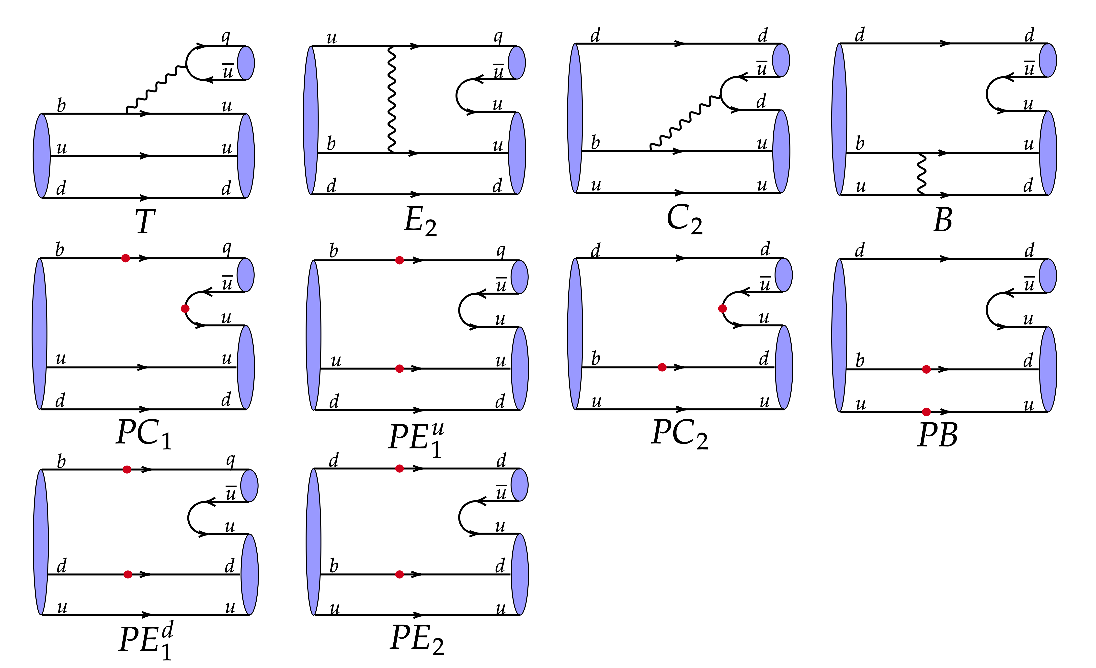
Figure 1: Topological diagrams contributing to the $\Lambda_{b}\to ph$ decays.

The topologies $C_{2}$, $E_{2}$ and $B$, existing in baryon decays, have no counterparts in meson decays.

There are six types of penguin diagrams Han:2024kgz:

• $PC_{1}$, $PC_{2}$, $PE_{1}^{u}$ and $PB$, whose quark flows are related to those of the tree diagrams $T$, $C_{2}$, $E_{2}$ and $B$, respectively, by the Feriz transformation. The $PC_{1}$ topology can be further classified into the factorizable piece $PC_{1}^{f}$ and the non-factorizable piece $PC_{1}^{nf}$;

• $PE_{1}^{d}$ and $PE_{2}$, which are related to each other through the Feriz transformation without the corresponding tree diagrams.

The $T^{f}$ diagram dominates the tree contributions to the $\Lambda_{b}\to ph$ decays as a consequence of the color transparency mechanism, and can be well estimated by the factorization hypothesis. All the other tree topologies give nonfactorizable contributions. Following the power counting rules in the SCET, we attain the hierarchy among the various tree topologies Leibovich:2003tw

$$\frac{|C_{2}|}{|T|}\sim\frac{|E_{2}|}{|T|}\sim\frac{|B|}{|T|}\sim\mathcal{O}\left(\frac{\Lambda_{\rm QCD}}{m_{b}}\right)^{2},$$ (5)

with the QCD scale $\Lambda_{\rm QCD}$.

II.3 Kinematics

We adopt the light-cone coordinates for assigning the kinematic variables of the $\Lambda_{b}\to ph$ decays. The initial $\Lambda_{b}$ baryon momentum $p_{\Lambda_{b}}$, the proton momentum $p_{p}$ and the meson momentum $q$ are chosen, in the rest frame of the $\Lambda_{b}$ baryon, as

$$\begin{split}p_{\Lambda_{b}}=&\frac{m_{\Lambda_{b}}}{\sqrt{2}}(1,1,\bm{0}_{T}),\\ p_{p}=&\frac{m_{\Lambda_{b}}}{\sqrt{2}}(\eta^{+},\eta^{-},\bm{0}_{T}),\\ q=&p_{\Lambda_{b}}-p_{p}=\frac{m_{\Lambda_{b}}}{\sqrt{2}}(1-\eta^{+},1-\eta^{-},\bm{0}_{T}),\end{split}$$ (6)

where the variables

$$\eta^{\pm}=\left[m_{\Lambda_{b}}^{2}-m_{h}^{2}+m_{p}^{2}\pm\sqrt{(m_{\Lambda_{b}}^{2}-m_{h}^{2}+m_{p}^{2})^{2}-4m_{\Lambda_{b}}^{2}m_{p}^{2}}\right]/(2m_{\Lambda_{b}}^{2}),$$ (7)

are determined by the momentum conservation with the $\Lambda_{b}$ baryon (proton, meson) mass $m_{\Lambda_{b}}$ ($m_{p}$, $m_{h}$). The longitudinal and transverse polarization vectors of a spin-1 final-state meson,

$$\epsilon_{L}=\frac{m_{h}}{\sqrt{2}m_{\Lambda_{b}}}(\eta^{+}-1,1-\eta^{-},\bm{0}_{T}),\quad\epsilon_{T}=(0,0,\bm{1}_{T}),$$ (8)

are fixed by the normalization and orthogonality conditions, which respect $\epsilon_{L}^{2}=-1$ and $\epsilon_{L}\cdot q=0$.

The valence quark momenta in the three involved hadrons are parameterized as

$$k_{1}= (\frac{m_{\Lambda_{b}}}{\sqrt{2}},\frac{m_{\Lambda_{b}}}{\sqrt{2}}x_{1},\bm{k}_{1T}), \quad k_{2}= (0,\frac{m_{\Lambda_{b}}}{\sqrt{2}}x_{2},\bm{k}_{2T}), \quad k_{3}= (0,\frac{m_{\Lambda_{b}}}{\sqrt{2}}x_{3},\bm{k}_{3T}),$$

$$k_{1}^{\prime}= (\frac{m_{\Lambda_{b}}}{\sqrt{2}}\eta^{+}x_{1}^{\prime},0,\bm{k}_{1T}^{\prime}), k_{2}^{\prime}= (\frac{m_{\Lambda_{b}}}{\sqrt{2}}\eta^{+}x_{2}^{\prime},0,\bm{k}_{2T}^{\prime}), k_{3}^{\prime}= (\frac{m_{\Lambda_{b}}}{\sqrt{2}}\eta^{+}x_{3}^{\prime},0,\bm{k}_{3T}^{\prime}),$$

$$q_{1}= (0,\frac{m_{\Lambda_{b}}}{\sqrt{2}}y(1-\eta^{-}),\bm{q}_{T}), q_{2}= (0,\frac{m_{\Lambda_{b}}}{\sqrt{2}}(1-y)(1-\eta^{-}),-\bm{q}_{T}),$$ (9)

where $k_{1}$ is the $b$ quark momentum, and the other momenta are designated in the Feynman diagrams in Appendix. B. The momentum fractions $x_{1,2,3}^{(\prime)}$ and the transverse momenta $\bm{k}_{1T,2T,3T}^{(\prime)}$ obey

$$\sum_{i=1}^{3}x_{i}^{(\prime)}=1,\qquad\sum_{i=1}^{3}\bm{k}_{iT}^{(\prime)}=0,$$ (10)

respectively. We stress that the quark momenta in the $\Lambda_{b}$ baryon should be parametrized as

$$k_{1}=(\frac{m_{\Lambda_{b}}}{\sqrt{2}}(1-x_{3}),\frac{m_{\Lambda_{b}}}{\sqrt{2}}(1-x_{2}),\bm{k}_{1T}),\quad k_{2}=(0,\frac{m_{\Lambda_{b}}}{\sqrt{2}}x_{2},\bm{k}_{2T}),\quad k_{3}=(\frac{m_{\Lambda_{b}}}{\sqrt{2}}x_{3},0,\bm{k}_{3T}),$$ (11)

to maintain the virtuality of hard gluons as evaluating the topologies $C_{2}$, $B$, $PC_{2}$ and $PB$. This special kinematic assignment is allowed in view that light quarks in a $\Lambda_{b}$ baryon are soft, and their momenta can point to different directions in principle.

II.4 Distribution amplitudes

The $\Lambda_{b}$ baryon DAs are defined by the matrix elements of nonlocal operators sandwiched between the vacuum and the $\Lambda_{b}$ baryon state. The general Lorentz structures of these matrix elements can be found in Ball:2008fw; Bell:2013tfa; Wang:2015ndk; Ali:2012zza,

$$\begin{split}(Y_{\Lambda_{b}})_{\alpha\beta\gamma}(x_{i},\mu)&\equiv\frac{1}{2\sqrt{2}N_{c}}\int\prod_{l=2}^{3}\frac{dz_{l}^{-}d\bm{z}_{l}}{(2\pi)^{3}}e^{ik_{l}\cdot z_{l}}\epsilon^{ijk}\langle 0|T[b_{\alpha}^{i}(0)u_{\beta}^{j}(z_{2})d_{\gamma}^{k}(z_{3})]|\Lambda_{b}\rangle\\ &=\frac{1}{8\sqrt{2}N_{c}}\Big{\{}f_{\Lambda_{b}}^{(1)}(\mu)[M_{1}(x_{2},x_{3})\gamma_{5}C^{T}]_{\gamma\beta}+f_{\Lambda_{b}}^{(2)}(\mu)[M_{2}(x_{2},x_{3})\gamma_{5}C^{T}]_{\gamma\beta}\Big{\}}[u_{\Lambda_{b}}]_{\alpha},\end{split}$$ (12)

where $N_{c}$ is the number of colors, $i^{\prime},j^{\prime},k^{\prime}$ are the color indices, $\alpha,\beta,\gamma$ are the Dirac indices, the normalization constants $f_{\Lambda_{b}}^{(1)}\approx f_{\Lambda_{b}}^{(2)}\equiv f_{\Lambda_{b}}=0.022\pm 0.001$ GeV${}^{3}$ are quoted from the leading-order sum-rule result Groote:1997yr, $C$ stands fors the charge conjugation matrix, and $u_{\Lambda_{b}}$ is the $\Lambda_{b}$ baryon spinor. The DAs in Eq. (12) are decomposed into

$$\begin{split}M_{1}(x_{2},x_{3})=&\frac{\not{\bar{n}}\not{n}}{4}\psi_{3}^{+-}(x_{2},x_{3})+\frac{\not{n}\not{\bar{n}}}{4}\psi_{3}^{-+}(x_{2},x_{3}),\\ M_{2}(x_{2},x_{3})=&\frac{\not{n}}{\sqrt{2}}\psi_{2}(x_{2},x_{3})+\frac{\not{\bar{n}}}{\sqrt{2}}\psi_{4}(x_{2},x_{3}),\end{split}$$ (13)

with the light-like vectors $n=(1,0,\bm{0}_{T})$ and $\bar{n}=(0,1,\bm{0}_{T})$. The models with the exponential ansatz Bell:2013tfa are employed

$$\begin{split}\psi_{2}(x_{2},x_{3})=&\frac{x_{2}x_{3}}{\omega_{0}^{4}}m^{4}_{\Lambda_{b}}e^{-(x_{2}+x_{3})m_{\Lambda_{b}}/\omega_{0}},\\ \psi_{3}^{+-}(x_{2},x_{3})=&\frac{2x_{2}}{\omega_{0}^{3}}m^{3}_{\Lambda_{b}}e^{-(x_{2}+x_{3})m_{\Lambda_{b}}/\omega_{0}},\\ \psi_{3}^{-+}(x_{2},x_{3})=&\frac{2x_{3}}{\omega_{0}^{3}}m^{3}_{\Lambda_{b}}e^{-(x_{2}+x_{3})m_{\Lambda_{b}}/\omega_{0}},\\ \psi_{4}(x_{2},x_{3})=&\frac{1}{\omega_{0}^{2}}m_{\Lambda_{b}}^{2}e^{-(x_{2}+x_{3})m_{\Lambda_{b}}/\omega_{0}},\end{split}$$ (14)

where the parameter $\omega_{0}$, with the typical value lower than $1$ GeV, measures the average energy of the two light quarks in a $\Lambda_{b}$ baryon. We extract $\omega_{0}$ from the LHCb data for the $\Lambda_{b}\to p\mu\bar{\nu}_{\mu}$ and $\Lambda_{b}\to pD_{s}^{-}$ branching ratios, $Br(\Lambda_{b}\to p\mu\bar{\nu}_{\mu})=(4.1\pm 1.0)\times 10^{-4}$ and $Br(\Lambda_{b}\to pD_{s}^{-})=(12.5\pm 1.3)\times 10^{-6}$. The former for a semileptonic mode depends on the $\Lambda_{b}\to p$ transition form factors, and the latter involves only the $T$ topology. The comparison between the data and our predictions for various $\omega_{0}$ sets the conservative range $\omega_{0}=0.7\pm 0.1$ GeV as exhibited in Fig. 2, which is higher than the one chosen in light-cone sum rules Wang:2015ndk; Huang:2022lfr. The common extraction $\omega_{0}\approx 0.7$ GeV from the two disparate pieces of data supports the consistency of our framework.

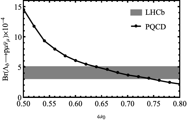
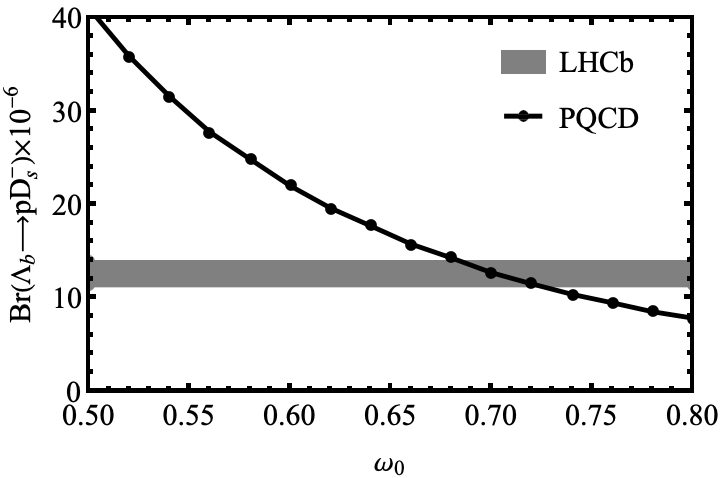
Figure 2: Dependencies of $Br(\Lambda_{b}\to p\mu\bar{\nu}_{\mu})$ (left) and $Br(\Lambda_{b}\to pD_{s}^{-})$ (right) on $\omega_{0}$.

The final-state proton DAs up to twist 6 have been defined in Ref. Braun:2000kw through the corresponding momentum-space projector

$$\begin{split}(\overline{Y}_{P})_{\alpha\beta\gamma}&(x_{i}^{\prime},\mu)\equiv\frac{1}{2\sqrt{2}N_{c}}\int\prod_{l=2}^{3}\frac{dz_{l}^{-}d\bm{z}_{l}}{(2\pi)^{3}}e^{ik^{\prime}_{l}\cdot z_{l}}\epsilon^{i^{\prime}j^{\prime}k^{\prime}}\langle p(p^{\prime})|T[\bar{u}_{\alpha}^{i^{\prime}}(0)\bar{u}_{\beta}^{j^{\prime}}(z_{2})\bar{d}_{\gamma}^{k^{\prime}}(z_{3})]|0\rangle\\ =&\frac{-1}{8\sqrt{2}N_{c}}\Big{\{}S_{1}m_{p}C_{\beta\alpha}(\bar{N}^{+}\gamma_{5})_{\gamma}+S_{2}m_{p}C_{\beta\alpha}(\bar{N}^{-}\gamma_{5})_{\gamma}+P_{1}m_{p}(C\gamma_{5})_{\beta\alpha}\bar{N}^{+}_{\gamma}\\ &+P_{2}m_{p}(C\gamma_{5})_{\beta\alpha}\bar{N}^{-}_{\gamma}+V_{1}(C\not{P})_{\beta\alpha}(\bar{N}^{+}\gamma_{5})_{\gamma}+V_{2}(C\not{P})_{\beta\alpha}(\bar{N}^{-}\gamma_{5})_{\gamma}\\ &+V_{3}\frac{m_{p}}{2}(C\gamma_{\perp})_{\beta\alpha}(\bar{N}^{+}\gamma_{5}\gamma^{\perp})_{\gamma}+V_{4}\frac{m_{p}}{2}(C\gamma_{\perp})_{\beta\alpha}(\bar{N}^{-}\gamma_{5}\gamma^{\perp})_{\gamma}+V_{5}\frac{m_{p}^{2}}{2Pz}(C\not{z})_{\beta\alpha}(\bar{N}^{+}\gamma_{5})_{\gamma}\\ &+V_{6}\frac{m_{p}^{2}}{2Pz}(C\not{z})_{\beta\alpha}(\bar{N}^{-}\gamma_{5})_{\gamma}+A_{1}(C\gamma_{5}\not{P})_{\beta\alpha}(\bar{N}^{+})_{\gamma}+A_{2}(C\gamma_{5}\not{P})_{\beta\alpha}(\bar{N}^{-})_{\gamma}\\ &+A_{3}\frac{m_{p}}{2}(C\gamma_{5}\gamma_{\perp})_{\beta\alpha}(\bar{N}^{+}\gamma^{\perp})_{\gamma}+A_{4}\frac{m_{p}}{2}(C\gamma_{5}\gamma_{\perp})_{\beta\alpha}(\bar{N}^{-}\gamma^{\perp})_{\gamma}+A_{5}\frac{m_{p}^{2}}{2Pz}(C\gamma_{5}\not{z})_{\beta\alpha}(\bar{N}^{+})_{\gamma}\\ &+A_{6}\frac{m_{p}^{2}}{2Pz}(C\gamma_{5}\not{z})_{\beta\alpha}(\bar{N}^{-})_{\gamma}-T_{1}(iC\sigma_{\perp P})_{\beta\alpha}(\bar{N}^{+}\gamma_{5}\gamma^{\perp})_{\gamma}-T_{2}(iC\sigma_{\perp P})_{\beta\alpha}(\bar{N}^{-}\gamma_{5}\gamma^{\perp})_{\gamma}\\ &-T_{3}\frac{m_{p}}{Pz}(iC\sigma_{Pz})_{\beta\alpha}(\bar{N}^{+}\gamma_{5})_{\gamma}-T_{4}\frac{m_{p}}{Pz}(iC\sigma_{zP})_{\beta\alpha}(\bar{N}^{-}\gamma_{5})_{\gamma}-T_{5}\frac{m_{p}^{2}}{2Pz}(iC\sigma_{\perp z})_{\beta\alpha}(\bar{N}^{+}\gamma_{5}\gamma^{\perp})_{\gamma}\\ &-T_{6}\frac{m_{p}^{2}}{2Pz}(iC\sigma_{\perp z})_{\beta\alpha}(\bar{N}^{-}\gamma_{5}\gamma^{\perp})_{\gamma}+T_{7}\frac{m_{p}}{2}(C\sigma_{\perp\perp^{\prime}})_{\beta\alpha}(\bar{N}^{+}\gamma_{5}\sigma^{\perp\perp^{\prime}})_{\gamma}\\ &+T_{8}\frac{m_{p}}{2}(C\sigma_{\perp\perp^{\prime}})_{\beta\alpha}(\bar{N}^{-}\gamma_{5}\sigma^{\perp\perp^{\prime}})_{\gamma}\Big{\}},\end{split}$$ (15)

with the color indices $i^{\prime},j^{\prime},k^{\prime}$. The light-like vector $P$ is written, in terms of the proton momentum $p_{p}$ and the light-like vector $z$, as

$$P^{\mu}=p_{p}^{\mu}-\frac{1}{2}z^{\mu}\frac{m_{p}^{2}}{Pz},$$ (16)

with $Pz\sim p_{p}z\sim 1$, and the shorthand notation $\sigma_{Pz}=\sigma^{\nu\mu}P_{\nu}z_{\mu}$ has been used. Furthermore, $\bar{N}^{+}=\bar{N}\not{z}\not{P}/(2Pz)$ and $\bar{N}^{-}=\bar{N}\not{P}\not{z}/(2Pz)$ are introduced to represent the ”large” and ”small” components of the proton spinor $\bar{N}$, respectively. The symbol $\perp$ labels the projection perpendicular to $z$ or $P$, and the contraction $\gamma_{\perp}\gamma^{\perp}=\gamma^{\mu}g_{\mu\nu}^{\perp}\gamma^{\nu}$ is perceived with $g_{\mu\nu}^{\perp}=g_{\mu\nu}-(P_{\mu}z_{\nu}+z_{\mu}P_{\nu})/Pz$. The functions $V_{i}$, $A_{i}$, $T_{i}$, $S_{i}$ and $P_{i}$ are classified according to their twists:

• Twist-3 DAs
  

  $$V_{1}(x_{i}^{\prime})= 120x_{1}^{\prime}x_{2}^{\prime}x_{3}^{\prime}[\phi_{3}^{0}+\phi_{3}^{+}(1-3x_{3}^{\prime})],$$

  $$A_{1}(x_{i}^{\prime})= 120x_{1}^{\prime}x_{2}^{\prime}x_{3}^{\prime}(x_{2}^{\prime}-x_{1}^{\prime})\phi_{3}^{-},$$

  $$T_{1}(x_{i}^{\prime})= 120x_{1}^{\prime}x_{2}^{\prime}x_{3}^{\prime}[\phi_{3}^{0}+\frac{1}{2}(\phi_{3}^{-}-\phi_{3}^{+})(1-3x_{3}^{\prime})];$$ (17)

• Twist-4 DAs
  

  $$V_{2}(x_{i}^{\prime})= 24x_{1}^{\prime}x_{2}^{\prime}[\phi_{4}^{0}+\phi_{4}^{+}(1-5x_{3}^{\prime})],$$

  $$V_{3}(x_{i}^{\prime})= 12x_{3}^{\prime}[\psi_{4}^{0}(1-x_{3}^{\prime})+\psi_{4}^{-}(x_{1}^{\prime 2}+x_{2}^{\prime 2}-x_{3}^{\prime}(1-x_{3}^{\prime}))+\psi_{4}^{+}(1-x_{3}^{\prime}-10x_{1}^{\prime}x_{2}^{\prime})],$$

  $$A_{2}(x_{i}^{\prime})= 24x_{1}^{\prime}x_{2}^{\prime}(x_{2}^{\prime}-x_{1}^{\prime})\phi_{4}^{-},$$

  $$A_{3}(x_{i}^{\prime})= 12x_{3}^{\prime}(x_{2}^{\prime}-x_{1}^{\prime})[(\psi_{4}^{0}+\psi_{4}^{+})+\psi_{4}^{-}(1-2x_{3}^{\prime})],$$

  $$T_{2}(x_{i}^{\prime})= 24x_{1}^{\prime}x_{2}^{\prime}[\xi_{4}^{0}+\xi_{4}^{+}(1-5x_{3}^{\prime})],$$

  $$T_{3}(x_{i}^{\prime})= 6x_{3}^{\prime}[(\xi_{4}^{0}+\phi_{4}^{0}+\psi_{4}^{0})(1-x_{3}^{\prime})+(\xi_{4}^{-}+\phi_{4}^{-}-\psi_{4}^{-})(x_{1}^{\prime 2}+x_{2}^{\prime 2}-x_{3}^{\prime}(1-x_{3}^{\prime}))$$

  $$+(\xi_{4}^{+}+\phi_{4}^{+}+\psi_{4}^{+})(1-x_{3}^{\prime}-10x_{1}^{\prime}x_{2}^{\prime})],$$

  $$T_{7}(x_{i}^{\prime})= 6x_{3}^{\prime}[(-\xi_{4}^{0}+\phi_{4}^{0}+\psi_{4}^{0})(1-x_{3}^{\prime})+(-\xi_{4}^{-}+\phi_{4}^{-}-\psi_{4}^{-})(x_{1}^{\prime 2}+x_{2}^{\prime 2}-x_{3}^{\prime}(1-x_{3}^{\prime}))$$

  $$+(-\xi_{4}^{+}+\phi_{4}^{+}+\psi_{4}^{+})(1-x_{3}^{\prime}-10x_{1}^{\prime}x_{2}^{\prime})],$$

  $$S_{1}(x_{i}^{\prime})= 6x_{3}^{\prime}(x_{2}^{\prime}-x_{1}^{\prime})[(\xi_{4}^{0}+\phi_{4}^{0}+\psi_{4}^{0}+\xi_{4}^{+}+\phi_{4}^{+}+\psi_{4}^{+})+(\xi_{4}^{-}+\phi_{4}^{-}-\psi_{4}^{-})(1-2x_{3}^{\prime})],$$

  $$P_{1}(x_{i}^{\prime})= 6x_{3}^{\prime}(x_{2}^{\prime}-x_{1}^{\prime})[(\xi_{4}^{0}-\phi_{4}^{0}-\psi_{4}^{0}+\xi_{4}^{+}-\phi_{4}^{+}-\psi_{4}^{+})+(\xi_{4}^{-}-\phi_{4}^{-}+\psi_{4}^{-})(1-2x_{3}^{\prime})];$$ (18)

• Twist-5 DAs
  

  $$V_{4}(x_{i}^{\prime})= 3[\psi_{5}^{0}(1-x_{3}^{\prime})+\psi_{5}^{-}(2x_{1}^{\prime}x_{2}^{\prime}-x_{3}^{\prime}(1-x_{3}^{\prime}))+\psi_{5}^{+}(1-x_{3}^{\prime}-2(x_{1}^{\prime 2}+x_{2}^{\prime 2}))],$$

  $$V_{5}(x_{i}^{\prime})= 6x_{3}^{\prime}[\phi_{5}^{0}+\phi_{5}^{+}(1-2x_{3}^{\prime})],$$

  $$A_{4}(x_{i}^{\prime})= 3(x_{2}^{\prime}-x_{1}^{\prime})[-\psi_{5}^{0}+\psi_{5}^{-}x_{3}^{\prime}+\psi_{5}^{+}(1-2x_{3}^{\prime})],$$

  $$A_{5}(x_{i}^{\prime})= 6x_{3}^{\prime}(x_{2}^{\prime}-x_{1}^{\prime})\phi_{5}^{-},$$

  $$T_{4}(x_{i}^{\prime})= \frac{3}{2}[(\xi_{5}^{0}+\psi_{5}^{0}+\phi_{5}^{0})(1-x_{3}^{\prime})+(\xi_{5}^{-}+\phi_{5}^{-}-\psi_{5}^{-})(2x_{1}^{\prime}x_{2}^{\prime}-x_{3}^{\prime}(1-x_{3}^{\prime}))$$

  $$+(\xi_{5}^{+}+\phi_{5}^{+}+\psi_{5}^{+})(1-x_{3}^{\prime}-2(x_{1}^{\prime 2}+x_{2}^{\prime 2}))],$$

  $$T_{5}(x_{i}^{\prime})= 6x_{3}^{\prime}[\xi_{5}^{0}+\xi_{5}^{+}(1-2x_{3}^{\prime})],$$

  $$T_{8}(x_{i}^{\prime})= \frac{3}{2}[(\psi_{5}^{0}+\phi_{5}^{0}-\xi_{5}^{0})(1-x_{3}^{\prime})+(\phi_{5}^{-}-\phi_{5}^{-}-\xi_{5}^{-})(2x_{1}^{\prime}x_{2}^{\prime}-x_{3}^{\prime}(1-x_{3}^{\prime}))$$ (19)

  $$+(\phi_{5}^{+}+\phi_{5}^{+}-\xi_{5}^{+})(1-x_{3}^{\prime}-2(x_{1}^{\prime 2}+x_{2}^{\prime 2}))],$$

  $$S_{2}(x_{i}^{\prime})= \frac{3}{2}(x_{2}^{\prime}-x_{1}^{\prime})[-(\psi_{5}^{0}+\phi_{5}^{0}+\xi_{5}^{0})+(\xi_{5}^{-}+\phi_{5}^{-}-\psi_{5}^{0})x_{3}^{\prime}+(\xi_{5}^{+}+\phi_{5}^{+}+\psi_{5}^{0})(1-2x_{3}^{\prime})],$$

  $$P_{2}(x_{i}^{\prime})= \frac{3}{2}(x_{2}^{\prime}-x_{1}^{\prime})[(\psi_{5}^{0}+\phi_{5}^{0}-\xi_{5}^{0})+(\xi_{5}^{-}-\phi_{5}^{-}+\psi_{5}^{0})x_{3}^{\prime}+(\xi_{5}^{+}-\phi_{5}^{+}-\psi_{5}^{0})(1-2x_{3}^{\prime})];$$ (20)

• Twist-6 DAs
  

  $$V_{6}(x_{i}^{\prime})= 2[\phi_{6}^{0}+\phi_{6}^{+}(1-3x_{3}^{\prime})],$$

  $$A_{6}(x_{i}^{\prime})= 2(x_{2}^{\prime}-x_{1}^{\prime})\phi_{6}^{-},$$

  $$T_{6}(x_{i}^{\prime})= 2[\phi_{6}^{0}+\frac{1}{2}(\phi_{6}^{-}-\phi_{6}^{+})(1-3x_{3}^{\prime})].$$ (21)

The values of $\phi_{i}^{\pm,0},\psi_{i}^{\pm,0}$ and $\xi_{i}^{\pm,0}$ are connected to the eight independent parameters $f_{N}$, $\lambda_{1}$, $\lambda_{2}$, $V_{1}^{d}$, $A_{1}^{u}$, $f_{1}^{d}$, $f_{2}^{d}$ and $f_{1}^{u}$ Braun:2000kw,

$$\phi_{3}^{0} =\phi_{6}^{0}=f_{N},\qquad\phi_{4}^{0}=\phi_{5}^{0}=\frac{1}{2}(\lambda_{1}+f_{N}),$$

$$\xi_{4}^{0} =\xi_{5}^{0}=\frac{1}{6}\lambda_{2},\qquad\psi_{4}^{0}=\psi_{5}^{0}=\frac{1}{2}(f_{N}-\lambda_{1}),$$

$$\phi_{4}^{-} =\frac{5}{4}\left(\lambda_{1}(1-2f_{1}^{d}-4f_{1}^{u})+f_{N}(2A_{1}^{u}-1)\right),$$

$$\phi_{4}^{+} =\frac{1}{4}\left(\lambda_{1}(3-10f_{1}^{d})-f_{N}(10V_{1}^{d}-3)\right),$$

$$\psi_{4}^{-} =-\frac{5}{4}\left(\lambda_{1}(2-7f_{1}^{d}+f_{1}^{u})+f_{N}(A_{1}^{u}+3V_{1}^{d}-2)\right),$$

$$\psi_{4}^{+} =-\frac{1}{4}\left(\lambda_{1}(-2+5f_{1}^{d}+5f_{1}^{u})+f_{N}(2+5A_{1}^{u}-5V_{1}^{d})\right),$$

$$\xi_{4}^{-} =\frac{5}{16}\lambda_{2}(4-15f_{2}^{d}),\qquad\xi_{4}^{+}=\frac{1}{16}\lambda_{2}(4-15f_{2}^{d}),$$

$$\phi_{5}^{-} =\frac{5}{3}\left(\lambda_{1}(f_{1}^{d}-f_{1}^{u})+f_{N}(2A_{1}^{u}-1)\right),$$

$$\phi_{5}^{+} =-\frac{5}{6}\left(\lambda_{1}(4f_{1}^{d}-1)+f_{N}(3+4V_{1}^{d})\right),$$

$$\psi_{5}^{-} =\frac{5}{3}\left(\lambda_{1}(f_{1}^{d}-f_{1}^{u})+f_{N}(2-A_{1}^{u}-3V_{1}^{d})\right),$$

$$\psi_{5}^{+} =-\frac{5}{6}\left(\lambda_{1}(-1+2f_{1}^{d}+2f_{1}^{u})+f_{N}(5+2A_{1}^{u}-2V_{1}^{d})\right),$$

$$\xi_{5}^{-} =-\frac{5}{4}\lambda_{2}f_{2}^{d},\qquad\xi_{5}^{+}=\frac{5}{36}\lambda_{2}(2-9f_{2}^{d}),$$

$$\phi_{6}^{-} =\frac{1}{2}\left(\lambda_{1}(1-4f_{1}^{d}-2f_{1}^{u})+f_{N}(1+4A_{1}^{u})\right),$$

$$\phi_{6}^{+} =-\frac{1}{2}\left(\lambda_{1}(1-2f_{1}^{d})+f_{N}(4V_{1}^{d}-1)\right).$$ (22)

These parameters have been derived in QCD sum rules (QCDSR) Braun:2000kw; Braun:2006hz and lattice QCD (LQCD) RQCD:2019hps, whose results are summarized in Table 2. They come with large uncertainties, reflecting our limited knowledge on baryon DAs. We will take the set of parameters from QCDSR Braun:2006hz for the numerical investigations.

Table 2: The eight independent parameters for Eq. (22) at the scale $1$ GeV from QCDSR and LQCD.

	$f_{N}({\rm GeV}^{2})$	$\lambda_{1}({\rm GeV}^{2})$	$\lambda_{2}({\rm GeV}^{2})$	$V_{1}^{d}$
QCDSR(2001)Braun:2000kw	$(5.3\pm 0.5)\times 10^{-3}$	$-(2.7\pm 0.9)\times 10^{-2}$	$(5.1\pm 1.9)\times 10^{-2}$	$0.23\pm 0.03$
QCDSR(2006)Braun:2006hz	$(5.0\pm 0.5)\times 10^{-3}$	$-(2.7\pm 0.9)\times 10^{-2}$	$(5.4\pm 1.9)\times 10^{-2}$	$0.23\pm 0.03$
LQCD(2019)RQCD:2019hps	$(3.54\pm 0.06)\times 10^{-3}$	$-(4.49\pm 0.42)\times 10^{-2}$	$(9.34\pm 0.48)\times 10^{-2}$	$0.19\pm 0.22$
	$A_{1}^{u}$	$f_{1}^{d}$	$f_{2}^{d}$	$f_{1}^{u}$
QCDSR(2001)Braun:2000kw	$0.38\pm 0.15$	$0.6\pm 0.2$	$0.15\pm 0.06$	$0.22\pm 0.15$
QCDSR(2006)Braun:2006hz	$0.38\pm 0.15$	$0.4\pm 0.05$	$0.22\pm 0.05$	$0.07\pm 0.05$
LQCD(2019)RQCD:2019hps	$0.30\pm 0.32$	…	…	…

The DAs for a pseudoscalar meson are expanded, up to twist 3, as Chernyak:1983ej; Braun:1988qv; Braun:1989iv; Kurimoto:2001zj

$$\begin{split}\Phi_{\pi(K)}(q,y)=&\int d^{4}ze^{-iyq\cdot z}\langle\pi(K)(q)|\bar{q}_{\beta}(z)u_{\alpha}(0)|0\rangle\\ =&\frac{i}{\sqrt{2N_{C}}}\left[\gamma_{5}\not{q}\phi_{\pi(K)}^{A}(y)+m_{0}^{\pi(K)}\gamma_{5}\phi_{\pi(K)}^{P}(y)+m_{0}^{\pi(K)}\gamma_{5}(\not{v}\not{n}-1)\phi_{\pi(K)}^{T}(y)\right]_{\alpha\beta},\end{split}$$ (23)

where $m_{0}^{\pi(K)}=m_{\pi(K)}^{2}/(m_{u}+m_{d(s)})$, $m_{u}$ ($m_{d}$, $m_{s}$) being the $u$ ($d$, $s$) quark mass, is the chiral scale associated with the pseudoscalar meson, and the momentum fraction $y$ is carried by the quark in the meson. The DAs are parameterized as Ball:2004ye; Ball:2006wn,

$$\begin{split}\phi^{A}_{\pi(K)}(y)=&\frac{f_{\pi(K)}}{2\sqrt{2N_{c}}}6y(1-y)\left[1+a_{1}^{\pi(K)}C_{1}^{3/2}(2y-1)+a_{2}^{\pi(K)}C_{2}^{3/2}(2y-1)+a_{4}^{\pi(K)}C_{4}^{3/2}(2y-1)\right],\\ \phi^{P}_{\pi(K)}(y)=&\frac{f_{\pi(K)}}{2\sqrt{2N_{c}}}\bigg{[}1+\left(0.45-\frac{5}{2}\rho_{\pi(K)}^{2}\right)C_{2}^{1/2}(2y-1)\\ &-3\left(-0.045+\frac{9}{20}\rho_{\pi(K)}^{2}(1+6a_{2}^{\pi(K)})\right)C_{4}^{1/2}(2y-1)\bigg{]},\\ \phi^{T}_{\pi(K)}(y)=&\frac{f_{\pi(K)}}{2\sqrt{2N_{c}}}(1-2y)\left[1+6\left(0.0975-\frac{7}{20}\rho_{\pi(K)}^{2}-\frac{3}{5}\rho_{\pi(K)}^{2}a_{2}^{\pi(K)}\right)(1-10y+10y^{2})\right],\end{split}$$ (24)

with the decay constant $f_{\pi(K)}=0.13$ (0.16) GeV, the Gegenbauer polynomials $C_{n}^{\nu}$, $\nu=1/2,3/2$ and $n=1,2,4$, and the other parameters Ball:2004ye; Ball:2006wn,

$$\begin{split}a_{1}^{\pi}=0,&\qquad a_{1}^{K}=0.06,\\ a_{2}^{\pi}=0.25\pm 0.15,&\qquad a_{2}^{K}=0.25\pm 0.15,\\ a_{4}^{\pi}=-0.015,&\qquad a_{4}^{K}=0,\\ m_{\pi}=0.14\;\text{GeV},&\qquad m_{K}=0.494\;\text{GeV},\\ m_{0}^{\pi}=(1.4\pm 0.1)\;\text{GeV},&\qquad m_{0}^{K}=(1.6\pm 0.1)\;\text{GeV},\\ \rho_{\pi}=\frac{m_{\pi}}{m_{0}^{\pi}},&\qquad\rho_{K}=\frac{m_{K}}{m_{0}^{K}}.\end{split}$$ (25)

The vector meson DAs are defined by Li:2009tx

$$\begin{split}\Phi_{V}^{L}(q,\epsilon_{L}^{\ast},y)=&\int d^{4}ze^{-iyq\cdot z}\langle V(q,\epsilon_{L}^{\ast})|\bar{q}_{\beta}(z)u_{\alpha}(0)|0\rangle\\ =&\frac{-1}{\sqrt{2N_{c}}}\left[m_{V}\not{\epsilon}_{L}^{\ast}\phi_{V}(y)+\not{\epsilon}_{L}^{\ast}\not{q}\phi_{V}^{t}(y)+m_{V}\phi_{V}^{s}(y)\right]_{\alpha\beta},\end{split}$$ (26)

$$\begin{split}\Phi_{V}^{T}(q,\epsilon_{T}^{\ast},y)=&\int d^{4}ze^{-iyq\cdot z}\langle V(q,\epsilon_{T}^{\ast})|\bar{q}_{\beta}(z)u_{\alpha}(0)|0\rangle\\ =&\frac{-1}{\sqrt{2N_{c}}}\left[m_{V}\not{\epsilon}_{T}^{\ast}\phi_{V}^{v}(y)+\not{\epsilon}_{T}^{\ast}\not{q}\phi_{V}^{T}(y)+m_{V}i\epsilon_{\mu\nu\rho\sigma}\gamma_{5}\gamma^{\mu}\epsilon_{T}^{\ast\nu}v^{\rho}n^{\sigma}\phi_{V}^{a}(y)\right]_{\alpha\beta},\end{split}$$ (27)

with the vector meson mass $m_{V}$. The twist-2 DAs are also expanded int terms of the Gegenbauer polynomials,

$$\phi_{V}(y)= \frac{3f_{V}}{\sqrt{2N_{c}}}y(1-y)\left[1+a_{1}^{\parallel}C_{1}^{3/2}(2y-1)+a_{2}^{\parallel}C_{2}^{3/2}(2y-1)\right],$$

$$\phi_{V}^{T}(y)= \frac{3f_{V}^{T}}{\sqrt{2N_{c}}}y(1-y)\left[1+a_{1}^{\perp}C_{1}^{3/2}(2y-1)+a_{2}^{\perp}C_{2}^{3/2}(2y-1)\right].$$ (28)

The asymptotic forms are assumed for the twist-3 DAs, Ali:2007ff,

$$\phi_{V}^{t}(y)= \frac{3f_{V}^{T}}{2\sqrt{2N_{c}}}(2y-1)^{2},$$

$$\phi_{V}^{s}(y)= \frac{3f_{V}^{T}}{2\sqrt{2N_{c}}}(1-2y),$$

$$\phi_{V}^{v}(y)= \frac{3f_{V}}{8\sqrt{2N_{c}}}(1+(2y-1)^{2}),$$

$$\phi_{V}^{a}(y)= \frac{3f_{V}}{4\sqrt{2N_{c}}}(1-2y).$$ (29)

The Gegenbauer moments $a_{n}$ in the above expansions have been obtained in QCDSR Braun:2004vf; Ball:2005vx; Ball:2006nr; Ball:2007rt, which, together with the decay constants, are collected in Table 3.

Table 3: Inputs of the decay constants (in MeV) and the Gegenbauer moments for the vector meson DAs.

$f_{\rho}$	$f_{\rho}^{T}$	$f_{K^{\ast}}$	$f_{K^{\ast}}^{T}$
$209\pm 2$	$165\pm 9$	$217\pm 5$	$185\pm 10$
$a_{1\rho}^{\parallel}$	$a_{1\rho}^{\perp}$	$a_{1K^{\ast}}^{\parallel}$	$a_{1K^{\ast}}^{\perp}$
0	0	$0.03\pm 0.02$	$0.04\pm 0.03$
$a_{2\rho}^{\parallel}$	$a_{2\rho}^{\perp}$	$a_{2K^{\ast}}^{\parallel}$	$a_{2K^{\ast}}^{\perp}$
$0.15\pm 0.07$	$0.14\pm 0.06$	$0.11\pm 0.09$	$0.10\pm 0.08$

The DAs for an axial-vector with the quantum number $J^{P}=1^{+}$ are introduced through Li:2009tx,

$$\begin{split}\Phi_{A}^{L}(q,\epsilon_{L}^{\ast},y)=&\int d^{4}ze^{-iyq\cdot z}\langle A(q,\epsilon_{L}^{\ast})|\bar{q}_{\beta}(z)u_{\alpha}(0)|0\rangle\\ =&\frac{-i}{\sqrt{2N_{c}}}\left[m_{A}\gamma_{5}\not{\epsilon}_{L}^{\ast}\phi_{A}(y)+\not{\epsilon}_{L}^{\ast}\not{q}\gamma_{5}\phi_{A}^{t}(y)+m_{A}\gamma_{5}\phi_{A}^{s}(y)\right]_{\alpha\beta},\end{split}$$ (30)

$$\begin{split}\Phi_{A}^{T}(q,\epsilon_{T}^{\ast},y)=&\int d^{4}ze^{-iyq\cdot z}\langle A(q,\epsilon_{T}^{\ast})|\bar{q}_{\beta}(z)u_{\alpha}(0)|0\rangle\\ &\frac{-i}{\sqrt{2N_{c}}}\left[m_{A}\gamma_{5}\not{\epsilon}_{T}^{\ast}\phi_{A}^{v}(y)+\not{\epsilon}_{T}^{\ast}\not{q}\gamma_{5}\phi_{A}^{T}(y)+m_{A}i\epsilon_{\mu\nu\rho\sigma}\gamma^{\mu}\epsilon_{T}^{\ast\nu}v^{\rho}n^{\sigma}\phi_{A}^{a}(y)\right]_{\alpha\beta},\end{split}$$ (31)

with the axial-vector meson mass $m_{A}$. The twist-2 and twist-3 DAs read

$$\phi_{A}(y)= \frac{3f_{A}}{\sqrt{2N_{c}}}y(1-y)\left[a_{0A}^{\parallel}+3a_{1A}^{\parallel}(2y-1)+\frac{3}{2}a_{2A}^{\parallel}(5(2y-1)^{2}-1)\right],$$

$$\phi_{A}^{T}(y)= \frac{3f_{A}}{\sqrt{2N_{c}}}y(1-y)\left[a_{0A}^{\perp}+3a_{1A}^{\perp}(2y-1)+\frac{3}{2}a_{2A}^{\perp}(5(2y-1)^{2}-1)\right],$$ (32)

and

$$\phi_{A}^{t}(y)= \frac{f_{A}}{2\sqrt{2N_{c}}}\left[3a_{0A}^{\perp}(2y-1)^{2}+\frac{3}{2}a_{1A}^{\perp}(2y-1)(3(2y-1)^{2}-1)\right],$$

$$\phi_{A}^{s}(y)= \frac{3f_{A}}{2\sqrt{2N_{c}}}(a_{0A}^{\perp}-a_{1A}^{\perp}-2a_{0A}^{\perp}y+6a_{1A}^{\perp}y-6a_{1A}^{\perp}y^{2}),$$

$$\phi_{A}^{v}(y)= \frac{f_{A}}{2\sqrt{2N_{c}}}\left[\frac{3}{4}a_{0A}^{\parallel}(1+(2y-1)^{2})+\frac{3}{2}a_{1A}^{\parallel}(2y-1)^{3}\right],$$

$$\phi_{A}^{a}(y)= \frac{3f_{A}}{4\sqrt{2N_{c}}}(a_{0A}^{\parallel}-a_{1A}^{\parallel}-2a_{0A}^{\parallel}y+6a_{1A}^{\parallel}y-6a_{1A}^{\parallel}y^{2}),$$ (33)

respectively. The associated decay constants and Gegenbauer moments are listed in Table 4.

Table 4: Same as Table 3 but for the axial-vector meson DAs.

$f_{a_{1}(1260)}$	$a_{0a_{1}(1260)}^{\parallel}$	$a_{1a_{1}(1260)}^{\parallel}$	$a_{2a_{1}(1260)}^{\parallel}$
$238\pm 10$	1	0	$-0.02\pm 0.02$
	$a_{0a_{1}(1260)}^{\perp}$	$a_{1a_{1}(1260)}^{\perp}$	$a_{2a_{1}(1260)}^{\perp}$
	0	$-1.04\pm 0.34$	0
$f_{K_{1A}}$	$a_{0K_{1A}}^{\parallel}$	$a_{1K_{1A}}^{\parallel}$	$a_{2K_{1A}}^{\parallel}$
$250\pm 13$	1	$0.00\pm 0.26$	$-0.05\pm 0.03$
	$a_{0K_{1A}}^{\perp}$	$a_{1K_{1A}}^{\perp}$	$a_{2K_{1A}}^{\perp}$
	$0.08\pm 0.09$	$-1.08\pm 0.48$	$0.02\pm 0.20$
$f_{K_{1B}}$	$a_{0K_{1B}}^{\parallel}$	$a_{1K_{1B}}^{\parallel}$	$a_{2K_{1B}}^{\parallel}$
$190\pm 10$	$0.14\pm 0.15$	$-1.95\pm 0.45$	$0.02\pm 0.10$
	$a_{0K_{1B}}^{\perp}$	$a_{1K_{1B}}^{\perp}$	$a_{2K_{1B}}^{\perp}$
	1	$0.17\pm 0.22$	$-0.02\pm 0.22$

The physical mass eigenstates $K_{1}(1270)$ and $K_{1}(1400)$ are considered to be the mixtures of the $K_{1A}(^{3}P_{1})$ and $K_{1B}(^{1}P_{1})$ states with the mixing angle $\theta_{K_{1}}$:

$$\left(\begin{array}[]{c}|K_{1}(1270)\rangle\\ |K_{1}(1400)\rangle\end{array}\right)=\left(\begin{array}[]{cc}\sin\theta_{K_{1}}&\cos\theta_{K_{1}}\\ \cos\theta_{K_{1}}&-\sin\theta_{K_{1}}\end{array}\right)\left(\begin{array}[]{c}|K_{1A}\rangle\\ |K_{1B}\rangle\end{array}\right),$$ (34)

in which $\theta_{K_{1}}$ is chosen as the typical values $30^{\circ}$ and $60^{\circ}$ suggested in Refs.Cheng:2013cwa; Hatanaka:2008xj; Cheng:2011pb; Shi:2023kiy.

For reader’s reference, we present the explicit expressions for the relevant Gegenbauer polynomials $C_{n}^{\nu}(t)$,

$$\begin{split}C_{1}^{3/2}(t)=&3t,\\ C_{2}^{1/2}(t)=&\frac{1}{2}(3t^{2}-1),\\ C_{2}^{3/2}(t)=&\frac{3}{2}(5t^{2}-1),\\ C_{4}^{1/2}(t)=&\frac{1}{8}(3-30t^{2}+35t^{4}),\\ C_{4}^{3/2}(t)=&\frac{15}{8}(1-14t^{2}+21t^{4}),\end{split}$$ (35)

and the definitions of the meson decay constants,

$$\begin{split}\langle P|(\bar{q}q^{\prime})_{V\mp A}|0\rangle=&\pm if_{P}p_{\mu},\qquad\quad\langle P|(\bar{q}q^{\prime})_{S\mp P}|0\rangle=\pm if_{P}m_{0P},\\ \langle V|(\bar{q}q^{\prime})_{V\mp A}|0\rangle=&f_{V}m_{V}\epsilon_{\mu}^{\ast},\qquad\quad\langle V|(\bar{q}q^{\prime})_{S\mp P}|0\rangle=0,\\ \langle A|(\bar{q}q^{\prime})_{V\mp A}|0\rangle=&\mp if_{A}m_{A}\epsilon_{\mu}^{\ast},\qquad\langle A|(\bar{q}q^{\prime})_{S\mp P}|0\rangle=0.\end{split}$$ (36)

II.5 Numerical integration

The PQCD factorization formulas and the auxiliary functions from Fourier transformation in Appendices A and B are extremely complicated, containing $11\sim 13$ dimensional integrations. Computing high dimensional integrals effectively and making precise predictions for heavy baryon decays thus remain a numerical challenge. Various algorithms have been proposed, among which the VEGAS+ is one of the most widely used in particle physics. The classic VEGAS performs a multidimensional Monte Carlo integration based on adaptive importance sampling, originally developed by G.P. Lepage Lepage:1977sw. It then evolved to the VEGAS+ by incorporating a second strategy known as adaptive stratified sampling Lepage:2020tgj. It is believed that the VEGAS+ is much more efficient for handling integrands with multiple peaks compared to the VEGAS. See Ref. Lepage:2020tgj and references therein for more details of the VEGAS+ algorithm.

When applying the VEGAS+ to the integrations involved in this work, we encounter a subtlety, which can be illustrated by taking the diagram $T(d5)$ in Fig. 15 as an example. This diagram gives a non-factorizable amplitude with the auxiliary function $F_{4}$, The numerical outcomes from the VEGAS+ for the $T(d5)$ contributions after $15$ iterations are plotted in Fig. 3, where the number of samples increases from $10^{4}$ to $10^{8}$. It is observed that the statistical errors in the imaginary parts decrease as $1/\sqrt{N_{ev}}$, consistent with the characteristics of a Monte Carlo algorithm. However, the real parts do not converge, meaning that the VEGAS+ is ineffective for the real parts.

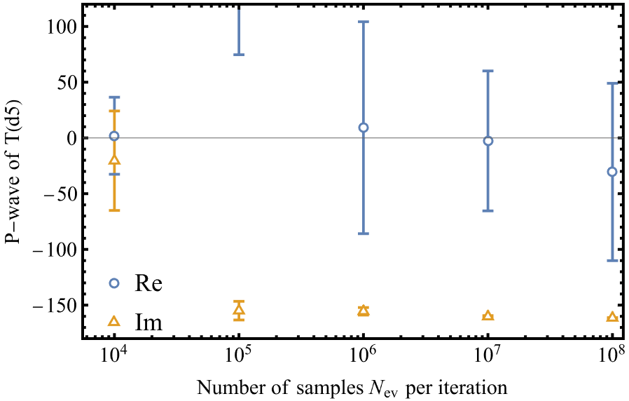
Figure 3: (left) Numerical results of the $T(d5)$ contribution to the $S$-wave from the VEGAS+ after $15$ iterations with increasing numbers of samples; (right) same as the left panel but for the $P$-wave.

We find that the real parts of the diagrams with the auxiliary function $F_{1}$ can be accurately acquired, but those depending on $F_{2,3,4}$ cannot. To elaborate the issue, we introduce the functions $B^{(1)}(x)\equiv K_{0}(\sqrt{x})\Theta(x)+\frac{i\pi}{2}H_{0}^{(1)}(\sqrt{-x})\Theta(-x)$ and $B^{(2)}(x)\equiv K_{1}(\sqrt{x})\Theta(x)-\frac{i\pi}{2}H_{1}^{(1)}(\sqrt{-x})\Theta(-x)$, where the step function $\Theta(x)$ equals $1$ when $x>0$ and $0$ otherwise. The former (latter) corresponds to the Bessel function appearing in $F_{1}$ ($F_{2,3,4}$). As described in Fig. 4, both $B^{(1)}(x)$ and $B^{(2)}(x)$ are singular at $x=0$ with the limits,

$$\begin{split}\displaystyle\lim_{x\to 0^{-}}B^{(1)}(x)&=-\displaystyle\lim_{x\to 0^{-}}\text{log}(\sqrt{-x})+\frac{i\pi}{2},\\ \displaystyle\lim_{x\to 0^{+}}B^{(1)}(x)&=-\displaystyle\lim_{x\to 0^{+}}\text{log}(\sqrt{x}),\\ \displaystyle\lim_{x\to 0^{-}}B^{(2)}(x)&=\displaystyle\lim_{x\to 0^{-}}\frac{-1}{\sqrt{-x}},\\ \displaystyle\lim_{x\to 0^{+}}B^{(2)}(x)&=\displaystyle\lim_{x\to 0^{+}}\frac{1}{\sqrt{x}}.\end{split}$$ (37)

The real part of $B^{(1)}(x)$ behaves like $\text{log}(\sqrt{|x|})$ on both sides of $x=0$, which can be well managed by the VEGAS+. However, the real part of $B^{(2)}(x)$ approaches $\pm\infty$ from the two sides of $x=0$, whose incomplete cancellation causes the numerical instability.

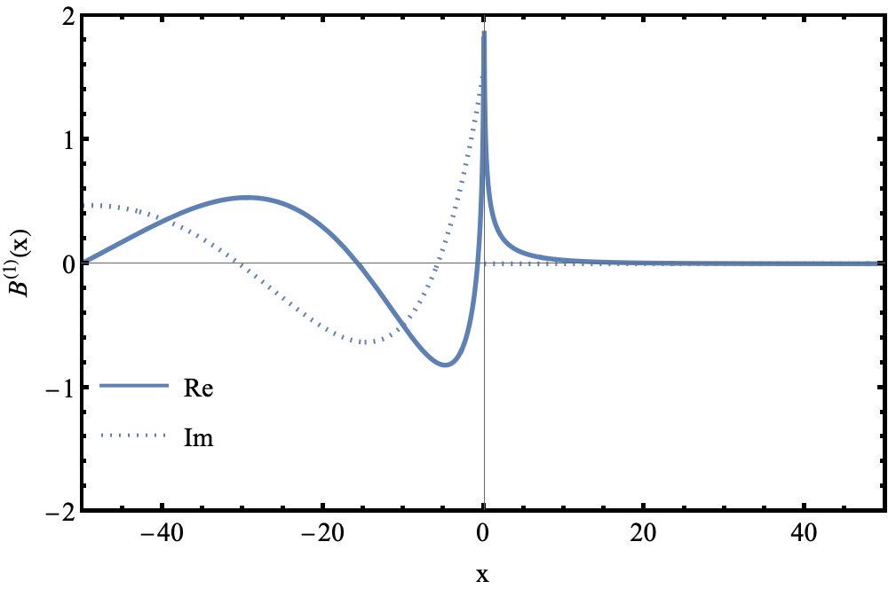
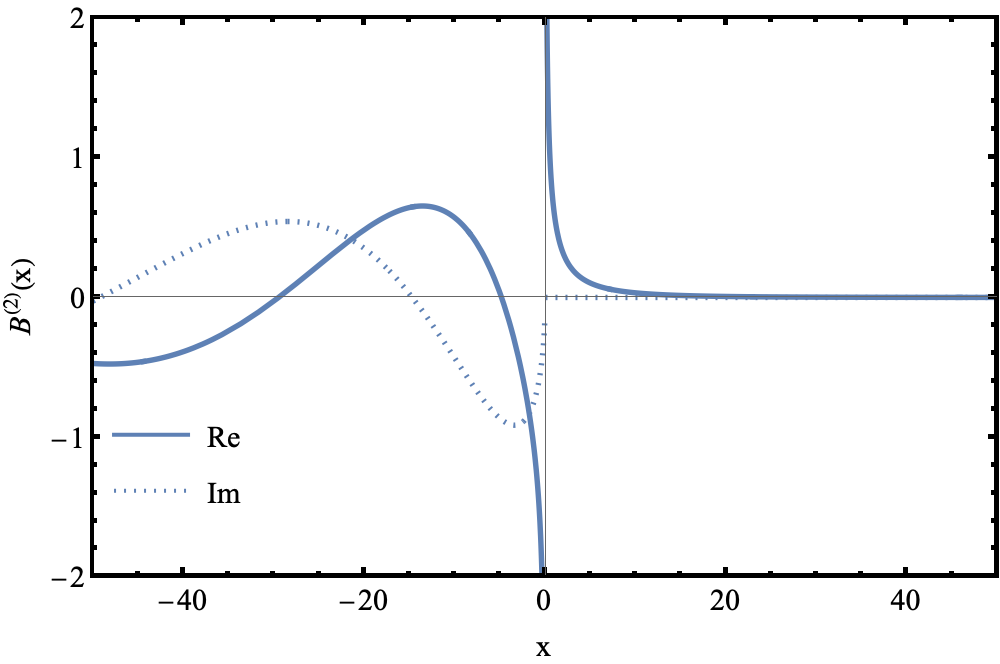
Figure 4: The Bessel functions $B^{(1)}$ (left) and $B^{(2)}$ (right).

The aforementioned divergences of $B^{(2)}$ ought to cancel, since they are from an integrable singularity as shown in Eq. (37); the integrand takes the same values in magnitude but with opposite signs at $x=\epsilon$ and $x=-\epsilon$, where $\epsilon$ is a tiny parameter. We then decompose the function $B^{(2)}(x)$ into two terms, $B^{(2)}(x)-\text{Sign}(x)/\sqrt{|x|}$ and $\text{Sign}(x)/\sqrt{|x|}$, as depicted in Fig. 5. The former is finite everywhere, whose integration is convergent and can be evaluated reliably by the VEGAS+. The latter is divergent at $x=0$ but antisymmetric about the origin. Therefore, the contributions to its integral from the intervals $(-\epsilon,0)$ and $(0,\epsilon)$ in $x$ are expected to cancel exactly and negligible. This operation replaces the integrations involving $F_{2,3,4}$ by the sum of two pieces, one with $B^{(2)}(x)-\text{Sign}(x)/\sqrt{|x|}$ in the entire range of $x$ and the other with $\text{Sign}(x)/\sqrt{|x|}$ in the region outside $(-\epsilon,\epsilon)$. It has been checked that the cut parameter $\epsilon$ within the range $0.0005\sim 0.005$ leads to accurate outcomes with controllable uncertainties. Here we set $\epsilon=0.001$, for which the errors in the real parts of the $T(d5)$ contributions indeed decrease as $1/\sqrt{N_{ev}}$, as indicated in Fig. 6. It confirms the effectiveness of our algorithm.

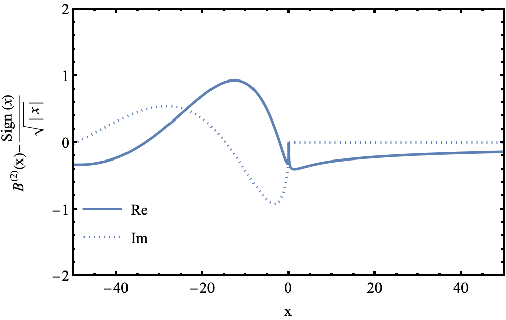
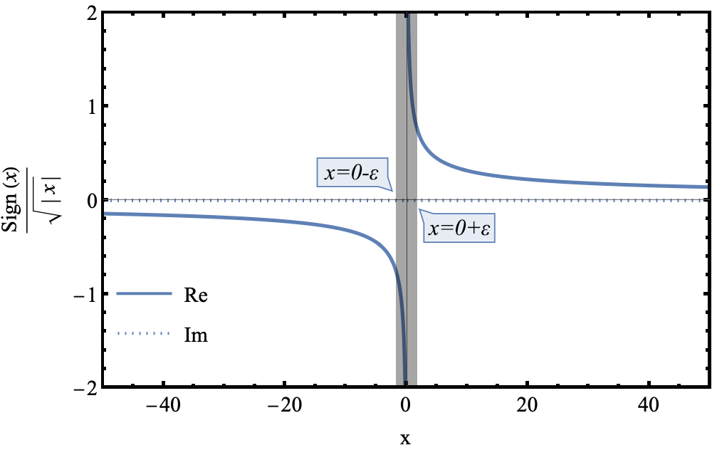
Figure 5: The function $B^{(2)}(x)-\text{Sign}(x)/\sqrt{|x|}$ (left) ; the function $\text{Sign}(x)/\sqrt{|x|}$ (right).

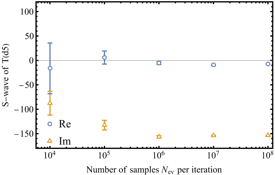
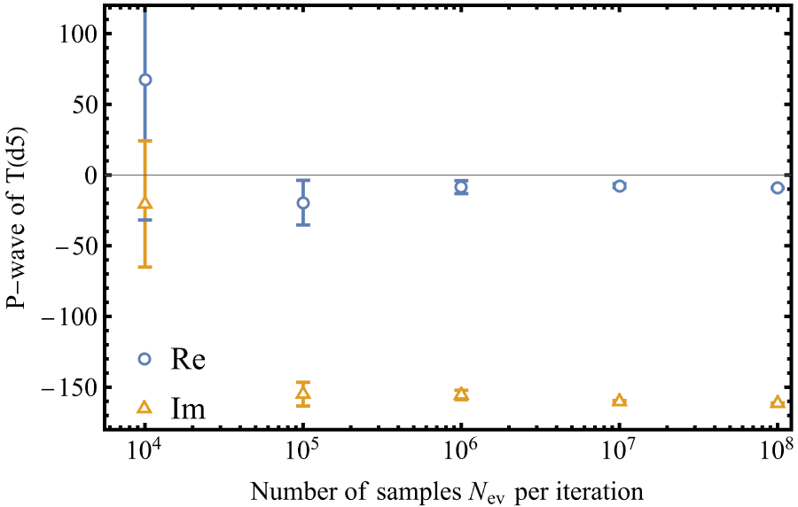
Figure 6: Same as Fig. 3 but the integrals are treated under our algorithm.

III Numerical Results

III.1 Two-body $\Lambda_{b}\to ph$ decays

We start with the invariant amplitude of the $\Lambda_{b}(\frac{1}{2}^{+})\to p(\frac{1}{2}^{+})h(0^{-})$ decay Cheng:1996cs, $h=\pi^{-}$ or $K^{-}$,

$$\mathcal{A}=i\bar{u}_{p}(p_{p})(S+P\gamma_{5})u_{\Lambda_{b}}(p_{\Lambda_{b}}),$$ (38)

where $u_{p}$ is the proton spinor, and $S$ ($P$) denotes the parity-violating $S$-wave (parity-conserving $P$-wave) amplitude. CPVs are generated by the interference between the contributions of the tree operators $\mathcal{T}$ and the penguin operators $\mathcal{P}$. The $S$- and $P$-wave amplitudes are split into Han:2024kgz

$$\begin{split}S&=\lambda_{\mathcal{T}}|S_{\mathcal{T}}|e^{i\delta_{\mathcal{T}}^{S}}+\lambda_{\mathcal{P}}|S_{\mathcal{P}}|e^{i\delta_{\mathcal{P}}^{S}},\\ P&=\lambda_{\mathcal{T}}|P_{\mathcal{T}}|e^{i\delta_{\mathcal{T}}^{P}}+\lambda_{\mathcal{P}}|P_{\mathcal{P}}|e^{i\delta_{\mathcal{P}}^{P}},\end{split}$$ (39)

where $\delta$’s represent the strong phases, and $\lambda_{\mathcal{T}}=V_{ub}V_{ud(s)}^{*}$ and $\lambda_{\mathcal{P}}=V_{tb}V_{td(s)}^{*}$ are the products of the CKM matrix elements. It is reminded that the $S$-wave amplitude flips sign under the $C$ transformation, but the $P$-wave one does not Wang:2024qff,

$$\begin{split}S\to\bar{S}&=-\lambda_{\mathcal{T}}^{\ast}|S_{\mathcal{T}}|e^{i\delta_{\mathcal{T}}^{S}}-\lambda_{\mathcal{P}}^{\ast}|S_{\mathcal{P}}|e^{i\delta_{\mathcal{P}}^{S}},\\ P\to\bar{P}&=\lambda_{\mathcal{T}}^{\ast}|P_{\mathcal{T}}|e^{i\delta_{\mathcal{T}}^{P}}+\lambda_{\mathcal{P}}^{\ast}|P_{\mathcal{P}}|e^{i\delta_{\mathcal{P}}^{P}}.\end{split}$$ (40)

It is equivalent to formulate the decay $\Lambda_{b}\to ph$ in terms of the helicity amplitudes, defined as

$$H_{\lambda_{p},\lambda_{h}}=\langle p(\lambda_{p})h(\lambda_{h})|H_{W}|\Lambda_{b}(\lambda_{\Lambda_{b}})\rangle.$$ (41)

The $\Lambda_{b}$ spin component obeys $\lambda_{\Lambda_{b}}=\lambda_{p}-\lambda_{h}$ with the proton helicity $\lambda_{p}$ and the meson spin $\lambda_{h}$. The helicity amplitudes $H_{\lambda_{p},\lambda_{h}}$ are related to the partial-wave amplitudes via

$$H_{1/2,0} =-iM_{+}S+iM_{-}P,$$

$$H_{-1/2,0} =-iM_{+}S-iM_{-}P,$$ (42)

with the coefficients $M_{\pm}^{2}\equiv(m_{\Lambda_{b}}\pm m_{p})^{2}-m_{h}^{2}=2m_{\Lambda_{b}}(E_{p}\pm m_{p})$, $E_{p}$ being the proton energy.

We calculate the contributions from all diagrams to the invariant amplitudes $S_{\mathcal{T},\mathcal{P}}$ and $P_{\mathcal{T},\mathcal{P}}$ in Eq. (39), including their strong phases, for the $\Lambda_{b}\to p\pi^{-}$, $pK^{-}$ decays in the PQCD approach. The results can be transformed into the helicity amplitudes in Eq. (42) straightforwardly. It is worth mentioning that the nonfactorizable diagrams from the topologies $PC_{2}$ and $PE_{1}^{u}$ are evaluated for the first time. Our predictions for the $\Lambda_{b}\to p\pi^{-}$ ($pK^{-}$) amplitudes are presented in Tables 5 and 6 (7 and 8), where only the central values are given for clarity.

The contributions to the decay amplitudes have been categorized according to topologies in the above tables. The external-$W$ emission topology $T$ is further divided into the factorizable part $T^{f}$ and the non-factorizable part $T^{nf}$, and the same division applies to the $PC_{1}$ topology. The topological amplitudes, excluding the CKM matrix elements, respect the hierarchy relations,

$$\begin{split}|T^{f}|\gg|E_{2}|\gtrsim&|PC_{1}^{f}|\gtrsim|T^{nf}|>|C_{2}|>|PC_{2}|>|B|\\ &\gtrsim|PE_{1}^{u}|>|PE_{1}^{d}|\sim|PB|\sim|PE_{2}|\sim|PC_{1}^{nf}|\;\text{ ($S$ wave)},\\ |T^{f}|\gg|T^{nf}|&\gg|E_{2}|>|C_{2}|>|B|>|PC_{2}|\gtrsim|PC_{1}^{nf}|\\ &\gtrsim|PE_{1}^{u}|>|PC_{1}^{f}|>|PE_{1}^{d}|\sim|P^{B}|\sim|PE_{2}|\;\text{ ($P$ wave)},\end{split}$$ (43)

with the explicit relative ratios,

$$\begin{split}&\frac{|C_{2}|}{|T|}=0.042,\quad\frac{|E_{2}|}{|T|}=0.095,\quad\frac{|B|}{|T|}=0.014\;\text{ ($S$ wave)},\\ &\frac{|C_{2}|}{|T|}=0.041,\quad\frac{|E_{2}|}{|T|}=0.072,\quad\frac{|B|}{|T|}=0.024\text{ ($P$ wave)},\\ \end{split}$$ (44)

for the $\Lambda_{b}\to p\pi^{-}$ mode. Likewise, we have

$$\begin{split}&|T^{f}|\gg|E_{2}|\gtrsim|PC_{1}^{f}|\gtrsim|T^{nf}|>|PE_{1}^{u}|>|PE_{1}^{d}|>|PC_{1}^{nf}|\;\text{ ($S$ wave)},\\ &|T^{f}|\gg|T^{nf}|\gg|E_{2}|>|PC_{1}^{nf}|\gtrsim|PE_{1}^{u}|>|PC_{1}^{f}|>|PE_{1}^{d}|\;\text{ ($P$ wave)},\end{split}$$ (45)

$$\frac{|E_{2}|}{|T|}=0.104\;\text{ ($S$ wave)},\quad\frac{|E_{2}|}{|T|}=0.076\;\text{ ($P$ wave)}.$$ (46)

for the $\Lambda_{b}\to pK^{-}$ mode. It is seen that Eqs. (43) and (45) are consistent with those from the SCET Leibovich:2003tw.

The $\Lambda_{b}\to p\pi^{-},pK^{-}$ decays share the same topologies $T$ and $E_{2}$, allowing a quantitative assessment on the SU(3)${}_{F}$ flavor symmetry breaking effects. The ratios

$$\begin{split}&\frac{|T^{f}(pK)|}{|T^{f}(p\pi)|}=1.22,\quad\frac{|T^{nf}(pK)|}{|T^{nf}(p\pi)|}=1.03,\quad\frac{|E_{2}(pK)|}{|E_{2}(p\pi)|}=1.33\text{ (S wave)},\\ &\frac{|T^{f}(pK)|}{|T^{f}(p\pi)|}=1.23,\quad\frac{|T^{nf}(pK)|}{|T^{nf}(p\pi)|}=1.28,\quad\frac{|E_{2}(pK)|}{|E_{2}(p\pi)|}=1.29\text{ (P wave)}.\end{split}$$ (47)

imply that the SU(3)${}_{F}$ breaking effects reach roughly $30\%$, similar to the case of $B$ meson decays Cheng:2011qh. The breaking effects primarily originate from the meson decay constants in the factorizable $T_{f}$ topology because of $|T^{f}(pK)|/|T^{f}(p\pi)|\approx f_{K}/f_{\pi}$, and from the meson DAs in the the other topologies.

Table 5: Invariant amplitudes of the $\Lambda_{b}\to p\pi^{-}$ decay classified by topologies without the CKM matrix elements.

$\Lambda_{b}\to p\pi^{-}$	$|S|$	$\delta^{S}(^{\circ})$	Real($S$)	Imag($S$)	$|P|$	$\delta^{P}(^{\circ})$	Real($P$)	Imag($P$)
$T^{f}$	707.17	0.00	707.17	0.00	1004.44	0.00	1004.44	0.00
$T^{nf}$	51.72	-96.64	-5.98	-51.38	267.72	-97.92	-36.90	-265.17
$T^{f}+T^{nf}$	703.07	-4.19	701.19	-51.38	1003.22	-15.33	967.54	-265.17
$C_{2}$	29.37	154.96	-26.61	12.43	41.51	179.80	-41.51	0.14
$E_{2}$	66.94	-145.26	-55.01	-38.14	72.58	119.94	-36.23	62.89
$B$	10.40	112.64	-4.00	9.60	23.65	-122.56	-12.73	-19.93
Tree	619.26	-6.26	615.57	-67.49	904.75	-14.21	877.08	-222.06
$PC_{1}^{f}$	58.44	0.00	58.44	0.00	2.90	0.00	2.90	0.00
$PC_{1}^{nf}$	1.24	-115.38	-0.53	-1.12	11.16	-95.25	-1.02	-11.11
$PC_{1}^{f}+PC_{1}^{nf}$	57.91	-1.11	57.90	-1.12	11.27	-80.38	1.88	-11.11
$PC_{2}$	13.36	-116.10	-5.88	-12.00	14.93	71.96	4.62	14.20
$PE_{1}^{u}$	9.48	-87.62	0.39	-9.47	8.83	114.44	-3.65	8.04
$PB$	1.36	-51.30	0.85	-1.06	1.55	-159.86	-1.46	-0.53
$PE_{1}^{d}+PE_{2}$	3.87	-98.18	-0.55	-3.83	1.41	-12.55	1.37	-0.31
Penguin	59.45	-27.54	52.71	-27.49	10.65	74.93	2.77	10.28

Table 6: Helicity amplitudes of the $\Lambda_{b}\to p\pi^{-}$ decay classified by topologies without the CKM matrix elements.

$\Lambda_{b}\to p\pi^{-}$	$|H_{\frac{1}{2},0}|$	$\delta(H_{\frac{1}{2},0})^{\circ}$	Real($H_{\frac{1}{2},0}$)	Imag($H_{\frac{1}{2},0}$)	$|H_{-\frac{1}{2},0}|$	$\delta(H_{-\frac{1}{2},0})^{\circ}$	Real($H_{-\frac{1}{2},0}$)	Imag($H_{-\frac{1}{2},0}$)
$T^{f}$	65.30	90.00	0.00	65.30	9344.10	-90.00	0.00	-9344.10
$T^{nf}$	914.77	-8.40	904.96	-133.62	1593.23	172.35	-1579.06	212.04
$T^{f}+T^{nf}$	907.53	-4.32	904.96	-68.32	9267.57	-99.81	-1579.06	-9132.06
$C_{2}$	83.29	-13.80	80.89	-19.87	378.05	77.44	82.24	369.00
$E_{2}$	577.41	160.66	-544.83	191.24	532.44	85.22	44.34	530.59
$B$	159.82	-12.04	156.30	-33.35	91.09	109.50	-30.40	85.87
Tree	601.38	6.66	597.33	69.70	8280.47	-100.32	-1482.88	-8146.61
$PC_{1}^{f}$	369.76	-90.00	0.00	-369.76	396.97	-90.00	0.00	-396.97
$PC_{1}^{nf}$	44.70	-1.64	44.68	-1.28	60.01	172.07	-59.43	8.28
$PC_{1}^{f}+PC_{1}^{nf}$	373.72	-83.13	44.68	-371.04	393.21	-98.69	-59.43	-388.69
$PC_{2}$	157.24	157.48	-145.25	60.24	20.86	125.84	-12.21	16.91
$PE_{1}^{u}$	101.73	-168.84	-99.80	-19.70	28.48	149.33	-24.50	14.53
$PB$	13.17	-109.70	-4.44	-12.40	9.53	172.34	-9.45	1.27
$PE_{1}^{d}+PE_{2}$	25.76	157.05	-23.72	10.04	26.73	-173.96	-26.58	-2.81
Penguin	403.75	-124.47	-228.52	-332.85	382.37	-110.22	-132.18	-358.80

Table 7: Same as Table 5 but for the $\Lambda_{b}\to pK^{-}$ decay.

$\Lambda_{b}\to pK^{-}$	$|S|$	$\delta^{S}(^{\circ})$	Real($S$)	Imag($S$)	$|P|$	$\delta^{P}(^{\circ})$	Real($P$)	Imag($P$)
$T^{f}$	865.44	0.00	865.44	0.00	1230.64	0.00	1230.64	0.00
$T^{nf}$	53.41	-102.81	-11.84	-52.08	343.23	-96.76	-40.43	-340.84
$T^{f}+T^{nf}$	855.18	-3.49	853.60	-52.08	1238.05	-15.98	1190.21	-340.84
$E_{2}$	89.06	-138.10	-66.28	-59.48	94.13	122.31	-50.31	79.56
Tree	795.18	-8.06	787.31	-111.55	1169.46	-12.91	1139.90	-261.28
$PC_{1}^{f}$	76.43	0.00	76.43	0.00	3.30	180.00	-3.30	0.00
$PC_{1}^{nf}$	1.14	-134.10	-0.79	-0.82	13.85	-94.36	-1.05	-13.81
$PC_{1}^{f}+PC_{1}^{nf}$	75.64	-0.62	75.64	-0.82	14.48	-107.50	-4.35	-13.81
$PE_{1}^{u}$	11.80	-89.53	0.10	-11.80	11.02	115.62	-4.76	9.93
$PE_{1}^{d}$	7.53	-101.53	-1.50	-7.38	2.67	51.53	1.66	2.09
Penguin	76.88	-15.08	74.23	-20.00	7.66	-166.53	-7.45	-1.79

Table 8: Same as Table 6 but for the $\Lambda_{b}\to pK^{-}$ decay.

$\Lambda_{b}\to pK^{-}$	$|H_{\frac{1}{2},0}|$	$\delta(H_{\frac{1}{2},0})^{\circ}$	Real($H_{\frac{1}{2},0}$)	Imag($H_{\frac{1}{2},0}$)	$|H_{-\frac{1}{2},0}|$	$\delta(H_{-\frac{1}{2},0})^{\circ}$	Real($H_{-\frac{1}{2},0}$)	Imag($H_{-\frac{1}{2},0}$)
$T^{f}$	71.74	90.00	0.00	71.74	11397.55	-90.00	0.00	-11397.55
$T^{nf}$	1252.42	-5.08	1247.50	-110.90	1947.26	172.15	-1929.02	265.90
$T^{f}+T^{nf}$	1248.12	-1.80	1247.50	-39.17	11297.55	-99.83	-1929.02	-11131.65
$E_{2}$	785.62	165.31	-759.92	199.29	668.39	91.58	-18.44	668.13
Tree	513.20	18.18	487.58	160.12	10643.20	-100.54	-1947.46	-10463.51
$PC_{1}^{f}$	515.50	-90.00	0.00	-515.50	484.74	-90.00	0.00	-484.74
$PC_{1}^{nf}$	59.00	0.28	59.00	0.29	70.45	171.76	-69.72	10.10
$PC_{1}^{f}+PC_{1}^{nf}$	518.58	-83.47	59.00	-515.22	479.73	-98.36	-69.72	-474.64
$PE_{1}^{u}$	125.61	-169.53	-123.52	-22.83	37.72	145.13	-30.95	21.57
$PE_{1}^{d}$	60.63	163.13	-58.02	17.60	38.56	176.88	-38.51	2.10
Penguin	534.68	-103.25	-122.54	-520.44	471.96	-107.15	-139.17	-450.97

A hierarchy relation exists between the helicity amplitudes $H_{-1/2,0}$ and $H_{1/2,0}$ from the factorizable topology $T^{f}$, as manifested in Tables. 6 and 8. The proton spin tends to be anti-parallel to its momentum due to the chiral current $(V-A)$ in weak interaction, granting the dominance of $H_{-1/2,0}$ over $H_{1/2,0}$.

Tables. 5 and 7 and the hierarchy relations in Eqs. (43) and (45) declare that the factorizable penguin contribution to the $P$-wave is much lower than to the $S$-wave, i.e., $|PC_{1}^{f}|^{\text{$P$-wave}}\ll|PC_{1}^{f}|^{\text{$S$-wave}}$. This feature is attributed to the current structures of the penguin operators; the matrix element for the factorizable penguin $PC_{1}^{f}$ from the $(V-A)\otimes(V-A)$ operators like $O_{4}$ is written, in the factorization hypothesis, as

$$\begin{split}\langle p\pi^{-}|O_{4}|\Lambda_{b}\rangle=&\langle p\pi^{-}|(\bar{d}_{\alpha}b_{\beta})_{V-A}(\bar{u}_{\beta}u_{\alpha})_{V-A}|\Lambda_{b}\rangle\\ =&\langle\pi^{-}|(\bar{d}u)_{V-A}|0\rangle\left[\langle p|(\bar{u}b)_{V}|\Lambda_{b}\rangle-\langle p|(\bar{u}b)_{A}|\Lambda_{b}\rangle\right].\end{split}$$ (48)

For the $(V-A)\otimes(V+A)$ operators like $O_{6}$, the corresponding matrix element is approximated by

$$\begin{split}\langle p\pi^{-}|O_{6}|\Lambda_{b}\rangle=&\langle p\pi^{-}|(\bar{d}_{\alpha}b_{\beta})_{V-A}(\bar{u}_{\beta}u_{\alpha})_{V+A}|\Lambda_{b}\rangle\\ =&-2\langle\pi^{-}|(\bar{d}u)_{S+P}|0\rangle\langle p|(\bar{u}b)_{S-P}|\Lambda_{b}\rangle\\ =&\langle\pi^{-}|(\bar{d}u)_{V-A}|0\rangle\Big{[}\frac{2m_{\pi}^{2}}{(m_{b}-m_{u})(m_{u}+m_{d})}\langle p|(\bar{u}b)_{V}|\Lambda_{b}\rangle\\ &+\frac{2m_{\pi}^{2}}{(m_{b}+m_{u})(m_{u}+m_{d})}\langle p|(\bar{u}b)_{A}|\Lambda_{b}\rangle\Big{]}\\ =&\langle\pi^{-}|(\bar{d}u)_{V-A}|0\rangle\left(R_{1}^{\pi}\langle p|(\bar{u}b)_{V}|\Lambda_{b}\rangle+R_{2}^{\pi}\langle p|(\bar{u}b)_{A}|\Lambda_{b}\rangle\right),\end{split}$$ (49)

with the chiral factors $R_{1}^{\pi}\equiv\frac{2m_{\pi}^{2}}{(m_{b}-m_{u})(m_{u}+m_{d})}$ and $R_{2}^{\pi}\equiv\frac{2m_{\pi}^{2}}{(m_{b}+m_{u})(m_{u}+m_{d})}$.

The $S$- and $P$-wave $PC_{1}^{f}$ amplitudes then read

$$\begin{split}(PC_{1}^{f})^{\text{$S$-wave}}=&-\frac{G_{F}}{\sqrt{2}}f_{h}V_{tb}V_{td}^{\ast}\left[\frac{C_{3}}{3}+C_{4}+\frac{C_{9}}{3}+C_{10}+R_{1}^{\pi}(\frac{C_{5}}{3}+C_{6}+\frac{C_{7}}{3}+C_{8})\right]\\ &\Big{[}f_{1}(m_{h}^{2})(m_{\Lambda_{b}}-m_{p})+f_{3}(m_{h}^{2})m_{h}^{2}\Big{]},\\ (PC_{1}^{f})^{\text{$P$-wave}}=&-\frac{G_{F}}{\sqrt{2}}f_{h}V_{tb}V_{td}^{\ast}\left[\frac{C_{3}}{3}+C_{4}+\frac{C_{9}}{3}+C_{10}-R_{2}^{\pi}(\frac{C_{5}}{3}+C_{6}+\frac{C_{7}}{3}+C_{8})\right]\\ &\Big{[}g_{1}(m_{h}^{2})(m_{\Lambda_{b}}+m_{p})-g_{3}(m_{h}^{2})m_{h}^{2}\Big{]},\end{split}$$ (50)

respectively, where the form factors $f_{1,3}$ and $g_{1,3}$ are defined in terms of the matrix element $\langle p|\bar{u}\gamma_{\mu}b|\Lambda_{b}\rangle=\bar{u}_{p}(f_{1}\gamma_{\mu}+f_{2}i\sigma_{\mu\nu}q^{\nu}+f_{3}q_{\mu})u_{\Lambda_{b}}$ and $\langle p|\bar{u}\gamma_{\mu}\gamma_{5}b|\Lambda_{b}\rangle=\bar{u}_{p}(g_{1}\gamma_{\mu}+g_{2}i\sigma_{\mu\nu}q^{\nu}+g_{3}q_{\mu})\gamma_{5}u_{\Lambda_{b}}$. The chiral factors $R_{1,2}^{\pi}$ are of $\mathcal{O}(1)$, so the negative sign of the $R_{2}^{\pi}$ piece in the second expression of Eq. (50) results in destruction. As a consequence, the $S$-wave $PC_{1}^{f}$ is enhanced, while the $P$-wave one is suppressed.

It is observed from the amplitudes in Appendix. B that specific combinations of the hadron DAs may produce opposite signs between the $S$ and $P$ waves. For instance, Eq. (97) from the combination of the $\Lambda_{b}$ twist-2, proton twist-3 and meson twist-2 DAs yields

$$\begin{split}&M_{T_{nf}(c7)}^{(V-A)\otimes(V-A)}(\Lambda_{b}~\text{twist-2-proton twist-3-meson twist-2})\\ =&8m_{\Lambda_{b}}^{4}(x_{3}-y)(-2A_{1}\psi_{2}(-1+x_{2}+y)+2\psi_{2}(2T_{1}+V_{1})(-1+x_{2}+y))\phi_{m}^{A}\\ &+8m_{\Lambda_{b}}^{4}(x_{3}-y)(-2A_{1}\psi_{2}(-1+x_{2}+y)+2\psi_{2}(2T_{1}+V_{1})(-1+x_{2}+y))\phi_{m}^{A}\gamma_{5},\end{split}$$ (51)

where the $S$-wave (first) piece and the $P$-wave (second) piece have the same sign. Nevertheless, the two partial waves are opposite in sign in the combination of the $\Lambda_{b}$ twist-3, proton twist-3 and meson twist-2 DAs,

$$\begin{split}&M_{T_{nf}(c7)}^{(V-A)\otimes(V-A)}(\Lambda_{b}~\text{twist-3+proton twist-3+meson twist-2})\\ =&8m_{\Lambda_{b}}^{4}(x_{3}-y)(A_{1}\psi_{3}^{-+}x_{2}^{\prime}+V_{1}\psi_{3}^{-+}x_{2}^{\prime})\phi_{m}^{A}\\ &-8m_{\Lambda_{b}}^{4}(x_{3}-y)(A_{1}\psi_{3}^{-+}x_{2}^{\prime}+V_{1}\psi_{3}^{-+}x_{2}^{\prime})\phi_{m}^{A}\gamma_{5}.\end{split}$$ (52)

This distinction arises from the different numbers of $\gamma_{5}$ for the $S$ and $P$ waves endowed by the vector and axial-vector currents in weak interaction and by the Dirac structures of the hadron DAs.

We survey all combinations of the DAs, and decide the relative signs between the $S$- and $P$-wave amplitudes as exhibited in Table 9, where the symbol ‘$+$’ (‘$-$’) means the same (opposite) sign. It is interesting that the relative sign between the $S$ and $P$ waves alternates with the twists of the $\Lambda_{b}$ or proton DAs. This feature holds for all Feynman diagrams and all types of weak interaction vertices. The net interference between the $S$- and $P$-wave amplitudes for a topology is then determined by the dominant Feynman diagram and DA combination involved. This accounts for the notable fluctuation of the strong phases in Tables. 5 and 7. The different strong phases impact the predictions for CPVs, which will be explored in the following subsections.

meson twist-2	proton twist-3	proton twist-4	proton twist-5	proton twist-6
$\Lambda_{b}$ twist-2	+	-	+	-
$\Lambda_{b}$ twist-3	-	+	-	+
$\Lambda_{b}$ twist-4	+	-	+	-
meson twist-3	proton twist-3	proton twist-4	proton twist-5	proton twist-6
$\Lambda_{b}$ twist-2	-	+	-	+
$\Lambda_{b}$ twist-3	+	-	+	-
$\Lambda_{b}$ twist-4	-	+	-	+

Table 9: Relative signs between the $S$- and $P$-wave amplitudes for various twist combinations of the $\Lambda_{b}$ and proton DAs.

With the obtained amplitudes, we predict the various observables associated with the $\Lambda_{b}\to p\pi^{-},pK^{-}$ decays as elaborated below. The outcomes are assembled in Table 10, where the first three errors are from the inputs in the $\Lambda_{b}$, proton and meson DAs, respectively, and the fourth one stems from varying the renormalization scale of the Wilson coefficients in Table 1. The uncertainties from the CKM matrix elements are negligible relative to the above sources.

Table 10: Observables associated with the $\Lambda_{b}\to p\pi^{-},pK^{-}$ decays. The percentages in the parentheses stand for the proportions of the partial-wave CPVs to the direct CPVs.

	$Br(\times 10^{-6})$
$\Lambda_{b}\to p\pi^{-}$	$3.34^{+2.53+1.33+0.10+0.47}_{-1.30-1.10-0.11-0.14}$
$\Lambda_{b}\to pK^{-}$	$2.83^{+2.17+1.17+0.49+2.19}_{-1.05-0.92-0.37-0.66}$
	$A_{CP}^{dir}$	$A_{CP}^{S}(\kappa_{S})$	$A_{CP}^{P}(\kappa_{P})$
$\Lambda_{b}\to p\pi^{-}$	$0.05^{+0.00+0.00+0.00+0.02}_{-0.02-0.01-0.02-0.01}$	$0.17^{+0.01+0.01+0.03+0.04}_{-0.04-0.04-0.07-0.04}(49\%)$	$-0.06^{+0.01+0.03+0.02+0.00}_{-0.02-0.03-0.03-0.01}(51\%)$
$\Lambda_{b}\to pK^{-}$	$-0.06^{+0.01+0.01+0.02+0.00}_{-0.01-0.01-0.01-0.00}$	$-0.05^{+0.02+0.02+0.04+0.00}_{-0.02-0.01-0.03-0.00}(94\%)$	$-0.21^{+0.07+0.23+0.29+0.04}_{-0.15-0.33-0.27-0.01}(6\%)$
	$\alpha$	$A_{CP}^{\alpha}$	$\langle\alpha\rangle$
$\Lambda_{b}\to p\pi^{-}$	$-0.94^{+0.00+0.02+0.01+0.03}_{-0.02-0.02-0.02-0.02}$	$0.02^{+0.00+0.01+0.00+0.01}_{-0.01-0.01-0.01-0.01}$	$-0.96^{+0.00+0.01+0.01+0.02}_{-0.00-0.01-0.01-0.01}$
$\Lambda_{b}\to pK^{-}$	$0.23^{+0.04+0.02+0.10+0.15}_{-0.03-0.05-0.12-0.07}$	$0.04^{+0.02+0.02+0.01+0.01}_{-0.02-0.03-0.01-0.01}$	$0.20^{+0.02+0.01+0.11+0.14}_{-0.02-0.02-0.12-0.06}$
	$\beta$	$A_{CP}^{\beta}$	$\langle\beta\rangle$
$\Lambda_{b}\to p\pi^{-}$	$0.34^{+0.00+0.05+0.01+0.07}_{-0.06-0.06-0.06-0.05}$	$0.22^{+0.00+0.00+0.03+0.07}_{-0.01-0.01-0.04-0.03}$	$0.12^{+0.00+0.05+0.03+0.00}_{-0.05-0.05-0.04-0.02}$
$\Lambda_{b}\to pK^{-}$	$-0.39^{+0.03+0.08+0.08+0.12}_{-0.01-0.04-0.07-0.01}$	$-0.44^{+0.01+0.01+0.02+0.08}_{-0.00-0.00-0.01-0.04}$	$0.05^{+0.03+0.08+0.07+0.04}_{-0.01-0.05-0.07-0.02}$
	$\gamma$	$A_{CP}^{\gamma}$	$\langle\gamma\rangle$
$\Lambda_{b}\to p\pi^{-}$	$0.09^{+0.02+0.04+0.04+0.04}_{-0.04-0.06-0.06-0.01}$	$0.11^{+0.01+0.02+0.03+0.03}_{-0.02-0.03-0.04-0.02}$	$-0.02^{+0.01+0.02+0.01+0.01}_{-0.02-0.04-0.01-0.00}$
$\Lambda_{b}\to pK^{-}$	$0.89^{+0.02+0.04+0.04+0.00}_{-0.01-0.02-0.05-0.01}$	$0.02^{+0.02+0.05+0.04+0.00}_{-0.01-0.03-0.04-0.00}$	$0.87^{+0.00+0.01+0.02+0.00}_{-0.00-0.01-0.02-0.01}$

The decay width is written as

$$\Gamma=\frac{p_{c}}{8\pi m_{\Lambda_{b}}^{2}}\left\{M_{+}^{2}|S|^{2}+M_{-}^{2}|P|^{2}\right\}=\frac{p_{c}}{16\pi m_{\Lambda_{b}}^{2}}\left(|H_{1/2,0}|^{2}+|H_{-1/2,0}|^{2}\right),$$ (53)

where

$$\begin{split}p_{c}&=\sqrt{[(m_{\Lambda_{b}}+m_{p})^{2}-m_{h}^{2}][(m_{\Lambda_{b}}-m_{p})^{2}-m_{h}^{2}]}/(2m_{\Lambda_{b}}),\end{split}$$ (54)

is the momentum of either the proton or the meson in the rest frame of the $\Lambda_{b}$ baryon. The predicted $\Lambda_{b}\to p\pi^{-}$ and $\Lambda_{b}\to pK^{-}$ branching ratios are a bit lower than the data $Br(\Lambda_{b}\to p\pi^{-})=(4.6\pm 0.8)\times 10^{-6}$ and $Br(\Lambda_{b}\to pK^{-})=(5.5\pm 1.0)\times 10^{-6}$. We suspect that the discrepancy is attributed to higher-order corrections, in particular those to the non-factorizable topologies. The factorizable contributions have been more or less fixed by the measured $\Lambda_{b}\to p\mu\bar{\nu}_{\mu}$ and $\Lambda_{b}\to pD_{s}^{-}$ branching ratios. The uncertainty arising from the Wilson coefficients for the $\Lambda_{b}\to pK^{-}$ decay is larger than for $\Lambda_{b}\to p\pi^{-}$, suggesting that higher-order contributions are more important in penguin-dominant modes.

The $\Lambda_{b}\to p\pi^{-},pK^{-}$ decays share the same inputs from the $\Lambda_{b}$ and proton DAs, so the errors from these sources are suppressed in the difference of the branching ratios,

$$\begin{split}\Delta Br(\Lambda_{b}\to pK^{-}/\pi^{-})&\equiv Br(\Lambda_{b}\to pK^{-})-Br(\Lambda_{b}\to p\pi^{-})\\ &=(-0.51^{+0.25+0.20+0.50+1.72}_{-0.36-0.17-0.38-0.52})\times 10^{-6}.\end{split}$$ (55)

Though the errors from the meson DAs and the Wilson coefficients keep sizable, Eq. (55) indicates that the $\Lambda_{b}\to pK^{-}$ branching ratio is higher than the $\Lambda_{b}\to p\pi^{-}$ one. The discrepancy between Eq. (55) and the LHCb measurements may be also resolved by including higher-order corrections, as hinted by the crucial effects from varying the renormalization scale of the Wilson coefficients.

According to the definition for the direct CPV of the $\Lambda_{b}\to ph$ decay,

$$A_{CP}^{dir}(\Lambda_{b}\to ph)\equiv\frac{\Gamma(\Lambda_{b}\to ph)-\bar{\Gamma}(\bar{\Lambda}_{b}\to\bar{p}\bar{h})}{\Gamma(\Lambda_{b}\to ph)+\bar{\Gamma}(\bar{\Lambda}_{b}\to\bar{p}\bar{h})},$$ (56)

we have the explicit expression

$$A_{CP}^{dir}=\frac{-2M_{+}^{2}|S_{\mathcal{T}}|^{2}r_{S}\sin\Delta\phi\sin\Delta\delta_{S}-2M_{-}^{2}|P_{\mathcal{T}}|^{2}r_{P}\sin\Delta\phi\sin\Delta\delta_{P}}{M_{+}^{2}|S_{\mathcal{T}}|^{2}(1+r_{S}^{2}+2r_{S}\cos\Delta\phi\cos\Delta\delta_{S})+M_{-}^{2}|P_{\mathcal{T}}|^{2}(1+r_{P}^{2}+2r_{P}\cos\Delta\phi\cos\Delta\delta_{P})},$$ (57)

where $r_{S}=|\lambda_{\mathcal{P}}S_{\mathcal{P}}|/|\lambda_{\mathcal{T}}S_{\mathcal{T}}|$ ($r_{P}=|\lambda_{\mathcal{P}}P_{\mathcal{P}}|/|\lambda_{\mathcal{T}}P_{\mathcal{T}}|$) is the ratio of the penguin amplitude to the tree amplitude for the $S$ ($P$) wave, the difference of the weak phases $\Delta\phi\equiv\text{arg}(\lambda_{\mathcal{P}})-\text{arg}(\lambda_{\mathcal{T}})$ is identical for both waves, and $\Delta\delta_{S}=\delta_{\mathcal{P}}^{S}-\delta_{\mathcal{T}}^{S}$ ($\Delta\delta_{P}=\delta_{\mathcal{P}}^{P}-\delta_{\mathcal{T}}^{P}$) is the difference of the strong phases for the $S$ ($P$) wave. It is trivial to construct the partial-wave CPVs,

$$\begin{split}A_{CP}^{S}\equiv&\frac{|S|^{2}-|\bar{S}|^{2}}{|S|^{2}+|\bar{S}|^{2}}=\frac{-2r_{S}\sin\Delta\phi\sin\Delta\delta_{S}}{1+r_{S}^{2}+2r_{S}\cos\Delta\phi\cos\Delta\delta_{S}},\\ A_{CP}^{P}\equiv&\frac{|P|^{2}-|\bar{P}|^{2}}{|P|^{2}+|\bar{P}|^{2}}=\frac{-2r_{P}\sin\Delta\phi\sin\Delta\delta_{P}}{1+r_{P}^{2}+2r_{P}\cos\Delta\phi\cos\Delta\delta_{P}}.\end{split}$$ (58)

The net direct CPV is related to the partial-wave CPVs through Han:2024kgz

$$\begin{split}A_{CP}^{dir}&=\frac{M_{+}^{2}(|S|^{2}-|\bar{S}|^{2})+M_{-}^{2}(|P|^{2}-|\bar{P}|^{2})}{M_{+}^{2}(|S|^{2}+|\bar{S}|^{2})+M_{-}^{2}(|P|^{2}+|\bar{P}|^{2})}\\ &=\kappa_{S}A_{CP}^{S}+\kappa_{P}A_{CP}^{P},\end{split}$$ (59)

where the weights are given by

$$\begin{split}\kappa_{S}&\equiv\frac{|S|^{2}}{|S|^{2}+\frac{M_{-}^{2}}{M_{+}^{2}}\frac{1+A_{CP}^{S}}{1+A_{CP}^{P}}|P|^{2}}=\frac{|S|^{2}}{|S|^{2}+\kappa~r_{CP}|P|^{2}},\\ \kappa_{P}&\equiv\frac{\frac{M_{-}^{2}}{M_{+}^{2}}|P|^{2}}{\frac{1+A_{CP}^{P}}{1+A_{CP}^{S}}|S|^{2}+\frac{M_{-}^{2}}{M_{+}^{2}}|P|^{2}}=\frac{\kappa|P|^{2}}{|S|^{2}/r_{CP}+\kappa|P|^{2}},\end{split}$$ (60)

with $\kappa\equiv M_{-}^{2}/M_{+}^{2}$ and $r_{CP}=(1+A_{CP}^{S})/(1+A_{CP}^{P})$. It states that the total direct CPV is the weighted average of the partial-wave CPVs.

It is observed in Table 10 that the partial-wave CPVs can exceed $10\%$, such as $A_{CP}^{S}(\Lambda_{b}\to p\pi)=0.17$ and $A_{CP}^{P}(\Lambda_{b}\to pK)=-0.21$, similar to the direct CPVs in $B$ meson decays. However, the destruction between the $S$-wave CPV ($0.17$) and the $P$-wave CPV ($-0.06$) in $\Lambda_{b}\to p\pi^{-}$ reduces the direct CPV to $0.05^{+0.02}_{-0.03}$. The central value of our prediction does not exactly match the data, but the destruction mechanism in this mode, which does not exist in the corresponding decay $B\to\pi\pi$, has been demonstrated unambiguously. The $S$-wave CPV in the penguin-dominated $\Lambda_{b}\to pK^{-}$ decay is small ($-$0.05) with the tiny strong phase $\Delta\delta_{S}=-7^{\circ}$, and the sizable $P$-wave CPV is down by the proportion $\kappa_{P}=6\%$ because of $|P|\ll|S|$. The direct CPV $A_{CP}^{dir}(\Lambda_{b}\to pK)=-0.06^{+0.03}_{-0.02}$ turns out to diminish as well.

We emphasize that the aforementioned destruction mechanism was not noticed before. The previous studies based on the generalized factorization Hsiao:2014mua; Hsiao:2017tif; Geng:2020ofy and the QCDF Zhu:2018jet considered only the factorizable diagrams, i.e., $T$ for the tree contributions and $PC_{1}$ for the penguin contributions. The associated partial-wave CPVs are always minor owing to either the small strong phase differences or the low weights of the penguin amplitudes. Here we point out the large relative strong phases from the $PC_{2}$ and $PE_{1}^{u}$ diagrams, which are first realized in the PQCD formalism. They generate the strong phases for the $S$ and $P$ waves with opposite signs, whose cancellation is the mechanism responsible for the diminishing direct CPV in $\Lambda_{b}\to p\pi$.

To visualize the cancellation between the imaginary parts or the strong phases of the partial-wave amplitudes, we display the $PC_{2}$, $PE_{1}^{u}$ and $PC_{1}$ contributions to the $\Lambda_{b}\to p\pi^{-}$ decay in Fig. 7. It is evident that the combined $PC_{2}+PE_{1}^{u}$ constitutes the dominant source of the strong phases, which destruct between the $S$ and $P$ waves. The diagram $PC_{1}$ mainly contributes to the magnitude of the $S$ wave. The $\Lambda_{b}\to pK^{-}$ case is different as remarked before, where the diagram $PE_{1}^{u}$ also gives the strong phases with opposite signs between the $S$ and $P$ waves. However, the dominant $S$-wave CPV governs the direct CPV in this mode.

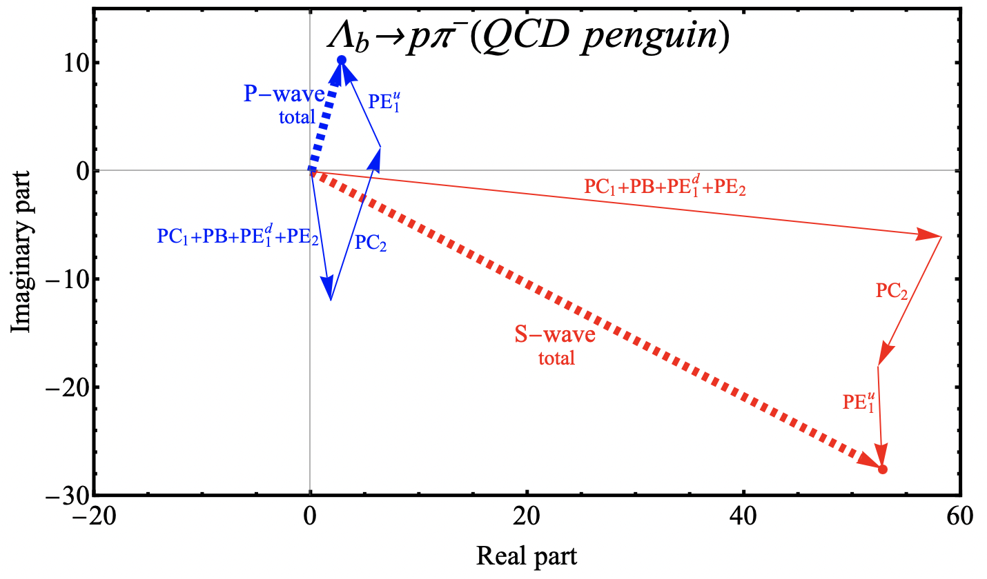
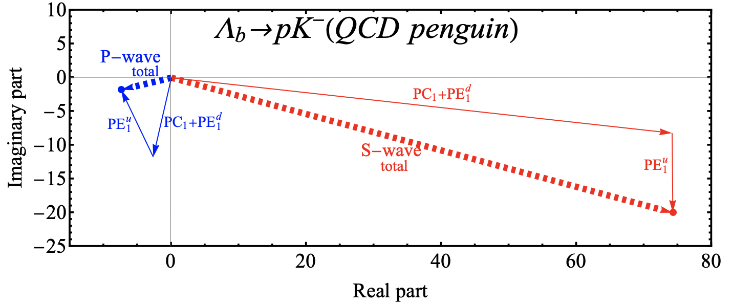
Figure 7: QCD penguin contributions from each topological diagram to the $\Lambda_{b}\to p\pi^{-}$ decay (top) and to the $\Lambda_{b}\to pK^{-}$ decay (bottom) depicted in the complex plane. The red (blue) vectors represent the $S$-wave ($P$-wave) penguin contributions.

We explain why the $PC_{2}$ and $PE_{1}^{u}$ penguins generate the dominant strong phases with opposite signs between the $S$- and $P$-wave amplitudes. For simplicity, we ignore the electroweak penguins and concentrate on the QCD penguins. The distinction between the contributions of $O_{3,4}$ and $O_{1,2}$, both being the $(V-A)\otimes(V-A)$ operators, appears only in their Wilson coefficients, such that the strong phases of the penguin amplitudes from $O_{3,4}$ are close to those of the tree amplitudes. This claim is supported by the results in Tables 11 and 12. Taking the $\Lambda_{b}\to p\pi^{-}$ decay as an example, we have $\delta^{S}=-6.26^{\circ}$ and $-10.64^{\circ}$ for the $S$-wave amplitudes from the tree and $O_{3,4}$ operators, respectively, and $\delta^{P}=-14.21^{\circ}$ and $-12.75^{\circ}$ for the $P$-wave ones from the tree and $O_{3,4}$ operators, respectively. It is also the case for $\Lambda_{b}\to pK^{-}$. The contributions from the $(V-A)\otimes(V+A)$ operators $O_{5,6}$ make the substantial strong phase differences between the penguin and tree amplitudes, which read $\delta^{S}=-40.61^{\circ}$ and $\delta^{P}=153.58^{\circ}$ for the $p\pi^{-}$ mode in Table 11, and $\delta^{S}=-18.02^{\circ}$ and $\delta^{P}=172.56^{\circ}$ for the $pK^{-}$ mode in Table 12. Figure 8, depicting the $S$- and $P$-wave amplitudes from $O_{5,6}$, justifies our analytic argument for $S_{PC_{2}}\approx-P_{PC_{2}}$ and $S_{PE_{1}^{u}}\approx-P_{PE_{1}^{u}}$.

Figure 8: $O_{5}$ and $O_{6}$ penguin contributions to the $\Lambda_{b}\to p\pi^{-}$ decay (top) and to the $\Lambda_{b}\to pK^{-}$ decay (bottom) depicted in the complex plane. The red (blue) vectors represent the $S$-wave ($P$-wave) penguin contributions.

$\Lambda_{b}\to p\pi^{-}$		$|S|$	$\delta^{S}(^{\circ})$	Re($S$)	Im($S$)	$|P|$	$\delta^{P}(^{\circ})$	Re($P$)	Im($P$)
Tree	$T$	703.07	-4.19	701.19	-51.38	1003.22	-15.33	967.54	-265.17
	$C_{2}$	29.37	154.96	-26.61	12.43	41.51	179.80	-41.51	0.14
	$E_{2}$	66.94	-145.26	-55.01	-38.14	72.58	119.94	-36.23	62.89
	$B$	10.40	112.64	-4.00	9.60	23.65	-122.56	-12.73	-19.93
	total	619.26	-6.26	615.57	-67.49	904.75	-14.21	877.08	-222.06
	$PC_{1}$	59.36	-1.62	59.34	-1.68	13.41	-81.85	1.90	-13.27
	$PC_{2}$	13.95	-114.84	-5.86	-12.66	13.89	69.92	4.77	13.05
QCD	$PE_{1}^{u}$	8.52	-93.30	-0.49	-8.51	10.23	112.10	-3.85	9.48
Penguin	$PB$	1.44	-39.65	1.11	-0.92	1.40	-162.08	-1.33	-0.43
	$PE_{1}^{d}+PE_{2}$	3.98	-101.17	-0.77	-3.90	1.35	7.65	1.34	0.18
	total	60.07	-27.41	53.33	-27.65	9.44	72.56	2.83	9.01
$O_{3,4}$	$PC_{1}$	30.41	-4.26	30.32	-2.26	43.11	-16.55	41.32	-12.28
	$PC_{2}$	1.05	179.78	-1.05	0.00	1.68	-154.82	-1.52	-0.71
	$PE_{1}^{u}$	2.18	-159.87	-2.05	-0.75	3.28	112.54	-1.26	3.03
	$PB$	0.36	103.90	-0.09	0.35	0.38	-114.38	-0.16	-0.35
	$PE_{1}^{d}+PE_{2}$	2.42	-93.34	-0.14	-2.42	1.61	86.32	0.10	1.60
	total	27.47	-10.64	27.00	-5.07	39.46	-12.75	38.49	-8.71
$O_{5,6}$	$PC_{1}$	29.02	1.15	29.02	0.58	39.44	-178.56	-39.42	-0.99
	$PC_{2}$	13.54	-110.82	-4.81	-12.66	15.13	65.45	6.29	13.76
	$PE_{1}^{u}$	7.92	-78.61	1.56	-7.76	6.95	111.88	-2.59	6.45
	$PB$	1.74	-46.52	1.20	-1.27	1.17	-176.00	-1.17	-0.08
	$PE_{1}^{d}+PE_{2}$	1.61	-113.22	-0.63	-1.48	1.89	-48.96	1.24	-1.42
	total	34.69	-40.61	26.33	-22.58	39.82	153.58	-35.66	17.72

Table 11: Results of the topological amplitudes for the $\Lambda_{b}\to p\pi^{-}$ decay in units of $10^{-9}$ without the CKM matrix elements. The QCD penguin contributions are further broken down into those from the $O_{3,4}$ and $O_{5,6}$ operators. The magnitudes and strong phases of each topological diagram are grouped in the columns of $|S|$, $\delta^{S}(^{\circ})$, $|P|$ and $\delta^{P}(^{\circ})$.

$\Lambda_{b}\to pK^{-}$		$|S|$	$\delta^{S}(^{\circ})$	Re($S$)	Im($S$)	$|P|$	$\delta^{P}(^{\circ})$	Re($P$)	Im($P$)
Tree	$T$	855.18	-3.49	853.60	-52.08	1238.05	-15.98	1190.21	-340.84
	$E_{2}$	89.06	-138.10	-66.28	-59.48	94.13	122.31	-50.31	79.56
	total	795.18	-8.06	787.31	-111.55	1169.46	-12.91	1139.90	-261.28
	$PC_{1}$	76.08	-0.81	76.07	-1.07	15.03	-106.59	-4.29	-14.40
QCD	$PE_{1}^{u}$	11.88	-88.70	0.27	-11.88	11.41	114.21	-4.68	10.41
Penguin	$PE_{1}^{d}$	7.46	-100.12	-1.31	-7.34	2.08	60.60	1.02	1.81
	total	77.72	-15.13	75.03	-20.29	8.25	-164.60	-7.95	-2.19
$O_{3,4}$	$PC_{1}$	37.18	-4.11	37.09	-2.66	53.10	-17.42	50.67	-15.89
	$PE_{1}^{u}$	2.86	-149.71	-2.47	-1.44	4.48	111.71	-1.66	4.17
	$PE_{1}^{d}$	3.00	-92.18	-0.11	-3.00	2.08	83.11	0.25	2.06
	total	35.23	-11.64	34.51	-7.11	50.20	-11.10	49.26	-9.66
$O_{5,6}$	$PC_{1}$	39.01	2.33	38.98	1.59	54.98	178.45	-54.96	1.49
	$PE_{1}^{u}$	10.79	-75.30	2.74	-10.44	6.93	115.83	-3.02	6.24
	$PE_{1}^{d}$	4.50	-105.46	-1.20	-4.34	0.81	-18.16	0.77	-0.25
	total	42.61	-18.02	40.52	-13.18	57.70	172.56	-57.21	7.47

Table 12: Same as Table 5 but for the $\Lambda_{b}\to pK^{-}$ decay.

The underlying destruction between the partial-wave CPVs in the $\Lambda_{b}\to p\pi^{-}$ decay is manifested in Figure 9, for the ratio of $|P|^{2}/|S|^{2}=1.6$ obtained in this work. It shows the dependence of the net direct CPV on partial-wave CPVs, where the red spot corresponds to our prediction. The gray narrow band specifies the partial-wave CPVs allowed by the data of the direct CPV. We can perceive how the partial-wave CPVs affect the net CPV, and how close our prediction is to the data. It is noteworthy that the $P$ wave of the decay $\Lambda_{b}\to pK^{-}$ reveals the highest partial-wave CPV, amounting to $21\%$, but with larger uncertainty compared to the $S$-wave CPV. The factorizable penguin contributions play an essential role in the $S$-wave amplitude due to the chiral factors. These contributions, being less sensitive to the proton DAs, have smaller theoretical errors. By contrast, the non-factorizable penguin contributions, dominating the $P$-wave amplitude, suffer significant uncertainties from the proton and kaon DAs, whch propagate into the $P$-wave CPVs.

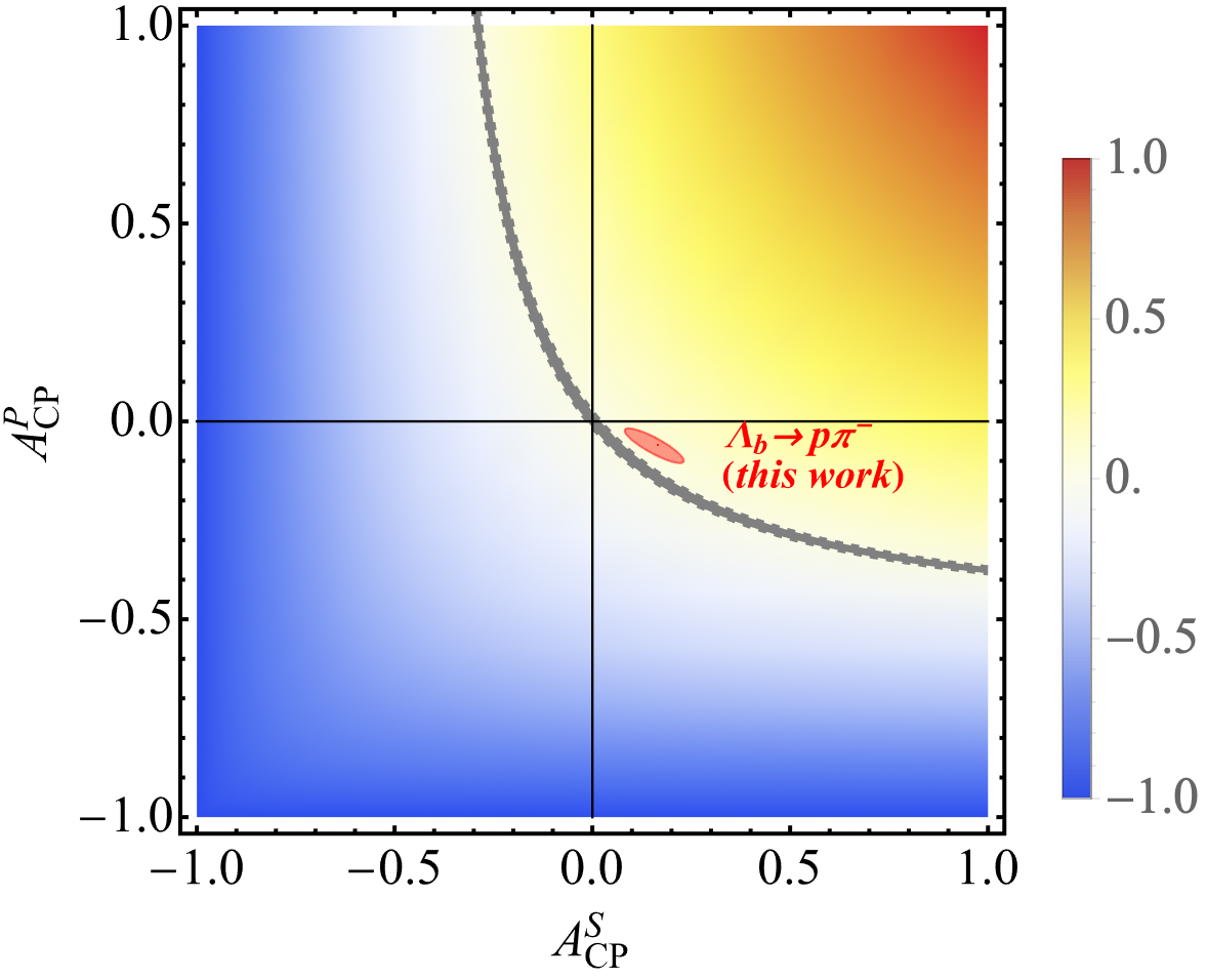
Figure 9: Dependence of the net direct CPV on partial-wave CPVs, where the red spot corresponds to our prediction. The gray narrow band specifies the partial-wave CPVs allowed by the data of the direct CPV of $\Lambda_{b}\to p\pi^{-}$.

The difference of the direct CPVs is given by

$$\begin{split}\Delta A_{CP}^{dir}(\Lambda_{b}\to pK^{-}/\pi^{-})&\equiv A_{CP}^{dir}(\Lambda_{b}\to pK^{-})-A_{CP}^{dir}(\Lambda_{b}\to p\pi^{-})\\ &=-0.11^{+0.02+0.02+0.03+0.02}_{-0.01-0.00-0.01-0.02},\end{split}$$ (61)

which slightly deviates from the measured value around $-0.01$. As mentioned in Sec. I and Ref. Han:2022srw, the threshold resummation factor for heavy baryon decays, which smooths the endpoint behavior of hard kernels and modifies tree and penguin contributions differently, has not been taken into account in the present framework. Implementing this factor may achieve more accurate predictions, improve the agreement with experimental data, and advance our understanding of the decay dynamics accordingly.

We define the decay parameters for $\Lambda_{b}\to p\pi^{-},pK^{-}$ Lee:1957qs,

$$\alpha=-\frac{2\kappa_{c}Re(S^{\ast}P)}{|S|^{2}+\kappa_{c}^{2}|P|^{2}},\quad\beta=-\frac{2\kappa_{c}Im(S^{\ast}P)}{|S|^{2}+\kappa_{c}^{2}|P|^{2}},\quad\gamma=\frac{|S|^{2}-\kappa_{c}^{2}|P|^{2}}{|S|^{2}+\kappa_{c}^{2}|P|^{2}},$$ (62)

with the coefficient $\kappa_{c}=p_{c}/(E_{p}+m_{p})=\sqrt{(E_{p}-m_{p})/(E_{p}+m_{p})}$, and their associated $CP$ asymmetries and averages,

$$\begin{split}A_{CP}^{\alpha}&=\frac{\alpha+\bar{\alpha}}{2},\quad A_{CP}^{\beta}=\frac{\beta+\bar{\beta}}{2},\quad A_{CP}^{\gamma}=\frac{\gamma-\bar{\gamma}}{2},\\ \langle\alpha\rangle&=\frac{\alpha-\bar{\alpha}}{2},\quad\langle\beta\rangle=\frac{\beta-\bar{\beta}}{2},\quad\langle\gamma\rangle=\frac{\gamma+\bar{\gamma}}{2}.\end{split}$$ (63)

The numerical outcomes for the above observables are supplied in table 10, among which the $CP$ asymmetries $A_{CP}^{\beta}$ are prominent for both the $\Lambda_{b}\to p\pi^{-},pK^{-}$ modes. However, the information on the $\Lambda_{b}$ baryon and proton polarizations is needed to measure these parameters, which are experimentally inaccessible by now.

The proton and meson masses have been retained in the kinematic variables and hard kernels in the current analysis. To quantify the impact of these supposed higher-power contributions, we neglect the proton and pion masses, and recalculate the $\Lambda_{b}\to p\pi^{-}$ decay amplitudes. The resultant branching ratio $3.65\times 10^{-6}$ and direct CPV $0.09$ in Table 13 evince that the light-hadron masses produce $15\%$ and $50\%$ effects, respectively, relative to the corresponding values in Table 10. This test manifests the importance of power corrections in heavy baryon decays.

Table 13: Same as table 5 but without the proton and meson masses in kinematics.

$\Lambda_{b}\to p\pi^{-}$	$|S|$	$\phi(S)^{\circ}$	Real($S$)	Imag($S$)	$|P|$	$\phi(P)^{\circ}$	Real($P$)	Imag($P$)
$T_{f}$	839.84	0.00	839.84	0.00	850.10	0.00	850.10	0.00
$T_{nf}$	62.83	-100.16	-11.08	-61.84	240.42	-97.09	-29.69	-238.58
$T_{f}+T_{nf}$	831.06	-4.27	828.75	-61.84	854.39	-16.21	820.41	-238.58
$C^{\prime}$	35.65	162.64	-34.02	10.64	32.99	-176.98	-32.95	-1.74
$E_{2}$	84.36	-141.20	-65.75	-52.86	51.84	128.88	-32.54	40.35
$B$	17.54	104.24	-4.32	17.00	13.74	-124.50	-7.78	-11.32
Tree	729.88	-6.85	724.66	-87.06	776.44	-15.79	747.14	-211.29
$P^{C_{1}}_{f}$	67.66	0.00	67.66	0.00	2.61	0.00	2.61	0.00
$P^{C_{1}}_{nf}$	1.83	-109.17	-0.60	-1.73	9.87	-92.94	-0.51	-9.86
$P^{C_{1}}_{f}+P^{C_{1}}_{nf}$	67.08	-1.48	67.06	-1.73	10.08	-77.93	2.11	-9.86
$P^{C_{2}}$	17.24	-116.06	-7.57	-15.49	13.63	67.60	5.19	12.60
$P^{E_{1}^{u}}$	11.22	-90.55	-0.11	-11.22	7.06	112.49	-2.70	6.52
$P^{B}$	1.30	-42.87	0.96	-0.89	1.40	-170.77	-1.38	-0.22
$P^{E_{1}^{d}}+P^{E_{2}}$	4.68	-101.65	-0.95	-4.59	1.62	-12.75	1.58	-0.36
Penguin	68.39	-29.72	59.39	-33.91	9.92	61.02	4.81	8.68

III.2 Quasi-two-body $\Lambda_{b}\to pV$ decays

The $\Lambda_{b}\to pV$ decay amplitudes for longitudinally and transversely polarized vector mesons $V=\rho^{-},K^{\ast-}$ are decomposed into

$$\begin{split}\mathcal{A}^{L}=&\bar{u}_{p}\Big{(}A_{1}^{L}\gamma^{\mu}\gamma_{5}+A_{2}^{L}\frac{p_{p}^{\mu}}{m_{\Lambda_{b}}}\gamma_{5}+B_{1}^{L}\gamma^{\mu}+B_{2}^{L}\frac{p_{p}^{\mu}}{m_{\Lambda_{b}}}\Big{)}u_{\Lambda_{b}}\epsilon_{L\mu}^{\ast},\\ \mathcal{A}^{T}=&\bar{u}_{p}(A_{1}^{T}\gamma^{\mu}\gamma_{5}+B_{1}^{T}\gamma^{\mu})u_{\Lambda_{b}}\epsilon_{T\mu}^{\ast},\end{split}$$ (64)

with the longitudinal (transverse) polarization vector $\epsilon_{L(T)}$. The polarization amplitudes $A_{1}^{L,T}$, $A_{2}^{L}$, $B_{1}^{L,T}$ and $B_{2}^{L}$ form the partial-wave amplitudes

$$\begin{split}S^{L}=&-A_{1}^{L},\\ S^{T}=&-A_{1}^{T},\\ P_{1}=&-\frac{p_{c}}{E_{V}}\left(\frac{m_{\Lambda_{b}}+m_{p}}{E_{p}+m_{p}}B_{1}^{L}+B_{2}^{L}\right),\\ P_{2}=&\frac{p_{c}}{E_{p}+m_{p}}B_{1}^{T},\\ D=&-\frac{p_{c}^{2}}{E_{V}(E_{p}+m_{p})}\left(A_{1}^{L}-A_{2}^{L}\right),\end{split}$$ (65)

and the helicity amplitudes

$$\begin{split}H_{\frac{1}{2},1}=&-\sqrt{2}M_{+}A_{1}^{T}-\sqrt{2}M_{-}B_{1}^{T},\\ H_{-\frac{1}{2},-1}=&\sqrt{2}M_{+}A_{1}^{T}-\sqrt{2}M_{-}B_{1}^{T},\\ H_{\frac{1}{2},0}=&\left(M_{+}(m_{\Lambda_{b}}-m_{p})A_{1}^{L}-M_{-}p_{c}A_{2}^{L}+M_{-}(m_{\Lambda_{b}}+m_{p})B_{1}^{L}+M_{+}p_{c}B_{2}^{L}\right)/m_{V},\\ H_{-\frac{1}{2},0}=&\left(-M_{+}(m_{\Lambda_{b}}-m_{p})A_{1}^{L}+M_{-}p_{c}A_{2}^{L}+M_{-}(m_{\Lambda_{b}}+m_{p})B_{1}^{L}+M_{+}p_{c}B_{2}^{L}\right)/m_{V},\end{split}$$ (66)

with the vector meson energy $E_{V}$.

Given the numerical results in Appendix LABEL:app:appendix-numerical-results for the above amplitudes, the $\Lambda_{b}\to pV$ decay width is derived via

$$\begin{split}\Gamma=&\frac{p_{c}}{4\pi}\frac{E_{p}+m_{p}}{m_{\Lambda_{b}}}\left\{2(|S^{T}|^{2}+|P_{2}|^{2})+\frac{E_{V}^{2}}{m_{V}^{2}}(|S^{L}+D|^{2}+|P_{1}|^{2})\right\}\\ =&\frac{p_{c}}{16\pi m_{\Lambda_{b}}^{2}}(|H_{1/2,1}|^{2}+|H_{-1/2,-1}|^{2}+|H_{1/2,0}|^{2}+|H_{-1/2,0}|^{2}).\end{split}$$ (67)

The associated partial-wave CPVs are defined as in Eq. (58), in terms of which the direct CPV is decomposed Han:2024kgz,

$$A_{CP}^{dir}\approx\kappa_{S^{T}}A_{CP}^{S^{T}}+\kappa_{P_{1}}A_{CP}^{P_{1}}+\kappa_{P_{2}}A_{CP}^{P_{2}}+\kappa_{D+S^{L}}A_{CP}^{D+S^{L}},$$ (68)

with the weights

$$\begin{split}\kappa_{S^{T}}=&\frac{2|S^{T}|^{2}}{\Pi},\quad\kappa_{P_{1}}=\frac{E_{V}^{2}|P_{1}|^{2}}{m_{V}^{2}\Pi},\\ \kappa_{P_{2}}=&\frac{2|P_{2}|^{2}}{\Pi},\quad\kappa_{D+S^{L}}=\frac{E_{V}^{2}|D+S^{L}|^{2}}{m_{V}^{2}\Pi},\\ \Pi\equiv&2|S^{T}|^{2}+2|P_{2}|^{2}+E_{V}^{2}/m_{V}^{2}|D+S^{L}|^{2}+E_{V}^{2}/m_{V}^{2}|P_{1}|^{2}.\end{split}$$ (69)

The predictions for the branching ratios and CPVs of the $\Lambda_{b}\to p\rho^{-},pK^{\ast-}$ decays are collected in Table 14. Unlike $\Lambda_{b}\to p\pi^{-},pK^{-}$, whose branching ratios are of the same order, the $\Lambda_{b}\to p\rho^{-}$ branching ratio is greater than the $pK^{\ast-}$ one by a factor of $3$. The operators $O_{5,6,7,8}$ do not contribute to the factorizable penguin topologies as shown in Eq. (36). Hence, the enhancement of the penguin amplitudes by the chiral factor in Eq. (50) is absent in the$\Lambda_{b}\to pK^{\ast-}$ decay.

It is found that the $D+S^{L}$ and $P_{1}$ components dominate the direct CPVs because of the enhancement factor $E_{V}/m_{V}$. The partial-wave CPVs of the $\Lambda_{b}\to pV$ decays also exceed $10\%$; the $P_{2}\text{-wave}$ CPVs of $\Lambda_{b}\to p\rho^{-}$ reaches $17\%$; the $(D+S^{L})\text{-wave}$ CPV of $\Lambda_{b}\to pK^{*-}$ is even as large as $27\%$. However, the direct CPVs of these modes are all minor for the similar reasons. The relative sign of the partial-wave amplitudes in the $\Lambda_{b}\to pK^{*-}$ decay can be argued in the same manner. Their tiny direct CPVs trace back to the destruction between the major $(D+S^{L})$- and $P_{1}\text{-wave}$ CPVs, like the $\Lambda_{b}\to p\pi^{-}$ case. For the $\Lambda_{b}\to p\rho^{-}$ decay, the two dominant partial-wave CPVs are small, leading to a negligible direct CPV.

Table 14: Same as Table 10 but for the $\Lambda_{b}\to p\rho^{-},pK^{\ast-}$ decays.

	$Br(\times 10^{-6})$	$A_{CP}^{dir}$	$A_{CP}^{S^{T}}(\kappa_{S^{T}})$
$\Lambda_{b}\to p\rho^{-}$	$9.66^{+6.23+3.23+0.21+1.89}_{-3.50-3.03-1.20-0.75}$	$0.03^{+0.02+0.01+0.00+0.02}_{-0.02-0.03-0.03-0.02}$	$0.01^{+0.00+0.00+0.00+0.00}_{-0.01-0.02-0.02-0.02}(7\%)$
$\Lambda_{b}\to pK^{\ast-}$	$2.83^{+1.77+0.46+0.37+0.63}_{-1.29-1.23-0.53-0.66}$	$-0.05^{+0.04+0.07+0.01+0.05}_{-0.11-0.07-0.06-0.08}$	$-0.15^{+0.06+0.09+0.02+0.05}_{-0.00-0.04-0.05-0.00}(6\%)$
	$A_{CP}^{S^{L}+D}(\kappa_{S^{L}+D})$	$A_{CP}^{P_{1}}(\kappa_{P_{1}})$	$A_{CP}^{P_{2}}(\kappa_{P_{2}})$
$\Lambda_{b}\to p\rho^{-}$	$0.02^{+0.03+0.04+0.02+0.05}_{-0.02-0.02-0.00-0.00}(44\%)$	$0.03^{+0.04+0.00+0.00+0.00}_{-0.05-0.04-0.10-0.05}(45\%)$	$0.17^{+0.00+0.00+0.01+0.03}_{-0.02-0.03-0.03-0.04}(4\%)$
$\Lambda_{b}\to pK^{\ast-}$	$0.27^{+0.02+0.06+0.05+0.03}_{-0.17-0.11-0.02-0.18}(33\%)$	$-0.23^{+0.05+0.07+0.02+0.05}_{-0.11-0.11-0.09-0.03}(55\%)$	$-0.14^{+0.01+0.00+0.02+0.01}_{-0.04-0.09-0.02-0.03}(6\%)$
	$\alpha$	$A_{CP}^{\alpha}$	$\langle\alpha\rangle$
$\Lambda_{b}\to p\rho^{-}$	$-0.83^{+0.02+0.01+0.00+0.00}_{-0.02-0.05-0.04-0.01}$	$-0.01^{+0.01+0.01+0.01+0.00}_{-0.00-0.00-0.01-0.00}$	$-0.83^{+0.01+0.01+0.01+0.00}_{-0.02-0.05-0.04-0.01}$
$\Lambda_{b}\to pK^{\ast-}$	$-1.00^{+0.01+0.01+0.00+0.01}_{-0.00-0.00-0.00-0.00}$	$-0.00^{+0.00+0.00+0.00+0.00}_{-0.00-0.00-0.00-0.00}$	$-1.00^{+0.00+0.01+0.00+0.00}_{-0.00-0.00-0.00-0.00}$
	$\beta$	$A_{CP}^{\beta}$	$\langle\beta\rangle$
$\Lambda_{b}\to p\rho^{-}$	$-0.98^{+0.05+0.07+0.05+0.06}_{-0.00-0.00-0.00-0.00}$	$0.00^{+0.01+0.02+0.01+0.02}_{-0.00-0.00-0.00-0.00}$	$-0.99^{+0.04+0.05+0.04+0.04}_{-0.00-0.00-0.00-0.00}$
$\Lambda_{b}\to pK^{\ast-}$	$-0.90^{+0.07+0.17+0.11+0.00}_{-0.03-0.03-0.00-0.03}$	$-0.02^{+0.04+0.06+0.04+0.01}_{-0.00-0.04-0.00-0.00}$	$-0.88^{+0.06+0.11+0.08+0.00}_{-0.03-0.06-0.00-0.04}$
	$\gamma$	$A_{CP}^{\gamma}$	$\langle\gamma\rangle$
$\Lambda_{b}\to p\rho^{-}$	$-0.11^{+0.01+0.01+0.01+0.01}_{-0.01-0.01-0.02-0.00}$	$-0.01^{+0.00+0.00+0.00+0.00}_{-0.00-0.00-0.00-0.00}$	$-0.10^{+0.01+0.01+0.01+0.00}_{-0.01-0.01-0.02-0.00}$
$\Lambda_{b}\to pK^{\ast-}$	$-0.12^{+0.01+0.00+0.02+0.00}_{-0.06-0.05-0.03-0.05}$	$0.02^{+0.01+0.03+0.01+0.01}_{-0.02-0.02-0.01-0.01}$	$-0.14^{+0.01+0.01+0.02+0.00}_{-0.04-0.07-0.04-0.04}$
	$\Lambda$	$A_{CP}^{\Lambda}$	$\langle\Lambda\rangle$
$\Lambda_{b}\to p\rho^{-}$	$-0.96^{+0.05+0.06+0.04+0.05}_{-0.00-0.00-0.00-0.00}$	$0.00^{+0.01+0.02+0.01+0.02}_{-0.00-0.00-0.00-0.00}$	$-0.97^{+0.04+0.04+0.03+0.04}_{-0.00-0.00-0.00-0.00}$
$\Lambda_{b}\to pK^{\ast-}$	$-0.91^{+0.06+0.15+0.09+0.00}_{-0.02-0.02-0.00-0.03}$	$-0.01^{+0.03+0.06+0.03+0.01}_{-0.00-0.03-0.00-0.00}$	$-0.90^{+0.05+0.09+0.07+0.00}_{-0.03-0.05-0.01-0.03}$
	$\mathcal{J}$	$A_{CP}^{\mathcal{J}}$	$\langle\mathcal{J}\rangle$
$\Lambda_{b}\to p\rho^{-}$	$1.66^{+0.04+0.04+0.02+0.02}_{-0.03-0.03-0.05-0.00}$	$-0.01^{+0.01+0.01+0.01+0.00}_{-0.01-0.01-0.01-0.00}$	$1.67^{+0.03+0.04+0.02+0.02}_{-0.05-0.03-0.05-0.00}$
$\Lambda_{b}\to pK^{\ast-}$	$1.67^{+0.02+0.00+0.04+0.00}_{-0.14-0.12-0.08-0.12}$	$0.04^{+0.02+0.05+0.02+0.01}_{-0.06-0.04-0.02-0.03}$	$1.63^{+0.01+0.03+0.04+0.00}_{-0.08-0.15-0.09-0.09}$

The decay asymmetry parameters are expressed, in terms of the helicity amplitudes, as

$$\begin{split}\alpha&=\frac{|H_{1/2,1}|^{2}-|H_{-1/2,-1}|^{2}}{|H_{1/2,1}|^{2}+|H_{-1/2,-1}|^{2}},\quad\beta=\frac{|H_{1/2,0}|^{2}-|H_{-1/2,0}|^{2}}{|H_{1/2,0}|^{2}+|H_{-1/2,0}|^{2}},\quad\gamma=\frac{|H_{1/2,1}|^{2}-|H_{-1/2,-1}|^{2}}{|H_{1/2,0}|^{2}+|H_{-1/2,0}|^{2}},\\ \Lambda&=\frac{|H_{1/2,1}|^{2}-|H_{-1/2,-1}|^{2}+|H_{1/2,0}|^{2}-|H_{-1/2,0}|^{2}}{|H_{1/2,1}|^{2}+|H_{-1/2,-1}|^{2}+|H_{1/2,0}|^{2}+|H_{-1/2,0}|^{2}},\end{split}$$ (70)

which satisfy $\Lambda=(\beta+\alpha\gamma)/(1+\gamma)$. The associated CPVs and averages are defined as in Eq. (63) and by

$$\begin{split}A_{CP}^{\Lambda}=\frac{\Lambda+\bar{\Lambda}}{2},\quad\langle\Lambda\rangle=\frac{\Lambda-\bar{\Lambda}}{2}.\end{split}$$ (71)

The results for the above quantities in Table 14 clearly imply that the CPVs of the decay asymmetry parameters are all consistent with zero.

Since a vector meson decays strongly with a finite width, what we worked on are actually the three-body decays $\Lambda_{b}\to p(\rho^{-}\to)\pi^{-}\pi^{0},p(K^{\ast-}\to)K^{-}\pi^{0}$. Motivated by the sizable partial-wave CPVs, we investigate the potential observables for identifying CPVs involved in the angle distributions for three-body decays. The angle distribution of $\Lambda_{b}\to pV\to ph_{1}h_{2}$ in Fig. 10 is formulated as

$$\begin{split}\frac{d\Gamma}{d\cos\theta}&\propto|H_{\frac{1}{2},0}|^{2}+|H_{-\frac{1}{2},0}|^{2}+|H_{-\frac{1}{2},-1}|^{2}+|H_{\frac{1}{2},1}|^{2}\\ &\hskip 14.22636pt+(2|H_{\frac{1}{2},0}|^{2}+2|H_{-\frac{1}{2},0}|^{2}-|H_{-\frac{1}{2},-1}|^{2}-|H_{\frac{1}{2},1}|^{2})P_{2}\\ &\propto 1+\mathcal{J}\cdot P_{2},\end{split}$$ (72)

where the observable

$$\mathcal{J}\equiv\frac{2|H_{\frac{1}{2},0}|^{2}+2|H_{-\frac{1}{2},0}|^{2}-|H_{-\frac{1}{2},-1}|^{2}-|H_{\frac{1}{2},1}|^{2}}{|H_{\frac{1}{2},0}|^{2}+|H_{-\frac{1}{2},0}|^{2}+|H_{-\frac{1}{2},-1}|^{2}+|H_{\frac{1}{2},1}|^{2}},$$ (73)

with the Legendre polynomial $P_{2}=(3\cos^{2}\theta-1)/2$ can be extracted from data fitting. The CPV and average for $\mathcal{J}$ are written as

$$A_{CP}^{\mathcal{J}}=\frac{\mathcal{J}-\bar{\mathcal{J}}}{2},\qquad\langle\mathcal{J}\rangle=\frac{\mathcal{J}+\bar{\mathcal{J}}}{2},$$ (74)

whose predictions are listed in Table 14. Unfortunately, the CPVs $A_{CP}^{\mathcal{J}}$ in the $\Lambda_{b}\to p\rho^{-},pK^{\ast-}$ decays are too tiny to search for experimentally.

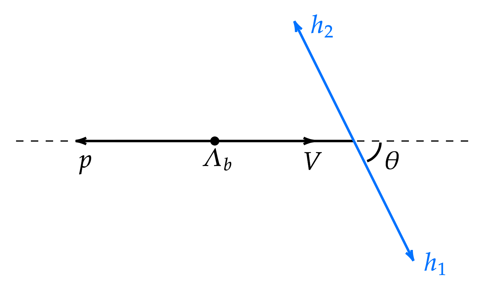
Figure 10: Configuration of the $\Lambda_{b}\to pV\to ph_{1}h_{2}$ decay, where $\theta$ is the angle between $h_{1}$ in the $V$ rest frame and the $V$ momentum in the $\Lambda_{b}$ rest frame.

III.3 Quasi-two-body $\Lambda_{b}\to pA$ decays

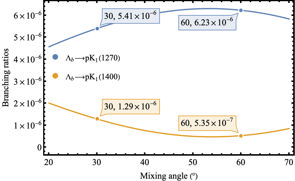
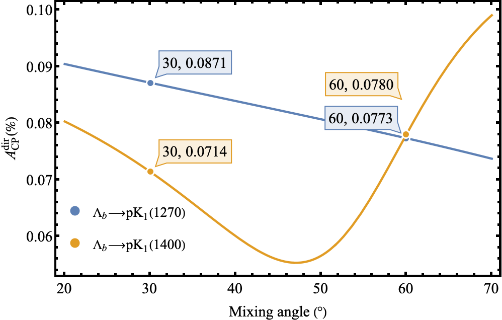
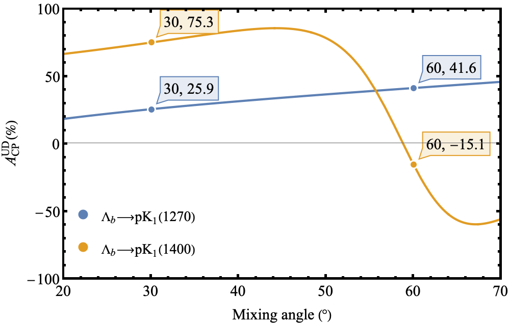
Figure 11: (upper-left) Dependencies of the $\Lambda_{b}\to pK_{1}$ branching ratios on the mixing angle $\theta_{K}$; (upper-right) same as the up-left panel but for the direct CPVs; (bottom) same as the up-left panel but for the CPVs in the up-down asymmetry.

The decays $\Lambda_{b}\to pA$, with $A$ denoting the axial-vector mesons $a^{-}_{1}(1260),K^{-}_{1}(1270),K^{-}_{1}(1400)$, share the same amplitude parametrization and observables as $\Lambda_{b}\to pV$ in the previous subsection. Because the $K_{1}(1270)$-$K_{1}(1400)$ mixing angle $\theta_{K}$ is not yet well determined Shi:2023kiy, we take the typical values $\theta_{K}=30^{\circ}$ and $60^{\circ}$ for illustration. It is seen that most of our predictions in Table 15 are insensitive to $\theta_{K}$. The predicted $\Lambda_{b}\to pa^{-}_{1}(1260)$ and $\Lambda_{b}\to pK^{-}_{1}(1270,1400)$ branching ratios are of the order $10^{-6}$, which can be verified experimentally. The partial-wave CPVs of the $\Lambda_{b}\to pa^{-}_{1}(1260),pK^{-}_{1}(1270),pK^{-}_{1}(1400)$ decays are significant, exceeding $50\%$. The opposite signs between the partial-wave CPVs turn in the minor direct CPV of $\Lambda_{b}\to pa_{1}^{-}(1260)$. The direct CPVs of $\Lambda_{b}\to pK_{1}(1270)^{-},pK_{1}(1400)^{-}$ can deviate from zero, both of which are above $+5\%$ in the range $20^{\circ}\sim 70^{\circ}$ of the mixing angle as plotted in Fig. 11.

Table 15: Same as Table 10 but for the $\Lambda_{b}\to pA$ decays.

	$Br(\times 10^{-6})$	$A_{CP}^{dir}$	$A_{CP}^{S^{T}}(\kappa_{S^{T}})$
$\Lambda_{b}\to pa_{1}^{-}(1260)$	$11.06^{+8.21+3.88+0.91+1.73}_{-4.30-3.32-0.46-0.06}$	$-0.01^{+0.01+0.03+0.02+0.03}_{-0.00-0.01-0.02-0.00}$	$-0.22^{+0.04+0.07+0.05+0.04}_{-0.03-0.07-0.07-0.01}(6\%)$
$\Lambda_{b}\to pK_{1}^{-}(1270)(30^{\circ})$	$5.48^{+3.63+1.94+0.27+2.49}_{-1.87-1.55-0.31-1.11}$	$0.09^{+0.03+0.07+0.03+0.01}_{-0.04-0.02-0.02-0.00}$	$0.34^{+0.00+0.01+0.01+0.00}_{-0.02-0.03-0.01-0.05}(8\%)$
$\Lambda_{b}\to pK_{1}^{-}(1400)(30^{\circ})$	$1.25^{+0.59+0.33+0.13+0.64}_{-0.39-0.19-0.19-0.31}$	$0.06^{+0.03+0.05+0.03+0.00}_{-0.03-0.09-0.04-0.01}$	$0.71^{+0.05+0.06+0.03+0.03}_{-0.02-0.16-0.04-0.13}(13\%)$
$\Lambda_{b}\to pK_{1}^{-}(1270)(60^{\circ})$	$6.28^{+3.97+1.93+0.18+2.79}_{-2.13-1.51-0.41-1.32}$	$0.07^{+0.01+0.03+0.03+0.01}_{-0.04-0.04-0.03-0.00}$	$0.46^{+0.00+0.00+0.02+0.01}_{-0.02-0.04-0.02-0.07}(9\%)$
$\Lambda_{b}\to pK_{1}^{-}(1400)(60^{\circ})$	$0.53^{+0.33+0.38+0.09+0.36}_{-0.16-0.19-0.22-0.13}$	$0.08^{+0.11+0.09+0.12+0.00}_{-0.08-0.11-0.04-0.03}$	$0.07^{+0.00+0.41+0.08+0.22}_{-0.12-0.09-0.15-0.10}(3\%)$
	$A_{CP}^{S^{L}+D}(\kappa_{S^{L}+D})$	$A_{CP}^{P_{1}}(\kappa_{P_{1}})$	$A_{CP}^{P_{2}}(\kappa_{P_{2}})$
$\Lambda_{b}\to pa_{1}^{-}(1260)$	$-0.11^{+0.02+0.01+0.02+0.02}_{-0.00-0.01-0.07-0.03}(46\%)$	$0.18^{+0.03+0.02+0.04+0.09}_{-0.03-0.02-0.03-0.04}(40\%)$	$-0.24^{+0.01+0.05+0.04+0.03}_{-0.02-0.09-0.06-0.06}(8\%)$
$\Lambda_{b}\to pK_{1}^{-}(1270)(30^{\circ})$	$-0.11^{+0.01+0.08+0.08+0.03}_{-0.04-0.06-0.03-0.00}(42\%)$	$0.19^{+0.10+0.13+0.05+0.02}_{-0.06-0.09-0.11-0.01}(42\%)$	$0.33^{+0.00+0.04+0.02+0.00}_{-0.02-0.03-0.02-0.03}(8\%)$
$\Lambda_{b}\to pK_{1}^{-}(1400)(30^{\circ})$	$0.81^{+0.09+0.17+0.07+0.04}_{-0.12-0.14-0.11-0.00}(17\%)$	$-0.41^{+0.04+0.05+0.08+0.03}_{-0.07-0.05-0.11-0.04}(60\%)$	$0.78^{+0.04+0.11+0.09+0.05}_{-0.06-0.20-0.04-0.10}(10\%)$
$\Lambda_{b}\to pK_{1}^{-}(1270)(60^{\circ})$	$0.06^{+0.01+0.08+0.07+0.03}_{-0.03-0.07-0.04-0.00}(37\%)$	$-0.07^{+0.05+0.06+0.04+0.01}_{-0.06-0.05-0.05-0.02}(45\%)$	$0.46^{+0.00+0.04+0.04+0.02}_{-0.01-0.03-0.02-0.06}(9\%)$
$\Lambda_{b}\to pK_{1}^{-}(1400)(60^{\circ})$	$-0.82^{+0.14+0.19+0.12+0.21}_{-0.07-0.09-0.07-0.02}(30\%)$	$0.52^{+0.06+0.12+0.37+0.00}_{-0.01-0.14-0.03-0.07}(64\%)$	$-0.28^{+0.27+0.04+0.03+0.03}_{-0.07-0.36-0.25-0.16}(3\%)$
	$\alpha$	$A_{CP}^{\alpha}$	$\langle\alpha\rangle$
$\Lambda_{b}\to pa_{1}^{-}(1260)$	$-0.86^{+0.01+0.02+0.03+0.00}_{-0.03-0.05-0.05-0.03}$	$0.02^{+0.00+0.01+0.01+0.00}_{-0.00-0.01-0.00-0.00}$	$-0.88^{+0.01+0.02+0.04+0.00}_{-0.03-0.04-0.05-0.02}$
$\Lambda_{b}\to pK_{1}^{-}(1270)(30^{\circ})$	$-1.00^{+0.00+0.00+0.00+0.00}_{-0.00-0.00-0.00-0.00}$	$0.00^{+0.00+0.00+0.00+0.00}_{-0.00-0.00-0.00-0.00}$	$-1.00^{+0.00+0.00+0.00+0.00}_{-0.00-0.00-0.00-0.00}$
$\Lambda_{b}\to pK_{1}^{-}(1400)(30^{\circ})$	$-1.00^{+0.00+0.01+0.01+0.00}_{-0.00-0.00-0.00-0.00}$	$-0.01^{+0.01+0.01+0.01+0.00}_{-0.00-0.04-0.06-0.02}$	$-0.98^{+0.01+0.05+0.07+0.02}_{-0.01-0.01-0.01-0.00}$
$\Lambda_{b}\to pK_{1}^{-}(1270)(60^{\circ})$	$-1.00^{+0.00+0.00+0.00+0.00}_{-0.00-0.00-0.00-0.00}$	$0.00^{+0.00+0.00+0.00+0.00}_{-0.00-0.00-0.00-0.00}$	$-1.00^{+0.00+0.00+0.01+0.00}_{-0.00-0.00-0.00-0.00}$
$\Lambda_{b}\to pK_{1}^{-}(1400)(60^{\circ})$	$-0.96^{+0.01+0.10+0.10+0.04}_{-0.03-0.03-0.03-0.00}$	$-0.00^{+0.01+0.01+0.02+0.00}_{-0.00-0.02-0.01-0.01}$	$-0.96^{+0.00+0.09+0.08+0.05}_{-0.04-0.03-0.03-0.00}$
	$\beta$	$A_{CP}^{\beta}$	$\langle\beta\rangle$
$\Lambda_{b}\to pa_{1}^{-}(1260)$	$-0.98^{+0.01+0.02+0.01+0.03}_{-0.01-0.02-0.01-0.00}$	$-0.01^{+0.01+0.01+0.01+0.01}_{-0.01-0.01-0.01-0.00}$	$-0.97^{+0.01+0.01+0.02+0.02}_{-0.01-0.01-0.02-0.01}$
$\Lambda_{b}\to pK_{1}^{-}(1270)(30^{\circ})$	$-0.99^{+0.00+0.03+0.03+0.00}_{-0.00-0.01-0.00-0.01}$	$0.00^{+0.00+0.02+0.00+0.00}_{-0.01-0.02-0.00-0.01}$	$-0.98^{+0.01+0.02+0.03+0.00}_{-0.00-0.00-0.00-0.00}$
$\Lambda_{b}\to pK_{1}^{-}(1400)(30^{\circ})$	$-0.15^{+0.28+0.17+0.13+0.25}_{-0.10-0.10-0.16-0.09}$	$0.07^{+0.04+0.07+0.08+0.03}_{-0.01-0.02-0.04-0.03}$	$-0.22^{+0.24+0.17+0.10+0.22}_{-0.10-0.11-0.15-0.06}$
$\Lambda_{b}\to pK_{1}^{-}(1270)(60^{\circ})$	$-0.95^{+0.04+0.06+0.04+0.01}_{-0.03-0.03-0.02-0.01}$	$0.00^{+0.00+0.01+0.01+0.00}_{-0.01-0.01-0.01-0.00}$	$-0.95^{+0.04+0.05+0.04+0.02}_{-0.02-0.03-0.01-0.01}$
$\Lambda_{b}\to pK_{1}^{-}(1400)(60^{\circ})$	$-0.01^{+0.01+0.07+0.10+0.09}_{-0.06-0.17-0.28-0.18}$	$-0.26^{+0.09+0.09+0.03+0.03}_{-0.01-0.05-0.12-0.09}$	$0.25^{+0.12+0.07+0.11+0.06}_{-0.15-0.16-0.18-0.09}$
	$\gamma$	$A_{CP}^{\gamma}$	$\langle\gamma\rangle$
$\Lambda_{b}\to pa_{1}^{-}(1260)$	$-0.10^{+0.01+0.01+0.02+0.00}_{-0.01-0.02-0.02-0.01}$	$0.04^{+0.01+0.02+0.01+0.01}_{-0.01-0.01-0.00-0.00}$	$-0.14^{+0.01+0.01+0.02+0.00}_{-0.02-0.03-0.01-0.01}$
$\Lambda_{b}\to pK_{1}^{-}(1270)(30^{\circ})$	$-0.24^{+0.04+0.03+0.02+0.01}_{-0.03-0.03-0.02-0.04}$	$-0.06^{+0.01+0.02+0.01+0.00}_{-0.01-0.01-0.01-0.00}$	$-0.18^{+0.03+0.02+0.01+0.00}_{-0.02-0.02-0.01-0.04}$
$\Lambda_{b}\to pK_{1}^{-}(1400)(30^{\circ})$	$-0.61^{+0.15+0.23+0.13+0.00}_{-0.16-0.26-0.19-0.09}$	$-0.27^{+0.06+0.09+0.06+0.00}_{-0.07-0.08-0.09-0.05}$	$-0.34^{+0.08+0.14+0.07+0.00}_{-0.09-0.19-0.11-0.04}$
$\Lambda_{b}\to pK_{1}^{-}(1270)(60^{\circ})$	$-0.32^{+0.06+0.06+0.02+0.00}_{-0.04-0.06-0.03-0.06}$	$-0.10^{+0.02+0.03+0.01+0.00}_{-0.02-0.01-0.01-0.01}$	$-0.22^{+0.04+0.04+0.01+0.00}_{-0.02-0.05-0.02-0.05}$
$\Lambda_{b}\to pK_{1}^{-}(1400)(60^{\circ})$	$-0.05^{+0.02+0.02+0.01+0.02}_{-0.01-0.06-0.03-0.01}$	$0.01^{+0.01+0.03+0.03+0.00}_{-0.01-0.01-0.00-0.01}$	$-0.06^{+0.01+0.01+0.01+0.02}_{-0.01-0.08-0.06-0.01}$
	$\Lambda$	$A_{CP}^{\Lambda}$	$\langle\Lambda\rangle$
$\Lambda_{b}\to pa_{1}^{-}(1260)$	$-0.97^{+0.00+0.02+0.01+0.03}_{-0.01-0.02-0.01-0.00}$	$-0.01^{+0.01+0.01+0.01+0.01}_{-0.01-0.01-0.01-0.00}$	$-0.96^{+0.01+0.01+0.02+0.02}_{-0.01-0.01-0.02-0.01}$
$\Lambda_{b}\to pK_{1}^{-}(1270)(30^{\circ})$	$-0.99^{+0.00+0.02+0.03+0.00}_{-0.00-0.01-0.00-0.01}$	$0.00^{+0.00+0.02+0.00+0.00}_{-0.01-0.02-0.00-0.01}$	$-0.99^{+0.01+0.01+0.02+0.00}_{-0.00-0.00-0.00-0.00}$
$\Lambda_{b}\to pK_{1}^{-}(1400)(30^{\circ})$	$-0.47^{+0.14+0.16+0.06+0.14}_{-0.02-0.11-0.14-0.08}$	$-0.07^{+0.06+0.08+0.05+0.00}_{-0.02-0.04-0.04-0.03}$	$-0.40^{+0.17+0.09+0.08+0.15}_{-0.06-0.11-0.13-0.05}$
$\Lambda_{b}\to pK_{1}^{-}(1270)(60^{\circ})$	$-0.96^{+0.03+0.05+0.03+0.01}_{-0.03-0.02-0.01-0.01}$	$0.00^{+0.00+0.01+0.00+0.00}_{-0.01-0.00-0.01-0.00}$	$-0.96^{+0.03+0.04+0.04+0.01}_{-0.02-0.02-0.01-0.01}$
$\Lambda_{b}\to pK_{1}^{-}(1400)(60^{\circ})$	$-0.06^{+0.10+0.08+0.10+0.11}_{-0.07-0.17-0.29-0.18}$	$-0.23^{+0.09+0.08+0.03+0.02}_{-0.01-0.01-0.08-0.08}$	$0.18^{+0.11+0.07+0.11+0.09}_{-0.14-0.17-0.22-0.10}$
	$a_{UD}$	$A_{CP}^{UD}$
$\Lambda_{b}\to pa_{1}^{-}(1260)$	$-0.09^{+0.00+0.01+0.02+0.00}_{-0.01-0.01-0.01-0.01}$	$-0.24^{+0.03+0.05+0.05+0.03}_{-0.03-0.09-0.06-0.06}$
$\Lambda_{b}\to pK_{1}^{-}(1270)(30^{\circ})$	$-0.19^{+0.03+0.02+0.01+0.01}_{-0.02-0.02-0.01-0.02}$	$0.26^{+0.02+0.03+0.01+0.00}_{-0.03-0.08-0.04-0.04}$
$\Lambda_{b}\to pK_{1}^{-}(1400)(30^{\circ})$	$-0.38^{+0.06+0.10+0.05+0.00}_{-0.06-0.09-0.07-0.03}$	$0.72^{+0.05+0.13+0.07+0.05}_{-0.05-0.23-0.03-0.12}$
$\Lambda_{b}\to pK_{1}^{-}(1270)(60^{\circ})$	$-0.24^{+0.04+0.04+0.01+0.00}_{-0.02-0.03-0.02-0.03}$	$0.40^{+0.02+0.03+0.02+0.01}_{-0.01-0.04-0.03-0.07}$
$\Lambda_{b}\to pK_{1}^{-}(1400)(60^{\circ})$	$-0.04^{+0.02+0.02+0.01+0.02}_{-0.01-0.05-0.03-0.01}$	$-0.19^{+0.12+0.14+0.00+0.06}_{-0.18-0.19-0.20-0.00}$

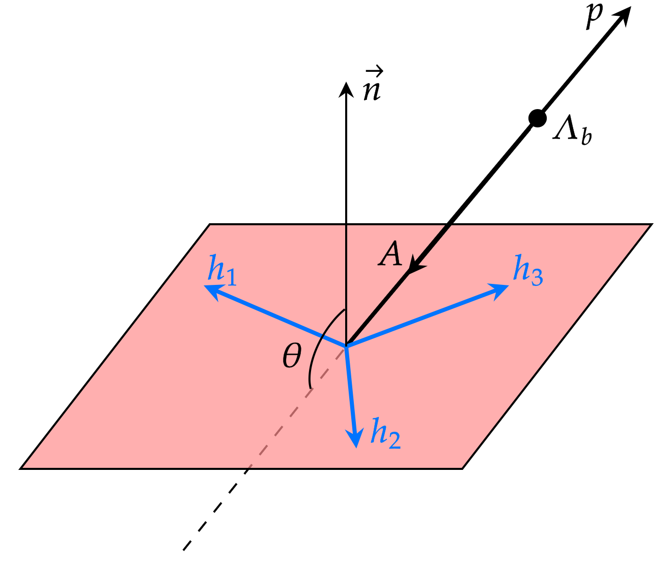
Figure 12: Configuration of the $\Lambda_{b}\to pA\to ph_{1}h_{2}h_{3}$ decay, where $\theta$ is the angle between the normal of the $A\to h_{1}h_{2}h_{3}$ decay plane and the $A$ meson momentum in the $\Lambda_{b}$ rest frame.

The $\Lambda_{b}\to pa^{-}_{1}(1260),pK^{-}_{1}(1270),pK^{-}_{1}(1400)$ modes are actually the four-body decays, for $a^{-}_{1}(1260)$ and $K_{1}^{-}(1270,1400)$ decay into $\pi^{-}\pi^{+}\pi^{-}$ and $K^{-}\pi^{+}\pi^{-}$, respectively. We propose the promising observables associated with the angle distributions of the final states in these multi-body $\Lambda_{b}$ decays, which can be measured in the future. The angular distribution for the $\Lambda_{b}\to pA\to ph_{1}h_{2}h_{3}$ decay in Fig. 12 is given by Wang:2024qff

$$\begin{split}\frac{d\Gamma}{d\cos\theta}\propto&\frac{\left(|H_{1/2,1}|^{2}+|H_{-1/2,-1}|^{2}\right)\frac{1+\cos^{2}\theta}{2}+\left(|H_{1/2,0}|^{2}+|H_{-1/2,0}|^{2}\right)\sin^{2}\theta}{|H_{\frac{1}{2},0}|^{2}+|H_{-\frac{1}{2},0}|^{2}+|H_{-\frac{1}{2},-1}|^{2}+|H_{\frac{1}{2},1}|^{2}}\\ &+\frac{R\left(|H_{1/2,1}|^{2}-|H_{-1/2,-1}|^{2}\right)\cos\theta}{|H_{\frac{1}{2},0}|^{2}+|H_{-\frac{1}{2},0}|^{2}+|H_{-\frac{1}{2},-1}|^{2}+|H_{\frac{1}{2},1}|^{2}},\end{split}$$ (75)

with $\theta$ being the angle between the normal of the $A\to h_{1}h_{2}h_{3}$ decay plane and the $A$ meson momentum in the $\Lambda_{b}$ rest frame, i.e., $\cos\theta=\vec{n}\cdot\vec{p}_{A}=(\vec{p}_{1}\times\vec{p}_{2})\cdot\vec{p}_{A}$. The nonperturbative factor $R$ parametrizes the effect and kinematics of the strong decay $A\to h_{1}h_{2}h_{3}$ Berman:1965gi, which will be canceled in the proposed CPV observable below. The up-down asymmetry is then constructed,

$$\begin{split}A_{UD}=&\frac{\Gamma(\cos\theta>0)-\Gamma(\cos\theta<0)}{\Gamma(\cos\theta>0)+\Gamma(\cos\theta<0)}\\ =&\frac{R\left(|H_{1/2,1}|^{2}-|H_{-1/2,-1}|^{2}\right)}{\left(|H_{1/2,1}|^{2}+|H_{-1/2,-1}|^{2}+|H_{1/2,0}|^{2}+|H_{-1/2,0}|^{2}\right)}\\ \equiv&R\cdot a_{UD},\end{split}$$ (76)

which defines the $R$-independent CPV

$$A_{CP}^{UD}=\frac{A_{UD}+\bar{A}_{UD}}{A_{UD}-\bar{A}_{UD}},$$ (77)

with $a_{UD}=Re(S^{T}P_{2}^{\ast})$ and $\bar{A}_{UD}$ representing the charge conjugate of $A_{UD}$.

The numerical outcomes for $a_{UD}$ and $A_{CP}^{UD}$ are gathered in Table 15 and their dependencies on the mixing angle are displayed in Fig. 11, where $A_{CP}^{UD}$ of the $\Lambda_{b}\to pK_{1}(1270)$ decay is more stable against the variation of the mixing angle. We highlight that $A_{CP}^{UD}$ exceed $20\%$ in the $\Lambda_{b}\to pA$ decays owing to the large strong phase difference between the $S$- and $P$-wave amplitudes. Therefore, $A_{CP}^{UD}$ with controllable uncertainties serve as ideal observables for establishing CPVs in $\Lambda_{b}$ baryon decays experimentally. The measurements of $A_{CP}^{UD}$ are based on the four-body decays $\Lambda_{b}\to p\pi^{+}\pi^{-}\pi^{-}$ and $pK^{-}\pi^{+}\pi^{-}$ for $pa_{1}(1260)$ and $pK_{1}(1270)$, respectively, both of which have abundant data at the LHCb.

The LHCb has announced the direct CPVs of the above modes from the Run 1 data corresponding to the integrated luminosity 3 fb${}^{-1}$ at the center-of-mass energies $\sqrt{s}=$ 7 and 8 TeV LHCb:2019jyj. The sum of particle and anti-particle channels gives the signal yields of $\Lambda_{b}\to pa_{1}$ and $pK_{1}$ around 800 and 1000, respectively. The yields would be enhanced by four times with the Run 2 data from twice the integrated luminosity of 6 fb${}^{-1}$ and twice the cross section at a higher collision energy of $\sqrt{s}=13$ TeV. More $b$ quarks and associated $b$-hadrons are produced at higher energies. As reported by the LHCb LHCb:2016qpe, the $b$-quark production cross sections are measured to be $72.0\pm 0.3\pm 6.8$ $\mu$b at $\sqrt{s}=7$ TeV and $144\pm 1\pm 21$ $\mu$b at $\sqrt{s}=13$ TeV, respectively, showing an increase by a factor of two from Run 1 to Run 2. The number of signal events in Run 2 is thus expected be four times greater than those in Run 1, with a factor of two from luminosities and another factor of two from cross sections. Using the combined data of Run 1 and Run 2, we would get the signal yields five times higher relative to Run 1, which amount to 4000 and 5000 events for $\Lambda_{b}\to pa_{1}$ and $pK_{1}$, respectively.

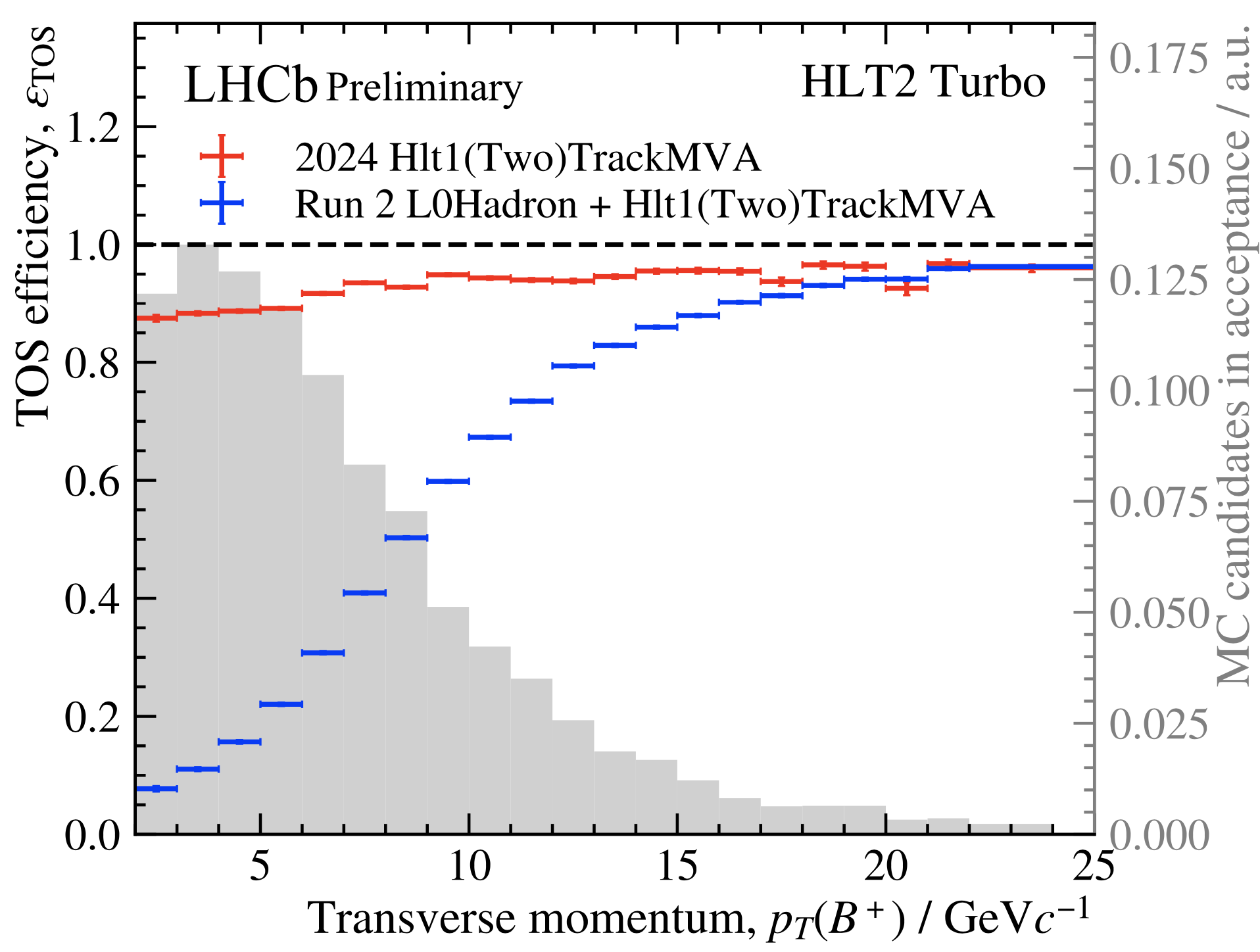
Figure 13: Comparison of trigger efficiencies for LHCb Run 2 and Run 3 taken from the LHCb public website: https://lbfence.cern.ch/alcm/public/figure/details/3837.

The trigger efficiencies for Run 3 are higher than those for Run 2, especially in the low $p_{T}$ region, as indicated in Fig. 13. The red points mark the efficiencies for Run 3 in 2024, and the blue points mark those for Run 2. The gray bars display the Monte-Carlo candidates in acceptance. The number of signal events can be deduced by convoluting the gray bars with the red or blue points. The signal events in Run 3 are then found to be roughly twice as many as those in Run 2. This figure depicts the trigger efficiencies for hadronic $B$ meson decays, which can be extrapolated to the case of hadronic $\Lambda_{b}$ baryon decays. According to the plan Chen:2021ftn, the LHCb will reach the integrated luminosity of 50 fb${}^{-1}$ at the end of Run 4. Since LHCb Run 3 is currently ongoing and its final integrated luminosity remains uncertain, we will estimate the signal events for the combined dataset of Run 3 and Run 4 by assuming that the conditions and performance of Run 4 are identical to those of Run 3. The ratio between the events from combined Run 3+4 and those from Run 2 is about $(50-9)$ fb${}^{-1}/6$ fb${}^{-1}\times 2\sim 14$, where the factor of 2 comes from the enhancement of trigger efficiencies for Run 3 TriggerEfficiency implied by Fig. 13. Taking into account the factor of 4 between the Run 2 and Run 1 data, the ratio of the events from Run 1+2+3+4 to those from Run 1 is nearly $1+4+4\times 14\sim 60$. That is, the total signal events of $\Lambda_{b}\to pa_{1}$ and $pK_{1}$ from the full Run 1+2+3+4 data can attain $800\times 60=48000$ and $1000\times 60=60000$, respectively.

Table 16: Predictions for $A_{UD}$ and $A_{UD}^{CP}$ in the $\Lambda_{b}\to pa_{1}$, $pK_{1}$ decays.

	$\Lambda_{b}\to pa_{1}$	$\Lambda_{b}\to pK_{1}(\theta_{K}=30^{\circ})$	$\Lambda_{b}\to pK_{1}(\theta_{K}=60^{\circ})$
$A_{UD}$	$(-9^{+2}_{-2})\%$	$(-19^{+4}_{-4})\%$	$(-24^{+6}_{-5})\%$
$A_{UD}^{CP}$	$(-24^{+8}_{-13})\%$	$(+26^{+4}_{-10})\%$	$(+40^{+4}_{-9})\%$

Both the $A_{UD}$ and $A_{UD}^{CP}$ values are essential for evaluating the experimental sensitivities, whose predictions are provided in Table 16. Recall the definition of $A_{UD}$,

$$\begin{split}A_{UD}=\frac{\Gamma(\cos\theta>0)-\Gamma(\cos\theta<0)}{\Gamma(\cos\theta>0)+\Gamma(\cos\theta<0)}=\frac{N_{>}-N_{<}}{N_{>}+N_{<}},\end{split}$$ (78)

where $N$ are the numbers of signal events with $N_{>}=N(\cos\theta>0)$ and $N_{<}=N(\cos\theta<0)$. The statistical error of $A_{UD}$ follows the error propagation formula

$$\sigma_{A_{UD}} =\sqrt{\left(\frac{\partial A_{UD}}{\partial N_{>}}\right)^{2}\sigma_{N_{>}}^{2}+\left(\frac{\partial A_{UD}}{\partial N_{<}}\right)^{2}\sigma_{N_{<}}^{2}}$$

$$=\sqrt{\left(\frac{2N_{<}}{(N_{>}+N_{<})^{2}}\right)^{2}\sigma_{N_{>}}^{2}+\left(\frac{-2N_{>}}{(N_{>}+N_{<})^{2}}\right)^{2}\sigma_{N_{<}}^{2}},$$ (79)

with $\sigma_{N_{>,<}}$ being the statistical errors of $N_{>,<}$. The neglect of background events for a naive analysis leads to the approximate uncertainties $\sigma_{N_{>}}\approx\sqrt{N_{>}}$ and $\sigma_{N_{<}}\approx\sqrt{N_{<}}$. As a simple estimate of the uncertainties and experimental sensitivities, we assume $N_{>}=N_{<}=\overline{N}_{>}=\overline{N}_{<}=N_{\rm tot}/4$, where $N_{\rm tot}=48000$ for $\Lambda_{b}\to pa_{1}$ and $N_{\rm tot}=60000$ for $\Lambda_{b}\to pK_{1}$. The statistical uncertainty of $A_{UD}$ is then $\sigma_{A_{UD}}\approx\sqrt{2/N_{\rm tot}}$, inferring the experimental uncertainties $\sigma_{A_{UD}}(\Lambda_{b}\to pa_{1})\approx 0.65\%$ and $\sigma_{A_{UD}}(\Lambda_{b}\to pK_{1})\approx 0.58\%$ from the full Run 1+2+3+4 data.

The background effects are expected to be less than $30\%$ on $\sigma_{A_{UD}}$, as reflected by the LHCb data; the signal yields of $\Lambda_{b}\to p\pi\pi\pi$ are $6646\pm 105$ corresponding to the integrated luminosity of 3 fb${}^{-1}$ in LHCb:2016yco, and $27600\pm 200$ for 6.6 fb${}^{-1}$ in LHCb:2019oke, where the errors include background contributions. The uncertainties of the pure signal events $\sqrt{6646}=81.5$ and $\sqrt{27600}=166.1$ are lifted by $29\%$ to 105 and by $20\%$ to 200, respectively. Hence, the uncertainties are found to be $\sigma_{A_{UD}}(\Lambda_{b}\to pa_{1})\approx 0.85\%$ and $\sigma_{A_{UD}}(\Lambda_{b}\to pK_{1})\approx 0.75\%$, amplified by a factor of 1.3.

We then proceed to the statistical uncertainty of $A_{UD}^{CP}=(A_{UD}+\overline{A}_{UD})/(A_{UD}-\overline{A}_{UD})$. Note that the quantity $\overline{A}_{UD}$ acquires an opposite sign relative to $A_{UD}$ under the parity transformation, because $A_{UD}$ is parity-odd. Analogous to Eq. (79), the uncertainty of $A_{UD}^{CP}$ is derived from

$$\sigma_{A_{UD}^{CP}}=\sqrt{\left(\frac{\partial A_{UD}^{CP}}{\partial A_{UD}}\right)^{2}\sigma_{A_{UD}}^{2}+\left(\frac{\partial A_{UD}^{CP}}{\partial\overline{A}_{UD}}\right)^{2}\sigma_{\overline{A}_{UD}}^{2}}\approx\frac{1}{\sqrt{2}|A_{UD}|}\sigma_{A_{UD}},$$ (80)

where the last expression is justified by the assumptions $\overline{A}_{UD}=-A_{UD}$ and $\sigma_{\overline{A}_{UD}}=\sigma_{A_{UD}}$. The magnitude of $A_{UD}$ is crucial for obtaining the uncertainty of $A_{UD}^{CP}$. The insertion of the central values of $A_{UD}$ in Table 16 yields the statistical uncertainties of $A_{UD}^{CP}$, $\sigma_{A_{UD}^{CP}}(\Lambda_{b}\to pa_{1})\approx\frac{0.85\%}{\sqrt{2}\times 9\%}=6.7\%$, $\sigma_{A_{UD}^{CP}}(\Lambda_{b}\to pK_{1}(\theta_{K}=30^{\circ}))\approx\frac{0.75\%}{\sqrt{2}\times 19\%}=2.8\%$ and $\sigma_{A_{UD}^{CP}}(\Lambda_{b}\to pK_{1}(\theta_{K}=60^{\circ}))\approx\frac{0.75\%}{\sqrt{2}\times 24\%}=2.2\%$.

Considering the differences of event numbers between particles and antiparticles caused by direct CPVs, between $N_{>}$ and $N_{<}$ caused by $A_{UD}$, and between $A_{UD}$ and $\overline{A}_{UD}$ arising from $A_{UD}^{CP}$, we refine the above crude estimates, arriving at the uncertainties $\sigma_{A_{UD}^{CP}}(\Lambda_{b}\to pa_{1})=5.2\%$, $\sigma_{A_{UD}^{CP}}(\Lambda_{b}\to pK_{1}(\theta_{K}=30^{\circ}))=3.8\%$ and $\sigma_{A_{UD}^{CP}}(\Lambda_{b}\to pK_{1}(\theta_{K}=60^{\circ}))=3.5\%$. The decrease of $\sigma_{A_{UD}^{CP}}(\Lambda_{b}\to pa_{1})$ and the increase of $\sigma_{A_{UD}^{CP}}(\Lambda_{b}\to pK_{1})$ stem from the negativity of ${A_{UD}^{CP}}(\Lambda_{b}\to pa_{1})$ and the positivity of ${A_{UD}^{CP}}(\Lambda_{b}\to pK_{1})$, respectively. Referring to the predicted $A_{UD}^{CP}$ in Table 16, we conclude that the CPV induced by the up-down asymmetry in $\Lambda_{b}\to pK_{1}$ could attain a statistic significance greater than $5\sigma$, while the CPV in $\Lambda_{b}\to pa_{1}$ is at the edge of $5\sigma$.

At last, we come to the issue of systematic uncertainties. We can learn from the measurements of $\hat{T}$-odd triple-product-asymmetry CPVs of $\Lambda_{b}\to p\pi^{-}\pi^{+}\pi^{-}$ in LHCb:2016yco and  LHCb:2019oke, which are defined as $C_{\hat{T}}=\vec{p}_{p}\cdot(\vec{p}_{\pi_{\rm fast}^{-}}\times\vec{p}_{\pi^{+}})$ for the $\hat{T}$-odd triple product of final-state particle momenta in the $\Lambda_{b}$ rest frame. Note that the quasi-time reversal transformation $\hat{T}$ reverses particle spins and momenta, while maintaining the initial and final states. The definitions of the triple product asymmetries (TPAs)

$$A_{\hat{T}}=\frac{N(C_{\hat{T}}>0)-N(C_{\hat{T}}<0)}{N(C_{\hat{T}}>0)+N(C_{\hat{T}}<0)},~~~~\bar{A}_{\hat{T}}=\frac{\bar{N}(-\bar{C}_{\hat{T}}>0)-\bar{N}(-\bar{C}_{\hat{T}}<0)}{\bar{N}(-\bar{C}_{\hat{T}}>0)+\bar{N}(-\bar{C}_{\hat{T}}<0)},$$ (81)

are similar to that for the up-down asymmetries in Eq. (76). The $\hat{T}$-odd $CP$- and $P$-violating asymmetries,

$$a_{CP}^{\hat{T}\text{-odd}}=\frac{1}{2}(A_{\hat{T}}-\bar{A}_{\hat{T}}),~~~~a_{P}^{\hat{T}\text{-odd}}=\frac{1}{2}(A_{\hat{T}}+\bar{A}_{\hat{T}}),$$ (82)

correspond to the numerator and the denominator, respectively, of the definition for $A_{CP}^{UD}$ in Eq. (77).

It has been known that the main sources of systematic uncertainties in the TPA analysis include selection criteria, reconstruction and detector acceptance based on the control sample of $\Lambda_{b}^{0}\to\Lambda_{c}^{+}(\to pK^{-}\pi^{+})\pi^{-}$. The systematic uncertainties are evaluated as $0.32\%$ for both $a_{CP}^{\hat{T}\text{-odd}}$ and $a_{P}^{\hat{T}\text{-odd}}$ with the Run 1 data in LHCb:2016yco, and $0.2\%$ with more data in LHCb:2019oke. The systematic uncertainties of both $A_{UD}+\bar{A}_{UD}$ and $A_{UD}-\bar{A}_{UD}$ can thus be taken as $0.2\%$ under the assumption that it is unchanged with more data samples. Using the error propagation formula with the fully positive correlation between $A_{UD}+\bar{A}_{UD}$ and $A_{UD}-\bar{A}_{UD}$, we obtain the systematic uncertainty of $A_{CP}^{UD}$ as about $0.2\%/(2|A_{UD}|)$. Namely, the systematic uncertainties of $A_{CP}^{UD}$ are $1.1\%$ for $\Lambda_{b}\to pa_{1}$, $0.5\%$ for $\Lambda_{b}\to pK_{1}(\theta_{K}=30^{\circ})$ and $0.4\%$ for $\Lambda_{b}\to pK_{1}(\theta_{K}=60^{\circ})$, which are less than the statistic uncertainties. Therefore, there is a great chance to identify the order-of-$20\%\sim 40\%$ up-down asymmetric CPVs in $\Lambda_{b}\to pa_{1}$ and $pK_{1}$ in the near future, and to establish CPVs in baryon decays.

IV Summary

We have performed the first full QCD analysis on two-body hadronic $\Lambda_{b}\to ph$ decays in the PQCD approach. We calculated the various topological amplitudes, including their strong phases, by incorporating the higher-twist hadron DAs. It is found that the subleading power corrections are in fact sizable in heavy baryon decays.

Our predictions for the total and partial-wave CPVs of the considered modes are summarized and compared with the available data for bottom hadron decays in Fig. 14 Han:2024kgz. We elucidated the mechanism responsible for the measured small CPVs in $\Lambda_{b}\to p\pi^{-},pK^{-}$, in contrast to the sizable CPVs in the similar $B$ meson decays. The partial-wave CPVs in $\Lambda_{b}\to p\pi^{-}$ attains $10\%$ potentially, but the destruction between them leads to the tiny CPV. The direct CPV of $\Lambda_{b}\to pK^{-}$ is primarily attributed to the modest $S$-wave CPV.

We have extended our investigation to the CPVs in the modes with vector and axial-vector final states. The partial-wave CPVs of the $\Lambda_{b}\to pV$, $pA$ decays also exceed $10\%$; for examples, the $P_{2}\text{-wave}$ CPVs of $\Lambda_{b}\to p\rho^{-}$ and $pa_{1}^{-}(1260)$ are $17\%$ and $-24\%$, respectively; the $(D+S^{L})\text{-wave}$ CPV of $\Lambda_{b}\to pK^{*-}$ is $27\%$; the partial-wave CPVs of $\Lambda_{b}\to pK^{-}_{1}(1270)$ even amount to the order of $30\%$. Nevertheless, the direct CPVs of the $\Lambda_{b}\to pK^{*-}$, $pa_{1}^{-}(1260)$ and $pK_{1}(1270)$ decays diminish as well, which trace back to the strong cancellation of the major $(D+S^{L})$- and $P_{1}\text{-wave}$ CPVs, like the $\Lambda_{b}\to p\pi^{-}$ case.

Our work suggests that certain partial-wave CPVs in bottom baryon decays, especially those related to angular distributions, can be sufficiently significant and probed to establish baryon CPVs. The decay asymmetry parameters of two-body $\Lambda_{b}$ modes are also predicted for future experimental confrontations. It opens avenues for deeply understanding the dynamics in heavy baryon decays and their CPVs. The rich data samples and complicated dynamics in multi-body bottom baryon decays offer remarkable prospects for exploring baryon CPVs.

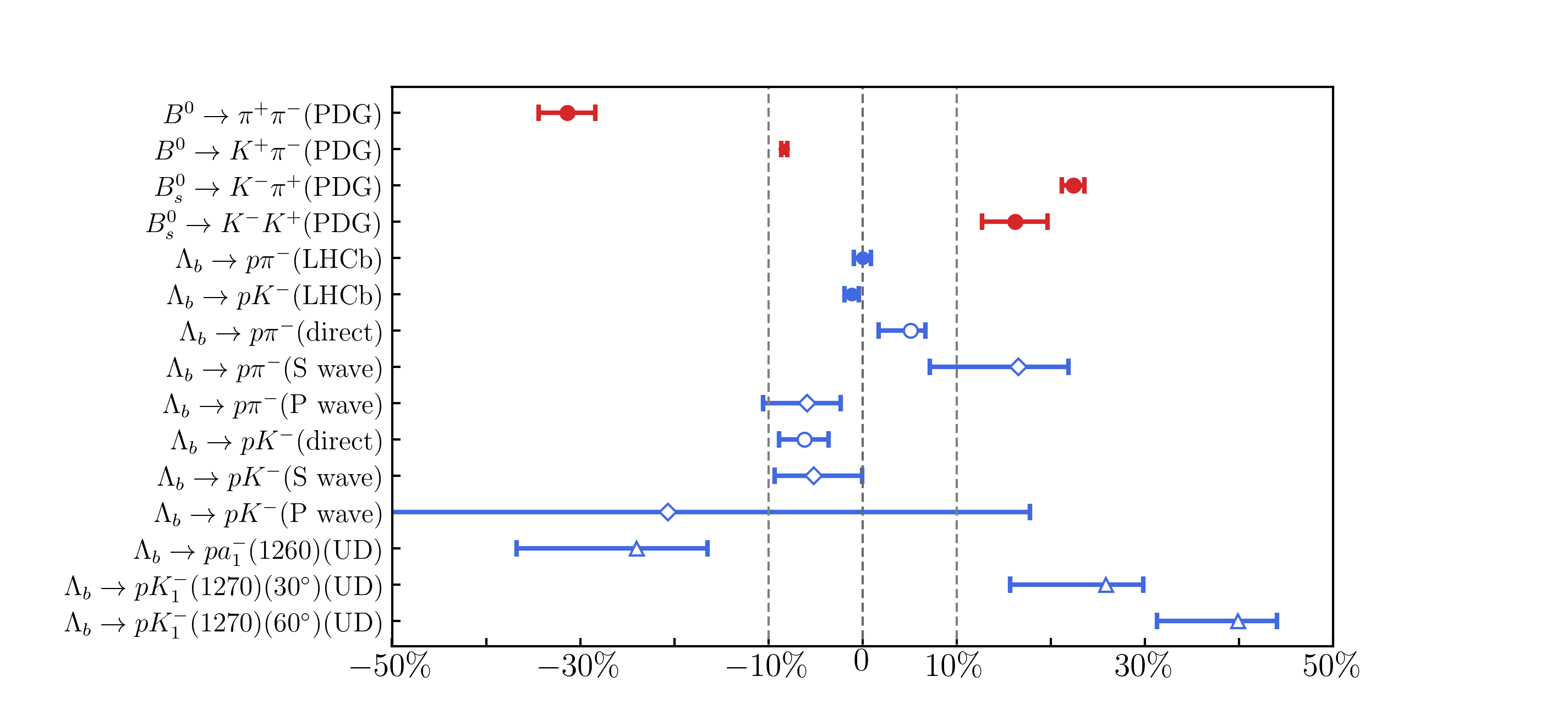
Figure 14: CPVs measured in $B$ meson and $\Lambda_{b}\to p\pi^{-},pK^{-}$ decays, and our predictions.

Appendix A Auxiliary functions

The auxiliary functions $F_{1,2,3,4}$ as the results of the Fourier transformation of the hard decay kernels from the $k_{T}$ space to the $b$ space are collected below:

$$\begin{split}&F_{1}(A,b)=\int d^{2}k_{T}\frac{e^{i\textbf{k}_{T}\cdot\textbf{b}}}{k^{2}+A}=2\pi\left\{K_{0}(\sqrt{Ab^{2}})\Theta(A)+\frac{i\pi}{2}H_{0}^{(1)}(\sqrt{-Ab^{2}})\Theta(-A)\right\},\end{split}$$ (83)

$$\begin{split}F_{2}(A,B,b)&=\int d^{2}k_{T}\frac{e^{i\textbf{k}_{T}\cdot\textbf{b}}}{(k^{2}+A)(k^{2}+B)}\\ &=\int_{0}^{1}dz\frac{\pi b}{\sqrt{|Z_{1}|}}\left\{K_{1}(\sqrt{Z_{1}b^{2}})\Theta(Z_{1})-\frac{i\pi}{2}H_{1}^{(1)}(\sqrt{-Z_{1}b^{2}})\Theta(-Z_{1})\right\},\end{split}$$ (84)

$$\begin{split}&F_{3}(A,B,C,b_{1},b_{2})=\int d^{2}k_{1T}\int d^{2}k_{2T}\frac{e^{i(\textbf{k}_{1T}\cdot\textbf{b}_{1}+\textbf{k}_{2T}\cdot\textbf{b}_{2})}}{(k_{1}^{2}+A)(k_{2}^{2}+B)((k_{1}+k_{2})^{2}+C)}\\ &=\int_{0}^{1}\frac{dz_{1}dz_{2}}{z_{1}(1-z_{1})}\frac{\pi^{2}\sqrt{X_{2}}}{\sqrt{|Z_{2}|}}\left\{K_{1}(\sqrt{X_{2}Z_{2}})\Theta(Z_{2})-\frac{i\pi}{2}H_{1}^{(1)}(\sqrt{-X_{2}Z_{2}})\Theta(-Z_{2})\right\},\end{split}$$ (85)

$$\begin{split}&F_{4}(A,B,C,D,b_{1},b_{2},b_{3})=\int d^{2}k_{1T}\int d^{2}k_{2T}\int d^{2}k_{3T}\frac{e^{i(\textbf{k}_{1T}\cdot\textbf{b}_{1}+\textbf{k}_{2T}\cdot\textbf{b}_{2}+\textbf{k}_{3T}\cdot\textbf{b}_{3})}}{(k_{1}^{2}+A)(k_{2}^{2}+B)(k_{3}^{2}+C)((k_{1}+k_{2}+k_{3})^{2}+D)}\\ &=\int_{0}^{1}\frac{dz_{1}dz_{2}dz_{3}}{z_{1}z_{2}(1-z_{1})(1-z_{2})}\frac{\pi^{3}\sqrt{X_{3}}}{\sqrt{|Z_{3}|}}\left\{K_{1}(\sqrt{X_{3}Z_{3}})\Theta(Z_{3})-\frac{i\pi}{2}H_{1}^{(1)}(\sqrt{-X_{3}Z_{3}})\Theta(-Z_{3})\right\}.\end{split}$$ (86)

In the above expressions $H_{v}^{(1)}(z)$ is the Hankel function of the first kind,

$$H_{v}^{(1)}(z)=J_{v}(z)+iY_{v}(z),$$ (87)

where $J_{v}(z)$ ($Y_{v}(z)$) is the Bessel function of the first (second) kind, and $K_{v}(z)$ is the modified Bessel function of second kind. The variables $Z_{1}$, $Z_{2}$, $Z_{3}$ and $X_{2}$, $X_{3}$ read

$$\begin{split}Z_{1}=&Az+B(1-z),\\ Z_{2}=&A(1-z_{2})+\frac{z_{2}}{z_{1}(1-z_{1})}\left[B(1-z_{1})+Cz_{1}\right],\\ Z_{3}=&A(1-z_{3})+\frac{z_{3}}{z_{2}(1-z_{2})}\left\{B(1-z_{2})+\frac{z_{2}}{z_{1}(1-z_{1})}\left[C(1-z_{1})+Dz_{1}\right]\right\},\\ X_{2}=&(b_{1}-z_{1}b_{2})^{2}+\frac{z_{1}(1-z_{1})}{z_{2}}b_{2}^{2},\\ X_{3}=&\left[b_{1}-b_{2}z_{2}-b_{3}z_{1}(1-z_{2})\right]^{2}+\frac{z_{2}(1-z_{2})}{z_{3}}(b_{2}-b_{3}z_{1})^{2}+\frac{z_{1}(1-z_{1})z_{2}(1-z_{2})}{z_{2}z_{3}}b_{3}^{2},\end{split}$$ (88)

with the Feynman parameters $z$’s. The above auxiliary functions appear in the PQCD factorization formulas for two-body hadronic $\Lambda_{b}$ baryon decays.

Appendix B Decay amplitudes

We present the PQCD factorization formula for each topological diagram, whose hard kernel involves two virtual gluons at the lowest order of the strong coupling $\alpha_{s}$. The Feynman diagrams to be evaluated are shown in Figs. 15, 17, 16, LABEL:fig:feynmanB and LABEL:fig:feynmanPd, where the gluon in black stays fixed, while the gluon in red has one fixed end with another attaching to a cross at various locations. A Feynman diagram is labeled by the crossed vertex. For instance, the upper-left diagram in Fig. 15 is labeled as $a3$. We provide the formula for one typical diagram in each topology involved in the $\Lambda_{b}\to p\pi^{-},pK^{-}$ decay. The amplitudes for the other modes $\Lambda_{b}\to p\rho^{-},pK^{\ast-},pa_{1}^{-},pK_{1}^{-}$ from the same topology are similar, but with different meson DAs.

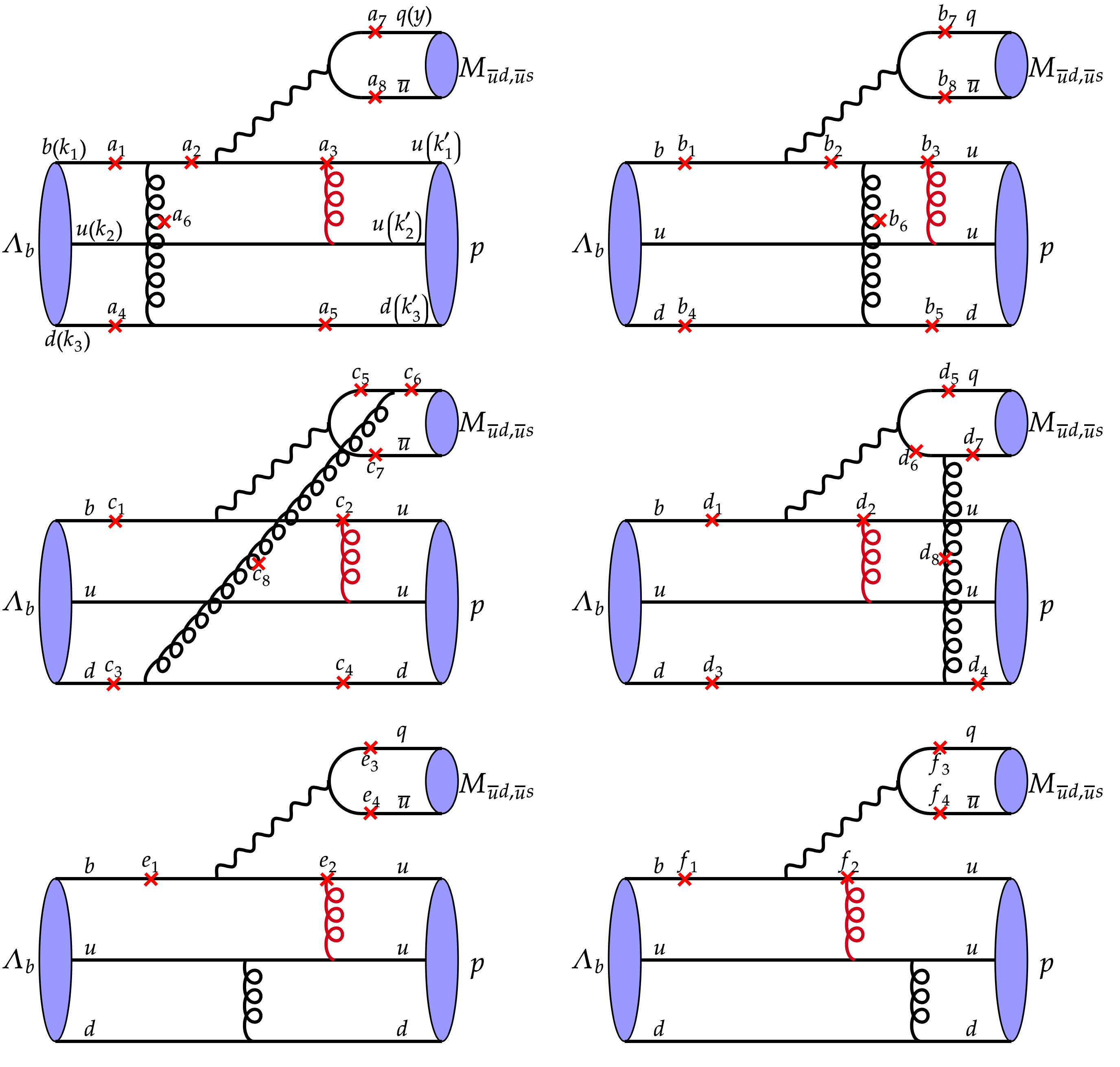
Figure 15: Feynman diagrams contributing to the external-$W$ emission topology $T$.

There are $40$ Feynman diagrams from the $T$ topology in Fig. 15, among which $16$ are factorizable without hard gluons attaching to the emitted meson, and $24$ are nonfactorizable. Applying the Feriz transformation to Fig. 15 and replacing the tree operators by the penguin ones, we acquire the diagrams for the $PC_{1}$ topology. The formula for the sum of the factorizable $T(b2)$ diagram and the corresponding $PC_{1}$ diagram is written as

$$\begin{split}&\mathcal{A}_{T(b2)+PC_{1}(b2)}=\frac{8}{3}\frac{-i}{128N_{c}^{2}}\int[dx]\int[dx^{\prime}]\frac{1}{(2\pi)^{5}}\int b_{1}db_{1}\int b_{2}^{\prime}db_{2}^{\prime}\int b_{3}^{\prime}db_{3}^{\prime}(4\pi\alpha_{s}(t^{T(b2)}))^{2}\\ &(M_{T(b2)}+M_{PC_{1}(b2)})F_{1}(C,b_{3}^{\prime})F_{3}(A,B,D,b_{1},b_{2}^{\prime})\text{exp}[-S^{T(b2)}([x],[x^{\prime}],y,[b],[b^{\prime}],b_{q})].\end{split}$$ (89)

The auxiliary functions $F_{i}$, with arguments

$$A=m_{\Lambda_{b}}^{2}(x_{2}+x_{3}),\quad B=m_{\Lambda_{b}}^{2}x_{3}(x_{1}^{\prime}+x_{3}^{\prime}),\quad C=m_{\Lambda_{b}}^{2}x_{3}x_{3}^{\prime},\quad D=m_{\Lambda_{b}}^{2}x_{2}x_{2}^{\prime},$$ (90)

from the internal particle propagators, have been given in Appendix. A. The functions

$$\begin{split}M_{T(b2)}=&\frac{G_{F}}{\sqrt{2}}\left\{V_{ub}V_{uq}^{\ast}\left[\frac{1}{3}C_{1}+C_{2}\right]\right\}M_{T(b2)}^{LL},\\ M_{PC_{1}(b2)}=&-\frac{G_{F}}{\sqrt{2}}\left\{V_{tb}V_{tq}^{\ast}\left[\frac{1}{3}C_{3}+C_{4}+\frac{1}{3}C_{9}+C_{10}\right]\right\}M_{T(b2)}^{LL}\\ &-\frac{G_{F}}{\sqrt{2}}\left\{V_{tb}V_{tq}^{\ast}\left[-\frac{2}{3}C_{5}-2C_{6}-\frac{2}{3}C_{7}-C_{8}\right]\right\}M_{T(b2)}^{SP}.\end{split}$$ (91)

are associated with the tree and penguin contributions, respectively, where the matrix element $M_{T(b2)}^{LL}$($M_{T(b2)}^{SP}$) corresponds to the insertion of the $(V-A)\otimes(V-A)$($(S-P)\otimes(S+P)$) operator. We display their explicit expressions as follows,

$$M_{T(b2)}^{LL}\equiv\langle h|(\bar{q}u)_{V-A}|0\rangle\langle p|(\bar{u}b)_{V-A}|\Lambda_{b}\rangle_{T(b2)}$$

$$= \Big{\{}8if_{P}m_{\Lambda_{b}}^{4}\psi_{4}T_{1}x_{3}+m_{p}m_{\Lambda_{b}}^{3}(-2if_{P}\psi_{3}^{-+}x_{3}(P_{1}+S_{1}+2T_{2}+T_{3}-T_{7})-2if_{P}\psi_{3}^{+-}x_{3}(-A_{3}+V_{3}))$$

$$+2if_{P}m_{p}^{3}m_{\Lambda_{b}}\psi_{3}^{-+}(x_{1}^{\prime}+x_{3}^{\prime})(A_{6}+V_{6})+m_{p}^{2}m_{\Lambda_{b}}^{2}(-4if_{P}\psi_{2}x_{3}(-A_{4}-A_{5}-V_{4}+V_{5})$$

$$+4if_{P}\psi_{4}(x_{1}^{\prime}+x_{3}^{\prime})(-A_{4}-A_{5}+P_{2}-S_{2}-T_{4}-T_{8}-V_{4}+V_{5}))\Big{\}}$$

$$+\Big{\{}8if_{P}m_{\Lambda_{b}}^{4}\psi_{4}T_{1}x_{3}+m_{p}m_{\Lambda_{b}}^{3}(2if_{P}\psi_{3}^{-+}x_{3}(-P_{1}-S_{1}-2T_{2}-T_{3}+T_{7})+2if_{P}\psi_{3}^{+-}x_{3}(A_{3}-V_{3}))$$

$$+2if_{P}m_{p}^{3}m_{\Lambda_{b}}\psi_{3}^{-+}(x_{1}^{\prime}+x_{3}^{\prime})(A_{6}+V_{6})+m_{p}^{2}m_{\Lambda_{b}}^{2}(4if_{P}\psi_{2}x_{3}(A_{4}+A_{5}+V_{4}-V_{5})$$

$$-4if_{P}\psi_{4}(x_{1}^{\prime}+x_{3}^{\prime})(A_{4}+A_{5}-P_{2}+S_{2}+T_{4}+T_{8}+V_{4}-V_{5}))\Big{\}}\gamma_{5},$$ (92)

$$M_{T(b2)}^{SP}\equiv\langle h|(\bar{q}u)_{S+P}|0\rangle\langle p|(\bar{u}b)_{S-P}|\Lambda_{b}\rangle_{T(b2)}$$

$$=\Big{\{}-2if_{P}m_{0}^{P}(m_{\Lambda_{b}}^{3}x_{3}(4\psi_{4}T_{1}+\psi_{3}^{+-}(A_{1}+V_{1})(x_{2}+x_{3}))+m_{p}^{3}(A_{6}\psi_{3}^{-+}+\psi_{3}^{-+}V_{6}+4\psi_{2}T_{6}(x_{2}+x_{3}))$$

$$(x_{1}^{\prime}+x_{3}^{\prime})-m_{p}m_{\Lambda_{b}}^{2}(\psi_{3}^{-+}(P_{1}+S_{1}+2T_{2}+T_{3}-T_{7})x_{3}+\psi_{3}^{+-}(-A_{3}+V_{3})x_{3}+2\psi_{2}(A_{2}+A_{3}$$

$$-P_{1}+S_{1}+T_{3}+T_{7}-V_{2}+V_{3})x_{3}(x_{2}+x_{3})-2\psi_{4}(A_{2}+A_{3}-V_{2}+V_{3})(x_{2}+x_{3})(x_{1}^{\prime}+x_{3}^{\prime}))$$

$$+m_{p}^{2}m_{\Lambda_{b}}(2\psi_{2}(A_{4}+A_{5}+V_{4}-V_{5})x_{3}-2\psi_{4}(A_{4}+A_{5}-P_{2}+S_{2}+T_{4}+T_{8}+V_{4}-V_{5})(x_{1}^{\prime}+x_{3}^{\prime})$$

$$-\psi_{3}^{+-}(P_{2}+S_{2}+T_{4}+2T_{5}-T_{8})(x_{2}+x_{3})(x_{1}^{\prime}+x_{3}^{\prime})+\psi_{3}^{-+}(A_{4}-V_{4})(x_{2}+x_{3})(x_{1}^{\prime}+x_{3}^{\prime})))\Big{\}}$$

$$+\Big{\{}2if_{P}m_{0}^{P}(m_{\Lambda_{b}}^{3}(4\psi_{4}T_{1}x_{3}-\psi_{3}^{+-}(A_{1}+V_{1})x_{3}(x_{2}+x_{3}))+m_{p}^{3}(A_{6}\psi_{3}^{-+}+\psi_{3}^{-+}V_{6}-4\psi_{2}T_{6}(x_{2}+x_{3}))$$

$$(x_{1}^{\prime}+x_{3}^{\prime})-m_{p}m_{\Lambda_{b}}^{2}(\psi_{3}^{-+}(P_{1}+S_{1}+2T_{2}+T_{3}-T_{7})x_{3}+\psi_{3}^{+-}(-A_{3}+V_{3})x_{3}-2\psi_{2}(A_{2}+A_{3}$$

$$-P_{1}+S_{1}+T_{3}+T_{7}-V_{2}+V_{3})x_{3}(x_{2}+x_{3})+2\psi_{4}(A_{2}+A_{3}-V_{2}+V_{3})(x_{2}+x_{3})(x_{1}^{\prime}+x_{3}^{\prime}))$$

$$+m_{p}^{2}m_{\Lambda_{b}}(2\psi_{2}(A_{4}+A_{5}+V_{4}-V_{5})x_{3}-2\psi_{4}(A_{4}+A_{5}-P_{2}+S_{2}+T_{4}+T_{8}+V_{4}-V_{5})(x_{1}^{\prime}+x_{3}^{\prime})$$

$$+\psi_{3}^{+-}(P_{2}+S_{2}+T_{4}+2T_{5}-T_{8})(x_{2}+x_{3})(x_{1}^{\prime}+x_{3}^{\prime})-\psi_{3}^{-+}(A_{4}-V_{4})(x_{2}+x_{3})(x_{1}^{\prime}+x_{3}^{\prime})))\Big{\}}\gamma_{5}.$$ (93)

The non-factorizable $T(c7)$ diagram yields

$$\begin{split}\mathcal{A}_{T(c7)}=&\frac{-1}{128N_{c}^{2}}\frac{1}{\sqrt{2N_{c}}}\int[dx]\int[dx^{\prime}]\int dy\frac{1}{(2\pi)^{5}}\int b_{2}db_{2}\int b_{3}db_{3}\int b_{q}db_{q}(4\pi\alpha_{s}(t^{T(c7)}))^{2}\\ &(M_{T(c7)}+M_{PC_{1}(c7)})F_{4}(D,C,B,A,b_{2},b_{3},b_{q})\text{exp}[-S^{T(c7)}([x],[x^{\prime}],y,[b],[b^{\prime}],b_{q})],\end{split}$$ (94)

with the arguments,

$$A=m_{\Lambda_{b}}^{2}x_{3}^{\prime}(x_{3}-y),\quad B=m_{\Lambda_{b}}^{2}x_{2}^{\prime}(-1+x_{2}+y),\quad C=m_{\Lambda_{b}}^{2}x_{3}x_{3}^{\prime},\quad D=m_{\Lambda_{b}}^{2}x_{2}x_{2}^{\prime}.$$ (95)

The functions

$$\begin{split}M_{T(c7)}=&\frac{G_{F}}{\sqrt{2}}\left\{V_{ub}V_{uq}^{\ast}\left[f_{1}C_{1}+f_{2}C_{2}\right]\right\}M_{T(c7)}^{LL},\\ M_{PC_{1}(c7)}=&-\frac{G_{F}}{\sqrt{2}}\left\{V_{tb}V_{tq}^{\ast}\left[f_{1}C_{3}+f_{2}C_{4}+f_{1}C_{9}+f_{2}C_{10}\right]\right\}M_{T(c7)}^{LL}\\ &-\frac{G_{F}}{\sqrt{2}}\left\{V_{tb}V_{tq}^{\ast}\left[f_{1}C_{5}+f_{2}C_{6}+f_{1}C_{7}+f_{2}C_{8}\right]\right\}M_{T(c7)}^{LR},\end{split}$$ (96)

where $f_{1}=8/3$ and $f_{2}=-2$ are the color factors, and the superscript $LR$ refers to the contribution from the $(V-A)\otimes(V+A)$ operator, contain the matrix elements

$$M_{T(c7)}^{LL}\equiv\langle ph|(\bar{q}b)_{V-A}(\bar{u}u)_{V-A}|\Lambda_{b}\rangle_{T(c7)}$$

$$= \Big{\{}8m_{\Lambda_{b}}(4m_{p}^{3}\psi_{2}T_{6}x_{2}^{\prime}x_{3}^{\prime}+m_{p}^{2}m_{\Lambda_{b}}x_{3}^{\prime}((A_{4}\psi_{3}^{-+}-2\psi_{3}^{+-}T_{5}-\psi_{3}^{-+}V_{4})x_{2}^{\prime}-2\psi_{2}(P_{2}-S_{2}+T_{4}+T_{8})$$

$$(-1+x_{2}+y))+m_{\Lambda_{b}}^{3}(x_{3}-y)(A_{1}\psi_{3}^{-+}x_{2}^{\prime}+\psi_{3}^{-+}V_{1}x_{2}^{\prime}-2A_{1}\psi_{2}(-1+x_{2}+y)+2\psi_{2}(2T_{1}+V_{1})$$

$$(-1+x_{2}+y))+m_{p}m_{\Lambda_{b}}^{2}(2\psi_{4}(A_{3}+V_{3})x_{2}^{\prime}x_{3}^{\prime}-2\psi_{2}(P_{1}-S_{1}+T_{3}+T_{7})x_{2}^{\prime}(x_{3}-y)$$

$$+\psi_{3}^{+-}(P_{1}+S_{1}+T_{3}-T_{7})x_{3}^{\prime}(-1+x_{2}+y)))\phi_{m}^{A}\Big{\}}$$

$$+\Big{\{}8m_{\Lambda_{b}}(-4m_{p}^{3}\psi_{2}T_{6}x_{2}^{\prime}x_{3}^{\prime}+m_{p}^{2}m_{\Lambda_{b}}x_{3}^{\prime}((-A_{4}\psi_{3}^{-+}+2\psi_{3}^{+-}T_{5}+\psi_{3}^{-+}V_{4})x_{2}^{\prime}+2\psi_{2}(-P_{2}+S_{2}-T_{4}-T_{8})$$

$$(-1+x_{2}+y))-m_{\Lambda_{b}}^{3}(x_{3}-y)(A_{1}\psi_{3}^{-+}x_{2}^{\prime}+\psi_{3}^{-+}V_{1}x_{2}^{\prime}+2A_{1}\psi_{2}(-1+x_{2}+y)-2\psi_{2}(2T_{1}+V_{1})$$

$$(-1+x_{2}+y))+m_{p}m_{\Lambda_{b}}^{2}(-2\psi_{4}(A_{3}+V_{3})x_{2}^{\prime}x_{3}^{\prime}+2\psi_{2}(P_{1}-S_{1}+T_{3}+T_{7})x_{2}^{\prime}(x_{3}-y)$$

$$+\psi_{3}^{+-}(P_{1}+S_{1}+T_{3}-T_{7})x_{3}^{\prime}(-1+x_{2}+y)))\phi_{m}^{A}\Big{\}}\gamma_{5},$$ (97)

$$M_{T(c7)}^{LR}\equiv\langle ph|(\bar{q}b)_{V-A}(\bar{u}u)_{V+A}|\Lambda_{b}\rangle_{T(c7)}$$

$$= \Big{\{}8m_{0}(2m_{p}^{3}\psi_{2}(-((A_{6}-V_{6})x_{3}^{\prime}(-1+x_{2}+y)(\phi_{m}^{P}-\phi_{m}^{T}))+2T_{6}x_{2}^{\prime}(x_{3}-y)(\phi_{m}^{P}+\phi_{m}^{T}))-2m_{\Lambda_{b}}^{3}\psi_{4}(-2T_{1}x_{3}^{\prime}$$

$$(-1+x_{2}+y)(\phi_{m}^{P}-\phi_{m}^{T})+A_{1}x_{2}^{\prime}(x_{3}-y)(\phi_{m}^{P}+\phi_{m}^{T})-V_{1}x_{2}^{\prime}(x_{3}-y)(\phi_{m}^{P}+\phi_{m}^{T}))+m_{p}^{2}m_{\Lambda_{b}}(-2\psi_{3}^{+-}T_{5}x_{2}^{\prime}$$

$$(x_{3}-y)(\phi_{m}^{P}+\phi_{m}^{T})+\psi_{3}^{+-}x_{3}^{\prime}(-1+x_{2}+y)((A_{4}+A_{5}+P_{2}+S_{2}-T_{4}+T_{8}-V_{4}+V_{5})\phi_{m}^{P}$$

$$+(A_{4}-A_{5}+P_{2}+S_{2}-T_{4}+T_{8}-V_{4}-V_{5})\phi_{m}^{T})+\psi_{3}^{-+}(((A_{5}-2T_{5}-V_{4}+V_{5})x_{2}^{\prime}x_{3}+(P_{2}+S_{2}-T_{4}+T_{8})$$

$$(-1+x_{2})x_{3}^{\prime}-(A_{5}-2T_{5}-V_{4}+V_{5})x_{2}^{\prime}y+(P_{2}+S_{2}-T_{4}+T_{8})x_{3}^{\prime}y)\phi_{m}^{P}-((A_{5}-2T_{5}+V_{4}+V_{5})x_{2}^{\prime}x_{3}$$

$$+(P_{2}+S_{2}-T_{4}+T_{8})(-1+x_{2})x_{3}^{\prime}-(A_{5}-2T_{5}+V_{4}+V_{5})x_{2}^{\prime}y+(P_{2}+S_{2}-T_{4}+T_{8})x_{3}^{\prime}y)\phi_{m}^{T}$$

$$+A_{4}x_{2}^{\prime}(x_{3}-y)(\phi_{m}^{P}+\phi_{m}^{T}))-2\psi_{2}(-(((S_{2}+T_{4}+T_{8})x_{2}^{\prime}x_{3}+(A_{4}+V_{4})(-1+x_{2})x_{3}^{\prime}-(S_{2}+T_{4}+T_{8})x_{2}^{\prime}y$$

$$+(A_{4}+V_{4})x_{3}^{\prime}y)\phi_{m}^{P})+(-((S_{2}+T_{4}+T_{8})x_{2}^{\prime}x_{3})+(A_{4}+V_{4})(-1+x_{2})x_{3}^{\prime}+(S_{2}+T_{4}+T_{8})x_{2}^{\prime}y$$

$$+(A_{4}+V_{4})x_{3}^{\prime}y)\phi_{m}^{T}+P_{2}x_{2}^{\prime}(x_{3}-y)(\phi_{m}^{P}+\phi_{m}^{T})))+m_{p}m_{\Lambda_{b}}^{2}(\psi_{3}^{-+}((A_{2}+A_{3}+P_{1}+S_{1}-T_{3}+T_{7}+V_{2}-V_{3})x_{2}^{\prime}x_{3}$$

$$-2T_{2}(-1+x_{2})x_{3}^{\prime}-((A_{2}+A_{3}+P_{1}+S_{1}-T_{3}+T_{7}+V_{2}-V_{3})x_{2}^{\prime}+2T_{2}x_{3}^{\prime})y)\phi_{m}^{P}+\psi_{3}^{-+}((A_{2}-A_{3}-P_{1}$$

$$-S_{1}+T_{3}-T_{7}+V_{2}+V_{3})x_{2}^{\prime}x_{3}+2T_{2}(-1+x_{2})x_{3}^{\prime}+(-A_{2}+A_{3}+P_{1}+S_{1}-T_{3}+T_{7}-V_{2}-V_{3})x_{2}^{\prime}y+2T_{2}x_{3}^{\prime}y)\phi_{m}^{T}$$

$$+\psi_{3}^{+-}(((S_{1}-T_{3}+T_{7})x_{2}^{\prime}x_{3}+(A_{2}+A_{3}-2T_{2}+V_{2}-V_{3})(-1+x_{2})x_{3}^{\prime}-(S_{1}-T_{3}+T_{7})x_{2}^{\prime}y+(A_{2}+A_{3}$$

$$-2T_{2}+V_{2}-V_{3})x_{3}^{\prime}y)\phi_{m}^{P}+((S_{1}-T_{3}+T_{7})x_{2}^{\prime}x_{3}+(A_{2}-A_{3}-2T_{2}+V_{2}+V_{3})(-1+x_{2})x_{3}^{\prime}-(S_{1}-T_{3}+T_{7})x_{2}^{\prime}y$$

$$+(A_{2}-A_{3}-2T_{2}+V_{2}+V_{3})x_{3}^{\prime}y)\phi_{m}^{T}+P_{1}x_{2}^{\prime}(x_{3}-y)(\phi_{m}^{P}+\phi_{m}^{T}))+2\psi_{4}(-((P_{1}-S_{1}-T_{3}-T_{7})x_{3}^{\prime}(-1+x_{2}+y)$$

$$(\phi_{m}^{P}-\phi_{m}^{T}))+A_{3}x_{2}^{\prime}(x_{3}-y)(\phi_{m}^{P}+\phi_{m}^{T})+V_{3}x_{2}^{\prime}(x_{3}-y)(\phi_{m}^{P}+\phi_{m}^{T}))))\Big{\}}$$

$$+\Big{\{}8m_{0}(2m_{p}^{3}\psi_{2}(-((A_{6}-V_{6})x_{3}^{\prime}(-1+x_{2}+y)(\phi_{m}^{P}-\phi_{m}^{T}))+2T_{6}x_{2}^{\prime}(x_{3}-y)(\phi_{m}^{P}+\phi_{m}^{T}))+2m_{\Lambda_{b}}^{3}\psi_{4}(-2T_{1}x_{3}^{\prime}$$

$$(-1+x_{2}+y)(\phi_{m}^{P}-\phi_{m}^{T})+A_{1}x_{2}^{\prime}(x_{3}-y)(\phi_{m}^{P}+\phi_{m}^{T})-V_{1}x_{2}^{\prime}(x_{3}-y)(\phi_{m}^{P}+\phi_{m}^{T}))+m_{p}^{2}m_{\Lambda_{b}}(-2\psi_{3}^{+-}T_{5}x_{2}^{\prime}$$

$$(x_{3}-y)(\phi_{m}^{P}+\phi_{m}^{T})+\psi_{3}^{+-}x_{3}^{\prime}(-1+x_{2}+y)((A_{4}+A_{5}+P_{2}+S_{2}-T_{4}+T_{8}-V_{4}+V_{5})\phi_{m}^{P}$$

$$+(A_{4}-A_{5}+P_{2}+S_{2}-T_{4}+T_{8}-V_{4}-V_{5})\phi_{m}^{T})+\psi_{3}^{-+}(((A_{5}-2T_{5}-V_{4}+V_{5})x_{2}^{\prime}x_{3}+(P_{2}+S_{2}-T_{4}+T_{8})$$

$$(-1+x_{2})x_{3}^{\prime}-(A_{5}-2T_{5}-V_{4}+V_{5})x_{2}^{\prime}y+(P_{2}+S_{2}-T_{4}+T_{8})x_{3}^{\prime}y)\phi_{m}^{P}-((A_{5}-2T_{5}+V_{4}+V_{5})x_{2}^{\prime}x_{3}$$

$$+(P_{2}+S_{2}-T_{4}+T_{8})(-1+x_{2})x_{3}^{\prime}-(A_{5}-2T_{5}+V_{4}+V_{5})x_{2}^{\prime}y+(P_{2}+S_{2}-T_{4}+T_{8})x_{3}^{\prime}y)\phi_{m}^{T}$$

$$+A_{4}x_{2}^{\prime}(x_{3}-y)(\phi_{m}^{P}+\phi_{m}^{T}))+2\psi_{2}(-(((S_{2}+T_{4}+T_{8})x_{2}^{\prime}x_{3}+(A_{4}+V_{4})(-1+x_{2})x_{3}^{\prime}-(S_{2}+T_{4}+T_{8})x_{2}^{\prime}y$$

$$+(A_{4}+V_{4})x_{3}^{\prime}y)\phi_{m}^{P})+(-((S_{2}+T_{4}+T_{8})x_{2}^{\prime}x_{3})+(A_{4}+V_{4})(-1+x_{2})x_{3}^{\prime}+(S_{2}+T_{4}+T_{8})x_{2}^{\prime}y$$

$$+(A_{4}+V_{4})x_{3}^{\prime}y)\phi_{m}^{T}+P_{2}x_{2}^{\prime}(x_{3}-y)(\phi_{m}^{P}+\phi_{m}^{T})))-m_{p}m_{\Lambda_{b}}^{2}(\psi_{3}^{-+}((A_{2}+A_{3}+P_{1}+S_{1}-T_{3}+T_{7}+V_{2}-V_{3})x_{2}^{\prime}x_{3}$$

$$-2T_{2}(-1+x_{2})x_{3}^{\prime}-((A_{2}+A_{3}+P_{1}+S_{1}-T_{3}+T_{7}+V_{2}-V_{3})x_{2}^{\prime}+2T_{2}x_{3}^{\prime})y)\phi_{m}^{P}+\psi_{3}^{-+}((A_{2}-A_{3}-P_{1}$$

$$-S_{1}+T_{3}-T_{7}+V_{2}+V_{3})x_{2}^{\prime}x_{3}+2T_{2}(-1+x_{2})x_{3}^{\prime}+(-A_{2}+A_{3}+P_{1}+S_{1}-T_{3}+T_{7}-V_{2}-V_{3})x_{2}^{\prime}y+2T_{2}x_{3}^{\prime}y)\phi_{m}^{T}$$

$$+\psi_{3}^{+-}(((S_{1}-T_{3}+T_{7})x_{2}^{\prime}x_{3}+(A_{2}+A_{3}-2T_{2}+V_{2}-V_{3})(-1+x_{2})x_{3}^{\prime}-(S_{1}-T_{3}+T_{7})x_{2}^{\prime}y+(A_{2}+A_{3}$$

$$-2T_{2}+V_{2}-V_{3})x_{3}^{\prime}y)\phi_{m}^{P}+((S_{1}-T_{3}+T_{7})x_{2}^{\prime}x_{3}+(A_{2}-A_{3}-2T_{2}+V_{2}+V_{3})(-1+x_{2})x_{3}^{\prime}-(S_{1}-T_{3}+T_{7})x_{2}^{\prime}y$$

$$+(A_{2}-A_{3}-2T_{2}+V_{2}+V_{3})x_{3}^{\prime}y)\phi_{m}^{T}+P_{1}x_{2}^{\prime}(x_{3}-y)(\phi_{m}^{P}+\phi_{m}^{T}))-2\psi_{4}(-((P_{1}-S_{1}-T_{3}-T_{7})x_{3}^{\prime}(-1+x_{2}+y)$$

$$(\phi_{m}^{P}-\phi_{m}^{T}))+A_{3}x_{2}^{\prime}(x_{3}-y)(\phi_{m}^{P}+\phi_{m}^{T})+V_{3}x_{2}^{\prime}(x_{3}-y)(\phi_{m}^{P}+\phi_{m}^{T}))))\Big{\}}\gamma_{5}.$$ (98)

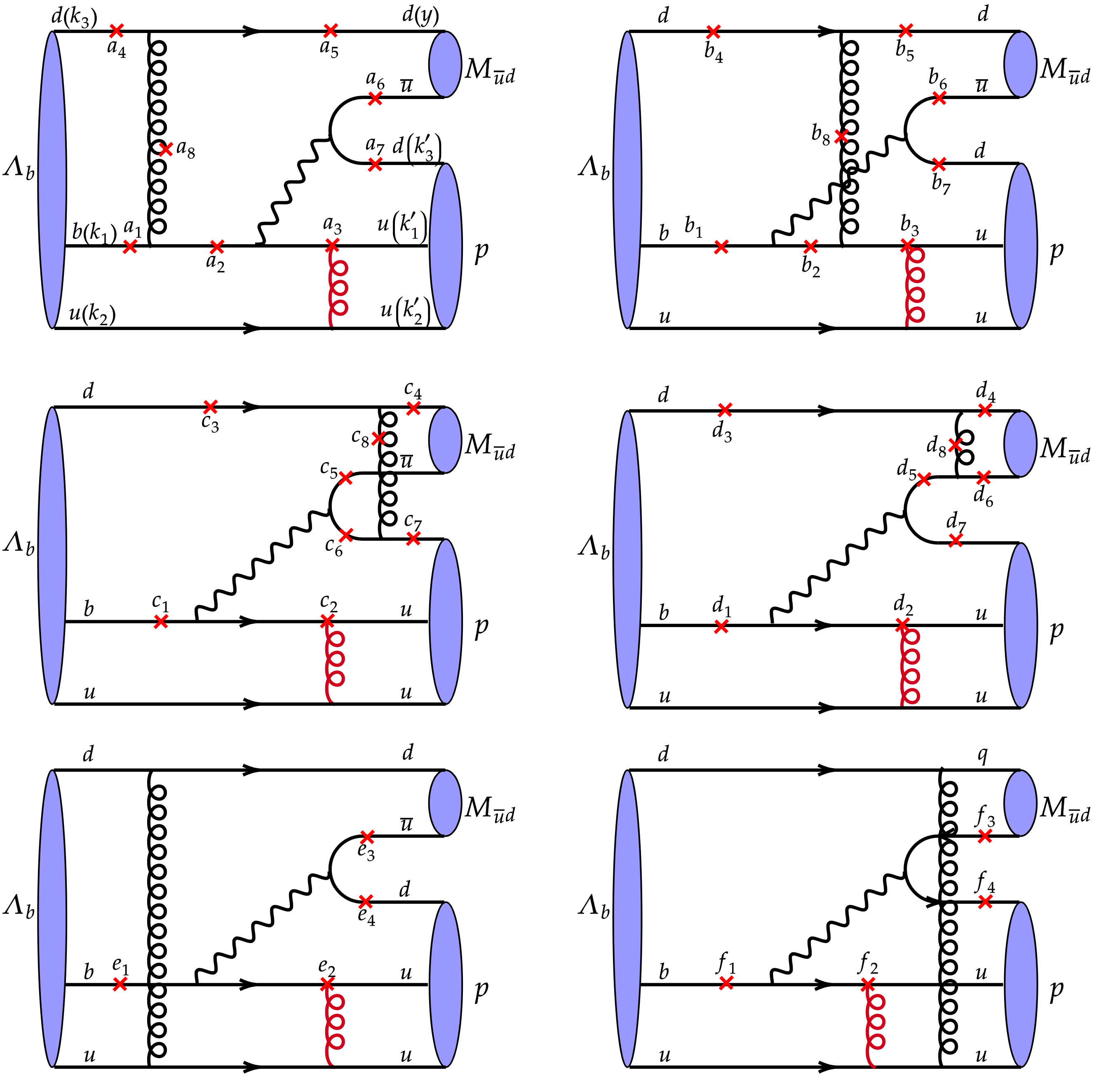
Figure 16: Feynman diagrams contributing to the $C_{2}$ topology.

For the $C_{2}(c7)$ diagram in Fig. 16, we have

$$\begin{split}\mathcal{A}_{C_{2}(c7)}=&\frac{-1}{128N_{c}^{2}}\frac{1}{\sqrt{2N_{c}}}\int[dx]\int[dx^{\prime}]\int dy\frac{1}{(2\pi)^{5}}\int b_{2}db_{2}\int b_{2}^{\prime}db_{2}^{\prime}\int b_{q}db_{q}(4\pi\alpha_{s}(t^{C_{2}(c7)}))^{2}\\ &(M_{C_{2}(c7)}+M_{PC_{2}(c7)})F_{1}(D,b_{2}^{\prime})F_{3}(A,C,B,b_{2},b_{2}^{\prime},b_{q})\text{exp}[-S^{C_{2}(c7)}([x],[x^{\prime}],y,[b],[b^{\prime}],b_{q})],\end{split}$$ (99)

with the arguments

$$A=m_{\Lambda_{b}}^{2}x_{2}(x_{2}^{\prime}+x_{2}^{\prime}),\quad B=m_{\Lambda_{b}}^{2}(x_{2}^{\prime}-x_{3}+x_{3}^{\prime})(x_{2}-y),\quad C=m_{\Lambda_{b}}^{2}x_{3}y,\quad D=m_{\Lambda_{b}}^{2}x_{2}x_{2}^{\prime}.$$ (100)

The functions

$$\begin{split}M_{C_{2}(c7)}=&\frac{G_{F}}{\sqrt{2}}\left\{V_{ub}V_{ud}^{\ast}\left[f_{1}C_{1}+f_{2}C_{2}\right]\right\}M_{C_{2}(c7)}^{LL},\\ M_{PC_{2}(c7)}=&-\frac{G_{F}}{\sqrt{2}}\left\{V_{tb}V_{td}^{\ast}\left[f_{1}C_{3}+f_{2}C_{4}+f_{1}C_{9}+f_{2}C_{10}\right]\right\}M_{C_{2}(c7)}^{LL}\\ &-\frac{G_{F}}{\sqrt{2}}\left\{V_{tb}V_{td}^{\ast}\left[-2f_{1}C_{5}-2f_{2}C_{6}-2f_{1}C_{7}-2f_{2}C_{8}\right]\right\}M_{C_{2}(c7)}^{SP},\end{split}$$ (101)

contain the color factors $f_{1}=-8/3$ and $f_{2}=-16/3$, and the matrix elements

$$M_{C_{2}(c7)}^{LL}\equiv\langle ph|(\bar{u}b)_{V-A}(\bar{d}u)_{V-A}|\Lambda_{b}\rangle_{C_{2}(c7)}$$

$$= \Big{\{}8m_{0}m_{p}^{3}\psi_{3}^{+-}(A_{6}-V_{6})(x_{2}^{\prime}+x_{3}^{\prime})(x_{2}^{\prime}-x_{3}+x_{3}^{\prime})(\phi_{m}^{P}-\phi_{m}^{T})+8m_{0}m_{\Lambda_{b}}^{3}\psi_{3}^{-+}(A_{1}-V_{1})x_{2}(x_{2}-y)$$

$$(\phi_{m}^{P}+\phi_{m}^{T})-8m_{p}m_{\Lambda_{b}}^{2}(m_{\Lambda_{b}}\psi_{3}^{-+}(P_{1}+S_{1}-2T_{2}-T_{3}+T_{7})(x_{2}^{\prime}+x_{3}^{\prime})(x_{2}-y)\phi_{m}^{A}-m_{0}\psi_{3}^{-+}(A_{3}+V_{3})x_{2}$$

$$(x_{2}^{\prime}-x_{3}+x_{3}^{\prime})(\phi_{m}^{P}-\phi_{m}^{T})+2m_{0}\psi_{2}(P_{1}+S_{1}-2T_{2}-T_{3}+T_{7})x_{2}(x_{2}-y)(\phi_{m}^{P}+\phi_{m}^{T})-2m_{0}\psi_{4}(P_{1}+S_{1}$$

$$-2T_{2}-T_{3}+T_{7})(x_{2}^{\prime}+x_{3}^{\prime})(x_{2}-y)(\phi_{m}^{P}+\phi_{m}^{T}))-8m_{p}^{2}m_{\Lambda_{b}}(-2\psi_{4}(x_{2}^{\prime}+x_{3}^{\prime})(x_{2}^{\prime}-x_{3}+x_{3}^{\prime})$$

$$(A_{5}m_{\Lambda_{b}}\phi_{m}^{A}-m_{\Lambda_{b}}V_{5}\phi_{m}^{A}-m_{0}(P_{2}+S_{2}-T_{4}-2T_{5}+T_{8})(\phi_{m}^{P}-\phi_{m}^{T}))+2\psi_{2}(A_{4}m_{\Lambda_{b}}(x_{2}^{\prime}+x_{3}^{\prime})(x_{2}-y)\phi_{m}^{A}$$

$$+m_{\Lambda_{b}}V_{4}(x_{2}^{\prime}+x_{3}^{\prime})(x_{2}-y)\phi_{m}^{A}-m_{0}(P_{2}+S_{2}-T_{4}-2T_{5}+T_{8})x_{2}(x_{2}^{\prime}-x_{3}+x_{3}^{\prime})(\phi_{m}^{P}-\phi_{m}^{T}))$$

$$-m_{0}\psi_{3}^{+-}(A_{4}+V_{4})(x_{2}^{\prime}+x_{3}^{\prime})(x_{2}-y)(\phi_{m}^{P}+\phi_{m}^{T}))\Big{\}}$$

$$+\Big{\{}-8m_{0}m_{p}^{3}\psi_{3}^{+-}(A_{6}-V_{6})(x_{2}^{\prime}+x_{3}^{\prime})(x_{2}^{\prime}-x_{3}+x_{3}^{\prime})(\phi_{m}^{P}-\phi_{m}^{T})+8m_{0}m_{\Lambda_{b}}^{3}\psi_{3}^{-+}(A_{1}-V_{1})x_{2}(x_{2}-y)$$

$$(\phi_{m}^{P}+\phi_{m}^{T})-8m_{p}m_{\Lambda_{b}}^{2}(m_{\Lambda_{b}}\psi_{3}^{-+}(P_{1}+S_{1}-2T_{2}-T_{3}+T_{7})(x_{2}^{\prime}+x_{3}^{\prime})(x_{2}-y)\phi_{m}^{A}+m_{0}\psi_{3}^{-+}(A_{3}+V_{3})x_{2}$$

$$(x_{2}^{\prime}-x_{3}+x_{3}^{\prime})(\phi_{m}^{P}-\phi_{m}^{T})+2m_{0}\psi_{2}(P_{1}+S_{1}-2T_{2}-T_{3}+T_{7})x_{2}(x_{2}-y)(\phi_{m}^{P}+\phi_{m}^{T})-2m_{0}\psi_{4}(P_{1}+S_{1}$$

$$-2T_{2}-T_{3}+T_{7})(x_{2}^{\prime}+x_{3}^{\prime})(x_{2}-y)(\phi_{m}^{P}+\phi_{m}^{T}))-8m_{p}^{2}m_{\Lambda_{b}}(-2\psi_{4}(x_{2}^{\prime}+x_{3}^{\prime})(x_{2}^{\prime}-x_{3}+x_{3}^{\prime})$$

$$(A_{5}m_{\Lambda_{b}}\phi_{m}^{A}-m_{\Lambda_{b}}V_{5}\phi_{m}^{A}+m_{0}(P_{2}+S_{2}-T_{4}-2T_{5}+T_{8})(\phi_{m}^{P}-\phi_{m}^{T}))+2\psi_{2}(A_{4}m_{\Lambda_{b}}(x_{2}^{\prime}+x_{3}^{\prime})(x_{2}-y)\phi_{m}^{A}$$

$$+m_{\Lambda_{b}}V_{4}(x_{2}^{\prime}+x_{3}^{\prime})(x_{2}-y)\phi_{m}^{A}+m_{0}(P_{2}+S_{2}-T_{4}-2T_{5}+T_{8})x_{2}(x_{2}^{\prime}-x_{3}+x_{3}^{\prime})(\phi_{m}^{P}-\phi_{m}^{T}))$$

$$-m_{0}\psi_{3}^{+-}(A_{4}+V_{4})(x_{2}^{\prime}+x_{3}^{\prime})(x_{2}-y)(\phi_{m}^{P}+\phi_{m}^{T}))\Big{\}}\gamma_{5},$$ (102)

$$M_{C_{2}(c7)}^{SP}\equiv\langle ph|(\bar{u}b)_{S-P}(\bar{d}u)_{S+P}|\Lambda_{b}\rangle_{C_{2}}$$

$$= \Big{\{}8m_{p}^{3}T_{6}(x_{2}^{\prime}+x_{3}^{\prime})(m_{\Lambda_{b}}\psi_{3}^{+-}(x_{2}^{\prime}-x_{3}+x_{3}^{\prime})\phi_{m}^{A}+2m_{0}\psi_{2}(x_{2}-y)(\phi_{m}^{P}-\phi_{m}^{T}))-8m_{\Lambda_{b}}^{3}T_{1}x_{2}(x_{2}^{\prime}-x_{3}+x_{3}^{\prime})$$

$$(m_{\Lambda_{b}}\psi_{3}^{-+}\phi_{m}^{A}-2m_{0}\psi_{4}(\phi_{m}^{P}+\phi_{m}^{T}))+4m_{p}^{2}m_{\Lambda_{b}}(-m_{\Lambda_{b}}\psi_{3}^{+-}(P_{2}-S_{2}-T_{4}-T_{8})(x_{2}^{\prime}+x_{3}^{\prime})(x_{2}^{\prime}-x_{3}+x_{3}^{\prime})\phi_{m}^{A}$$

$$+2m_{\Lambda_{b}}\psi_{4}(A_{4}+A_{5}-V_{4}+V_{5})(x_{2}^{\prime}+x_{3}^{\prime})(x_{2}^{\prime}-x_{3}+x_{3}^{\prime})\phi_{m}^{A}+m_{0}\psi_{3}^{-+}(A_{4}+A_{5}-V_{4}+V_{5})(x_{2}^{\prime}+x_{3}^{\prime})$$

$$(x_{2}-y)(\phi_{m}^{P}-\phi_{m}^{T})+m_{0}\psi_{3}^{+-}(A_{4}+A_{5}-V_{4}+V_{5})x_{2}(x_{2}^{\prime}-x_{3}+x_{3}^{\prime})(\phi_{m}^{P}+\phi_{m}^{T})$$

$$-2\psi_{2}(m_{\Lambda_{b}}\phi_{m}^{A}x_{2}(x_{2}^{\prime}-x_{3}+x_{3}^{\prime})(A_{4}+A_{5}-V_{4}+V_{5})+m_{0}(\phi_{m}^{P}-\phi_{m}^{T})(x_{2}^{\prime}+x_{3}^{\prime})(x_{2}-y)(P_{2}-S_{2}$$

$$-T_{4}-T_{8})))-4m_{p}m_{\Lambda_{b}}^{2}(-m_{\Lambda_{b}}\psi_{3}^{-+}(-P_{1}+S_{1}+T_{3}+T_{7})x_{2}(-x_{2}^{\prime}+x_{3}-x_{3}^{\prime})\phi_{m}^{A}+2m_{\Lambda_{b}}\psi_{2}(A_{2}+A_{3}$$

$$+V_{2}-V_{3})x_{2}(x_{2}^{\prime}-x_{3}+x_{3}^{\prime})\phi_{m}^{A}-m_{0}\psi_{3}^{-+}(A_{2}+A_{3}+V_{2}-V_{3})(x_{2}^{\prime}+x_{3}^{\prime})(x_{2}-y)(\phi_{m}^{P}-\phi_{m}^{T})$$

$$-m_{0}\psi_{3}^{+-}(A_{2}+A_{3}+V_{2}-V_{3})x_{2}(x_{2}^{\prime}-x_{3}+x_{3}^{\prime})(\phi_{m}^{P}+\phi_{m}^{T})-2\psi_{4}(x_{2}^{\prime}-x_{3}+x_{3}^{\prime})$$

$$(m_{\Lambda_{b}}(A_{2}+A_{3}+V_{2}-V_{3})(x_{2}^{\prime}+x_{3}^{\prime})\phi_{m}^{A}-m_{0}(P_{1}-S_{1}-T_{3}-T_{7})x_{2}(\phi_{m}^{P}+\phi_{m}^{T})))\Big{\}}$$

$$+\Big{\{}8m_{p}^{3}T_{6}(x_{2}^{\prime}+x_{3}^{\prime})(m_{\Lambda_{b}}\psi_{3}^{+-}(x_{2}^{\prime}-x_{3}+x_{3}^{\prime})\phi_{m}^{A}+2m_{0}\psi_{2}(x_{2}-y)(\phi_{m}^{P}-\phi_{m}^{T}))+8m_{\Lambda_{b}}^{3}T_{1}x_{2}(x_{2}^{\prime}-x_{3}+x_{3}^{\prime})$$

$$(m_{\Lambda_{b}}\psi_{3}^{-+}\phi_{m}^{A}-2m_{0}\psi_{4}(\phi_{m}^{P}+\phi_{m}^{T}))+4m_{p}^{2}m_{\Lambda_{b}}(m_{\Lambda_{b}}\psi_{3}^{+-}(P_{2}-S_{2}-T_{4}-T_{8})(x_{2}^{\prime}+x_{3}^{\prime})(x_{2}^{\prime}-x_{3}+x_{3}^{\prime})\phi_{m}^{A}$$

$$+2m_{\Lambda_{b}}\psi_{4}(A_{4}+A_{5}-V_{4}+V_{5})(x_{2}^{\prime}+x_{3}^{\prime})(x_{2}^{\prime}-x_{3}+x_{3}^{\prime})\phi_{m}^{A}+m_{0}\psi_{3}^{-+}(A_{4}+A_{5}-V_{4}+V_{5})(x_{2}^{\prime}+x_{3}^{\prime})$$

$$(x_{2}-y)(\phi_{m}^{P}-\phi_{m}^{T})+m_{0}\psi_{3}^{+-}(A_{4}+A_{5}-V_{4}+V_{5})x_{2}(x_{2}^{\prime}-x_{3}+x_{3}^{\prime})(\phi_{m}^{P}+\phi_{m}^{T})$$

$$-2\psi_{2}(m_{\Lambda_{b}}\phi_{m}^{A}x_{2}(x_{2}^{\prime}-x_{3}+x_{3}^{\prime})(A_{4}+A_{5}-V_{4}+V_{5})-m_{0}(\phi_{m}^{P}-\phi_{m}^{T})(x_{2}^{\prime}+x_{3}^{\prime})(x_{2}-y)(P_{2}-S_{2}$$

$$-T_{4}-T_{8})))+4m_{p}m_{\Lambda_{b}}^{2}(m_{\Lambda_{b}}\psi_{3}^{-+}(P_{1}-S_{1}-T_{3}-T_{7})x_{2}(x_{2}^{\prime}-x_{3}+x_{3}^{\prime})\phi_{m}^{A}+2m_{\Lambda_{b}}\psi_{2}(A_{2}+A_{3}$$

$$+V_{2}-V_{3})x_{2}(x_{2}^{\prime}-x_{3}+x_{3}^{\prime})\phi_{m}^{A}-m_{0}\psi_{3}^{-+}(A_{2}+A_{3}+V_{2}-V_{3})(x_{2}^{\prime}+x_{3}^{\prime})(x_{2}-y)(\phi_{m}^{P}-\phi_{m}^{T})$$

$$-m_{0}\psi_{3}^{+-}(A_{2}+A_{3}+V_{2}-V_{3})x_{2}(x_{2}^{\prime}-x_{3}+x_{3}^{\prime})(\phi_{m}^{P}+\phi_{m}^{T})-2\psi_{4}(x_{2}^{\prime}-x_{3}+x_{3}^{\prime})$$

$$(m_{\Lambda_{b}}(A_{2}+A_{3}+V_{2}-V_{3})(x_{2}^{\prime}+x_{3}^{\prime})\phi_{m}^{A}+m_{0}(P_{1}-S_{1}-T_{3}-T_{7})x_{2}(\phi_{m}^{P}+\phi_{m}^{T})))\Big{\}}\gamma_{5}.$$ (103)

The $E_{2}(a4)$ diagram in Fig. 17 contributes

$$\begin{split}\mathcal{A}_{E_{2}(a4)}=&\frac{-1}{128N_{c}^{2}}\frac{1}{\sqrt{2N_{c}}}\int[dx]\int[dx^{\prime}]\int dy\frac{1}{(2\pi)^{5}}\int b_{1}db_{1}\int b_{3}db_{3}\int b_{2}^{\prime}db_{2}^{\prime}(4\pi\alpha_{s}(t^{E_{2}(a4)}))^{2}\\ &(M_{E_{2}(a4)}+M_{PE_{2}(a4)})F_{1}(C,b_{3})F_{3}(A,D,B,b_{1},b_{3},b_{2}^{\prime})\text{exp}[-S^{E_{2}(a4)}([x],[x^{\prime}],y,[b],[b^{\prime}],b_{q})],\end{split}$$ (104)

with the arguments

$$A=m_{\Lambda_{b}}^{2}(x_{2}+x_{3})x_{3}^{\prime},\quad B=m_{\Lambda_{b}}^{2}(x_{2}^{\prime}+x_{3}^{\prime})(-1+x_{2}+x_{3}+y),\quad C=m_{\Lambda_{b}}^{2}x_{3}x_{3}^{\prime},\quad D=m_{\Lambda_{b}}^{2}x_{2}^{\prime}(-1+y).$$ (105)

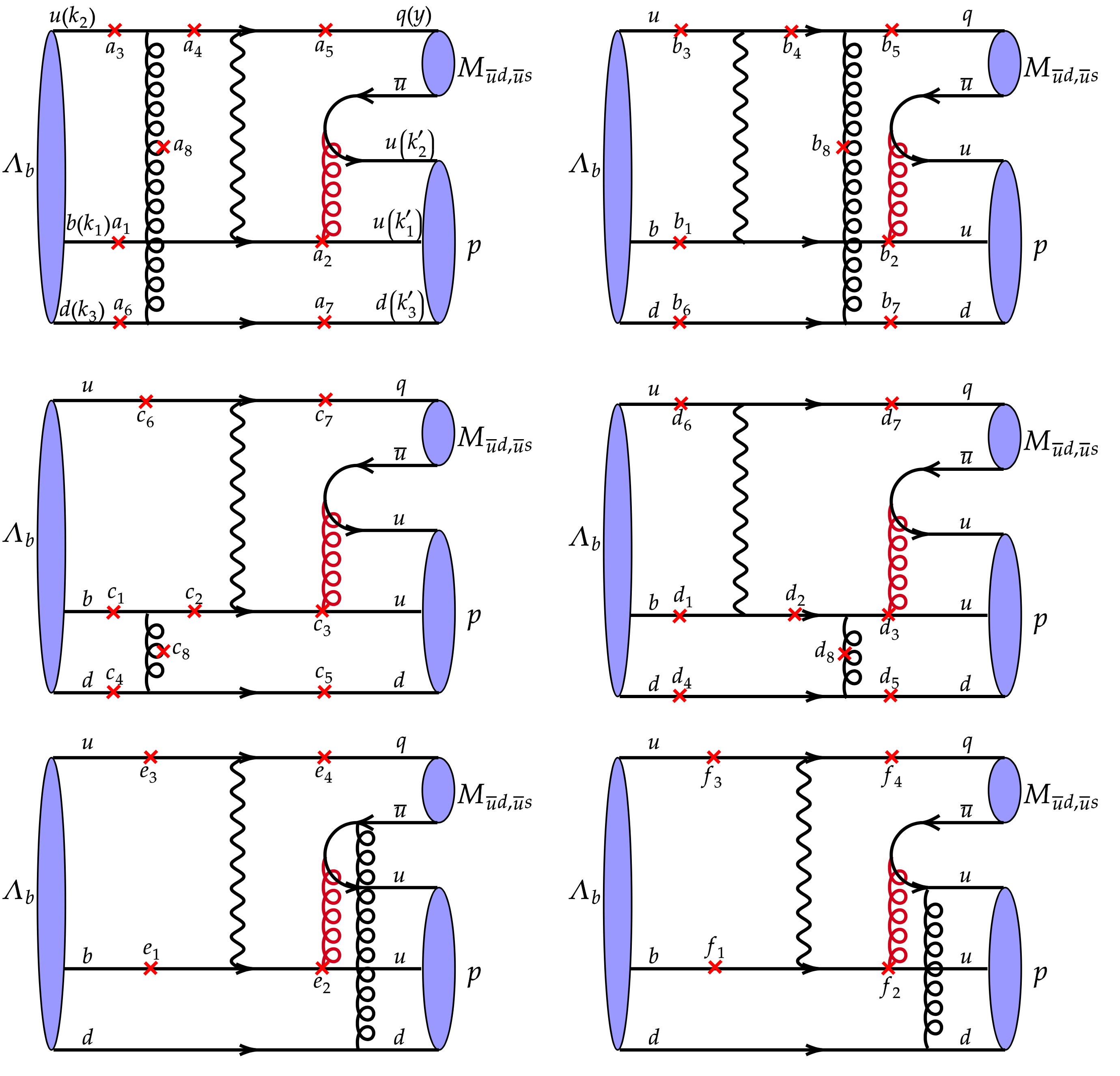
Figure 17: Feynman diagrams contributing to the $E_{2}$ topology.

The functions

$$\begin{split}M_{E_{2}(a4)}=&\frac{G_{F}}{\sqrt{2}}\left\{V_{ub}V_{uq}^{\ast}\left[f_{1}C_{1}+f_{2}C_{2}\right]\right\}M_{E_{2}(a4)}^{LL},\\ M_{P^{E_{1}^{u}}(a4)}=&-\frac{G_{F}}{\sqrt{2}}\left\{V_{tb}V_{tq}^{\ast}\left[f_{1}C_{3}+f_{2}C_{4}+f_{1}C_{9}+f_{2}C_{10}\right]\right\}M_{E_{2}(a4)}^{LL}\\ &-\frac{G_{F}}{\sqrt{2}}\left\{V_{tb}V_{tq}^{\ast}\left[-2f_{1}C_{5}-2f_{2}C_{6}-2f_{1}C_{7}-2f_{2}C_{8}\right]\right\}M_{E_{2}(a4)}^{SP},\end{split}$$ (106)

involve the color factors $f_{1}=-8/3$ and $f_{2}=-16/3$, and the matrix elements

$$M_{E_{2}(a4)}^{LL}\equiv\langle ph|(\bar{u}b)_{V-A}(\bar{q}u)_{V-A}|\Lambda_{b}\rangle_{E_{2}}$$

$$= \Big{\{}8(-4m_{\Lambda_{b}}^{4}\psi_{4}T_{1}x_{3}^{\prime}(-1+x_{2}+x_{3}+y)\phi_{m}^{A}+m_{\Lambda_{b}}^{3}(2m_{p}x_{3}^{\prime}(\psi_{4}(P_{1}-S_{1}+T_{3}+T_{7})(x_{2}^{\prime}+x_{3}^{\prime})$$

$$+(\psi_{3}^{-+}+\psi_{3}^{+-})T_{2}(-1+x_{2}+x_{3}+y))\phi_{m}^{A}+m_{0}(\psi_{3}^{-+}+\psi_{3}^{+-})(A_{1}-V_{1})(x_{2}+x_{3})(-1+x_{2}+x_{3}+y)$$

$$(\phi_{m}^{P}-\phi_{m}^{T}))+m_{0}m_{p}^{3}(\psi_{3}^{-+}+\psi_{3}^{+-})(A_{6}-V_{6})x_{3}^{\prime}(x_{2}^{\prime}+x_{3}^{\prime})(\phi_{m}^{P}+\phi_{m}^{T})+m_{0}m_{p}^{2}m_{\Lambda_{b}}(A_{4}(\psi_{3}^{-+}+\psi_{3}^{+-})x_{3}^{\prime}$$

$$(-1+x_{2}+x_{3}+y)(\phi_{m}^{P}-\phi_{m}^{T})+\psi_{3}^{-+}V_{4}x_{3}^{\prime}(-1+x_{2}+x_{3}+y)(\phi_{m}^{P}-\phi_{m}^{T})+\psi_{3}^{+-}V_{4}x_{3}^{\prime}(-1+x_{2}+x_{3}+y)$$

$$(\phi_{m}^{P}-\phi_{m}^{T})+2A_{4}\psi_{2}(x_{2}+x_{3})(x_{2}^{\prime}+x_{3}^{\prime})(\phi_{m}^{P}+\phi_{m}^{T})-2\psi_{2}V_{4}(x_{2}+x_{3})(x_{2}^{\prime}+x_{3}^{\prime})(\phi_{m}^{P}+\phi_{m}^{T})$$

$$-2\psi_{4}(A_{5}+V_{5})x_{3}^{\prime}(x_{2}^{\prime}+x_{3}^{\prime})(\phi_{m}^{P}+\phi_{m}^{T}))+m_{p}m_{\Lambda_{b}}^{2}(-m_{p}(\psi_{3}^{-+}+\psi_{3}^{+-})(P_{2}+S_{2}+T_{4}-T_{8})x_{3}^{\prime}(x_{2}^{\prime}+x_{3}^{\prime})\phi_{m}^{A}$$

$$-2m_{0}\psi_{2}(A_{2}+V_{2})(-1+x_{2})x_{2}\phi_{m}^{P}+m_{0}(A_{3}(\psi_{3}^{-+}(x_{2}+x_{3})(x_{2}^{\prime}+x_{3}^{\prime})+\psi_{3}^{+-}(x_{2}+x_{3})(x_{2}^{\prime}+x_{3}^{\prime})$$

$$+2\psi_{4}x_{3}^{\prime}(-1+x_{2}+x_{3}+y))\phi_{m}^{P}+(2\psi_{2}(A_{2}+V_{2})x_{3}+\psi_{3}^{+-}V_{3}(x_{2}+x_{3})(x_{2}^{\prime}+x_{3}^{\prime})$$

$$-2(\psi_{4}V_{3}x_{3}^{\prime}(-1+x_{2}+x_{3}+y)+\psi_{2}V_{2}(x_{3}(2x_{2}+x_{3})+(x_{2}+x_{3})y)$$

$$+A_{2}\psi_{2}(x_{3}(x_{3}+y)+x_{2}(2x_{3}+y))))\phi_{m}^{P}+A_{3}(\psi_{3}^{-+}(x_{2}+x_{3})(x_{2}^{\prime}+x_{3}^{\prime})+\psi_{3}^{+-}(x_{2}+x_{3})(x_{2}^{\prime}+x_{3}^{\prime})$$

$$-2\psi_{4}x_{3}^{\prime}(-1+x_{2}+x_{3}+y))\phi_{m}^{T}+(\psi_{3}^{+-}V_{3}(x_{2}+x_{3})(x_{2}^{\prime}+x_{3}^{\prime})+2A_{2}\psi_{2}(x_{2}+x_{3})(-1+x_{2}+x_{3}+y)$$

$$+2\psi_{2}V_{2}(x_{2}+x_{3})(-1+x_{2}+x_{3}+y)+2\psi_{4}V_{3}x_{3}^{\prime}(-1+x_{2}+x_{3}+y))\phi_{m}^{T}$$

$$+\psi_{3}^{-+}V_{3}(x_{2}+x_{3})(x_{2}^{\prime}+x_{3}^{\prime})(\phi_{m}^{P}+\phi_{m}^{T}))))\Big{\}}$$

$$+\Big{\{}-8(4m_{\Lambda_{b}}^{4}\psi_{4}T_{1}x_{3}^{\prime}(-1+x_{2}+x_{3}+y)\phi_{m}^{A}+m_{\Lambda_{b}}^{3}(2m_{p}x_{3}^{\prime}(\psi_{4}(P_{1}-S_{1}+T_{3}+T_{7})(x_{2}^{\prime}+x_{3}^{\prime})$$

$$-(\psi_{3}^{-+}+\psi_{3}^{+-})T_{2}(-1+x_{2}+x_{3}+y))\phi_{m}^{A}-m_{0}(\psi_{3}^{-+}+\psi_{3}^{+-})(A_{1}-V_{1})(x_{2}+x_{3})(-1+x_{2}+x_{3}+y)$$

$$(\phi_{m}^{P}-\phi_{m}^{T}))+m_{0}m_{p}^{3}(\psi_{3}^{-+}+\psi_{3}^{+-})(A_{6}-V_{6})x_{3}^{\prime}(x_{2}^{\prime}+x_{3}^{\prime})(\phi_{m}^{P}+\phi_{m}^{T})+m_{0}m_{p}^{2}m_{\Lambda_{b}}(-A_{4}(\psi_{3}^{-+}+\psi_{3}^{+-})x_{3}^{\prime}$$

$$(-1+x_{2}+x_{3}+y)(\phi_{m}^{P}-\phi_{m}^{T})-\psi_{3}^{-+}V_{4}x_{3}^{\prime}(-1+x_{2}+x_{3}+y)(\phi_{m}^{P}-\phi_{m}^{T})-\psi_{3}^{+-}V_{4}x_{3}^{\prime}(-1+x_{2}+x_{3}+y)$$

$$(\phi_{m}^{P}-\phi_{m}^{T})+2A_{4}\psi_{2}(x_{2}+x_{3})(x_{2}^{\prime}+x_{3}^{\prime})(\phi_{m}^{P}+\phi_{m}^{T})-2\psi_{2}V_{4}(x_{2}+x_{3})(x_{2}^{\prime}+x_{3}^{\prime})(\phi_{m}^{P}+\phi_{m}^{T})$$

$$-2\psi_{4}(A_{5}+V_{5})x_{3}^{\prime}(x_{2}^{\prime}+x_{3}^{\prime})(\phi_{m}^{P}+\phi_{m}^{T}))+m_{p}m_{\Lambda_{b}}^{2}(-m_{p}(\psi_{3}^{-+}+\psi_{3}^{+-})(P_{2}+S_{2}+T_{4}-T_{8})x_{3}^{\prime}(x_{2}^{\prime}+x_{3}^{\prime})\phi_{m}^{A}$$

$$+2m_{0}\psi_{2}(A_{2}+V_{2})(-1+x_{2})x_{2}\phi_{m}^{P}+m_{0}(A_{3}(\psi_{3}^{-+}(x_{2}+x_{3})(x_{2}^{\prime}+x_{3}^{\prime})+\psi_{3}^{+-}(x_{2}+x_{3})(x_{2}^{\prime}+x_{3}^{\prime})$$

$$-2\psi_{4}x_{3}^{\prime}(-1+x_{2}+x_{3}+y))\phi_{m}^{P}+(-2\psi_{2}(A_{2}+V_{2})x_{3}+\psi_{3}^{+-}V_{3}(x_{2}+x_{3})(x_{2}^{\prime}+x_{3}^{\prime})$$

$$+2(\psi_{4}V_{3}x_{3}^{\prime}(-1+x_{2}+x_{3}+y)+\psi_{2}V_{2}(x_{3}(2x_{2}+x_{3})+(x_{2}+x_{3})y)$$

$$+A_{2}\psi_{2}(x_{3}(x_{3}+y)+x_{2}(2x_{3}+y))))\phi_{m}^{P}+A_{3}(\psi_{3}^{-+}(x_{2}+x_{3})(x_{2}^{\prime}+x_{3}^{\prime})+\psi_{3}^{+-}(x_{2}+x_{3})(x_{2}^{\prime}+x_{3}^{\prime})$$

$$+2\psi_{4}x_{3}^{\prime}(-1+x_{2}+x_{3}+y))\phi_{m}^{T}+(\psi_{3}^{+-}V_{3}(x_{2}+x_{3})(x_{2}^{\prime}+x_{3}^{\prime})-2A_{2}\psi_{2}(x_{2}+x_{3})(-1+x_{2}+x_{3}+y)$$

$$-2\psi_{2}V_{2}(x_{2}+x_{3})(-1+x_{2}+x_{3}+y)-2\psi_{4}V_{3}x_{3}^{\prime}(-1+x_{2}+x_{3}+y))\phi_{m}^{T}$$

$$+\psi_{3}^{-+}V_{3}(x_{2}+x_{3})(x_{2}^{\prime}+x_{3}^{\prime})(\phi_{m}^{P}+\phi_{m}^{T}))))\Big{\}}\gamma_{5},$$ (107)