Spatial dynamics of flexible nano-swimmers under a rotating magnetic field

Abstract

Micro-nano-robotic swimmers have promising potential for future biomedical tasks such as targeted drug delivery and minimally-invasive diagnosis. An efficient method for controlled actuation of such nano-swimmers is applying a rotating external magnetic field, resulting in helical corkscrew-like locomotion. In previous joint work, we presented fabrication and actuation of a simple magnetic nano-swimmer composed of two nano-rods connected by a short elastic hinge. Experiments under different actuation frequencies result in different motion regimes. At low frequencies, in-plane tumbling; at higher frequencies, moving forward in a spatial helical path in synchrony with the rotating magnetic field; in further frequency increase, asynchronous swimming is obtained. In this work, we present mathematical analysis of this nano-swimmer motion. We consider a simple two-link model and explicitly formulate and analyze its nonlinear dynamic equations, and reduce them to a simpler time-invariant system. For the first time, we obtain explicit analytic solutions of synchronous motion under simplifying assumptions, for both solutions of in-plane tumbling and spatial helical swimming. We conduct stability analysis of the solutions, presenting stability transitions and bifurcations for the different solution branches. Furthermore, we present analysis of the influence of additional effects, as well as parametric optimization of the swimmer’s speed. The results of our theoretical study are essential for understanding the nonlinear dynamics of experimental magnetic nano-swimmers for biomedical applications, and conducting practical optimization of their performance.

I Introduction

Nano-swimmers are of great interest due to their promising potential for biomedical purposes, with applications ranging from internal sensing to targeted drug delivery and even carrying out medical procedures [1]. In order to understand how to create propulsion in the nanoscale dimensions, where motion is dominated by viscosity, one first needs to examine microorganisms’ motion. Microorganisms such as Salmonella, Helicobacter pylory, or Euglena gracilis are propelled by corkscrew motion of their tail [2], and theoretical models have been developed [3] to investigate their motion in the dominant viscosity regime. The model of a sphere with a tail shows two types of locomotion mechanisms. First, rotation of a helical propeller rigid tail creating corkscrew forward motion; second, planar undulation of a flexible tail creating a forward motion.
In order to fabricate an artificial nano-machine capable of achieving those two types of locomotion, there is a need for actuation. Internal actuation in this scale is not yet applicable mechanisms and would increase the manufacturing cost and complexity of the nanomachine. Thus, external actuation is an easier, practical solution. Using ultrasound, optic, electrical or magnetic forcing to create actuation torque were shown to be applicable [4, 5, 6].
The most common way is applying a time-varying external magnetic field while the nano-swimmer’s structure contains a magnetic part, resulting in application of a magentic torque actuating the swimmer. Experiments showed that applying a rotating magnetic field on rigid nano-helix with a magnetic heads creates forward locomotion [7, 8]. However, fabricating such chiral/helical three-dimensional structure in nanoscale is a long and delicate procedure [9]. In recent years, new kind of flexible nano-swimmers has been fabricated [10, 11], using rigid links connected by a short flexible hinge. Those nano-swimmers are much easier to manufacture. Actuated by a rotating magnetic field, it has been shown [10] that such nano-swimmers can also create spatial helical forward locomotion. Such magnetic nano-swimmers display different types of motion under different ranges of rotational frequencies of the magnetic field. At low-frequency, wobble in a plane without net swimming, and in higher frequencies swimming forward with spatial helical corkscrew motion [10]. At even higher frequencies, the nano-swimmer’s motion loses its synchronization with the magnetic field’s rotation, an effect named step-out [12].
In order to investigate these phenomena, there is a need to devise a simple mathematical model, which is amenable to explicit analysis. Some models have been developed for a single rigid body, starting from simple magnetic rigid ellipsoid under constant external torque [13], showing frequency-dependent stability transitions. Later, a model of a magnetic rigid chiral helix swimmer [14] shows frequency-dependent motion regimes, their stability, transitions, and step-out frequency for the loss of the synchronous motion.
For the flexible nano-swimmer under a rotating magnetic field, experimental results [15] followed by elastohydrodynamic model taking into account the elasticity of the nanowire and its hydrodynamic interaction with the fluid medium [16], considered a model with a rigid head and a flexible tail nano-swimmer, showing spatial motion with agreement to the theoretical model. Recent work [17] presents a multiple bead-spring model, allowing for arbitrary filament geometry and flexibility, and taking into account hydrodynamic interactions. This numerical work of multiple degrees-of-freedom (DOF) model also showed the motion dependence on frequency. In the case of a planar oscillating magnetic field, the work [18] proposed a simple two-link model with a passive revolute joint acted by torsion spring under a planar oscillating magnetic field. Using this simple model allows finding analytically the motion’s dependence on the oscillation frequency, including optimal swimming speed, as well as stability transitions [19] and bifurcations [20]. For the case of a rotating magnetic field, the recent work [21] considered the same two-link model in order to study the behavior of the experimental nano-swimmer, and showed, by numerical simulations, the frequency-dependent motion regimes. However, an analytical investigation of the solution regimes, stability analysis, and performance optimization has not been done in [21].

The goal of this work is to complement the numerical simulations in [21] by presenting full analytical treatment of the two-link model dynamics. We obtain explicit expressions for the frequency-dependent solutions and their transitions, and conduct numerical optimization of the nano-swimmer’s performance with respect to various parameters.

II Problem formulation

We now present the two-link model and formulation of its dynamic equations of motion, as derived previously in [21].

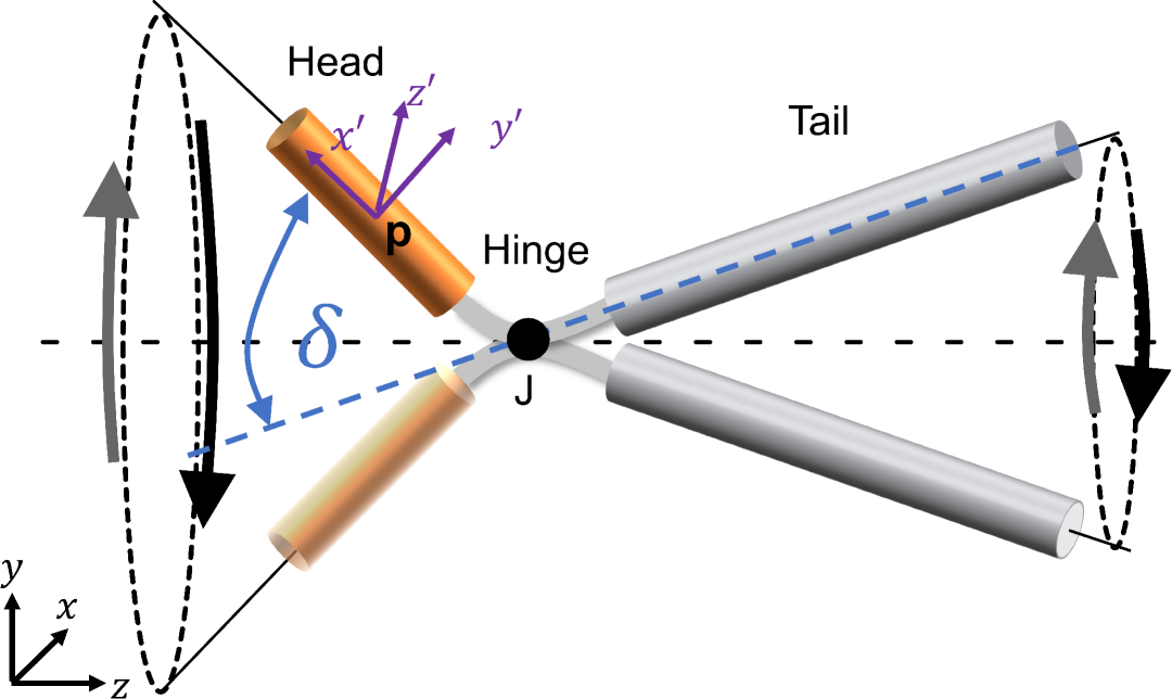
Figure 1: Schematic sketch of the two-link nano-swimmer model. p is the center of the head link, J is the pointed revolute joint point that connects the head and tail link. The joint’s axis of rotation is $\mathbf{{z^{\prime}}}$, whereas the swimmers’ links lie within $\mathbf{{x^{\prime}}}-\mathbf{{y^{\prime}}}$ plane.

The nano-swimmer’s simplified model from [21], as shown in Fig. 1, consists of two rigid links: the magnetic link, named “head” and the nonmagnetic link, named “tail”. A short thin nano-wire connects them, acting as a flexible hinge. The nano-swimmer moves in a 3D environment, where the position of the head link’s center is denoted by coordinates $x,y,z$. In order to describe its orientation, we assign a moving reference frame $\{\hat{\mathbf{{x}}}^{\prime},\hat{\mathbf{{y}}}^{\prime},\hat{\mathbf{{z}}}^{\prime}\}$ fixed to the center of the head link, whose orientation with respect to the world frame is parametrized by three Euler angles $\phi,\theta,\psi$. The short flexible hinge is represented by a pointed uniaxial revolute joint along a common normal to the longitudinal axes of the head and tail links, which are assumed to lie on a common plane. The relative angle of this joint is denoted by $\delta$, as shown in Figure 1. The nano-swimmer’s motion is described by a vector of 7 coordinates, $\mathbf{{q}}=(x,y,z,\phi,\theta,\psi,\delta)^{T}$. The matrix describing the orientation of the rotating reference frame fixed to the head $\{\hat{\mathbf{{x}}}^{\prime},\hat{\mathbf{{y}}}^{\prime},\hat{\mathbf{{z}}}^{\prime}\}$ with respect to the world reference frame $\{\hat{\mathbf{{x}}},\hat{\mathbf{{y}}},\hat{\mathbf{{z}}}\}$, is obtained as the product of three extrinsic rotation matrices according to the Euler ZXZ convention as $\mathbf{{R}}_{1}=\mathbf{{R}}_{\phi}\mathbf{{R}}_{\theta}\mathbf{{R}}_{\psi}$.

$$\mathbf{{R}}_{1}=\left(\begin{array}[]{ccc}C_{\phi}\,C_{\psi}\text{-}C_{\theta}\,S_{\phi}\,S_{\psi}&\text{-}C_{\phi}\,S_{\psi}\text{-}C_{\psi}\,C_{\theta}\,S_{\phi}&S_{\phi}\,S_{\theta}\\ C_{\psi}\,S_{\phi}\text{+}C_{\phi}\,C_{\theta}\,S_{\psi}&C_{\phi}\,C_{\psi}\,C_{\theta}\text{-}S_{\phi}\,S_{\psi}&\text{-}C_{\phi}\,S_{\theta}\\ S_{\psi}\,S_{\theta}&C_{\psi}\,S_{\theta}&C_{\theta}\end{array}\right),$$ (4)

where $C_{\phi}\!=\!\cos\phi,C_{\psi}\!=\!\cos\psi,C_{\theta}\!=\!\cos\theta,S_{\phi}\!=\!\sin\phi,S_{\psi}\!=\!\sin\psi,S_{\theta}\!=\!\sin\theta$. In order to have a unique description for each orientation, we define the ranges of Euler angles as: $-\pi\leq\phi<\pi$, $0<\theta\leq\pi$, and $0\leq\psi<2\pi$.
In order to formulate the dynamics of the system, we now describe the forces and torques acting on the nano-swimmer. First, we consider the hydrodynamic forces and torques. Assuming Stokes flow and neglecting hydrodynamic interaction between the links, the drag force and torque acting upon each link can be expressed as:

$$\mathbf{{\textbf{{f}}}}^{h}_{i}=-c_{t}^{i}(\mathbf{{v}}_{i}\cdot\hat{\mathbf{{t}}}_{i})\hat{\mathbf{{t}}}_{i}-c_{n}^{i}(\mathbf{{v}}_{i}-(\mathbf{{v}}_{i}\cdot\hat{\mathbf{{t}}}_{1})\hat{\mathbf{{t}}}_{i})=$$ (5)

$$\left((c_{n}^{i}-c_{t}^{i})l_{i}\hat{\mathbf{{t}}}_{i}\cdot\hat{\mathbf{{t}}}_{i}^{T}-c_{n}^{i}\mathbf{{I}}_{3x3}\right)\mathbf{{v}}_{i}$$

$$\mathbf{{\tau}}^{h}_{i}=-d_{t}^{i}(\mathbf{{\omega}}_{i}\cdot\hat{\mathbf{{t}}}_{i})\hat{\mathbf{{t}}}_{i}-d_{n}^{i}(\mathbf{{\omega}}_{i}-(\mathbf{{v}}_{i}\cdot\hat{\mathbf{{t}}}_{1})\hat{\mathbf{{t}}}_{i})=$$ (6)

$$\left((d_{n}^{i}-d_{t}^{i})l_{i}\hat{\mathbf{{t}}}_{i}\cdot\hat{\mathbf{{t}}}_{i}^{T}-c_{n}^{i}\mathbf{{I}}_{3x3}\right)\mathbf{{\omega}}_{i}$$

where $c_{n}^{i},c_{t}^{i},d_{n}^{i},d_{t}^{i}$ for $i=1,2$ are the linear and rotational drag coefficients along the normal and tangent to the longitudinal axis of the head and tail links. The swimmer’s links can be modeled as prolate spheroids or finite slender rods, where drag coefficients for prolate spheroid are given in [22, 23], and for finite slender rods in [24].
Next, we describe the magnetic effects on the nano-swimmer. It is assumed that the magnetization vector of the head link is directed along its longitudinal axis $\mathbf{{\hat{t}}}_{1}$ and has magnitude $m$. The external magnetic field is assumed to be spatially uniform and time varying, with rotating component in $x-y$ plane, and possibly an additional constant component in $\hat{\mathbf{{z}}}$ direction. (Note the differences from [21] in the choice of the plane of rotation, as well as the addition of constant component). That is, the magnetic field $\mathbf{{B}}(t)$ rotates along the surface of a cone, and is formulated as:

$$\mathbf{{B}}(t)=b(\sin(\Omega t)\hat{\mathbf{{x}}}+\cos(\Omega t)\hat{\mathbf{{y}}}+h\hat{\mathbf{{z}}})$$ (7)

The torque acting on the head link due to the rotating magnetic field is:

$$\bm{\tau}_{m}=m(\mathbf{{\hat{t}}}_{1}\times\mathbf{{B}}(t))$$ (8)

Lastly, we consider the nano-swimmer’s elasticity. The short flexible wire connecting the head and tail link is modeled as a pointed uni-axial joint with torsion spring, applying torque:

$$\tau_{k}=-k\delta$$ (9)

Due to the negligibility of inertial effects in Stokes flow, the swimmer is always in force and torque balance. Using kinematic relations (see detailed derivation in [21, 25]), one can write the balance equations and derive the nano-swimmer’s dynamic equations of motion in the form of:

$$\mathbf{{A}}(\mathbf{{q}})\mathbf{{\dot{q}}}=\mathbf{{b}}(\mathbf{{q}},t)$$ (10)

This gives a time-dependent system of 7 coupled nonlinear ordinary differential equations in $\mathbf{{q}}(t)$, which can be integrated numerically.

III Numerical Simulations

In this section, we present numerical simulations representing the nano-swimmer’s dynamics. We use the following physical values of parameters from [21]:

$$\begin{split}&k=3.25\times 10^{-17}[N\cdot m],b=15[mT],m=9000[A/m]\\ &l_{1}=l_{2}=7.2[\mu m],\mu=0.0124[N\cdot s/m^{2}]\end{split}$$ (11)

We integrate the equations of motion (10) using Matlab’s $ode45$ function, assuming purely rotating magnetic field with $h=0$, and using spheroid drag coefficients from [22, 23]. In all simulations, we consider initial conditions of orientation angles $\phi(0)=\psi(0)=0,\theta(0)=1\;[rad]$ and joint angle $\delta(0)=2\;[rad]$. By integrating in a wide range of actuation frequencies $\Omega[rad/sec]$, one obtains three different types of motion: in low frequencies, planar tumbling - rigid rotation of the nano-swimmer in $x-y$ plane, in synchrony with the rotating magnetic field, as shown in Figure 2.

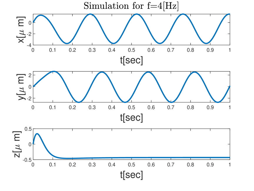
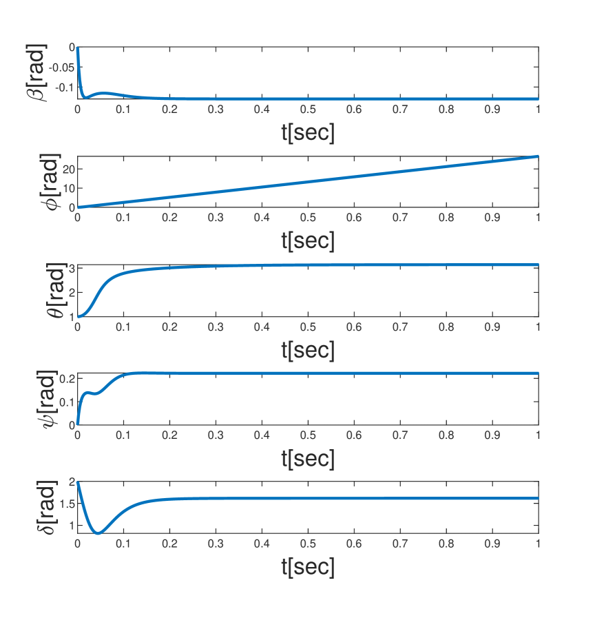
Figure 2: Numerical simulations under rotating magnetic field of f$=\Omega/2\pi=4[Hz]$, giving planar tumbling motion in $x-y$ plane.

After an initial transient, the angles $\theta(t),\psi(t),\delta(t)$ converge to constant steady-state values, whereas $\phi(t)$ grows linearly with time $t$. In translational motion, $x(t)$ and $y(t)$ undergo periodic oscillations around zero, after a small initial transient, while $z(t)$ stays constant, resulting in zero net propulsion. In higher frequencies, the nano-swimmer‘s body gets out of the $x-y$ plane and moves in a spatial corkscrew-like motion, following a helical path. After an initial transient, the steady-state motion is also synchronous with the applied magnetic field, as shown in Figure 3.

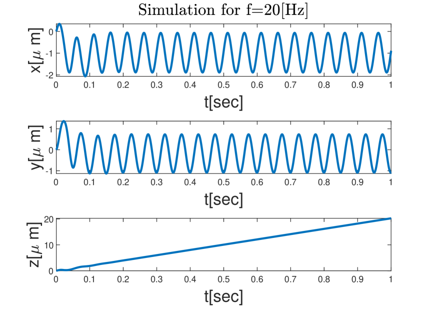
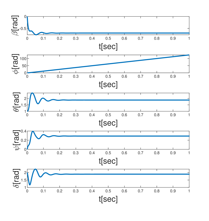
Figure 3: Numerical simulations under rotating magnetic field of f$=\Omega/2\pi=20[Hz]$, giving synchronous motion of spatial helical trajectory.

One can see that the three angles $\theta(t),\psi(t),\delta(t)$ behave similarly to the previous case, and reach constant values after an initial transient. In the translational motion, $x(t),y(t)$ are also oscillating about constant values, but $z(t)$ grows linearly in time, giving nonzero net propulsion along $\mathbf{{\hat{z}}}$ direction in constant speed.
In higher frequencies as shown in Figure 4, the nano-swimmer’s motion loses its synchronization with the applied magnetic field, an effect known as “step-out” [26], the nano-swimmer continues moving forward in an asynchronous motion in all 7 coordinates.

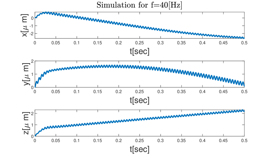
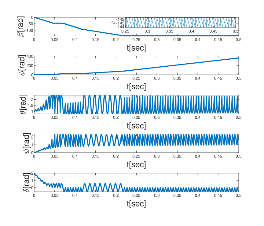
Figure 4: Numerical simulations under rotating magnetic field of f$=\Omega/2\pi=40[Hz]$, resulting in asynchronous motion.

In Figure 5 we present the mean forward speed of the nano-swimmer in $\hat{\mathbf{{z}}}$ direction, denoted by $V_{z}$, as a function of frequency $\Omega$ across the three different motion regimes.

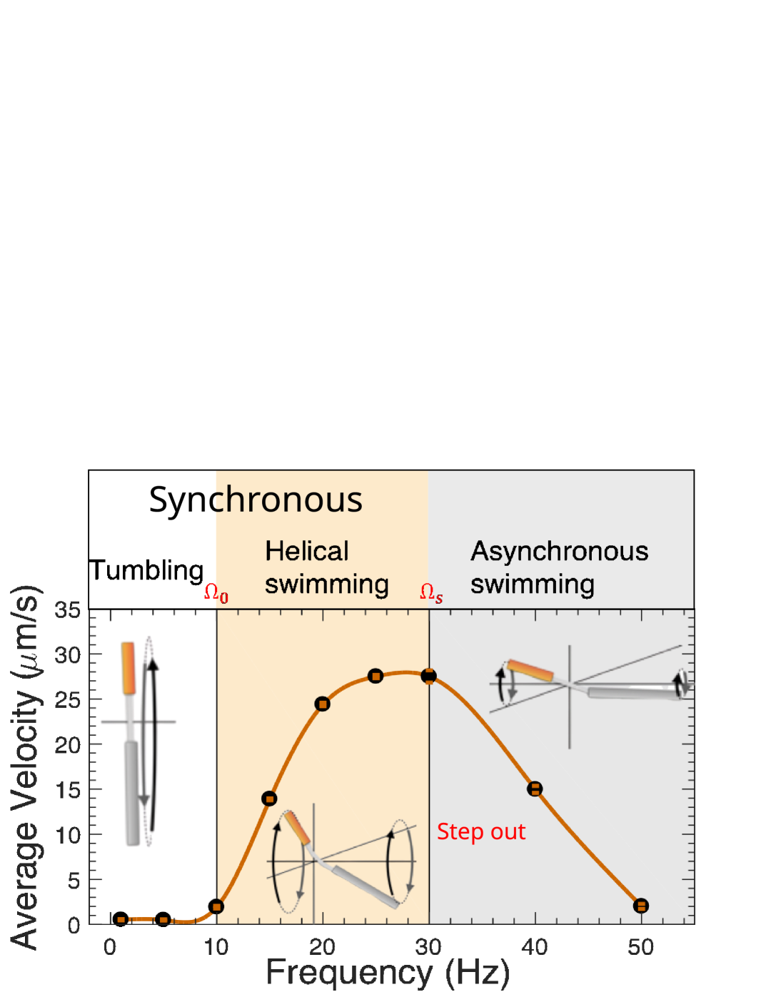
Figure 5: The average swimminbg speed $V_{z}$ as function of frequency. Solid line - calculated from numerical simulations; black dots are from experimental data [21].

The mean speed changes smoothly as a function of the frequency. In the low frequency range of planar tumbling motion, the mean speed is zero. In higher frequencies, in the regime of spatial helical motion, the nano-swimmer leaves the $x-y$ plane and starts a corkscrew locomotion. We define the critical frequency where the swimmer leaves the $\mathbf{{\hat{x}\mathbf{{\hat{y}}}}}$ plane as $\Omega_{0}$. Increasing the frequency above $\Omega_{0}$, one can see an increase in the speed $V_{z}$ up to a maximum. Further increasing the frequency, the speed continues to decrease. Upon further increase of frequency, the swimmer’s motions switch to the asynchronous swimming, where the switching frequency is denoted by $\Omega_{s}$, also known as the step-out frequency [12, 26].

IV Analysis

We now present analytical investigation of the two-link nano-swimmer dynamics. First, we reduce the equations of motion and make some simplifying assumptions that further reduce the number of parameters and simplify the equations. Then we study synchronous solutions, their bifurcations and stability transitions.

IV.1 Reducing the Equations of Motion

In order to investigate the system’s dynamic equations analytically, we now reduce the equations to a more compact form. First, as shown in Figures 2,3, three of the coordinates $\theta,\psi,\delta$ are constant in steady state synchronous motion, but $\phi$ is not. Since $\phi$ maintains constant phase shift from the magnetic field orientation $\Omega t$, following [14], we define a new coordinate of phase shift $\beta=\phi-\Omega t$ which in steady state is also constant, as shown in Figures 2 and 3. Using the new coordinates vector: $\tilde{\mathbf{{q}}}=(x,y,z,\beta,\theta,\psi,\delta)^{T}$, the system’s equations of motion (10) are obtained as:

$$\tilde{\mathbf{{A}}}(\tilde{\mathbf{{q}}})\dot{\tilde{\mathbf{{q}}}}=\tilde{\mathbf{{b}}}(\tilde{\mathbf{{q}}})$$ (12)

Importantly, this new system is now time-invariant, and in the synchronous steady state, four coordinates converge to constant values, implying that it is an equilibrium state for those coordinates: $\dot{\theta}=\dot{\beta}=\dot{\psi}=\dot{\delta}=0$. In Figures 2,3, the numerical simulations results for the coordinate $\phi$ and the coordinate $\beta=\phi-\Omega t$ are presented. One can see that $\beta(t)$ in both cases converges to constant values in steady state, after a transient response.
In order to further reduce the system’s dynamic equations, we decompose the coordinates $\tilde{\mathbf{{q}}}$ into displacement part $\mathbf{{q}}_{d}$ and angular part$,\mathbf{{q}}_{a}$ as:

$$\tilde{\mathbf{{q}}}=\left(\mathbf{{q}}_{d},\mathbf{{q}}_{a}\right)^{T},\mathbf{{q}}_{d}=\left(x,y,z\right)^{T},\mathbf{{q}}_{a}=\left(\beta,\theta,\psi,\delta\right)^{T}$$ (13)

Then, we decompose the matrices $\mathbf{{\tilde{A},\tilde{b}}}$ from (12) into blocks as:

$$\underbrace{\left(\begin{matrix}\mathbf{{A}}_{dd}&\mathbf{{A}}_{da}\\ \mathbf{{A}}_{ad}&\mathbf{{A}}_{aa}\end{matrix}\right)}_{\mathbf{{\tilde{A}}}(\mathbf{{q}}_{a})}\left(\begin{matrix}\mathbf{{\dot{q}}}_{d}\\ \mathbf{{\dot{q}}}_{a}\end{matrix}\right)=\underbrace{\left(\begin{matrix}\mathbf{{0}}\\ \mathbf{{g}}\end{matrix}\right)}_{\mathbf{{\tilde{b}}}(\mathbf{{q}}_{a})}$$ (14)

Note that equations (14) depend only on the angles $\mathbf{{q}}_{a}$ due to translational invariance. The translational velocity vector $\mathbf{{\dot{q}}}_{d}$ can thus be extracted from (14) as:

$$\dot{\mathbf{{q}}}_{d}=-(\mathbf{{A}}_{dd})^{-1}\mathbf{{A}}_{da}\dot{\mathbf{{q}}}_{a}$$ (15)

By substituting (15) to (14), one obtains:

$$\underbrace{\left(\mathbf{{A}}_{ad}\left(-(\mathbf{{A}}_{dd})^{-1}\mathbf{{A}}_{da}\right)+\mathbf{{A}}_{aa}\right)}_{\mathbf{{A^{\prime}}}(\mathbf{{q}}_{a})}\dot{\mathbf{{q}}}_{a}=\mathbf{{g}}(\mathbf{{q}}_{a})$$ (16)

Thus, the system is reduced to a 4-DOF time-invariant system in $\mathbf{{q}}_{a}$ only. Assuming $\mathbf{{A^{\prime}}}$ is an invertible matrix, one can solve the equilibrium equation $\mathbf{{\dot{q}}}_{a}=0$ from the right side of equation (16) as:

$$\mathbf{{g}}(\mathbf{{q}}_{a})=\mathbf{{0}}$$ (17)

Solutions $\mathbf{{q}}_{a}=\mathbf{{q}}_{e}$ of equation (17) correspond to steady-state synchronous motion.

IV.2 Simplifying Assumptions and Scaling

The dynamic equations (16) depend on 15 physical constants, which calls for simplifications and reduction. We now apply the following simplifying assumptions in order to reduce the number of parameters. First, we assume a planar magnetic field with no $\hat{\mathbf{{z}}}$ component, $h=0$ in (7). Second, we consider equal links’ lengths $l_{1}=l_{2}=l$. (These two assumptions are relaxed later in Section V). Third, drag coefficients are simplified, assuming slender prolate spheroids according to [22, 23]. We use the following assumptions to reduce the number of drag coefficients. The translational coefficients are approximated as $c_{t}\approx\frac{1}{2}c_{n}$. For the rotational drag coefficients, since slender bodies satisfy $d_{t}\ll d_{n}$, we neglect it and assume $d_{t}=0$. We also take $d_{n}=c_{n}l^{2}/12$. These simplifications are fairly accurate approximation for slender spheroids [22, 23].

Non-dimensional equations: First, we define $l$ as the characteristic length. Next, we define two characteristic time scales, $t_{m}$ the magnetic characteristic time and $t_{k}$ the stiffness characteristic time:

$$t_{m}=\frac{c_{t}l^{2}}{bm},t_{k}=\frac{c_{t}l^{2}}{k},$$ (18)

Follwoing [18], the ratio between these two time scales is defined as the nondimensional parameter $\alpha=t_{m}/t_{k}=k/bm$.
We scale the time in (16) by the magnetic characteristic time $t_{m}$, and define the nondimensional frequency $\omega=\Omega t_{m}$. The scaled and reduced dynamic equations now have the form:

$$\mathbf{{A^{\prime}}}(\mathbf{{q}}_{a})\mathbf{{\dot{q}}}_{a}=\mathbf{{g}}(\mathbf{{q}}_{a})$$ (19)

Where “dot” now represents derivative with respect to the scaled time $t/t_{m}$. The matrix $\mathbf{{A^{\prime}}}(\mathbf{{q}}_{a})$ in (19) is given in Table 1, where $S_{\gamma}$ and $C_{\gamma}$ are shorthand notations for $\sin(\gamma)$ and $\cos(\gamma)$, respectively, for all angles $\gamma$.

$$\mathbf{{A^{\prime}}}(\mathbf{{q}}_{a})=\left(\begin{array}[]{cccc}\frac{1}{24}\left(5C_{\psi}+3S_{\delta}S_{\psi}-5c^{2}_{\delta}C_{\psi}+5C_{\delta}S_{\delta}S_{\psi}\right)&-\frac{S_{\theta}}{24}\left(3C_{\psi}S_{\delta}-5S_{\psi}+5C_{\delta}^{2}S_{\psi}+5C_{\delta}C_{\psi}S_{\delta}\right)&0&0\\ \frac{1}{12}\left(3S_{\delta-\psi}-5S_{2\delta+\psi}-9S_{\delta+\psi}-15S_{\psi}\right)&\frac{1}{48}S_{\theta}\left(9C_{\delta+\psi}+15C_{\psi}+3C_{\delta-\psi}+5C_{2\delta+\psi}\right)&0&0\\ 0&\frac{C_{\theta}(3+3C_{\delta})}{3(3-C_{\delta})}&\frac{3+C_{\delta}}{3(3-C_{\delta})}&\frac{3+C_{\delta}}{6(3-C_{\delta})}\\ 0&\frac{C_{\theta}(3+C_{\delta})}{6(3-C_{\delta})}&\frac{3+C_{\delta}}{6(3-C_{\delta})}&\frac{9+c^{2}_{\delta}}{6(9-c^{2}_{\delta})}\end{array}\right)$$

Table 1: The matrix $\mathbf{{A^{\prime}}}(\mathbf{{q}}_{a})$

The vector $\mathbf{{g}}(\mathbf{{q}}_{a})$ is given as:

$$\mathbf{{g}}(\mathbf{{q}}_{a})=\left(\begin{split}&\omega\sin\theta\sin\delta\left(a_{1}(\delta)\sin(\psi)+b_{1}(\delta)\cos(\psi)\right)\\ &\sin\theta\left(\sin\beta+\omega b_{2}(\delta)\cos(\psi)+a_{2}(\delta)\sin(\psi)\right)\\ &\cos\beta\sin\psi+\cos\theta\left(\sin\beta\cos\psi+\omega a_{3}(\delta)\right)\\ &\alpha\delta-\omega\cos\theta a_{4}(\delta)\end{split}\right)$$ (20)

where

$$\begin{split}&a_{1}(\delta)=-\frac{5}{3}\sin(\delta)\\ &b_{1}(\delta)=\frac{5}{3}\cos(\delta)+1\\ &a_{2}(\delta)=-\frac{1}{4}\sin(\delta)\left(1+\frac{5}{3}\cos(\delta)\right)\\ &b_{2}(\delta)=\frac{1}{4}\left(\frac{5}{3}+\cos(\delta)\left(2+\frac{5}{3}\cos(\delta)\right)\right)\\ &a_{3}(\delta)=\frac{6+\cos(\delta)\left(4+\frac{1}{3}\cos(\delta)\right)}{9-\cos^{2}(\delta)}\\ &a_{4}(\delta)=-\frac{1}{2}a_{3}(\delta)\end{split}$$ (21)

Equation (20) reached a compact simplified form, which enables solving the equilibrium equations (17). Note that this solution hold only if the matrix $\mathbf{{A^{\prime}}}(\mathbf{{q}}_{a})$ in (19) is invertible. From Table 1, the determinant of $\mathbf{{A^{\prime}}}(\mathbf{{q}}_{a})$ can be obtained as $\mathrm{det}(\mathbf{{A^{\prime}}}(\mathbf{{q}}_{a}))=\frac{1}{1296}S^{2}_{\delta}S_{\theta}$. One case of singularity of $\mathbf{{A^{\prime}}}(\mathbf{{q}}_{a})$ is $\sin(\delta)=0$. This configuration describes the cases where the two-links are aligned $\mathbf{{\hat{t}}}_{1}||\mathbf{{\hat{t}}}_{2}$. The physical reason for this singularity is our simplifying assumption that $d_{t}^{i}=0$, which means that there is no drag resistance for rotation about the links’ longitudinal direction. When $d_{t}\neq 0$, this singularity of $\mathbf{{A^{\prime}}}$ at $\sin(\delta)=0$ is removed. Nonetheless, we choose here to keep the simplifying assumption of $d_{t}=0$, since the case of $\sin(\delta)=0$ is anyway not an equilibrium solution of (20) for $\omega\neq 0$. The second case of singularity of $\mathbf{{A^{\prime}}}(\mathbf{{q}}_{a})$ is $\sin(\theta)=0$. This is associated with the swimmer lying in the $x-y$ plane - the planar tumbling motion, as discussed below.

IV.3 Planar Tumbling Solution

We now solve the equilibrium equations (17) for planar tumbling motion. The equilibrium values of $\mathbf{{q}}_{a}$ will be denoted by $\mathbf{{q}}_{e}=(\beta_{e},\theta_{e},\psi_{e},\delta_{e})$. Looking at the first two terms in (20), one can easily observe that they both vanish for $\sin(\theta_{e})=0$, meaning a planar solution.

$$\sin\theta_{e}=0\rightarrow\theta_{e}=\pi$$ (22)

By substituting this solution into the other terms in (20) and equating to zero, one obtains:

$$\cos\beta_{e}\sin\psi_{e}-\left(\sin\beta_{e}\cos\psi_{e}+\omega a_{3}(\delta_{e})\right)=0$$ (23)

$$\alpha\delta_{e}=-\omega a_{4}(\delta_{e})=\omega\frac{6+\cos(\delta_{e})\left(4+\frac{1}{3}\cos(\delta_{e})\right)}{2\left(9-\cos^{2}(\delta_{e}\right))}$$ (24)

Where $a_{3}(\delta_{e}),a_{4}(\delta_{e})$ are given in (21). Equation (24) is a scalar function in $\delta_{e},\omega$. For a given frequency $\omega$ one needs to solve a transcendental equation numerically for $\delta_{e}$. On the other hand, assuming given $\delta_{e}$ gives a simple analytical solution for $\omega$:

$$\omega=-\frac{\alpha\delta_{e}}{a_{4}(\delta_{e})}=\frac{2\alpha\delta_{e}\left(9-\cos^{2}(\delta_{e})\right)}{6+\cos(\delta_{e})\left(4+\frac{1}{3}\cos(\delta_{e})\right)}$$ (25)

In Figure 6 we present the solution for $\omega$ in the region of $\delta_{e}=[0,\pi]$.

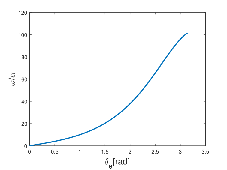
Figure 6: Nondimensional scaled frequency $\omega/\alpha$ as a function of equilibrium value of the link angle $\delta=\delta_{e}$ for the planar tumbling solution as obtained from (25).

We now proceed to solving the equilibrium values of the other angles $\psi,\beta$. Eq. (23) can be rewritten as:

$$\sin(\beta_{e}-\psi_{e})=\sin(\gamma_{e})=\omega a_{3}(\delta_{e})$$ (26)

This gives two solutions for $\gamma_{e}=\beta_{e}-\psi_{e}$ as a function of $\omega,\delta_{e}$. Note that for $\sin(\theta_{e})=0$, the first two terms in (20) vanish. Thus, one needs one more equation in order to find the angles $\beta_{e}$ and $\psi_{e}$ separately. This is resolved by considering the “full equilibrium equation” $\mathbf{{\dot{q}}}_{a}=\mathbf{{A^{\prime}}}^{-1}\mathbf{{g}}=\mathbf{{0}}$. Interestingly, the singularity of the matrix $\mathbf{{A^{\prime}}}$ for $\sin(\theta)=0$ is cancelled in the multiplication $\mathbf{{A^{\prime}}}^{-1}\mathbf{{g}}$, which becomes a well-defined finite vector. Substituting $\psi_{e}=\beta_{e}-\gamma_{e}$ into the second element of $\mathbf{{A^{\prime}}}^{-1}\mathbf{{g}}=0$ gives an equation where the only unknown is $\beta_{e}$:

$$f_{1}\sin(\beta_{e})^{2}+f_{2}\sin(\beta_{e})\cos(\beta_{e})+f_{3}=0,$$ (27)

where:

$$f_{1}=15\alpha\cos(\gamma_{e})\sin(\delta_{e})\cos(\delta_{e})-15\alpha\sin(\gamma_{e})\cos(\delta_{e})^{2}$$

$$+15\alpha\sin(\gamma_{e})+9\alpha\cos(\gamma_{e})\sin(\delta_{e})$$ (28)

$$f_{2}=15\alpha\cos(\gamma_{e})-15\alpha\sin(\delta_{e})\sin(\gamma_{e})\cos(\delta_{e})$$ (29)

$$-15\alpha\cos(\gamma_{e})\cos(\delta_{e})^{2}-9\alpha\sin(\delta_{e})\sin(\gamma_{e})$$

$$f_{3}=4\omega-4\omega\cos(\delta_{e})^{2}$$ (30)

Since $\gamma_{e}$ is already solved in (26) as a function of $\delta_{e},\omega$, equation (27) is solved as:

$$\begin{split}\beta_{e}=\arctan\left(\frac{(\pm f_{2}^{2}\mp\sqrt{f_{2}^{4}-4f_{2}^{2}f_{3}(f_{1}+f_{3}})f_{4}}{\pm f_{2}f_{3}f_{4}}\right)\end{split}$$ (31)

Where

$$f_{4}=\sqrt{\frac{f_{2}^{2}-2f_{1}f_{3}\pm\sqrt{f_{2}^{4}-4f_{2}^{2}f_{3}(f_{1}+f_{3})}}{f_{1}^{2}+f_{2}^{2}}}$$ (32)

We obtain four different solution pairs $(\beta_{e},\psi_{e})$ for every choice of $\delta_{e},\theta_{e}$. Each of these solutions has additional conditions for its existence, defined by the following inequalities. From (26), one obtains:

$$|\omega a_{3}(\delta_{e})|\leq 1$$ (33)

From (31), one obtains:

$$f_{2}^{4}-4f_{2}^{2}f_{3}(f_{1}+f_{3})\geq 0$$ (34)

$$f_{4}(\omega,\delta_{e})\geq 0$$ (35)

Those inequalities impose conditions for existence of each solution branch of planar tumbling.

Stability analysis: We now examine the stability of steady-state solutions of planar tumbling using linear analysis, by the Jacobian matrix, calculated analytically.

$$\mathbf{{J}}=\left.\frac{d\left[\mathbf{{A^{\prime}}}^{-1}\mathbf{{g}}\right]}{d\mathbf{{q}}}\right|_{\mathbf{{q}}=\mathbf{{q}}_{e}}=\begin{pmatrix}\sigma&\mathbf{{0}}\\ \mathbf{{0}}&\mathbf{{J_{m}}}\end{pmatrix}$$ (36)

For the planar tumbling solution, the resulting Jacobian matrix $\mathbf{{J}}$ has a block-diagonal structure as in (36). One eigenvalue of $\mathbf{{J}}$ is the diagonal term $\sigma$, given by:

$$\sigma=-\frac{1}{(4(\cos(\delta_{e})^{2}-1)}(3\alpha\sin(\beta_{e})(3\cos(\psi_{e})\sin(\delta_{e})$$

$$-5\sin(\psi_{e})+5\cos(\delta_{e})^{2}\sin(\psi_{e})+5\cos(\delta_{e})\cos(\psi_{e})\sin(\delta_{e})))$$ (37)

The three other eigenvalues $\mathbf{{J}}$ belong to the $3\times 3$ matrix block $\mathbf{{J_{m}}}$.The Jacobian’s expressions can be found at [25].
In order for the solution $\mathbf{{q}}_{e}$ to be a stable equilibrium, all eigenvalues of $\mathbf{{J}}$ are required to have negative real parts, $Re(\lambda_{i})<0$. Thus, a necessary condition for stability is $\sigma<0$. Figure 7 shows four solutions branches of $\beta_{e}$ angle, denoted by $\{a,b,c,d\}$, as a function of the nondimensional frequency $\omega$. Solid lines denote stable solutions, while dashed lines denote unstable ones. There is only one branch that has a stable part, solution {c} in the figure. This can be verified by Figure 8, which plots the maximal real part of eigenvalues of $\mathbf{{J}}$ as a function of nondimensional frequency $\omega$. For solution {c}, the eigenvalue that has the maximal real part is $\sigma$, and thus the sign of $\sigma$ determines its stability. One can find the critical value of $\delta_{e}$ corresponding to stability transition from solving $\sigma=0$ in (37) using the solution of $\psi_{e}(\delta_{e}),\beta_{e}(\delta_{e})$, and then use (25) to find the critical frequency $\omega_{0}$. This frequency corresponds to a bifurcation point where the spatial helical solution emerges, as we shall see below.

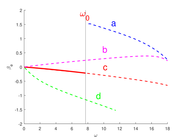
Figure 7: Multiple solutions branches of $\beta_{e}$ for planar tumbling, as a function of nondimensional frequency $\omega$. Solid/dashed curves deonte stable/unstable solutions, respectively.

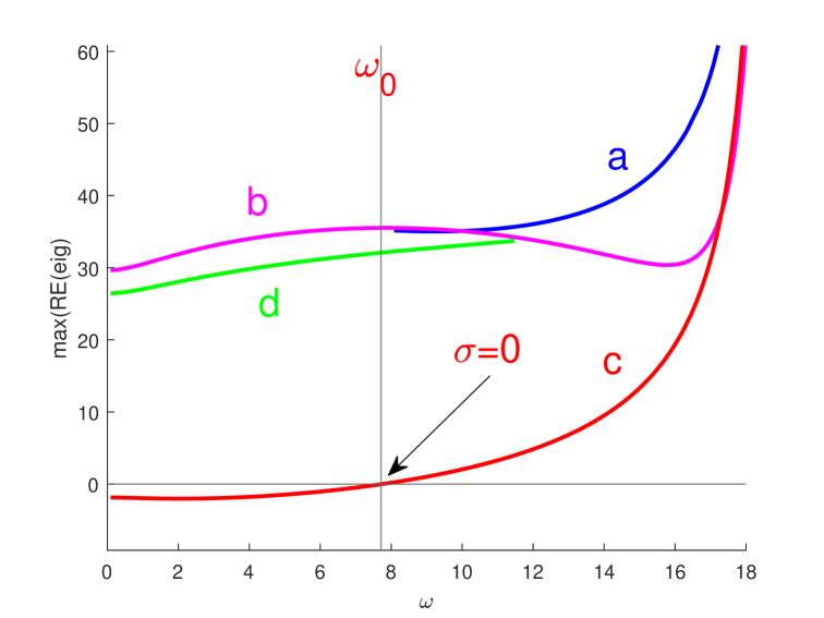
Figure 8: The quantity $max\{Re(\lambda_{i}({\mathbf{{J}}}))\}$ as a function of nondimensional frequency $\omega$, for the four solution branches of planar tumbling.

In summary, we found a full analytical solution for the planar tumbling motion, as well as existence and stability conditions. For known $\delta_{e}$ we obtained an explicit solution for $\omega$. On the other hand, For known $\omega$ we obtain a semi-analytic solution, solving $\delta_{e}$ numerically from a transcendental equation, and then solving the other coordinates analytically.

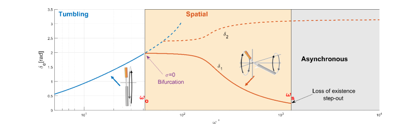
Figure 9: Synchronous solutions branches of the link angle $\delta_{e}$ as a function of nondimensional frequency $\omega$. Blue curve - planar tumbling; red curves - two branches of spatial helical solution. Solid curves - stable solutions; dashed curves - unstable solutions.

IV.4 Spatial helical solution

For the spatial helical solution, we revisit the equilibrium equations (17) and (20). Assuming that $\sin\theta_{e}\neq 0$, they can be simplified to:

$$\omega\sin\delta\left(a_{1}(\delta)\sin(\psi)+b_{1}(\delta)\cos(\psi)\right)=0$$ (38)

$$\sin\beta+\omega b_{2}(\delta)\cos(\psi)+a_{2}(\delta)\sin(\psi)=0$$ (39)

$$\cos\beta\sin\psi+\cos\theta\left(\sin\beta\cos\psi+\omega a_{3}(\delta)\right)=0$$ (40)

$$\alpha\delta=\omega\cos\theta a_{4}(\delta)$$ (41)

where $a_{i}(\delta),b_{i}(\delta)$ are given in (21). From (38) we can find $\psi_{e}$:

$$-\sin\delta\left(a_{1}(\delta)\sin(\psi)+b_{1}(\delta)\cos(\psi)\right)=0$$ (42)

$$\rightarrow\psi_{e}=\arctan\left(-\frac{b_{1}(\delta_{e})}{a_{1}(\delta_{e})}\right)$$ (43)

Substituting $\psi_{e}(\delta_{e})$ into equation (39), one can solve for $\beta_{e}$:

$$\beta_{e}=\arcsin\left(-\omega b_{2}(\delta_{e})\cos(\psi_{e})-a_{2}(\delta_{e})\sin(\psi_{e})\right)$$ (44)

This gives up to two solutions $\beta_{e}$ for each pair of $\delta_{e},\psi_{e}$.
From (41), one can solve for $\theta_{e}$:

$$\theta_{e}=\arccos\left({\frac{\alpha\delta_{e}}{\omega a_{4}(\delta_{e})}}\right)$$ (45)

We obtain a single solution of $\theta_{e}$ in the range $[0,\pi)$ for a given $\delta_{e}$. Substituting the solutions of $\psi,\beta,\theta$ from (43),(44),(45) back into equation (40) gives a scalar equation in $\delta_{e},\omega$:

$$\begin{array}[]{l}\frac{\alpha\delta}{a_{4}}\left(a_{3}-\left(\frac{s_{\psi}b_{1}}{\sqrt{a_{1}^{2}+b_{1}^{2}}}a_{2}-\frac{s_{\psi}a_{1}}{\sqrt{a_{1}^{2}+b_{1}^{2}}}b_{2}\right)\frac{s_{\psi}a_{1}}{\sqrt{a_{1}^{2}+b_{1}^{2}}}\right)\\[12.0pt] =s_{\beta}\sqrt{1-\omega^{2}\left(\frac{s_{\psi}b_{1}}{\sqrt{a_{1}^{2}+b_{1}^{2}}}a_{2}-\frac{s_{\psi}a_{1}}{\sqrt{a_{1}^{2}+b_{1}^{2}}}b_{2}\right)^{2}}\frac{-s_{\psi}b_{1}}{\sqrt{a_{1}^{2}+b_{1}^{2}}}\end{array}$$ (46)

where $a_{i},b_{i}$ are functions of $\delta$ from (21) and $s_{\psi}=\pm 1$ describes the two solutions of $\psi$ from eq. (43), such that $\psi_{-}=\psi_{+}-\pi$, and $s_{\beta}=\mathrm{sign}(\cos\beta_{e})$ describes the two solutions of $\psi$ from eq. (44). Eq. (46) gives a scalar equation which is transcendental in $\delta_{e}$, and can be solved only numerically for given $\omega$. On the other hand, Eq. (46) can be solved analytically for $\omega^{2}$ under given $\delta_{e}$.

Solution multiplicity and symmetries:
Solving equation (43) gives two possible solutions for $\psi_{e}$, represented by $s_{\psi}=\pm 1$. Nevertheless, after choosing a specific solution for $\psi_{e}$, only one solution for $\beta_{e}$ exists in (44). This is because substituting back into (40), it can be shown that $\cos\beta_{e}$ must have a specific sign. For a given frequency $\omega$, equation (46) is transcendental in $\delta$, and may give multiple solutions. It can be shown that these solutions are independent of the choice of $s_{\psi}=\pm 1$ for solution multiplicity of $\psi_{e},\beta_{e}$ in (43) ,(44). Within the range $0<\delta<\pi$ of the joint angle, we show below that there are up to two solutions for (46) under given $\omega$, which are denoted by $\delta_{1},\delta_{2}$. For each of these solutions, there is a single solution of (45) for $\theta_{e}$, and two pairs of solutions of (43) and (44) for $(\beta_{e},\psi_{e})$, depending on the sign $s_{\psi}=\pm 1$. Thus, upon varying $\omega$, we obtain four branches of solutions, denoted by $\{1+\}$, $\{1-\}$, $\{2+\}$ and $\{2-\}$.

Solutions existence: Equations (44),(45) and (46) give three inequalities which determine the range of existence of the solution:

$$\left|-\omega b_{2}(\delta_{e})\cos(\psi_{e})-a_{2}(\delta_{e})\sin(\psi_{e})\right|\leq 1$$ (47)

$$\left|\frac{\alpha\delta_{e}}{\omega a_{4}(\delta_{e})}\right|\leq 1$$ (48)

$$\left(\frac{a_{3}}{a_{4}}\scalebox{0.6}{\mbox{$\displaystyle+$}}\frac{a_{1}(a_{1}b_{2}-a_{2}b_{1})}{a_{4}(a_{1}^{2}+b_{1}^{2})}\right)^{2}\frac{\alpha^{2}\delta^{2}}{b_{1}^{2}}\scalebox{0.6}{\mbox{$\displaystyle-$}}a_{1}^{2}\scalebox{0.6}{\mbox{$\displaystyle-$}}b_{1}^{2}\geq 0$$ (49)

Stability analysis: We now examine stability of the spatial helical solutions using linear analysis, by the Jacobian matrix, calculated analytically.

$$\mathbf{{J}}=\left(\frac{d[\mathbf{{A}}^{-1}\mathbf{{g}}]}{d\mathbf{{q}}}\right)_{\mathbf{{q}}=\mathbf{{q_{e}}}}$$ (50)

In this case, $\mathbf{{J}}$ is a full matrix, rather than block-diagonal as in (36). Figure 9 shows the solution branches of $\delta_{e}$ as function of the nondimensional frequency $\omega$, for both planar tumbling and spatial helical motions. The planar tumbling solution curve is in blue color, and the spatial helical solutions are in red color, two solutions denoted as $\delta_{1}$ (stable branch, solid curve) and $\delta_{2}$ (unstable, dashed). It can be seen that the spatial helical solution starts in the same frequency that the planar tumbling solution loses its stability, at the bifurcation point where $\omega_{0}=\omega_{0}$. Another bifurcation occurs where the planar tumbling branch bifurcates into the unstable branch branch $\delta_{2}$ of spatial helical motion. The stable branch $\delta_{1}$ of spatial helical solution exists in a region from $\omega_{0}$ to $\omega_{s}$. The Step-out frequency $\omega_{s}$ can be found from the existence conditions (47, 48). In frequencies higher than the step-out frequency $\omega_{s}$, we obtain an asynchronous solution, for which the angles $\mathbf{{q}}_{a}(t)$ converge to a steady-state periodic solution, rather than constant values. This solution is similar to the asynchronous solution obtained in [14] for a rigid magnetically-chiral cylinder. Analyzing the linearization eigenvalues of $\mathbf{{J}}$ in (50), it can be shown that upon crossing $\omega=\omega_{s}$, a complex conjugate pair of eigenvalues turns into purely imaginary eigenvalues. This indicates that a Hopf bifurcation point of the synchronous solution occurs at the step-out frequency $\omega=\omega_{s}$ [25].

Swimming speed: We now present expression of the swimming speed $V_{z}$. Applying the simplifying assumptions on the velocity equations (15) gives an expression for the forward speed, in $\mathbf{{\hat{z}}}$ direction:

$$V_{z}=\frac{\omega\sin(2\theta_{e})(\cos(\delta_{e})+1)(\cos(\delta_{e}+\psi_{e})-\cos(\psi_{e}))}{8c_{n1}l_{1}(3-\cos(\delta_{e}))}$$ (51)

One can also examine the pitch, the displacement per cycle, defined as $\Delta z=V_{z}\frac{2\pi}{\omega}$.
The planar tumbling solution with $\sin\theta_{e}=0$, gives zero propulsion $V_{z}=0$. By substituting the spatial helical solution into (51), one obtains an expression for $V_{z}$ that only depends on the joint angle $\delta_{e}$, which, in turn, depends on the nondimensional frequency $\omega$. Note that solution multiplicity $s_{\psi}=\pm 1$ for $\psi_{e}$ simply results in reversing the sign of $V_{z}$, so that solutions $\{i-\}$ are identical to solutions $\{i+\}$, except for swimming in $-\mathbf{{\hat{z}}}$ direction rather than $+\mathbf{{\hat{z}}}$. Figures 10,11, show the speed $V_{z}$ and pitch $\Delta z$ as a function of $\omega$, for both stable (solid) and unstable (dashed) branches of spatial helical motion (for $\omega<\omega_{0}$, the only solution is planar tumbling so that $V_{z}=0$). It can be seen that for the stable branch, one obtains maximal values of $V_{z}$ and $\Delta z$ for two different optimal frequencies, denoted by $\omega_{v},\omega_{z}$. In higher frequencies, above the step-out frequency $\omega_{s}$, the spatial helical solution ceases to exists and an asynchronous solution begins. The asynchronous solution’s mean speed and pitch continue the line smoothly from the synchronous spatial helical solution [25]. Furthermore, in [25] we also developed an approximate formulation of the helical motion using perturbation expansion at the limit of low stiffness, allowing us to obtain explicit approximate expressions for optimal frequency and swimming speed.

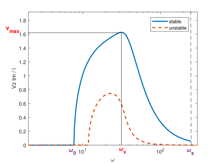
Figure 10: Normalized Speed $\frac{t_{m}}{l}V_{z}$ of the synchronous solution as a function of nondimensional frequency $\omega$.

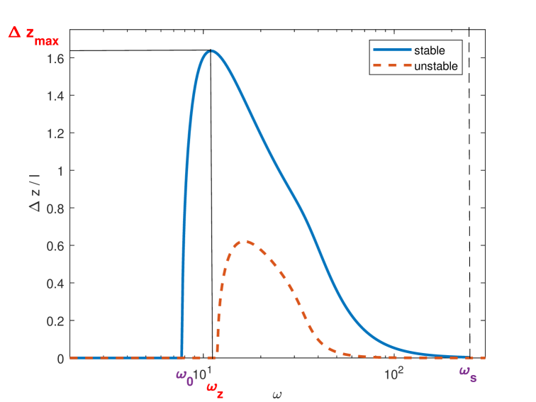
Figure 11: Normalized pitch $\Delta z/l$ of the synchronous solution as a function of nondimensional frequency $\omega$.

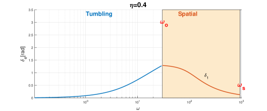
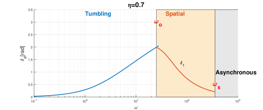
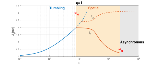
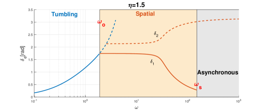
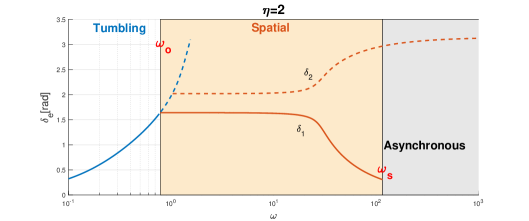
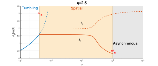
Figure 12: Synchronous solutions of the joint angle $\delta$ as a function of the nondimensional frequency $\omega$, for different values of length ratio $\eta$. Blue curve - planar tumbling; red curves - branches of spatial helical solution. Solid curves - stable solutions; dashed curves - unstable solutions.

V Analysis of generalized case

In this section, we study a general case where some of the simplifying assumptions from previous section are relaxed. First, we analyze the cases of unequal link’s length and of a conically rotating magnetic field. Next, we show some numerical optimizations for those and other cases.

V.1 Unequal links’ length

We now study the effect of unequal links’ lengths. We define a new variable for the ratio of the lengths $\eta=l_{2}/l_{1}$. We revisit the equilibrium equations (19) applying the assumptions from section IV.2 above, while assuming $l_{2}=\eta l_{1}$. Note that this also implies scaling on the drag coefficients, as:

$$h=0;c_{t_{i}}=\frac{1}{2}c_{n_{i}};d_{n_{i}}=\frac{1}{12}c_{n_{i}}l_{i}^{2};d_{t_{i}}=0;c_{n_{2}}=\eta c_{n_{1}}$$ (52)

From (52), we obtain the generalized equilibrium equations. Those equations are the same as in (17). However, the expressions for $a_{i}(\delta_{e}),b_{i}(\delta_{e})$ are different from (21), and are given in Table 2 below.

Table 2:

$a_{1}(\delta)=-\frac{\eta\sin\delta_{e}(\eta+4)}{12(\eta+1)}$

$b_{1}(\delta)=\frac{\sin\delta_{e}(6+\eta\cos\delta_{e}(7+\eta))}{24(\eta+1)}$

$a_{2}(\delta)=\frac{\eta^{2}\sin\delta_{e}(3+\eta\cos\delta_{e}(4+\eta))}{12(\eta+1)}$

$b_{2}(\delta)=-\frac{\eta^{3}\cos^{2}\delta_{e}(4+\eta)+6\eta^{2}\cos\delta_{e}+1+4\eta}{12(\eta+1)}$

$a_{3}(\delta)=-\frac{(\eta+1)\left(2+6\eta+2\eta^{2}+6\eta^{3}+2\eta^{4}+12\eta^{2}\cos\delta_{e}(2-2\eta+2\eta^{2})\right)}{20\eta+8\eta^{2}-4\eta\cos^{2}\delta_{e}+8}$

$a_{4}(\delta)=-\frac{\eta^{2}\left(8\eta+\eta^{3}+8\eta^{2}+cos\delta_{e}(6+6\eta+2\eta\cos\delta_{e})\right)}{4\left(5\eta+2\eta^{2}-\eta\cos^{2}\delta_{e}+2\right)}$

In fact, the expressions in Table 2 are generalization of (21) to the case of $\eta\neq 1$.
We are able to solve the equilibrium equations (17) using the same steps taken above. Nevertheless, the multiplicity of solution branches and their existence conditions now depend also on the ratio $\eta$.
In Figure 12, we present the branches of tumbling and helical solutions of the joint angle $\delta=\delta_{e}$ as a function of the nondimensional frequency $\omega$, for different values of length ratio $\eta$. Solid lines denote stable solutions while dashed lines denote unstable ones. From the plots, we can see that in low values of $\eta<1$, i.e. shorter tail link, the planar tumbling solution exists in a wider range of nondimensional frequencies, whereas the spatial helical solution emerges at a larger $\omega$. In addition, for low $\eta$ only the stable solution branches exist, and the joint angle $\delta_{e}$ attains smaller values. In larger values of $\eta$, unstable solution branches emerge and both $\omega_{0}$ and $\omega_{s}$ are decreasing with growing $\eta$. We can also notice that the maximal joint angle $\delta_{e}$ is increasing with $\eta$ up to $\eta\approx 0.8,\delta_{e}\approx 2$. After this point, $\delta_{e}$ decreases until reaching $\delta_{e}\to\pi/2$ for the stable solution.
Next, we examine the influence of $\eta$ on swimming speed. The expression for $V_{z}$ remains the same as in (51), except that the equilibrium angles $\delta_{e},\theta_{e},\psi_{e}$ change with $\eta$. In Figures 13 and 14, we plot the normalized pitch $\Delta z/l_{1}$ and speed $\frac{t_{m}}{l_{1}}V_{z}$ as a function of the links’ length ratio $\eta$ for given fixed frequencies. We obtain maximal pitch or speed, which are attained at different values of $\eta$ depending on frequency $\omega$. The plots indicate that a combined optimum exists in both the frequency $\omega$ and in the length ratio $\eta$, which is further examined below in Figures 19 and 20.

V.2 Conically rotating magnetic field

We now consider the case of equal links’ lengths $\eta=1$, while assuming a magnetic field with $h\neq 0$: The equilibrium equations (17) are generalized as:

$$\omega\sin\theta_{e}\sin\delta_{e}\left(a_{1}(\delta_{e})\sin(\psi_{e})+b_{1}(\delta_{e})\cos(\psi_{e})\right)=0$$

$$\sin\theta_{e}\left(\sin\beta_{e}+\omega b_{2}(\delta_{e})\cos(\psi_{e})+a_{2}(\delta_{e})\sin(\psi_{e})\right)$$

$${\color[rgb]{0,0,1}+h\cos\theta_{e}}=0$$

$$\cos\beta_{e}\sin\psi_{e}+\cos\theta_{e}\left(\sin\beta_{e}\cos\psi_{e}+\omega a_{3}(\delta_{e})\right)$$

$${\color[rgb]{0,0,1}-h\cos\psi_{e}\sin\theta_{e}}=0$$

$$\alpha\delta_{e}=\omega\cos\theta_{e}a_{4}(\delta_{e})$$ (53)

While $a_{i}(\delta_{e}),b_{i}(\delta_{e})$ remain the same as in (21). The equilibrium equations (53) are different from the previous cases, and the added effect of the constant component $h$ is marked in blue. That is, when setting $h=0$, equations (53) reduce back to (38)-(41). Equations (53) are solved in a similar way as in the case of $h=0$ above. Importantly, it can be shown that $\sin\theta_{e}=0$ is no longer a solution of (53), in contrast to the previous case with $h=0$. This implies that the planar tumbling solution no longer exists for $h\neq 0$. The solution of first equation of (53) for spatial helical motion remains:

$$\psi_{e}=\arctan\left(-\frac{b_{1}(\delta_{e})}{a_{1}(\delta_{e})}\right)$$ (54)

The solution of the $4^{th}$ equation of (53) also remains:

$$\theta_{e}=\arccos\left(\frac{\alpha\delta_{e}}{\omega a_{4}(\delta_{e})}\right)$$ (55)

From the second equation in (53) we obtain the new solution for $\beta_{e}$:

$$\beta_{e}=\arcsin\left(\text{-}\omega(b_{2}(\delta_{e})\cos(\psi_{e})\text{+}a_{2}(\delta_{e})\sin(\psi_{e})){\color[rgb]{0,0,1}-\frac{h\cos\theta_{e}}{\sin\theta_{e}}}\right)$$ (56)

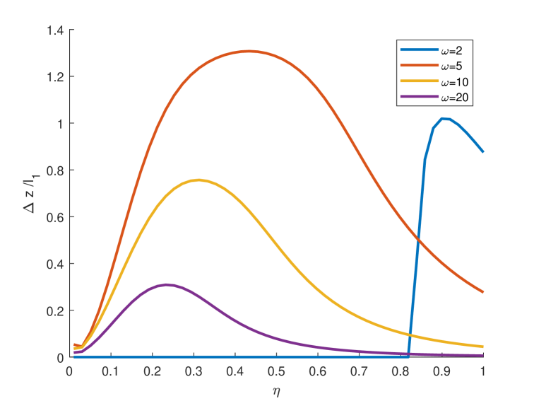
Figure 13: Normalized pitch $\Delta z/l_{1}$ in the stable solution branch, plotted as function of links’ length ratio $\eta$ for different values of nondimensional frequency $\omega$.

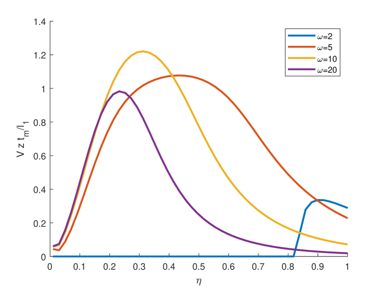
Figure 14: Normalized Speed $\frac{t_{m}}{l_{1}}V_{z}$ in the stable solution branch, plotted as function of links’ length ratio $\eta$ for different values of nondimensional frequency $\omega$.

Finally, by substituting the solutions (54), (55) and (56) into the third equation of (53), we obtain a scalar equation in $\delta,\omega$. This equation is transcendental in $\delta_{e}$ and high-degree polynomial in $\omega$, which can be solved numerically for known $\delta_{e}$ or $\omega$. For given nondimensional frequency $\omega$, we numerically obtain up to two solutions for $\delta_{e}$ within the range $(0,\pi)$. Importantly, the addition of $h\neq 0$ violates previous symmetries of solutions with respect to the choice of $s_{\psi}=\pm 1$ for multiplicity of the solutions for $\psi_{e}$ and $\beta_{e}$. That is, we obtain four different solution branches $\{1+\}$, $\{1-\}$, $\{2+\}$ and $\{2-\}$, which do not satisfy symmetry interrelations as in the case of $h=0$. Stability of the solution branches can be determined by calculating eigenvalues of the Jacobian matrix, as defined in (50).

Figure 15 plots the four different solution branches of the joint angle $\delta_{e}$ as a function of the nondimensional frequency $\omega$, under a conically-rotating magnetic field with constant component $h=0.2$. Stable solutions are marked as blue curves while unstable solutions are marked as red curves. It can be seen that solution branch $\{1+\}$ is stable and solution branch $\{2+\}$ is unstable for the entire range of nondimensional frequencies $\omega$, similarly to the previous case of $h=0$. However, branches $\{1-\}$ and $\{2-\}$ include stability transitions upon varying $\omega$. This interesting phenomenon is similar to stability transitions of the same micro-swimmer model under a planar oscillating magnetic field, which were studied in [20]. Figure 16 plots the normalized swimming speed $\frac{t_{m}}{l}V_{z}$ as a function of the nondimensional frequency for all solution branches, under the same case of $h=0.2$. It can be seen that the solution branches $\{i+\}$ have $V_{z}>0$ and branches $\{i-\}$ have $V_{z}<0$. Each branch has an optimal frequency for which $|V_{z}|$ is maximized, but symmetry between $\pm$ branches is lost.

Figure 17 plots all solution branches of the joint angle $\delta_{e}$ as a function of the nondimensional frequency $\omega$ for a larger constant component, $h=1$. The normalized swimming speed $\frac{t_{m}}{l}V_{z}$ as a function of the nondimensional frequency in all solution branches for $h=1$ is plotted in Figure 18. Stable solutions are marked as blue curves while unstable solutions are marked as red curves. It can be seen that the solution branch $\{2-\}$ no longer exists for this case, and that the maximal swimming speed for this case is larger than that of $h=0.2$. This motivates combined optimization of swimming speed upon varying both frequnecy and $h$, as discussed below.

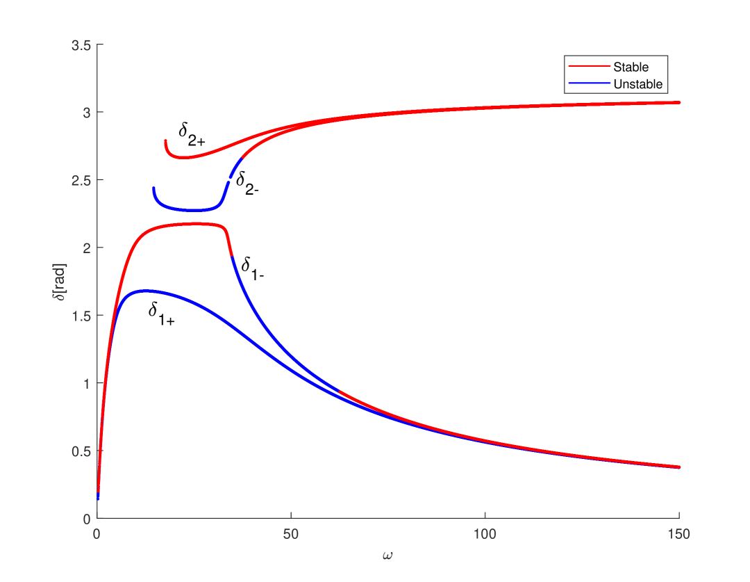
Figure 15: Solution branches for the joint angle $\delta_{e}$ as a function of nondimensional frequency $\omega$, under a conically-rotating magnetic field with constant component $h=0.2$. Blue curves - stable solution. Red curves - unstable solution.

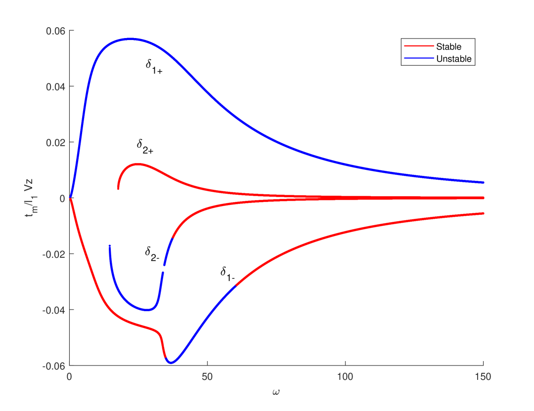
Figure 16: Normalized swimming speed $\frac{t_{m}}{l}V_{z}$ for all solution branches as a function of nondimensional frequency $\omega$, under a conically-rotating magnetic field with constant component $h=0.2$. Blue curves - stable solution. Red curves - unstable solution.

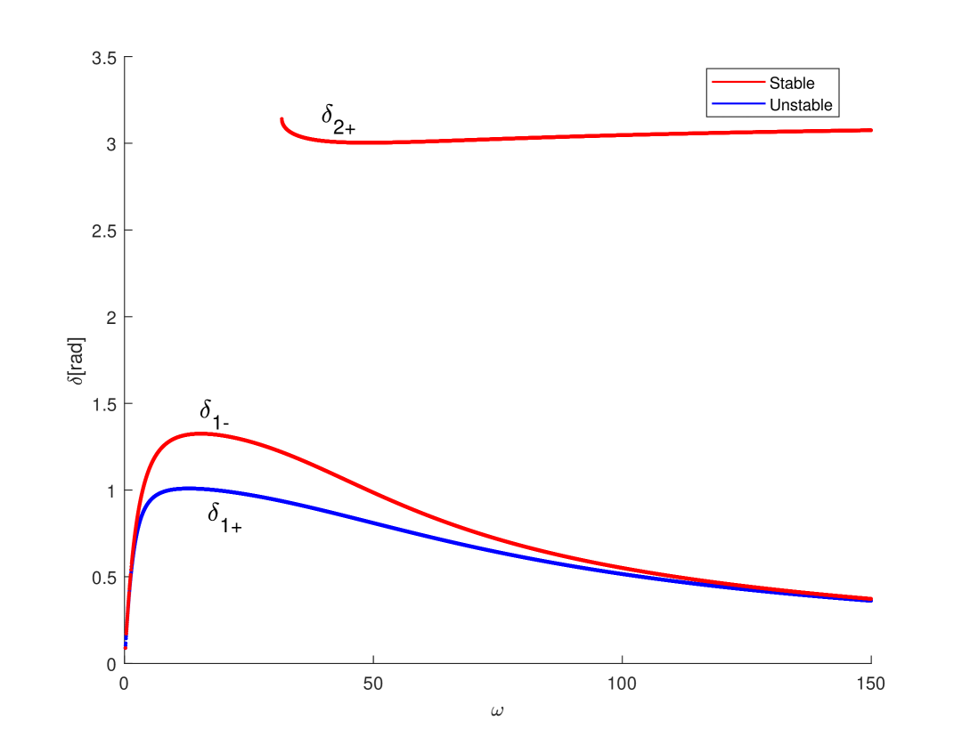
Figure 17: Solution branches for the joint angle $\delta_{e}$ as a function of nondimensional frequency $\omega$, under a conically-rotating magnetic field with constant component $h=1$. Blue curves - stable solution. Red curves - unstable solution.

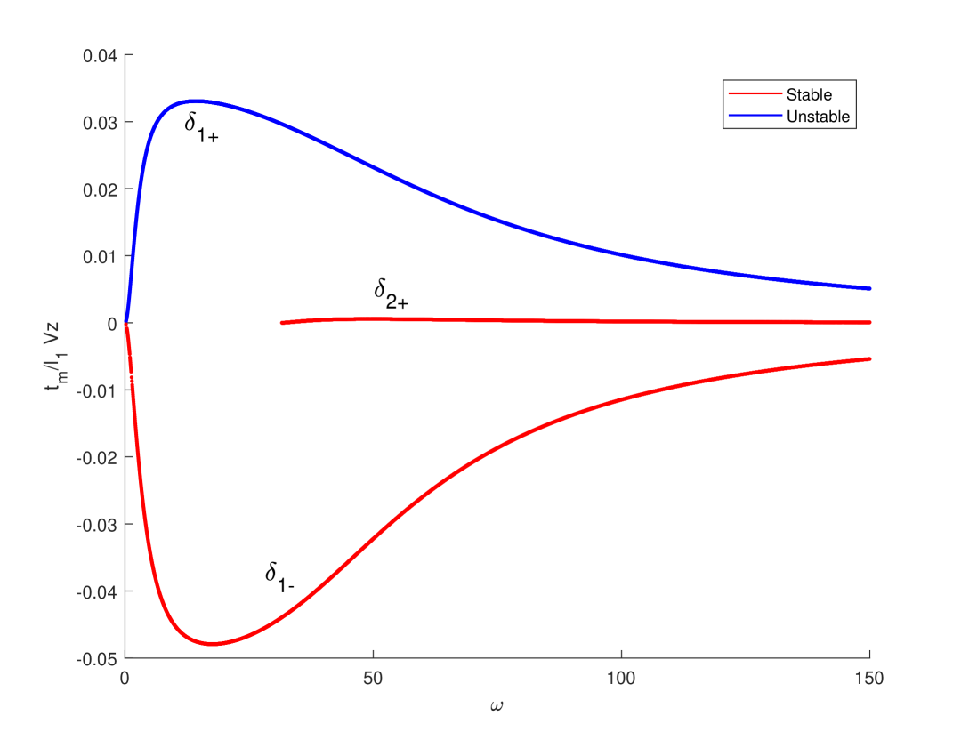
Figure 18: Normalized swimming speed $\frac{t_{m}}{l}V_{z}$ for all solution branches as a function of nondimensional frequency $\omega$, under a conically-rotating magnetic field with constant component $h=1$. Blue curves - stable solution. Red curves - unstable solution.

V.3 Numerical parametric optimizations

We now demonstrate optimization of the nano-swimmer’s performance with respect to various parameters, combined with actuation frequency. In each case, we set nominal values of physical parameters as given in (11), except for one chosen parameter which is varied, along with the actuation frequency $\Omega$. We obtain the swimmer’s steady-state solution of spatial helical motion, calculate the mean speed $V_{z}$ and pitch $\Delta z$ and show both of them in contour plots. We consider only solution branch $\{1+\}$, which is stable for all $\Omega$. (In cases where $h=0$, the solution branch $\{1-\}$ is a mirror reflection of $\{1+\}$, with same speed $|V_{z}|$ in negative direction).

First, we vary the links’ length ratio $\eta$ while the head link’s length $l_{1}$ is held constant. Figures 19 and 20 show contour maps for the pitch $\Delta z$ and speed $V_{z}$ as a function of the frequency $\Omega$ and links’ length ratio $\eta$.

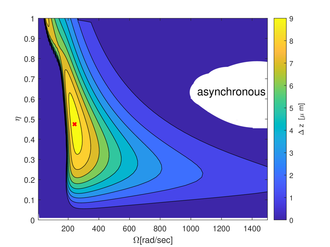
Figure 19: Contour map of the pitch $\Delta z$ as function of the frequency $\Omega$ and links’ length ratio $\eta$

In Figure 19, there is one optimum point for the pitch $\Delta z$, at $\eta=0.45,\Omega=240[rad/sec]$.

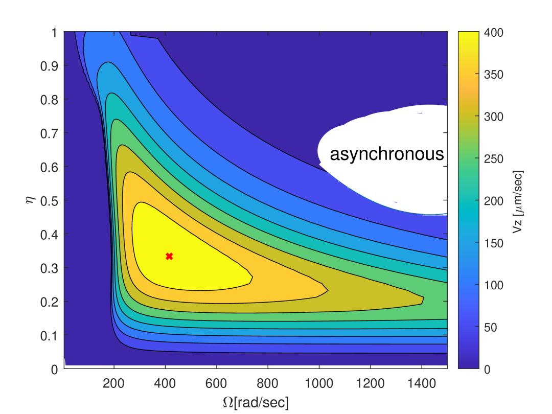
Figure 20: Contour map of the speed $V_{z}$ as function of the frequency $\Omega$ and links’ length ratio $\eta$

In Figure 20, there is one optimum point for the speed $V_{z}$, at $\eta=0.33,\Omega=450[rad/sec]$. The white region in both figures represents the asynchronous regime beyond step-out frequency.

Next, we examine the case of conically-rotating magnetic field, with varying constant component $h$. Contour plots of the pitch $\Delta z$ and speed $V_{z}$ as a function of frequency $\Omega$ and $h$ are shown in Figures 21 and 22.

Figure 21: Contour map of the pitch $\Delta z$ as function of the frequency $\Omega$ and conic field component $\mathbf{{B}}(t)=b(\sin(\Omega t)\hat{\mathbf{{x}}}+\cos(\Omega t)\hat{\mathbf{{y}}}+h\hat{\mathbf{{z}}})$

In Figure 21, there is one optimum for the pitch $\Delta z$, at $h=0.57,\Omega=24[rad/sec]$.

Figure 22: Contour map of the pitch $V_{z}$ as function of the frequency $\Omega$ and conic field component $\mathbf{{B}}(t)=b(\sin(\Omega t)\hat{\mathbf{{x}}}+\cos(\Omega t)\hat{\mathbf{{y}}}+h\hat{\mathbf{{z}}})$

In Figure 22, there is one optimum for the speed $V_{z}$, at $h=0,\Omega=160[rad/sec]$. Note that the maximal forward speed is obtained for the case $h=0$.

Next, we examine optimization with respect to the joint’s torsional stiffness $k$. Contour plots of $\Delta z$ and $V_{z}$ as a function of $\Omega$ and $k$ are shown in Figures 23 and 24.

Figure 23: Contour map of the pitch $\Delta z$ as function of the frequency $\Omega$ and joint’s stiffness component $k$

In Figure 23, there is one optimum for the pitch $\Delta z$, at $k=1.3\cdot 10^{-16}[N\cdot m],\Omega=65[rad/sec]$.

Figure 24: Contour map of the pitch $V_{z}$ as function of the frequency $\Omega$ and joint’s stiffness component $k$

In Figure 24, there is one optimum for the speed $V_{z}$, at $k=1.3\cdot 10^{-16}[N\cdot m],\Omega=119[rad/sec]$.

Finally, we examine optimization with respect to the magnetic field’s magnitude $b$. Contour plots of $\Delta z$ and $V_{z}$ as a function of $\Omega$ and $b$ are shown in Figures 25 and 26.

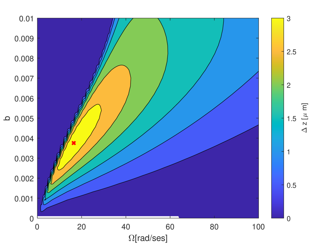
Figure 25: Contour map of the pitch $\Delta z$ as function of the frequency $\Omega$ and magnetic field’s amplitude component $b$

In Figure 25, there is one optimum pitch, at $b=3.7[mT],\Omega=16[rad/sec]$.

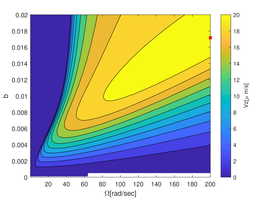
Figure 26: Contour map of the pitch $V_{z}$ as function of the frequency $\Omega$ and magnetic field’s amplitude component $b$

In Figure 26, there is an optimum for $V_{z}$ at the limit of the plot, at $b=17[mT],\Omega=200[rad/sec]$. Some more numerical optimization results with respect to other physical parameters can be found in [25].

VI Concluding discussion

In this work, we revisited the simplified two-link model of a nano-swimmer with flexible hinge under a rotating magnetic field, which was studied numerically and demonstrated experimentally in [21]. We explicitly formulated and analyzed the nano-swimmer’s nonlinear dynamic equations of spatial motion. We reduced the dynamic equations to a 4-DOF time-invariant system using transformation of variables. We obtained explicit analytic solutions for synchronous motion under simplifying assumptions, for both regimes of in-plane tumbling and spatial helical corkscrew swimming. We conducted stability analysis of the solution branches, and found stability transitions and bifurcations of multiple solution branches. We obtained an explicit expression for the forward speed and pitch, and found optimal frequencies maximizing speed and pitch. Finally, we presented analysis of the influence of additional effects such as unequal links length and conically-rotating magnetic field, as well as numerical parametric optimization.

We now briefly discuss the limitations of our current analysis. First, the suggested swimmer model is simple and does not represent the fabricated swimmer accurately. It assumed a pointed uni-axial hinge, while the actual hinge is a flexible beam that undergoes both bending and torsion. In addition, our model did not account for hydrodynamic interaction between the links, and did not consider the influence of boundaries of the fluid domains. All those effects can be implemented into a new swimmer model in possible future extension of the research. Other possible generalizations can be interesting for future research, such as the effect of varying the directionality of link’s magnetization, nano-swimmer composed of multiple magnetic links, flexible links, and additional choices in the time-varying profile of the external magnetic field.

Despite all limitations, this work showed a simple model that captures most of dominating phenomena observed in experiments on the fabricated nano-swimmer, allowing us to better understand the dynamics of magnetic nano-swimmers. With this improved understanding, new and optimized magnetic nano-swimmers may be fabricated, which eventually will allow the designing of artificial magnetic nano-bots for bio-medical purposes advancing towards the grand challenge of micro-nano-biomedical robotics.

Acknowledgment: This work has been supported by Israel Science Foundation, under grant no. 1382/23.

References

- Li et al. [2017] J. Li, B. E.-F. de Ávila, W. Gao, L. Zhang, and J. Wang, Micro/nanorobots for biomedicine: Delivery, surgery, sensing, and detoxification, Science Robotics (2017).
- Crenshaw [1996] H. C. Crenshaw, A new look at locomotion in microorganisms: rotating and translating, American Zoologist 36, 608 (1996).
- Purcell [1977] E. M. Purcell, Life at low Reynolds number, American J. P 45, 3 (1977).
- Balk et al. [2014] A. L. Balk, L. O. Mair, P. P. Mathai, P. N. Patrone, W. Wang, S. Ahmed, T. E. Mallouk, J. A. Liddle, and S. M. Stavis, Kilohertz rotation of nanorods propelled by ultrasound, traced by microvortex advection of nanoparticles, ACS Nano 8, 8300 (2014).
- Chen et al. [2018] X.-Z. Chen, B. Jang, D. Ahmed, C. Hu, C. De Marco, M. Hoop, F. Mushtaq, B. J. Nelson, and S. Pané, Small-scale machines driven by external power sources, Advanced Materials 30, 1705061 (2018).
- Xu et al. [2017] T. Xu, W. Gao, L.-P. Xu, X. Zhang, and S. Wang, Fuel-free synthetic micro-/nanomachines, Advanced Materials 29, 1603250 (2017).
- Dreyfus et al. [2005] R. Dreyfus, J. Baudry, M. L. Roper, M. Fermigier, H. A. Stone, and J. Bibette, Microscopic artificial swimmers, Nature 437, 862 (2005).
- Zhang et al. [2009a] L. Zhang, J. J. Abbott, L. Dong, B. E. Kratochvil, D. Bell, and B. J. Nelson, Artificial bacterial flagella: Fabrication and magnetic control, Applied Physics Letters 94, 064107 (2009a).
- Wang and Pumera [2015] H. Wang and M. Pumera, Fabrication of micro/nanoscale motors, Chemical Reviews 115, 8704 (2015).
- Gao et al. [2010] W. Gao, S. Sattayasamitsathit, K. M. Manesh, D. Weihs, and J. Wang, Magnetically powered flexible metal nanowire motors, Journal of the American Chemical Society 132, 14403 (2010).
- Jang et al. [2018] B. Jang, A. Aho, B. J. Nelson, and S. Pané, Fabrication and locomotion of flexible nanoswimmers, in 2018 IEEE/RSJ International Conference on Intelligent Robots and Systems (IROS) (IEEE, 2018) pp. 6193–6198.
- Ishiyama et al. [2001] K. Ishiyama, M. Sendoh, A. Yamazaki, and K. Arai, Swimming micro-machine driven by magnetic torque, Sensors and Actuators A: Physical 91, 141 (2001).
- Ghosh et al. [2013] A. Ghosh, P. Mandal, S. Karmakar, and A. Ghosh, Analytical theory and stability analysis of an elongated nanoscale object under external torque, Physical Chemistry Chemical Physics 15, 10817 (2013).
- Morozov and Leshansky [2014] K. I. Morozov and A. M. Leshansky, The chiral magnetic nanomotors, Nanoscale 6, 1580 (2014).
- Gao et al. [2012] W. Gao, D. Kagan, O. S. Pak, C. Clawson, S. Campuzano, E. Chuluun-Erdene, E. Shipton, E. E. Fullerton, L. Zhang, E. Lauga, et al., Cargo-towing fuel-free magnetic nanoswimmers for targeted drug delivery, small 8, 460 (2012).
- Pak et al. [2011] O. S. Pak, W. Gao, J. Wang, and E. Lauga, High-speed propulsion of flexible nanowire motors: Theory and experiments, Soft Matter 7, 8169 (2011).
- Mirzae et al. [2020] Y. Mirzae, B. Y. Rubinstein, K. I. Morozov, and A. M. Leshansky, Modeling propulsion of soft magnetic nanowires, Frontiers in Robotics and AI 7, 595777 (2020).
- Gutman and Or [2014] E. Gutman and Y. Or, Simple model of a planar undulating magnetic microswimmer, Physical Review E 90, 013012 (2014).
- Harduf et al. [2018] Y. Harduf, D. Jin, Y. Or, and L. Zhang, Nonlinear parametric excitation effect induces stability transitions in swimming direction of flexible superparamagnetic microswimmers, Soft Robotics 5, 389 (2018).
- Paul et al. [2023] J. Paul, Y. Or, and O. V. Gendelman, Nonlinear dynamics and bifurcations of a planar undulating magnetic microswimmer, Physical Review E 107, 054211 (2023).
- Wu et al. [2021] J. Wu, B. Jang, Y. Harduf, Z. Chapnik, Ö. B. Avci, X. Chen, J. Puigmartí-Luis, O. Ergeneman, B. J. Nelson, Y. Or, et al., Helical klinotactic locomotion of two-link nanoswimmers with dual-function drug-loaded soft polysaccharide hinges, Advanced Science 8, 2004458 (2021).
- Happel and Brenner [2012] J. Happel and H. Brenner, Low Reynolds number hydrodynamics: with special applications to particulate media, Vol. 1 (Springer Science & Business Media, 2012).
- Jeffery [1922] G. B. Jeffery, The motion of ellipsoidal particles immersed in a viscous fluid, Proceedings of the Royal Society of London. Series A, Containing papers of a mathematical and physical character 102, 161 (1922).
- Ortega and Garcıa de la Torre [2003] A. Ortega and J. Garcıa de la Torre, Hydrodynamic properties of rodlike and disklike particles in dilute solution, The Journal of C. P 119, 9914 (2003).
- Chapnik [2022] Z. Chapnik, Spatial dynamics of flexible nano-swimmers under a rotating magnetic field, https://yizhar.net.technion.ac.il/supervised-students-theses/, Msc Thesis (2022).
- Zhang et al. [2009b] L. Zhang, J. J. Abbott, L. Dong, K. E. Peyer, B. E. Kratochvil, H. Zhang, C. Bergeles, and B. J. Nelson, Characterizing the swimming properties of artificial bacterial flagella, Nano letters 9, 3663 (2009b).