Quenched Entanglement Harvesting

Abstract

Ultracold fermionic atoms in an optical lattice, with a sudden position-dependent change (a quench) in the effective dispersion relation, have been proposed by Rodríguez-Laguna et al. as an analogue spacetime test of the Unruh effect. We provide new support for this analogue by analysing the entanglement of a scalar field in a $(1+1)$-dimensional continuum spacetime with a similar quench, and the harvesting of this entanglement by a pair of Unruh-DeWitt detectors. We present numerical evidence that the concurrence and mutual information harvested by the detectors are qualitatively similar to those in Rindler spacetime, but they exhibit a small yet noticeable variation when the energy pulse created by the quench crosses the detectors. These findings provide further motivation to implement the experimental proposal of Rodríguez-Laguna et al.

I Introduction

It has long been known that the vacuum state of a quantum field contains entanglement [1, 2]. This has led to the expectation that such entanglement can be extracted, or harvested, by physical devices or objects such as atoms [3, 4, 5], and that this can take place even when these objects are spacelike separated.

The general paradigm for the entanglement harvesting protocol [6] considers two initially uncorrelated detectors that locally interact with a quantum field in some state (typically the vacuum state). The amount of harvested correlations is sensitive to both the composition and states of the detectors (for example, their motion) [7, 8, 9, 10, 11, 12, 13, 14, 15] as well as the spacetime background [16, 17, 18, 19, 20, 21, 22, 23, 24, 25, 26, 27, 28, 29, 30, 31].

This effect is extraordinarily difficult to measure in vacuum, particularly given the length and time scales involved. This has motivated efforts to consider alternative settings in which entanglement harvesting can be observed, with recent experiments detecting correlations of the electromagnetic ground state in a ZnTe crystal [32, 33, 34] providing further impetus to this end. Indeed there has been a recent proposal to extract entanglement from the ZnTe crystal [35], as well as from quantum surface fluctuations of a Bose-Einstein condensate [36].

New analogue settings that behave as relativistic quantum field theories, originally proposed in the context of testing the Unruh Effect, provide a promising avenue in which to test entanglement harvesting. These have a causal structure that is bounded by the speed of sound of the medium and not the speed of light, allowing for entanglement harvesting properties to be within reach of measurement techniques.

Amongst the various analog settings, one of particular note is that proposed by Rodríguez-Laguna et al [37] and Kosior et al [38], in which an optical lattice with ultracold fermionic atoms is used to model a Dirac field in a curved spacetime in a setup that permits control of the low energy effective Hamiltonian of the system. To model the Unruh effect, the Hamiltonian is first set to be that of a free Dirac fermion in Minkowski spacetime. Then there is a “quench” of the Hamiltonian, so that it effectively becomes the one associated with a free fermion in a spacetime whose $(1+1)$-dimensional part is

$$ds^{2}=-\chi^{2}d\eta^{2}+d\chi^{2},$$ (1)

known as the Rindler metric.

In this proposal, the field is initialized in its Minkowski vacuum state, after which it evolves through the quench [37]. Numerical simulations indicated that Unruh-like effects should be present, despite the analog nature of the proposed experiment. It was subsequently argued in a different way that Unruh like effects should be present in these lattice setups [39]. Specifically, it was shown that a free massless scalar field in the $(1+1)$-dimensional quench spacetime (described in detail below in Section II) experiences an Unruh effect in the post-quench region. This provides further evidence that Unruh-like effects should be observable in ultracold-fermionic-atom lattices.

Here we study the entanglement properties of a massless scalar in this $(1+1)$-dimensional quench spacetime. In particular, we investigate the entanglement harvesting properties of a pair of accelerated Unruh-DeWitt (UDW) detectors [40, 41] in this setup. We find that indeed the harvesting phenomenon is present, and exhibits similar properties to the entanglement harvested by UDW detectors on accelerated trajectories in flat Minkowski spacetime. Additionally, we show that the entanglement harvested exhibits a small but distinct dependence on the energy pulse that the quench creates in the post-quench part of the spacetime.

Our results strengthen the expectation that entanglement harvesting should also be present in analog setups [37], [38], providing further motivation to realize their experimental proposals.

The structure of our paper is as follows. In Section II we provide a brief description of the quench spacetime and the stress energy tensor of a quantised massless scalar field therein. In Section III we describe the Wightman function, trajectories, and switching functions used to calculate the entanglement harvested. In Section IV, we describe in detail the specific parameter ranges over which the entanglement was calculated. In Section V we show the obtained entanglement harvesting results, making some brief remarks about them, and finally in Section VI we report our conclusions of the work. In Appendix A, we briefly discuss the code used for the numerical entanglement calculations and outline the validation checks taken to ensure the robustness of the results.

II The Quench spacetime

The quench spacetime [39] consists of a flat spacetime in the past of a distinguished spacelike hypersurface, and of a regularized double Rindler spacetime in the future of this hypersurface. The metric reads

$$ds^{2}=\begin{cases}-(\chi^{2}+b^{2})d\eta^{2}+d\chi^{2}&\text{for }\eta\geq 0\\ -dt^{2}+dx^{2}&\text{for }t<0\end{cases}$$ (2)

using Rindler-like coordinates in the future half, where $b$ is a positive parameter, and Minkowski coordinates in the past half. The quench occurs at $t=0=\eta$, where the halves are joined so that $x=\chi$. In the future half, the metric may be expressed in the conformally flat form

$$ds^{2}=b^{2}\cosh^{2}(y)(-d\eta^{2}+dy^{2})$$ (3)

through the coordinate transformation

$$\chi=b\sinh(y).$$ (4)

This spacetime has several features that make it a good candidate for modelling the setup proposed in [37]. Apart from the obvious point that it models rapid transition between flat Minkowski and a Rindler like spacetime (which is the desired situation for experiment [37, 38]), it possesses two additional properties that make it resemble the proposed setup:

• In the optical lattice case, it is expected that the $\chi=0$ singularity in (1) gets removed by the discrete nature of the lattice. In the quench spacetime (2), the singularity has been regularized by the deformation introduced by the $b$ parameter.

• In the optical lattice, it is expected that there are no Rindler wedges bordered by Killing horizons and separated by future/past causal diamonds. In the quench spacetime it is also the case that those features are not present, since the spacetime is geodesically complete, under a reasonable interpretation of a ‘geodesic’ across the metric discontinuity at $\eta=0=t$.

For a quantum massless scalar field on the quench spacetime, prepared in the Minkowski vacuum in the pre-quench region, the Wightman function in the post-quench region may be expressed in terms of elementary functions [39]. This makes it possible to compute in the post-quench region quantum observables in terms of elementary functions. We recall here that the stress-energy tensor (SET) reads [39]

$$T_{\eta\eta}=\frac{1}{8\pi\cosh^{2}\!y}-\frac{1}{16\pi}\left(\frac{1}{\cosh^{2}(\eta-y)}+\frac{1}{\cosh^{2}(\eta+y)}\right)$$ (5)

$$T_{yy}=\frac{1}{24\pi\cosh^{2}\!y}-\frac{1}{16\pi}\left(\frac{1}{\cosh^{2}(\eta-y)}+\frac{1}{\cosh^{2}(\eta+y)}\right)$$ (6)

$$T_{\eta y}=\frac{1}{16\pi}\left(\frac{1}{\cosh^{2}(\eta-y)}-\frac{1}{\cosh^{2}(\eta+y)}\right)$$ (7)

These expressions show that the SET has pulses travelling along the light cones $y=\pm\eta$, with a characteristic width of order unity in $y$ at a given $\eta$, and a characteristic duration of order unity in $\eta$ at each $y$ with $|y|\gtrsim 1$. In what follows we will consider how these pulses are correlated with the entanglement harvested by a pair of model particle detectors.

III Ingredients for Entanglement Harvesting

III.1 Preliminaries

We shall model a UDW detector [40, 41] as a pointlike qubit having two energy levels, denoted by $|g\rangle$ and $|e\rangle$, with the respective energy eigenvalues $0$ and $\Omega$. For $\Omega>0$, $|g\rangle$ is the ground state and $|e\rangle$ is the excited state; for $\Omega<0$, the roles of $|g\rangle$ and $|e\rangle$ are reversed. Since much of the formalism on UDW detectors is well known (see for example [15, 27] and references therein), we shall only review the necessary elements needed for our study.

For the entanglement harvesting protocol to be implemented, at least two detectors are required. Each is assumed to couple to a massless scalar field $\phi$ via the interaction Hamiltonian [42, 43, 26]

$$H_{\text{int}D}=\lambda_{D}\zeta_{D}(\tau_{D})\mu_{D}(\tau_{D})\partial_{\tau_{D}}\phi\bigl{(}\mathsf{x}_{D}(\tau_{D})\bigr{)}\ ,$$ (8)

where $\mathsf{x}_{D}(\tau)$ is the trajectory of detector $D\in\{A,B\}$, parametrized by its proper time $\tau_{D}$, and $\mu_{D}(\tau)=\ket{e_{D}}\bra{g_{D}}e^{\mathsf{i}\Omega_{D}\tau}+\ket{g_{D}}\bra{e_{D}}e^{-\mathsf{i}\Omega_{D}\tau}$ is its monopole moment operator. We may refer to detector $A$ as Alice and detector $B$ as Bob. The quantity $\lambda_{D}$ is the coupling constant for detector $D$ and $\zeta_{D}$ is a switching function, specifying how detector $D$ is switched on and off. For simplicity, we shall take the two detectors to be identical, with $\Omega_{A}=\Omega_{B}=\Omega$, $\lambda_{A}=\lambda_{B}$. We have employed in (8) the so-called derivative coupling detector model [42, 43, 26] to overcome the fact that the Wightman function of a massless field in $1+1$ spacetime dimensions is defined up to an additive constant. We thus consider

$$\mathcal{A}\big{(}\mathsf{x}_{i}(\tau_{i}),\mathsf{x}_{j}(\tau^{\prime}_{j})\big{)}=\bra{0}{\partial_{\tau_{i}}\hat{\phi}(\mathsf{x}_{i}(\tau_{i}))\partial_{\tau^{\prime}_{j}}\hat{\phi}(\mathsf{x}_{j}(\tau^{\prime}_{j}))}\ket{0},$$ (9)

where $\ket{0}$ is the state Minkowski vacuum in which the field $\phi$ has been initially prepared.

The total interaction Hamiltonian is

$$\hat{H}_{\text{I}}^{t}(t) =\dfrac{\text{d}\tau_{\text{A}}}{\text{d}t}\hat{H}_{\text{A}}^{\tau_{\text{A}}}(\tau_{\text{A}}(t))+\dfrac{\text{d}\tau_{\text{B}}}{\text{d}t}\hat{H}_{\text{B}}^{\tau_{\text{B}}}(\tau_{\text{B}}(t)).$$ (10)

in terms of a common coordinate time $t$, using the time-reparametrization property [44, 45]. The unitary operator

$$\hat{U}_{\text{I}} =\mathcal{T}\exp\left[-\mathsf{i}\int_{-\infty}^{\infty}\!\!\text{d}t\,\hat{H}^{t}_{\text{I}}(t)\right]\,,$$ (11)

then yields the time evolution of the system, where $\mathcal{T}$ is a time-ordering symbol. Taking the density operator $\rho_{0}$ of the total system to initially be in the state

$$\rho_{0}=\ket{g_{\text{A}}}\bra{g_{\text{A}}}\otimes\ket{g_{\text{B}}}\bra{g_{\text{B}}}\otimes\ket{0}\bra{0}\,,\hskip 14.22636pt$$ (12)

we obtain the time-evolved density matrix for small $\lambda$

$$\rho =\rho_{0}+\sum_{i+j=1}^{2}\rho^{(i,j)}+O(\lambda^{3})\,,$$ (13)

where $\rho^{(i,j)}\coloneqq\hat{U}^{(i)}\rho_{0}\hat{U}^{(j)\dagger}$ and

$$\hat{U}_{\text{I}}=\mathds{1}+\hat{U}^{(1)}+\hat{U}^{(2)}+O(\lambda^{3})\,,$$ (14)

where $\hat{U}^{(k)}$ is of order $\lambda^{k}$ given by

$$\hat{U}^{(1)} =-\mathsf{i}\int_{-\infty}^{\infty}\!\!\text{d}t\,\hat{H}^{t}_{\text{I}}(t),$$ (15)

$$\hat{U}^{(2)} =-\int_{-\infty}^{\infty}\!\!\text{d}t\int_{-\infty}^{t}\!\!\text{d}t^{\prime}\,\hat{H}^{t}_{\text{I}}(t)\hat{H}^{t^{\prime}}_{\text{I}}(t^{\prime})\,.$$ (16)

This gives

$$\rho_{\text{AB}}=\begin{pmatrix}1-\mathcal{L}_{AA}-\mathcal{L}_{BB}&0&0&\mathcal{M}^{*}\\ 0&\mathcal{L}_{BB}&\mathcal{L}_{BA}&0\\ 0&\mathcal{L}_{AB}&\mathcal{L}_{AA}&0\\ \mathcal{M}&0&0&0\end{pmatrix}$$ (17)

for the reduced density matrix of the pair of detectors in the basis $\ket{g_{\text{A}}}\ket{g_{\text{B}}}=[1,0,0,0]^{\top}$, $\ket{g_{\text{A}}}\ket{e_{\text{B}}}=[0,1,0,0]^{\top}$, $\ket{e_{\text{A}}}\ket{g_{\text{B}}}=[0,0,1,0]^{\top}$, and $\ket{e_{\text{A}}}\ket{e_{\text{B}}}=[0,0,0,1]^{\top}$. The quantities in (17) are

$$\mathcal{L}_{ij}=\lambda^{2}\int_{-\infty}^{\infty}\text{d}\tau_{i}\int_{-\infty}^{\infty}\text{d}\tau_{j}^{\prime}\,\zeta_{i}(\tau_{i})\zeta_{j}(\tau_{j}^{\prime})e^{-\mathsf{i}\Omega(\tau_{i}-\tau_{j}^{\prime})}$$

$$\hskip 85.35826pt\times\mathcal{A}(\mathsf{x}_{i}(\tau_{i}),\mathsf{x}_{j}(\tau_{j}^{\prime}))\,,$$ (18)

$$\mathcal{M}=-\lambda^{2}\int_{-\infty}^{\infty}\text{d}\tau_{\text{A}}\int_{-\infty}^{\infty}\text{d}\tau_{\text{B}}\,\zeta_{\text{A}}(\tau_{\text{A}})\zeta_{\text{B}}(\tau_{\text{B}})e^{\mathsf{i}\Omega(\tau_{\text{A}}+\tau_{\text{B}})}$$

$$\hskip 28.45274pt\times\bigg{[}\Theta\big{(}t(\tau_{\text{A}})-t(\tau_{\text{B}})\big{)}\mathcal{A}\big{(}\mathsf{x}_{\text{A}}(\tau_{\text{A}}),\mathsf{x}_{\text{B}}(\tau_{\text{B}})\big{)}$$

$$\hskip 34.14322pt+\Theta\big{(}t(\tau_{\text{B}})-t(\tau_{\text{A}})\big{)}\mathcal{A}\big{(}\mathsf{x}_{\text{B}}(\tau_{\text{B}}),\mathsf{x}_{\text{A}}(\tau_{\text{A}})\big{)}\bigg{]}\,,$$ (19)

where $i,j\in\{A,B\}$ and $\Theta(z)$ is Heaviside step function. The quantities $\mathcal{L}_{\text{AA}}$ and $\mathcal{L}_{\text{BB}}$ are the transition probabilities of Alice and Bob, respectively, whereas $\mathcal{M}$ and $\mathcal{L}_{\text{AB}}(=\mathcal{L}_{\text{BA}}^{*})$ correspond to nonlocal terms that depend on both trajectories simultaneously. The quantity $\mathcal{M}$ is responsible for entangling the detectors, whereas $\mathcal{L}_{\text{AB}}$ is used for calculating the mutual information.

From these expressions and the discussion above, we see that to calculate the time evolved reduced density matrix $\rho_{\text{AB}}$, we need only to determine the $\mathcal{L}$’s and $\mathcal{M}$. In turn these quantities may be calculated by specifying the following data:

• The two-point function $\mathcal{A}$ (9) in the field initial state $\ket{0}$ under consideration.

• The trajectory followed by the detectors in question.

• The switching functions that determine the duration of the interaction.

Sections III.2 and III.3 describe the two-point function $\mathcal{A}$, the trajectories, and the switching functions used in our problem.

Finally with $\rho_{\text{AB}}$ at hand, one may use one’s favorite measure of entanglement to calculate the entanglement harvested. We review the measures used in our case in section III.4.

III.2 The Two-point Function

We are interested in entanglement harvesting in the post-quench part of the quench spacetime, assuming that the field $\phi$ was prepared in the Minkowski vacuum in the pre-quench part. To compute this, we need the post-quench Wightman function, given by [39]

$$W(\mathrm{x},\mathrm{x}^{\prime}) =\bra{0}{\hat{\phi}(\mathrm{x})\hat{\phi}(\mathrm{x}^{\prime})}\ket{0}$$

$$=W_{0}(\eta-y,\eta^{\prime}-y^{\prime})+W_{0}(\eta+y,\eta^{\prime}+y^{\prime})$$ (20)

where

$$W_{0}\left(z,z^{\prime}\right) =-\frac{\mathsf{i}}{8}\text{sgn}(z-z^{\prime})-\frac{1}{4\pi}\ln\!\left[\sinh\left(\frac{|z-z^{\prime}|}{2}\right)\right]$$

$$\hskip 12.91663pt-\frac{1}{4\pi}\ln\!\left[\cosh\left(\frac{z+z^{\prime}}{2}\right)\right].$$ (21)

An alternative way to write (21) is

$$W_{0}\left(z,z^{\prime}\right) =-\frac{\mathsf{i}}{8}-\frac{1}{4\pi}\ln\!\left[\sinh\left(\frac{z-z^{\prime}-\mathsf{i}\varepsilon}{2}\right)\right]$$

$$\hskip 12.91663pt-\frac{1}{4\pi}\ln\!\left[\cosh\left(\frac{z+z^{\prime}}{2}\right)\right],$$ (22)

where the limit $\varepsilon\to 0_{+}$ is understood, the logarithm in the second term is real for $z-z^{\prime}>0$, and the branch of the logarithm for $z-z^{\prime}<0$ is determined by analytic continuation.

We shall use (22) to compute the two-point function $\mathcal{A}$ (9). The advantage of (22) over (21) is that the derivatives of (21) would give for $\mathcal{A}$ an expression with distributional singularities, whereas (22) allows us to bypass distributional techniques by keeping $\varepsilon>0$ during intermediate numerical steps. This, provided the computations remain accurate for sufficiently small $\varepsilon$.

III.3 Trajectories and Switching Functions

We consider detector trajectories generated by the timelike Killing vector $\partial_{\eta}$. In the coordinates $(\eta,\chi)$, these trajectories read

$$X^{\mu}(\tau)=(\eta(\tau),\,\chi(\tau))=\left(\frac{\tau}{\sqrt{\chi_{0}^{2}+b^{2}}}\,,\,\,\chi_{0}\right),$$ (23)

where $\chi_{0}$ is a constant. Even though it also parametrizes its acceleration, we refer to $\chi_{0}$ as the position of the detector. In the coordinates $(\eta,y)$, the trajectory reads

$$X^{\mu}(\tau)=(\eta(\tau),y(\tau))=\left(\frac{\tau}{b\cosh(y_{0})}\,,\,y_{0}\right),$$ (24)

where $\chi_{0}=b\sinh y_{0}$. With the additive constant in $\tau$ chosen as in (23) and (24), the quench occurs at $\tau=0$, and the detector in the post-quench spacetime has $\tau>0$.

For the switching, we adopt

$$\zeta(\tau)=\begin{cases}\cos^{4}\!\left(\pi\frac{\tau-\tau_{c}}{\sigma}\right)&\text{for }|\tau-\tau_{c}|<\frac{\sigma}{2}\\ 0&\text{otherwise}\end{cases}$$ (25)

where the positive parameter $\sigma$ is the duration of the interaction and $\tau_{c}$ is the value of $\tau$ at the mid-point of the interaction. We assume $\tau_{c}>\sigma/2$, so that the detector operates only in the post-quench spacetime. $\zeta(\tau)$ is $C^{3}$ at $\tau=\pm\sigma/2$ and $C^{\infty}$ elsewhere. Trajectory pairs that we consider are shown in the spacetime diagram of Figure 1, showing the support of the switching functions.

III.4 Measures of Correlation

The two measures of correlation of greatest interest are concurrence [46] and mutual information [47]. For a two qubit density matrix of the form (17) the concurrence is [48, 18]

$$\mathcal{C}[\rho_{\text{AB}}]=2\max\{0,\,|\mathcal{M}|-\sqrt{\mathcal{L}_{\text{AA}}\mathcal{L}_{\text{BB}}}\}+O(\lambda^{4})$$ (26)

to lowest order in the coupling. For entanglement harvesting the relation (26) is quite intuitive: entanglement can be extracted when the nonlocal quantity $|\mathcal{M}|$ is greater than the local ‘noise’ contribution $\sqrt{\mathcal{L}_{\text{AA}}\mathcal{L}_{\text{BB}}}$ of each individual detector.

Another quantity of interest is the mutual information [47]

$$I[\rho_{\text{AB}}]\coloneqq S[\rho_{\text{A}}]+S[\rho_{\text{B}}]-S[\rho_{\text{AB}}],$$ (27)

which is a measure of how much general correlation (including classical) is extracted by the detector. The quantity $S[\rho]\coloneqq-\operatorname{Tr}[\rho\ln\rho]$ is the von Neumann entropy. For the density matrix (17) we have [6]

$$I[\rho_{\text{AB}}] =\mathcal{L}_{+}\ln\mathcal{L}_{+}+\mathcal{L}_{-}\ln\mathcal{L}_{-}$$

$$-\mathcal{L}_{\text{AA}}\ln\mathcal{L}_{\text{AA}}-\mathcal{L}_{\text{BB}}\ln\mathcal{L}_{\text{BB}}+O(\lambda^{4}),$$ (28)

where

$$\mathcal{L}_{\pm} =\frac{1}{2}\left(\mathcal{L}_{\text{AA}}+\mathcal{L}_{\text{BB}}\pm\sqrt{(\mathcal{L}_{\text{AA}}-\mathcal{L}_{\text{BB}})^{2}+4|\mathcal{L}_{\text{AB}}|^{2}}\right).$$ (29)

If the two detectors have nonzero mutual information but vanishing concurrence then their correlations must be either classical correlation or non-entangling (such as quantum discord) [49, 50]. Note that $I[\rho_{\text{AB}}]=0$ if $\mathcal{L}_{\text{AB}}=0$.

IV Setup of the Calculation

The following details the values of the parameters for which we calculated the entanglement harvested. We performed both concurrence and mutual information calculations. Henceforth, all dimensionful quantities are expressed in units of the width $\sigma$ of the switching function (25).

IV.1 Setup for Concurrence Calculation

We calculate the concurrence accumulated between the detectors, at different values of their energy gap, and at different separations between the trajectories. More specifically, we sweep over a range of values of the energy gap $\Omega$ and of the position of detector $B$, $\chi_{B}$, at a fixed value $\chi_{A}$ of the initial position of detector $A$. The initial position of detector A was set to $\chi_{A}=2\sigma$, while the ranges of $\Omega$ and $\chi_{B}$ are given in Table 1. The positions of the detectors were chosen so that all throughout the interaction the detectors remain spacelike.

	Min Value	Max Value
$\Omega$	$10/\sigma$	$20/\sigma$
$\chi_{B0}$	$3.05\sigma$	$3.5\sigma$
$y_{B0}$	$2.51$	$2.64$

Table 1: Range of values over which we calculated the concurrence, expressed in terms of the duration of the interaction, $\sigma$.

Furthermore, to study the influence of the pulse of the SET on the entanglement harvested, we fixed the centers of the switching functions, $\eta_{c}$, in three different scenarios: before, during and after the pulse. The specific values of the centers of the switching functions are shown in Table 2.

	Before the Pulse	During the Pulse	After the Pulse
$\eta_{c}$	$1.05$	$2.09$	$8.38$

Table 2: Values of the $\eta$ coordinate of the center of the switching function, expressed in terms of the duration of the interaction, $\sigma$.

A schematic representation of the trajectories swept, and the different conditions studied for the switching function are shown in figure 1.

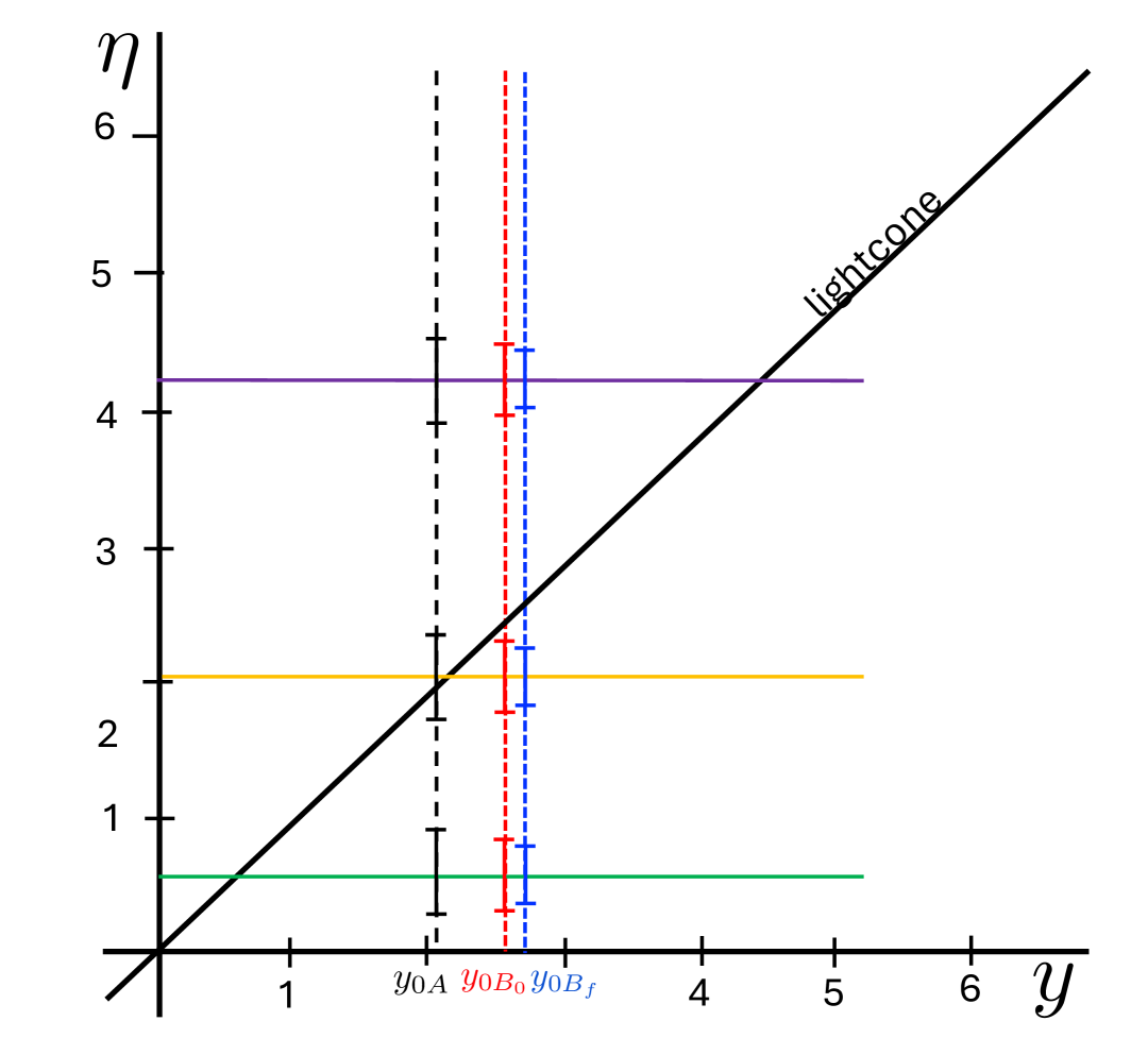
Figure 1: Schematic image of the trajectories swept over to calculate their concurrence. The trajectory $X_{A}$ was kept at fixed $y_{0A}$, while that for $X_{B}$ was swept from $y_{0B_{0}}$ (red) to $y_{0B_{f}}$ (blue). The supports of the switching functions were studied in three separate cases, above (purple), at (orange), and below (green) the lightcone. These supports are shown with bolder lines.

Some other parameter values of note are:

• The parameter that controls the deformation of the quench spacetime in (2): $b=0.5\sigma$

• For the numerical calculations, we set the width of the support of the switching function $\sigma$ to $1$.

The coupling constant $\lambda$ enters $\mathcal{L}_{ij}$ (18) and $\mathcal{M}$ (19) only as the overall multiplicative factor $\lambda^{2}$. The concurrence (26) is hence proportional to $\lambda^{2}$. The concurrence plots in Figures 3–5 give the concurrence divided by $\lambda^{2}$ and are hence independent of $\lambda$. The mutual information (III.4) is by construction independent of $\lambda$. The value of $\lambda$ does therefore not appear in our results.

IV.2 Setup for Mutual Information Calculation

We compute the mutual information (III.4) as a function of the energy gap $\Omega$ and the position of detector B, $\chi_{B}$, in the same three scenarios as before: before, at, and after the pulse of the SET; a depiction of the setting is again given in Figure 1.

The ranges over which the energy gap $\Omega$ and the position of detector $B$ were varied were adjusted from those used in the concurrence calculations, in order to focus on the region of the plot where the mutual information exhibited its most salient features. The specific values used are listed in Table 3.

	Min Value	Max Value
$\Omega$	$-5/\sigma$	$15/\sigma$
$\chi_{B0}$	$3.05\sigma$	$4.0\sigma$
$y_{B0}$	$2.51$	$2.78$

Table 3: Range of values over which we calculated the mutual information, expressed in terms of the duration of the interaction, $\sigma$.

V Results

V.1 Concurrence

Density plots of the concurrence calculated as a function of the energy gap, $\Omega$, and the initial position of detector $B$, $\chi_{B}$, are shown in figures 3, 3 and 5. Figure 3 corresponds to the case where the detectors interact before the SET pulse, Figure 3 to the case where they interact at the pulse, and Figure 5 corresponds to the case where they interact after the pulse.

For comparison, Figure 5 shows the concurrence for a pair of detectors in Rindler spacetime in the Minkowski vacuum, with the corresponding parameter values.

From the figures we observe that the entanglement harvested when the two detectors operate before the SET pulse or after the SET pulse is very similar to the entanglement harvested in Rindler spacetime. When the detectors operate at the SET pulse, however, the entanglement harvested shows a small but distinct increase.

In all the figures we see that the entanglement harvested peaks with an energy gap between $13/\sigma$ and $16/\sigma$ depending on the separation between the detectors. Also, for all values of $\Omega$ the concurrence decreases as we separate the detectors.

V.2 Mutual Information

The density plots of the mutual information as a function of the energy gap, $\Omega$, and the initial position of detector $B$, $\chi_{B0}$ are shown in figures 7, 7, and 8, corresponding to the cases of below, at, and above the SET pulse, respectively.

When the two detectors are operating before the SET pulse or after the SET pulse, the plots are closely are similar. When the detectors operate at the SET pulse, however, the mutual information shows a small but distinct increase.

All three figures show a similar dependence of the mutual information in terms of the energy gap, $\Omega$, and the position of detector $B$, $\chi_{B0}$. Mutual information peaks around an energy gap of $4/\sigma$ for all values of $\chi_{B0}$. Also, for all values of $\Omega$ plotted, the mutual information decreases as we separate the detectors.

VI Conclusions

Motivated by the proposal of [37, 38] to simulate the Unruh effect experimentally with ultracold fermionic atoms in an optical lattice, by a rapid quench in the dispersion relation, we have analysed the entanglement of a scalar field in a similar $(1+1)$-dimensional continuum quench spacetime, and the harvesting of this entanglement by a pair of Unruh-DeWitt detectors. We found that the concurrence and mutual information harvested by the pair of detectors are indeed qualitatively similar to those in Rindler spacetime, but they are slightly yet distinctly higher when the energy pulse created by the quench crosses the detectors’ worldlines.

Our results strongly suggest that entanglement is present also in the optical lattice setup of [37, 38], and raise the possibility that entanglement harvesting could be experimentally realised there. Our results hence provide a further rationale to realise the experimental proposal of [37, 38].

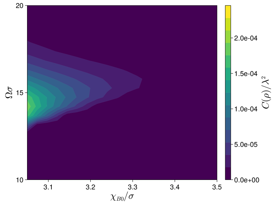
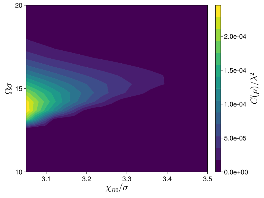
Figure 2: Concurrence obtained by detectors interacting below the SET pulse, as a function of $\Omega$ and initial position of detector B, $\chi_{B0}$.

Figure 3: Concurrence obtained by detectors interacting at the SET pulse, as a function of $\Omega$ and initial position of detector B, $\chi_{B0}$.

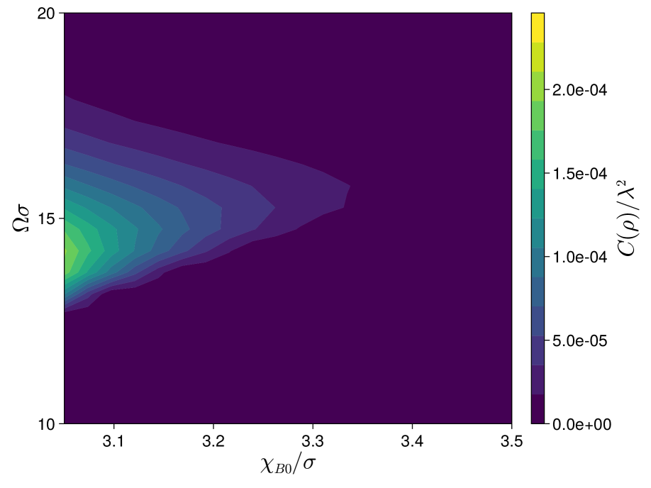
Figure 4: Concurrence obtained by detectors interacting above the SET pulse, as a function of $\Omega$ and initial position of detector B, $\chi_{B0}$.

Figure 5: Concurrence obtained by accelerated detectors in flat 2d Minkowski, as a function of $\Omega\sigma$ and initial position/acceleration of detector B, $\chi_{B0}\sigma$.

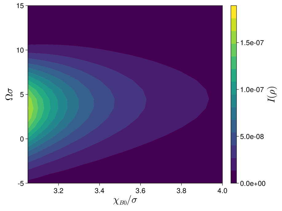
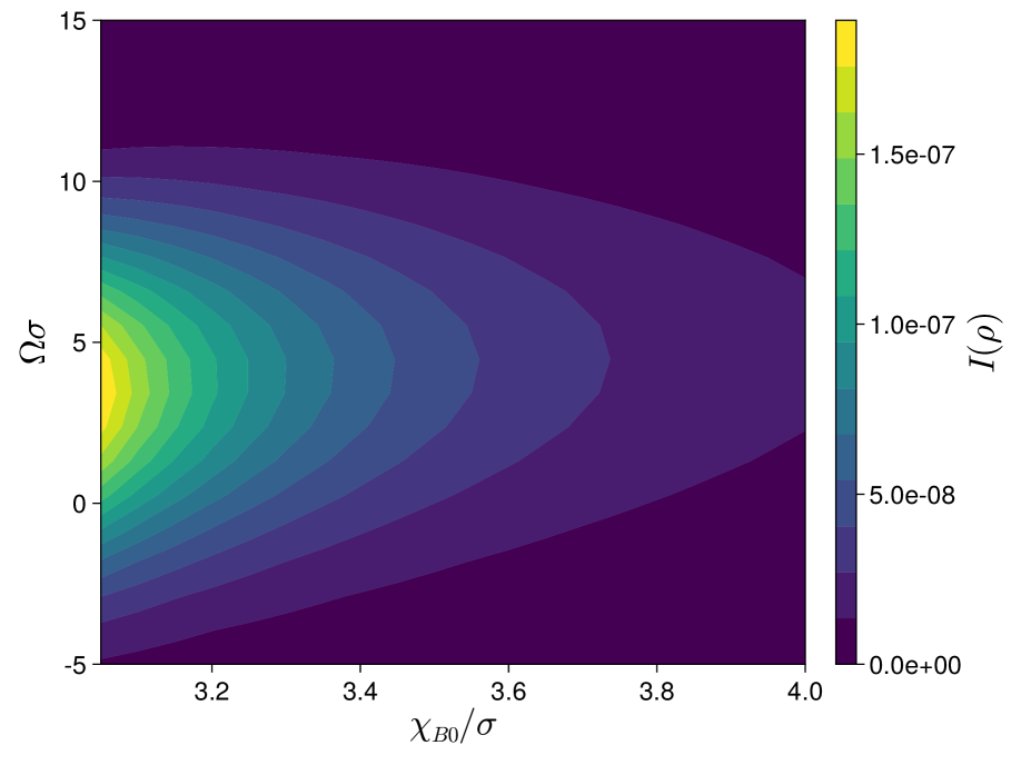
Figure 6: Mutual Information obtained by detectors interacting below the SET pulse, as a function of $\Omega$ and initial position of detector B, $\chi_{B0}$.

Figure 7: Mutual Information obtained by detectors interacting at the SET pulse, as a function of $\Omega$ and initial position of detector B, $\chi_{B0}$.

Figure 8: Mutual Information obtained by detectors interacting above the SET pulse, as a function of $\Omega$ and initial position of detector B, $\chi_{B0}$.

Appendix A About the Code used for the Calculations

The code used for the calculation is publicly available at:
publicly https://github.com/khalil753/quench/
It is designed to be as reusable as possible for future entanglement harvesting projects. For any questions about the structure or operation of the code, please email Adrian at a22lopez@uwaterloo.ca or alopezraven@perimeterinstitute.ca.

The code basically consists of a series of functions that lead up to the calculation of expressions (18) and (19) using numerical integration, after which the density matrix may be determined through (17), from which the concurrence can be immediately calculated.

A.1 Validation of the Code

Given that the entanglement harvesting results calculated in this project have no analytical results or experimental data against which to compare/verify them, to guarantee a certain degree of reliability of our results, we used the same code to calculate properties of other spacetimes which have been previously calculated in the literature so as to make sure we could reproduce them, therefore providing some trust in our numerical calculations. More specifically we:

1. Calculated the reduced density matrix elements of an inertial trajectory in 4d flat spacetime, with gaussian switching function, coupled to a massless free scalar; we plotted these results against the separation of the detectors and against their energy gap, and compared these results to the ones calculated analytically in [51]. Our numerical calculations perfectly matched the analytical results found in [51].

2. We calculated the entanglement harvested by accelerated detectors in 4d flat spacetime and compared our results to those obtained also numerically in [52]. Again, we found perfect agreement with their results.

3. We calculated the entanglement harvested in the quench spacetime in the limit of $b$ going to zero (i.e. the limit in which one should recover accelerated trajectories in flat spacetime) with fixed $\sigma$, and we calculated the entanglement harvest by accelerated trajectories in flat spacetime finding that the two coincided.

References

- [1] S. J. Summers and R. Werner, The vacuum violates Bell’s inequalities, Phys. Lett. 110A (1985), no. 5 257 – 259.
- [2] S. J. Summers and R. Werner, Bell’s inequalities and quantum field theory. I. General setting, J. Math. Phys. (N.Y.) 28 (1987), no. 10 2440–2447.
- [3] A. Valentini, Non-local correlations in quantum electrodynamics, Phys. Lett. 153A (1991), no. 6 321 – 325.
- [4] B. Reznik, Entanglement from the vacuum, Found. Phys. 33 (2003), no. 1 167–176.
- [5] B. Reznik, A. Retzker, and J. Silman, Violating Bell’s inequalities in vacuum, Phys. Rev. A 71 (Apr, 2005) 042104.
- [6] A. Pozas-Kerstjens and E. Martín-Martínez, Harvesting correlations from the quantum vacuum, Phys. Rev. D 92 (Sep, 2015) 064042.
- [7] J. Doukas and B. Carson, Entanglement of two qubits in a relativistic orbit, Phys. Rev. A 81 (Jun, 2010) 062320.
- [8] G. Salton, R. B. Mann, and N. C. Menicucci, Acceleration-assisted entanglement harvesting and rangefinding, New J. Phys. 17 (mar, 2015) 035001.
- [9] J. Zhang and H. Yu, Entanglement harvesting for Unruh-DeWitt detectors in circular motion, Phys. Rev. D 102 (Sep, 2020) 065013.
- [10] Z. Liu, J. Zhang, and H. Yu, Entanglement harvesting in the presence of a reflecting boundary, J. High Energy Phys. 08 (2021), no. 2021 020.
- [11] Z. Liu, J. Zhang, R. B. Mann, and H. Yu, Does acceleration assist entanglement harvesting?, Phys. Rev. D 105 (2022), no. 8 085012.
- [12] J. Foo, S. Onoe, and M. Zych, Unruh-deWitt detectors in quantum superpositions of trajectories, Phys. Rev. D 102 (Oct, 2020) 085013.
- [13] C. Suryaatmadja, R. B. Mann, and W. Cong, Entanglement harvesting of inertially moving Unruh-DeWitt detectors in Minkowski spacetime, Phys. Rev. D 106 (Oct, 2022) 076002.
- [14] Z. Liu, J. Zhang, and H. Yu, Entanglement harvesting of accelerated detectors versus static ones in a thermal bath, Phys. Rev. D 107 (Feb, 2023) 045010.
- [15] M. Naeem, K. Gallock-Yoshimura, and R. B. Mann, Mutual information harvested by uniformly accelerated particle detectors, Phys. Rev. D 107 (Mar, 2023) 065016.
- [16] G. V. Steeg and N. C. Menicucci, Entangling power of an expanding universe, Phys. Rev. D 79 (Feb, 2009) 044027.
- [17] M. Cliche and A. Kempf, Vacuum entanglement enhancement by a weak gravitational field, Phys. Rev. D 83 (Feb, 2011) 045019.
- [18] E. Martín-Martínez, A. R. H. Smith, and D. R. Terno, Spacetime structure and vacuum entanglement, Phys. Rev. D 93 (Feb, 2016) 044001.
- [19] S. Kukita and Y. Nambu, Harvesting large scale entanglement in de Sitter space with multiple detectors, Entropy 19 (Aug, 2017) 449.
- [20] L. J. Henderson, R. A. Hennigar, R. B. Mann, A. R. H. Smith, and J. Zhang, Harvesting entanglement from the black hole vacuum, Classical Quantum Gravity 35 (oct, 2018) 21LT02.
- [21] K. K. Ng, R. B. Mann, and E. Martín-Martínez, Unruh-DeWitt detectors and entanglement: The anti–de Sitter space, Phys. Rev. D 98 (Dec, 2018) 125005.
- [22] L. J. Henderson, R. A. Hennigar, R. B. Mann, A. R. Smith, and J. Zhang, Entangling detectors in anti-de Sitter space, J. High Energy Phys. 05 (2019), no. 2019 178.
- [23] W. Cong, C. Qian, M. R. Good, and R. B. Mann, Effects of horizons on entanglement harvesting, J. High Energy Phys. 10 (Oct, 2020) 67.
- [24] M. P. G. Robbins, L. J. Henderson, and R. B. Mann, Entanglement amplification from rotating black holes, Classical Quantum Gravity 39 (2022), no. 2 02LT01.
- [25] Q. Xu, S. Ali Ahmad, and A. R. H. Smith, Gravitational waves affect vacuum entanglement, Phys. Rev. D 102 (Sep, 2020) 065019.
- [26] E. Tjoa and R. B. Mann, Harvesting correlations in Schwarzschild and collapsing shell spacetimes, J. High Energy Phys. 08 (2020), no. 2020 155.
- [27] K. Gallock-Yoshimura, E. Tjoa, and R. B. Mann, Harvesting entanglement with detectors freely falling into a black hole, Phys. Rev. D 104 (Jul, 2021) 025001.
- [28] F. Gray, D. Kubizňák, T. May, S. Timmerman, and E. Tjoa, Quantum imprints of gravitational shockwaves, J. High Energy Phys. 11 (2021), no. 2021 054.
- [29] K. Bueley, L. Huang, K. Gallock-Yoshimura, and R. B. Mann, Harvesting mutual information from BTZ black hole spacetime, Phys. Rev. D 106 (Jul, 2022) 025010.
- [30] L. J. Henderson, S. Y. Ding, and R. B. Mann, Entanglement harvesting with a twist, AVS Quantum Science 4 (2022), no. 1 014402.
- [31] J. G. A. Caribé, R. H. Jonsson, M. Casals, A. Kempf, and E. Martín-Martínez, Lensing of vacuum entanglement near Schwarzschild black holes, Phys. Rev. D 108 (Jul, 2023) 025016.
- [32] I.-C. Benea-Chelmus, F. F. Settembrini, G. Scalari, and J. Faist, Electric field correlation measurements on the electromagnetic vacuum state, Nature 568 (2019) 202–206.
- [33] F. F. Settembrini, F. Lindel, A. M. Herter, S. Y. Buhmann, and J. Faist, Detection of quantum-vacuum field correlations outside the light cone, Nature Communications 13 (2022) 3383.
- [34] F. Lindel, A. M. Herter, J. Faist, and S. Y. Buhmann, Probing vacuum field fluctuations and source radiation separately in space and time, Phys. Rev. Res. 5 (2023), no. 4 043207.
- [35] F. Lindel, A. Herter, V. Gebhart, J. Faist, and S. Y. Buhmann, Entanglement harvesting from electromagnetic quantum fields, Phys. Rev. A 110 (Aug, 2024) 022414.
- [36] C. Gooding, A. Sachs, R. B. Mann, and S. Weinfurtner, Vacuum entanglement probes for ultra-cold atom systems, New J. Phys. 26 (2024), no. 10 105001.
- [37] J. Rodríguez-Laguna, L. Tarruell, M. Lewenstein, and A. Celi, Synthetic Unruh effect in cold atoms, Phys. Rev. A 95 (Jan, 2017) 013627.
- [38] A. Kosior, M. Lewenstein, and A. Celi, Unruh effect for interacting particles with ultracold atoms, SciPost Phys. 5 (2018) 061.
- [39] J. Louko, Thermality from a Rindler quench, Classical and Quantum Gravity 35 (sep, 2018) 205006.
- [40] W. G. Unruh, Notes on black-hole evaporation, Phys. Rev. D 14 (Aug, 1976) 870–892.
- [41] B. S. DeWitt, Quantum gravity: The new synthesis, in General Relativity: An Einstein Centenary Survey (S. W. Hawking and W. Israel, eds.), pp. 680–745, Cambridge University Press, 1979.
- [42] B. A. Juárez-Aubry and J. Louko, Onset and decay of the 1+1 Hawking-Unruh effect: What the derivative-coupling detector saw, Classical and Quantum Gravity 31 (nov, 2014) 245007.
- [43] B. A. Juárez-Aubry and J. Louko, Quantum fields during black hole formation: How good an approximation is the Unruh state?, J. High Energy Phys. 05 (May, 2018) 140.
- [44] E. Martín-Martínez and P. Rodriguez-Lopez, Relativistic quantum optics: The relativistic invariance of the light-matter interaction models, Phys. Rev. D 97 (May, 2018) 105026.
- [45] E. Martín-Martínez, T. R. Perche, and B. de S. L. Torres, General relativistic quantum optics: Finite-size particle detector models in curved spacetimes, Phys. Rev. D 101 (Feb, 2020) 045017.
- [46] W. K. Wootters, Entanglement of Formation of an Arbitrary State of Two Qubits, Phys. Rev. Lett. 80 (Mar, 1998) 2245–2248.
- [47] M. Nielsen and I. Chuang, Quantum Computation and Quantum Information. Cambridge Series on Information and the Natural Sciences. Cambridge University Press, Cambridge, England, 2000.
- [48] M. Horodecki, P. Horodecki, and R. Horodecki, Separability of mixed states: necessary and sufficient conditions, Phys. Lett. A 223 (1996), no. 1 1–8.
- [49] H. Ollivier and W. H. Zurek, Quantum discord: A measure of the quantumness of correlations, Phys. Rev. Lett. 88 (Dec, 2001) 017901.
- [50] L. Henderson and V. Vedral, Classical, quantum and total correlations, J. Phys. A 34 (aug, 2001) 6899–6905.
- [51] Smith, Alexander R. H., Detectors, Reference Frames, and Time. PhD thesis, University of Waterloo, 2017.
- [52] Z. Liu, J. Zhang, and H. Yu, Entanglement harvesting of accelerated detectors versus static ones in a thermal bath, Phys. Rev. D 107 (Feb, 2023) 045010.