Stellar Mass Segregation in Dark Matter Halos

Abstract

We study the effect of stellar mass segregation driven by collisional relaxation within the potential well of a smooth dark matter halo. This effect is of particular relevance for old stellar systems with short crossing times, where small collisional perturbations accumulate over many dynamical time scales. We run collisional $N$-body simulations tailored to the ambiguous stellar systems Ursa Major 3/Unions 1, Delve 1 and Eridanus 3, modelling their stellar populations as two-component systems of high- and low-mass stars, respectively. For Ursa Major 3/Unions 1 (Delve 1), assuming a dynamical-to-stellar mass ratio of 10, we find that after 10 Gyr of evolution, the radial extent of its low-mass stars will be twice as large (40 per cent larger) than that of its high-mass stars. We show that weak tides do not alter this relative separation of half-light radii, whereas for the case of strong tidal fields, mass segregation facilitates the tidal stripping of low-mass stars. We further find that as the population of high-mass stars contracts and cools, the number of dynamically formed binaries within that population increases. Our results call for caution when using stellar mass segregation as a criterion to separate star clusters from dwarf galaxies, and suggest that mass segregation increases the abundance of massive binaries in the central regions of dark matter-dominated dwarf galaxies.

1 Introduction

In cold dark matter cosmology, galaxies are expected to form deep within the potential wells of dark matter halos (White & Rees, 1978). Numerical simulations suggest that these cold dark matter halos reach remarkably high central densities, well-described by a universal centrally-divergent density profile (Navarro et al., 1996, 1997). The centrally-divergent centers of cold dark matter halos are commonly referred to as “cusps”. Density cusps render cold dark matter halos resilient to the effect of tides (Peñarrubia et al., 2010; van den Bosch et al., 2018): for a fixed tidal field strength, it is argued that cold dark matter halos cannot be tidally stripped beyond a certain point and instead converge towards a stable asymptotic remnant state (Errani & Navarro, 2021; Stücker et al., 2023). Stars embedded in such cold dark matter cusps would be protected from tidal disruption, plausibly giving rise to a population of “micro galaxies” (Errani & Peñarrubia, 2020; Errani et al., 2024a). The discovery of such objects would allow to put strong constraints on the nature of dark matter, as discussed in the context of a potential self-annihilation signal (Crnogorčević & Linden, 2024; Errani et al., 2024b), primordial black hole dark matter (Graham & Ramani, 2024) or ultra-light particle dark matter (Safarzadeh & Spergel, 2020).

In recent years, deep photometric surveys have led to the discovery of several objects with structural parameters at the interface of the globular cluster- and dwarf galaxy regimes (Conn et al., 2018; Mau et al., 2020; Cerny et al., 2023a, b; Smith et al., 2024). Could some of these systems possibly be among the faintest yet dark matter-dominated dwarf galaxies known to date (Errani et al., 2024b; Smith et al., 2024; Simon et al., 2024)? Proving unequivocally that these objects are either dark matter-dominated dwarf galaxies or star clusters devoid of any dark matter has been proven a highly challenging task.

Traditionally, stellar kinematics have been used to argue in favor of the high dark matter content of dwarf galaxies (Mateo, 1998; Walker et al., 2007). For faint stellar systems with few member stars, the inferred velocity dispersions are shown to sensitively depend on the inclusion- or exclusion of individual members stars (Smith et al., 2024) and the choice of prior (Simon et al., 2024). The presence of binary stars further complicates such studies by adding a velocity dispersion floor that, in particular for low-mass dwarf galaxies, needs to be accurately accounted for and generally requires the availability of multi-epoch spectroscopic measurements (McConnachie & Côté, 2010; Buttry et al., 2022).

Another pathway suggested to distinguish dwarf galaxies from globular clusters has been to use the element abundance patterns of their stars (see e.g. Gratton et al. 2012, Bastian & Lardo 2018 for a discussion of element abundances in globular clusters, and Venn et al. 2004, Ji et al. 2019 for dwarf galaxies), though their application to faint stellar systems with few member stars remains challenging (Zaremba et al., 2025).

A further strategy discussed in the literature is based on tidal survival: the existence of the ancient stellar system Ursa Major 3/Unions 1 (Smith et al., 2024) in the inner region of the Milky Way has been used to argue in favour of it being embedded in a dark matter halo and in turn protected from tidal disruption (Errani et al., 2024b). This picture though has been recently challenged by Devlin et al. (2025) who argue that the baryonic mass of Ursa Major 3/Unions 1 has been underestimated in its discovery paper, making it more stable against Milky Way tides even in absence of a surrounding dark matter halo.

Yet another method to distinguish dark matter-dominated objects from those without dark matter has been to search for observational signatures of collisional and collisionless dynamics. The canonical picture is that in dark matter-dominated systems, stellar orbits are determined by the (dark matter) mean field and obey the collisionless Boltzmann equation. Hence, particle-mesh (Fellhauer et al., 2000) and tree codes with force softening (Springel, 2005) have been employed for their study. For globular clusters instead, the importance of close stellar encounters is thought to play an important role in shaping their complex dynamical evolution (Spitzer, 1987), with direct $N$-body codes being necessary for their study (Aarseth, 1999). A prominent signature of collisional processes is the segregation of stellar masses, which has been discussed also in the context of the nature of faint stellar systems (Kim et al., 2015; Baumgardt et al., 2022; Simon et al., 2024; Zaremba et al., 2025) and as a potential means to constrain the progenitors of tidal streams with seemingly conflicting dynamical and chemical signatures (Errani et al., 2022).

In this work, we challenge the canonical picture that dark matter-dominated systems do not show signatures of collisional processes. Taking the ambiguous stellar systems Ursa Major 3/ Unions 1 (UMa3/U1 for short, stellar mass $M_{\star}=16^{\mathmakebox[width("$^{-}$")][c]{+}6}_{\mathmakebox[width("$^{-}$")][c]{-}5}$, projected half-light radius $R_{\mathrm{h}}=(3\pm 1)\mathrm{pc}$, line-of-sight velocity dispersion $\sigma_{\mathrm{los}}\lesssim 4\,\mathrm{km\,s^{-1}}$, see Smith et al. 2024 and footnote 1), Delve 1 (Del1, $M_{\star}=144^{\mathmakebox[width("$^{-}$")][c]{+}24}_{\mathmakebox[width("$^{-}$")][c]{-}27}$, $R_{\mathrm{h}}=6.2^{\mathmakebox[width("$^{-}$")][c]{+}1.5}_{\mathmakebox[width("$^{-}$")][c]{-}1.1}\,\mathrm{pc}$, $\sigma_{\mathrm{los}}\lesssim 5\,\mathrm{km\,s^{-1}}$ see Mau et al. 2020, Simon et al. 2024 and footnote 1) and Eridanus 3 (Eri3, $M_{\star}=800^{\mathmakebox[width("$^{-}$")][c]{+}470}_{\mathmakebox[width("$^{-}$")][c]{-}300}$, $R_{\mathrm{h}}=8.6^{\mathmakebox[width("$^{-}$")][c]{+}0.9}_{\mathmakebox[width("$^{-}$")][c]{-}0.8}\,\mathrm{pc}$, $\sigma_{\mathrm{los}}\lesssim 1\,\mathrm{km\,s^{-1}}$, see Conn et al. 2018, Simon et al. 2024 and footnotes 1 and 1) as examples, we run collisional $N$-body simulations where we assume that these systems are dark matter-dominated and deeply embedded in a smooth dark matter halo. We will show that, driven by their short crossing times, small collisional perturbations due to the minute potential fluctuations caused by their own stars’ gravity can sum up over many gigayears and influence their dynamical evolution. Specifically, for UMa3/U1 and Del1, we show that signatures of mass segregation can be observed even for dynamical-to-stellar mass ratios as high as ${\sim}50$ and ${\sim}20$, respectively.

The paper is structured as follows. In section 2, we estimate the time scale for collisional relaxation in presence of a smooth dark matter halo. In section 3, we detail the numerical setup of our collisional $N$-body simulations. In section 4.1, we discuss the results of our simulations for the case of a static dark matter halo surrounding each stellar system, and describe the dynamical formation of stellar binaries in Sec. 4.2. We extend our analysis to include the effects of tides through a time-evolving dark matter potential in section 4.4. Finally, we summarize our results and conclusions in section 5.

2 Relaxation Times

The faint stellar systems UMa3/U1, Del1 and Eri3 host ancient stellar populations, with isochrone fits suggesting stellar ages beyond $10\,\mathrm{Gyr}$. For such old systems, it seems plausible that small dynamical perturbations may accumulate over time and give rise to some secular evolution. As we will show in the following, this idea holds even if the stellar population is embedded in a dark matter potential.

If the stellar contribution to the total potential is fully negligible and the dark matter potential is smooth, then the system obeys the Collisionless Boltzmann Equation and, in absence of other perturbations, no secular evolution occurs. However, one may image a system where the stellar contribution to the potential becomes relevant for its dynamical evolution by providing a noisy, fluctuating component to the potential. To illustrate the relevant time scales at play, we will now estimate the time scale for collisional relaxation due to gravitational encounters between stars in presence of a smooth dark matter potential.

We call $M_{\mathrm{h}}=M_{\mathrm{sub}}({<}r_{\mathrm{h}})+M_{\star}({<}r_{\mathrm{h}})$ the total dynamical mass enclosed within the (3D) stellar half-light radius $r_{\mathrm{h}}$, which is the sum of the dark matter subhalo mass $M_{\mathrm{sub}}({<}r_{\mathrm{h}})$ and the stellar mass $M_{\star}({<}r_{\mathrm{h}})=M_{\star}/2$. For short, we will refer to the average dynamical-to-stellar mass ratio within $r_{\mathrm{h}}$ as

$$\Upsilon_{\mathrm{dyn}}\equiv M_{\mathrm{h}}/M_{\star}({<}r_{\mathrm{h}})~.$$ (1)

The stellar component has a (3D) velocity dispersion of roughly $\langle v^{2}\rangle\approx GM_{\mathrm{h}}/r_{\mathrm{h}}=GM_{\star}\Upsilon_{\mathrm{dyn}}/(2r_{\mathrm{h}})$, and a crossing time of

$$T_{\mathrm{cross}}=r_{\mathrm{h}}^{3/2}\left(GM_{\mathrm{h}}\right)^{-1/2}=\sqrt{2/G}~r_{\mathrm{h}}^{3/2}\left(M_{\star}\Upsilon_{\mathrm{dyn}}\right)^{-1/2}~.$$ (2)

For the case of UMa3/U1, for example, we find $T_{\mathrm{cross}}\approx 13\,\mathrm{Myr}$ when assuming a dynamical-to-stellar mass ratio $\Upsilon_{\mathrm{dyn}}=10$: over $10\,\mathrm{Gyr}$, the system has gone through close to ${\sim}800$ crossing times. Over one crossing time, the average squared velocity increase that an individual star experiences due to the fluctuating gravitational potential of $N_{\star}$ stars with individual masses $m_{\star}$ can be approximated by (using Eq. 18 in Peñarrubia 2019 and assuming that the stellar number density $\bar{n}=3N_{\star}/(8\pi r_{\mathrm{h}}^{3})$ is approximately constant within the half-light radius):

$$\langle\Delta v^{2}\rangle_{t=T_{\mathrm{cross}}}/\langle v^{2}\rangle \approx \sqrt{24\pi}~\Upsilon_{\mathrm{dyn}}^{-2}N_{\star}^{-1}\left[\ln(\Lambda)-1.9\right]$$ (3)

$$= \sqrt{3\pi/2}~M_{\mathrm{h}}^{-2}N_{\star}m_{\star}^{2}\left[\ln(\Lambda)-1.9\right]$$ (4)

where $v\approx\langle v^{2}\rangle^{1/2}$ is the velocity of a star, and $\ln(\Lambda)$ is the Coulomb logarithm. From Eq. 3 wee see that, all else equal, $\langle\Delta v^{2}\rangle$ decreases as $\Upsilon_{\mathrm{dyn}}$ and $N_{\star}$ increase: for $\Upsilon_{\mathrm{dyn}}\rightarrow\infty$ and $N_{\star}\rightarrow\infty$, the system becomes collisionless.

As time progresses, these $\langle\Delta v^{2}\rangle$ accumulate. The orbital motion of a star is driven by the potential fluctuations once $\langle\Delta v^{2}\rangle/\langle v^{2}\rangle\approx 1$, which happens over the course of a relaxation time

$$T_{\mathrm{rel}} \approx 1/\sqrt{12\pi G}\,\left(\Upsilon_{\mathrm{dyn}}r_{\mathrm{h}}\right)^{3/2}N_{\star}M_{\star}^{-1/2}\left[\ln(\Lambda)-1.9\right]^{-1}$$ (5)

$$= \sqrt{2/(3\pi G)}\,\left(M_{\mathrm{h}}r_{\mathrm{h}}\right)^{3/2}N_{\star}^{-1}m_{\star}^{-2}\left[\ln(\Lambda)-1.9\right]^{-1}.$$ (6)

All else being equal, the more dark-matter dominated the system is, the larger is its relaxation time.

For a population of stars with a mass function $\mathrm{d}N_{\star}/\mathrm{d}m_{\star}$, the relaxation time will be driven by those stars that maximize the change in $\langle\Delta v^{2}\rangle$: Eq. 4 shows that contribution peaks for stars of a stellar mass $m_{\star}$ that maximizes the product $m_{\star}^{2}\mathrm{d}N_{\star}/\mathrm{d}m_{\star}$. For a Chabrier (2003) present-day mass function, stars with masses $0.4\lesssim m_{\star}/\mathrm{M_{\odot}}\lesssim 1.4$ contribute $68$ per cent of the total $\langle\Delta v^{2}\rangle$. More massive stars do not play much of a role by virtue of their low abundance, while less massive stars do not contribute much by virtue of their mass.

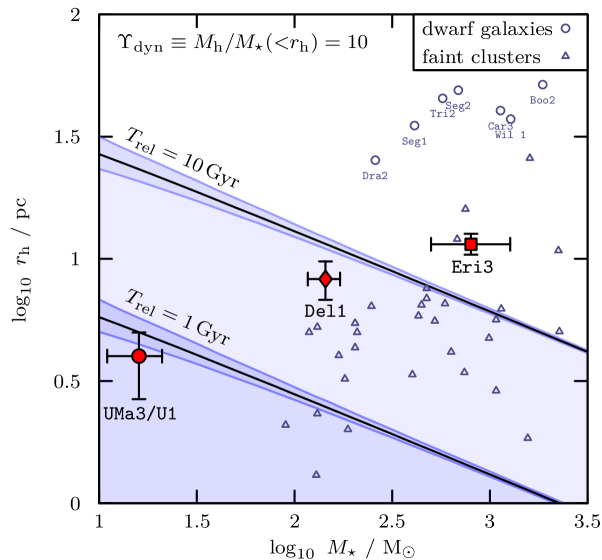
Figure 1: Several Milky Way satellites have relaxation times $T_{\mathrm{rel}}$ smaller than $10\,\mathrm{Gyr}$ even in presence of substantial amounts of dark matter. Those objects may exhibit stellar mass segregation driven by collisional relaxation. Shown are stellar masses $M_{\star}$ and (3D) half-light radii $r_{\mathrm{h}}$ of dwarf galaxies (open circles), ambiguous stellar clusters (triangles), as well as the “micro galaxy” candidates UMa3/U1, Del1 and Eri3 (red filled circle, diamond and square, respectively). See footnote 4 for references. Curves of constant relaxation time $T_{\mathrm{rel}}=1\,\mathrm{Gyr}$ and $10\,\mathrm{Gyr}$ are computed assuming a dynamical-to-stellar mass ratio of $\Upsilon_{\mathrm{dyn}}=10$ within the half-light radius, with stellar masses sampled from a Chabrier (2003) present-day mass function (see text for details).

In Fig. 1, we show Relaxation times computed by summing Eq. 4 over individual stellar masses $m_{\star}$ drawn from a Chabrier (2003) present-day mass function (PDMF), together with a compilation of stellar masses $M_{\star}$ and (3D) half-light radii $r_{\mathrm{h}}$ of Milky Way dwarf galaxies and faint clusters with structural properties at the interface of the globular cluster- and dwarf galaxy regimes. In Fig. 1, we assume $\Upsilon_{\mathrm{dyn}}=10$, but the results are easily translated to other choices for dynamical-to-stellar mass ratio through Eq. 5. Uncertainties on the relaxation times shown here stem from sampling the stellar mass function and span the $16^{\mathrm{th}}$ to $84^{\mathrm{th}}$ percentile of crossing times for random realizations of total mass $M_{\star}$.

For the faint stellar systems UMa3/U1 and Delve1, assuming a dynamical-to-stellar mass ratio of $\Upsilon_{\mathrm{dyn}}=10$, we find relaxation times of $0.9$ and $8.4\,\mathrm{Gyr}$, respectively, substantially lower than the age of their stellar populations. For these systems, we can therefore expect dynamical signatures of collisional processes, such as stellar mass segregation, even when embedded in a smooth, static and gravitationally dominant dark matter subhalo.

3 Numerical Setup

To study the observable effects of collisional relaxation on a stellar population embedded in a smooth dark matter subhalo, we perform a series of $N$-body experiments. In the following, we summarize the details of our numerical setup.

3.1 Example systems

We build our $N$-body models to approximately resemble the faint stellar systems UMa3/U1 (Smith et al., 2024), Del1 (Mau et al., 2020) and Eri3 (Conn et al., 2018). These systems are plausible candidates for being the smallest dwarf galaxies known to date, motivated by their kinematics and chemistry (Simon et al., 2024), or by their tidal survival on a low-pericentre orbit (Errani et al., 2024b). Table 1 lists the structural parameters used for our $N$-body models. We estimate the (3D) half-light radii $r_{\mathrm{h}}\approx 4R_{\mathrm{h}}/3$ from the the published projected radii $R_{\mathrm{h}}$. For UMa3/U1 and Del1, we use total stellar masses as published; for Eri3, we estimate the stellar stellar mass from its luminosity, assuming a stellar mass-to-light ratio of $\Upsilon_{\star}=1.4$. This value matches the stellar mass-to-light ratio inferred in Smith et al. (2024) and Mau et al. (2020) for UMa3/U1 and Del1, respectively.

Table 1: Parameters used for the $N$-body models. The table lists the total stellar mass $M_{\star}$ (for the case of Eri3 estimated from its luminosity), the (3D) half-light radius $r_{\mathrm{h}}\approx 4R_{\mathrm{h}}/3$ estimated from the projected $R_{\mathrm{h}}$, and the total number of star particles $N_{\star}$. For reference, we also list the resulting crossing- (Eq. 2) and relaxation times (Eq. 5) assuming $\Upsilon_{\mathrm{dyn}}=10$ and $20$.

model	$M_{\star}/\mathrm{M_{\odot}}$	$r_{\mathrm{h}}/\mathrm{pc}$	$N_{\star}$	for $\Upsilon_{\mathrm{dyn}}=10$ $(20)$
				$T_{\mathrm{cross}}/\mathrm{Myr}$	$T_{\mathrm{rel}}/\mathrm{Gyr}$
UMa3/U1	16tn:1	4tn:1	50	13 (9)	0.9 (2.7)
Del1	144tn:2	8.3tn:2${}^{\text{,}}$tn:3	450	13 (9)	8.4 (24)
Eri3	800tn:4${}^{\text{,}}$tn:5	11.5tn:4	2500	9 (6)	32 (91)

• Smith et al. (2024)

• Mau et al. (2020)

• Simon et al. (2024)

• Conn et al. (2018)

• assuming $\Upsilon_{\star}=1.4$, see footnote 1

3.2 Initial conditions

Stellar masses. For the sake of simplicity, we model the stellar population as a two-component system consisting of low-mass stars of mass $m_{\star}=0.2\,\mathrm{M_{\odot}}$, and of high-mass stars of mass $m_{\star}=0.8\,\mathrm{M_{\odot}}$. Each sub-population contributes half of the total stellar mass $M_{\star}$. Consequently, in our models, the number of low-mass stars is four times higher than the number of high-mass stars. This choice of stellar masses is roughly guided by the Chabrier (2003) present-day mass function, where half of the total stellar mass $M_{\star}$ is contributed by stars with masses below ${\sim}0.5\,\mathrm{M_{\odot}}$, with a median stellar mass of ${\sim}0.2\,\mathrm{M_{\odot}}$. The second half of the total stellar mass is contributed by stars with masses above ${\sim}0.5\,\mathrm{M_{\odot}}$, with a median stellar mass of ${\sim}0.8\,\mathrm{M_{\odot}}$.

Stellar profiles. We assume that, initially, the combined density profile of both low-mass and high-mass stars follows a spherical (3D) exponential profile,

$$\rho_{\star}(r)=M_{\star}/(8\pi r_{\star}^{3})~\exp(-r/r_{\star})~,$$ (7)

where $r_{\star}\approx r_{\mathrm{h}}/2.67$ is the stellar scale radius. Initially, the stellar half-light radii $r_{\mathrm{h}}$ coincide between the two sub-populations. We embed the stellar models deeply within the potential well of a smooth dark matter subhalo: $r_{\mathrm{h}}/r_{\mathrm{sub}}=1/500$, for a dark matter scale radius $r_{\mathrm{sub}}$ defined as follows.

Dark matter profiles. We model the (smooth) dark matter subhalo surrounding the stellar component and centered on it using a spherical Hernquist (1990) profile, with a total mass $M_{\mathrm{sub}}$ and a scale radius $r_{\mathrm{sub}}$,

$$\rho_{\mathrm{sub}}(r)=M_{\mathrm{sub}}/(2\pi r_{\mathrm{sub}}^{3})~(r/r_{\mathrm{sub}})^{-1}(1+r/r_{\mathrm{sub}})^{-3}~.$$ (8)

This dark matter density profile is cuspy, i.e., $\mathrm{d}\ln\rho_{\mathrm{sub}}/\mathrm{d}\ln r\rightarrow-1$ for $r\rightarrow 0$.

$N$-body realizations. We generate equilibrium $N$-body realizations of Eq. 7 in the combined potential of the dark matter and stellar components using using the Eddington-inversion code nbopy (Errani & Peñarrubia, 2020), available online. We assume that both stellar components have isotropic velocities in the initial conditions. The dark matter subhalo (Eq. 8) is modelled as an analytical background potential. To reduce the impact of Poisson noise on our analysis, for each choice of dynamical-to-stellar mass ratio $\Upsilon_{\mathrm{dyn}}$, we generate $200$ realizations of our UMa3/U1 model, $40$ for Del1, and $10$ for Eri3.

3.3 $N$-body code

We compute the time evolution of our $N$-body models using petar (Wang et al., 2020a), a collisional $N$-body code, which in turn builds upon the slow-down arithmetic regularization package sdar (Wang et al., 2020b) and the general-purpose library for particle simulations fdps (Iwasawa et al., 2016; Namekata et al., 2018). petar employs a fourth-order Hermite integrator to handle short-range forces, and a Barnes & Hut (1986) tree for long-range ones. No force softening is used. The analytical Hernquist potential is included in the force calculations by making use of the code’s galpy (Bovy, 2015) interface.

For the UMa3/U1 models, we update the particle tree responsible for the long-range forces with a step size of $\Delta t_{\mathrm{L}}=2^{-10}r_{\mathrm{sub}}^{3/2}(GM_{\mathrm{sub}})^{-1/2}$. With this choice, the period of a circular orbit at the initial half-light radius $r_{\mathrm{h}}/r_{\mathrm{sub}}=1/500$ of a particle that is only subject to long-range forces (including the force due to the analytical dark matter potential) is resolved by ${\approx}270$ steps for the models with $\Upsilon_{\mathrm{dyn}}=10$. To test for numerical convergence, we have decreased and increased this value by factors of 4, with no qualitative impact on our results. Following the recommendation in Wang et al. (2020a, see their Eq. 12 and 41), we choose as reference radii for the separation of short- and long-range forces the values $r_{\mathrm{in,ref}}=\Delta t_{\mathrm{L}}\sigma_{1D}$ and $r_{\mathrm{out,ref}}=10\,r_{\mathrm{in,ref}}$, where by $\sigma_{1D}$ we denote the $N$-body system’s velocity dispersion. Slow-down regularization through sdar is applied to particles below a radius $r_{\mathrm{bin}}=0.8\,r_{\mathrm{in,ref}}$ (the default value in petar). To test for convergence, we have decreased this radius by a factor of 8, again with no qualitative impact on our results.

For the Del1 models, we use the same tree time step and reference radii as for UMa3/U1. Instead for Eri3, we use a shorter tree time step of $\Delta t_{\mathrm{L}}=2^{-12}r_{\mathrm{sub}}^{3/2}(GM_{\mathrm{sub}})^{-1/2}$, which results in better performance at that $N$-body particle number by reducing the number of particles within $r_{\mathrm{in,ref}}$.

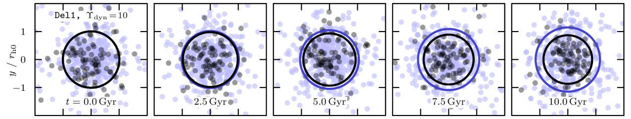
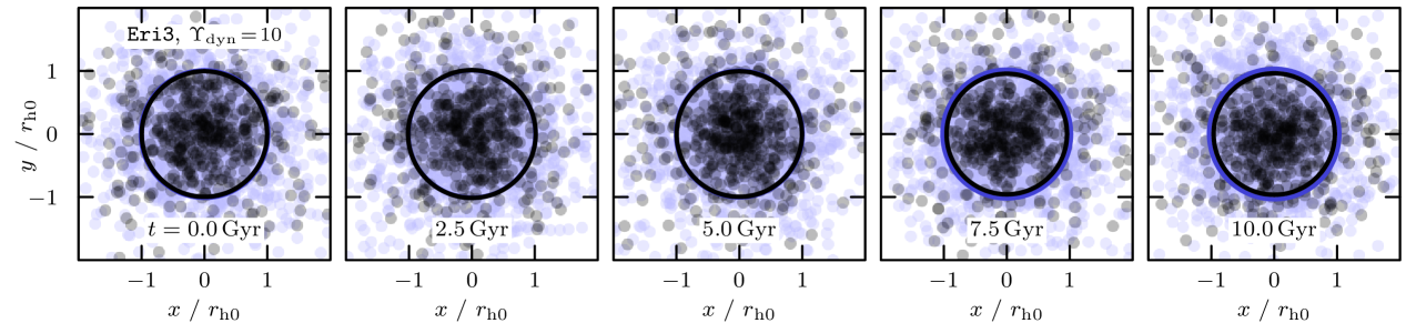
Figure 2: Stellar mass segregation in $N$-body realizations of the example systems UMa3/U1 (top), Del1 (center) and Eri1 (bottom). Each system is embedded in a cuspy dark matter halo, with an initial dynamical-to-stellar mass ratio of $\Upsilon_{\mathrm{dyn}}=10$. Shown are $\{x,y\}$ projections of snapshots at $t/\mathrm{Gyr}=0$, $2.5$, $5$, $7.5$ and $10$. The axes are expressed in units of the initial half-light radius $r_{\mathrm{h0}}$. Individual high-mass stars are shown as dark grey points, while low-mass stars are shown in blue. The median half-light radii of high-mass and low-mass stars (computed over a sample of $N$-body realizations, see text) are shown as black and blue circles, respectively. Over a period of $10\,\mathrm{Gyr}$, the half-light radius of the population of low-mass stars expands, while the half-light radius of the high-mass population contracts. Consistent with the relaxation time estimates of Fig. 1, the effect is largest for the UMa3/U1 model, and smallest for the Eri3 model. Dynamically-formed binaries consisting of two high-mass stars are highlighted in red (see Sec. 4.2). A video version of this figure is available as an arXiv ancillary file.

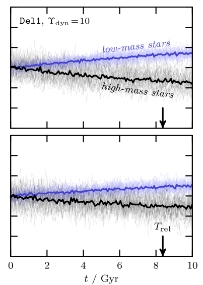
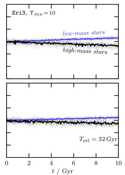
Figure 3: As stellar mass segregation progresses, the half-light radius of the low-mass stars expands as the population heats up, whereas the population of high-mass stars contracts and cools down. The same systems are shown as in Fig. 2, with an initial dynamical-to-stellar mass ratio of $\Upsilon_{\mathrm{dyn}}=10$. Thick blue (black) lines show the median time evolution of the low-mass (high-mass) stellar population computed from all $N$-body realizations (see text), whereas light blue (grey) lines show individual runs. Poisson noise widens the distribution of half-light radii and velocity dispersions, most notably for the case of UMa3/U1 (left) with $N_{\star}=50$ stars.

4 Simulations results

We can now turn our attention to the results of our $N$-body experiments. In Sec. 4.1, we describe the simulations of UMa3/U1, Del1 and Eri3 assuming that the stellar component is embedded in a static dark matter halo. Then, in Sec. 4.4, we model the effect of tides on the system by allowing the underlying dark matter potential to evolve with time.

4.1 Simulations in a static dark matter halo

Figure 2 shows simulation snapshots of the UMa3/U1 (top), Del1 (center) and Eri3 (bottom) models, evolved for $10\,\mathrm{Gyr}$ in a static dark matter halo. These models have an initial dynamical-to-stellar mass ratio of $\Upsilon_{\mathrm{dyn}}=10$ within the (initial) half-light radius. Individual low-mass (high-mass) stars are shown as light-blue (grey) points, respectively. As time progresses, the population of low-mass stars expands, while the population of high-mass stars contracts: Even though the system is highly dark matter-dominated, the stellar population undergoes mass segregation driven by collisional relaxation. Blue and black circles in Figure 2 show the median half-light radii of the low-mass (high-mass) population, with the median computed from the sample of all $N$-body realizations. Mass segregation progresses fastest for UMa3/U1 and slowest for Eri3, consistent with the relaxation times estimated in Fig. 1.

The detailed time evolution of the models with $\Upsilon_{\mathrm{dyn}}=10$ is shown in Fig. 3. The top panels show the evolution of the (median) half-light radii of the populations of low-mass (blue) and high-mass (black) stars. For the case of UMa3/U1, after $10\,\mathrm{Gyr}$ of evolution, the half-light radius of the population of low-mass stars is twice as large as the half-light radius of high-mass stars. For Del1, the difference reduces to ${\sim}40$ per cent, and for Eri3 to ${\sim}10$ per cent. The evolution of individual $N$-body realizations is shown in lighter shades in the background: For systems akin to UMa3/U1, Poisson noise driven by the low number of stars in the system substantially complicates a detection of mass segregation. The bottom panels of Fig. 3 show the evolution of the (3D) stellar velocity dispersion $\langle v^{2}\rangle=\sum v^{2}/N_{\star}$. As the half-light radius of the population of low-mass stars expands, the velocity dispersion heats up. Vice-versa, as the population of high-mass stars contracts, the population cools down.

4.2 Dynamical formation and disruption of binaries

As the population of high-mass stars contracts and cools, we note the dynamical formation of stellar binary systems in our simulations. We identify binaries as pairs of stars with Keplerian binding energy $E_{\mathrm{bin}}<0$ and an orbital period $T_{\mathrm{bin}}$ that is shorter than the (circular) period $T_{\mathrm{com}}$ of the pair’s center of mass within the dark matter subhalo. Expressed in terms of densities, this condition implies that the mean stellar density within the semi-major axis $a_{\mathrm{bin}}$ of a binary exceeds the mean density of the dark halo within a radius equal to that of the binary’s center of mass , i.e $(m_{i}+m_{j})/a_{\mathrm{bin}}^{3}>M_{\mathrm{sub}}({<}r_{\mathrm{com}})/r_{\mathrm{com}}^{3}$, where by $m_{i}$ and $m_{j}$ we denote the masses of the two binary components. We count the number of binaries at each snapshot in the simulation. For better statistics, we stack $2000$ realizations of the UMa3/U1 model with an initial dynamical-to-stellar mass ratio of $\Upsilon_{\mathrm{dyn}}=10$. Note that our initial conditions are created by drawing individual stars from the underlying distribution function; any binaries present in the initial conditions just arise from this random sampling.

Figure 4 shows the binary fraction $f_{\mathrm{bin}}\equiv N_{\mathrm{bin},i}/N_{i}$, defined here as the number $N_{\mathrm{bin},i}$ of high-mass stars that are in binary systems, normalized by the total number of high-mass stars $N_{i}$. A grey band show the binary fraction considering only pairs of two high-mass stars, whereas the blue band corresponds to binaries that consist of a high-mass star and a low-mass star. As the population of high-mass stars contracts and cools due to mass segregation, the number of dynamically formed massive–massive binaries increases. At the same time, as the population of low-mass stars expands and heats up, the number of massive–low mass binaries drops.

Some intuition in the processes driving the formation and disruption of dynamical binaries can be gained from the statistical theory of gravitational capture, developed to estimate the number of gravitationally trapped (mass-less) tracer particles around a point-mass perturber orbiting in a smooth dark matter halo (Peñarrubia, 2023). In our collisional $N$-body simulations, all stars are massive particles, and complicated three- or multi-body interaction between stars and the halo likely contribute to the formation and disruption processes. Nevertheless, as we will show in the following, the statistical theory of gravitational capture provides accurate estimates for the binary fractions found in our simulations. Building upon equation 4 in Peñarrubia (2021), we estimate the binary fraction through

$$f_{\mathrm{bin}}\equiv\frac{N_{\mathrm{bin},i}}{N_{i}}\approx\frac{4\sqrt{3}}{\sqrt{\pi}}\left[G\,(m_{i}+m_{j})\,a_{\mathrm{max}}\right]^{3/2}\frac{N_{j}}{r_{{\mathrm{h}j}}^{3}\langle v^{2}_{j}\rangle^{3/2}}$$ (9)

where $N_{i}$ denotes the number and $m_{i}$ the mass of high-mass stars. Analogously, we denote by $N_{j}$, $m_{j}$, $r_{\mathrm{h}j}$ and $\langle v^{2}_{j}\rangle^{1/2}$ the number, mass, (3D) half-light radius and (3D) velocity dispersion of the field population. For massive–low mass binaries, the field population is the population of low-mass stars. For massive–massive binaries, the field population coincides with the population of massive stars, and we set $N_{j}=N_{i}-1$. The radius $a_{\mathrm{max}}$ here is chosen to be the largest semi-major axis for which the binary identification criterion employed in the simulations holds, assuming a binary located at the half-light radius $r_{\mathrm{h}j}$.

From Eq. 9, we see that the fraction of dynamically formed binaries scales with the (proxy) phase space density of the field population, $\propto N_{j}/(r_{\mathrm{h}j}^{3}\langle v^{2}_{j}\rangle^{3/2})$. The latter increases for the case of massive–massive binaries as the population of high-mass stars contracts and cools; hence, $f_{\mathrm{bin}}$ grows. Vice-versa, the (proxy) phase space density of low-mass stars decreases as the population expands and heats up, and $f_{\mathrm{bin}}$ drops. Dashed curves in Fig. 4 show the evolution of $f_{\mathrm{bin}}$ predicted by Eq. 9, in good agreement with the simulation results.

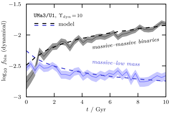
Figure 4: As the population of high-mass stars contracts and cools, the number of dynamically-formed binaries consisting of two massive stars increases. At the same time, as the population of low-mass stars expands and heats up, the number of dynamically-formed binaries consisting of a massive and a low-mass star decreases. Shown is the fraction $f_{\mathrm{bin}}$ of high-mass stars that are in binary systems relative to the total number of high-mass stars. Simulation results are shown as shaded bands, computed from a sample of $2000$ $N$-body realizations of the UMa3/U1 model. Dashed curves show the model predictions of Eq. 9.

4.3 Sensitivity to the dynamical-to-stellar mass ratio

The models described in the previous section assumed an initial dynamical-to-stellar mass ratio of $\Upsilon_{\mathrm{dyn}}=10$. However, Eq. 5 shows that the relaxation time, and hence the effects of collisional processes on the system, depend on the value of $\Upsilon_{\mathrm{dyn}}$. For $\Upsilon_{\mathrm{dyn}}\rightarrow\infty$, the system becomes collisionless, whereas for $\Upsilon_{\mathrm{dyn}}\rightarrow 1$, the dynamics are those of a classical star cluster. To study this dependence on $\Upsilon_{\mathrm{dyn}}$, we run a series of simulations varying the initial dynamical-to-stellar mass ratio over a range of $0.5\leq\log_{10}\Upsilon_{\mathrm{dyn}}\leq 2.5$. Note that we only study models that are dark matter-dominated, as our $N$-body setup does not capture the dynamical effects of stars on the dark matter cusp which would become more relevant as $\Upsilon_{\mathrm{dyn}}$ decreases (see, e.g., Zhang & Amaro Seoane 2025).

In Figure 5, we show the ratio between the half-light radii of the low-mass and high-mass stellar populations after $10\,\mathrm{Gyr}$ of evolution, for different values of the initial dynamical-to-stellar mass ratio $\Upsilon_{\mathrm{dyn}}$. As expected, for large values of $\Upsilon_{\mathrm{dyn}}$, there is no appreciable difference between the half-light radii of the two stellar populations: the system is collisionless. At the other extreme, for $\Upsilon_{\mathrm{dyn}}\sim 3$ and $10\,\mathrm{Gyr}$ of evolution, the stellar half-light radius of the low-mass population is three times, 2 times and 50 per cent larger than that of the population of low-mass stars for the case of the UMa3/U1, Del1 and Eri3 model, respectively. Error bars span the $16^{\mathrm{th}}$ to $84^{\mathrm{th}}$ percentile of the underlying distribution of $N$-body relizations. As before, Poisson noise renders any detection of mass segregation highly challenging for systems with a low number of member stars such as UMa3/U1.

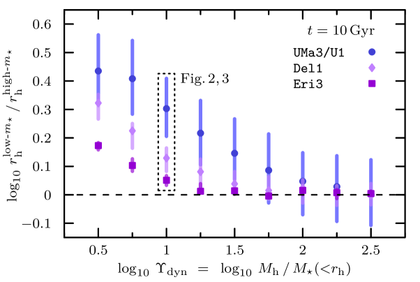
Figure 5: Stellar mass segregation plays a substantial role for the dynamical evolution of systems akin to UMa3/U1 if their dynamical-to-stellar mass ratios $\Upsilon_{\mathrm{dyn}}$ are smaller than ${\sim}50$. Shown is the median ratio of half-light radii between the populations of low-mass and high-mass stars after $10\,\mathrm{Gyr}$ of evolution for different (initial) dynamical-to-stellar mass ratios $\Upsilon_{\mathrm{dyn}}$, computed over all $N$-body realizations (see text). Error bars span the $16^{\mathrm{th}}$ to $84^{\mathrm{th}}$ percentile of the underlying distribution.

4.4 The effect of tides

The simulation results discussed in Sec. 4.1 assume a static dark matter potential surrounding the stellar populations. For the faint stellar systems UMa3/U1, Del1 this assumption is unlikely to hold: located at galactocentric distances similar to that of the sun, these systems will be subject to the tidal field of the Milky Way. For the case of UMa3/U1 on an orbit with a pericentre of $r_{\mathrm{peri}}=13\,\mathrm{kpc}$, a dark matter halo hosting UMa3/U1 could have been tidally stripped to $1/10^{4}$ of its original mass (see Fig. 7 in Errani et al. 2024b).

To model the effect of tides, in the following, we will slowly decrease the mass of the surrounding dark matter halo and adjust its scale radius according to the empirical tidal evolutionary tracks for Hernquist models (see Errani et al. 2018 Table. A1 and Fig. A1 for details). Specifically, we model the evolution of the subhalo total mass as $M_{\mathrm{sub}}/M_{\mathrm{sub0}}=\exp(-t/\tau)$ where $\tau$ is chosen so that over $10\,\mathrm{Gyr}$ of evolution, $M_{\mathrm{sub}}/M_{\mathrm{sub0}}$ decreases to $1/10^{4}$. The scale radius is adjusted through $r_{\mathrm{sub}}/r_{\mathrm{sub0}}\approx(M_{\mathrm{sub}}/M_{\mathrm{sub0}})^{\beta}$ with $\beta=0.48$.

Taking UMa3/U1 as an example, figure 6 shows the results of this experiment. A red curve shows the evolution of the (median) half-light radius $r_{\mathrm{h}}$ and velocity dispersion $\langle v^{2}\rangle^{1/2}$ of the population of low-mass stars, normalized to the respective initial values. A grey curve shows the equivalent evolution for the population of high-mass stars. As previously discussed, the stellar populations mass segregate. Here, in addition, the lowering of the background dark matter potential drives an adiabatic expansion of the stellar components along curves of $r_{\mathrm{h}}\langle v^{2}\rangle^{1/2}=\text{const}$ (black dashed curves, see Errani et al. 2025 for detailed discussion of this adiabatic expansion). Note that, in the size–velocity dispersion plane, the dynamical effects of tides and mass segregation are orthogonal: mass segregation results in an overall expansion and heating (contraction and cooling) of the population of low-mass (high-mass) stars, whereas tides drive an adiabatic expansion and cooling of both components. For the case of the population of high-mass stars, these two processes compete in driving the half-light radius of the stellar population. Crucially, after $10\,\mathrm{Gyr}$ of evolution, the ratio of the half-light radii of the low-mass and high-mass populations are virtually identical between the models which include adiabatic expansion through tides (red and grey lines), and the model run in isolation (blue and dark grey lines). For the case of tidal fields that cause an adiabatic expansion of the stellar component within the power-law cusp of the underlying halo, the ratio of half-light radii shown in Fig. 5 will hence hold independently of whether the system has experienced tides, or not. This finding is consistent with the analytical estimate of the relaxation time in Eq. 6: for constant $N_{\star}$ and $m_{\star}$, the relaxation time scales as $T_{\mathrm{rel}}\propto(M_{\mathrm{h}}r_{\mathrm{h}})^{3/2}$. The product of enclosed mass and half-light radius is approximately conserved during adiabatic expansion, $M_{\mathrm{h}}r_{\mathrm{h}}\propto\langle v^{2}\rangle^{1/2}r_{\mathrm{h}}\approx\text{const}$ (see e.g. Errani et al. 2025 for details). Hence, the relaxation time (Eq. 6) and the binary fraction (Eq. 9) remains virtually unaffected by the adiabatic expansion of the stellar components.

To illustrate the potential landscape and to provide further intuition for the expected evolution in the size–velocity dispersion plane, black curves show the velocity dispersion of a tracer population subject to the combined potential of dark matter and stars, as computed from the Virial theorem (see e.g. Amorisco & Evans 2012, Errani et al. 2018). This simple calculation accurately predicts the velocity dispersion of the mass-segregated populations.

The model for tides employed here does not account for any stellar mass loss, but merely models the response of the stars to the evolving background potential. This is a modelling choice motivated by the fact that asymptotic remnant state (Errani & Navarro, 2021) of a cold dark matter halo on the orbit of UMa3/U1 has a tidal radius that is substantially larger than the half-light radius of UMa3/U1. For stronger tidal fields that result in the tidal stripping of stars, this assumption will not hold. As mass segregation drives low-mass stars to less-bound orbits, and high-mass stars to more bound ones, in a mass segregated system, tides would first strip the population of low-mass stars. This cloud result in the existence of a population of dark matter subhalos that hosts high-mass stars or their remnants at their centers: black holes surrounded by dark matter subhalos. Their mergers would in turn facilitate the formation of massive black holes in the centres of dark matter-dominated systems. This will be explored in future contributions.

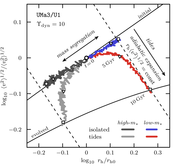
Figure 6: The effects of mass segregation on a stellar system are separable from tidal effects. The final ratio of half-light radii between the low-mass and high-mass populations is virtually unaffected by the adiabatic expansion of the stellar component in response to tides. Shown are the evolution of half-light radius and velocity dispersion of the UMa3/U1 model, in isolation (blue and dark grey curves for the low- and high-mass populations, respectively), and for the case of a tidal field that slowly lowers the dark matter mass enclosed within the stellar component (red and light grey curves). Circles, triangles and squares mark simulation times of $0\,\mathrm{Gyr}$, $5\,\mathrm{Gyr}$ and $10\,\mathrm{Gyr}$. Black solid curves illustrate the potential landscape at the beginning of the simulation (top curve, “initial”) and after $10\,\mathrm{Gyr}$ (bottom curve, “evolved”) for the simulation with tides, see text for details.

5 Conclusions

Summary. In the present work, we show that effects of collisional relaxation may play a substantial role for the dynamical evolution of a stellar component even in dark matter-dominated system. This is of particular relevance for old stellar systems with short crossing times, where small collisional perturbations can accumulate over the course of several gigayears. We show that for such systems, collisional relaxation drives stellar mass segregation and the dynamical formation of binaries even in presence of a gravitationally dominant smooth dark matter component. Our results hence call for caution when using stellar mass segregation as a litmus test for the absence of dark matter in ambiguous stellar clusters (Kim et al., 2015; Baumgardt et al., 2022; Simon et al., 2024; Zaremba et al., 2025) and tidal streams (Errani et al., 2022). Detailed modelling of the relaxation time scale and the Poisson noise floor is required to put constraints on the dark matter content of a stellar system through the observable signatures of mass segregation.

Caveats. Our models make various simplifying assumptions. Most crucially, the stellar populations are modelled as a two-component system of high- and low mass stars, both initially sharing the same half-light radius. The relaxation time of a stellar system sensitively depends on its stellar mass function and the abundance of high-mass stars. Our models do not include high-mass stellar remnants which may constitute a source of additional collisional perturbations which could amplify and speed up mass segregation. In that regard we believe our modelling choices to be conservative, putting a lower bound on the amount of mass segregation that is to be expected in presence of a smooth dark matter subhalo.

Furthermore, our models are tailored to describe systems that remain dark matter-dominated throughout their evolution, and neglect the dynamical effects of the stars on the dark matter distribution. The same fluctuating tidal field which drives stellar mass segregation is likely to affect the dark matter as well, particularly in systems that are initially or become baryon-dominated. A detailed study of this effect is computationally expensive and beyond the scope of the current paper.

Outlook. The models developed in this work are motivated by the recent discovery of ambiguous stellar systems at the interface of the dwarf galaxy- and globular cluster regimes, nevertheless they can also find application in understanding the dynamical processes in the central regions of dwarf spheroidal- and ultra faint galaxies. While their half-mass relaxation times may exceed the age of the universe, mass segregation plausibly still plays a role in their centres, where dynamical time scales and stellar densities are similar those of the systems studied here. In addition to the effects of dynamical friction by the dark matter component, stellar mass segregation may further enhance the clustering of massive stars and their remnants in the centres of dwarf galaxies, plausibly playing a role in setting their merger rates and a potential accompanying gravitational wave signal. This in turn would facilitate the formation of massive black holes in the centres of dark matter-dominated dwarf galaxies. A quantitative analysis of this effect requires a detailed modelling of the stellar mass function beyond the two-component setup used in the present work, as well as a detailed modelling of the dynamical response of the dark matter cusp, which we defer to subsequent study.

References

References

- Aarseth (1999) Aarseth, S. J. 1999, PASP, 111, 1333, doi: 10.1086/316455
- Amorisco & Evans (2012) Amorisco, N. C., & Evans, N. W. 2012, MNRAS, 419, 184, doi: 10.1111/j.1365-2966.2011.19684.x
- Barnes & Hut (1986) Barnes, J., & Hut, P. 1986, Nature, 324, 446, doi: 10.1038/324446a0
- Bastian & Lardo (2018) Bastian, N., & Lardo, C. 2018, ARA&A, 56, 83, doi: 10.1146/annurev-astro-081817-051839
- Baumgardt et al. (2022) Baumgardt, H., Faller, J., Meinhold, N., McGovern-Greco, C., & Hilker, M. 2022, MNRAS, 510, 3531, doi: 10.1093/mnras/stab3629
- Bovy (2015) Bovy, J. 2015, ApJS, 216, 29, doi: 10.1088/0067-0049/216/2/29
- Bruce et al. (2023) Bruce, J., Li, T. S., Pace, A. B., et al. 2023, ApJ, 950, 167, doi: 10.3847/1538-4357/acc943
- Buttry et al. (2022) Buttry, R., Pace, A. B., Koposov, S. E., et al. 2022, MNRAS, 514, 1706, doi: 10.1093/mnras/stac1441
- Cerny et al. (2023a) Cerny, W., Martínez-Vázquez, C. E., Drlica-Wagner, A., et al. 2023a, ApJ, 953, 1, doi: 10.3847/1538-4357/acdd78
- Cerny et al. (2023b) Cerny, W., Simon, J. D., Li, T. S., et al. 2023b, ApJ, 942, 111, doi: 10.3847/1538-4357/aca1c3
- Chabrier (2003) Chabrier, G. 2003, PASP, 115, 763, doi: 10.1086/376392
- Conn et al. (2018) Conn, B. C., Jerjen, H., Kim, D., & Schirmer, M. 2018, ApJ, 852, 68, doi: 10.3847/1538-4357/aa9eda
- Crnogorčević & Linden (2024) Crnogorčević, M., & Linden, T. 2024, Phys. Rev. D, 109, 083018, doi: 10.1103/PhysRevD.109.083018
- Devlin et al. (2025) Devlin, S., Baumgardt, H., & Sweet, S. M. 2025, MNRAS, 539, 2485, doi: 10.1093/mnras/staf572
- Errani et al. (2024a) Errani, R., Ibata, R., Navarro, J. F., Peñarrubia, J., & Walker, M. G. 2024a, ApJ, 968, 89, doi: 10.3847/1538-4357/ad402d
- Errani & Navarro (2021) Errani, R., & Navarro, J. F. 2021, MNRAS, 505, 18, doi: 10.1093/mnras/stab1215
- Errani et al. (2024b) Errani, R., Navarro, J. F., Smith, S. E. T., & McConnachie, A. W. 2024b, ApJ, 965, 20, doi: 10.3847/1538-4357/ad2267
- Errani & Peñarrubia (2020) Errani, R., & Peñarrubia, J. 2020, MNRAS, 491, 4591, doi: 10.1093/mnras/stz3349
- Errani et al. (2018) Errani, R., Peñarrubia, J., & Walker, M. G. 2018, MNRAS, 481, 5073, doi: 10.1093/mnras/sty2505
- Errani et al. (2025) Errani, R., Walker, M. G., Rozier, S., Peñarrubia, J., & Navarro, J. F. 2025, arXiv e-prints, arXiv:2502.19475, doi: 10.48550/arXiv.2502.19475
- Errani et al. (2022) Errani, R., Navarro, J. F., Ibata, R., et al. 2022, MNRAS, 514, 3532, doi: 10.1093/mnras/stac1516
- Fellhauer et al. (2000) Fellhauer, M., Kroupa, P., Baumgardt, H., et al. 2000, NA, 5, 305, doi: 10.1016/S1384-1076(00)00032-4
- Graham & Ramani (2024) Graham, P. W., & Ramani, H. 2024, Phys. Rev. D, 110, 075011, doi: 10.1103/PhysRevD.110.075011
- Gratton et al. (2012) Gratton, R. G., Carretta, E., & Bragaglia, A. 2012, A&A Rev., 20, 50, doi: 10.1007/s00159-012-0050-3
- Hernquist (1990) Hernquist, L. 1990, ApJ, 356, 359, doi: 10.1086/168845
- Iwasawa et al. (2016) Iwasawa, M., Tanikawa, A., Hosono, N., et al. 2016, PASJ, 68, 54, doi: 10.1093/pasj/psw053
- Ji et al. (2019) Ji, A. P., Simon, J. D., Frebel, A., Venn, K. A., & Hansen, T. T. 2019, ApJ, 870, 83, doi: 10.3847/1538-4357/aaf3bb
- Kim et al. (2015) Kim, D., Jerjen, H., Milone, A. P., Mackey, D., & Da Costa, G. S. 2015, ApJ, 803, 63, doi: 10.1088/0004-637X/803/2/63
- Kirby et al. (2017) Kirby, E. N., Cohen, J. G., Simon, J. D., et al. 2017, ApJ, 838, 83, doi: 10.3847/1538-4357/aa6570
- Longeard et al. (2018) Longeard, N., Martin, N., Starkenburg, E., et al. 2018, MNRAS, 480, 2609, doi: 10.1093/mnras/sty1986
- Martin et al. (2016a) Martin, N. F., Geha, M., Ibata, R. A., et al. 2016a, MNRAS, 458, L59, doi: 10.1093/mnrasl/slw013
- Martin et al. (2016b) Martin, N. F., Ibata, R. A., Collins, M. L. M., et al. 2016b, ApJ, 818, 40, doi: 10.3847/0004-637X/818/1/40
- Martin et al. (2022) Martin, N. F., Venn, K. A., Aguado, D. S., et al. 2022, Nature, 601, 45, doi: 10.1038/s41586-021-04162-2
- Mateo (1998) Mateo, M. L. 1998, ARA&A, 36, 435, doi: 10.1146/annurev.astro.36.1.435
- Mau et al. (2020) Mau, S., Cerny, W., Pace, A. B., et al. 2020, ApJ, 890, 136, doi: 10.3847/1538-4357/ab6c67
- McConnachie (2012) McConnachie, A. W. 2012, AJ, 144, 4, doi: 10.1088/0004-6256/144/1/4
- McConnachie & Côté (2010) McConnachie, A. W., & Côté, P. 2010, ApJ, 722, L209, doi: 10.1088/2041-8205/722/2/L209
- Namekata et al. (2018) Namekata, D., Iwasawa, M., Nitadori, K., et al. 2018, PASJ, 70, 70, doi: 10.1093/pasj/psy062
- Navarro et al. (1996) Navarro, J. F., Frenk, C. S., & White, S. D. M. 1996, ApJ, 462, 563, doi: 10.1086/177173
- Navarro et al. (1997) Navarro, J. F., Frenk, C. S., & White, S. D. M. 1997, ApJ, 490, 493, doi: 10.1086/304888
- Peñarrubia (2019) Peñarrubia, J. 2019, MNRAS, 490, 1044, doi: 10.1093/mnras/stz2648
- Peñarrubia (2021) —. 2021, MNRAS, 501, 3670, doi: 10.1093/mnras/staa3700
- Peñarrubia (2023) —. 2023, MNRAS, 519, 1955, doi: 10.1093/mnras/stac3642
- Peñarrubia et al. (2010) Peñarrubia, J., Benson, A. J., Walker, M. G., et al. 2010, MNRAS, 406, 1290, doi: 10.1111/j.1365-2966.2010.16762.x
- Safarzadeh & Spergel (2020) Safarzadeh, M., & Spergel, D. N. 2020, ApJ, 893, 21, doi: 10.3847/1538-4357/ab7db2
- Simon et al. (2024) Simon, J. D., Li, T. S., Ji, A. P., et al. 2024, ApJ, 976, 256, doi: 10.3847/1538-4357/ad85dd
- Smith et al. (2024) Smith, S. E. T., Cerny, W., Hayes, C. R., et al. 2024, ApJ, 961, 92, doi: 10.3847/1538-4357/ad0d9f
- Spitzer (1987) Spitzer, L. 1987, Dynamical evolution of globular clusters
- Springel (2005) Springel, V. 2005, MNRAS, 364, 1105, doi: 10.1111/j.1365-2966.2005.09655.x
- Stücker et al. (2023) Stücker, J., Ogiya, G., Angulo, R. E., Aguirre-Santaella, A., & Sánchez-Conde, M. A. 2023, MNRAS, 521, 4432, doi: 10.1093/mnras/stad844
- van den Bosch et al. (2018) van den Bosch, F. C., Ogiya, G., Hahn, O., & Burkert, A. 2018, MNRAS, 474, 3043, doi: 10.1093/mnras/stx2956
- Venn et al. (2004) Venn, K. A., Irwin, M., Shetrone, M. D., et al. 2004, AJ, 128, 1177, doi: 10.1086/422734
- Walker et al. (2007) Walker, M. G., Mateo, M., Olszewski, E. W., et al. 2007, ApJ, 667, L53, doi: 10.1086/521998
- Wang et al. (2020a) Wang, L., Iwasawa, M., Nitadori, K., & Makino, J. 2020a, MNRAS, 497, 536, doi: 10.1093/mnras/staa1915
- Wang et al. (2020b) Wang, L., Nitadori, K., & Makino, J. 2020b, MNRAS, 493, 3398, doi: 10.1093/mnras/staa480
- White & Rees (1978) White, S. D. M., & Rees, M. J. 1978, MNRAS, 183, 341, doi: 10.1093/mnras/183.3.341
- Yuan et al. (2022) Yuan, Z., Martin, N. F., Ibata, R. A., et al. 2022, MNRAS, 514, 1664, doi: 10.1093/mnras/stac1399
- Zaremba et al. (2025) Zaremba, D., Venn, K., Hayes, C. R., et al. 2025, arXiv e-prints, arXiv:2503.05927, doi: 10.48550/arXiv.2503.05927
- Zhang & Amaro Seoane (2025) Zhang, F., & Amaro Seoane, P. 2025, ApJ, 980, 210, doi: 10.3847/1538-4357/adaa7a