From chords to dynamical wormholes with matter:
Towards a bulk double-scaled (SYK) algebra

Abstract

We formulate a bulk description of the double-scaled algebra of the DSSYK model Lin:2022rbf . Based on the Hartle-Hawking (HH) state with matter chords, we derive several properties of the DSSYK model with heavy or light matter chords, without making assumptions about the specific dual theory, including its semiclassical thermodynamics, correlation functions, and Krylov complexity. These quantities are found from the saddle points of the DSSYK path integral preparing the HH state. We also construct a Lanczos algorithm that simultaneously evaluates Krylov state and operator complexity in the two-sided Hamiltonian system including finite temperature effects. In the semiclassical limit, both measures are encoded in the saddle points of the path integral. They have a bulk interpretation in terms of minimal geodesic lengths in AdS₂ space with backreaction due to a shockwave. Different saddle points correspond to geodesic distances with different asymptotic boundary time evolution, and they display different scrambling properties. This allows us to quantize the bulk dual theory of the DSSYK model, which we find is sine dilaton gravity, assuming the Schrödinger equation and momentum shift symmetry. At last, we deduce the boundary/bulk dictionary of the double-scaled algebra.

1 Introduction

Motivation

Bulk matter fields/ dual boundary operators are responsible for rich dynamics in holographic dictionary. These are indispensable components to build interesting models that resemble some aspects of our universe. It is thus important to thoroughly study dynamical observables that encode how bulk matter fields backreact in the geometry. A promising testing ground to carry out a comprehensive study involving bulk matter from a boundary perspective is the double-scaled SYK (DSSYK) model Berkooz:2018qkz ; Berkooz:2018jqr . It has a remarkable balance between interesting features for quantum gravity, and some degree of simpleness of working in lower dimensions. The model is UV finite and the rules for general amplitudes within the model have been derived by Berkooz:2018jqr . Meanwhile, at very low energies, the DSSYK model can describe the Schwarzian mode (as well as certain deformations Berkooz:2024ifu ) of Jackiw-Teitelboim (JT) JACKIW1985343 ; TEITELBOIM198341 gravity; and de-Sitter JT gravity in a similar but opposite regime Okuyama:2025hsd . There are several approaches to holography in this model, including dS₃ space in the s-wave reduction Susskind:2021esx ; Susskind:2022bia ; Lin:2022nss ; Rahman:2022jsf ; Rahman:2023pgt ; Rahman:2024iiu ; Rahman:2024vyg ; Narovlansky:2023lfz ; Verlinde:2024znh ; HVtalks ; Verlinde:2024zrh ; Gaiotto:2024kze ; Tietto:2025oxn ; Milekhin:2023bjv ; Yuan:2024utc ; Aguilar-Gutierrez:2024nau (which depend on gauge conditions, the physical operators and energy sectors of the DSSYK spectrum) and sine dilaton gravity Blommaert:2023opb ; Blommaert:2024whf ; Blommaert:2024ydx ; Blommaert:2025avl . It is expected in all of them that the so-called matter chords in this model play the role of matter fields in the bulk dual. However, while there has been great progress in deriving the holographic dictionary of the DSSYK model without matter in these mentioned approaches, there is currently no study on how the double-scaled algebra Lin:2022rbf enters in their proposals.

The double-scaled algebra

As originally proposed in Lin:2022rbf , and later developed in Xu:2024hoc , the double-scaled algebra is a type II₁ Von Neumann algebra of the DSSYK model defined by strings of operators (i.e. a finite linear span involving a polynomial of the generators Xu:2024hoc ) of the form

$$\expectationvalue{\hat{H}_{L/R},\leavevmode\nobreak\ \hat{\mathcal{O}}^{L/R}_{\Delta}}^{\prime\prime}\leavevmode\nobreak\ ,$$ (1)

where $\expectationvalue{\cdot,\cdot}$ indicates an algebra of bounded operators, which in this case includes (i) the two-sided DSSYK Hamiltonians $\hat{H}_{L/R}$ (16), and (ii) matter chord operators $\hat{\mathcal{O}}^{L/R}_{\Delta}$ (149) with a conformal weight $\Delta$, and ^′′ indicates closure of the algebra under the double commutant.

In order to identify the dual bulk theory of the DSSYK model, it is crucial to formulate the holographic dictionary for the boundary operators (1) in terms of the bulk-to-boundary map Lin:2022rbf . For this reason, we need to deduce what quantum observables encode the dynamics of the dual bulk geometry with matter fields. For instance, as noticed in Berkooz:2022fso , two-sided two-point functions are useful dynamical probes from the boundary side that encode length in the bulk with matter fields. However, we want to emphasize on its connection with holographic complexity (treated from a boundary perspective) to derive the holographic dictionary.

Krylov complexity

We will work with a boundary measure of bulk geodesics lengths, Krylov complexity Balasubramanian:2022tpr ; Parker:2018yvk (which we review in App. C.2). It has been shown that a wormhole (i.e. an Einstein-Rosen bridge) geodesic distance in an AdS₂ black hole background matches with Krylov complexity for the thermofield double (TFD) state at infinite temperature of the DSSYK model Rabinovici:2023yex . The authors make a connection of their results with JT gravity, which is recovered in the very low temperature regime instead. This is an interesting observation given that JT gravity corresponds to very low-energy regime (corresponding to very low temperatures in the microcanonical ensemble) instead. How can the infinite temperature TFD of the DSSYK model describe a geodesic length in JT gravity? Given that the triple-scaling limit involves a shift $\ell\rightarrow\ell+2\log\lambda$, where $\ell\sim\mathcal{O}(1)$ while $\lambda\rightarrow 0$, the renormalized bulk length in the JT gravity (i.e. subtracting $2\log\lambda$) should also be reproduced by the bulk theory dual to the DSSYK (i.e. without a triple-scaling limit). In the sine-dilaton gravity, Blommaert:2023opb ; Blommaert:2024whf ; Blommaert:2024ydx ; Blommaert:2025avl ; Bossi:2024ffa , there is an effective AdS₂ geometry, valid even at infinite temperatures. Krylov complexity is a natural measure of distance in the dual effective geometry, as observed in Heller:2024ldz .

There have been several other relevant developments. The properties of the DSSYK model with particle insertions have been better understood Lin:2022rbf ; Lin:2023trc ; Xu:2024hoc ; Xu:2024gfm . Krylov complexity for states and operators in the DSSYK model with and without one-particle insertions has been investigated in Xu:2024gfm ; Ambrosini:2024sre . Xu:2024gfm derived several dynamical observables relating the zero and one-particle chord space of the DSSYK model. Shortly after, an explicit Krylov basis and Lanczos coefficients for one-particle chord states was derived by Ambrosini:2024sre . The authors showed that the total chord number with a one chord matter operator insertion is indeed the Krylov complexity operator in the semiclassical limit. In this limit chords get very dense and they might provide an emergent bulk geometry Berkooz:2022fso . This fact allowed them to evaluate the Krylov complexity for the matter chord operator, and for a TFD state with a matter chord insertion. Soon afterwards, it was reported in Heller:2024ldz that, in the case without matter, one could interpret the spread complexity as a wormhole distance in an (effective) AdS₂ spacetime prepared in the Hartle-Hawking (HH) state at finite temperature. It has also realized and stressed by Heller:2024ldz that spread complexity is a natural candidate dual to the complexity equals volume (CV) proposal Susskind:2014rva ; Stanford:2014jda (at least in this model) if the switchback effect is also satisfied. While it is known that Krylov complexity for states and operators for particular states of the DSSYK model experience late-time linear growth Rabinovici:2023yex ; Ambrosini:2024sre ; Xu:2024gfm , it remains to be seen if the switchback effect can also be realized by Krylov complexity. Therefore, Krylov complexity might be promoted to a full-fledged entry in the holographic dictionary of the DSSYK model. We will address this in an upcoming work AX .

Other relevant developments in Krylov space methods for the DSSYK model can be found in Bhattacharjee:2022ave ; Aguilar-Gutierrez:2024nau ; Anegawa:2024yia ; Nandy:2024zcd ; Balasubramanian:2024lqk ; Miyaji:2025ucp .

To summarize, we are motivated to compare the following observables to identify the holographic dual of the DSSYK and its holographic dictionary:

• On the boundary side: There is no unique definition of quantum complexity that should be used. Krylov complexity is a valid candidate. Since it is defined in a gauge invariant matter, it should have a geometric description in the holographic dictionary.

• On the bulk side: Previous works indicate that geodesic lengths connecting the asymptotic boundaries in an AdS black hole geometry can be matched to Krylov complexity Rabinovici:2023yex ; Xu:2024gfm ; Heller:2024ldz . We will show that the boundary-to-bulk map of the DSSYK Lin:2022rbf is manifested in terms of Krylov complexity.

Double-scaled PETS

To investigate the holographic dictionary, we need to prepare states with operator insertions of the double-scaled algebra Lin:2022rbf on the unique tracial state Xu:2024hoc . This results in a two-sided Hamiltonian system, with a temperature associated to each side due due to modification of the would-be TFD state. In other words, we construct a double-scaled version of the partially entangled thermal states (PETS), originally defined for the finite N SYK model in Goel:2018ubv . The relative temperature difference corresponds to the angle of insertion of the operator along the thermal circle in the chord diagram. These types of states in the one-particle space have appeared in a recent study Xu:2024gfm . Our work instead explores how the light or heavy chord operators can be used to derive explicit observables that encode the dual minimal length geodesics.

Our analysis of the properties of the two-sided HH PETS (shown explicitly in (7)) is also motivated by three factors.

• The two-sided HH state contains information about the conformal dimensions and the evolution of matter chord operators acting on the unique tracial state of the DSSYK model. This makes it a natural reference state to study dynamical observables at finite temperature.

• The classical phase space variables in the DSSYK model in the HH state is closely related with geodesic lengths in the semiclassical limit. The phase space analysis of the DSSYK model has allowed much progress in the bulk dual proposals Narovlansky:2023lfz ; Blommaert:2024ydx ; Blommaert:2024whf .

1.1 Main questions and findings

In order to properly understand the role of matter fields in the dual theory of the DSSYK model, our main question is

What is the bulk dual of the double-scaled algebra?

By deducing the holographic dictionary (see Tab. 1), and performing the canonical quantization of the bulk dual theory, we formulate (1) in the terms of bulk operators

$$\expectationvalue{\hat{H}^{(\rm ADM)}_{L/R},\leavevmode\nobreak\ \hat{\xi}^{L/R}}^{\prime\prime}\leavevmode\nobreak\ ,$$ (2)

where $\hat{H}^{(\rm ADM)}_{L/R}$ are ADM Hamiltonians, $\hat{\xi}^{L/R}$ are quantized minimally coupled scalar fields in a two-sided AdS₂ effective background (82). The bulk theory that reproduces these results has constraints. Namely, as observed in the original works Blommaert:2024whf ; Blommaert:2024ydx (without matter), by demanding that the bulk states obey a Schrödinger equation and a momentum shift symmetry, one can reproduce the two-sided DSSYK Hamiltonian with matter. These need to be implemented through constraint quantization. This leads to the correspondence between the bulk and the DSSYK model with matter chords beyond the semiclassical limit, including their algebras of observables. However, we clarify that using other constraints in the chord Hilbert space results in other bulk duals A .

Krylov complexity as a probe of bulk/boundary dynamics

As highlighted in Sec. 1, there is not a sufficient understanding about the Krylov complexity with matter chords in the literature, especially when considering more than one-particle chords, in a finite temperature ensemble, and beyond the triple-scaling limit. For this reason, we will deduce a Lanczos algorithm for two-sided Hamiltonians that improves on these aspects. The reference state. It then natural to ask:

What properties of double-scaled matter operators are encoded in the evolution of Krylov complexity for a the two-sided HH state? What is its bulk interpretation? How does it compare with holographic complexity conjectures in other settings?

The conformal dimensions and the operators insertion times are encoded in the Krylov operator or spread complexity of the two-sided HH state. By matching the saddle point solutions/Krylov complexity to a minimal length geodesic in an AdS₂ black hole with massive particles or shockwave insertions. The holographic dictionary then follows. The Krylov operator and spread complexity correspond to geodesic lengths with different boundary time evolution. Krylov operator complexity displays several features (such as scrambling of information, hyperfast growth, and it obeys certain bounds) that have appeared in other contexts in the literature, e.g. Susskind:2021esx ; Milekhin:2024vbb ; Susskind:2014rva .

Lastly, we also connect our results to recent a proposal relating the proper momentum of a probe particle in asymptotically AdS geometries with the time derivative of Krylov complexity Caputa:2024sux ; Caputa:2025dep . We show that the radial proper momentum corresponds to the growth of Krylov operator complexity. The holographic dictionary is consistent with our findings in Tab. 1. The boundary answer then indicates a bulk prediction relating the wormhole distance (encoded in Krylov operator complexity) and the radial proper momentum of a probe particle.

Path integral, Krylov space and chord diagram approaches

The path integral approach is useful to prepare the two-sided HH state. However, the exact way to make the path integral preparation of state is not clearly addressed for two-sided Hamiltonian systems, where one has more freedom in how to generate the Hamiltonian evolution. For this reason,

How should one systematize the procedure to uniquely determine the path integral that prepares a given state in the two-sided Hamiltonian system with matter?

We will use the Heisenberg picture to formalize this point above, and derive what conditions one needs to impose in the saddle point solution preparing the HH state. The saddle point solution for the total chord number is equivalent to the semiclassical Krylov complexity of the HH state. As for the chord diagram perspective, it has been previously realized that two-sided two-point functions in the DSSYK model (corresponding to crossed four-point functions) also reproduce bulk geodesics in shockwave AdS₂ black hole geometries Berkooz:2022fso . However these developments are also limited to the triple scaling limit, and have a different formulation where there is no clear connection with the path integral nor Krylov complexity results in the more recent literature.

Do these different approaches, namely Krylov complexity, path integral and chord diagrams, encode equivalent information about the bulk dual geometry once we incorporate matter?

We find that all these methods encode a minimal length geodesic in the bulk. This is not unexpected since the path integral and Krylov complexity approaches relay on chord diagram Hamiltonian Lin:2022rbf . However, the way that this information is encoded in each measure is in principle different. While all these approaches reproduce the same minimal geodesic length in semiclassical limit; the relationship between these methods is more involved away from this regime. For instance, as previously reported in Ambrosini:2024sre , and as we also show under more general considerations in Sec. 3 and App. H, the total chord number is equivalent to Krylov complexity operator only in the $\lambda\rightarrow 0$ limit. Meanwhile, as reported in Xu:2024gfm , in general the Krylov basis is a function of the total chord number, even away from the semiclassical limit. Nevertheless, each method offers different technical and conceptual advantages.

1.2 Summary

A table summarizing the holographic dictionary of the DSSYK with matter chords and a compatible bulk dual theory (sine dilaton gravity Blommaert:2023opb ; Blommaert:2024whf ; Blommaert:2024ydx ; Blommaert:2025avl with matter) is displayed in Table 1.

Boundary (DSSYK)	Bulk (AdS2 black hole)
Two-sided HH state with an operator insertion, $\ket{\Psi_{\Delta}}$ (7)	Black hole in the HH state with a particle insertion (82)
Hamiltonian time $t_{L/R}$	Asymptotic boundary time $u_{L/R}$
Krylov complexity with a relative	Minimal geodesic distance between
two-sided time evolution $\eta=t_{R}/t_{L}$,	asymptotic boundaries,
$\lambda\leavevmode\nobreak\ \mathcal{C}^{(\eta)}(t)$ (57)	$L_{\rm AdS}(u_{L}=\eta u,u_{R}=u)$ (90)
Conformal dimension $\Delta$	Mass of minimally coupled scalar $m_{\xi}$
Inverse fake temperature $J\beta_{\rm fake}^{L/R}=\sin\theta_{L/R}$	Inverse bulk temperature $\beta{\rm AdS}$
Case 1: massive scalar
$4\pi\frac{\sin^{2}\theta+\eta q^{\Delta}\mathrm{e}^{-\ell_{*}(\theta)}}{\sin^{2}\theta-\eta q^{\Delta}\mathrm{e}^{-\ell_{*}(\theta)}}$	Backreaction parameter $\frac{8\pi G_{N}L_{b}}{\Phi_{b}}m_{\xi}$
$\ell_{*}(\theta)+2\log\frac{\sin^{2}\theta-\eta q^{\Delta}\mathrm{e}^{-\ell_{*}(\theta)}}{2\sin^{2}\theta}$	Regulator length $L_{\rm reg}-\frac{8G_{N}m_{\xi}L_{b}}{\Phi_{b}}$
Case 2: single shockwave
Shift parameter $\alpha_{\rm sw}$	$\frac{1}{4}\quantity(1-\frac{q^{\Delta_{\rm S}}\mathrm{e}^{-\ell_{*}}}{\sin^{2}\theta})$
Regularization length $L_{\rm reg}$	$\ell_{*}(\theta)$

Table 1: Holographic dictionary obtained from the match of Krylov complexity in the DSSYK with matter chords and wormhole lengths in an AdS₂ black hole geometry. $\ell_{*}(\theta)$ is the initial total chord number (31); $L_{b}/\Phi_{b}$ a regularized ratio between bulk parameters. App A provides a detailed overview of the notation implemented in the table.

In this work, we first introduce the concept of a double-scaled PETS as a natural generalization of the HH state in the chord Hilbert space DSSYK model with arbitrarily many particles. This provides valuable information for defining dynamical observables in finite temperature ensembles. We construct the partition function, and thermal two-point functions by taking expectation values with respect to the two-sided HH state (which are evaluated using chord diagram amplitudes in the App. D, E). We will then derive the path integral that prepares the two-sided HH state (deriving the equations of motion (EOM) and the initial conditions for the canonical variables from the Heisenberg picture). We then solve for the saddle points of the path integral, and the evolution of the total chord number in the HH state. From this calculation, one can easily deduce thermal two-point correlation functions for heavy or light operators in the semiclassical limit.

We will then define a double-scaled version of precursor operators (which originate from circuit complexity and the CV conjecture Susskind:2014rva ). This will allow us to study the saddle point solutions in a particular limit where the expectation value of the total chord number evolves in the same way as minimal length shockwave geodesics Shenker:2013pqa .

Later, we construct the Krylov basis of the DSSYK model with the two-sided HH state as reference in the Lanczos algorithm for two-sided Hamiltonians. The key advantage of this formulation is that we can evaluate both Krylov operator or spread complexity at once and including finite temperatures. We show that the total chord number is the Krylov complexity operator in the semiclassical limit (using similar arguments as Ambrosini:2024sre , while allowing for finite temperature effects). This also implies that the thermal two-point function (58) takes the role of the generating function of Krylov complexity (and higher moments) in the semiclassical limit. Furthermore, both types of Krylov complexity correspond to geodesic lengths in the bulk with different relative time orientation due to the two-sided Hamiltonian evolution. Our results reproduce those in the literature as special cases. (i) Taking an infinite temperature limit Ambrosini:2024sre , and (ii) considering a vanishing conformal weight of the matter operator Heller:2024ldz .

Importantly, the Krylov operator complexity displays a transition from exponential to linear growth. The results show that the scrambling time in Krylov operator complexity corresponds to the time scale of decay in the corresponding out-of-time-ordered correlator (OTOC). The latter is a different and more commonly used definition of scrambling time Xu:2022vko . We find that it does not depend on the system size, which is a property we will refer to as hyperfast growth Anegawa:2024yia , in contrast with the bound on the fastest information scrambling in Sekino:2008he (which is proportional to an exponential of the system’s entropy). The OTOC obeys general bounds on fermionic systems Milekhin:2024vbb , and its exponent satisfies the chaos bound Maldacena:2015waa .

Our results on thermal two-sided two-point functions and Krylov complexity, and more details on the holographic dictionary are summarized in App. B.

Later on, we elaborate on the bulk description of our results. We first study JT and sine dilaton gravity with a minimally coupled scalar field in an (effective) AdS₂ black hole background. We show that a wormhole geodesic distance matches with Krylov operator complexity of the two-sided HH state when the backreaction in the bulk is perturbatively small. Then, we take a non-perturbative approach using shockwave backreaction. We match our results on classical phase space from the path integral with precursor operator insertions to geodesic lengths in an AdS₂ shockwave geometry Shenker:2013pqa . From our results, we carry on the constraint quantization of the bulk theory (sine-dilaton gravity) and derive a holographic description of the double-scaled algebra.

Thus, since Krylov complexity measures a wormhole in the bulk (i.e. one of the classical phase space variables in JT and sine dilaton gravity), this is a crucial element in the holographic dictionary of the DSSYK model. We hope this reveals useful lessons in more generic systems, even if Krylov is not always an appropriate measure of quantum chaos. We also stress that we do not assume a priori a correspondence between sine dilaton gravity with the DSSYK model or other bulk theory, we simply show that our boundary side results are compatible with sine dilaton gravity with matter. We later canonically quantize the bulk theory to show that it is indeed dual to the DSSYK model with one-particle, and to derive the dual double-scaled algebra.

Other technical results are included in the appendices. In particular, we derive the semiclassical thermodynamics of the system from the partition function in the microcanonical ensemble (e.g. the heat capacity, to determine thermal stability). We also evaluate two (or four)-point correlation functions from chord diagrams. This serves as a consistency check of our results from classical phase space methods. The evaluation involves a new R-matrix calculation in the DSSYK model (also seen as a 6-j symbol of $\mathcal{U}_{q}(\text{su}(1,1))$ Berkooz:2018jqr ; Blommaert:2023opb ; Belaey:2025ijg ) in the semiclassical limit. Some of the technical steps in the calculation follow similarly from evaluating OTOCs in JT gravity Mertens:2017mtv ; Lam:2018pvp ; Mertens:2022irh . However, while the phase space answer is valid for heavy and light particles, the chord diagram calculation uses an ansatz valid only for light operators. Due to this technical limitation we have not crossed verified the calculation for the heavy operator case from the chord diagram methods. Nevertheless, we find agreement in the expected regime of validity with out path integral results.

The reader interested in a quick overview of the main results may check App. B (complemented by a summary of the notation in App. A).

Plan of the manuscript

In Sec. 2, we define the two-sided HH state (7) in the one-particle chord space, we study the path integral preparing this state, and its saddle points. In Sec. 3 we derive Krylov operator and spread complexity in the irrep. one-particle chord space from a Lanczos algorithm for two-sided Hamiltonians with the two-sided, finite temperature HH state as reference state. We also discuss specifically about Krylov operator and spread complexity. In Sec. 4, we study bulk geodesics with backreaction, which we match to the Krylov operator and spread complexity to derive the holographic dictionary, perform the canonical quantization of the bulk theory, and formulate the double-scaled algebra in bulk terms. We also comment on the proper momentum of a point particle in an AdS₂ black hole. Sec. 5 concludes with a discussion and an outlook.

For the ease of reading, App. A includes a list of the notation (including acronyms) used in the manuscript. App. B is a list of the main outcomes from our study. To keep the presentation self-contained, App. C reviews useful results on (i) the DSSYK model (App. C.1), and Krylov complexity for states and operators (App. C.2). Meanwhile, App. D contains new results regarding the semiclassical thermodynamics in the two-sided HH state, including derived quantities in the microcanonical ensemble (temperature, entropy, and heat capacity). In App. E we calculate the thermal two-point correlation function in the particle chord space (an crossed four-point function in $\mathcal{H}^{L}_{0}\otimes\mathcal{H}_{0}^{R}$, which we illustrate in Fig. 2). Meanwhile, in App. G we analyze the properties of the semiclassical OTOC in (33). In App. F, we discuss a criterion to determine if states in $\mathcal{H}_{m}$ have a smooth geometries in the bulk dual theory Berkooz:2022fso . App. H contains technical details about the Lanczos coefficients and Krylov basis. At last, App. I shows how to decompose more general states in $\mathcal{H}_{m}$ into $\mathcal{H}_{0}$ and $\mathcal{H}_{1}$ irreps.

2 The Euclidean path integral of the DSSYK with matter chords

In this section, we explain how to prepare the two-sided HH state from the Euclidean path integral of the DSSYK, and we study its saddle point solutions.

Outline

In Sec. 2.1 we explain basic properties about the two-sided HH state, its partition function (discussed in detail in App. D), and how to simplify expressions with composite chord matter operators. In Sec. 2.2 we discuss the path integral that prepares the two-sided HH state. We first derive the Heisenberg equations for canonical operators in the two-sided theory, and the initial conditions for their expectation values. This allow us to determine the correct path integral for the two-sided HH state. The real part of the complexified time is related to the temperature of the system (in the microcanonical ensemble), and the imaginary part with real-time evolution. In Sec. 2.3 we study two-sided two point correlation functions using the classical phase space results in the path integral. In Sec. 2.4 we point out significant modifications in the state preparation by allowing for time dependence in the Schrödinger picture operators (known as precursors Susskind:2014rva ) which are inserted on the two-sided HH state.

2.1 Partially entangled thermal states from double-scaled operators

To set the stage, we first explain how to build states on the chord Hilbert space, $\hat{\mathcal{H}}_{m}$ ($m$ labels the total number of particle chords) where the algebra (1) closes. The Hilbert space $\mathcal{H}_{m}$ takes the form Lin:2022rbf

$$\mathcal{H}_{m}=\bigoplus_{n_{0},n_{1},\dots,n_{m}=0}^{\infty}\mathbb{C}\ket{\tilde{\Delta};n_{0},n_{1},\dots,n_{m}}\leavevmode\nobreak\ ,$$ (3)

where $\tilde{\Delta}=\quantity{\Delta_{1},\cdots,\Delta_{m}}$, represents a string of matter operator insertions

$$\hat{\mathcal{O}}_{\tilde{\Delta}}=\quantity{\hat{\mathcal{O}}_{\Delta_{1}},\dots,\leavevmode\nobreak\ \hat{\mathcal{O}}_{\Delta_{m}}}\leavevmode\nobreak\ ,\quad m\in\mathbb{Z}_{\geq 0}\leavevmode\nobreak\ ;$$ (4)

while $n_{0}$ is the number of DSSYK chords (called H-chords) to the left of all matter chords, $n_{1}$ the number between the first two particles; all the way up to the number of chords between all the $m$ particles. We review this in more detail in App. C.1. As shown in Xu:2024hoc , one can generate any element in the DSSYK Hilbert space $\mathcal{H}_{m}$ by acting with a string of bounded double-scaled operators in (1) with appropriate operator ordering on the unique tracial state $\ket{0}$.

The evolution of states in $\mathcal{H}_{m}$ is generated by the DSSYK two-sided Hamiltonian, which was originally constructed in Lin:2022rbf in terms of creation ($\hat{a}_{i}^{\dagger}$) and annihilation ($\hat{\alpha}_{i}$) operators as

$$\hat{H}_{L} =\frac{J}{\sqrt{\lambda}}\quantity(\hat{a}^{\dagger}_{0}+\sum_{i=0}^{m}\hat{\alpha}_{i}\quantity(\frac{1-q^{\hat{n}_{i}}}{1-q})q^{\hat{n}_{i}^{<}})\quad\text{where}\quad\hat{n}_{i}^{<}=\sum_{j=0}^{i-1}\quantity(\hat{n}_{j}+\Delta_{j+1})\leavevmode\nobreak\ ,$$ (5a)

$$\hat{H}_{R} =\frac{J}{\sqrt{\lambda}}\quantity(\hat{a}^{\dagger}_{m}+\sum_{i=0}^{m}\hat{\alpha}_{i}\quantity(\frac{1-q^{\hat{n}_{i}}}{1-q})q^{\hat{n}_{i}^{>}})\quad\text{where}\quad\hat{n}_{i}^{>}=\sum_{j={i+1}}^{m}\quantity(\hat{n}_{j}+\Delta_{j})\leavevmode\nobreak\ ,$$ (5b)

where $J$ is a coupling constant, and $q=\mathrm{e}^{-\lambda}\in[0,1]$ is a parameter of the model (reviewed in App. C.1). Note that the triple scaling limit of (5) has been previously studied in Lin:2022rbf ; Xu:2024hoc . The action of the operators in $\mathcal{H}_{m}$ is displayed in (153a, 153b). Note that $\hat{\alpha}_{0/m}$ and $\hat{a}^{\dagger}_{0/m}$ are not Hermitian conjugate operators of each other with respect to the inner product for in the $\ket{\Delta;n_{0},\dots,n_{m}}$ basis Lin:2022rbf ; Lin:2023trc ; Ambrosini:2024sre . The Hamiltonians (16) can be brought to the same form as the auxiliary Hamiltonian of the DSSYK model with matter chords, see (155).

Double scaled PETS

We will now introduce a double-scaled version of the PETS, which was originally defined for the SYK model in Goel:2018ubv (and further studied in Goel:2023svz ; Jian:2020qpp ). In our construction, we insert two or more matter chord operators $\hat{\mathcal{O}}_{\Delta_{i}}^{L/R}$ of the double-scaled algebra (1) (which we review inn App C.1) in the thermal circle of the DSSYK model. We allow for unequal temperatures between the different subregions of the circle, and a two-sided Hamiltonian ($\hat{H}_{L/R}$) evolution in complex time, $\tau\in\mathbb{C}$ (where the imaginary part corresponds to the real time and the real one to the temperature dependence). This takes the form:

$$\ket{\Psi^{L/R}_{\tilde{\Delta}}(\tau_{0},\dots,\tau_{m})}= \mathrm{e}^{-\hat{H}_{L/R}\tau_{0}}\hat{\mathcal{O}}^{L/R}_{\Delta_{1}}\mathrm{e}^{-\hat{H}_{L/R}\tau_{1}}\dots\mathrm{e}^{-\hat{H}_{L/R}\tau_{m-1}}\hat{\mathcal{O}}^{L/R}_{\Delta_{m}}\mathrm{e}^{-\hat{H}_{L/R}\tau_{m}}\ket{0}\leavevmode\nobreak\ .$$ (6)

For explicit computations, we will mostly be interested in the special case below.

The two-sided Hartle-Hawking (HH) state

We define a two-sided HH state in $\mathcal{H}_{m}$ as a PETS (6) where the operators are arranged in form

$$\ket{\Psi_{\tilde{\Delta}}(\tau_{L},\tau_{R})} =\mathrm{e}^{-\tau_{L}\hat{H}_{L}-\tau_{R}\hat{H}_{R}}\ket{\tilde{\Delta};0,\dots,0}$$ (7)

$$=\mathrm{e}^{-\tau_{L}\hat{H}_{L}}\hat{\mathcal{O}}_{\Delta_{1}}\hat{\mathcal{O}}_{\Delta_{2}}\cdots\hat{\mathcal{O}}_{\Delta_{m-1}}\hat{\mathcal{O}}_{\Delta_{m}}\mathrm{e}^{-\tau_{R}\hat{H}_{R}}\ket{0}\leavevmode\nobreak\ ,$$

where $\tau_{L/R}=\mathrm{i}t_{L/R}+\beta_{L/R}/2$. Here, the left and right-sided real time evolution is parametrized by $t_{L/R}$; while $\beta_{L/R}$ represents the left and right inverse temperatures in the thermal circle (see Fig. 5).

We stress that the two-sided HH state in (7) is a composite operator propagating between two points in the thermal circle of chord diagrams, as displayed in Fig. 1 (a).

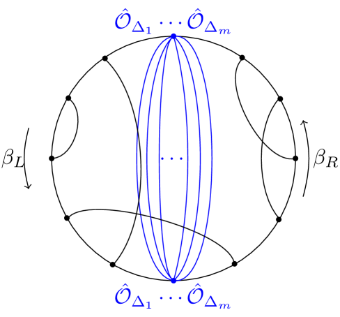
(a)

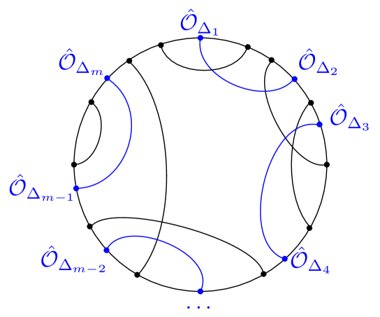
(b)

Figure 1: Chord diagram of (6) with (a) one composite operator insertion $\prod_{i=1}^{m}\hat{\mathcal{O}}_{\Delta_{i}}$ (blue); (b) Several non-composite operators $\hat{\mathcal{O}}_{\Delta_{i}}$. The thermal circle is divided into two portions with a periodicity associated to the left and right sectors $\beta_{L},\leavevmode\nobreak\ \beta_{R}$ with respect to the operator insertion. The black curves present Hamiltonian (H) chords.

This can be seen from the partition function:

$$Z_{\tilde{\Delta}}(\beta_{L},\beta_{R}) =\evaluated{\bra{\Psi_{\tilde{\Delta}}(\tau_{L},\tau_{R})}\ket{\Psi_{\tilde{\Delta}}(\tau_{L},\tau_{R})}}_{\tau_{L/R}=\frac{\beta_{L/R}}{2}}$$ (8)

$$=\bra{0}\hat{\mathcal{O}}^{L}_{\Delta_{1}}\cdots\hat{\mathcal{O}}^{L}_{\Delta_{m}}\mathrm{e}^{-\beta_{L}\hat{H}_{L}}\hat{\mathcal{O}}^{L}_{\Delta_{1}}\cdots\hat{\mathcal{O}}^{L}_{\Delta_{m}}\mathrm{e}^{-\beta_{R}\hat{H}_{L}}\ket{0}\leavevmode\nobreak\ ,$$

where we used the boost invariance: $(\hat{H}_{R}-\hat{H}_{L})\ket{0}=0$; and also $\hat{\mathcal{O}}_{\Delta}^{\dagger}=\hat{\mathcal{O}}_{\Delta}$.

We see from (8) that the total periodicity of the thermal circle must be $\beta_{L}+\beta_{R}$. Technical details on the evaluation are presented in App. D.

One may also study more observables whose expectation value is evaluated in the more general state (6) that has a relative phase (which is important for the switchback effect AX ). However, this introduces technical difficulties in our analysis, as we explain below. We provide more details on how to treat this case in App. I (see also AX ).

To make simplifications in the (7) we begin showing that

$$\prod_{i}\hat{\mathcal{O}}_{\Delta_{i}}\ket{0}=\hat{\mathcal{O}}_{\Delta_{\rm S}}\ket{0}\leavevmode\nobreak\ ,\quad\text{where}\quad\Delta_{\rm S}=\sum^{m}_{i=1}{\Delta_{i}}\leavevmode\nobreak\ .$$ (9)

This can be proved recursively using (82) in Lin:2023trc , which states that states in $\mathcal{H}_{2}$ can be decomposed into $\mathcal{H}_{1}$ irreducible representations (irreps):

$$\left|\Delta_{1},\Delta_{2};n_{L},n_{1},n_{R}\right\rangle=\sum_{m_{L}+m_{R}+l=n_{1}}\chi_{l,m_{L},m_{R}}\left|\Delta_{1}+\Delta_{2}+l;n_{L}+m_{L},n_{R}+m_{R}\right\rangle\leavevmode\nobreak\ ,$$ (10)

where $\chi_{k,m_{L},m_{R}}$ are Clebsch-Gordan coefficients. In particular, this implies

$$\ket{\Delta_{1},\Delta_{2};0,0,0}=\hat{\mathcal{O}}_{\Delta_{1}}\hat{\mathcal{O}}_{\Delta_{2}}\ket{0}=\hat{\mathcal{O}}_{\Delta_{1}+\Delta_{2}}\ket{0}=\ket{\Delta_{1}+\Delta_{2};0,0}\leavevmode\nobreak\ .$$ (11)

(9) follows straightforwardly. Then, $\prod_{i}\hat{\mathcal{O}}_{\Delta_{i}}$ acts as a composite operator in a generalized free field (GFF) theories in the large $N$ limit, where (9) also holds Duetsch:2002hc . This means that while (7) lives in $\mathcal{H}_{m}$, it can be reduced to a state in $\mathcal{H}_{1}$, which is a irreducible representation (irrep).

We also remark that

$$\mathrm{e}^{-\beta_{R}\hat{H}_{R}}\hat{\mathcal{O}}^{R}_{\Delta_{\rm S}}(t_{R})\mathrm{e}^{-\beta_{R}\hat{H}_{R}}\ket{0}=\mathrm{e}^{-\beta_{R}\hat{H}_{H}}\hat{\mathcal{O}}^{L}_{\Delta_{\rm S}}(t_{H})\mathrm{e}^{-\beta_{R}\hat{H}_{R}}\ket{0}=\ket{\Psi_{\tilde{\Delta}}(\tau_{R}^{*},\tau_{R})}\leavevmode\nobreak\ ,$$ (12)

so that we can choose to express everything purely in terms of $\hat{\mathcal{O}}^{L}_{\Delta_{\rm S}}$ and the associated Hamiltonians., which is similar to the “matching” property in Berkooz:2022fso . We will denote $\mathcal{O}_{\Delta}^{L}$ as $\mathcal{O}_{\Delta}$ from now on to simplify the notation. Thus, the two-sided correlator can be re-expressed as

$$\expectationvalue{\mathrm{e}^{-\beta_{L}\hat{H}_{L}}\hat{\mathcal{O}}_{\Delta_{\rm S}}(t_{L})\mathrm{e}^{-\beta_{L}\hat{H}_{L}}\hat{\mathcal{O}}_{\Delta_{w}}\mathrm{e}^{-\beta_{R}\hat{H}_{R}}\hat{\mathcal{O}}_{\Delta_{\rm S}}\mathrm{e}^{-\beta_{R}\hat{H}_{R}}\hat{\mathcal{O}}_{\Delta_{w}}(t_{R})}_{J,M}$$ (13)

$$=\bra{\Psi_{\tilde{\Delta}}(\tau_{L}^{*},\tau_{L})}q^{\Delta_{w}\hat{N}}\ket{\Psi_{\tilde{\Delta}}(\tau_{R}^{*},\tau_{R})}\leavevmode\nobreak\ .$$

From the bulk side, there is be an associated conformal factor problem in the Euclidean path integral, similar to what has been pointed out in higher dimensional settings (see e.g.Gibbons:1978ac ; Monteiro:2009tc ; Monteiro:2008wr ; Prestidge:1999uq ; Marolf:2021kjc ; Marolf:2022ybi ), which is dealt with by requiring finiteness of the dilaton Blommaert:2024whf . From the boundary side, this is equivalent to allowing the range of the energy parametrization, $\theta_{L/R}$, to extend beyond $[0,\pi]$, which leads to a thermodynamical instability in the saddle point solutions (see App. D). Well definiteness of the Euclidean path integral and thermal stability are also linked together in higher dimensional examples (e.g. Monteiro:2008wr ; Prestidge:1999uq ).

2.2 Classical phase space from the Euclidean path integral

In this subsection, we solve for the classical phase space of the DSSYK in the two-sided HH state from path integral methods. First, we will derive the canonical variables in the quantum Hamiltonian of the theory, and the Heisenberg equations that they must satisfy.

We now redefine the creation and annihilation operators in (5) to its canonical form by identifying the distance $\hat{\ell}_{i}$, and momenta $\hat{P}_{i}$ operators, in analogy with the $\mathcal{H}_{0}$ case Lin:2022rbf

$$\hat{a}_{i}^{\dagger}=\frac{\mathrm{e}^{-\mathrm{i}\hat{P}_{i}}}{\sqrt{1-q}}\leavevmode\nobreak\ ,\quad\hat{\alpha}_{i}=\sqrt{1-q}\leavevmode\nobreak\ \mathrm{e}^{\mathrm{i}\hat{P}_{i}}\leavevmode\nobreak\ ,\quad q^{\hat{n}_{i}}=\mathrm{e}^{-\hat{\ell}_{i}}\leavevmode\nobreak\ ,$$ (14)

and we will denote

$$\hat{\ell}\equiv\sum_{i}\hat{\ell}_{i}=\lambda\hat{N}\leavevmode\nobreak\ ,\quad\hat{N}\equiv\sum_{i}\hat{n}_{i}$$ (15)

which we denote as the total chord number (154).

We can now express (5) as

$$\hat{H}_{L}=\frac{J}{\sqrt{\lambda(1-q)}}\quantity(\mathrm{e}^{-\mathrm{i}\hat{P}_{0}}+\sum_{i=0}^{m}\mathrm{e}^{\mathrm{i}\hat{P}_{i}}(1-\mathrm{e}^{-\hat{\ell}_{i}})\mathrm{e}^{-\hat{\ell}_{i}^{<}})\leavevmode\nobreak\ ,$$ (16a)

$$\hat{H}_{R}=\frac{J}{\sqrt{\lambda(1-q)}}\quantity(\mathrm{e}^{-\mathrm{i}\hat{P}_{m}}+\sum_{i=0}^{m}\mathrm{e}^{\mathrm{i}\hat{P}_{i}}(1-\mathrm{e}^{-\hat{\ell}_{i}})\mathrm{e}^{-\hat{\ell}_{i}^{>}})\leavevmode\nobreak\ ,$$ (16b)

where we define

$$\hat{\ell}_{i}^{<}=\sum_{j=0}^{i-1}\quantity(\hat{\ell}_{j}+\lambda\Delta_{j+1})\leavevmode\nobreak\ ,\quad\hat{\ell}_{i}^{>}=\sum_{j={i+1}}^{m}\quantity(\hat{\ell}_{j}+\lambda\Delta_{j})\leavevmode\nobreak\ .$$ (17)

In the following, we first solve for the dynamics of the model in the Heisenberg picture, which will allow us to derive the path integral that describes the two-sided system (16).

Quantum dynamics

We want to specify the quantum dynamics of the canonical operators in this theory. It is convenient to change from the Schrödinger to Heisenberg picture, by defining the operators

$$\hat{\ell}(\tau_{L},\tau_{R}) \equiv\mathrm{e}^{-\tau_{L}\hat{H}_{L}-\tau_{R}^{*}\hat{H}_{R}}\hat{\ell}\mathrm{e}^{-\tau_{L}\hat{H}_{L}-\tau_{R}\hat{H}_{R}}\leavevmode\nobreak\ ,$$ (18)

$$\mathrm{e}^{-\mathrm{i}\hat{P}_{0/m}(\tau_{L},\tau_{R})} \equiv\mathrm{e}^{-\tau_{L}\hat{H}_{L}-\tau_{R}^{*}\hat{H}_{R}}\mathrm{e}^{-\mathrm{i}\hat{P}_{0/m}}\mathrm{e}^{-\tau_{L}\hat{H}_{L}-\tau_{R}\hat{H}_{R}}\leavevmode\nobreak\ .$$

Note that expectation values in both pictures agree with each other, i.e.

$$\bra{\tilde{\Delta};0,\dots,0}\hat{\ell}(\tau_{L},\tau_{R})\ket{\tilde{\Delta};0,\dots,0}=\bra{\Psi_{\tilde{\Delta}}(\tau_{L},\tau_{R})}\hat{\ell}\ket{\Psi_{\tilde{\Delta}}(\tau_{L},\tau_{R})}\leavevmode\nobreak\ ,$$ (19)

$$\bra{\tilde{\Delta};0,\dots,0}\mathrm{e}^{-\mathrm{i}\hat{P}_{0/m}(\tau_{L},\tau_{R})}\ket{\tilde{\Delta};0,\dots,0}=\bra{\Psi_{\tilde{\Delta}}(\tau_{L},\tau_{R})}\mathrm{e}^{-\mathrm{i}\hat{P}_{0/m}}\ket{\Psi_{\tilde{\Delta}}(\tau_{L},\tau_{R})}\leavevmode\nobreak\ ,$$

where the two-sided HH state is defined (7).

The Heisenberg EOM become

$$-\frac{\mathrm{i}}{\lambda}\partial_{t_{L/R}}\hat{\ell}(\tau_{L},\tau_{R}) =[\hat{H}_{L/R},\leavevmode\nobreak\ \hat{\ell}(\tau_{L},\tau_{R})]=\hat{H}_{L/R}-\frac{2J}{\sqrt{\lambda(1-q)}}\mathrm{e}^{-\mathrm{i}\hat{P}_{0/m}(\tau_{L},\tau_{R})}\leavevmode\nobreak\ ,$$ (20a)

$$-\mathrm{i}\partial_{t_{R/L}}\mathrm{e}^{-\mathrm{i}\hat{P}_{m/0}(\tau_{L},\tau_{R})} =[\hat{H}_{L/R},\leavevmode\nobreak\ \mathrm{e}^{-\mathrm{i}\hat{P}_{m/0}(\tau_{L},\tau_{R})}]=J\sqrt{\frac{1-q}{\lambda}}q^{\Delta_{\rm S}}\mathrm{e}^{-\hat{\ell}(\tau_{L},\tau_{R})}\leavevmode\nobreak\ ,$$ (20b)

$$-\mathrm{i}\partial_{t_{R/L}}\mathrm{e}^{-\mathrm{i}\hat{P}_{m/0}(\tau_{L},\tau_{R})} =[\hat{H}_{L/R},\leavevmode\nobreak\ \mathrm{e}^{-\mathrm{i}\hat{P}_{0/m}}]_{q}-(1-q)\mathrm{e}^{-\mathrm{i}\hat{P}_{0/m}}\hat{H}_{L/R}$$ (20c)

$$=J\sqrt{\frac{1-q}{\lambda}}\quantity(1+\mathrm{e}^{-2\mathrm{i}P_{0/m}(\tau_{L},\tau_{R})})-(1-q)\mathrm{e}^{-\mathrm{i}\hat{P}_{0/m}}\hat{H}_{L/R}\leavevmode\nobreak\ ,$$

where we used the commutation relations for $\hat{a}_{L/R}$ and $\hat{H}_{L/R}$ in Lin:2023trc (28) together with (14).

Combining (20a) and (20b) we get a Liouville-like equation of motion:

$$-\partial_{t_{L}}\partial_{t_{R}}\hat{\ell}(\tau_{L},\tau_{R})=[\hat{H}_{L},\leavevmode\nobreak\ [\hat{H}_{R},\leavevmode\nobreak\ \hat{\ell}]]=-2J^{2}q^{\Delta_{\rm S}}\mathrm{e}^{-\ell}\leavevmode\nobreak\ ,$$ (21)

which is a dynamical version of (30) in Lin:2023trc (theirs use Euclidean time $\partial_{L/R}\equiv\partial_{\tau_{L/R}}$ instead). Note (21) is consistent with the Ehrenfest theorem for Krylov complexity in (2.23) of Erdmenger:2023wjg when $\Delta=0$ so that $\hat{H}_{L}=\hat{H}_{R}$ (and $t_{L}=t_{R}$) where the Krylov complexity operator is quantum mechanically equal to the chord number operator (with the HH state as reference state).

Next, we can also specify the initial conditions for the operator valued expectation values in the two-sided HH state (19),

$$\bra{\tilde{\Delta};0,\dots,0}\hat{\ell}\quantity(\tfrac{\beta_{L}}{2},\tfrac{\beta_{R}}{2})\ket{\tilde{\Delta};0,\dots,0}=\ell_{*}\leavevmode\nobreak\ ,$$ (22a)

$$\begin{aligned} &\evaluated{\partial_{t_{L/R}}\bra{\tilde{\Delta};0,\dots,0}\hat{\ell}(\tau_{L},\tau_{R})\ket{\tilde{\Delta};0,\dots,0}}_{t_{L/R}=0}\\ &=\bra{\tilde{\Delta};0,\dots,0}\mathrm{e}^{-\beta_{L}\hat{H}_{L}-\beta_{R}\hat{H}_{R}}[\hat{H}_{L/R},\leavevmode\nobreak\ \hat{\ell}]\mathrm{e}^{-\beta_{L}\hat{H}_{L}-\beta_{R}\hat{H}_{R}}\ket{\tilde{\Delta};0,\dots,0}=0\leavevmode\nobreak\ ,\end{aligned}$$ (22b)

where we derived (LABEL:eq:initial_velocity) from the cyclic property of the tracial state $\ket{0}$ Xu:2024hoc . In our case, this means

$$\bra{0}\hat{H}_{L/R}\mathcal{O}_{\Delta}^{L/R}\dots\mathcal{O}_{\Delta}\ket{0}=\bra{0}\mathcal{O}_{\Delta}\dots\mathcal{O}_{\Delta}^{L/R}\hat{H}_{L/R}\ket{0}\leavevmode\nobreak\ .$$ (23)

One can easily see that this cancellation does not occur for $t\neq 0$. Meanwhile, $\ell_{*}$ in (22a) is just a constant determined by the temperatures. We will show that the specific value (31) can be determined in terms of the conserved energy spectrum of the system (28). For instance, one can see that in the infinite temperature limit $\beta_{L/R}\rightarrow 0$, then $\ell_{*}=0$ (because $\hat{N}\ket{\tilde{\Delta};0,\dots,0}=0$). However, we will work with arbitrary values of the two-sided temperatures.

Thus, the evolving PETS HH state (7) generates expectation values satisfying the EOM (20) and the initial conditions (22).

Hartle-Hawking saddle point

We will now study the Euclidean path integral of (16) that prepares the two-sided HH state (7). While the path integral is, strictly speaking, not necessary (one can evaluate the expectation values directly in the $\lambda\rightarrow 0$ limit), it is convenient as we can think on the solutions as saddle points.

Based on our analysis of the Heisenberg picture operators, we should use

$$\int\prod_{i=0}^{m}[\mathrm{d}\ell_{i}][\mathrm{d}P_{i}]\exp\quantity[\int\mathrm{d}\tau_{L}\mathrm{d}\tau_{R}\quantity(\frac{\mathrm{i}}{\lambda}\sum_{i=0}^{m}\quantity(P_{i}(\partial_{\tau_{L}}+\partial_{\tau_{R}})\ell_{i})+H_{L}+H_{R})]\leavevmode\nobreak\ ,$$ (24)

where the operators in the two-sided Hamiltonian (16) have been exchanged for field variables. The saddle points of the path integral (when $\lambda\rightarrow 0$) are

$$(\partial_{t_{L}}+\partial_{t_{R}})\ell_{i}=\derivative{(H_{L}+H_{R})}{P_{i}}\leavevmode\nobreak\ ,\qquad(\partial_{t_{L}}+\partial_{t_{R}})P_{i}=-\derivative{(H_{L}+H_{R})}{\ell_{i}}\leavevmode\nobreak\ ,$$ (25)

where we have used $\tau_{L/R}=\frac{\beta_{L/R}}{2}+\mathrm{i}t_{L/R}$, with $\beta_{L/R}$ is a constant in time. We want to study the saddle points describing the HH state, which obeys the Heisenberg equations (20). This means that we study a family of solutions of (25) that split into the left/right chord sectors

$$\frac{1}{\lambda}\partialderivative{\ell}{t_{L/R}}=\sum_{i=0}^{m}\partialderivative{H_{L/R}}{P_{i}}\leavevmode\nobreak\ ,\qquad\frac{1}{\lambda}\partialderivative{P_{i}}{t_{L/R}}=-\partialderivative{H_{L/R}}{\ell_{i}}\leavevmode\nobreak\ ,$$ (26)

where $\ell\equiv\sum_{i}\ell_{i}$. This indeed reproduces (20a, 21) in the $\lambda\rightarrow 0$ limit. Following from our derivation in (22), we impose as initial condition the classical version of (22) for one-particle irreps

$$\ell{(t_{L}=t_{R}=0)}=\ell_{*}(\theta_{L},\theta_{R})\in\mathbb{R}\leavevmode\nobreak\ ,\quad\evaluated{\partialderivative{\ell}{t_{L/R}}}_{t_{L}=t_{R}=0}=0\leavevmode\nobreak\ ,$$ (27)

where we have parametrized the conserved energy spectrum with an angle $\theta_{L/R}$,

$$E_{L/R}=\frac{2J}{\sqrt{\lambda(1-q)}}\cos\theta_{L/R}\leavevmode\nobreak\ .$$ (28)

range $\theta_{L/R}\in[0,\pi]$ is unchanged by the particle insertion Xu:2024hoc .

These initial conditions correspond to the two-sided HH state preparation (7) which also allows for the total length-type of solution to be a real-valued distance in the bulk theory. Once we modify the state, the initial value of the classical phase space solutions will change accordingly. The solutions become

$$\ell=2\log\quantity(\cosh(\gamma_{L}t_{L})\cosh(\gamma_{R}t_{R})+\frac{J^{2}q^{\Delta_{\rm S}}\mathrm{e}^{-\ell_{*}}}{\gamma_{L}\gamma_{R}}\sinh(\gamma_{L}t_{L})\sinh(\gamma_{R}t_{R}))+\ell_{*}\leavevmode\nobreak\ ,$$ (29a)

$$P_{0}=\mathrm{i}\log(\cos\theta_{L}+\mathrm{i}\sin\theta_{L}\frac{\mathrm{e}^{\ell_{*}}\sin\theta_{L}\sin\theta_{R}\tanh(\gamma_{L}t_{L})+q^{\Delta_{\rm S}}\tanh(\gamma_{R}t_{R})}{\mathrm{e}^{\ell_{*}}\sin\theta_{L}\sin\theta_{R}+q^{{\Delta_{\rm S}}}\tanh(\gamma_{R}t_{R})\tanh(\gamma_{L}t_{L})})\leavevmode\nobreak\ ,$$ (29b)

$$P_{m}=\mathrm{i}\log(\cos\theta_{R}+\mathrm{i}\sin\theta_{R}\frac{\mathrm{e}^{\ell_{*}}\sin\theta_{L}\sin\theta_{R}\tanh(\gamma_{R}t_{R})+q^{\Delta_{\rm S}}\tanh(\gamma_{L}t_{L})}{\mathrm{e}^{\ell_{*}}\sin\theta_{L}\sin\theta_{R}+q^{{\Delta_{\rm S}}}\tanh(\gamma_{R}t_{R})\tanh(\gamma_{L}t_{L})})\leavevmode\nobreak\ ,$$ (29c)

where we defined

$$\gamma_{L/R}=\sqrt{J^{2}-\quantity(\frac{E_{L/R}}{2})^{2}}=J\sin\theta_{L/R}\leavevmode\nobreak\ ,\quad\theta_{L/R}\in[0,\pi]\leavevmode\nobreak\ .$$ (30)

Note that the classical fields can be then promoted to quantum expectation values by canonical quantization, resulting in our starting quantum theory (16).

Next, we would like to determine the initial total distance $\ell_{*}$ from the energy conservation in the left and right Hamiltonians (16). Since we are working with one-particle irreps due to (11) (see AX for the more general case), we impose as initial conditions $P_{0<i<m}(t_{L}=t_{R}=0)=0$ and $\ell_{0<i<m}(t_{L}=t_{R}=0)=0$. One could impose other initial conditions; where the additional values of the other length variables and their momenta would appear in (31). However, these would not correspond to one-particle irreps. In other words, the dynamical information of the system is contained in the parameters $\ell$, $P_{m}$, $P_{0}$ instead of all the canonical coordinates when we restrict the analysis to composite operators to construct the state (7). This remains true even when the Schrödinger picture operators are time dependent, as we discuss below (34).

After solving the system with the condition $\ell=\sum_{i}\ell_{i}$, we recover $\ell_{*}(\theta_{L},\theta_{R})$ (27)

$$\mathrm{e}^{-\ell_{*}(\theta_{L},\theta_{R})}=\frac{q^{-2\Delta_{\rm S}}}{2}\biggl{(}1+q^{2\Delta_{\rm S}}-2q^{\Delta_{\rm S}}\cos\theta_{L}\cos\theta_{R}$$ (31)

$$-\sqrt{1+q^{4\Delta_{\rm S}}+2q^{2\Delta_{\rm S}}(1+\cos(2\theta_{L})+\cos(2\theta_{R}))-4q^{\Delta_{\rm S}}(1+q^{2\Delta_{\rm S}})\cos\theta_{L}\cos\theta_{R}}\biggr{)}\leavevmode\nobreak\ .$$

We now proceed with the physical interpretation of the above relations.

On the energy spectrum

The energy spectrum in (31), encoded in $\theta_{L/R}$, is now modified by the total conformal factor ${\Delta}_{S}\equiv\sum_{i}\Delta_{i}$ in comparison to the DSSYK model without operator insertion (i.e. $\mathcal{H}_{0}$) and having the same initial condition $\ell(t=0)=\ell_{*}$, as similarly noticed earlier in the one-particle space of the triple-scaled DSSYK model Xu:2024gfm . The increase in the energy due to ${\Delta}_{S}$ corresponds to the insertion of shockwaves in the dual bulk geometry. This manifests as a delta source in the stress tensor of the dual DSSYK system, which only has one component (i.e. the energy) in (0+1)-dimensional systems. Note that the $\Delta_{\rm S}$ factor on the energy spectrum (31) applies to both heavy or light DSSYK operators. This is reminiscent of higher dimensional CFTs where both heavy, or smeared light operator insertion in the boundary can generate shockwave backreaction in the bulk dual Afkhami-Jeddi:2017rmx . This shockwave interpretation has also been noticed by Ambrosini:2024sre by analyzing the effective potential of a classical particle in Krylov space in $\mathcal{H}_{1}$ (with fixed total chord number). We discuss more details in Sec. 4.2.

2.3 Two-sided two-point (crossed four-point) correlation functions

On the most general semiclassical answer

In the classical regime we used to derive (29a), $\expectationvalue{\hat{N}^{k}}=\expectationvalue{\hat{N}}^{k}$ (where $\expectationvalue{\hat{N}}$ represents the average position of a classical particle in an order lattice given by the Krylov basis in Sec. 3.1). This allows us to deduce the corresponding generating function. In the specific case of (29a), the thermal two-point function for arbitrary $\tau_{L}$ and $\tau_{R}$ can be constructed from the moments as

$$G^{(\Delta_{w})}_{\tilde{\Delta}}(\tau_{L},\tau_{R})=\quantity(\frac{\mathrm{e}^{-\ell_{*}/2}}{\cosh(\gamma_{L}t_{L})\cosh(\gamma_{R}t_{R})+\frac{J^{2}\mathrm{e}^{-\ell_{*}}q^{{\Delta_{\rm S}}}}{\gamma_{L}\gamma_{R}}\sinh(\gamma_{L}t_{L})\sinh(\gamma_{R}t_{R})})^{2\Delta_{w}}\leavevmode\nobreak\ ,$$ (32)

where, again, $\tau_{L/R}=\mathrm{i}t_{L/R}+\beta_{L/R}$, and $\gamma_{L/R}=J\sqrt{\frac{\lambda}{1-q}}\sin\theta_{L/R}$. It is, arguably, not surprising that the thermal two-point function follows from solving EOM of the corresponding saddle points in the DSSYK Euclidean path integral (as it often happens in the $G\Sigma$ formalism Jia:2025tvn ; Berkooz:2024evs ; Berkooz:2024ifu ; Berkooz:2024lgq ; Berkooz:2024ofm ).

Since we have an explicit result for the two-sided two-point function from the classical phase space solutions, (32), we also performed a consistency check in App. E to confirm that (32) follows from a chord diagram evaluation in the two-sided HH state (7). This calculation corresponds to a crossed four-point function in $\mathcal{H}^{L}_{0}\otimes\mathcal{H}_{0}^{R}$, as we detail in App. E. The resulting amplitude (231) is in agreement with (32) at leading order in the $\lambda\rightarrow 0$ regime, and assuming that the operators are light (i.e. the conformal dimension $\Delta$ is fixed as $\lambda\rightarrow 0$). In this regime, we know what ansatz to use for the chord diagram calculation. In the semiclassical limit with light operators, $q^{\Delta_{\rm S}}\rightarrow 1$, and thus, the derivation from the chord diagram method with the light operators is not sensitive to the specific functional dependence on $\Delta_{\rm S}$ in (29a). However, we expect to reproduce (32) exactly by refining the technical steps in the computation. We hope to develop technical tools to confirm the full semiclassical answer (29a) in the future. Nevertheless, the match from these two evaluations in the appropriate regime represents non-trivial evidence for self-consistency in the derivation. Thus, (32) should also be seen as a prediction for the crossed four-point function of the DSSYK model in the semiclassical regime (which we partially verify with our calculation in E). The corresponding chord diagram is displayed in Fig. 2.

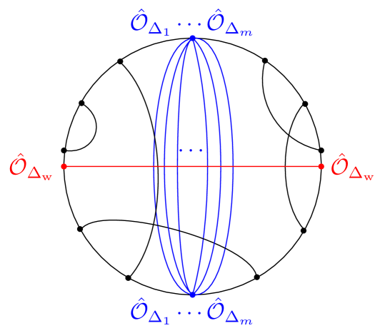
Figure 2: Example of the crossed chord diagram we evaluate in (32). The blue chords correspond to the composite operator $\prod_{i=1}^{m}\mathcal{O}_{\Delta_{i}}$, and the red chord to a pair of probe operators $\mathcal{O}_{\Delta_{w}}$.

Moreover, we can verify that the two-point correlation function corresponding to the two-sided HH state (7) in the one-particle irrep. is equivalent to a crossed four-point function with respect to $\mathcal{H}^{L}_{0}\otimes\mathcal{H}_{0}^{R}$. Consider $\tau_{L}=-\tau_{R}=\mathrm{i}t$,

$$\bra{\Psi_{\tilde{\Delta}}(-\mathrm{i}t,\mathrm{i}t)}q^{\Delta_{w}\hat{N}}\ket{\Psi_{\tilde{\Delta}}(-\mathrm{i}t,\mathrm{i}t)} =\bra{0}\hat{\mathcal{O}}_{\Delta_{\rm S}}(t)q^{\Delta_{w}\hat{N}}\hat{\mathcal{O}}_{\Delta_{\rm S}}(t)\ket{0}$$ (33)

$$=\langle 0|\hat{\mathcal{O}}_{\Delta_{\rm S}}(t)\leavevmode\hbox to5.56pt{\vbox to7.22pt{\text{[drawing]}}}_{\Delta_{w}}(0)\hat{\mathcal{O}}_{\Delta_{\rm S}}(t)\leavevmode\hbox to5.56pt{\vbox to7.22pt{\text{[drawing]}}}\leavevmode\hbox to0pt{\vbox to0pt{\text{[drawing]}}}_{\Delta_{w}}(0)|{0}\rangle\vbox to15.99992pt{}{}\leavevmode\nobreak\ , \hat{\mathcal{O}} \hat{\mathcal{O}}$$

where the bar denotes Wick contraction. Thus, we see that the two-sided two-point function is indeed an OTOC. A plot of the OTOC for all times is displayed in Fig. 3.

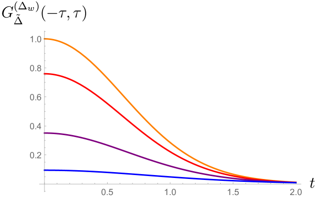
Figure 3: Evolution of the OTOC (32) for $\tau_{R}=-\tau_{L}=\frac{\beta(\theta)}{2}+\mathrm{i}t$. We are taking $\lambda\Delta_{\rm S}=1$, $J=1$, $\lambda=10^{-6}$, $\Delta_{w}=1$, and different values of $\theta$ starting from $\frac{\pi}{2}$ (orange) and decreasing in steps of $0.3$ (corresponding curves in descending order).

We study different properties of the OTOC in App. G.

2.4 Double-scaled precursor operators

Shockwaves lengths from chord diagram computations have been previously discussed in Berkooz:2022fso (albeit in the triple scaling limit). In this section, we explain how to derive the same type of distances from the Euclidean path integrals without the triple scaling limit. In the following, we consider how to recover single shockwave geometries from the one-particle HH state. We leave a comprehensive study with multiple shockwaves to future directions AX .

Double-scaled precursors

Motivated by the original definition in Stanford:2014jda (see also Berkooz:2022fso ), we introduce double-scaled precursor operators in the Schrödinger picture, as

$$\hat{\mathcal{O}}^{L}_{\Delta}(t_{w})\equiv\mathrm{e}^{\mathrm{i}t_{w}\hat{H}_{L}}\hat{\mathcal{O}}^{L}_{\Delta}\mathrm{e}^{-\mathrm{i}t_{w}\hat{H}_{L}}\leavevmode\nobreak\ ,$$ (34)

$$\hat{\mathcal{O}}^{R}_{\Delta}(t_{w})\equiv\mathrm{e}^{-\mathrm{i}t_{w}\hat{H}_{R}}\hat{\mathcal{O}}^{R}_{\Delta}\mathrm{e}^{\mathrm{i}t_{w}\hat{H}_{R}}\leavevmode\nobreak\ ,$$

where $t_{w}\in\mathbb{R}$ is the insertion time of the operator. The definition on (34) from the right chord sector corresponds to evolving an state in the past, inserting an operator and evolving by the same time scale. Note that transforming the matter chord operators for the precursor operators amounts to an overall time shift in factors of the form

$$\mathrm{e}^{-\tau_{L}\hat{H}_{L}-\tau_{R}\hat{H}_{R}}\hat{\mathcal{O}}_{\Delta}(t_{w})\ket{0} \mathrm{e}^{-(\beta_{L}-\mathrm{i}(t_{L}-t_{w}))\hat{H}_{L}}\hat{\mathcal{O}}^{L}_{\Delta}\mathrm{e}^{-(\frac{\beta_{R}}{2}+\mathrm{i}(t_{R}+t_{w}))\hat{H}_{L}}\ket{0}$$ (35)

$$=\mathrm{e}^{-(\frac{\beta_{R}}{2}-\mathrm{i}(t_{R}+t_{w}))\hat{H}_{R}}\hat{\mathcal{O}}_{\Delta}^{R}\mathrm{e}^{-(\frac{\beta_{L}}{2}+\mathrm{i}(t_{L}-t_{w}))\hat{H}_{R}}\ket{0}\leavevmode\nobreak\ .$$

This means that the double-scaled precursor operators (34) generate an overall time shift $t_{L}\rightarrow t_{L}-t_{w}$ and $t_{R}\rightarrow t_{R}+t_{w}$. In terms of the classical phase space solutions (29a), the replacement of $\hat{O}_{\Delta}$ for the precursor (34) shifts the initial conditions in (27) as

$$\evaluated{\ell}_{t_{L}=-t_{R}=t_{w}}=\ell_{*}(\theta_{L},\theta_{R})\leavevmode\nobreak\ ,\quad\evaluated{\derivative{\ell}{t_{L/R}}}_{t_{L}=-t_{R}=t_{w}}=0\leavevmode\nobreak\ .$$ (36)

where $\ell_{*}(\theta_{L},\theta_{R})$ was determined in (31) from the EOM and energy conservation. We can then express (29a) as

$$\ell=2\log\biggl(&\cosh(\gamma_{L}(t_{L}-t_{w})+\gamma_{R}(t_{R}+t_{w})){\\ }&+\quantity(\frac{J^{2}q^{\Delta_{\rm S}}\mathrm{e}^{-\ell_{*}}}{\gamma_{L}\gamma_{R}}-1)\sinh(\gamma_{L}(t_{L}-t_{w}))\sinh(\gamma_{R}(t_{R}+t_{w}))\biggr{missing})+\ell_{*}\leavevmode\nobreak\ .$$ (37)

Shockwave limit

We would like to study the shockwave limit, i.e. the regime where (37) has the same evolution as the wormhole geodesic distances as Shenker:2013pqa (we discuss the bulk interpretation in Sec. 4.2). In this picture, one has to consider a very early (meaning $t_{w}\rightarrow\infty$) perturbation of the TFD state. This implies that the system is always in an equal temperature ensemble, $\beta_{L}=\beta_{R}$, so that $\gamma_{L}=\gamma_{R}\equiv J\sin\theta$ (i.e. $\ell_{*}(\theta_{L},\theta_{R})=\ell_{*}^{+}(\theta)$ in (62)). Thus, the evolution of (37) for $t_{w}\gg t_{L/R}$ becomes

$$\ell(t_{L},t_{R})\simeq 2\log\biggl(\cosh(J\sin\theta(t_{L}+t_{R}))+\quantity(\frac{1}{4}-\frac{q^{\Delta_{\rm S}}\mathrm{e}^{-\ell_{*}^{+}(\theta)}}{4\sin^{2}\theta})\mathrm{e}^{-J\sin\theta(t_{L}-t_{R}-2t_{w})}\biggr{missing})$$ (38)

$$+\ell^{(+)}_{*}(\theta)\leavevmode\nobreak\ .$$

and the corresponding momenta (29a):

$${P_{L/R}=\mathrm{i}\log(\cos\theta+\mathrm{i}\sin\theta\frac{{\sin^{2}\theta}\tanh(\delta t_{L/R})+{q^{\Delta}\mathrm{e}^{-\ell_{*}^{(+)}}}\tanh(\delta t_{R/L})}{{\sin^{2}\theta}+{q^{\Delta}\mathrm{e}^{-\ell_{*}^{(+)}}}\tanh(\delta t_{L})\tanh(\delta t_{R})})\leavevmode\nobreak\ ,}$$ (39)

where

$$\delta t_{L}=J\sin\theta(t_{L}-t_{w})\leavevmode\nobreak\ ,\quad\delta t_{R}=-J\sin\theta(t_{R}+t_{w})\leavevmode\nobreak\ .$$ (40)

Note that the limiting behavior in (38) is only valid for $t_{w}\gg\absolutevalue{t_{L/R}}$. This is what allows us to consistently discard exponentially suppressed terms to arrive at (38).

Let us interpret the results so far. For instance, Krylov operator complexity ($t_{L}=-t_{R}$) (70) takes the same form as (38) after replacing $\ell^{(-)}_{*}\rightarrow\ell^{(+)}_{*}$ in (68). This corresponding to a different Wightman inner product than (169) where instead we take $\beta_{L}=\beta_{R}$. Moreover, there are solutions display a scrambling behavior (i.e. the transition from exponential to linear growth) when we consider the time regimes

$$\ell(t_{L},t_{R})\simeq\begin{cases}\quantity(\frac{1}{2}-\frac{q^{\Delta_{\rm S}}\mathrm{e}^{-\ell_{*}^{+}(\theta)}}{2\sin^{2}\theta})\mathrm{e}^{-J\sin\theta(t_{L}-t_{R}-2t_{w})}+\ell^{(+)}_{*}(\theta)\leavevmode\nobreak\ ,&t_{L}\gg\absolutevalue{t_{R}}\\ 2\log\quantity(\frac{1}{4}-\frac{q^{\Delta_{\rm S}}\mathrm{e}^{-\ell_{*}^{+}(\theta)}}{4\sin^{2}\theta})+J\sin\theta(t_{R}+2t_{w}-t_{L})+\ell^{(+)}_{*}(\theta)\leavevmode\nobreak\ ,&t_{R}\gg\absolutevalue{t_{L}}\leavevmode\nobreak\ .\end{cases}$$ (41)

We will discuss more on this limit and its place in the holographic dictionary in Sec. 4.2.For now, note that $t_{L}=t_{R}$ (associated with spread complexity) does not display scrambling (as observed in our discussion in Sec. 3.2). Additionally, the last entry in (41) obeys (4.7) in Stanford:2014jda for $n=1$.

3 The Krylov space of the two-sided Hartle-Hawking state

In this section, we connect our previous results on saddle points of the path integral with the Krylov complexity of the two-sided HH state.

Outline

In Sec. 3.1 we formulate the Lanczos algorithm for two-sided Hamiltonians that evaluates the Krylov operator complexity of the operator $\mathcal{O}_{\Delta}$, or the spread complexity of the two-sided HH state (7), depending on the relative time orientation in the Hamiltonian evolution, and that incorporates finite temperature effects. We derive the Lanczos coefficients and Krylov basis from the chord Hamiltonians. In Sec. 3.2 we apply the classical phase space results to deduce the semiclassical Krylov complexity. Then, Sec. 3.2 focuses on the properties of spread and Krylov operator complexity. Special cases in our results match with existing literature Ambrosini:2024sre ; Heller:2024ldz . An OTOC is the generator of Krylov operator complexity. It displays a scrambling behavior, i.e. a transition between exponential to late-time linear growth (in a similar way as in circuit complexity Chapman:2021jbh ; Susskind:2014rva ), inherited from scrambling in the OTOC. It is hyperfast, in the sense of Susskind:2021esx , and it is consistent with several bounds in the literature Maldacena:2015waa ; Anegawa:2024yia ; Milekhin:2024vbb . Lastly, in Sec. 3.3 we discuss how the Lanczos algorithm changes when we insert double-scaled precursor operators (34) to build the two-sided HH state, and its shockwave limit, introduced in Sec. 2.4.

3.1 Lanczos algorithm for two-sided Hamiltonians

In this subsection, we will show that the Krylov operator or spread complexity for matter chord operators or the two-sided HH state (7) respectively equals the expectation value of the total chord number with different time orientation in the semiclassical limit. We implement the Lanczos algorithm with two-sided Hamiltonians and finite temperatures based on the Lanczos algorithm for one-sided Hamiltonian with complex time evolution in Erdmenger:2023wjg , which we summarize in App. C.2. We first express the two-sided HH state (7) as

$$\ket{\Psi_{\tilde{\Delta}}(\tau_{L},\tau_{R})}=\mathrm{e}^{-\tau_{L}\hat{H}_{L}-\tau_{R}\hat{H}_{R}}\ket{\tilde{\Delta};0\dots,0}=\mathrm{e}^{-\tau_{R}\mathcal{L}_{\eta}}\ket{\Delta_{\rm S};0,0}\leavevmode\nobreak\ ,$$ (42)

where $\Delta_{\rm S}\equiv\sum_{i=1}^{m}\Delta_{i}$, and

$$\hat{\mathcal{L}}_{\eta}\equiv\hat{H}_{R}+\eta\hat{H}_{L}\leavevmode\nobreak\ ,\quad(\eta\equiv\tau_{L}/\tau_{R})$$ (43)

is a generalized Liouvillian operator for two-sided Hamiltonians. In principle, $\eta$ does not need to be a constant, and it could be complex. However, in order for the complex time generator $\mathcal{L}_{\eta}$ to be independent of $\tau_{L/R}$, we set $\eta$ to be constant; i.e. when

$$t_{R}=\eta t_{L}\leavevmode\nobreak\ ,\quad\beta_{R}=\eta\beta_{L}\leavevmode\nobreak\ .$$ (44)

The above definitions reproduce the usual Schrödinger and Heisenberg picture evolution for states and operators used in the Lanczos algorithm when we restrict the problem to $\eta=+1$ and $-1$ respectively.

State case: Given that we work with the two-sided HH state at an initial time

$$\ket{\Psi_{\Delta}\quantity(\tfrac{\beta_{L}}{2},\tfrac{\beta_{R}}{2})}=\mathrm{e}^{-\beta_{L}\hat{H}_{L}-\beta_{R}\hat{H}_{R}}\hat{\mathcal{O}}_{\tilde{\Delta}}\ket{0}\leavevmode\nobreak\ ,$$ (45)

Then, this state in the Schrödinger picture with a total Hamiltonian $\hat{H}_{L}+\hat{H}_{R}$, meaning

$$\mathrm{i}\partial_{t}\ket{\Psi_{\Delta}}=(\hat{H}_{L}+\hat{H}_{R})\ket{\Psi_{\Delta}}\leavevmode\nobreak\ ,$$ (46)

which is solved by (7) with $t_{L}=t_{R}=t$. For this reason, the Lanczos algorithm describes spread complexity (corresponding to the Schrödinger picture) when $t_{L}=t_{R}=t$. In principle, we do not require $\beta_{L}=\beta_{R}$; this is simply a simplification to threat the problem with a single complex time parameter $\tau$.

Operator case: As reviewed in App. C.2, the Liovillian operator, generating the evolution of an operator $\hat{\mathcal{O}}_{\Delta}^{L}\equiv\hat{\mathcal{O}}_{\Delta}\otimes\mathbb{1}$ in a two-sided Hamiltonian system can be expressed as $\hat{\mathcal{L}}=\hat{H}_{R}-\hat{H}_{L}$ (and $\hat{\mathcal{L}}=\hat{H}_{L}-\hat{H}_{R}$ for $\hat{\mathcal{O}}_{\Delta}^{R}\equiv\mathbb{1}\otimes\hat{\mathcal{O}}_{\Delta}$). We will use the Choi–Jamiołkowski isomorphism to represent the Heisenberg picture operator

$$\hat{\mathcal{O}}^{L/R}_{\Delta}(t)\equiv\mathrm{e}^{-\mathrm{i}\mathcal{L}t}\hat{\mathcal{O}}^{L/R}_{\Delta}=\mathrm{e}^{\mathrm{i}\hat{H}_{L/R}t}\hat{\mathcal{O}}^{L/R}_{\Delta}\mathrm{e}^{-\mathrm{i}\hat{H}_{L/R}t}\leavevmode\nobreak\ ,$$ (47)

into a state $\hat{\mathcal{O}}_{\Delta}(t)\ket{0}$. In order to define the Hilbert space of the states resulting from the above operator-state map, we need to specify their inner product, which in this case involves a thermal ensemble with arbitrary inverse temperatures $\beta_{L}$, $\beta_{R}$. There are different choices satisfying specific axioms, as reviewed in Nandy:2024htc ; Sanchez-Garrido:2024pcy in the one-sided Hamiltonian case. Given that there is no unique way to generalize the different choices of thermal ensemble inner product in two-sided Hamiltonian systems with different temperatures, we are free to choose any that satisfies the inner product space axioms Nandy:2024htc ; Sanchez-Garrido:2024pcy at this point, so for technical convenience we adopt $\mathrm{e}^{-\frac{\beta_{L}}{2}\hat{H}_{L}-\frac{\beta_{R}}{2}\hat{H}_{R}}\hat{\mathcal{O}}_{\tilde{\Delta}}$ as a single or composite operator that is mapped through the Choi–Jamiołkowski isomorphism to a state:

$$\mathrm{e}^{-\frac{\beta_{L}}{2}\hat{H}_{L}-\frac{\beta_{R}}{2}\hat{H}_{R}}\hat{\mathcal{O}}^{L/R}_{\Delta}(t)\rightarrow\mathrm{e}^{-\frac{\beta_{L}}{2}\hat{H}_{L}-\frac{\beta_{R}}{2}\hat{H}_{R}}\hat{\mathcal{O}}^{L/R}_{\Delta}(t)\ket{0}\leavevmode\nobreak\ ,$$ (48)

which comes equipped with the inner product in $\mathcal{H}_{m}$ (which in this case a $\mathcal{H}_{1}$ irrep).

Thus, we can treat the Krylov space problem for operators (173), (176) in the same way as for states in (164, 165). We have to perform the replacement $\hat{H}\rightarrow\hat{\mathcal{L}}$.

Both cases

We now work with a Krylov complexity measure labeled by $\eta$ for $t_{R}=\eta t_{L}$ (corresponding to spread or Krylov operator complexity when $\eta=+1$ or $-1$ respectively). Note that the requirement $\beta_{R}=\eta\beta_{L}$ is just a matter of technical convenience that allows us to find closed form expressions for the Lanczos coefficients and Krylov basis. One could use arbitrary values of $\beta_{R}$ and $\beta_{L}$ that are not necessarily related to each other, compared to (44). This essentially corresponds to a different choice of choice of thermal ensemble in the evaluation of the inner product, as seen in the previous cases. On the other hand, one is tempted to formulate new measures of Krylov complexity that interpolate between state and operator complexity by allowing $\eta\in\mathbb{R}$; however, we have not found a Krylov basis for $\eta\neq\pm 1$ that solves the Lanczos algorithm below. For this reason, we restrict the analysis to $\eta=\pm 1$.

We perform the decomposition of the two-sided HH state into its Krylov basis

$$\ket{\Psi_{\tilde{\Delta}}(\tau_{L}=\eta\tau,\tau_{R}=\tau)}=\sum_{n=0}^{\infty}\Psi^{(\eta)}_{n}(\tau)\ket{K^{(\eta)}_{n}}\leavevmode\nobreak\ ,$$ (49)

where $\Psi^{(\eta)}_{n}(\tau)\equiv\bra{K_{n}^{(\eta)}}\ket{\Psi_{\tilde{\Delta}}(\tau_{L}=\eta\tau,\tau_{R}=\tau)}$, and the orthonormal basis $\quantity{\ket{K_{n}^{(\eta)}}}$ is generated from the Lanczos algorithm

$$\hat{\mathcal{L}}_{\eta}\ket{K^{(\eta)}_{n}} \equiv(\hat{H}_{R}+\eta\hat{H}_{L})\ket{K^{(\eta)}_{n}}$$ (50)

$$=b^{(\eta)}_{n+1}\ket{K_{n+1}^{(\eta)}}+b^{(\eta)}_{n}\ket{K_{n-1}^{(\eta)}}+a_{n}^{(\eta)}\ket{K_{n}^{(\eta)}}\leavevmode\nobreak\ ,$$

where $\ket{K_{0}^{(\eta)}}=\ket{\tilde{\Delta};0,\dots,0}=\ket{{\Delta_{\rm S}};0,0}$ (by (9)). By demanding that $\eta$ in (44) is a fixed number, $\hat{\mathcal{L}}_{\eta}$ is $\tau$-independent. The amplitudes $\Psi^{(\eta)}_{n}(\tau)$ solve a Lanczos algorithm of the form:

$$-\partial_{\tau}\Psi^{(\eta)}_{n}(\tau)=b^{(\eta)}_{n+1}\Psi^{(\eta)}_{n+1}(\tau)+b^{(\eta)}_{n}\Psi^{(\eta)}_{n-1}(\tau)+a^{(\eta)}_{n}\Psi^{(\eta)}_{n}(\tau)\leavevmode\nobreak\ .$$ (51)

where $\Psi_{n}^{(\eta)}(\tau=\beta_{R})=Z_{\tilde{\Delta}}(\eta\beta,\beta)$.

The Krylov complexity operator, and its expectation value are just

$$\hat{\mathcal{C}} =\sum_{n}n\ket{K^{(\eta)}_{n}}\bra{K^{(\eta)}_{n}}\leavevmode\nobreak\ ,$$ (52)

$$\mathcal{C}^{(\eta)}(t) =\evaluated{\frac{\bra{\Psi_{\tilde{\Delta}}(\eta\tau,\tau)}\hat{\mathcal{C}}\ket{\Psi_{\tilde{\Delta}}(\eta\tau,\tau)}}{\bra{\Psi_{\tilde{\Delta}}(\eta\beta,\beta)}\ket{\Psi_{\tilde{\Delta}}(\eta\beta,\beta)}}}_{\tau=\frac{\beta}{2}+\mathrm{i}t}\leavevmode\nobreak\ .$$

To identify the specific Krylov basis corresponding to the two-sided HH state (7) with $\tau_{L}=\eta\tau_{R}$, we can make an ansatz where the total chord number is fixed by expanding the term $\mathrm{e}^{-\tau\hat{\mathcal{L}}_{\eta}}$ with the binomial theorem:

$$\ket{\Psi_{\tilde{\Delta}}(\tau_{L}=\eta\tau,\tau_{R}=\tau)}=\sum_{n=0}^{\infty}\frac{(-\tau)^{n}}{n!}\sum_{l=0}^{n}\begin{pmatrix}n\\ l\end{pmatrix}\eta^{l}\hat{H}_{L}^{l}\hat{H}_{R}^{n-l}\ket{\Delta_{\rm S};0,0}\leavevmode\nobreak\ ,$$ (53)

where, again, we denote $\Delta_{\rm S}=\sum_{i=1}^{m}\Delta_{i}$. Using the normal ordering prescription of Xu:2024hoc ,

$$\ket{\Delta;n_{1},n_{2}}=:\hat{H}_{L}^{n_{1}}\hat{\mathcal{O}}_{\Delta}\hat{H}_{R}^{n_{2}}:\ket{0}\leavevmode\nobreak\ ,$$ (54)

one can then build a fixed total chord number basis corresponding to (53) (which in does not necessarily need to be a Krylov basis):

$$\ket{k^{(\eta)}_{n}} =c^{(\eta)}_{n}\sum_{l=0}^{n}\eta^{k}\begin{pmatrix}n\\ l\end{pmatrix}\ket{\Delta_{\rm S};l,n-l}\leavevmode\nobreak\ ,$$ (55)

where $c_{n}^{(\eta)}$ is a normalization constant, shown explicitly in (249). The basis becomes orthonormal in the semiclassical limit, in the sense of $\bra{k^{(\eta)}_{n}}\ket{k^{(\eta)}_{m}}\underset{\lambda\rightarrow 0}{=}\delta_{nm}$ (as shown in App. H).

However, it is not guaranteed that $\quantity{\ket{k^{(\eta)}_{n}}}$ solves the Lanczos algorithm (50) which defines the Krylov basis $\quantity{\ket{K^{(\eta)}_{n}}}$ (hence the different notation). Thus,

$$\frac{\bra{\Psi_{\tilde{\Delta}}(\eta\tau,\tau)}\hat{N}\ket{\Psi_{\tilde{\Delta}}(\eta\tau,\tau)}}{\innerproduct{\Psi_{\tilde{\Delta}}(\eta\beta,\beta)}{\Psi_{\tilde{\Delta}}(\eta\beta,\beta)}} =(Z_{\tilde{\Delta}}(\eta\beta,\beta))^{-1}\sum_{n=0}^{\infty}n\absolutevalue{\innerproduct{k^{(\eta)}_{n}}{\Psi_{\tilde{\Delta}}(\eta\tau,\tau)}}^{2}\leavevmode\nobreak\ ,$$ (56)

does not need to represent Krylov complexity. It was shown in Ambrosini:2024sre that only in the exact semiclassical regime the total chord number basis corresponds to the Krylov basis for $\ket{\Delta;0,0}$ as the initial state in the Lanczos algorithm with $t_{L}=\pm t_{R}$ and at infinite temperature. In App. H, we show that the Krylov basis for the two-sided HH state in (7) is given by the normal ordering prescription basis $\quantity{\ket{k^{(\eta)}_{n}}}$ in (55) in the semiclassical limit $\lambda\rightarrow 0$ (while $n\lambda$ is held fixed). This means that $\ket{K_{n}^{(\eta)}}\underset{\lambda\rightarrow 0}{=}\ket{k_{n}^{(\eta)}}$ up to the addition of a state whose norm is negligible in the semiclassical limit.

The Lanczos coefficients are found in (248). Thus, the Krylov complexity for a time orientation $t_{L}=\pm t_{R}$ and temperature $\beta_{L}=\pm\beta_{R}$ in the $\mathcal{H}_{m}$ double-scaled PETS (7) indeed is given by the expectation value in (56), at least in the $\lambda\rightarrow 0$ regime. We also deduced simplified the amplitudes entering in the Lanczos algorithm (50); see (253) for the details.

3.2 Krylov complexity in the two-sided Hartle-Hawking state

Following the discussion in Sec. 3.1, (29a) represents spread complexity (i.e. $\tau_{L}=\tau_{R}$) and Krylov operator complexity (i.e. $\tau_{L}=-\tau_{R}$). This means:

$$\lambda\leavevmode\nobreak\ \mathcal{C}^{(\eta)}(t)\equiv\ell(t_{L}=\eta t,t_{R}=t)\leavevmode\nobreak\ .$$ (57)

We notice that the non-zero initial value for Krylov complexity $\mathcal{C}^{(\eta)}(t=0)=\ell_{*}/\lambda$ in a HH preparation of state can be interpreted as the survival amplitude for $\ket{0}$ to remain unchanged during its evolution. This has been discussed in Erdmenger:2023wjg ; Balasubramanian:2022tpr for spread complexity in finite dimensional quantum systems.

Furthermore, since the chord number operator corresponds to Krylov complexity operator in the semiclassical regime ($\lambda\rightarrow 0$), it follows that the Krylov complexity generating function is exactly given by the thermal two-point correlation function in (232) when $t_{L}=\eta t_{R}$, $\beta_{L}=\eta\beta_{R}$,

$$G^{(\Delta_{w})}_{\tilde{\Delta}}(\tau_{L}=\eta\tau,\tau_{R}=\tau)=\frac{\bra{\Psi_{\tilde{\Delta}}(\eta\tau,\tau)}q^{\Delta_{w}\hat{N}}\ket{\Psi_{\tilde{\Delta}}(\eta\tau,\tau)}}{\bra{\Psi_{\tilde{\Delta}}(\eta\beta,\beta)}\ket{\Psi_{\tilde{\Delta}}(\eta\beta,\beta)}}\leavevmode\nobreak\ .$$ (58)

Here $\hat{N}=\hat{n}_{L}+\hat{n}_{1}+\dots+\hat{n}_{m-1}+\hat{n}_{R}$. We can look for the Krylov complexity moments encoded in (58) (where Krylov complexity corresponds to the first moment) using

$$\expectationvalue{\hat{\mathcal{C}}^{k}}\underset{\lambda\rightarrow 0}{=}\evaluated{\quantity(\frac{-1}{\lambda})^{k}\frac{\partial^{k}}{\partial\Delta_{w}^{k}}G^{(\Delta_{w})}_{\tilde{\Delta}}(\eta\tau,\tau)}_{\Delta_{w}=0}\leavevmode\nobreak\ .$$ (59)

Now, we would like to determine Krylov complexity for states and operators with temperature dependence from the two-sided HH state (7). Following our discussion in Sec. 3.1, we stress that the dynamical distance variable (29a) that we have derived from classical phase space only has a clear interpretation as semiclassical Krylov complexity (i.e. it has a Krylov basis obeying the Lanczos algorithm (50)) when we demand that both $t_{L}=\eta t_{R}\equiv\eta t$ and $\beta(\theta_{L})=\eta\beta(\theta_{R})\equiv\eta\beta(\theta)$ for $\eta=\pm 1$. This places restrictions on the relationship between the angular parameterization of the energy spectrum of the left and right chord sectors (i.e. in $E_{L/R}=E(\theta_{L/R})$ (137)).

Spread complexity

In the particular case where $t_{L}=t_{R}$, we require $\beta(\theta_{L})=\beta(\theta_{R})$, where the microcanonical inverse temperature ((148)) with $n=0$)

$$\beta(\theta)=2\frac{\pi-2\theta}{J\sin\theta}\leavevmode\nobreak\ ,$$ (60)

which for $\theta_{L/R}\in[0,\pi]$ (60) implies $\theta_{L}=\theta_{R}\equiv\theta$. This condition in (31) implies that $\ell_{t_{L}=t_{R}=0}(0)=\ell_{m}(t_{L}=t_{R}=0)\equiv\ell^{(+)}_{*}/2$ since they satisfy the same equation. The initial distance becomes

$$\mathrm{e}^{-\frac{1}{2}\ell^{(+)}_{*}(\theta)}=\frac{q^{-\Delta_{\rm S}}}{2}\quantity(-1+q^{\Delta_{\rm S}}+\sqrt{1+q^{2{\Delta_{\rm S}}}-2q^{\Delta_{\rm S}}\cos 2\theta})\leavevmode\nobreak\ .$$ (61)

Thus, the corresponding spread complexity for states of the form

$$\mathrm{e}^{-\quantity(\frac{\beta(\theta)}{2}+\mathrm{i}t)(\hat{H}_{L}+\hat{H}_{R})}\hat{\mathcal{O}}_{\Delta_{1}}\dots\hat{\mathcal{O}}_{\Delta_{m}}\ket{0}\leavevmode\nobreak\ ,$$ (62)

at leading order as $\lambda\rightarrow 0$ ($\frac{\lambda}{1-q}\rightarrow 1$) is then given by (29a) with $t_{L}=t_{R}$ and $\beta_{L}=\beta_{R}$, i.e.:

$$\mathcal{C}^{(\eta=+1)}(t)=\frac{2}{\lambda}\log\quantity(1+\quantity(1+\frac{\mathrm{e}^{-\ell^{(+)}_{*}(\theta)}q^{\Delta_{\rm S}}}{\sin^{2}\theta})\sinh^{2}\quantity(J\sin\theta\leavevmode\nobreak\ t))+\frac{\ell^{(+)}_{*}(\theta)}{\lambda}$$ (63)

$$=\frac{2}{\lambda}\log(A(\theta,q^{\Delta_{\rm S}})+B(\theta,q^{\Delta_{\rm S}})\cosh(2J\sin\theta t))\leavevmode\nobreak\ .$$

where $\ell^{(+)}_{*}(\theta)$ was defined in (62), and

$$A(\theta,q^{\Delta})=\frac{(\cos\theta-\cos 2\theta)q^{\Delta}+\left(1-q^{\Delta}\right)\left(q^{\Delta}+\sqrt{q^{2\Delta}-2\cos\theta q^{\Delta}+1}-1\right)}{2\sin^{2}\theta\left(q^{\Delta}+\sqrt{q^{2\Delta}-2\cos\theta q^{\Delta}+1}-1\right)}\leavevmode\nobreak\ ,$$ (64)

$$B(\theta,q^{\Delta})=\frac{q^{2\Delta}-\left((\cos\theta+\cos 2\theta)q^{\Delta}\right)-\left(1-q^{\Delta}\right)\sqrt{q^{2\Delta}-2\cos\theta q^{\Delta}+1}+1}{2\sin^{2}\theta\left(q^{\Delta}+\sqrt{q^{2\Delta}-2\cos\theta q^{\Delta}+1}-1\right)}\leavevmode\nobreak\ .$$ (65)

We can notice that (70) displays a transition between parabolic to late-time linear growth.

Comparison with the literature

We can now compare the result with the existing literature. (63) agrees with (4.16) in Ambrosini:2024sre when we consider a one-particle chord and $\theta=\pi/2$ (corresponding to an infinite temperature limit, where $\ell^{(+)}_{*}=0$ from (61)). This means that (29a) is also supported by the numerical evaluation of Krylov complexity for perturbations of the TFD state at infinite temperature in Ambrosini:2024sre . Furthermore, the expression (63) with ${\Delta}_{1}=\cdots=\Delta_{m}=0$ and $J=1$ also matches Heller:2024ldz . where $\mathrm{e}^{-\ell^{(+)}_{*}}\rightarrow\sin^{2}\theta$.

Krylov operator complexity

For Krylov operator complexity, we recover a Lanczos algorithm of the form (51) when $t_{L}=-t_{R}\equiv-t$ and

$$\frac{2(\pi-2\theta_{L})}{\sin\theta_{L}}=-\frac{2(\pi-2\theta_{R})}{\sin\theta_{R}}\leavevmode\nobreak\ ,$$ (66)

i.e. $\beta(\theta_{L})=-\beta(\theta_{R})$. This condition is satisfied by $\theta_{R}=\pi-\theta_{L}$; which implies that the parameter $\sin\theta_{L}=\sin\theta_{R}\equiv\sin\theta$ (i.e. $\gamma_{L}=\gamma_{R}$ (30)). This means that

$$\ell_{0}(t_{L}=t_{R}=0)=\ell_{m}(t_{L}=t_{R}=0)=\ell^{(-)}_{*}/2$$ (67)

as the initial condition in (31) (which relates the initial total distance variable with the energy of the left/right chord sectors). Denoting $\theta_{R}=\pi-\theta_{L}\equiv\theta$, (31) becomes

$$\mathrm{e}^{-\frac{1}{2}\ell^{(-)}_{*}(\theta)}=\frac{q^{-\Delta_{\rm S}}}{2}\quantity(1+q^{\Delta_{\rm S}}-\sqrt{1+q^{2\Delta_{\rm S}}+2q^{\Delta_{\rm S}}\cos 2\theta})\leavevmode\nobreak\ .$$ (68)

Thus, using the Choi–Jamiołkowski isomorphism (App. C.2), we can feed the Lanczos algorithm (50) with reference (Heisenberg picture) operators of the form

$$\mathrm{e}^{-\quantity(\frac{\beta(\theta)}{2}+\mathrm{i}t)(\hat{H}_{R}-\hat{H}_{L})}\hat{\mathcal{O}}_{\Delta_{1}}\dots\hat{\mathcal{O}}_{\Delta_{m}}\leavevmode\nobreak\ ,$$ (69)

to recover the Krylov operator complexity (29a) at leading order in the $\lambda\rightarrow 0$ limit

$$\mathcal{C}^{(\eta=-1)}(t) =\frac{2}{\lambda}\log\quantity(1+\quantity(1-\frac{\mathrm{e}^{-\ell^{(-)}_{*}(\theta)}q^{\Delta_{\rm S}}}{\sin^{2}\theta})\sinh^{2}\quantity(J\sin\theta\leavevmode\nobreak\ t))+\frac{\ell^{(-)}_{*}(\theta)}{\lambda}$$ (70)

$$=\frac{2}{\lambda}\log\quantity(A(\theta,-q^{\Delta_{\rm S}})+B(\theta,-q^{\Delta_{\rm S}})\cosh(2J\sin\theta\leavevmode\nobreak\ t))\leavevmode\nobreak\ ,$$

where $A(\theta,q^{\Delta})$, $B(\theta,q^{\Delta})$ are shown in (64), (65). One can see that (70) experiences parabolic to exponential growth as captured by

$$\mathcal{C}^{(\eta=-1)}(t)\simeq \frac{1}{\lambda}\frac{\sin^{2}\theta-q^{\Delta_{\rm S}}\mathrm{e}^{-\ell_{*}^{(-)}}}{2\sin^{2}\theta}(2J\sin\theta\leavevmode\nobreak\ t)^{2}+\frac{\ell^{(-)}_{*}(\theta)}{\lambda}$$ (71a)

$$\text{when}\quad t\ll(J\sin\theta)^{-1}\leavevmode\nobreak\ ,$$

$$\mathcal{C}^{(\eta=-1)}(t)\simeq \frac{1}{\lambda}\frac{\sin^{2}\theta-\mathrm{e}^{-\ell^{(-)}_{*}(\theta)}q^{\Delta_{\rm S}}}{\sin^{2}\theta+\mathrm{e}^{-\ell^{(-)}_{*}(\theta)}q^{\Delta_{\rm S}}}\mathrm{e}^{2J\sin\theta\leavevmode\nobreak\ t}+\frac{2}{\lambda}\log(\frac{\sin^{2}\theta+\mathrm{e}^{-\ell^{(-)}_{*}(\theta)}q^{\Delta_{\rm S}}}{2\sin^{2}\theta})\leavevmode\nobreak\$$ (71b)

$$+\frac{\ell^{(-)}_{*}(\theta)}{\lambda}\leavevmode\nobreak\ \quad\text{when}\quad\frac{1}{J\sin\theta}\ll t\ll t_{\rm sc}\leavevmode\nobreak\ ,$$

where $t_{\rm sc}$ is the transition time such that $\frac{\sin^{2}\theta-\mathrm{e}^{-\ell^{(-)}_{*}}q^{\Delta_{\rm S}}}{\sin^{2}\theta+\mathrm{e}^{-\ell^{(-)}_{*}}q^{\Delta_{\rm S}}}\mathrm{e}^{2J\sin\theta\leavevmode\nobreak\ t}\approx 1$,

$$t_{\rm sc}=-\frac{1}{2J\sin\theta}\log\frac{{\sin^{2}\theta}-{\mathrm{e}^{-\ell^{(-)}_{*}(\theta)}}q^{\Delta_{\rm S}}}{2\quantity({\sin^{2}\theta}+{\mathrm{e}^{-\ell^{(-)}_{*}(\theta)}}q^{\Delta_{\rm S}})}\leavevmode\nobreak\ ,$$ (72)

where $\ell_{*}^{(-)}$ is in (68). At later times than the above scale, there is a transition to linear growth at

$$\mathcal{C}^{(\eta=-1)}(t)\simeq \frac{1}{\lambda}\quantity(\ell^{(-)}_{*}(\theta)+{4}J\sin\theta\leavevmode\nobreak\ t+2\log(\frac{\sin^{2}\theta-\mathrm{e}^{-\ell^{(-)}_{*}(\theta)}q^{\Delta_{\rm S}}}{4\sin^{2}\theta}))\leavevmode\nobreak\ ,\quad t\gg t_{\rm sc}\leavevmode\nobreak\ .$$ (73)

We display a plot of Krylov operator complexity for heavy operators in Fig. 4.

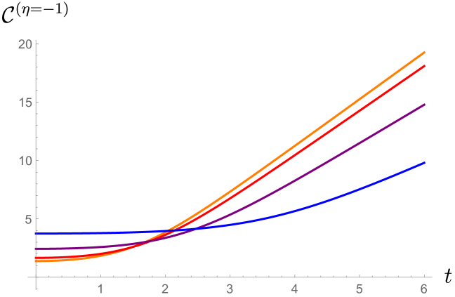
Figure 4: Krylov operator complexity (70). We are taking $\lambda=0.001$, $\lambda\Delta_{\rm S}=1$, $J=1$, and $\theta$ decreases from $\theta=\pi/2$ (orange) in multiples of $0.3$ from top to bottom at late times. Notice the exponential growth (71b) at the time scale below the scrambling time (72), followed by late time linear growth.

Comparison with the literature

It can be seen that (63) agrees with Ambrosini:2024sre when $\theta=\pi/2$ (corresponding to an infinite temperature limit, where $\ell^{(-)}_{*}=0$ from (61)). This means that (70) (and spread complexity in the previous section) at infinite temperature is also supported by their numerics. (70) exhibits an early time parabolic growth, followed by exponential growth and late-time linear growth. In fact, the results can be mapped to (3.85) in Ambrosini:2024sre with replacements $J\rightarrow J\sin\theta$, $\tilde{q}\rightarrow\mathrm{e}^{-\ell^{(-)}_{*}(\theta)}\frac{q^{\Delta_{\rm S}}}{\sin^{2}\theta}$.

Relation with quantum ergodic theory

We remark that the generator of Krylov operator complexity in (59) is the OTOC we investigated in (241). As we saw, the OTOC experiences a scrambling transition, which is indeed the scrambling time in Krylov operator complexity. Both can be used as notions of quantum chaos in this system. Moreover, there is a closely related notion, mixing in quantum ergodic theory (see e.g. Camargo:2025zxr ; Gesteau:2023rrx ; Furuya:2023fei ), which quantifies the degree of independence between elements in the operator algebra of a quantum system. In the simplest case, given two operators in the Heisenberg picture $\hat{A}$ and $\hat{B}(t)$, a quantum system is said to be 2-mixing when the cumulant (in this case a connected two-point function)

$$F_{2}(t)\equiv\expectationvalue{\hat{A}\hat{B}(t)}_{\varphi}-\expectationvalue{\hat{A}}_{\varphi}\expectationvalue{\hat{B}(t)}_{\varphi}\leavevmode\nobreak\$$ (75)

vanishes at late times, i.e.

$$\lim_{t\rightarrow\infty}F_{2}(t)=0\leavevmode\nobreak\ ,$$ (76)

and where $\ket{\varphi}$ is a normal state, which allows for continuous expectation values with respect to ultraweak topology Camargo:2025zxr .

In the case of the DSSYK model, we note that if we select matter chord operators to generate the connected two-point functions, i.e. $\hat{A}=\hat{\mathcal{O}}_{\Delta_{1}}$, and $\hat{B}(t)=\hat{\mathcal{O}}_{\Delta_{2}}(t)$, then $\expectationvalue{\hat{A}}_{\varphi}=\expectationvalue{\hat{B}(t)}_{\varphi}=0\leavevmode\nobreak\ \forall\ket{\varphi}\in\mathcal{H}_{m}$, while

$$\lim_{t\rightarrow\infty}F_{2}(t)=0\leavevmode\nobreak\ \forall\leavevmode\nobreak\ \varphi\in\mathcal{H}_{0}\leavevmode\nobreak\ \text{or}\leavevmode\nobreak\ \mathcal{H}_{1}\leavevmode\nobreak\ .$$ (77)

The case $\mathcal{H}_{0}$ follows immediately from known results in the literature (see e.g. (150)). Meanwhile, the $\mathcal{H}_{1}$ case follows from the late time regime of (241). In fact the mixing of the system applies more generally to $\mathcal{H}_{m}$, as we will see in in AX . Therefore, despite the DSSYK model having a continuous energy spectrum, it still displays signatures of quantum chaos, where the Krylov complexity, OTOC, and quantum hierarchy all agree with each other and they allow for an interpretation of chaos in the DSSYK.

Universal operator growth hypothesis

We also emphasize that the Krylov operator complexity in (70) is in agreement with the universal operator growth hypothesis (UOGH) Parker:2018yvk . The UOGH states that Krylov operator complexity grows at a rate $\mathrm{e}^{\frac{4\pi}{\beta}t}$, with $\beta$ being the inverse temperature of the system. As we saw (70) can at most grow exponentially (before the scrambling time in (71b)). In this regime, the UOGH is explicitly saturated when we consider the fake temperature of the DSSYK model (defined as the decay rate of two-point correlation functions Blommaert:2024ydx ), and undersaturated for the physical temperature (except at $\theta=0$),

$$\frac{4\pi}{\beta_{\rm fake}}={2J}\sin\theta\leavevmode\nobreak\ ,\quad\text{vs}\quad\frac{4\pi}{\beta(\theta)}=\frac{2J}{\absolutevalue{1-2\theta/\pi}}\sin\theta\leavevmode\nobreak\ .$$ (78)

Thus, the Lyapunov exponent for Krylov operator complexity, as well as its generating function (an OTOC with respect to $\mathcal{H}_{0}$) displays sub-maximal or maximal scrambling depending on whether we compare the Lyapunov exponent to the physical or fake temperature respectively.

Later evolution

Lastly, while (72) displays eternal late-time linear growth, it is also expected that at very late times Krylov complexity and other measure of quantum complexity will saturate, when considering finite-dimensional quantum systems instead of the ensemble theory we considered.

3.3 Krylov complexity for precursor operators

As we remarked in Sec. 2.4 the addition of the double-scaled precursor (34) translates into a time shift $t_{L}\rightarrow t_{L}-t_{w}$ and $t_{R}\rightarrow t_{R}+t_{w}$; which means that all the results we have derived in Sec. 3.1 are unaffected under the replacement of particle to precursor operator: $\hat{\mathcal{O}}^{L/R}_{\Delta}\rightarrow\hat{\mathcal{O}}^{L/R}_{\Delta}(t_{w})$ in (34). This implies that the two-sided HH state (7) transforms

$$\ket{\Psi_{\tilde{\Delta}}(\tau_{L},\tau_{R})}\rightarrow\ket{\Psi_{\tilde{\Delta}}(\tau_{L}-\mathrm{i}t_{w},\tau_{R}+\mathrm{i}t_{w})}\leavevmode\nobreak\ .$$ (79)

Thus, in order to apply our Lanczos algorithm (51), we simply need to work with shifted variables variables, such as

$$\tilde{\tau}_{L}=\frac{\beta_{L}}{2}+\mathrm{i}(t_{L}-t_{w})\leavevmode\nobreak\ ,\quad\tilde{\tau}_{R}=\frac{\beta_{R}}{2}+\mathrm{i}(t_{R}+t_{w})\leavevmode\nobreak\ ,$$ (80)

and impose that $\tilde{\eta}\equiv\tilde{\tau}_{L}/\tilde{\tau}_{R}$ is fixed to recover the same semiclassical Lanczos coefficients (50), Krylov basis (55) , and Krylov complexity (29a) (with $t_{L}\rightarrow t_{L}-t_{w}$ and $t_{R}\rightarrow t_{R}+t_{w}$).

Note however, that in the case of interest in Shenker:2013pqa , seen as a early time perturbation of the TFD state, we need to set $\beta_{L}=\beta_{R}$ ($E(\theta_{L})=E(\theta_{R})$), and $t_{w}\rightarrow\infty$. So the results of the Lanczos algorithm (51) in (50, 55, 29a) apply immediately only when $\beta_{L}=\beta_{R}=0$ for $t_{L}\neq t_{R}$; or when $\eta=+1$ (the spread complexity case) However, we stress that is is not necessary to fix $\beta_{L}=\eta\beta_{R}=\beta(\theta)$. The Lanczos coefficients (50) and Krylov basis (55), and Krylov complexity will depend on the parameter $\beta(\theta)$, such as what we find in (3.3).

4 The holographic dictionary and the dual double-scaled algebra

In this section, we derive the holographic dictionary for the DSSYK model with a one-particle insertion, considering a Schrödinger equation (101) for states in the bulk Hilbert space and also momentum shift symmetry (106); we perform the constraint quantization of the bulk dual theory; and we formulate the double-scaled algebra in bulk terms.

Deriving the holographic dictionary from Krylov complexity

Recent works have found a precise match between spread complexity in the DSSYK model with a minimal geodesic length in an (effective) AdS₂ black hole background without matter Rabinovici:2023yex ; Heller:2024ldz . Previous literature also found that Krylov operator complexity in the finite N SYK model is closely related to the minimal volume in an AdS₂ black hole geometry in JT gravity Jian:2020qpp . This motivates a closer inspection of Krylov complexity as a realization of the CV proposal by Susskind:2014rva ; Stanford:2014jda . A natural expectation is that our results from Sec. 3 should have a bulk interpretation in JT gravity or sine dilaton gravity with matter. Indeed, “wormhole distances”, i.e. minimal geodesic lengths between the asymptotic boundaries in an AdS black hole match the Krylov operator and spread complexity in Sec. 3. In particular, Krylov operator complexity has promising properties expected of holographic complexity proposals Belin:2021bga ; Belin:2021bga , as we explain in AX .

On the role of chord diagrams

One can also interpret the equality between the semiclassical Krylov operator complexity and the geodesic distance $L_{\rm AdS}$ from the holographic dictionary relating crossed four-point correlation functions in the DSSYK model (calculated from chord diagrams in Sec. E) with two-sided two-point correlation functions in the bulk, as previously realized in Berkooz:2022fso (albeit under different considerations). This means

$$\expectationvalue{q^{\Delta\hat{N}}}=\expectationvalue{\mathrm{e}^{-m_{\xi}L_{\rm AdS}}}\leavevmode\nobreak\ .$$ (81)

The expectation values above are evaluated in the two-sided HH state in the boundary and bulk sides, and they are normalized by the partition function of the thermal ensemble. From (81) when we identify $\lambda\leavevmode\nobreak\ \mathcal{C}=L_{\rm AdS}$ (in the regime $\lambda\rightarrow 0$). We are also identifying $\Delta=m_{\xi}$ in the holographic dictionary.

Thus, we see that there are different ways of filling in the holographic dictionary. Namely, chord diagrams, path integrals and Krylov complexity are all closely related, since the chord diagram Hamiltonian is the input for path integral, and the Lanczos algorithm. For this reason, it might be unsurprising they all yield equivalent results for the dual bulk geodesics in the semiclassical limit.

Outline

We tackle this problem by matching our previous results on saddle point solutions of the DSSYK path integral as semiclassical Krylov complexity in terms of minimal length geodesics in the bulk. In Sec. 4.1, we consider an AdS₂ black hole with a minimally coupled massive scalar field generating a small backreaction. We match the minimal geodesic length between the asymptotic boundaries to the Krylov operator complexity of the matter chord operator generating the two-sided HH state (7). We derive its holographic dictionary. Later, in Sec. 4.2 we study a shockwave geometry in an AdS₂ black hole. We derive a non-perturbative match between the minimal geodesic length connecting the asymptotic boundaries and Krylov operator and state complexity. The two types of Krylov complexity for the two-sided HH state represent different relative boundary time evolution for the minimal length geodesics. In Sec. 4.3 we perform the reduced phase space quantization of the bulk theory, sine-dilaton gravity, and we comment on the Dirac quantization. Following from our derivation of the holographic dictionary, we formulate the bulk dual double-scaled algebra; the main outcome of this work. In Sec. 4.4 we conclude exploring the relation between our results on the geometric interpretation of Krylov complexity and the proper radial momentum of a probe particle in the bulk, motivated by recent developments Caputa:2024sux .

4.1 Minimal length geodesic with a massive particle in AdS₂

As a warm-up, we will discuss about the bulk interpretation for Krylov operator complexity of the two-sided HH state (7) in terms of minimal geodesic lengths in AdS₂ with a massive particle insertion. We explore this first as this calculation is perturbative, while for the shockwave distance we can get a non-perturbative matching between semiclassical total chord number with AdS₂ geodesic lengths and not limited to the case $t_{L}=-t_{R}$. However, since the shockwave case is a particular type of backreaction in the bulk, the goal of this subsection is to see if there is a more generic type of backreaction that reproduces the same observable, after which we will specialize in shockwave case (Sec. 4.2).

Thus, following our discussion on the holographic dynamical properties captured by Krylov complexity, we search for a bulk interpretation of the results so far, and in particular, to confirm if (29a) describes the dynamics of a wormhole distance corresponding to Krylov complexity of the two-sided HH state (7). By wormhole distance, we refer to a geodesic distance between boundary particles with different time orientations; namely $t_{R}=\eta t_{L}$ with $\eta=\pm 1$ correspond to Krylov complexity in the semiclassical limit shown in Fig. 5. More general saddle point solutions to the Euclidean path integral (24) describe other time orientations. For this reason, we will study AdS₂ black hole geometries with matter operator insertions in this subsection and match the saddle points with the corresponding wormhole distance. We remark that the computations are valid for a general backreacted hyperbolic AdS₂ geometry by a minimally coupled massive field; which is precisely that for the massive scalar field in sine dilaton gravity (89). We will find that Krylov operator complexity (70) indeed reproduces the geodesic distance depicted in Fig. 5 (b) (albeit the bulk side of the calculation is perturbative); while spread complexity (63), does not precisely match with the corresponding geodesic distance ($t_{L}=t_{R}$) beyond the $\lambda\rightarrow 0$ limit.

A possible description of the double-scaled PETS in bulk terms, similar to the finite $N$ SYK case Goel:2018ubv is that the two-sided HH state (7) are constructed by inserting an operator in the Euclidean boundary of the geometry that bisects the interior, as shown in Fig. 5.

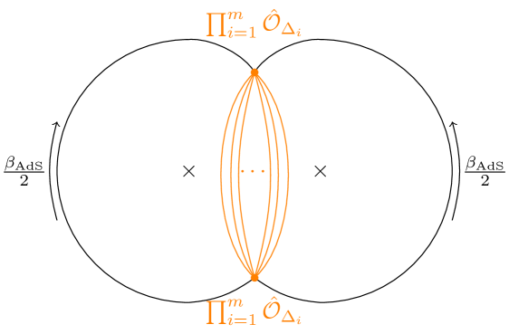
(a)

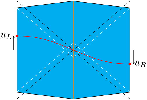
(b)

Figure 5: Bulk interpretation of the double-scaled PETS (7) described by the dual quantum system (16a, 16b). (a): Representation of the thermal partition function $Z_{\tilde{\Delta}}(-\beta,\beta)=\bra{\Psi_{\tilde{\Delta}}(-\beta,\beta)}\ket{\Psi_{\tilde{\Delta}}(-\beta,\beta)}$, where $\prod_{i}\hat{\mathcal{O}}_{\Delta_{i}}$ are inserted at the Euclidean boundary (orange dots), causing backreaction in the putative Euclidean bulk geometry, and dividing it into left and right sectors of the thermal circle with fake periodicity $\beta_{\rm fake}^{R}=\beta_{\rm fake}^{L}=\beta_{\rm AdS}/2$. The crosses, $\times$, represent the location of the conical singularities. (b): Lorentzian continuation. The operator insertions are collapsed to a single line (orange), and the curve joining the asymptotic boundaries (in red) represents the wormhole distance $(Z_{\tilde{\Delta}}(-\beta,\beta))^{-1}\bra{\Psi_{\tilde{\Delta}}(-\tau,\tau)}\hat{\ell}\ket{\Psi_{\tilde{\Delta}}(-\tau,\tau)}$ (29a), where $\tau=\beta+\mathrm{i}t$. Dashed white lines denote the location of the black hole horizons of the AdS geometries without backreaction from the massive particle, and the black dashed line the location of the event horizon with backreaction.

In Lorentzian signature, we consider AdS₂ black holes

$$\mathrm{d}s_{\rm AdS}^{2}=-f_{L/R}(r)\mathrm{d}u_{L/R}^{2}+\frac{\mathrm{d}r^{2}}{f_{L/R}(r)}\leavevmode\nobreak\ ,$$ (82)

$$f_{L/R}(r)=r^{2}-\quantity(\Phi_{h}^{L/R})^{2}\leavevmode\nobreak\ ,$$

where $r=\Phi_{h}^{L/R}={2\pi}/{\beta_{\rm AdS}^{L/R}}$ is the location of the event horizon, and $\beta_{\rm AdS}^{L/R}$ the inverse temperature. We allow for $\beta_{\rm AdS}^{L}$ and $\beta_{\rm AdS}^{R}$ to be independent of each other. Meanwhile, from the boundary side, we require $\beta_{L}=-\beta_{R}$ (Sec. 3.1) in order for the Krylov operator complexity (computed from the algorithm (50)) to have a semiclassical description in terms of an expectation value of the total chord number. However, why should there be negative temperatures in the bulk? We interpret this in terms of fake vs real temperature in sine dilaton gravity Blommaert:2024ydx , where the inverse temperature in the effective AdS₂ geometry (82) corresponds to the decay rate of thermal two-point correlation functions, given in (78), instead of the real DSSYK inverse temperature, which we derived in (188) (with $n=0$ for the thermodynamically stable saddle point). Comparing these relations,

$$\beta_{\rm fake}(\theta_{L/R})=\frac{\pi}{J\sin\theta_{L/R}}\leavevmode\nobreak\ ,\quad\text{vs}\quad\beta_{L/R}=\beta(\theta_{L/R})=\frac{\pi-2\theta_{L/R}}{J\sin\theta_{L/R}}\leavevmode\nobreak\ ,$$ (83)

we notice that $J\beta_{\rm fake}(\theta_{L/R})\geq 0$ for $\theta_{L/R}\in[0,\pi]$. To make sense of the $\beta_{L}=-\beta_{R}$ condition for Krylov operator complexity in the AdS₂ dual geometry, the notion of physical and fake temperature sine dilaton gravity action (88) is crucial Blommaert:2024ydx . In contrast, this condition would have no interpretation in JT gravity, unless we take the infinite temperature limit.

Previously, the Krylov operator complexity corresponding to a two-sided PETS in the finite $N$ SYK model was correlated with the CV conjecture in JT gravity with matter by Jian:2020qpp . However, the derived relations did not yield a precise match. Essentially, it is possible to write a holographic dictionary relating bulk and boundary parameters that match the wormhole distance with Krylov operator complexity, but the entries in the early and late-time dictionary do not agree. As we show, there is a precise agreement between the two sides once we consider the DSSYK model instead of its finite $N$ version.

Importantly, the chord number and its conjugate momenta are part of the canonical variables in the DSSYK Hamiltonian with or without matter (the others being their conjugate momenta, Sec. 2.2). By matching bulk distances with the chord number in the semiclassical limit, one may match the boundary and gravitational Hamiltonians at the quantum level Lin:2022rbf ; Rabinovici:2023yex ; Blommaert:2024ydx , to show they are equivalent. There are some limitations since we can only match the $t_{L}=-t_{R}$ bulk/boundary side. Regardless, we will test our formulation of spread and Krylov operator complexity using the two-sided HH state.

The calculation of the wormhole geodesic distance in an AdS₂ black hole (i.e. the distance between the asymptotic boundaries) in the bulk with matter fields has been previously carried out by Jian:2020qpp . To be explicit, we first consider JT gravity (in units where the AdS₂ length scale is $1$) with a minimally coupled (mc) scalar field

$$I_{\rm total}= I_{\rm JT}[g,\Phi]+I_{\rm mc\,scalar}[g,\xi]\leavevmode\nobreak\ ,$$ (84)

$$I_{\rm JT}= -\frac{\Phi_{0}}{2\kappa^{2}}\quantity(\int_{\mathcal{M}}\sqrt{g}\mathcal{R}+2\int_{\partial\mathcal{M}}\sqrt{h}K)$$ (85)

$$-\frac{1}{2\kappa^{2}}\quantity(\int_{\mathcal{M}}\mathrm{d}^{2}x\sqrt{g}\Phi(\mathcal{R}+2)+\int_{\partial\mathcal{M}}\sqrt{h}\Phi_{b}(K-1))\leavevmode\nobreak\ ,$$

$$I_{\rm mc\,scalar}= \int_{\mathcal{M}}\mathrm{d}^{2}x\sqrt{g}\quantity(g^{ab}\partial_{a}\xi\partial_{b}\xi+m_{\xi}^{2}\xi^{2})\leavevmode\nobreak\ ,$$ (86)

where $\kappa^{2}=8\pi G_{N}$, $\Phi_{0}$ is a topological term, $\mathcal{M}$ denotes the spacetime manifold, $h_{\mu\nu}$ the boundary metric, $\Phi_{b}=\evaluated{\Phi}_{\partial\mathcal{M}}$, and $\xi$ is a free massive scalar field.

The same geodesic distances in AdS₂ can be recovered from sine dilaton gravity with a non-minimally coupled (nmc) scalar Blommaert:2024ydx ,

$$I_{\rm total}=I_{\rm SDG}[g,\Phi]+I_{\rm nmc\,scalar}[g,\xi,\Phi]\leavevmode\nobreak\ ,$$ (87)

$$I_{\rm SDG}=-\frac{\Phi_{0}}{2\kappa^{2}}\quantity(\int_{\mathcal{M}}\sqrt{g}\mathcal{R}+2\int_{\partial\mathcal{M}}\sqrt{{h}}K)$$ (88)

$$\qquad\leavevmode\nobreak\ \leavevmode\nobreak\ -\frac{1}{2\kappa^{2}}\quantity(\int_{\mathcal{M}}\mathrm{d}^{2}x\sqrt{g}\quantity(\Phi\mathcal{R}+2\sin\Phi)+2\int_{\partial\mathcal{M}}\mathrm{d}x\sqrt{h}\quantity(\Phi_{b}K-\mathrm{i}\mathrm{e}^{-\mathrm{i}\Phi_{b}}))\leavevmode\nobreak\ ,$$

$$I_{\rm nmc\,scalar}=\int_{\mathcal{M}}\mathrm{d}^{2}x\sqrt{g}\,\left(g^{\mu\nu}\partial_{\mu}\xi\partial_{\nu}\xi+m_{\xi}^{2}\mathrm{e}^{-\lambda\mathrm{i}\Phi}\xi^{2}\right)\leavevmode\nobreak\ .$$ (89)

It has been argued in Blommaert:2024ydx ; Blommaert:2024whf (see also Blommaert:2023opb ; Blommaert:2023wad ) that the bulk holographic dual to the DSSYK model (at the disk topology level) is (88). The DSSYK model is located the asymptotic boundary of an effective AdS₂ black hole geometry found by Weyl rescaling the metric, $\mathrm{d}s^{2}_{\rm eff}=\mathrm{e}^{-\mathrm{i}\Phi}\mathrm{d}s^{2}$ (with $\Phi^{L/R}_{h}$ in (82) being the energy parametrization $\theta_{L/R}$ in (28)). The non-minimally coupled scalar (89) becomes (86) with $g_{ab}\rightarrow g_{ab}^{\rm eff}$. According to the proposal in Blommaert:2024whf ; Blommaert:2024ydx ; Bossi:2024ffa , the dual description of these fields correspond to $\hat{\mathcal{O}}_{\Delta}$ in the DSSYK model, where $m_{\xi}=\Delta$.

The wormhole distance with $u_{R}=-u_{L}=u$, and equal bulk temperature $\beta_{\rm AdS}=\frac{2\pi}{\Phi_{h}}$ between the left/right sides of the particle insertion (Fig. 5 (b)) is given by Jian:2020qpp

$$L_{\rm AdS}(-u,u)\simeq\begin{cases}L_{\rm reg}+\frac{\kappa^{2}m_{\xi}L_{b}(\pi-4)}{4\pi^{2}\Phi_{b}}+\frac{\kappa^{2}m_{\xi}L_{b}}{8\pi\Phi_{b}}(\Phi_{h}u)^{2}\leavevmode\nobreak\ ,&u\ll\Phi_{h}^{-1}\leavevmode\nobreak\ ,\\ L_{\rm reg}-\frac{\kappa^{2}m_{\xi}L_{b}}{\pi^{2}\Phi_{b}}+\frac{\kappa^{2}m_{\xi}L_{b}}{4\pi\Phi_{b}}\mathrm{e}^{\Phi_{h}u}\leavevmode\nobreak\ ,&\Phi_{h}^{-1}\ll u\ll u_{\rm sc}\leavevmode\nobreak\ ,\\ L_{\rm reg}-\frac{\kappa^{2}m_{\xi}L_{b}}{\pi^{2}\Phi_{b}}+2\log(\frac{\kappa^{2}m_{\xi}L_{b}}{8\pi\Phi_{b}})+2\Phi_{h}u\leavevmode\nobreak\ ,&u\gg u_{\rm sc}\leavevmode\nobreak\ ,\end{cases}$$ (90)

where $L_{b}$ is the asymptotic boundary length, and $r=\Phi_{h}$ the location of the event horizon (in thermal equilibrium) in the coordinates (82), and $L_{\rm reg}$ is a regulator, and the bulk scrambling time is

$$\Phi_{h}u_{\rm sc}=\log\frac{8\pi\Phi_{b}}{\kappa^{2}m_{\xi}L_{b}}\leavevmode\nobreak\ .$$ (91)

Note that the overall $\frac{\kappa^{4}m^{2}_{\xi}L_{\rm b}^{2}}{\Phi^{2}_{b}}$ coefficient as a perturbative backreaction parameter.

We remark that the above relation is valid for both JT and sine dilaton gravity in the $\lambda\rightarrow 0$ limit and with the effective metric, $\mathrm{d}s^{2}_{\rm eff}$. The reason is that the expressions (3.15, 18, 19) in Jian:2020qpp only rely on the Gauss law (for $SL(2,\mathbb{R})$ charges) and hyperbolic geometry.

Let us now compare with the results in Sec. 3.2. We found that Krylov operator complexity for the two-sided HH state (7) as reference state before the scrambling time (71b) and at late times (72) is given by

$$\mathcal{C}^{(\eta=-1)}(t)\simeq\begin{cases}\frac{\ell^{(-)}_{*}}{\lambda}+\frac{(2J\sin\theta\leavevmode\nobreak\ t)^{2}}{\lambda}\frac{\sin^{2}\theta-q^{\Delta_{\rm S}}\mathrm{e}^{-\ell_{*}^{(-)}}}{2\sin^{2}\theta}\leavevmode\nobreak\ ,&t\ll\tfrac{1}{J\sin\theta}\leavevmode\nobreak\ ,\\ {\tfrac{\ell_{*}^{(-)}}{\lambda}+\tfrac{2}{\lambda}\log(\tfrac{\sin^{2}\theta+q^{\Delta_{\rm S}}\mathrm{e}^{-\ell_{*}^{(-)}}}{2\sin^{2}\theta})+\tfrac{1}{\lambda}\tfrac{\sin^{2}\theta-{q}^{\Delta_{\rm S}}\mathrm{e}^{-\ell_{*}^{(-)}}}{\sin^{2}\theta+{q}^{\Delta_{\rm S}}\mathrm{e}^{-\ell_{*}^{(-)}}}\mathrm{e}^{2J\sin\theta\leavevmode\nobreak\ t}\leavevmode\nobreak\ ,}&\tfrac{1}{J\sin\theta}\ll t\ll t_{\rm sc}\leavevmode\nobreak\ ,\\ \frac{\ell_{*}^{(-)}}{\lambda}+\frac{2}{\lambda}\log(\frac{\sin^{2}\theta-q^{\Delta_{\rm S}}\mathrm{e}^{-\ell_{*}^{(-)}}}{4\sin^{2}\theta})+\frac{4J\sin\theta\leavevmode\nobreak\ t}{\lambda}\leavevmode\nobreak\ ,&t\gg t_{\rm sc}\leavevmode\nobreak\ .\end{cases}$$ (92)

where $\ell^{(-)}_{*}(\theta)$ is given by (68), and the scrambling time $t_{\rm sc}$ by (72). Thus, we can match (90) and (92)

$$L_{\rm AdS}(-u,u)=\lambda\leavevmode\nobreak\ \mathcal{C}^{(\eta=-1)}(t)\leavevmode\nobreak\ ,$$ (93)

provided that we identify the holographic dictionary:

$$u=t\leavevmode\nobreak\ ,\quad\Phi_{h}=2J\sin\theta\leavevmode\nobreak\ ,$$ (94a)

$$\frac{m_{\xi}\kappa^{2}L_{b}}{\Phi_{b}}=4\pi\quantity(\frac{\sin^{2}\theta-q^{\Delta_{\rm S}}\mathrm{e}^{-\ell_{*}^{(-)}(\theta)}}{\sin^{2}\theta+q^{\Delta_{\rm S}}\mathrm{e}^{-\ell_{*}^{(-)}(\theta)}})\leavevmode\nobreak\ ,$$ (94b)

$$L_{\rm reg}=\ell_{*}^{(-)}(\theta)+\frac{4}{\pi}\quantity(\frac{\sin^{2}\theta-q^{\Delta_{\rm S}}\mathrm{e}^{-\ell_{*}^{(-)}(\theta)}}{\sin^{2}\theta+q^{\Delta_{\rm S}}\mathrm{e}^{-\ell_{*}^{(-)}(\theta)}})+2\log(\frac{\sin^{2}\theta+q^{\Delta_{\rm S}}\mathrm{e}^{-\ell_{*}^{(-)}(\theta)}}{2\sin^{2}\theta})\leavevmode\nobreak\ .$$ (94c)

Note that the fake temperature of the DSSYK model (83) matches the bulk one (94b), i.e. $\beta_{\rm fake}=\beta_{\rm AdS}$ just as in the matterless DSSYK model Blommaert:2024ydx .

We stress that while we require $\frac{\kappa^{2}L_{b}m_{\xi}}{\Phi_{b}}\ll 1$ in the derivation of (90) since we do not specify the exact backreaction profile generated by the scalar field. We recover the dictionary fully non-perturbatively when we specify the bulk backreaction as in the shockwave geometries (next section) for any $t_{L}$, $t_{R}$.

As a sanity check, we can use the above dictionary to express the DSSYK scrambling time defined as the transition from exponential to linear growth in Krylov operator complexity (72) in bulk terms. Indeed, it matches the bulk scrambling time in (94b). Thus, at least at the perturbative level in the backreaction of the scalar field, we can indeed match Krylov operator complexity with the wormhole distance displayed in Fig. 5 (b).

4.2 Minimal length geodesic with a shockwave

Next, we will show that our boundary calculation (38) has a bulk interpretation without the restrictions of the previous subsection. We focus on single shockwave geometries, we leave AX for a more comprehensive analysis with multiple shocks.

For this reason, we would like to compare the semiclassical total chord number with the double-scaled precursor operator insertion (34), which we derived in (38), and the geodesic length of an AdS₂ black hole backreacted by a shockwave insertion, which follows from the analysis of Shenker:2013pqa (where the geodesic lengths correspond to those in a BTZ black hole in the s-wave sector). In bulk terms, this corresponds to an infalling shell of matter with very small mass at very early times in the past Shenker:2013pqa ; Shenker:2013yza ; Berkooz:2022fso .

To be explicit, we now consider the shockwave limit for the minimally coupled scalar field $\xi$ in the JT gravity action (84) (or as well for the scalar in sine dilaton (88)), where the stress tensor is given by Shenker:2013pqa ; Goto:2018iay

$$T_{ab}=\frac{-2}{\sqrt{g}}\frac{\delta I_{\rm mc\,scalar}}{\delta g^{ab}}\rightarrow\frac{\alpha_{\rm sw}}{4\pi G_{N}}\delta(x^{-})\delta_{a}^{x^{-}}\delta_{b}^{x^{-}}\leavevmode\nobreak\ ,\quad\quantity(\alpha_{\rm sw}=\frac{\kappa^{2}E_{\rm p}}{2\Phi_{h}^{2}}\mathrm{e}^{\Phi_{h}t_{w}})\leavevmode\nobreak\ ,$$ (95)

where $\alpha_{\rm sw}$ is called the shockwave shift parameter, which is fixed as the insertion time $t_{w}\rightarrow\infty$ and the asymptotic energy of the perturbation $E_{\rm p}\rightarrow 0$ Shenker:2013pqa . The coordinates being used in (95) appear in the backreacted metric (e.g. Mertens:2022irh )

$$\mathrm{d}s^{2}=\frac{-4\mathrm{d}x^{+}\leavevmode\nobreak\ \mathrm{d}x^{-}}{(1+x^{-}(x^{+}+\alpha_{\rm sw})H(x^{-}))^{2}}\leavevmode\nobreak\ ,$$ (96)

where $H(x)$ is the Heaviside step function. (96) also applies analogously for sine dilaton gravity in the Weyl-rescaled frame (82). The wormhole distance can be calculated as Shenker:2013pqa

$$L_{\rm AdS}(u_{L},u_{R})=2\log(\cosh(\Phi_{h}(u_{L}-u_{R}))+\frac{\alpha_{\rm sw}}{2}\mathrm{e}^{-\frac{\Phi_{h}}{2}(u_{L}+u_{R})})+L_{\rm reg}\leavevmode\nobreak\ ,$$ (97)

where $L_{\rm reg}$ is a regularization scheme dependent constant (as in other sections). We represent the bulk preparation of state in Euclidean signature and its evolution in Fig. 6.

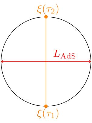
(a)

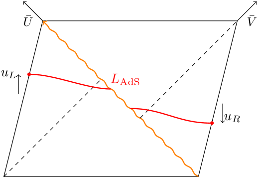
(b)

Figure 6: Shockwave geometry in (a) Euclidean signature, where we prepare the state at $t_{L}=t_{R}=-t_{\rm sw}$ by a small perturbation to the HH state using the scalar field $\xi(\tau)$ (orange), which is massless in the limit where $t_{\rm sw}\rightarrow\infty$ Shenker:2013pqa . Here $\tau_{1}=\frac{\beta(\theta)}{2}+\mathrm{i}t_{\rm sw}$, $\tau_{2}=\beta(\theta)-\tau_{1}$. (b) We display the Penrose diagram of the shockwave geometry, with the wormhole length (97) in coordinates where $\overline{U}=\arctan((x^{-})^{\Phi_{h}})$, $\overline{V}=-\arctan((x^{+})^{\Phi_{h}})$ (see e.g. Aguilar-Gutierrez:2023pnn ).

Holographic dictionary

By equating the expectation value of the chord number in the two-sided HH state (38), and the wormhole minimal geodesic length (97) in the shockwave geometry, we arrive at the following holographic dictionary

$$t_{L} =u_{L}\leavevmode\nobreak\ ,\quad t_{R}=-u_{R}\leavevmode\nobreak\ ,$$ (98a)

$$\alpha_{\rm sw} =\quantity(1-\frac{q^{\Delta}\mathrm{e}^{-\ell^{(+)}_{*}}}{\sin^{2}\theta})\mathrm{e}^{J\sin\theta t_{w}}\leavevmode\nobreak\ ,$$ (98b)

$$\Phi_{h} =2J\sin\theta\leavevmode\nobreak\ ,\quad L_{\rm reg}=\ell^{(+)}_{*}(\theta)\leavevmode\nobreak\ .$$ (98c)

where $\ell_{*}^{(+)}$ is shown in (62). While we do not need to make further approximations at this point, it is an useful consistency check to compare with the triple scaling limit previously studied in Berkooz:2022fso . In the strict shockwave limit $\alpha_{\rm sw}$ is a fixed parameter, while $t_{w}\rightarrow\infty$. This means that the term in parenthesis in (98b) must be small. This can be recovered for light operators ($\Delta\sim\mathcal{O}(1)$) when

$$\alpha_{\rm sw}\underset{\lambda\rightarrow 0}{=}\Delta_{\rm S}\frac{\lambda\leavevmode\nobreak\ \mathrm{e}^{2J\sin\theta\leavevmode\nobreak\ t_{w}}}{2\sin\theta}\quad\text{fixed}\leavevmode\nobreak\ ,$$ (99)

which is in agreement with a chord diagram calculation in the triple-scaling result considered by Berkooz:2022fso . Thus, remarkably, all the saddle point solutions of the total chord number in (38) have a geometric interpretation in the shockwave limit, which are related to spread and operator complexity in the semiclassical limit. We expect that the most general form for the semiclassical total chord number that we derived (37) for arbitrary $\theta_{L/R}\in[0,\leavevmode\nobreak\ \pi]$ still describes an AdS₂ bulk geodesic with a shockwave insertion, but it no longer describes an early perturbation of the zero chord state. The operator $\hat{\mathcal{O}}_{\Delta}$ is not necessarily a far past/future light operator, meaning that it takes the system out of equilibrium. It would be interesting to confirm our generalization from the bulk perspective by solving the corresponding dilaton gravity EOM with a shockwave insertion and two different temperatures. In terms of the original construction by Shenker:2013pqa this might be interpreted to taking the TFD out of thermal equilibrium in the early past by a heavy operator insertion; or by inserting a light operator in the later evolution.

Comparison with massive particle

Let us compare (94) with (98). When considering the shockwave as perturbations of the TFD state, we demand that $\beta_{L}=\beta_{R}$ and so we need to replace $\ell^{(-)}_{*}\rightarrow\ell^{(+)}_{*}$ in (94) (since we instead matched the bulk distance to the Krylov operator complexity of the HH state derived in (70) when $\beta_{L}=-\beta_{R}$).

Next, in the semiclassical limit for light operators, it follows from (62) that $\ell^{(+)}_{*}\rightarrow\sin^{2}\theta+2\lambda\Delta_{s}\sin\theta(1-\sin\theta)+\mathcal{O}(\lambda^{2})$. This means that to leading order (94b, 94c) can be expressed as:

$$\frac{m_{\xi}\kappa^{2}L_{b}}{\Phi_{b}} =\frac{2\pi\lambda\Delta}{\sin\theta}(1-\sin\theta)+\mathcal{O}(\lambda^{2})\leavevmode\nobreak\ ,$$ (100a)

$$L_{\rm reg} =\ell^{(+)}_{*}(\theta)+\mathcal{O}(\lambda)\leavevmode\nobreak\ .$$ (100b)

We note that the backreaction parameter (100a) is then proportional to shift parameter $\alpha_{\rm sw}$ in (99); however, they are not equal since they describe different backreaction profiles; the scalar case is a stationary matter particle according to the frames in the asymptotic boundary, while the shockwave is a massless shell inserted at $t_{w}\rightarrow\infty$.

It can be seen that (94a), (100b) (at leading order) are also consistent with $\Phi_{h}$ and $L_{\rm reg}$ in (98a) respectively. Note that the overall sign difference between the exponentially growing part of (90) and the exponentially decreasing (41). This occurs since the massive scalar is inserted at the $t=0$ slice in a HH preparation of state, instead of the shockwave perturbation which is send at $t=-t_{w}$($\rightarrow-\infty$).

4.3 From constraint quantization to the dual of the double-scaled algebra

We will discuss the canonical quantization of the bulk theory as an application of our results. So far, we have considered that the states in the chord space have conserved energy, and that the left/right sector chord numbers are integers, which implies quantization of the lengths in the bulk side according to the holographic dictionary (61). This means that the bulk is in fact a constrained system (as we expect in more general cases). For this reason, to study the quantization of the bulk theory, one must apply constraint quantization. Previous works in JT gravity and sine-dilaton gravity have been doing this even without been explicit about it Harlow:2018tqv ; Blommaert:2024whf ; Blommaert:2024ydx . The main approaches are reduced phase space quantization faddeev1969feynman , and Dirac quantization Dirac:1931kp ; dirac2013lectures ; while most other alternative approaches are closely related or equivalent to the previous ones (see e.g. Kunstatter:1990hz ).

We now look to address the main question, deriving the bulk dual of the double-scaled algebra. To achieve this, we need to find what is the bulk dual theory, and what is the corresponding holographic dual to the operators appearing in the double-scaled algebra (1). Considering a conserved energy spectrum, as we have done so far, we know that the dual theory needs to reproduce the AdS₂ geodesic lengths that we found in Sec. 4.1, 4.2. The main candidates are then JT and sine-dilaton gravity.

We will focus on canonical quantization of sine dilaton gravity with matter (instead of just JT gravity) for different reasons. As we just saw in Sec. 4.1, Krylov operator complexity with finite temperature distinguishes between physical and fake temperatures. The later being the temperature in the effective AdS₂ spacetime, which is different from the microcanonical temperature of the DSSYK model with matter. Moreover, the bulk theory needs to have a finite energy spectrum range (137). We will show that the shockwave geometry in sine-dilaton gravity indeed corresponds to the DSSYK model with a matter chord.

Now that we know what to constraint quantize, we investigate the two above mentioned methods.

Reduced phase space quantization

We want to build the Hamiltonian of the bulk theory dual to the DSSYK model starting from the lengths $\ell_{L/R}$ of the shockwave geometry in Sec. 4.2 and its canonical momenta $P_{L/R}$, since we found that the length matches the total chord number of the DSSYK model under the identification of the holographic dictionary (98).

We start imposing two pairs of constraints in the classical bulk theory. First, the ADM energy of the phase space solutions have a total ADM Hamiltonian is conserved. Its energy spectrum for the shockwave solutions with $\theta_{L}=\theta_{R}\equiv\theta$ is given by

$$H^{(\rm ADM)}_{L/R}=E_{\rm ADM}(\theta)\equiv\frac{1}{2\kappa^{2}}\cos\theta\leavevmode\nobreak\ .$$ (101)

where the overall constant matches the one of the DSSYK model (137) when

$$\frac{1}{2\kappa^{2}}=\frac{2J}{\sqrt{\lambda(1-q)}}\leavevmode\nobreak\ .$$ (102)

We proceed with the symplectic form in the covariant phase space, which is defined by,

$$\derivative{x^{a}}{t_{L/R}}=(\omega^{-1})^{ba}\partial_{b}H_{L/R}\leavevmode\nobreak\ ,\quad\text{where}\quad x^{a}=\quantity{\ell_{i},\leavevmode\nobreak\ P_{i}}\leavevmode\nobreak\ .$$ (103)

The phase space (103) can either be expressed in boundary terms, using the classical phase space solutions of (26) of the form

$$\omega=\mathrm{d}t_{L}\wedge\mathrm{d}E_{L}+\mathrm{d}t_{R}\wedge\mathrm{d}E_{R}=\frac{2J}{\sqrt{\lambda(1-q)}}\sum_{i}\mathrm{d}\ell_{i}\wedge\mathrm{d}P_{i}\leavevmode\nobreak\ ,$$ (104)

or in bulk terms, as

$$\omega=\mathrm{d}u_{L}\wedge\mathrm{d}H^{(\rm ADM)}_{L}+\mathrm{d}u_{R}\wedge\mathrm{d}H^{(\rm ADM)}_{R}=\frac{1}{2\kappa^{2}}\sum_{i}\mathrm{d}L_{\rm AdS}^{i}\wedge\mathrm{d}P_{\rm AdS}^{i}\leavevmode\nobreak\ .$$ (105)

However, as realized in Blommaert:2024whf (in a case without matter), one should impose another pair of constraints

$$P_{\rm AdS}^{L/R}\sim P_{\rm AdS}^{L/R}+2\pi\leavevmode\nobreak\ ,$$ (106)

in order to recover discrete lengths. Indeed, in the shockwave limit, where the bulk length takes the form (97), then the saddle point solutions in (29) solve the constraints (101, 106)

$${P_{\rm AdS}^{L/R}=\mathrm{i}\log(\cos\theta+\mathrm{i}\sin\theta\frac{\tanh(\delta u_{L/R})+(1-\alpha_{\rm sw})\tanh(\delta u_{R/L})}{1+(1-\alpha_{\rm sw})\tanh(\delta u_{L})\tanh(\delta u_{R})})\leavevmode\nobreak\ ,}$$

$$\mathrm{e}^{-L_{\rm AdS}^{L/R}}=\frac{2\cos P_{\rm AdS}^{L/R}-2\cos\theta+(\alpha_{\rm sw}-1)\mathrm{e}^{-L_{\rm AdS}}\mathrm{e}^{\mathrm{i}P_{\rm AdS}^{L/R}}}{\mathrm{e}^{\mathrm{i}P_{\rm AdS}^{L/R}}+(\alpha_{\rm sw}-1)\mathrm{e}^{\mathrm{i}P_{\rm AdS}^{R/L}}}\leavevmode\nobreak\ ,$$ (107a)

where we introduced the shorthand

$$\delta u_{L}=\frac{\Phi_{h}}{2}(u_{L}-u_{w})\leavevmode\nobreak\ ,\quad\delta u_{R}=-\frac{\Phi_{h}}{2}(u_{R}+u_{w})\leavevmode\nobreak\ ,$$ (108)

with $u_{w}$ being the insertion time. We can therefore use canonical phase space quantization by promoting classical variables to quantum ones

$$\quantity{L_{\rm AdS}^{L/R},\leavevmode\nobreak\ P_{\rm AdS}^{L/R}}\rightarrow\quantity{\hat{L}_{\rm AdS}^{L/R},\leavevmode\nobreak\ \hat{P}_{\rm AdS}^{L/R}}\leavevmode\nobreak\ .$$ (109)

This approach is equivalent to our path integral quantization in Sec. 2.2, the field coordinates in the gravity theory $L_{\rm AdS}^{L/R}$ are promoted to the Heisenberg operators which the gravitational path integral (dual to (24)) prepares.

We can now construct the bulk Hamiltonian at the quantum level, under the constraints (101, 106). While there is as usual the operator ambiguity in canonical quantization; we choose the following one

$$\hat{H}_{L/R}^{(\rm ADM)}=\frac{1}{\kappa^{2}}\quantity(\mathrm{e}^{-\mathrm{i}\hat{P}_{\rm AdS}^{L/R}}+\mathrm{e}^{\mathrm{i}\hat{P}_{\rm AdS}^{L/R}}\quantity(1-\mathrm{e}^{-\hat{L}_{\rm AdS}^{L/R}})+q^{\Delta}(\alpha_{\rm sw})\mathrm{e}^{\mathrm{i}\hat{P}_{\rm AdS}^{R/L}}\mathrm{e}^{-\hat{L}_{\rm AdS}^{L/R}}\quantity(1-\mathrm{e}^{-\hat{L}_{\rm AdS}^{R/L}}))\leavevmode\nobreak\ ,$$ (110)

where

$$q^{\Delta}(\alpha_{\rm sw})\equiv \frac{1}{2\alpha_{\rm sw}}\Bigg{(}\alpha_{\rm sw}(\alpha_{\rm sw}+1)+\sin^{4}\frac{\theta}{2}$$ (111)

$$+\sqrt{\frac{2}{3}}{\quantity(\sin^{2}\frac{\theta}{2}+\alpha_{\rm sw})}\sqrt{\sin^{4}\frac{\theta}{2}+\alpha_{\rm sw}(\alpha_{\rm sw}+3+\cos\theta)}\Bigg{)}\leavevmode\nobreak\ .$$

Thus, the bulk (110) and the DSSYK Hamiltonian (5) may indeed match if the holographic dictionary (98) is satisfied. Note that the operator ordering in (110) is not very important. For instance, a different natural ordering choice

$$\quantity(1-\mathrm{e}^{-\hat{L}_{\rm AdS}^{L/R}})\mathrm{e}^{\mathrm{i}\hat{P}_{\rm AdS}^{L/R}}\quad\text{instead of}\quad\leavevmode\nobreak\ \mathrm{e}^{\mathrm{i}\hat{P}_{\rm AdS}^{L/R}}\quantity(1-\mathrm{e}^{-\hat{L}_{\rm AdS}^{L/R}})$$

and similarly for the last term in (110) only amounts to an overall shift in $\hat{L}_{\rm AdS}^{L/R}$ by a factor $\lambda\mathbb{1}$.

Dirac quantization

While reduced phase-space quantization and Dirac quantization often lead to inequivalent results, once we solve the operator order ambiguity (which in this case is determined by the boundary theory), they become equivalent. Moreover, we know from Lin:2022rbf that the chord Hilbert space of the DSSYK has a bulk interpretation where the chord number is related to a geodesic length in the bulk. It then natural to examine the Dirac quantization method, since it acts directly in the Hilbert space of the theory that we seek to quantize. Based on the previous discussion, we need to implement:

$$\quantity(\hat{H}^{\rm ADM}_{L/R}-E_{\rm ADM}(\theta_{L/R}))\ket{\psi(\theta_{L},\theta_{R})} =0\leavevmode\nobreak\ ,$$ (112a)

$$\quantity(\frac{\sum_{m=-\infty}^{\infty}\mathrm{e}^{2\pi m\hat{n}_{\rm AdS}^{L/R}}}{\sum_{m=-\infty}^{\infty}1}-\mathbb{1})\ket{\psi(\theta_{L},\theta_{R})} =0\leavevmode\nobreak\ ,$$ (112b)

$\forall\ket{\psi}\in\mathcal{H}_{\rm const}$ bulk Hilbert space; where $\hat{n}_{\rm AdS}^{L/R}\equiv\hat{L}_{\rm AdS}^{L/R}/\kappa^{2}$. The last constraint is motivated by Blommaert:2024whf (requiring that the eigenvalues of the lengths $\hat{L}_{\rm AdS}^{L/R}$ are quantized). This is equivalent to imposing constraints in the chord Hilbert space of the DSSYK model from the boundary-to-bulk map in Lin:2022rbf .

In boundary terms, the Dirac constraints (112b) can be expressed as

$$(\hat{H}_{L/R}-E(\theta_{L/R}))\ket{\psi(\theta_{L},\theta_{R})}=\quantity(\frac{\sum_{m=-\infty}^{\infty}\mathrm{e}^{2\pi m\hat{n}_{L/R}}}{\sum_{m=-\infty}^{\infty}1}-\mathbb{1})\ket{\psi(\theta_{L},\theta_{R})}=0\leavevmode\nobreak\ .$$ (113)

Note that since $[\hat{H}_{L/R},\hat{n}_{L/R}]=\hat{H}_{L/R}-\frac{2J}{\sqrt{\lambda}}\hat{a}^{\dagger}_{L/R}\neq 0$, the constraints above are second class. We can solve (113) using DSSYK Hamiltonian (16) in terms of the bivariate $q^{\Delta}$-weighted q-Hermite polynomial of order $(m,\leavevmode\nobreak\ n)$ Xu:2024hoc ,

$$\bra{\Delta;n_{L},n_{R}}\ket{\psi(\theta_{L},\theta_{R})}=H_{n_{L},n_{R}}\left(\cos\theta_{L},\cos\theta_{R};q,q^{\Delta}\right)\leavevmode\nobreak\ .$$ (114)

In fact, this solves the recurrence relation

$$2xH_{n_{1},n_{2}}(x,y;q,r)=H_{n_{1}+1,n_{2}}+(1-q^{n_{1}})H_{n_{1}-1,n_{2}}+r\leavevmode\nobreak\ q^{{n_{1}}}(1-q^{n_{2}})H_{n_{1},n_{2}-1}\leavevmode\nobreak\ ,$$ (115)

$$2yH_{n_{1},n_{2}}(x,y;q,r)=H_{n_{1},n_{2}+1}+(1-q^{n_{2}})H_{n_{1},n_{2}-1}+r\leavevmode\nobreak\ q^{{n_{2}}}(1-q^{n_{1}})H_{n_{1}-1,n_{2}}\leavevmode\nobreak\ ,$$

with the initial conditions

$$H_{n_{1},0}(x,y;q,r)=H_{n_{1}}(x;q)\leavevmode\nobreak\ ,\quad H_{0,n_{2}}(x,y;q,r)=H_{n_{2}}(y;q)\leavevmode\nobreak\ .$$ (116)

On the bulk side, given that the lengths do not need to be trivially integers to satisfy (112b) in terms of $\hat{L}_{\rm AdS}^{L/R}$, we expect that the gravity side derivation of (114) for the bulk Hamiltonian (110) follows similar steps as Blommaert:2024whf . We leave it for future directions.

Bulk dual of the double-scaled algebra

Since the bulk theory is dual at the quantum level to the DSSYK model, it must have the same natural algebra of observables. However, so far we have limited our discussion to one particle irreps. What happens with arbitrary many particles? Given that the double-scaled algebra of observables acts on $\mathcal{H}_{m}$. One can suspect that, since we reproduce shockwave geometries from the boundary side (38) more particles correspond to geometry with multiple shockwaves in the AdS₂ bulk, similar to Shenker:2013yza (in the s-wave reduction). We prove this explicitly in AX .

While in the current manuscript we have only show the equality between bulk and boundary theories with one particle insertion, this remains with more particles AX . This implies that the bulk theory (sine-dilaton gravity with matter (87) for instance) with a q-deformed shockwave geometry and a bounded energy spectrum (137) satisfies the type II₁ algebra of the DSSYK model. The bulk algebra of operators dual to the double-scaled algebra (1) then corresponds to (2), which we repeat for the reader

$$\expectationvalue{\hat{H}^{(\rm ADM)}_{L/R},\leavevmode\nobreak\ \hat{\xi}^{L/R}(x)}\leavevmode\nobreak\ ,$$ (117)

where $m_{\xi}=\Delta$, and $\hat{\xi}^{L/R}(x)$ is the quantized bulk matter field in (89), where the label $L/R$ indicates the location in the two-sided AdS₂ effective geometry (82) where field is evaluated. We comment more about (2) in Sec. 5.1. Altogether, the double-scaled algebra serves as a guiding structure to derive the holographic correspondence of the DSSYK model.

4.4 Connection with the proper radial momentum

Recently, it has been argued through different examples that that the radial proper momentum of probe particles in asymptotically AdS spacetimes can be matched with spread complexity of a TFD state excited by primary CFT operator Caputa:2024sux ; Caputa:2025dep , (or for Krylov operator complexity Fan:2024iop ; see also He:2024pox ). However, the UV finiteness in holographic CFTs have not been considered in the development of the dictionary relating the proper radial momentum and Krylov complexity. Here, we take first steps in this direction in a one-dimensional model.

As mentioned in our study of the bulk description for the Krylov operator complexity (70) in Sec. 4.1 the physical temperatures on the left and right sides of Fig. 5 need to be opposite signed. For this reason, our bulk interpretation in this section is based on the effective AdS₂ geometry of sine dilaton gravity. We start from the bulk geometry (82) (with $\Phi_{h}^{L}=\Phi_{h}^{R}\equiv\Phi_{h}$) as:

$$\mathrm{d}s^{2}=\mathrm{d}\sigma^{2}-\Phi_{h}^{2}\sinh^{2}\sigma\leavevmode\nobreak\ \mathrm{d}u^{2}\leavevmode\nobreak\ ,$$ (118)

where we performed a change of variables $r=\Phi_{h}\cosh\sigma$ and gauge fixed $u_{L}=-u_{R}\equiv u$. We seek a holographic dictionary relating the black hole horizon parameter $\Phi_{h}$ in terms of DSSYK parameters $J$ and $\theta$.

We would like to describe the geodesic of a probe point particle falling from the asymptotic boundary of an AdS₂ geometry, which is determined by

$$I_{\rm point-particle}\equiv-m_{\rm particle}\int\mathrm{d}t\sqrt{\Phi_{h}^{2}\sinh^{2}\sigma(u)-\quantity(\derivative{\sigma}{u})^{2}}\leavevmode\nobreak\ .$$ (119)

One can then take a functional derivative of the above action with respect to $\sigma^{\prime}(u)$ to evaluate the proper radial momentum of the point particle; which according to its own frame (where $\sigma^{\prime}(0)=0$) is given by

$$\mathcal{P}_{\sigma}(t)=-m_{\rm particle}\cosh(\sigma_{b})\sinh(\Phi_{h}u)\leavevmode\nobreak\ .$$ (120)

where we used the geodesic solution $\coth(\sigma(u))=\coth(\sigma_{b})\cosh(\Phi_{h}u)$, with the initial location of the infalling particle $\sigma(u=0)=\sigma_{b}$ being the asymptotic boundary location. Note that, since the particle is located at the asymptotic boundary, its mass is related to the conformal dimension of a dual DSSYK operator $\hat{\mathcal{O}}_{\Delta}$ through $m_{\rm particle}=\Delta$.

Next, we compare the time dependence of the proper radial momentum (120) and the rate of growth of Krylov operator complexity (70); which is given explicitly by

$$\derivative{t}\mathcal{C}^{(\eta=-1)}(t)= \frac{2J\sin\theta}{\lambda}\frac{\quantity(\sin^{2}\theta-{\mathrm{e}^{-\ell^{(-)}_{*}(\theta)}q^{\Delta_{\rm S}}})\sinh(2J\sin\theta\leavevmode\nobreak\ t)}{\sin^{2}\theta+\quantity(\sin^{2}\theta-{\mathrm{e}^{-\ell^{(-)}_{*}(\theta)}q^{\Delta_{\rm S}}})\sinh^{2}(J\sin\theta\leavevmode\nobreak\ t)}$$ (121)

$$\simeq \frac{2J\sin\theta}{\lambda}\quantity(1-\frac{\mathrm{e}^{-\ell^{(-)}_{*}(\theta)}q^{\Delta_{\rm S}}}{\sin^{2}\theta})\sinh(2J\sin\theta\leavevmode\nobreak\ t)\leavevmode\nobreak\ ,\quad\absolutevalue{t}\ll t_{\rm max}\leavevmode\nobreak\ .$$

In the last line, we consider the early exponential growth of Krylov operator complexity below the time scale where $1+(1-{\csc^{2}\theta}\leavevmode\nobreak\ {\mathrm{e}^{-\ell^{(-)}_{*}}}q^{\Delta_{\rm S}})\sinh^{2}(2J\sin\theta\leavevmode\nobreak\ u)\approx 1$, which is given by

$$t_{\rm max}=-\frac{1}{2J\sin\theta}\log(\frac{\sin^{2}\theta-q^{\Delta_{\rm S}}\mathrm{e}^{-\ell_{*}^{(-)}}}{4\sin^{2}\theta})\leavevmode\nobreak\ .$$ (122)

Note this time scale is smaller than the scrambling time (72). Thus, we notice a relation with the proper radial momentum (120):

$$\frac{1}{J}\derivative{t}\mathcal{C}^{(\eta=-1)}(t) \simeq-\frac{\quantity(\Phi_{h}/J)}{\lambda\leavevmode\nobreak\ m_{\rm particle}\leavevmode\nobreak\ \epsilon_{\rm reg}}\quantity(1-4\frac{\mathrm{e}^{-\ell^{(-)}_{*}}q^{\Delta_{\rm S}}}{(\Phi_{h}/J)^{2}})\leavevmode\nobreak\ \mathcal{P}_{\sigma}(u)\leavevmode\nobreak\ ,\quad\absolutevalue{t}\ll t_{\rm max}\leavevmode\nobreak\ ,$$ (123a)

$$\text{provided}\quad\Phi_{h}u=2J\sin(\theta)\leavevmode\nobreak\ t\leavevmode\nobreak\ ,$$ (123b)

where we introduced a regulator $\epsilon_{\rm reg}=\sech(\sigma_{b})$ associated with the location of asymptotic boundary location $\sigma_{b}$. Note that (123b) agrees with (94) and (98c).

From (123b) we may express the constant $\ell_{*}^{(-)}$ (68) entirely in terms of the parameters $\Phi_{h}/J$, and $q^{\Delta_{\rm S}}$. Moreover, one can also express the right hand side of (123b) purely in bulk terms by (i) identifying $\lambda\equiv\absolutevalue{\log q}=8\pi G_{N}$ as in e.g. sine dilaton gravity Blommaert:2024ydx , (ii) expressing the conformal dimension $\Delta_{S}$ in terms of the mass $m_{\xi}$ (89) of the dual minimally coupled scalar field in the AdS₂ black hole, and (iii) rescaling $J$ in the time variable $t$ and of $\Phi_{h}$. Thus, we confirm that the proposal in Caputa:2024sux has a realization in the DSSYK model, at least below the time scale (122). We comment on related future directions in Sec. 5.1

On the other hand, the spread complexity of the two-sided HH state (63) does not display the transition to exponential growth and thus it cannot be matched unless one considers only the parabolic growth regime. This is in contrast with the CFT₂ case considered in Caputa:2024sux . They showed that the spread complexity of states of the form $\hat{\mathcal{O}}_{\Delta}\ket{\rm TFD}$, with $\hat{\mathcal{O}}_{\Delta}$ being a primary CFT₂ operator, does indeed display exponential growth that can be matched with proper radial momentum.

Relation with operator size

As initially defined in the finite $N$ SYK model, operator size measures the length of the operator string of a given orthonormal operator basis. It was shown in Lin:2022rbf that the operator size in the DSSYK model is related to the total chord number through

$${\rm Size}=\frac{1}{p}\quantity(\expectationvalue{\hat{N}}+\Delta_{\rm S})\leavevmode\nobreak\ ,$$ (124)

where $p$ is the number of all-to-all interactions in the SYK Hamiltonian (130) and the expectation value depend on the state under consideration. On the other hand, Krylov operator complexity corresponds to the expectation value (with respect to the two-sided HH state (7)) of the total chord number in the semiclassical limit, in (29a). Thus, they are related to the radial proper momentum of a probe particle in an AdS₂ geometry as

$$\derivative{{\leavevmode\nobreak\ \rm Size}}{t}=\frac{1}{p}\derivative{t}\mathcal{C}^{(\eta=-1)}(t)\propto\mathcal{P}_{\sigma}\leavevmode\nobreak\ .$$ (125)

The specific proportionality factor appears in (123a). On the other hand, the relation between operator size, radial momentum, and Krylov complexity growth in the SYK model and JT gravity was also explored by Jian:2020qpp . In contrast to (125), Jian:2020qpp found (in particular examples) that operator size is proportional to the proper radial momentum of a probe particle in AdS₂ space. It is curious that the relation between the proper momentum, operator size and Krylov complexity is modified in the DSSYK model in contrast to the finite N SYK Jian:2020qpp .

5 Discussion

Summary

In this work, we have derived the holographic dictionary of the DSSYK model with a one particle insertion and the bulk dual to the double-scaled algebra. We have studied general properties and observables in the two-sided HH state of the DSSYK model with matter chords (7, to elucidate the bulk description of its double-scaled algebra of observables. In the semiclassical limit, we found that there are three type of approaches to recover the same dual bulk minimal geodesic length. The Euclidean path integral of the DSSYK allowed us to prepare the HH state, and to derive the classical phase space of the DSSYK model. This method is very convenient to derive two-sided two-point correlation functions by solving EOM, and without taking a triple-scaling limit. Meanwhile, the chord diagrams allowed our derivation of the semiclassical thermodynamics of the one-particle DSSYK, and to verify our path integral results on the two-sided two-point functions with a light and a heavy operators in App. E. At last the Krylov complexity for states and operators plays a central role in deriving the holographic dictionary of the DSSYK model, and it allows for a boundary interpretation of the results closely related to quantum chaos, as discussed in Sec. 3.2. To derive it, we formulated a Lanczos algorithm (50) that evaluates Krylov operator and spread complexity simultaneously (which depends on the relative time orientation of the two-sided Hamiltonian evolution) and including finite temperature effects. This version of the Lanczos algorithm is also valid for generic two-sided Hamiltonian systems with/without a bounded spectrum. The Krylov operator and spread complexity in the two-sided HH state correspond to geodesic lengths anchored to the asymptotic boundaries with different relative boundary time orientations. We showed that the generating function of Krylov complexity is a two-sided two-point function. An interesting special case is when the boundary times evolve as $t_{L}=-t_{R}$. In this case, we observed a transition from exponential to linear growth in Krylov operator complexity; exponential decrease to a power law decay in an OTOC (resulting from the two-sided two-point correlation). We found that the scrambling time of Krylov operator complexity corresponds to that of the OTOC, and to the one in a shockwave geometry, all at finite temperature. The explicit OTOC obeys bounds found in the literature Milekhin:2024vbb . It also features submaximal chaos, and its scrambling time is independent of the system size, which is associated to hyperfast growth Susskind:2021dfc .

As for the bulk description, we showed that the backreaction of a massive particle at rest in AdS₂, or by a shockwave profile can be matched to the saddle point solutions of the total chord number evaluated in the two-sided HH state. This allowed us to derive the holographic dictionary in both cases, and then canonically quantize the bulk theory with matter (sine-dilaton gravity) to formulate the holographic dual of the double-scaled algebra. Thus, our results suggest that these three techniques take a significant role in understanding holography in the DSSYK model; and particularly, on the dynamics of its bulk dual in the presence of matter fields. For the convenience of the reader, we collected the main outcomes of the paper in App. B.

5.1 Outlook

Besides the points below, additional future directions can be found in footnotes 11, 33, 34, 19, and 29.

A bulk description of the double-scaled algebra

To formulate (2), we had to derive the holographic dictionary of the DSSYK and sine dilaton gravity (Tab. 1), and quantize the bulk theory to show that it is equivalent to the boundary one. One might try to study (2) independently of the boundary theory, deduce that it is type II₁ (which in principle involves arbitrary more particle insertions). One should carefully check that it has the same properties as the double scaled algebra. Moreover, given that sine dilaton gravity has multiple black hole and cosmological horizons, it is also important to have a bulk interpretation of the generalized horizon entropy (see e.g. Chandrasekaran:2022cip ; Chandrasekaran:2022eqq ; Penington:2023dql ; Witten:2023qsv ; Witten:2025xuc ; Penington:2024sum ; Witten:2023xze ; Witten:2021unn ; DeVuyst:2024pop ; DeVuyst:2024uvd ; Jensen:2023yxy ; Faulkner:2024gst ; Kudler-Flam:2024psh ; AliAhmad:2023etg ; Kudler-Flam:2023qfl ).

From the boundary perspective, it was realized in Tang:2024xgg that there is a natural notion of entanglement entropy for the DSSYK model that reproduces some expectations for a type II₁ algebra, and the JT gravity RT surface in the triple scaling limit. However, this is not a satisfactory interpretation of the generalized entropy of the DSSYK and its dual, as there is no good understanding of the entanglement entropy for most states even in $\mathcal{H}_{0}$, and there is no holographic interpretation of the would-be generalized horizon entropy beyond the triple-scaling limit.

It would be interesting to study this in detail by constructing traces and reduced density matrices in chord space (which we associate with the bulk Hilbert space of the DSSYK Lin:2022rbf ). For instance, taking traces with respect to the zero-open chord state, $\ket{0}$, we may evaluate expectation values as

$$\expectationvalue{\hat{A}}_{\varphi}=\bra{0}\hat{\rho}_{\varphi}\hat{A}\ket{0}\leavevmode\nobreak\ ,$$ (126)

where $\hat{\rho}_{\varphi}=\hat{\varphi}^{\dagger}\varphi$ generates arbitrary states in the chord Hilbert space, e.g.

$$\ket{\tilde{\Delta};n_{0},\dots,n_{m}}=:\hat{H}^{n_{0}}\hat{\mathcal{O}}_{\Delta_{1}}:\hat{H}^{n_{1}}\dots\hat{H}^{n_{m}}\leavevmode\nobreak\ .$$ (127)

The evaluation of generalized entropy from the dual theory as

$$S_{\rm gen}=-\tr(\hat{\rho}\log\hat{\rho})\leavevmode\nobreak\ ,$$ (128)

may be performed directly with the states in energy basis, taking similar steps as Tang:2023ocr while considering more general states than in $\hat{\varphi}\ket{0}=\ket{n}$.

Lessons dS₃ holography and sine dilaton gravity

There are different proposals on dS₃ holography based on the DSSYK model which incorporate other kinds of constraints and gauge fixing conditions as in the series of works by Verlinde:2024znh ; Verlinde:2024zrh ; Narovlansky:2023lfz ; Gaiotto:2024kze ; Tietto:2025oxn , as we have commented earlier on. While our work found that the bulk dual description of the double-scaled algebra is compatible with sine-dilaton gravity, we expect that the techniques developed here can also be applied in these other settings where there are other type of constraints to reproduce the dS₃ holographic model in Narovlansky:2023lfz . We will discuss this in an upcoming work A , to provide evidence that the original model by Narovlansky:2023lfz is consistent with our study, one simply has to impose other constraints in the chord Hilbert space. Additionally, the Krylov complexity for physical states and observables in the model by Narovlansky:2023lfz have been previously studied by Aguilar-Gutierrez:2024nau . It would be worth revisiting some of these results to connect with the findings in this work.

There was also an interesting work Blommaert:2025avl on End-Of-The-World (ETW) branes, Euclidean wormholes and matrix models from sine dilaton gravity. The connection to the DSSYK model has not been addressed for the more general type of bulk Hamiltonians that they studied based on bulk arguments. Imposing physical constraints in the DSSYK model with matter chords is a promising direction, since the ETW brane is itself the worldline of a massive particle in the effective AdS₂ description, and thus it should be connected to the one-particle space. In A we will address how imposing constraints in the path integral quantization leads to their bulk model from the boundary side. The Krylov space methods in this work also play an important role, and they might allow for a boundary interpretation in terms of quantum chaos, similar to our discussion in Sec. 3.2.

Chord amplitudes

Our evaluation of the crossed four-point function (32) from phase space methods can be seen as a prediction of a chord diagram computation (Fig. 2) where a light and a composite heavy matter chord operator intercepts a light one. We evaluated the corresponding amplitude near the end of App. E. However, to obtain an explicit answer in the semiclassical limit that indeed matches our prediction for heavy-heavy-light-light operators, we need to make an ansatz relating the energy variables of the particle chords. We can take some inspiration from an analogous diagram in JT gravity Lam:2018pvp to carry out this computation. However, this results in a very similar ansatz to having only light operators in the crossed four-point function (which we discuss at the end on App. E). Thus, this does not quite work for heavy operators. We hope to find an appropriate ansatz to carry out this evaluation. An alternative to carry out these calculations is to express the diagrams in energy basis and work out the integrals numerically, as Xu:2024gfm .

It is also important to learn how to compute more general amplitudes involving several heavy or light operators (Fig. 1 (b)) where there are relative complex phases between operator insertions. We believe that a better understanding of the classical phase space methods for these more general cases would help us to derive similar predictions that can help to predict the answer for chord diagram amplitude.

Another technical point to add in our chord diagram calculations is to include quantum corrections to the semiclassical results. We discuss this next.

On the quantum bulk theory

First, we have comment on the methods of quantization. Our study of the canonical quantization allowed us to work beyond $\lambda\rightarrow 0$. We focused on reduced phase space quantization. In principle, it is more natural to study Dirac quantization, given that the bulk Hilbert space is supposed to be described by the chord Hilbert space Lin:2022rbf . This would be a useful check of the boundary-to-bulk map in Lin:2022rbf , and to confirm our arguments in a different way.

It would also be interesting to consider quantum corrections in our saddle point solutions of the path integral. The path integral offers some advantages over computing the chord diagram amplitudes with R-matrices. Not only we can skip tedious calculations by solving EOM, this technique leads to an exact semiclassical answer in the double-scaling limit, which is often limited to triple scaling in the literature. Nevertheless, an important limitation is that if we want to derive quantum corrections, we should work instead with an effective action to a given loop order, which is not well developed in this model; while loop corrections in chord diagram amplitudes are much better studied, e.g. Goel:2023svz ; Okuyama:2023bch ; Xu:2024hoc , and also from a bulk perspective in Bossi:2024ffa . A first step in this direction would be to reproduce the first order quantum corrections in the two point correlation function of the DSSYK without matter Okuyama:2023bch ; Goel:2023svz . This could help us predict quantum corrections in the wormhole distance dual to the total chord number in the DSSYK model with matter (which would no longer be related to a Krylov complexity operator). If we consider quantum corrections to the semiclassical limit, one should account for backreaction of matter effects inside the bulk. This might be interesting to connect with bulk matter contributions in the CV in JT gravity that has been previously mentioned in Carrasco:2023fcj .

Another interesting limit is $q\rightarrow 0$, where we recover a random matrix model behavior for the DSSYK model without matter. In this limit the matterless DSSYK density of states in $\mathcal{H}_{0}$ is controlled by the Wigner surmise. This might be a useful test ground to generalize in the case with matter. For instance to study the thermodynamics of the system in the quantum regime (i.e. without $\lambda\rightarrow 0$).

More on the holographic dictionary of the two-sided DSSYK Hamiltonian

It would be interesting to relate our results with other proposals of complexity. For instance, the non-perturbative overlaps in JT gravity put forward by Miyaji:2024ity ; Miyaji:2025yvm have been used to introduce generating functions of the type $q^{\Delta\hat{N}}=\mathrm{e}^{-\Delta\hat{\ell}}$. Thus, we expect that our results can be seen as a q-deformation of theirs, which in our case includes the disk and cylinder topologies. A way to connect our results would be to study higher genus amplitude contributions to the correlation function (which we will discuss in future work). One might then compare with those in Miyaji:2024ity ; Miyaji:2025yvm in the low-energy limit. It would also be fascinating to see what aspects of the fake disk (introduced by Lin:2023trc in the semiclassical limit of the one-particle chord algebra) are captured in the semiclassical wormhole lengths (29a). For instance, the difference between physical and fake temperature in the DSSYK model was associated with a geometric description in sine dilaton gravity by Blommaert:2024ydx , which appears to be captured by the exponential growth of Krylov operator complexity below the scrambling time (71b).

Rate of growth of Krylov complexity vs the wormhole distance

We would like to interpret our results from Sec. 4 which seems to relate the growth of a wormhole geodesic length with the proper momentum of a point particle in the geometry. Both quantities are related to Krylov operator complexity (and its rate of growth) provided (123a). We would like to find a purely bulk derivation confirming this relation between seemly unrelated dynamical parameters. We also remark that we could only match the early time behavior of the rate of growth of Krylov operator complexity with the radial proper momentum (123a). It might be interesting to explore if the match can be extended to the late time regime where the Krylov operator complexity grows linearly instead.

Non-composite operators, multiple shockwaves and the switchback effect

We refer the reader to AX .

Appendix A Notation

• $J$ (130), $N$, and $p$ (131): coupling constant in the DSSYK Hamiltonian; total number of fermions; and number of all-to-all interactions, respectively.

• $\lambda=2N/p^{2}\equiv-\log q$ (131): Ratio related to the penalty factor for DSSYK Hamiltonian interceptions $q=\mathrm{e}^{-\lambda}\in[0,1]$.

• $[n]_{q}=\frac{1-q^{n}}{1-q}$: q-deformed integer.

• $(a;q)_{n}=\prod_{k=0}^{n-1}(1-aq^{k})$ (140): q-Pochhammer symbol.

• $(a_{1},a_{2},\dots a_{m};q)_{n}=\prod_{i=1}^{N}(a_{i};\leavevmode\nobreak\ q)_{n}$ (141).

• $\hat{n}$ (135): chord number operator in the zero-particle sector $\mathcal{H}_{0}$.

• $\ket{0}$: Tracial state of the DSSYK model.

• $\hat{n}_{i}^{>}=\sum_{j={i+1}}^{m}\quantity(\hat{n}_{j}+\Delta_{j})$ and $\hat{n}_{i}^{<}=\sum_{j=0}^{i-1}\quantity(\hat{n}_{j}+\Delta_{j+1})$ in (5). Similarly for $\hat{\ell^{>}}_{i}=\lambda\hat{\ell^{>}}_{i}$, and $\hat{\ell^{<}}_{i}=\lambda\hat{\ell^{<}}_{i}$.

• $Z(\beta)=\bra{0}\mathrm{e}^{-\beta\hat{H}}\ket{0}$ (145): Partition function for the DSSYK Hamiltonian $\hat{H}$ (133) without matter.

• $E(\theta)=\frac{2J\leavevmode\nobreak\ \cos(\theta)}{\sqrt{\lambda(1-q)}}$ (137): Energy spectrum of the DSSYK model.

• $S(\theta)$ (148): Thermodynamic entropy.

• $\beta$: Inverse temperature, which is given by (148) in the microcanonical ensemble.

• $\beta_{\rm fake}=\frac{4\pi}{\sin\theta}$ (78): Fake temperature.

• $H_{n}(x|q)$ (142): q-Hermite polynomials.

• $\mathrm{d}\mu(\theta)$ (143): Integration measure in the energy parametrization basis $\theta$.

• $G^{(\Delta)}(\tau)$ (150): Thermal two-point correlation function/Krylov generating function in $\mathcal{H}_{0}$.

• $\hat{\mathcal{O}}_{\Delta}$ (150): Matter chord operator with conformal dimension $\Delta$.

• $\hat{\mathcal{O}}_{\Delta}(t)\equiv\mathrm{e}^{-\mathrm{i}t\hat{H}}\hat{\mathcal{O}}_{\Delta}\mathrm{e}^{\mathrm{i}t\hat{H}}$.

• $\mathcal{H}_{m}$ (152): $m$-particle chord space.

• $\hat{N}$ (154): Total chord number with one or more particle chords.

• $\ket{\tilde{\Delta};0,\dots,0}\equiv\hat{\mathcal{O}}_{\Delta_{1}}\dots\hat{\mathcal{O}}_{\Delta_{m}}\ket{0}$, where $\tilde{\Delta}=\quantity{\Delta_{1},\dots,\Delta_{m}}$ is a collective index.

• $\chi_{k,m_{L},m_{R}}$ (10): Clebsch-Gordan coefficients.

• $E_{L/R}$ (28): Energy spectrum of the left/right sectors in $\mathcal{H}_{m}$.

• $Z_{\tilde{\Delta}}(\beta_{L},\beta_{R})$ (8): Partition function in the two-sided HH state.

• $C_{\Delta}$ (189): Heat capacity in the DSSYK model (at fixed $\lambda$, $J$, and $\Delta$).

• $G^{(\Delta_{w})}_{\tilde{\Delta}}(\tau_{L},\tau_{R})$ (58): Thermal two-point correlation function in chord matter space, corresponding to a four-point function in $\mathcal{H}_{0}\otimes\mathcal{H}_{0}$.

• $\ket{\Psi_{\tilde{\Delta}}(\tau_{L},\tau_{R})}$ (7): Double-scaled PETS, a generalization of the HH state with matter chord insertions, and complex times $\tau_{L/R}=\frac{\beta_{L/R}}{2}+\mathrm{i}t_{L/R}$.

• $\hat{\mathcal{L}}_{\eta}=\hat{H}_{R}+\eta\hat{H}_{L}$ (50): Liouvillian operator.

• $\eta=\tau_{L}/\tau_{R}$: Ratio between the two-side complex time variables, which we take to be constant in order to use the Lanczos algorithm (50). $\eta=-1$ corresponds to Krylov operator complexity for $\mathcal{O}_{\Delta}$, and $\eta=1$ to spread complexity of

• $\mathcal{C}^{(\eta)}$: Krylov complexity for two-sided Hamiltonian systems (52) that evaluates state ($\eta=+1$) (165), and operators ($\eta=-1$) (176) complexity.

• $a^{(\eta)}_{n}$ and $b^{(\eta)}_{n}$ (50): Lanczos coefficients.

• $\ket{K_{n}^{(\eta)}}$ (55): Krylov basis in the Lanczos algorithm (248).

• $\Psi_{n}^{(\eta)}(\tau)=\bra{K_{n}^{(\eta)}}\ket{\Psi_{\tilde{\Delta}}(\tau_{L}=\eta\tau,\tau_{R}=\tau)}$ (49): Amplitudes solving the Lanczos algorithm (51).

• $\hat{a}^{\dagger}_{i}$ and $\hat{\alpha}_{i}$ (14): Non-Hermitian conjugate creation and annihilation operators in $\mathcal{H}_{m}$.

• $\hat{\ell}(t_{L},t_{R})$ (26), $\hat{P}_{0/m}$ (26): Canonical distance and momenta in $\mathcal{H}_{m}$, with a two-sided Hamiltonian $\hat{H}_{L/R}$ (16a, 16b). The corresponding quantities without hat ${\ell}(t_{L},t_{R})$ (26) and ${P}_{0/m}$ (26) indicate classical variables.

• ${\Delta}_{\rm S}=\sum_{i=1}^{m}\Delta_{i}$: Sum of conformal dimensions for operators $\hat{\mathcal{O}}_{\Delta_{1}},\dots\hat{\mathcal{O}}_{\Delta_{m}}$.

• $\ell_{*}$ (27): Initial condition in the semiclassical wormhole distance, determined by the operator dimension and the energy spectrum of the system (61).

• $\ell_{*}^{(+)}$ (61), $\ell_{*}^{(-)}$ (68): Initial values Krylov operator and spread complexity (at finite temperature) respectively.

• $\gamma_{L/R}=J\sin\theta_{L/R}$ (30): frequency parameters in classical phase space solutions.

• $I_{\rm JT}[g,\Phi]$ (85), $I_{\rm SDG}[g,\Phi]$ (88), $I_{\rm(n)mc-scalar}[g,\xi,\Phi]$ (86): JT gravity, sine dilaton gravity and (non-)minimally coupled scalar field ($\xi$) actions respectively.

• $\kappa^{2}=8\pi G_{N}$ (85): Gravitational coupling.

• $\mathrm{d}s^{2}_{\rm eff}$ (82): Effective AdS₂ geometry in sine dilaton gravity.

• $L_{\rm AdS}(u_{L},u_{R})$ (97): Geodesic distance in an AdS₂ black hole background with a minimally coupled scalar field. The asymptotic boundaries are located at $r=\Phi_{b}$ and boundary times $u_{L}$ and $u_{R}$, in the coordinates (82).

• $t_{\rm sc}$ (72), $u_{\rm sc}$ (91): Scrambling time in the boundary and bulk theory respectively.

• $H_{L/R}^{(\rm ADM)}$ (105): two-sided ADM Hamiltonian.

• $\omega$: Symplectic form in the boundary (104), and in the bulk (105).

• $\hat{\mathcal{F}}$ (194): Isometric map $\mathcal{H}_{1}\rightarrow\mathcal{H}_{0}\otimes\mathcal{H}_{0}$.

• $\hat{a}_{L}=\hat{a}\otimes\mathbb{1}$, $\hat{a}_{R}=\mathbb{1}\otimes\hat{a}$: Creation and annihilation operators in $\mathcal{H}_{1}$.

• $|m,n)\equiv\ket{m}\otimes\ket{n}$; $|\theta_{1},\theta_{2})\equiv\ket{\theta_{1}}\otimes\ket{\theta_{2}}$

• $\gamma^{(q)}_{\Delta}(\theta_{L},\theta_{R})$ (202): factor in crossed four-point function amplitude (201).

• $R_{\theta_{2}\theta_{4}}^{(q)}\begin{pmatrix}\theta_{1}&\Delta_{1}\\ \theta_{2}&\Delta_{2}\end{pmatrix}$ (203): R-matrix in the crossed four-point function amplitude (201).

• ${}_{8}W_{7}(a_{1};a_{4},\ldots,a_{r+1};q,z)$ is a very-well-poised basic hypergeometric series (200).

Acronyms

• ADM: Arnowitt–Deser–Misner

• (A)dS: (Anti-)de Sitter

• CA: Complexity equals action

• CFT: Conformal field theory

• CV: Complexity equals volume

• (DS)SYK: (Double-scaled) Sachdev–Ye–Kitaev

• EOM: Equations of motion

• ETW: End-Of-The-World

• GFF: Generalized free fields

• HH: Hartle-Hawking

• Irrep: Irreducible representation

• JT: Jackiw–Teitelboim

• OTOC: Out-of-time-ordered correlator

• PETS: Partially entangled thermal state

• QRF: Quantum reference frame

• TFD: Thermofield double state

• UOGH: Universal operator growth hypothesis

• WDW: Wheeler-DeWitt

Appendix B List of the main results

We refer the reader to App. (A) (or the main text) for details about the notation used below.

DSSYK model with $m$-particles in canonical variables (16)

$$\tfrac{\sqrt{\lambda(1-q)}}{J}\hat{H}_{L}=\mathrm{e}^{-\mathrm{i}\hat{P}_{0}}+\sum_{i=0}^{m}\mathrm{e}^{\mathrm{i}\hat{P}_{i}}(1-\mathrm{e}^{-\hat{\ell}_{i}})\mathrm{e}^{-\hat{\ell}_{i}^{<}}\quad\text{where}\quad\hat{\ell}_{i}^{<}=\sum_{j=0}^{i-1}\quantity(\hat{\ell}_{j}+\lambda\Delta_{j+1})\leavevmode\nobreak\ ,$$

$$\tfrac{\sqrt{\lambda(1-q)}}{J}\hat{H}_{R}=\mathrm{e}^{-\mathrm{i}\hat{P}_{m}}+\sum_{i=0}^{m}\mathrm{e}^{\mathrm{i}\hat{P}_{i}}(1-\mathrm{e}^{-\hat{\ell}_{i}})\mathrm{e}^{-\hat{\ell}_{i}^{>}}\quad\text{where}\quad\hat{\ell}_{i}^{>}=\sum_{j={i+1}}^{m}\quantity(\hat{\ell}_{j}+\lambda\Delta_{j})\leavevmode\nobreak\ .$$

Two-sided HH state (7)

$$\ket{\Psi_{\tilde{\Delta}}(\tau_{L},\tau_{R})}=\mathrm{e}^{-\tau_{L}\hat{H}_{L}-\tau_{R}\hat{H}_{R}}\prod_{i=1}^{m}\hat{\mathcal{O}}_{\Delta_{i}}\ket{0}=\mathrm{e}^{-\tau_{L}\hat{H}_{L}-\tau_{R}\hat{H}_{R}}\ket{\Delta_{\rm S};0,0}\leavevmode\nobreak\ ,$$

where $\Delta_{\rm S}\equiv\sum_{i}\Delta_{i}$.

Partition function (8)

$$Z_{\tilde{\Delta}}(\beta_{L},\beta_{R})=\bra{\Delta_{\rm S};0,0}\mathrm{e}^{-\beta_{L}\hat{H}_{L}-\beta_{R}\hat{H}_{R}}\ket{\Delta_{\rm S};0,0}\leavevmode\nobreak\ .$$

The one-loop corrected thermodynamics of the (thermally) stable saddle point solutions for both light and heavy particles (187, 188, 189) (with $n=0$) correspond to

$$S(\theta_{L/R})\underset{\lambda\rightarrow 0}{=}-\frac{2}{\lambda}\quantity(\theta_{L/R}-\frac{\pi}{2})^{2}\leavevmode\nobreak\ ,\quad\beta_{L/R}\underset{\lambda\rightarrow 0}{=}\partialderivative{S(\theta_{L/R})}{E_{L/R}}\frac{2\theta_{L/R}-\pi}{J\sin\theta_{L/R}}\leavevmode\nobreak\ ,$$

$$C_{\Delta_{\rm S}}(\theta_{L/R})=-\beta_{L/R}^{2}\partialderivative{E_{L/R}}{\beta_{L/R}}\underset{\lambda\rightarrow 0}{=}\frac{J^{2}}{\lambda}\frac{\beta_{L/R}^{2}\sin^{2}\theta_{L/R}}{1+\quantity(\quantity(\frac{1}{2})\pi-\theta_{L/R})\cot\theta_{L/R}}\leavevmode\nobreak\ .$$

Euclidean path integral of the DSSYK ((24))

$$\int\prod_{i=0}^{m}[\mathrm{d}\ell_{i}][\mathrm{d}P_{i}]\exp\quantity[\int\mathrm{d}\tau_{L}\mathrm{d}\tau_{R}\quantity(\frac{\mathrm{i}}{\lambda}\sum_{i=0}^{m}\quantity(P_{i}(\partial_{\tau_{L}}+\partial_{\tau_{R}})\ell_{i})+H_{L}+H_{R})]\leavevmode\nobreak\ .$$

The saddle point solutions for $\ell(t_{L}=t_{R}=0)=\ell_{*}$ and $\evaluated{\partial_{t_{L/R}}\ell}_{t_{L}=t_{R}=0}=0$ are (29)

$$\ell=2\log\quantity(\cosh(\gamma_{L}t_{L})\cosh(\gamma_{R}t_{R})+\frac{J^{2}q^{\Delta_{\rm S}}\mathrm{e}^{-\ell_{*}}}{\gamma_{L}\gamma_{R}}\sinh(\gamma_{L}t_{L})\sinh(\gamma_{R}t_{R}))+\ell_{*}\leavevmode\nobreak\ ,$$

$$P_{0}=\mathrm{i}\log(\cos\theta_{L}+\mathrm{i}\sin\theta_{L}\frac{\mathrm{e}^{\ell_{*}}\sin\theta_{L}\sin\theta_{R}\tanh(\gamma_{L}t_{L})+q^{\Delta_{\rm S}}\tanh(\gamma_{R}t_{R})}{\mathrm{e}^{\ell_{*}}\sin\theta_{L}\sin\theta_{R}+q^{{\Delta_{\rm S}}}\tanh(\gamma_{R}t_{R})\tanh(\gamma_{L}t_{L})})\leavevmode\nobreak\ ,$$

$$P_{m}=\mathrm{i}\log(\cos\theta_{R}+\mathrm{i}\sin\theta_{R}\frac{\mathrm{e}^{\ell_{*}}\sin\theta_{L}\sin\theta_{R}\tanh(\gamma_{R}t_{R})+q^{\Delta_{\rm S}}\tanh(\gamma_{L}t_{L})}{\mathrm{e}^{\ell_{*}}\sin\theta_{L}\sin\theta_{R}+q^{{\Delta_{\rm S}}}\tanh(\gamma_{R}t_{R})\tanh(\gamma_{L}t_{L})})\leavevmode\nobreak\ .$$

where $\gamma_{L/R}\equiv J\sin\theta_{L/R}$. Here $\ell_{*}$ is determined by energy conservation (31):

$$\mathrm{e}^{-\ell_{*}(\theta_{L},\theta_{R})}=\frac{q^{-2\Delta_{\rm S}}}{2}\biggl{(}1+q^{2\Delta_{\rm S}}-2q^{\Delta_{\rm S}}\cos\theta_{L}\cos\theta_{R}$$

$$-\sqrt{1+q^{4\Delta_{\rm S}}+2q^{2\Delta_{\rm S}}(1+\cos(2\theta_{L})+\cos(2\theta_{R}))-4q^{\Delta_{\rm S}}(1+q^{2\Delta_{\rm S}})\cos\theta_{L}\cos\theta_{R}}\biggr{)}\leavevmode\nobreak\ .$$

We also denote

$$\ell_{*}^{+}(\theta)\equiv\ell_{*}(\theta_{L}=\theta,\theta_{R}=\theta)\leavevmode\nobreak\ ,\quad\ell_{*}^{-}(\theta)\equiv\ell_{*}(\theta_{L}=\pi-\theta,\theta_{R}=\theta)$$

Two-sided two-point correlation function (32)

$$G^{(\Delta_{w})}_{\tilde{\Delta}}(\tau_{L},\tau_{R})\equiv\frac{\bra{\Psi_{\tilde{\Delta}}(\tau_{L},\tau_{R})}q^{\Delta_{w}\hat{N}}\ket{\Psi_{\tilde{\Delta}}(\tau_{L},\tau_{R})}}{Z_{\tilde{\Delta}}(\beta_{L},\beta_{R})}$$

$$\underset{\lambda\rightarrow 0}{=}\quantity(\frac{\mathrm{e}^{-\ell_{*}/2}}{\cosh(\gamma_{L}t_{L})\cosh(\gamma_{R}t_{R})+\frac{J^{2}\mathrm{e}^{-\ell_{*}}q^{{\Delta_{\rm S}}}}{\gamma_{L}\gamma_{R}}\sinh(\gamma_{L}t_{L})\sinh(\gamma_{R}t_{R})})^{2\Delta_{w}}\leavevmode\nobreak\ .$$

Double-scaled precursors (34)

These are operators in the Schrödinger picture

$$\hat{\mathcal{O}}^{L}_{\Delta}(t_{w})\equiv\mathrm{e}^{\mathrm{i}t_{w}\hat{H}_{L}}\hat{\mathcal{O}}^{L}_{\Delta}\mathrm{e}^{-\mathrm{i}t_{w}\hat{H}_{L}}\leavevmode\nobreak\ ,\quad\hat{\mathcal{O}}^{R}_{\Delta}(t_{w})\equiv\mathrm{e}^{-\mathrm{i}t_{w}\hat{H}_{R}}\hat{\mathcal{O}}^{R}_{\Delta}\mathrm{e}^{\mathrm{i}t_{w}\hat{H}_{R}}\leavevmode\nobreak\ ,$$

where $t_{w}\in\mathbb{R}$ is the insertion time. When $t_{w}\gg\absolutevalue{t_{L/R}}$, $\theta_{=}\theta_{R}=\theta$, the saddle point solution for the rescaled total chord number is (38)

$$\ell(t_{L},t_{R})\simeq 2\log\biggl(\cosh(J\sin\theta(t_{L}+t_{R}))+\quantity(\frac{1}{4}-\frac{q^{\Delta_{\rm S}}\mathrm{e}^{-\ell_{*}^{+}(\theta)}}{4\sin^{2}\theta})\mathrm{e}^{-J\sin\theta(t_{L}-t_{R}-2t_{w})}\biggr{missing})+\ell^{(+)}_{*}(\theta)\leavevmode\nobreak\ .$$

Lanczos algorithm (50) for the two-sided DSSYK

Consider a reference state

$$\ket{\Psi_{\tilde{\Delta}}(\tau_{L}=\eta\tau,\tau_{R}=\tau)}=\mathrm{e}^{-\mathcal{L}_{\eta}\tau}\ket{\Delta_{\rm S};0,0}=\sum_{n}\Psi_{n}^{(\eta)}(\tau)\ket{K^{(\eta)}_{n}}\leavevmode\nobreak\ ,$$ (129)

where $\hat{\mathcal{L}}_{\eta}=\hat{H}_{R}+\eta\hat{H}_{L}$ is the generalized Liouvillian operator (considering $\eta=\pm 1$), and the Krylov basis $\quantity{\ket{K_{n}^{(\eta)}}}$ obeys a Lanczos algorithm

$$\hat{\mathcal{L}}_{\eta}\ket{K^{(\eta)}_{n}}=b^{(\eta)}_{n+1}\ket{K_{n+1}^{(\eta)}}+b^{(\eta)}_{n}\ket{K_{n-1}^{(\eta)}}\leavevmode\nobreak\ ,$$

where (55) gives

$$\ket{K^{(\eta)}_{n}}=c^{(\eta)}_{n}\sum_{l=0}^{n}\eta^{k}\begin{pmatrix}n\\ l\end{pmatrix}\ket{\Delta_{\rm S};l,n-l}+\text{subleading}\leavevmode\nobreak\ ,$$

with $c^{(\eta)}_{n}=\sqrt{\frac{\lambda^{n}(1-q)^{n}(1+\eta)}{2^{n}(q^{1/2};q^{1/2})_{n}(-\eta;q^{1/2})_{n+1}}}$, and the norm of other terms vanishes as $\lambda\rightarrow 0$ when $\eta=\pm$. The Lanczos coefficients (248) are

$$b^{(\eta)}_{n}\underset{\lambda\rightarrow 0}{=}\frac{2J}{\sqrt{\lambda(1-q)}}\sqrt{(1-q^{n/2})(1+\eta q^{n/2+\Delta_{\rm S}})}\leavevmode\nobreak\ .$$

Krylov operator ($\eta=-1$) and spread ($\eta=+1$) complexity correspond to (70) and (63) (from (29a)) respectively

$$\mathcal{C}^{(\eta=\pm 1)}(t)\underset{\lambda\rightarrow 0}{=}\frac{2}{\lambda}\log(A(\theta,\pm q^{\Delta_{\rm S}})+B(\theta,\pm q^{\Delta_{\rm S}})\cosh(2J\sin\theta t))\leavevmode\nobreak\ ,$$

$$A(\theta,q^{\Delta})=\frac{(\cos\theta-\cos 2\theta)q^{\Delta}+\left(1-q^{\Delta}\right)\left(q^{\Delta}+\sqrt{q^{2\Delta}-2\cos\theta q^{\Delta}+1}-1\right)}{2\sin^{2}\theta\left(q^{\Delta}+\sqrt{q^{2\Delta}-2\cos\theta q^{\Delta}+1}-1\right)}\leavevmode\nobreak\ ,$$

$$B(\theta,q^{\Delta})=\frac{q^{2\Delta}-\left((\cos\theta+\cos 2\theta)q^{\Delta}\right)-\left(1-q^{\Delta}\right)\sqrt{q^{2\Delta}-2\cos\theta q^{\Delta}+1}+1}{2\sin^{2}\theta\left(q^{\Delta}+\sqrt{q^{2\Delta}-2\cos\theta q^{\Delta}+1}-1\right)}\leavevmode\nobreak\ .$$

The $\eta=-1$ case has an associated scrambling time (72),

$$t_{\rm sc}=\frac{1}{2J\sin\theta}\log\frac{4\sin^{2}\theta q^{\Delta_{\rm S}}-\left(q^{\Delta_{\rm S}}-\sqrt{q^{2\Delta_{\rm S}}+2\cos\theta q^{\Delta_{\rm S}}+1}+1\right)^{2}}{2\left(4\sin^{2}\theta q^{\Delta_{\rm S}}+\left(q^{\Delta_{\rm S}}-\sqrt{q^{2\Delta_{\rm S}}+2\cos\theta q^{\Delta_{\rm S}}+1}+1\right)^{2}\right)}\leavevmode\nobreak\ .$$

Holographic dictionary

The reader is referred to Tab. 1 for a brief summary.

Constraint quantization

We imposed as constraints in the classical bulk theory (101, 106)

$$H^{(\rm ADM)}_{L/R}=E_{\rm ADM}(\theta_{L/R})\equiv\frac{1}{2\kappa^{2}}\cos\theta_{L/R}\leavevmode\nobreak\ ,$$

$$P_{\rm AdS}^{L/R}\sim P_{\rm AdS}^{L/R}+2\pi\leavevmode\nobreak\ .$$

The solutions of the constraints take the form

$${P_{\rm AdS}^{L/R}=\mathrm{i}\log(\cos\theta+\mathrm{i}\sin\theta\frac{\tanh(\delta u_{L/R})+(1-\alpha_{\rm sw})\tanh(\delta u_{R/L})}{1+(1-\alpha_{\rm sw})\tanh(\delta u_{L})\tanh(\delta u_{R})})\leavevmode\nobreak\ ,}$$

$$\mathrm{e}^{-L_{\rm AdS}^{L/R}}=\frac{2\cos P_{\rm AdS}^{L/R}-2\cos\theta+(\alpha_{\rm sw}-1)\mathrm{e}^{-L_{\rm AdS}}\mathrm{e}^{\mathrm{i}P_{\rm AdS}^{L/R}}}{\mathrm{e}^{\mathrm{i}P_{\rm AdS}^{L/R}}+(\alpha_{\rm sw}-1)\mathrm{e}^{\mathrm{i}P_{\rm AdS}^{R/L}}}\leavevmode\nobreak\ ,$$

with $\delta u_{L}=\frac{\Phi_{h}}{2}(u_{L}-u_{w})\leavevmode\nobreak\ ,\quad\delta u_{R}=-\frac{\Phi_{h}}{2}(u_{R}+u_{w})$. The reduced phase space quantization leads to the bulk theory (110)

$$\hat{H}_{L/R}^{(\rm ADM)}=\frac{1}{\kappa^{2}}\quantity(\mathrm{e}^{-\mathrm{i}\hat{P}_{\rm AdS}^{L/R}}+\mathrm{e}^{\mathrm{i}\hat{P}_{\rm AdS}^{L/R}}\quantity(1-\mathrm{e}^{-\hat{L}_{\rm AdS}^{L/R}})+q^{\Delta}(\alpha_{\rm sw})\mathrm{e}^{\mathrm{i}\hat{P}_{\rm AdS}^{R/L}}\mathrm{e}^{-\hat{L}_{\rm AdS}^{L/R}}\quantity(1-\mathrm{e}^{-\hat{L}_{\rm AdS}^{R/L}}))\leavevmode\nobreak\ ,$$

where

$$q^{\Delta}(\alpha_{\rm sw})\equiv\tfrac{1}{2\alpha_{\rm sw}}\Bigg{(}\alpha_{\rm sw}(\alpha_{\rm sw}+1)+\sin^{4}\tfrac{\theta}{2}+\sqrt{\tfrac{2}{3}}{\quantity(\sin^{2}\tfrac{\theta}{2}+\alpha_{\rm sw})}\sqrt{\sin^{4}\tfrac{\theta}{2}+\alpha_{\rm sw}(\alpha_{\rm sw}+3+\cos\theta)}\Bigg{)}\leavevmode\nobreak\ .$$

Given the exact correspondence between the bulk and boundary sides, we use the holographic dictionary (98) to formulate the bulk dual of the double-scaled algebra (1) as

$$\expectationvalue{\hat{H}^{(\rm ADM)}_{L/R},\leavevmode\nobreak\ \hat{\xi}^{L/R}}\leavevmode\nobreak\ .$$

Appendix C Background material

In this appendix, we briefly review general results on the DSSYK model (C.1) and Krylov complexity for operators and states (C.2) which we use throughout the manuscript. This is not intended to be a pedagogical review. The reader can find excellent reviews on the DSSYK model Berkooz:2024lgq and Krylov complexity in Baiguera:2025dkc ; Nandy:2024htc . Other useful references with some review material can be found in Lin:2022rbf ; Rabinovici:2023yex ; Verlinde:2024znh ; Aguilar-Gutierrez:2024yzu , besides the original works on DSSYK amplitudes Berkooz:2018jqr ; Berkooz:2018qkz .

C.1 Review of the DSSYK model

DSSYK model without matter chords

The SYK model (see Sachdev:1992fk ; kitaevTalks ; Cotler:2016fpe ; Maldacena:2016upp ; Saad:2018bqo ; Maldacena:2018lmt ; Jensen:2016pah ; Polchinski:2016xgd ; Chowdhury:2021qpy among many others) consists on $N$ Majorana fermions in $(0+1)$-dimensions, and $p$-body all-to-all interactions,

$$\hat{H}_{\rm SYK}=\mathrm{i}^{p/2}\sum_{I}J_{I}\hat{\psi}_{I}\leavevmode\nobreak\ ,\quad J_{I}=0\leavevmode\nobreak\ ,\quad\expectationvalue{J_{I}J_{I^{\prime}}}=\begin{pmatrix}N\\ p\end{pmatrix}^{-1}\frac{J^{2}N}{2p^{2}}\delta_{II^{\prime}}\leavevmode\nobreak\ ,$$ (130)

where $I=i_{1},\dots,\leavevmode\nobreak\ i_{p}$ is a collective index, $1\leq i_{1}<\dots<i_{p}\leq N$; $J_{I}=J_{i_{1}\dots i_{p}}$ are Gaussian distributed coupling constants; and $\hat{\psi}_{I}\equiv\hat{\psi}_{i_{1}}\dots\hat{\psi}_{i_{p}}$ is a string of Majorana fermions. They obey a Clifford algebra $\quantity{\hat{\psi}_{i},\leavevmode\nobreak\ \hat{\psi}_{j}}=2\delta_{ij}\mathbbm{1}$. We define the double-scaling limit as

$$N,\leavevmode\nobreak\ p\rightarrow\infty\leavevmode\nobreak\ ,\quad q=\mathrm{e}^{-\lambda}\leavevmode\nobreak\ ,\quad\lambda\equiv\frac{2p^{2}}{N}\leavevmode\nobreak\ \text{fixed}\leavevmode\nobreak\ .$$ (131)

The DSSYK model (and other models in the same universality class Erdos:2014zgc ; Berkooz:2024lgq ; Parisi_1994 ; Berkooz:2024evs ; Berkooz:2024ofm ; Almheiri:2024xtw ; Gao:2024lem ) becomes solvable through combinatorial methods Berkooz:2020fvm ; Berkooz:2018jqr ; Berkooz:2018qkz , even away of the low energy regime. The ensemble-averaged description of (130) can be formulated in an auxiliary (H-chord) Hilbert space

$$\mathcal{H}=\bigoplus_{n=0}^{\infty}\mathbb{C}\ket{n}\leavevmode\nobreak\ ,$$ (132)

where $n$ denotes the number of open chords at a given time slice in the chord diagram. We pick an orthonormal chord number basis $\quantity{\ket{n}}$, where the Hamiltonian in the ensemble theory is given by Berkooz:2018jqr ; Berkooz:2018qkz

$$\hat{H}=\frac{J}{\sqrt{\lambda}}\quantity(\hat{a}^{\dagger}+\hat{a})\leavevmode\nobreak\ ,$$ (133)

$$\hat{a}^{\dagger}\ket{n}=\sqrt{[n+1]_{q}}\ket{n+1}\leavevmode\nobreak\ ,\quad\hat{a}^{\dagger}\ket{n}=\sqrt{[n]_{q}}\ket{n-1}\leavevmode\nobreak\ ,$$ (134)

where $[n]_{q}\equiv\frac{1-q^{n}}{1-q}$, $\hat{a}^{\dagger}$ and $\hat{a}$ are the creation and annihilation operators of a q-deformed harmonic oscillator. We may also make a redefinition $\hat{a}^{\dagger}=\sqrt{[n]_{q}}\mathrm{e}^{-\mathrm{i}\hat{p}}$, and $\hat{a}=\mathrm{e}^{\mathrm{i}\hat{p}}\sqrt{[n]_{q}}$ to formulate the theory in terms of the chord number operator $\hat{n}$ and its conjugate momentum, $\hat{p}$:

$$\hat{n}\ket{n}=n\ket{n}\leavevmode\nobreak\ ,\quad\mathrm{e}^{\pm\mathrm{i}\hat{p}}\ket{n}=\ket{n\mp 1}\leavevmode\nobreak\ .$$ (135)

The commutation relations become:

$$\quantity[\hat{n},\leavevmode\nobreak\ \mathrm{e}^{\pm\mathrm{i}\hat{p}}]=\mp\mathrm{e}^{\pm\mathrm{i}\hat{p}}\leavevmode\nobreak\ .$$ (136)

It can be seen eigenvalues of the Hamiltonian have the following form

$$\hat{H}\ket{\theta}=E(\theta)\ket{\theta}\leavevmode\nobreak\ ,\quad E(\theta)=\frac{2J}{\sqrt{\lambda(1-q)}}{\cos\theta}\leavevmode\nobreak\ .$$ (137)

The solutions to the eigenvalue problem are

$$E(\theta)\bra{\theta}\ket{n}=\frac{J}{\sqrt{\lambda}}\quantity(\sqrt{[n]_{q}}\bra{\theta}\ket{n-1}+\sqrt{[n+1]_{q}}\bra{\theta}\ket{n+1})\leavevmode\nobreak\ .$$ (138)

with $\bra{\theta}\ket{0}=1$ are given by

$$\bra{\theta}\ket{n}={\frac{H_{n}(\cos\theta|q)}{\sqrt{(q;q)_{n}}}}\leavevmode\nobreak\ ,$$ (139)

with $(a;\leavevmode\nobreak\ q)_{n}$ is the q-Pochhammer symbol and related product:

$$(a;\leavevmode\nobreak\ q)_{n}\equiv\prod_{k=0}^{n-1}(1-aq^{k})\leavevmode\nobreak\ ,$$ (140)

$$(a_{0},\dots,a_{N};q)_{n}=\prod_{i=1}^{N}(a_{i};\leavevmode\nobreak\ q)_{n}\leavevmode\nobreak\ .$$ (141)

Meanwhile, $H_{n}(x|q)$ is the q-Hermite polynomial:

$$H_{n}(\cos\theta|q)=\sum_{k=0}^{n}\begin{bmatrix}n\\ k\end{bmatrix}_{q}\mathrm{e}^{\mathrm{i}(n-2k)\theta}\leavevmode\nobreak\ ,\quad\begin{bmatrix}n\\ k\end{bmatrix}_{q}\equiv\frac{(q;\leavevmode\nobreak\ q)_{n}}{(q;\leavevmode\nobreak\ q)_{n-k}(q;\leavevmode\nobreak\ q)_{k}}\leavevmode\nobreak\ .$$ (142)

The $\ket{\theta}$ basis is normalized such that

$$\mathbb{1}=\int_{0}^{\pi}\mathrm{d}\mu(\theta)\ket{\theta}\bra{\theta}\leavevmode\nobreak\ ,\quad\mathrm{d}\mu(\theta)\equiv\frac{\mathrm{d}\theta}{2\pi}(q,\leavevmode\nobreak\ \mathrm{e}^{\pm 2\mathrm{i}\theta};q)_{\infty}\leavevmode\nobreak\ ,\quad$$ (143)

$$\text{where}\quad(x^{\pm a_{1}\pm a_{2}};q)_{n}\equiv(x^{a_{1}+a_{2}};q)_{n}(x^{-a_{1}+a_{2}};q)_{n}(x^{-a_{1}+a_{2}};q)_{n}(x^{--a_{1}-a_{2}};q)_{n}\leavevmode\nobreak\ .$$ (144)

One can then evaluate the partition function of the model as

$$Z(\beta)=\bra{0}\mathrm{e}^{-\beta\hat{H}}\ket{0}=\int\mathrm{d}\mu(\theta)\mathrm{e}^{-\beta E(\theta)}\leavevmode\nobreak\ ,$$ (145)

which in the semiclassical limit reduces to

$$Z(\beta) \underset{\lambda\rightarrow 0}{=}\int{\mathrm{d}E(\theta)}\mathrm{e}^{S(\theta)-\beta E(\theta)}\leavevmode\nobreak\ ,$$ (146)

where we have used the following approximation for (144)

$$(x;q)_{\infty} =\exp\quantity(-\frac{{\rm Li}_{2}(x)}{\lambda}+\frac{1}{2}\log(1-x)+\mathcal{O}(\lambda))\leavevmode\nobreak\ ,$$ (147)

$$(q;q)_{\infty} =\sqrt{\frac{2\pi}{\lambda}}\exp\quantity(-\frac{\pi^{2}}{6\lambda}+\mathcal{O}(\lambda))\leavevmode\nobreak\ ,$$

$${\rm Li}_{2}(z)+{\rm Li}_{2}(z^{-1})=-\frac{\pi^{2}}{6}-\frac{1}{2}\quantity(\log(-z))^{2}\leavevmode\nobreak\ .$$

with ${\rm Li}_{2}(x)$ the dilogarithm function. The thermodynamic entropy and the microcanonical temperature in (146) are:

$$S(\theta)=-\frac{2(\frac{\pi}{2}-\theta)^{2}}{\lambda}\leavevmode\nobreak\ ,\quad\beta(\theta)=\derivative{S}{E}=2\frac{\theta-\pi/2}{J\sin\theta}$$ (148)

respectively. We can also introduce matter chords operators (also called cords), which have the form:

$$\hat{\mathcal{O}}_{\Delta} =\mathrm{i}^{\frac{p^{\prime}}{2}}\sum_{I^{\prime}}M_{I^{\prime}}\psi_{I^{\prime}}\leavevmode\nobreak\ ,\quad\expectationvalue{M_{I}}=0\leavevmode\nobreak\ ,\quad\expectationvalue{M_{I}J_{I^{\prime}}}=0\leavevmode\nobreak\ ,\quad\expectationvalue{M_{I}M_{I^{\prime}}}=\begin{pmatrix}N\\ p^{\prime}\end{pmatrix}^{-1}\delta_{II^{\prime}}\leavevmode\nobreak\ .$$ (149)

Here $\Delta\equiv p^{\prime}/p$, $I^{\prime}=i_{1},\dots,i_{p^{\prime}}$; and $M_{I^{\prime}}$ are Gaussian random couplings that are independent of $J_{I}$, and we have chosen the normalization of $\expectationvalue{M_{I}M_{I^{\prime}}}$ by requiring $\expectationvalue{\tr(\hat{\mathcal{O}}_{\Delta}^{2})}_{M}=1$, following the convention in Berkooz:2018jqr ; Berkooz:2018qkz .

One can then evaluate correlation functions in the auxiliary Hilbert space as Berkooz:2018jqr ; Berkooz:2018qkz

$$\evaluated{G^{(\Delta)}(\tau)}_{\tau=\frac{\beta}{2}+\mathrm{i}t} =\frac{\bra{0}\hat{\mathcal{O}}_{\Delta}\mathrm{e}^{-\quantity(\frac{\beta}{2}-\mathrm{i}t)\hat{H}}\hat{\mathcal{O}}_{\Delta}\mathrm{e}^{-\quantity(\frac{\beta}{2}+\mathrm{i}t)\hat{H}}\ket{0}}{Z(\beta)}$$ (150)

$$=\frac{1}{Z(\beta)}\int\quantity(\prod_{j=1,\leavevmode\nobreak\ 2}\mathrm{d}\mu(\theta_{j})\mathrm{e}^{-\quantity(\frac{\beta}{2}+(-1)^{j+1}\mathrm{i}t)E(\theta_{i})})\bra{\theta_{1}}q^{\Delta\hat{n}}\ket{\theta_{2}}\leavevmode\nobreak\ ,$$

where Berkooz:2018jqr ; Goel:2023svz

$$\bra{\theta_{i}}q^{\Delta\hat{n}}\ket{\theta_{i}}=\frac{(q^{2\Delta};q)_{\infty}}{(q^{\Delta\pm\mathrm{i}\theta_{i}\pm\mathrm{i}\theta_{j}};q)_{\infty}}\leavevmode\nobreak\ .$$ (151)

Using saddle point methods, one evaluate the integral (150) as in Goel:2023svz .

On the chord space with particle insertions

As originally discussed by Lin:2022rbf , the Fock space of q-deformed harmonic oscillators (132) is modified under the addition of chord particles in the chord diagrams (e.g. Fig. 1). Once we introduce $m\in\mathbb{Z}_{\geq 0}$ number of chord particles into the chord diagrams, the new auxiliary Hilbert space takes the form Lin:2022rbf

$$\mathcal{H}_{m}=\bigoplus_{n_{0},n_{1},\cdots,n_{m}=0}^{\infty}\mathbb{C}\ket{\tilde{\Delta},n_{0},n_{1},\cdots,n_{m}}\leavevmode\nobreak\ ,$$ (152)

where the states in $\mathcal{H}_{m}$ are represented with the same notation as (3). The inner product for the Hilbert space in (152) was worked out in Lin:2023trc . To describe this system as a q-deformed harmonic oscillator, one needs to introduce creation and annihilation operators (134) acting on the different chord number sectors in (152),

$$\hat{a}^{\dagger}_{i}\ket{\tilde{\Delta};n_{0},\dots n_{i},\dots,n_{m}} =\ket{\tilde{\Delta};n_{0},\dots,n_{i}+1,\dots n_{m}}\leavevmode\nobreak\ ,$$ (153a)

$$\hat{\alpha}_{i}\ket{\tilde{\Delta};n_{0},\dots n_{i},\dots,n_{m}} =\ket{\tilde{\Delta};n_{0},\dots,n_{i}-1,\dots n_{m}}\leavevmode\nobreak\ ,$$ (153b)

We also introduce the total chord number operator,

$$\hat{N}\ket{\tilde{\Delta},n_{0},\cdots,n_{m}}=\sum_{i=0}^{m}n_{i}\ket{\tilde{\Delta},n_{0},\cdots,n_{m}}\leavevmode\nobreak\ .$$ (154)

The two-sided Hamiltonian acting on the Fock space with matter (152) takes the form (16) Lin:2022rbf

$$\hat{H}_{L/R}=\frac{J}{\sqrt{\lambda}}\quantity(\hat{a}_{L/R}+\hat{a}^{\dagger}_{L/R})\leavevmode\nobreak\ ,\quad\text{where}$$ (155)

$$\hat{a}^{\dagger}_{L}=\hat{a}^{\dagger}_{0}\leavevmode\nobreak\ ,\quad\hat{a}_{L}=\sum_{i=0}^{m}\hat{\alpha}_{i}\quantity(\frac{1-q^{\hat{n}_{i}}}{1-q})q^{\hat{n}_{i}^{<}}\leavevmode\nobreak\ ,\quad\text{with}\quad\hat{n}_{i}^{<}=\sum_{j=0}^{i-1}\quantity(\hat{n}_{j}+\Delta_{j+1})\leavevmode\nobreak\ ,$$ (156)

$$\hat{a}^{\dagger}_{R}=\hat{a}^{\dagger}_{m}\leavevmode\nobreak\ ,\quad\hat{a}_{R}=\sum_{i=0}^{m}\hat{\alpha}_{i}\quantity(\frac{1-q^{\hat{n}_{i}}}{1-q})q^{\hat{n}_{i}^{>}}\leavevmode\nobreak\ ,\quad\text{with}\quad\hat{n}_{i}^{>}=\sum_{j={i+1}}^{m}\quantity(\hat{n}_{j}+\Delta_{j})\leavevmode\nobreak\ .$$ (157)

is discussed in more detail in Sec. 2.2.

For generality, we also discuss how the operators $\hat{\mathcal{O}}_{\Delta}$ act on the Fock space (152). Since $\hat{\mathcal{O}}_{\Delta}$ can be seen as a double-scaled auxiliary Hamiltonian, (149), one can decompose it into creation an annihilation operators acting on chord matter space, i.e. $\hat{\mathcal{O}}_{\Delta}=\hat{b}_{\Delta}+\hat{b}_{\Delta}^{\dagger}$ (in a similar way as (155)), where Xu:2024hoc

$$\hat{b}_{\Delta}^{\dagger}\ket{\tilde{\Delta};n_{0},\cdots,n_{m}}=\ket{\Delta,\tilde{\Delta};0,n_{0},\cdots,n_{m}}\leavevmode\nobreak\ .$$ (158)

Meanwhile, assuming that $\Delta_{1}=\dots=\Delta_{m}=\Delta$, we also have

$$\hat{b}_{\Delta}\ket{\Delta^{(m)};n_{0},\cdots,n_{m}}=\sum_{j=1}^{m}q^{(j-1)\Delta^{2}}q^{\Delta\sum_{l<j}n_{l}}\ket{\Delta^{(m-1)};n_{0},\cdots,n_{j-2},n_{j-1}+n_{j},\cdots,n_{m}}\leavevmode\nobreak\ .$$ (159)

Here $\Delta^{(m)}$ indicates $m$ times the same $\Delta$; $q^{\Delta^{2}}$ is the penalty factor for a crossing between two matter chords, and $q^{\Delta}$ for a crossing between Hamiltonian and matter chords. If instead we considered some $\Delta_{1\leq i\leq m}$ to be different from each other, then we only need to account for the chords with the same conformal weight as $\hat{\mathcal{O}}_{\Delta}$, so that they can be annihilated by $\hat{b}_{\Delta}$.

C.2 Krylov complexity

Quantum complexity (see reviews in Chapman:2021jbh ; Chen:2021lnq ; Baiguera:2025dkc ) are among several measures quantum chaos which is expected to be one of the distinguishing features of holographic systems Hayden:2007cs ; Sekino:2008he ; Shenker:2013pqa ; Shenker:2013yza ; Maldacena:2015waa . Generically, it is expected that quantum complexity measures in holographic systems probe regions of the black hole interior that are not accessible to entanglement entropy Susskind:2014moa . This has motivated several conjectures for geometrical observables dual to quantum complexity (called holographic complexity); most commonly capturing the properties expected for circuit complexity Susskind:2014rva . This has given rise to several holographic complexity proposals, which include the CV proposal Susskind:2014rva ; Stanford:2014jda , among many others Brown:2015bva ; Brown:2015lvg ; Couch:2016exn . In fact, it has been realized that there is an infinite number of gravitational probes exhibiting the same universal behavior as circuit complexity Belin:2021bga ; Belin:2022xmt . The defining properties in holographic complexity include a late time linear growth (which is supposed to eventually saturate, and undergo a Poincare recurrence in finite dimensional systems Chapman:2021jbh ; Susskind:2014rva ), as well as the so-called switchback effect Susskind:2014rva , a decrease in the growth of complexity due to alternating thermal scale operator insertions, also called timefolds Susskind:2014rva , which translate to shockwave pulses in an alternating order in the bulk Stanford:2014jda . If the late time evolution decreases by an overall multiple of the scrambling time for the system, then a notion of quantum complexity is said to experience a switchback effect.

The ample number of bulk proposals for holographic complexity Belin:2021bga ; Belin:2022xmt ; Myers:2024vve is reminiscent of the ambiguity in defining circuit complexity. However, despite enormous progress, holographic complexity remains, arguably, not a well developed entry in the holographic dictionary, with a few exemptions Erdmenger:2024xmj ; Erdmenger:2022lov ; Rabinovici:2023yex ; Heller:2024ldz .

Arguably, the least ambiguous measure of quantum complexity is Krylov complexity. This is constructed by decomposing a state or operator in an ordered basis, called the Krylov basis, by sequential applications of a Hamiltonian or Liouvillian operator, and summing over all amplitudes resulting from this decomposition, with an appropriate weight.

Both measures have seen several applications. For instance, as originally observed in Parker:2018yvk , there is a strong connection between the late time exponential behavior of Krylov operator complexity with the chaos bound of OTOCs Maldacena:2015waa at least in several examples (while there are some limitation, e.g. Bhattacharjee:2022vlt ; Dymarsky:2021bjq ; Camargo:2022rnt ; Chapman:2024pdw ). There has also been a lot of recent interest in spread complexity (and higher moments of its generating function Camargo:2024rrj ), as it exhibits a peak value in chaotic quantum systems, and other non-integrable (except for saddle-point dominated scramblers Huh:2023jxt ) Balasubramanian:2022tpr ; Erdmenger:2023wjg ; Baggioli:2024wbz ; Jeong:2024oao ; Huh:2023jxt ; Fu:2024fdm ; Camargo:2024rrj ; Camargo:2023eev ; Balasubramanian:2024ghv ; Alishahiha:2024vbf . The evolution of spread complexity can be directly associated with the level spacing statistics Alishahiha:2024vbf . Moreover, it has been found that the time derivative of spread complexity for CFT excited states can be sharply related with the proper momentum of a point particle in asymptotically AdS spacetimes Caputa:2024sux ; Caputa:2025dep . This provides evidence that Krylov complexity is indeed an entry in the holographic dictionary, at least in specific examples.

In the case of two-sided Hamiltonians one can also derive concrete relations between Krylov operator complexity and spread complexity of an excited state; as we develop in the main text (Sec. 3.1). The reader is also referred to Sanchez-Garrido:2024pcy for a rigorous procedure to map the spread complexity of the TFD state with an operator insertion $\hat{\mathcal{O}}$ into the corresponding operator Krylov complexity of $\hat{\mathcal{O}}$, and App. F.2 in Ambrosini:2024sre for a discussion about this.

C.3 Krylov state complexity

In the original work by Balasubramanian:2022tpr , the authors showed that the basis $\quantity{\ket{B_{n}}}$ minimizing $\sum_{n}c_{n}\absolutevalue{\bra{\varphi(t)}\ket{B_{n}}}^{2}$, with $\ket{\varphi(t)}$ being a general evolving state in the Schrödinger picture, and c_n being arbitrary monotonically increasing real coefficients, is given by the Krylov basis, $\ket{K_{n}}$, defined through a Gram-Schmidt orthogonalization of $\quantity{H^{k}\ket{\phi(t=0)}}$. The formalism was later extended by Erdmenger:2023wjg , who shows that one can threat this problem following the same Lanczos algorithm (which we introduce shortly) while allowing for complex time evolution

$$-\partial_{\tau}\ket{\varphi} =\hat{H}\ket{\psi}\leavevmode\nobreak\ ,$$ (160)

$$\ket{\varphi(\tau)} =\mathrm{e}^{-\tau\hat{H}}\ket{\varphi(0)}\leavevmode\nobreak\ ,\quad\tau\in\mathbb{C}\leavevmode\nobreak\ .$$

The Lanczos algorithm, used to construct the Krylov basis, $\quantity{\ket{K_{n}}}$, is then given by

$$\ket{A_{n+1}}\equiv(\hat{H}-a_{n})\ket{K_{n}}-b_{n}\ket{K_{n-1}}\leavevmode\nobreak\ ,$$ (161)

$$\text{If }b_{n}=0\text{ stop; otherwise }\ket{K_{n}}\equiv b_{n}^{-1}\ket{A_{n}}\leavevmode\nobreak\ ,$$

which is initialized by $\ket{K_{0}}\equiv\ket{\varphi(0)}$. The Lanczos coefficients are given by

$$a_{n}\equiv\bra{K_{n}}\hat{H}\ket{K_{n}},\qquad b_{n}\equiv(\innerproduct{A_{n}}{A_{n}})^{1/2}\leavevmode\nobreak\ .$$ (162)

We can now express (160) as

$$\ket{\varphi(\tau)}=\sum^{\mathcal{K}}_{n=0}\varphi_{n}(\tau)\ket{K_{n}}\leavevmode\nobreak\ ,$$ (163)

where $\mathcal{K}$, the Krylov space dimension, is bounded by the total Hilbert space dimension. Using the Schrödinger equation (160), we can see that the Hamiltonian is tridiagonal in the Krylov basis:

$$-\partial_{\tau}\varphi_{n}(\tau)=a_{n}\varphi_{n}(\tau)+b_{n+1}\varphi_{n+1}(\tau)+b_{n}\varphi_{n-1}(\tau)\leavevmode\nobreak\ ,$$ (164)

and $\sum_{n}|\varphi_{n}(\tau)|^{2}=\bra{\varphi_{0}}\mathrm{e}^{-\beta\hat{H}}\ket{\varphi_{0}}$ is a conserved probability in real time. The spread complexity of evolving states in complex time is then defined as

$$\mathcal{C}(t)\equiv\evaluated{\frac{\bra{\varphi(\tau)}\hat{\mathcal{C}}\ket{\varphi(\tau)}}{\bra{\varphi(\tau)}\ket{\varphi(\tau)}}}_{\tau=\beta+\mathrm{i}t}=\evaluated{\frac{\sum_{n}n|\varphi_{n}(\tau)|^{2}}{\sum_{n}\absolutevalue{\varphi_{n}(\tau)}^{2}}}_{\tau=\beta+\mathrm{i}t}\leavevmode\nobreak\ ,$$ (165)

where the Krylov complexity operator is identified with

$$\hat{\mathcal{C}}=\sum_{n}n\ket{K_{n}}\bra{K_{n}}\leavevmode\nobreak\ .$$ (166)

(165) provides the average position of a particle propagating through a one-dimensional ordered lattice generated by the Krylov basis, where each step requires more applications of the Hamiltonian $\hat{H}$, which heuristically provides a measure of quantum chaos.

In particular, in the DSSYK model without matter chords, one can see from the symmetric Hamiltonian (138) that the Krylov basis for a given seed state $\ket{K_{0}}=\ket{0}$ is simply the $\ket{K_{n}}=\ket{n}$, and the Lanczos coefficients are

$$a_{n}=0\leavevmode\nobreak\ ,\quad b_{n}=\frac{J}{\sqrt{\lambda(1-q)}}\sqrt{[n]_{q}}\leavevmode\nobreak\ .$$ (167)

The spread complexity for $\mathrm{e}^{-\hat{H}\tau}\ket{0}$ in the $\lambda\rightarrow 0$ limit is then (29a) with $t_{L}=t_{R}=t/2$ and $\sum_{i}\Delta_{i}=0$ (corresponding to no particle chord since the conformal dimensions for matter chords are strictly non-negative, as seen from (149)).

For operators

We can to express the evolution of $\hat{O}$ in the Heisenberg picture in terms of a complete basis $\quantity{\ket{x_{n}}}$ in operator space as

$$|\hat{O}) \equiv\sum_{m,\,n}O_{nm}|x_{m},\leavevmode\nobreak\ x_{n})\leavevmode\nobreak\ ,$$ (168)

with $O_{nm}\equiv\bra{x_{m}}\hat{O}\ket{x_{n}}$, and $|x_{m},\leavevmode\nobreak\ x_{n})=\ket{x_{m}}\otimes\ket{x_{n}}$. To define the Hilbert space associated with these states, one needs to specify the inner product. There are different choices when considering finite temperature ensembles Parker:2018yvk ; Barbon:2019wsy ; Anegawa:2024yia , see Sanchez-Garrido:2024pcy for a comprehensive review. For instance, in the context thermal correlation functions in boundary theories, it is often convenient to use regulated thermal inner product, where Boltzmann factors are inserted between every matter operator $\hat{O}$. The so-called Wightman inner, introduced by Parker:2018yvk for Krylov operator complexity, is then given

$$(\hat{X}|\hat{Y})=\frac{1}{Z(\beta)}\Tr(\mathrm{e}^{-\frac{\beta}{2}\hat{H}}\hat{X}^{\dagger}\mathrm{e}^{-\frac{\beta}{2}\hat{H}}\hat{Y})\leavevmode\nobreak\ .$$ (169)

The Heisenberg equation can be then expressed as

$$\partial_{t}|\hat{O}(t)) =\mathrm{i}\hat{\mathcal{L}}|\hat{O}(t))\leavevmode\nobreak\ ,$$ (170)

with $\hat{\mathcal{L}}$ the Liouvillian super-operator, defined as

$$\hat{\mathcal{L}}=\quantity[\hat{H},\leavevmode\nobreak\ \cdot\leavevmode\nobreak\ ],\quad\hat{O}(t)=\mathrm{e}^{\hat{\mathrm{i}\mathcal{L}}t}\hat{O}=\mathrm{e}^{\mathrm{i}\hat{H}t}\hat{O}\mathrm{e}^{-\mathrm{i}\hat{H}t}\leavevmode\nobreak\ .$$ (171)

Note that when $\hat{H}=\hat{H}^{\dagger}$ (which we assume throughout our discussion), then the inner product (169) is equivalent to evolving the operator in complex time,

$$(\hat{X}(t_{x})|\hat{Y}(t_{y}))=Z(\beta)^{-1}\evaluated{\Tr\quantity(\mathrm{e}^{-\tau_{x}\hat{H}}\hat{X}^{\dagger}\mathrm{e}^{-\tau^{*}_{x}\hat{H}}\mathrm{e}^{-\tau_{y}^{*}\hat{H}}\hat{Y}\mathrm{e}^{-\tau_{y}\hat{H}})}_{\tau_{x/y}=\frac{\beta}{4}+\mathrm{i}t_{x/y}}\leavevmode\nobreak\ .$$ (172)

We can therefore associate this choice of inner product with complex time evolution, similar to the Schrödinger picture in (160). We would like to use the so-called Krylov basis, $\quantity{|\hat{K}_{n})}$, defined through the recursion relation

$$|\hat{A}_{n+1})=\mathcal{L}|\hat{K}_{n})-b_{n}|\hat{K}_{n-1})\leavevmode\nobreak\ ,\quad(\hat{K}_{m}|\hat{K}_{n})=\delta_{mn}\leavevmode\nobreak\ ,$$ (173)

with $|\hat{K}_{0})=|\hat{O}(t=0))$. In writing (173), we have assumed that the system is Hermitian; otherwise, we would need to determine the Lanczos coefficients $a_{n}=(\hat{K}_{n}|\mathcal{L}|\hat{K}_{n})$ Parker:2018yvk . We may then express the solution $|\hat{O}(t))$ of (170) as

$$|\hat{O}(t))=\sum_{n=0}^{\mathcal{K}-1}\mathrm{i}^{n}\tilde{\varphi}_{n}(t)\leavevmode\nobreak\ |\hat{K}_{n})\leavevmode\nobreak\ .$$ (174)

where $\mathcal{K}$ refers to the dimension of the Krylov space (i.e. the operator subspace that is spanned by $\quantity{|\hat{K}_{n})}$), and

$$\tilde{\varphi}_{n}(\tau)=(\hat{K}_{n}|\mathrm{e}^{\mathrm{i}\hat{\mathcal{L}}t}|\hat{K}_{0})=\frac{\Tr(\hat{K}_{n}\mathrm{e}^{-\tau^{*}\hat{H}}\hat{K}_{0}\mathrm{e}^{-\tau\hat{H}})}{Z(\beta)}\leavevmode\nobreak\ ,$$ (175)

where $\tau=\beta/2+\mathrm{i}t$. One can then define the Krylov complexity of $\hat{O}(t)$ Parker:2018yvk

$$\mathcal{C}(t)=\frac{(\hat{O}(t)|\hat{\mathcal{C}}|\hat{O}(t))}{(\hat{O}(t)|\hat{O}(t))}=\evaluated{\frac{\sum_{n}n\absolutevalue{\tilde{\varphi}_{n}(\tau)}^{2}}{\sum_{n}\absolutevalue{\tilde{\varphi}_{n}(\tau)}^{2}}}_{\tau=\beta/2+\mathrm{i}t}\leavevmode\nobreak\ .$$ (176)

where we have introduced the Krylov complexity operator

$$\hat{\mathcal{C}}\equiv\sum_{n}n|\hat{K}_{n})(\hat{K}_{n}|\leavevmode\nobreak\ ,$$ (177)

in a similar way as (166). Krylov complexity for operators serves as a measure of the operator growth due to Hamiltonian evolution, in the sense of representing the mean wavepacket amplitude width in the Krylov space. It has found several applications. For instance, one can gain knowledge of the OTOC Lyapunov exponent of a chaotic quantum system without having to compute it directly, as conjectured in Parker:2018yvk through several non-trivial examples. The universal operator growth hypothesis (UOGH) Parker:2018yvk states that the late-time growth of Krylov complexity contains the information of the bound on the OTOC maximal Lyapunov exponent; ${2\pi/{\beta}}$, where ${\beta}$ is the inverse temperature of the system.

Two-sided Hamiltonians

Let us now study how to generalize the arguments above when the total Hamiltonian of the system is $\hat{H}=\hat{H}_{L}\otimes\mathbb{1}+\mathbb{1}\otimes\hat{H}_{R}$, one may represent the Liovillian acting on an operator $\hat{\mathcal{O}}_{\Delta}\otimes\mathbb{1}$ perturbing the TFD state, as

$$\mathcal{L}\hat{\mathcal{O}}_{\Delta}\ket{\rm TFD}=[\hat{H}_{L},\hat{\mathcal{O}}_{\Delta}]\ket{\rm TFD}=(\hat{H}_{L}-\hat{H}_{R})\hat{\mathcal{O}}_{\Delta}\ket{\rm TFD}\leavevmode\nobreak\ ,$$ (178)

where we used the property: $(\hat{H}_{L}-\hat{H}_{R})\ket{\rm TFD}=0$. Thus, we may represent $\hat{\mathcal{L}}=\hat{H}_{L}-\hat{H}_{R}$ when analyzing the double-scaled algebra of operators, as we do in the main text.

Using the eigenstate basis of the TFD state to perform the Choi–Jamiołkowski isomorphism in (168), it can be seen that we threat Krylov operator complexity of $|\hat{\mathcal{O}}_{\Delta}(t))$ in a thermal ensemble in the same formalism for as the spread complexity (165) of the perturbed TFD state in a thermal state

$$\mathrm{e}^{-\frac{\beta_{L}}{2}\hat{H}_{L}-\frac{\beta_{R}}{2}\hat{H}_{R}}|\hat{\mathcal{O}}_{\Delta}(t)) =\mathrm{e}^{-\frac{\beta_{L}}{2}\hat{H}_{L}-\frac{\beta_{R}}{2}\hat{H}_{R}+\mathrm{i}\hat{\mathcal{L}}t}\hat{\mathcal{O}}_{\Delta}\ket{\rm TFD}$$ (179)

$$=\mathrm{e}^{-\frac{\beta_{L}}{2}\hat{H}_{L}-\frac{\beta_{R}}{2}\hat{H}_{R}+\mathrm{i}(\hat{H}_{R}-\hat{H}_{L})t}\hat{\mathcal{O}}_{\Delta}\ket{\rm TFD}\leavevmode\nobreak\ .$$

Meanwhile, the Wightman inner product (169) is not uniquely generalizable in two-sided Hamiltonian systems for a thermal ensemble where $\beta_{L}\neq\beta_{R}$. In principle, one might use other equally valid definitions as well, which are expected to provide similar dynamical behavior (e.g. Parker:2018yvk ; Sanchez-Garrido:2024pcy ) at least in the one-sided Hamiltonian systems. For these reasons, we pick a particular choice that leads to simplifications in the Lanczos algorithm (51) for technical convenience in our discussion of Sec. 2.2.

Appendix D Partition function in the two-sided Hartle-Hawking state

In this appendix we evaluate the semiclassical partition function and related thermodynamical quantities (entropy, temperature, and heat capacity in the microcanonical ensemble) by taking expectation values with respect to the two-sided HH state (7), illustrated in Fig. 1. From the partition function, we derive the thermodynamic entropy, microcanonical temperature, and heat capacity for both light (Sec. D.1), and heavy (Sec. D.2) operators. This allows us to determine the conditions for thermal stability of the saddle point solutions.

We begin deducing the form of the partition in $\mathcal{H}_{m}$:

$$Z_{\tilde{\Delta}}(\beta_{L},\beta_{R})\equiv \bra{\tilde{\Delta};0,\dots 0}\mathrm{e}^{-\beta_{L}\hat{H}_{L}-\beta_{R}\hat{H}_{R}}\ket{\tilde{\Delta};0,\dots 0}$$ (180)

$$= \bra{{\Delta_{\rm S}};0,0}\mathrm{e}^{-\beta_{L}\hat{H}_{L}-\beta_{R}\hat{H}_{R}}\ket{{\Delta_{\rm S}};0,0}$$

where we used the $\mathcal{H}_{1}$ irrep. in (10) with $\Delta_{\rm S}=\sum_{i=0}^{m}\Delta_{i}$, and $\tilde{\Delta}=\quantity{\Delta_{1},\ldots,\Delta_{m}}$.

To carry out the evaluation in (180), we start from the energy basis $\quantity{\theta_{L},\theta_{R}}$, and apply the map $\hat{\mathcal{F}}:\leavevmode\nobreak\ \mathcal{H}_{1}\rightarrow\mathcal{H}^{L}_{0}\otimes\mathcal{H}_{0}^{R}$ (194). The energy integration measure for (180) can be expressed as (see (5.13) in Xu:2024gfm )

$$Z_{\tilde{\Delta}}(\beta_{L},\beta_{R}) =\int_{\theta_{L/R}=0}^{\theta_{L/R}=\pi}\mathrm{d}\mu(\theta_{L})\mathrm{d}\mu(\theta_{R})\frac{(q^{2{\Delta_{\rm S}}};q)_{\infty}}{(q^{{\Delta_{\rm S}}}\mathrm{e}^{\mathrm{i}(\pm\theta_{L}\pm\theta_{R})};q)_{\infty}}\mathrm{e}^{-\frac{1}{2}\quantity(\beta_{L}E(\theta_{L})+\beta_{R}E(\theta_{R}))}\leavevmode\nobreak\ .$$ (181)

To evaluate the partition function (181), we distinguish between two cases.

D.1 Light particles

Let us examine the semiclassical partition function when $\Delta$ is fixed as $\lambda\rightarrow 0$. We notice that (181) can be expressed as a thermal two-point function (150) in $\mathcal{H}_{0}$, i.e.

$$Z_{\tilde{\Delta}}(\beta_{L},\beta_{R})=Z(\beta_{L}+\beta_{R})G^{(\Delta_{\rm S})}({\beta_{L}+\beta_{R}})\leavevmode\nobreak\ .$$ (182)

Thus, the evaluation of the semiclassical partition function (181) in $\mathcal{H}_{1}$ for light fields corresponds to a known result in $\mathcal{H}_{0}$ Goel:2023svz ; Blommaert:2024ydx , which takes the form

$$Z_{\tilde{\Delta}}(\beta_{L},\beta_{R})\underset{\lambda\rightarrow 0}{=}\quantity({\sin\theta})^{2\Delta_{\rm S}}\int\mathrm{d}E(\theta)\mathrm{e}^{S(\theta)-{(\beta_{L}+\beta_{R})}E(\theta)}\leavevmode\nobreak\ .$$ (183)

Noticeably, the entropy and temperature in the microcanonical ensemble are the same as (148). Moreover, the first order quantum correction to the on-shell partition function

$$\ln Z_{\tilde{\Delta}}(\beta_{L},\beta_{R})=S(\theta_{L})+S(\theta_{R})+\bra{\theta_{R}}q^{\Delta_{\rm S}\hat{N}}\ket{\theta_{L}}-\beta_{L}E_{L}-\beta_{R}E_{L}\leavevmode\nobreak\ ,$$ (184)

follow immediately from (3.9) in Goel:2023svz by replacing $\tau\rightarrow\beta_{L}$ and $\beta-\tau\rightarrow\beta_{R}$, and $\tilde{\lambda}\rightarrow\Delta_{\rm S}\lambda$.

D.2 Heavy particles

Consider now heavy operators. We evaluate the thermodynamical properties of the DSSYK model in the microcanonical ensemble and considering thermal equilibrium in the individual left and right sectors. This means that interaction terms (i.e. $\bra{\theta_{R}}q^{\Delta\hat{n}}\ket{\theta_{L}}$ in (181)) between the chord sectors do not contribute to the density of states of the individual sectors. We can then express (181) in the semiclassical limit as

$$Z_{\tilde{\Delta}}(\beta_{L},\beta_{R})= (q^{2\Delta_{\rm S}};q)_{\infty}$$ (185)

$$\int\mathrm{d}E_{L}\mathrm{d}E_{R}\mathrm{e}^{S(\theta_{L})+S(\theta_{R})+\frac{1}{\lambda}{\rm Li}_{2}\quantity(q^{\Delta_{\rm S}}\mathrm{e}^{\pm\mathrm{i}\theta_{L}\pm\mathrm{i}\theta_{R}})}\mathrm{e}^{-\frac{1}{2}\quantity(\beta_{L}E(\theta_{L})+\beta_{R}E(\theta_{R}))}\leavevmode\nobreak\ ,$$

where we introduced the notation ${\rm Li_{2}}(\mathrm{e}^{\pm x\pm y})={\rm Li_{2}}(\mathrm{e}^{x+y})+{\rm Li_{2}}(\mathrm{e}^{x-y})+{\rm Li_{2}}(\mathrm{e}^{y-x})+{\rm Li_{2}}(\mathrm{e}^{-(x+y)})$, and we expanded the exact density of states as Berkooz:2018qkz ; Berkooz:2024lgq ; Verlinde:2024znh

$$(q,\mathrm{e}^{\pm 2\mathrm{i}\theta};q)_{\infty}=2q^{-1/8}{\sin\left(\theta\right)}\sqrt{\frac{2\pi}{\lambda}}\sum_{n=-\infty}^{\infty}\left(-1\right)^{n}\mathrm{e}^{-\frac{2}{\lambda}\left(\theta+\pi\left(n-\frac{1}{2}\right)\right)^{2}}\,,$$ (186)

in (187, 188). The saddle point solutions of the partition function lead to the following thermodynamic relations

$$S(\theta_{L/R})=-\frac{2}{\lambda}\quantity(\theta_{L/R}+n\pi-\frac{\pi}{2})^{2}\leavevmode\nobreak\ ,\quad n\in\mathbb{Z}\leavevmode\nobreak\ ,$$ (187)

$$\beta_{L/R}=\partialderivative{S(\theta_{L/R})}{E_{L/R}}=\frac{2\theta_{L/R}+(2n-1)\pi}{J\sin\theta_{L/R}}\leavevmode\nobreak\ .$$ (188)

In the analogous case of $\mathcal{H}_{0}$ it has been argued by Blommaert:2024whf and Berkooz:2024ifu that the $n\geq 1$ saddles are associated with conical deficits, and they are all required to reproduce the exact DSSYK partition function at the amplitude disk level. Our observation is that the additional saddle points are thermodynamically unstable and that they also appear in $\mathcal{H}_{m\geq 0}$, as we show below.

The corresponding heat capacity at fixed $\Delta_{\rm S}$ is given by:

$$C_{\Delta_{\rm S}}(\theta_{L/R})=-\beta_{L/R}^{2}\partialderivative{E_{L/R}}{\beta_{L/R}}\underset{\lambda\rightarrow 0}{=}\frac{J^{2}}{\lambda}\frac{\beta_{L/R}^{2}\sin^{2}\theta_{L/R}}{1+\quantity(\quantity(\frac{1}{2}-n)\pi-\theta_{L/R})\cot\theta_{L/R}}\leavevmode\nobreak\ .$$ (189)

Again, this observable does not explicitly depend on the parameter $\Delta_{\rm S}$, which is contained in $\theta_{L/R}$ though (31). Moreover, one can notice from the denominator in (189) that the heat capacity remains positive for $n=0$ in the range $\theta_{L/R}\in[0,\leavevmode\nobreak\ \pi]$ (which is unchanged by an operator $\hat{\mathcal{O}}_{\Delta}$ Xu:2024hoc ). However, the denominator becomes negative for $n\geq 1$ when $\theta_{L/R}\in[0,\leavevmode\nobreak\ \pi]$. This indicates that the additional saddle points are thermodynamically unstable. Yet, since the would-be-saddle points with $n\neq 0$ add to the exact density of states (186); they should be seen as corrections to the saddle point solution for $n=0$. This is in agreement with the bulk analysis by Blommaert:2024whf , where the authors explain that one should gauge fix the shift symmetries in the putative bulk dual description of the DSSYK model, which amounts to having $\theta\in[0,\pi]$. It is interesting to note that the addition of matter is not important in this argument, as it does not modify the saddle point thermodynamics (other than having L/R saddles).

Appendix E Thermal two-sided two-point correlation function from chord diagrams

In this section, we evaluate the thermal two-point correlation function for the two-sided HH state (7). This corresponds to a crossed four-point function when we map it with the isometric map Xu:2024hoc to $\mathcal{H}^{L}_{0}\otimes\mathcal{H}_{0}^{R}$. The relevant amplitude is illustrated in Fig. 2. Moreover, this observable corresponds to the Krylov complexity moment generating function in the semiclassical limit (i.e. $\lambda\rightarrow 0$). The goal of the computation is to provide a consistency check of our answer from phase space methods in (32). So while the classical phase space answer is valid for heavy or light operators, the explicit ansatz we use to solve the amplitude assumes only light operators.

First, we derive the general form of this amplitude $\forall q\in[0,1]$, valid when the two-sided HH state (7) contains heavy particle (i.e. when $q^{\Delta_{\rm S}}$ is held fixed as $\lambda\rightarrow 0$) operators acting on the $\ket{0}$ state. Later, we will evaluate the $\lambda\rightarrow 0$ limit of the amplitude while considering light fields $\Delta\sim\mathcal{O}(1)$ to compare with the answer obtained from classical phase space methods in (32). The amplitude we calculate in this section agrees with the one we derived for two light and two heavy fields (32) in the limit where all particles are light. We hope to report progress on a more general ansatz that works for heavy-heavy-light-light amplitudes in the future. We comment about the next steps to perform the evaluation with heavy operators.

E.1 Setting up the chord amplitude

We start from the thermal two-point function (58), ${G}^{(\Delta_{w})}_{\tilde{\Delta}}({\tau_{L},\tau_{R}})=\expectationvalue{q^{\Delta_{w}\hat{N}}}/Z_{\tilde{\Delta}}(\beta_{L},\beta_{R})$, where

$$\bra{\Psi_{\tilde{\Delta}}(\tau_{L},\tau_{R})} q^{\Delta_{w}\hat{N}}\ket{{\Psi_{\tilde{\Delta}}(\tau_{L},\tau_{R})}}=$$ (190)

$$\bra{0}\mathrm{e}^{-\tau_{4}\hat{H}_{R}}\hat{\mathcal{O}}_{\Delta_{1}}\dots\hat{\mathcal{O}}_{\Delta_{m}}\mathrm{e}^{-\tau_{3}\hat{H}_{L}}q^{\Delta_{w}\hat{N}}\mathrm{e}^{-\tau_{1}\hat{H}_{L}}\hat{\mathcal{O}}_{\Delta_{m}}\dots\hat{\mathcal{O}}_{\Delta_{1}}\mathrm{e}^{-\tau_{2}\hat{H}_{R}}\ket{0}$$

$$Z_{\tilde{\Delta}}(\beta_{L},\beta_{R}) =\bra{\tilde{\Delta};0,\dots,0}\mathrm{e}^{-\beta_{L}\hat{H}_{L}-\beta_{R}\hat{H}_{R}}\ket{\tilde{\Delta};0,\dots,0}\leavevmode\nobreak\ .$$ (191)

and

$$\tau_{1}=\frac{\beta_{L}}{2}-\mathrm{i}t_{L}\leavevmode\nobreak\ ,\quad\tau_{2}=\frac{\beta_{R}}{2}-\mathrm{i}t_{R}\leavevmode\nobreak\ ,\quad\tau_{3}=\frac{\beta_{L}}{2}+\mathrm{i}t_{L}\leavevmode\nobreak\ ,\quad\tau_{4}=\frac{\beta_{R}}{2}+\mathrm{i}t_{R}\leavevmode\nobreak\ ,$$ (192)

As usual, we express the two-sided HH state (7) in terms of a $\mathcal{H}_{1}$ irrep (9),

$$\ket{\Psi_{\tilde{\Delta}}(\tau_{L},\tau_{R})}=\mathrm{e}^{-\beta_{L}\hat{H}_{L}-\beta_{R}\hat{H}_{R}}\ket{\Delta_{\rm S};0,0}\leavevmode\nobreak\ ,$$ (193)

with $\Delta_{\rm S}=\sum_{i=1}^{m}\Delta_{i}$. Consider the isometric map $\hat{\mathcal{F}}:\leavevmode\nobreak\ \mathcal{H}_{1}\rightarrow\mathcal{H}_{0}\otimes\mathcal{H}_{0}$

$$\hat{\mathcal{F}}\ket{\Delta;n_{l},n_{R}}=(q^{\Delta}\hat{a}_{L}\hat{a}_{R};q)_{\infty}|m,n)\leavevmode\nobreak\ ,$$ (194)

where $\hat{a}_{L}=\hat{a}\otimes\mathbb{1}$, and $\hat{a}_{R}=\mathbb{1}\otimes\hat{a}$ (with $\hat{a}$ being the endomorphism in $\mathcal{H}_{0}$ (134)), and $|m,n)=\ket{m}\otimes\ket{n}$. We now can express (190) (see also (B.19) and (B.22) in Xu:2024gfm )

$$\bra{\Psi_{\tilde{\Delta}}(\tau_{L},\tau_{R})}q^{\Delta_{w}\hat{N}}\ket{{\Psi_{\tilde{\Delta}}(\tau_{L},\tau_{R})}} =\int\quantity(\prod_{i=1}^{4}\mathrm{d}\mu(\theta_{i})\mathrm{e}^{-\tau_{i}E_{i}})\bra{\theta_{1}}q^{\Delta_{\rm S}}\ket{\theta_{2}}\cdot$$ (195)

$$\cdot (\theta_{1},\theta_{2}|q^{\Delta_{w}(\hat{n}_{L}+\hat{n}_{R})}\sum_{l=0}^{\infty}\frac{(q^{2\Delta_{w}};q)_{l}}{(q;q)_{l}}q^{{\Delta_{\rm S}}l}\hat{a}_{L}^{l}\hat{a}_{R}^{l}|\theta_{3},\theta_{4})\leavevmode\nobreak\ ,$$

where $\hat{n}_{L}=\hat{n}\otimes\mathbb{1}$, and $\hat{n}_{R}=\mathbb{1}\otimes\hat{n}$ with $\hat{n}$ in (135).

Moreover, we can perform the sum above from (A.7) in Okuyama:2024yya (also in szablowski2013q ):

$$(\theta_{1},\theta_{2}|q^{\Delta_{w}(\hat{n}_{L}+\hat{n}_{R})}\sum_{l=0}^{\infty}\frac{(q^{2\Delta_{w}};q)_{l}}{(q;q)_{l}}q^{{\Delta_{\rm S}}l}\hat{a}_{L}^{l}\hat{a}_{R}^{l}|\theta_{3},\theta_{4})=$$ (196)

$$\bra{\theta_{1}}q^{\Delta_{w}\hat{n}_{L}}\ket{\theta_{3}}\bra{\theta_{2}}q^{\Delta_{w}\hat{n}_{R}}\ket{\theta_{4}}\sum_{l=0}^{\infty}q^{{\Delta_{\rm S}}l}\frac{Q_{l}(\cos\theta_{1}|q^{\Delta_{w}}\mathrm{e}^{\pm\mathrm{i}\theta_{3}};q)Q_{l}(\cos\theta_{2}|q^{\Delta_{w}}\mathrm{e}^{\pm\mathrm{i}\theta_{4}};q)}{(q,q^{2\Delta_{w}};q)_{l}}\leavevmode\nobreak\ ,$$

where $Q_{l}(\cos\theta|X,Y;q)$ are the Al-Salam-Chihara polynomials al1976convolutions , which are given by

$$Q_{l}(\cos\theta|X,Y;q)=\frac{(XY;q)_{l}}{X^{l}}\sum_{n=0}^{\infty}\frac{(q^{-l},X\mathrm{e}^{\pm\mathrm{i}\theta};q)_{n}}{(XY;q)_{n}}q^{n}\leavevmode\nobreak\ ,$$ (197)

and they satisfy $Q_{-1}=0$, $Q_{0}=1$ in the recurrence relation

$$2\cos\theta\leavevmode\nobreak\ Q_{n}=Q_{n+1}+(X+Y)q^{n}Q_{n}+(1-XYq^{n-1})(1-q^{n})Q_{n-1}\leavevmode\nobreak\ .$$ (198)

It is known that the Fourier kernel of (196) can be evaluated as askey1996general (14.8):

$$\sum_{l=0}^{\infty}q^{{\Delta_{\rm S}}l}\frac{Q_{l}(\cos\theta_{1}|q^{\Delta_{w}}\mathrm{e}^{\pm\mathrm{i}\theta_{3}};q)Q_{l}(\cos\theta_{2}|q^{\Delta_{w}}\mathrm{e}^{\pm\mathrm{i}\theta_{4}};q)}{(q,q^{2\Delta_{w}};q)_{l}}$$ (199)

$$=\frac{(q^{\Delta_{\rm S}}\mathrm{e}^{-\mathrm{i}(\theta_{3}+\theta_{4})},q^{{\Delta_{\rm S}}+\Delta_{w}}\mathrm{e}^{\mathrm{i}(\theta_{4}\pm\theta_{1})},q^{{\Delta_{\rm S}}+\Delta_{w}}\mathrm{e}^{\mathrm{i}(\theta_{3}\pm\theta_{2})};q)_{\infty}}{(q^{{\Delta_{\rm S}}+\Delta_{w}}\mathrm{e}^{\mathrm{i}(\theta_{3}+\theta_{4})},q^{\Delta_{\rm S}}\mathrm{e}^{\mathrm{i}\quantity(\pm\theta_{1}\pm\theta_{2})};q)_{\infty}}\cdot$$

$$\quad\cdot{}_{8}W_{7}\quantity(q^{{\Delta_{\rm S}}+2\Delta_{w}-1}\mathrm{e}^{\mathrm{i}\quantity(\theta_{3}+\theta_{4})},q^{\Delta_{\rm S}}\mathrm{e}^{\mathrm{i}\quantity(\theta_{3}+\theta_{4})},q^{\Delta_{w}}\mathrm{e}^{\mathrm{i}\quantity(\theta_{1}\pm\theta_{3})},q\mathrm{e}^{\mathrm{i}\quantity(\theta_{4}\pm\theta_{2})};q,q^{\Delta_{\rm S}}\mathrm{e}^{-\mathrm{i}(\theta_{3}+\theta_{4})})\leavevmode\nobreak\ ,$$

where ${}_{8}W_{7}$ is a very-well-poised basic hypergeometric series

$${}_{r+1}W_{r}(a_{1};a_{4},\ldots,a_{r+1};q,z)=\sum_{j=0}^{\infty}\frac{1-a_{1}q^{2j}}{1-a_{1}}\frac{(a_{1},a_{4},\ldots,a_{r+1};q)_{j}z^{j}}{(q,qa_{1}/a_{4},\ldots,qa_{1}/a_{r+1};q)_{j}}\leavevmode\nobreak\ .$$ (200)

We can now combine (195, 196, 199, 200) with the ${}_{8}W_{7}$ integral representation in (B.23) Berkooz:2018jqr (also in gasper2011basic ). The thermal two-point correlation function (58) for the two-sided HH state (7) then takes the same form as (5.5) in Berkooz:2018jqr (i.e. a four-point function in $\mathcal{H}_{0}\otimes\mathcal{H}_{0}$ of the DSSYK model)

$${G}^{(\Delta_{w})}_{\tilde{\Delta}}({\tau_{L},\tau_{R}})=\frac{1}{Z_{\tilde{\Delta}}(\beta_{L},\beta_{R})}\int \quantity(\prod_{i=1}^{4}\mathrm{d}\mu(\theta_{i})\mathrm{e}^{-\tau_{i}E_{i}})R_{\theta_{2}\theta_{4}}^{(q)}\begin{pmatrix}\theta_{1}&{\Delta_{\rm S}}\\ \theta_{3}&\Delta_{w}\end{pmatrix}\cdot$$ (201)

$$\cdot\gamma^{(q)}_{{\Delta_{\rm S}}}(\theta_{1},\theta_{2})\gamma^{(q)}_{{\Delta_{\rm S}}}(\theta_{3},\theta_{4})\gamma^{(q)}_{\Delta_{w}}(\theta_{1},\theta_{3})\gamma^{(q)}_{\Delta_{w}}(\theta_{2},\theta_{4})\leavevmode\nobreak\ ,$$

where we introduced a shorthand $E_{i}\equiv\frac{2J}{\lambda}\cos\theta_{i}$; and we also denoted

$$\gamma^{(q)}_{\Delta}(\theta_{L},\theta_{R})\equiv\sqrt{\bra{\theta_{L}}q^{\Delta\hat{n}}\ket{\theta_{R}}}=\sqrt{\frac{(q^{2\Delta};q)_{\infty}}{(q^{\Delta}\mathrm{e}^{\pm\mathrm{i}\theta_{L}\pm\mathrm{i}\theta_{R}};q)_{\infty}}}\leavevmode\nobreak\ .$$ (202)

The R-matrix appearing in (201) is defined as Berkooz:2018jqr

$$\begin{split}&R_{\theta_{2}\theta_{4}}^{(q)}\begin{pmatrix}\theta_{1}&\Delta_{\rm S}\\ \theta_{2}&\Delta_{w}\end{pmatrix}=-\frac{1}{(q;q)_{\infty}^{3}(1-q)^{3}}\frac{\Gamma_{q}(1+\Delta_{\rm S}-\Delta_{w}+\mathrm{i}y_{1}-\mathrm{i}y_{4})\Gamma_{q}(\Delta_{w}-\Delta_{\rm S}+\mathrm{i}y_{4}-\mathrm{i}y_{1})}{\Gamma(1+\Delta_{\rm S}-\Delta_{w}+\mathrm{i}y_{1}-\mathrm{i}y_{4})\Gamma(\Delta_{w}-\Delta_{\rm S}+\mathrm{i}y_{4}-\mathrm{i}y_{1})}\cdot\\ &\cdot\sqrt{\frac{\Gamma_{q}(\Delta_{w}-\mathrm{i}y_{4}\pm\mathrm{i}y_{2})\Gamma_{q}(\Delta_{w}+\mathrm{i}y_{1}\pm\mathrm{i}y_{3})\Gamma_{q}(\Delta_{\rm S}-\mathrm{i}y_{1}\pm\mathrm{i}y_{2})\Gamma_{q}(\Delta_{\rm S}+\mathrm{i}y_{4}\pm\mathrm{i}y_{3})}{\Gamma_{q}(\Delta_{w}+\mathrm{i}y_{4}\pm\mathrm{i}y_{2})\Gamma_{q}(\Delta_{w}-\mathrm{i}y_{1}\pm\mathrm{i}y_{3})\Gamma_{q}(\Delta_{\rm S}+\mathrm{i}y_{1}\pm\mathrm{i}y_{2})\Gamma_{q}(\Delta_{\rm S}-\mathrm{i}y_{4}\pm\mathrm{i}y_{3})}}\cdot\\ &\cdot\int_{\mathcal{T}}\frac{ds}{2\pi\mathrm{i}}q^{s-\Delta_{\rm S}+\mathrm{i}y_{4}-\mathrm{i}y_{3}}\frac{\Gamma(s+1-\Delta_{\rm S}+\mathrm{i}y_{4}-\mathrm{i}y_{3})\Gamma(s+1-\Delta_{w}+\mathrm{i}y_{1}-\mathrm{i}y_{3})}{\Gamma_{q}(s+1-\Delta_{\rm S}+\mathrm{i}y_{4}-\mathrm{i}y_{3})\Gamma_{q}(s+1-\Delta_{w}+\mathrm{i}y_{1}-\mathrm{i}y_{3})}\cdot\\ &\quad\cdot\frac{\Gamma_{q}(s)\Gamma_{q}(s-2\mathrm{i}y_{3})\Gamma_{q}(s+\mathrm{i}y_{1}+\mathrm{i}y_{4}-\mathrm{i}y_{3}\pm\mathrm{i}y_{2})\Gamma(\Delta_{\rm S}-s-\mathrm{i}y_{4}+\mathrm{i}y_{3})\Gamma(\Delta_{w}-s+\mathrm{i}y_{3}-\mathrm{i}y_{1})}{\Gamma_{q}(s+\Delta_{w}+\mathrm{i}y_{1}-\mathrm{i}y_{3})\Gamma_{q}(s+\Delta_{\rm S}+\mathrm{i}y_{4}-\mathrm{i}y_{3})},\end{split}$$ (203)

where we denote $y_{i}=\quantity(\pi-\theta_{i})/\lambda$, and $\mathcal{T}$ is a contour in the complex plane passing through the imaginary axis of $s$, which can be deformed to avoid the poles of the different $\Gamma$ functions in the integrand (see Fig. 7).

E.2 Semiclassical evaluation for heavy or light operators

So far, the expressions are valid for arbitrary $q\in[0,1)$, however, we are interested in the semiclassical regime $\lambda\rightarrow 0$, and possibly in adding quantum corrections. Given that $\Delta_{w}$ in $\gamma^{(q)}_{\Delta_{w}}(\theta_{1},\theta_{3})$, $\gamma^{(q)}_{\Delta_{w}}(\theta_{2},\theta_{4})$ is a fixed number as $\lambda\rightarrow 0$, then the factors $\gamma^{(q)}_{\Delta_{w}}(\theta_{i},\theta_{j})\rightarrow\delta(\theta_{i}-\theta_{j})$ in the $\lambda\rightarrow 0$ limit. We should thus employ the following ansatz to evaluate the semiclassical limit of the amplitude (58)

$$\theta_{1}=\theta_{L}+\lambda\leavevmode\nobreak\ \alpha_{L}\leavevmode\nobreak\ ,\quad\theta_{3}=\theta_{L}-\lambda\leavevmode\nobreak\ \alpha_{L}\leavevmode\nobreak\ ,$$ (204)

$$\theta_{2}=\theta_{R}+\lambda\leavevmode\nobreak\ \alpha_{R}\leavevmode\nobreak\ ,\quad\theta_{4}=\theta_{R}-\lambda\leavevmode\nobreak\ \alpha_{R}\leavevmode\nobreak\ .$$ (205)

To leading order, the measure of integration in (201) can be then expressed

$$\prod_{i=1}^{4}\mathrm{d}\mu(\theta_{i})\underset{\lambda\rightarrow 0}{=}{16\pi^{2}}\mathrm{d}\theta_{L}\mathrm{d}\theta_{R}\mathrm{d}\alpha_{L}\mathrm{d}\alpha_{R}\mathrm{e}^{2\quantity(S(\theta_{L})+S(\theta_{R}))}(4\sin\theta_{L}\sin\theta_{R})^{2}\leavevmode\nobreak\ ,$$ (206)

where $S(\theta)=-\frac{2}{\lambda}\quantity(\theta-\frac{\pi}{2})^{2}$, and we applied the relations (147, 147). Meanwhile, the Boltzmann weight in (201) becomes

$$\mathrm{e}^{-\sum_{i=1}^{4}\tau_{i}E(\theta_{i})}=\mathrm{e}^{-\beta_{L}E(\theta_{L})-\beta_{R}E(\theta_{R})+2\sum_{i=L,R}\alpha_{i}\sin\theta_{i}(2\tau_{i}-\beta_{i})}\leavevmode\nobreak\ ,$$ (207)

where the relation between $\tau_{1\leq i\leq 4}$ with $t_{L/R}$ and $\beta_{L/R}$ is given in (192).

We move on with the product of $\gamma^{(q)}_{\Delta}$ functions (202):

$$\gamma^{(q)}_{{\Delta_{\rm S}}}(\theta_{1},\theta_{2})\gamma^{(q)}_{{\Delta_{\rm S}}}(\theta_{3},\theta_{4})\gamma^{(q)}_{\Delta_{w}}(\theta_{1},\theta_{3})\gamma^{(q)}_{\Delta_{w}}(\theta_{2},\theta_{4})$$ (208)

$$=\sqrt{\frac{(q^{2\Delta_{\rm S}};q)^{2}_{\infty}(q^{2\Delta_{w}};q)^{2}_{\infty}}{(q^{\Delta_{\rm S}\pm\mathrm{i}\alpha_{L}\pm\mathrm{i}\alpha_{R}}\mathrm{e}^{\mathrm{i}\quantity(\pm\theta_{L}\pm\theta_{R})},q^{\Delta_{w}}\mathrm{e}^{\pm 2\mathrm{i}\theta_{L}},q^{\Delta_{w}}\mathrm{e}^{\pm\mathrm{i}2\theta_{R}},q^{\Delta_{w}\pm 2\mathrm{i}\alpha_{L}},q^{\Delta_{w}\pm 2\mathrm{i}\alpha_{R}};q)_{\infty}}}$$

$$\underset{\lambda\rightarrow 0}{=}\mathcal{N}\frac{\sqrt{\Gamma(\Delta_{w}\pm 2\mathrm{i}\alpha_{L})\Gamma(\Delta_{w}\pm 2\mathrm{i}\alpha_{R})}}{\Gamma(2\Delta_{w})}(q^{2\Delta_{\rm S}};q)_{\infty}\mathrm{e}^{\frac{\pi^{2}}{6\lambda}-\frac{S(\theta_{L})+S(\theta_{R})}{2}}\quantity(4\sin(\theta_{L})\sin(\theta_{R}))^{\Delta_{w}-1/2}\cdot$$

$$\quad\cdot\mathrm{e}^{\frac{1}{2\lambda}{\rm Li}_{2}\quantity(q^{\Delta_{\rm S}}\mathrm{e}^{\mathrm{i}(\pm\theta_{L}\pm\theta_{R})})}\quantity(\quantity(1+q^{2\Delta_{\rm S}}-2\cos(\theta_{L}+\theta_{R}))\quantity(1+q^{2\Delta_{\rm S}}-2\cos(\theta_{L}-\theta_{R})))^{\Delta_{\rm S}-1/2},$$

where in the last equality we using the same notation as in (185) for ${\rm Li_{2}}(\mathrm{e}^{\pm x\pm y})$. We also applied (147), and the following expansions Blommaert:2024ydx ; Xu:2024gfm ;

$${\rm Li_{2}}(x(1-\lambda y)) ={\rm Li_{2}}(x)+\lambda y\log(1-x)+\mathcal{O}(\lambda^{2})\leavevmode\nobreak\ ,$$ (209)

$$\frac{(q^{2\Delta};q)_{\infty}}{(q^{\Delta}\mathrm{e}^{\pm\mathrm{i}\theta};q)_{\infty}} \underset{\lambda\rightarrow 0}{=}\mathcal{N}\frac{\Gamma(\Delta\pm\mathrm{i}\theta)}{\Gamma(2\Delta)}\leavevmode\nobreak\ .$$

Note that $\mathcal{N}$ is a numerical factor (i.e. independent of $\Delta$ and $\theta$).

On the other hand, the R-matrix in (58) with the Ansatz (204) at leading order becomes

$$R_{\theta_{2}\theta_{4}}^{(q)}\begin{pmatrix}\theta_{1}&\Delta_{\rm S}\\ \theta_{2}&\Delta_{w}\end{pmatrix}\underset{\lambda\rightarrow 0}{=}-\frac{1}{(q;q)_{\infty}^{3}(1-q)^{3}}\prod_{i=L,R}\sqrt{\frac{\Gamma(\Delta_{w}-2\mathrm{i}\alpha_{i})\Gamma_{q}(\Delta_{w}-\frac{2\mathrm{i}}{\lambda}\quantity(\pi-\theta_{i}))}{\Gamma(\Delta_{w}+2\mathrm{i}\alpha_{i})\Gamma_{q}(\Delta_{w}+\frac{2\mathrm{i}}{\lambda}\quantity(\pi-\theta_{i}))}}\cdot$$ (210)

$$\leavevmode\nobreak\ \cdot\sqrt{\frac{\Gamma_{q}(\Delta_{\rm S}+\frac{\mathrm{i}}{\lambda}(\theta_{L}-\theta_{R})\pm\mathrm{i}(\alpha_{L}-\alpha_{R}))\Gamma_{q}(\Delta_{\rm S}\pm\frac{\mathrm{i}}{\lambda}(2\pi-\theta_{L}-\theta_{R})+\mathrm{i}(\alpha_{L}+\alpha_{R}))}{\Gamma_{q}(\Delta_{\rm S}-\frac{\mathrm{i}}{\lambda}(\theta_{L}-\theta_{R})\pm\mathrm{i}(\alpha_{L}-\alpha_{R}))\Gamma_{q}(\Delta_{\rm S}\pm\frac{\mathrm{i}}{\lambda}(2\pi-\theta_{L}-\theta_{R})-\mathrm{i}(\alpha_{L}+\alpha_{R}))}}\cdot$$

$$\leavevmode\nobreak\ \cdot\int_{\mathcal{T}}q^{s-\Delta_{\rm S}}\mathrm{e}^{\mathrm{i}(\theta_{L}-\theta_{R})}\frac{\Gamma(-s+\Delta_{w}+2\mathrm{i}\alpha_{L})\Gamma_{q}\quantity(-s+\Delta_{\rm S}+\mathrm{i}\quantity(\alpha_{L}-\alpha_{R})-\frac{\mathrm{i}}{\lambda}\quantity(\theta_{L}-\theta_{R}))}{\Gamma(s+\Delta_{w}-2\mathrm{i}\alpha_{L})\Gamma_{q}(s+\Delta_{\rm S}-\mathrm{i}(\alpha_{L}-\alpha_{R})+\frac{\mathrm{i}}{\lambda}\quantity(\theta_{L}-\theta_{R}))}\cdot$$

$$\leavevmode\nobreak\ \cdot\leavevmode\nobreak\ \leavevmode\nobreak\ \Gamma_{q}(s)\Gamma_{q}\quantity(s-\frac{2\mathrm{i}}{\lambda}(\pi-\theta_{L})-2\mathrm{i}\alpha_{L})\Gamma_{q}\quantity(s+\frac{2\mathrm{i}}{\lambda}(\pi-\theta_{R})-2\mathrm{i}\alpha_{L})\Gamma(2\mathrm{i}(\alpha_{L}-\alpha_{R}))\leavevmode\nobreak\ ,$$

where we have not yet taken the $\lambda\rightarrow 0$ limit in the $\Gamma_{q}$ functions whose argument contains $\mathrm{i}\theta/\lambda$ terms. Before doing that, we should specify the scaling of $\Delta_{\rm S}$ as $\lambda\rightarrow 0$. We distinguish two cases:

$$\text{Heavy operators}\leavevmode\nobreak\ :\quad q^{\Delta_{\rm S}}=\mathrm{e}^{-\lambda\Delta_{\rm S}}\leavevmode\nobreak\ \text{is fixed as}\leavevmode\nobreak\ \lambda\rightarrow 0\leavevmode\nobreak\ ;$$ (211)

$$\text{Light operators}\leavevmode\nobreak\ :\quad{\Delta_{\rm S}}\leavevmode\nobreak\ \text{is fixed as}\leavevmode\nobreak\ \lambda\rightarrow 0\leavevmode\nobreak\ .$$

There are useful relations that can help us to perform the evaluation of the $\Gamma_{q}(\mathrm{i}x/\lambda+y)$ terms in (210) as $\lambda\rightarrow 0$. For instance, consider (A.5) in Mukhametzhanov:2023tcg

$$\frac{\Gamma_{q}(\frac{\mathrm{i}x}{\lambda}+y_{1})}{\Gamma_{q}(\frac{\mathrm{i}x}{\lambda}+y_{2})}\underset{\lambda\rightarrow 0}{=}\quantity(\frac{1-\mathrm{e}^{-\mathrm{i}x}}{\lambda})^{y_{1}-y_{2}}\leavevmode\nobreak\ ,$$ (212)

with $x$, $y_{1,2}$ being fixed parameters as $\lambda\rightarrow 0$. The necessary terms to simplify the ratio (212) are not present in (210). One could multiply and divide by appropriate factors like $\Gamma_{q}(\pm\mathrm{i}\frac{\theta}{\lambda})$ to get a similar expression as (212); however this produces additional terms that do not cancel out. Thus, we need an ansatz to be able to perform the full evaluation of the semiclassical R-matrix when $\hat{\mathcal{O}}_{\tilde{\Delta}}$ is a heavy composite operator. Nevertheless, we have a prediction about the exact answer we should recover, i.e. (32) (also included in App. B). In the future, we would like to find the correct ansatz for $\theta_{L/R}$ that confirms our answer from classical phase space methods (See Sec. 5.1). We will now treat the light operator case in (211), where we indeed know what the correct ansatz is. We will show how to consistently recover the expected answer in the $\lambda\rightarrow 0$ limit.

E.3 Exact evaluation for light operators

Once we let $\hat{\mathcal{O}}_{\tilde{\Delta}}$ be a single or composite light operator, the terms $\gamma^{(q)}_{\Delta_{\rm S}}(\theta_{1},\theta_{3})$, $\gamma^{(q)}_{\Delta_{\rm S}}(\theta_{2},\theta_{4})$, defined in (202), inform us that the correct implementation of the ansatz (204) in the $\lambda\rightarrow 0$ limit is

$$\theta_{1}=\theta+\lambda\quantity(\alpha_{L}+\chi)\leavevmode\nobreak\ ,\quad\theta_{3}=\theta+\lambda\quantity(\alpha_{L}-\chi)\leavevmode\nobreak\ ,$$ (213)

$$\theta_{2}=\theta+\lambda\quantity(\alpha_{R}+\chi)\leavevmode\nobreak\ ,\quad\theta_{4}=\theta+\lambda\quantity(\alpha_{R}-\chi)\leavevmode\nobreak\ ,$$ (214)

where $\theta,\leavevmode\nobreak\ \chi,\leavevmode\nobreak\ \alpha_{L/R}$ are parameters independent of $\lambda$. We can proceed as we discussed in the more general case, including the Jacobian determinant, and using the approximations (147, 147). We see that the term in the measure of integration together with the Boltzmann weight in parenthesis of (201) can be expressed as

$$\prod_{i=1}^{4}\mathrm{d}\mu(\theta_{i})\mathrm{e}^{-\tau_{i}E_{i}}= 4\pi^{2}\lambda\mathrm{d}\theta\mathrm{d}\alpha_{L}\mathrm{d}\alpha_{R}\mathrm{d}\chi\leavevmode\nobreak\ (2\sin\theta)^{4}\cdot$$ (215)

$$\cdot\mathrm{e}^{4S(\theta)-\quantity(\beta_{L}+\beta_{R})E(\theta)+2J\sin\theta\quantity(\chi(\beta_{L}-\beta_{R})+\alpha_{L}\quantity(2\tau_{L}-\beta_{L})+\alpha_{R}\quantity(2\tau_{R}-\beta_{R}))}\leavevmode\nobreak\ .$$

The (arguably) next simplest term to evaluate is the product of $\gamma^{(q)}_{\Delta}(\theta_{L},\theta_{R})$ functions in (201)

$$\gamma^{(q)}_{{\Delta_{\rm S}}}(\theta_{1},\theta_{2})\gamma^{(q)}_{{\Delta_{\rm S}}}(\theta_{3},\theta_{4})\gamma^{(q)}_{\Delta_{w}}(\theta_{1},\theta_{3})\gamma^{(q)}_{\Delta_{w}}(\theta_{2},\theta_{4})$$ (216)

$$=\sqrt{\frac{(q^{2\Delta_{\rm S}};q)^{2}_{\infty}(q^{2\Delta_{w}};q)^{2}_{\infty}}{(q^{\Delta_{\rm S}\pm\mathrm{i}(\alpha_{L}+\alpha_{R})}\mathrm{e}^{\pm 2\mathrm{i}\theta},q^{{\Delta_{\rm S}}\pm\mathrm{i}(\alpha_{L}-\alpha_{R})\pm 2\mathrm{i}\chi},q^{\Delta_{w}\pm 2\mathrm{i}\chi}\mathrm{e}^{\pm 2\mathrm{i}\theta},q^{\Delta_{w}\pm 2\mathrm{i}\alpha_{R}},q^{\Delta_{w}\pm 2\mathrm{i}\alpha_{L}};q)_{\infty}}}$$

$$\underset{\lambda\rightarrow 0}{=}\mathcal{N}(\sin\theta)^{2(\Delta_{\rm S}+\Delta_{w}-1)}\mathrm{e}^{-2S(\theta)}\tfrac{\sqrt{\Gamma(\Delta_{\rm S}\pm\mathrm{i}(\alpha_{L}-\alpha_{R})\pm 2\mathrm{i}\chi)\Gamma(\Delta_{w}\pm 2\mathrm{i}\alpha_{L})\Gamma(\Delta_{w}\pm 2\mathrm{i}\alpha_{R})}}{\Gamma(2\Delta_{\rm S})\Gamma(2\Delta_{w})}\leavevmode\nobreak\ ,$$

where we used (147, 147, 209) in the last step.

We proceed with the evaluation of the R-matrix (203) (which we simplified in (210)) using the ansatz (213). In particular, the square root term is relatively straightforward; so we will first threat the integral on the complex plane,

$$\int_{\mathcal{T}}\frac{\mathrm{d}s}{2\pi\mathrm{i}}q^{s-\Delta_{\rm S}-\mathrm{i}(\alpha_{L}-\alpha_{R}-2\chi)}\Gamma_{q}\quantity(s\pm\frac{2\mathrm{i}}{\lambda}\quantity(\pi-\theta)-2\mathrm{i}\quantity(\alpha_{L}-\chi))\Gamma(s-2\mathrm{i}\quantity(\alpha_{L}-\alpha_{R}))\cdot$$ (217)

$$\qquad\quad\cdot\Gamma(s)\frac{\Gamma(-s+\Delta_{\rm S}+\mathrm{i}\quantity(\alpha_{L}-\alpha_{R}-2\chi))\Gamma(-s+\Delta_{w}+2\mathrm{i}\alpha_{L}))}{\Gamma(s+\Delta_{w}-2\mathrm{i}\alpha_{L})\Gamma(s+\Delta_{\rm S}-\mathrm{i}\quantity(\alpha_{L}-\alpha_{R}-2\chi))}\leavevmode\nobreak\ ,$$

where $\mathcal{T}$ is a contour in the imaginary axis of $s$. We need to identifying the poles of the $\Gamma$ functions, which follow from the Weierstrass form

$$\Gamma(x)=\frac{\mathrm{e}^{-\gamma_{EM}x}}{x}\prod_{n=1}^{\infty}\quantity(\quantity(1+\frac{x}{n})^{-1}\mathrm{e}^{x/n})\leavevmode\nobreak\ ,$$ (218)

with $\gamma_{EM}$ being the Euler-Mascheroni constant; so that we only need to threat simple poles at $x=\mathbb{Z}_{\leq 0}$.

The product of $\Gamma$ functions in (217) has several poles, as illustrated in Fig. 7. The dominant ones come from

$$s=0\leavevmode\nobreak\ ,\quad s=2\mathrm{i}(\alpha_{L}-\alpha_{R})\leavevmode\nobreak\ .$$ (219)

Meanwhile the poles at $s\rightarrow\mathbb{R}\pm\mathrm{i}\infty$ (as $\lambda\rightarrow 0$), or with $n\neq 0$ in (218) are suppressed contributions since there are more $\Gamma$ terms in the numerator than in the denominator (as discussed in more detail in App. B of Mertens:2017mtv for JT gravity).

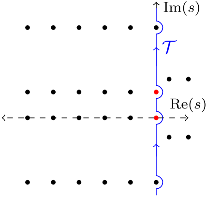
Figure 7: Illustration of the poles (red and black dots) of the Gamma functions involved in the R-matrix integral (217) in the complex plane $s$, where the dominant poles at $s=0$ and $s=i(\alpha_{R}-\alpha_{L})$ are showed in red. Figure based on Mertens:2017mtv .

Thus, we recover the total R-matrix in $\lambda\rightarrow 0$ regime as

$$R_{\theta_{2}\theta_{4}}^{(q)}\begin{pmatrix}\theta_{1}&\Delta_{\rm S}\\ \theta_{2}&\Delta_{w}\end{pmatrix}\underset{\lambda\rightarrow 0}{=}-\frac{\mathrm{e}^{\frac{\pi^{2}}{2\lambda}}}{(2\pi\lambda)^{3/2}}\sqrt{\frac{\Gamma_{q}(\Delta_{w}\pm\frac{2\mathrm{i}}{\lambda}(\pi-\theta)-2\mathrm{i}\chi)}{\Gamma_{q}(\Delta_{w}\pm\frac{2\mathrm{i}}{\lambda}(\pi-\theta)+2\mathrm{i}\chi)}\prod_{i=L,R}\frac{\Gamma(\Delta_{w}-2\mathrm{i}\alpha_{i})}{\Gamma(\Delta_{w}+2\mathrm{i}\alpha_{i})}}\cdot$$ (220)

$$\cdot\sqrt{\frac{\Gamma(\Delta_{\rm S}\pm\mathrm{i}\quantity(\alpha_{L}-\alpha_{R}+2\chi))\Gamma_{q}(\Delta_{\rm S}\pm\frac{2\mathrm{i}}{\lambda}(\pi-\theta)+\mathrm{i}(\alpha_{L}+\alpha_{R}))}{\Gamma(\Delta_{\rm S}\pm\mathrm{i}\quantity(\alpha_{L}-\alpha_{R}-2\chi))\Gamma_{q}(\Delta_{\rm S}\pm\frac{2\mathrm{i}}{\lambda}(\pi-\theta)-\mathrm{i}(\alpha_{L}+\alpha_{R}))}}\biggl{(}\Gamma\quantity(2\mathrm{i}(\alpha_{R}-\alpha_{L}))\cdot$$

$$\cdot\frac{\Gamma_{q}\quantity(\pm\frac{2\mathrm{i}}{\lambda}(\pi-\theta)-2\mathrm{i}(\alpha_{L}-\chi))\Gamma(\Delta_{\rm S}+\mathrm{i}\quantity(\alpha_{L}-\alpha_{R}-2\chi))\Gamma(\Delta_{w}+2\mathrm{i}\alpha_{L})}{\Gamma(\Delta_{\rm S}-\mathrm{i}\quantity(\alpha_{L}-\alpha_{R}-2\chi))\Gamma(\Delta_{w}-2\mathrm{i}\alpha_{L})}+\quantity(L\leftrightarrow R)\biggr{)}\leavevmode\nobreak\ .$$

Thus, combining our results thus far, the thermal correlation function can be expressed

$$\expectationvalue{q^{\Delta_{w}\hat{N}}}=-\mathcal{N}\int\mathrm{d}\theta\mathrm{d}\alpha_{L}\mathrm{d}\alpha_{R}\mathrm{d}\chi(2\sin\theta)^{2(\Delta_{\rm S}+\Delta_{w}+1)}\mathrm{e}^{2S(\theta)-(\beta_{L}+\beta_{R})E(\theta)+2J\chi\sin\theta\quantity(\beta_{L}-\beta_{R})}\cdot$$ (221)

$$\cdot\mathrm{e}^{2J\sin\theta\sum_{i=L,R}\alpha_{i}(2\tau_{i}-\beta_{i})}\quantity(\prod_{i=L,R}\Gamma(\Delta_{w}-2\mathrm{i}\alpha_{i}))\sqrt{\frac{\Gamma(\Delta_{\rm S}\pm\mathrm{i}\quantity(\alpha_{L}-\alpha_{R})\pm 2\mathrm{i}\chi)}{\Gamma(2\Delta_{w})^{2}\Gamma(2\Delta_{\rm S})^{2}}}\cdot$$

$$\cdot\sqrt{\frac{\Gamma_{q}(\Delta_{w}\pm\frac{2\mathrm{i}(\pi-\theta)}{\lambda}-2\mathrm{i}\chi)\Gamma(\Delta_{\rm S}\pm\mathrm{i}(\alpha_{L}-\alpha_{R})+2\mathrm{i}\chi)\Gamma(\Delta_{\rm S}\pm\frac{2\mathrm{i}}{\lambda}(\pi-\theta)+\mathrm{i}(\alpha_{L}+\alpha_{R}))}{\Gamma_{q}(\Delta_{w}\pm\frac{2\mathrm{i}(\pi-\theta)}{\lambda}+2\mathrm{i}\chi)\Gamma(\Delta_{\rm S}\pm\mathrm{i}(\alpha_{L}-\alpha_{R})-2\mathrm{i}\chi)\Gamma(\Delta_{\rm S}\pm\frac{2\mathrm{i}}{\lambda}(\pi-\theta)-\mathrm{i}(\alpha_{L}+\alpha_{R}))}}\cdot$$

$$\cdot\biggl{(}\frac{\Gamma\quantity(2\mathrm{i}(\alpha_{R}-\alpha_{L}))\Gamma_{q}\quantity(\pm\frac{2\mathrm{i}(\pi-\theta)}{\lambda}-2\mathrm{i}(\alpha_{L}-\chi))\Gamma(\Delta_{\rm S}+\mathrm{i}\quantity(\alpha_{L}-\alpha_{R}-2\chi))\Gamma(\Delta_{w}+2\mathrm{i}\alpha_{L})}{\Gamma(\Delta_{\rm S}-\mathrm{i}\quantity(\alpha_{L}-\alpha_{R}-2\chi))\Gamma(\Delta_{w}-2\mathrm{i}\alpha_{L})}+\quantity(L\leftrightarrow R)\biggr{)}\leavevmode\nobreak\ .$$

Since $\Gamma(2\mathrm{i}(\alpha_{L}-\alpha_{R}))$ has a simple pole when $\alpha_{L}=\alpha_{R}$ (besides the $n\neq 0$ poles in (218) which are subleading contributions in (221)), we can perform either of the $\alpha_{L}$ or $\alpha_{R}$ integrals along its real line from the residue theorem, where

$${{\rm Res}\quantity(\Gamma(2\mathrm{i}(\alpha_{R}-\alpha_{L})),\alpha_{L}=\alpha_{R})}=-4\pi\leavevmode\nobreak\ ,$$ (222)

and we relabel the remaining variable $\alpha_{R/L}\rightarrow\alpha$. Thus, (221) then transforms into

$$\expectationvalue{q^{\Delta_{w}\hat{N}}}= \mathcal{N}\int\mathrm{d}\theta\mathrm{d}\alpha\mathrm{d}\chi(2\sin\theta)^{2(\Delta_{\rm S}+\Delta_{w}+1)}\cdot$$ (223)

$$\cdot\mathrm{e}^{2S(\theta)-(\beta_{L}+\beta_{R})E(\theta)+2J\chi\sin\theta\quantity(\beta_{L}-\beta_{R})+2J\sin\theta\alpha(2(\tau_{L}+\tau_{R})-\beta_{L}-\beta_{R})}\cdot$$

$$\cdot\frac{\Gamma(\Delta_{w}\pm 2\mathrm{i}\alpha)\Gamma(\Delta_{\rm S}\pm 2\mathrm{i}\chi)}{\Gamma(2\Delta_{w})\Gamma(2\Delta_{\rm S})}\Gamma_{q}\quantity(\pm\frac{2\mathrm{i}(\pi-\theta)}{\lambda}-2\mathrm{i}(\alpha-\chi))\cdot$$

$$\cdot\sqrt{\frac{\Gamma_{q}(\Delta_{w}\pm\frac{2\mathrm{i}(\pi-\theta)}{\lambda}-2\mathrm{i}\chi)\Gamma_{q}(\Delta_{\rm S}\pm\frac{2\mathrm{i}(\pi-\theta)}{\lambda}+2\mathrm{i}\alpha)}{\Gamma_{q}(\Delta_{w}\pm\frac{2\mathrm{i}(\pi-\theta)}{\lambda}+2\mathrm{i}\chi)\Gamma_{q}(\Delta_{\rm S}\pm\frac{2\mathrm{i}(\pi-\theta)}{\lambda}-2\mathrm{i}\alpha)}}\leavevmode\nobreak\ .$$

We can significantly simplify the remaining terms using the leading order relation (212),

$$\frac{\Gamma_{q}(\Delta_{w}\pm\frac{2\mathrm{i}(\pi-\theta)}{\lambda}-2\mathrm{i}\chi)\Gamma_{q}(\Delta_{\rm S}\pm\frac{2\mathrm{i}}{\lambda}(\pi-\theta)+2\mathrm{i}\alpha)}{\Gamma_{q}(\Delta_{w}\pm\frac{2\mathrm{i}}{\lambda}(\pi-\theta)+2\mathrm{i}\chi)\Gamma_{q}(\Delta_{\rm S}\pm\frac{2\mathrm{i}}{\lambda}(\pi-\theta)-2\mathrm{i}\alpha)}\underset{\lambda\rightarrow 0}{=}\quantity(\frac{2\sin\theta}{\lambda})^{4\mathrm{i}(\gamma-\alpha)}\leavevmode\nobreak\ ,$$ (224)

$$\Gamma_{q}\quantity(\pm\frac{2\mathrm{i}(\pi-\theta)}{\lambda}-2\mathrm{i}(\alpha-\chi))=\quantity(\frac{2\sin\theta}{\lambda})^{4\mathrm{i}(\alpha-\gamma)}{\Gamma_{q}\quantity(\pm\frac{2\mathrm{i}(\pi-\theta)}{\lambda})}\leavevmode\nobreak\ ,$$

where we multiplied and divided by $\Gamma_{q}\quantity(\pm\frac{2\mathrm{i}(\pi-\theta)}{\lambda})$. Using the definition

$$\Gamma_{q}(x)\equiv(1-q)^{1-x}\frac{(q;q)_{\infty}}{(q^{x};q)_{\infty}}\leavevmode\nobreak\ ,$$ (225)

we can express

$$\Gamma_{q}\quantity(\pm\frac{2\mathrm{i}(\pi-\theta)}{\lambda})=\frac{(q;q)_{\infty}^{3}(1-q)^{2}}{(q,\mathrm{e}^{\pm 2\mathrm{i}(\pi-\theta)};q)_{\infty}}\leavevmode\nobreak\ .$$ (226)

Now, we can recognize the term in the denominator as the measure of integration in the energy basis (143) (up to a factor $2\pi$). From (147) the semiclassical limit of (226) reduces to

$$\Gamma_{q}\quantity(\pm\frac{2\mathrm{i}(\pi-\theta)}{\lambda})\underset{\lambda\rightarrow 0}{=}\frac{\pi\lambda\mathrm{e}^{-\frac{\pi^{2}}{2\lambda}-S(\theta)}}{\sin\theta}\leavevmode\nobreak\ .$$ (227)

Thus, combining all terms in (223), we get

$$\expectationvalue{q^{\Delta_{w}\hat{N}}}=\mathcal{N} \int\mathrm{d}\theta\mathrm{d}\alpha\mathrm{d}\chi(2\sin\theta)^{2(\Delta_{\rm S}+\Delta_{w})+1}\frac{\Gamma(\Delta_{w}\pm 2\mathrm{i}\alpha)\Gamma(\Delta_{\rm S}\pm 2\mathrm{i}\chi)}{\Gamma(2\Delta_{w})\Gamma(2\Delta_{\rm S})}\cdot$$ (228)

$$\cdot\mathrm{e}^{S(\theta)-(\beta_{L}+\beta_{R})E(\theta)+2J\chi\sin\theta\quantity(\beta_{L}-\beta_{R})+2J\sin\theta\alpha(2(\tau_{L}+\tau_{R})-\beta_{L}-\beta_{R})}\leavevmode\nobreak\ .$$

We will perform the $\theta$ integral using saddle points methods, so that

$$G_{\tilde{\Delta}}^{(\Delta_{w})}(\tau_{L},\tau_{R})=\frac{\expectationvalue{q^{\Delta_{w}\hat{N}}}}{Z_{\tilde{\Delta}}(\beta_{L},\beta_{R})}=\frac{\expectationvalue{q^{\Delta_{w}\hat{N}}}}{\frac{\mathcal{N}}{4\pi}\int_{0}^{\pi}\mathrm{d}\theta(\sin\theta)^{2\Delta_{S}+1}\mathrm{e}^{S(\theta)-(\beta_{L}+\beta_{R})E(\theta)}}$$ (229)

$$=(2\sin\theta)^{2\Delta_{w}}2^{2\Delta_{\rm S}}4\pi\int{\mathrm{d}\alpha}\frac{\Gamma(\Delta_{w}\pm{2\mathrm{i}\alpha})}{\Gamma(2\Delta_{w})}\mathrm{e}^{4\mathrm{i}J\sin\theta\alpha(t_{L}+t_{R})}\int\mathrm{d}\chi\frac{\Gamma(\Delta_{\rm S}\pm{2\mathrm{i}\chi})}{\Gamma(2\Delta_{\rm S})}\leavevmode\nobreak\ ,$$

where in the third equality we combined (183) with (228). In the fourth equality we carried out an analytic continuation $\tau_{L/R}\rightarrow\mathrm{i}t_{L/R}+\beta_{L/R}/2$, and we noticed that the saddle point evaluation fixes $\beta_{L}=\beta_{R}=\beta(\theta)/2$, where $J\beta(\theta)=\frac{2\theta-\pi}{\sin\theta}$ (148). We know how to perform the remaining integrals, namely Mertens:2017mtv

$$\int_{-\infty}^{\infty}\mathrm{d}u\frac{\mathrm{e}^{\tau u}\Gamma(\Delta\pm\mathrm{i}\frac{u}{2\pi})}{\Gamma(2\Delta)}=(2\cos(\pi\tau))^{-2\Delta}\leavevmode\nobreak\ ,$$ (230)

which follows from (6.6) of Lam:2018pvp .

The final result from (LABEL:eq:almost_done_correlator2) after taking the $\lambda\rightarrow 0$ limit is then given by

$$G^{(\Delta_{w})}_{\tilde{\Delta}}(\tau_{L},\tau_{R})\underset{\lambda\rightarrow 0}{=}\quantity(\frac{\sin\theta}{\cosh\quantity(J\sin\theta(t_{L}+t_{R}))})^{2\Delta_{w}}\leavevmode\nobreak\ .$$ (231)

The explicit chord amplitude answer agrees with the classical phase space answer derived in (32) in the expected regime of validity of the ansatz (213) (for technical convenience), namely at leading order in the $\lambda\rightarrow 0$ limit and with $\Delta_{\rm S}\sim\mathcal{O}(1)$ as $\lambda\rightarrow 0$. This means that $\hat{\mathcal{O}}_{\tilde{\Delta}}$ is treated as a single or composite light operator. In the future, it is important to develop techniques to recover the full result in the phase space formalism (29a) from the chord-diagram two-point correlation function, when $\hat{\mathcal{O}}_{\Delta_{1}},\dots\hat{\mathcal{O}}_{\Delta_{m}}$ is a heavy single or composite operator. Nevertheless, the result (231) provides a non-trivial consistency check of (29a).

Appendix F Smooth wormholes

In this section, we search for the conditions for the two-sided HH state (7) or more general states, constructed from the double-scaled operators acting on $\ket{0}$, to have a smooth geometric description.

Two-sided two-point correlation function have been argued to be a useful measure of spacetime connectedness Berkooz:2022fso . In terms of the one-particle chord space, we can recover these types of correlation functions, for instance from Xu:2024gfm ,

$$G^{(\Delta_{w})}_{\tilde{\Delta}}(\tau_{L},\tau_{R})\equiv\frac{\bra{\Psi_{\tilde{\Delta}}(\tau_{L},\tau_{R})}q^{\Delta_{w}\hat{N}}\ket{\Psi_{\tilde{\Delta}}(\tau_{L},\tau_{R})}}{Z_{\tilde{\Delta}}(\beta_{L},\beta_{R})}\leavevmode\nobreak\ ,$$ (232)

where $\hat{N}$ is the total chord number in the $\mathcal{H}_{1}$ irrep (i.e. when $\hat{\mathcal{O}}_{\tilde{\Delta}}$ is a single or composite operator).

Conversion property

Consider two decoupled boundary theories that might be entangled between each other. It was argued in Berkooz:2022fso that in general, one should study whether an simple operator can be automatically transported between each of the dual boundary theories. Intuitively, this indicates that simple quantum correlations can be used to describe sooth semiclassical geometries. Before deriving the criterion in the DSSYK case, we briefly explain the general definition of conversion property in Berkooz:2022fso .

To be more specific, consider a two-sided bulk system dual to a quantum system described by a density matrix made of operators in the left/right boundary theories,

$$\hat{\rho}=\sum_{ab}C_{ab}\hat{\mathcal{O}}^{a}_{L}\hat{\mathcal{O}}^{b}_{R}\leavevmode\nobreak\ .$$ (233)

Here $\hat{\mathcal{O}}^{L/R}_{a}$ are endomorphism acting on $\mathcal{H}_{L}^{\dagger}\otimes\mathcal{H}_{R}$ respectively. The authors in Berkooz:2022fso noted that an operator from one of the sides can be converted to an equivalent operator on the opposite side. This means that (233) serves as a map of the type $\hat{\rho}$: $\hat{\mathcal{O}}^{R}\rightarrow\hat{\mathcal{O}}^{L}$. The conversion is most optimal (meaning that any simple operator can be transported from one side to the other one) when $C_{ab}=\delta_{ab}$, since

$$\hat{\mathcal{O}}^{L}=\sum_{a}\expectationvalue{\hat{\mathcal{O}}^{R}\hat{\mathcal{O}}^{R}_{a}}_{R}\hat{\mathcal{O}}^{L}_{a}\leavevmode\nobreak\ ,$$ (234)

Double-scaled case

We would like an equivalent criterion, specifically for the DSSYK model that can serve as a guiding principle for generating smooth wormhole geometries directly from the auxiliary chord space with particles $\mathcal{H}_{m}$. First notice that the operator basis of the two-sided HH state (7) is recovered from the double-scaled operators without the tracial state $\ket{0}$ as

$$\hat{\rho}_{HH}=\mathrm{e}^{-\tau_{R}^{*}\hat{H}_{L}}\hat{\mathcal{O}}^{L}_{\Delta}\mathrm{e}^{-\tau^{*}_{L}\hat{H}_{L}}\mathrm{e}^{-\tau_{R}\hat{H}_{R}}\hat{\mathcal{O}}^{R}_{\Delta}\mathrm{e}^{-\tau_{L}\hat{H}_{R}}\leavevmode\nobreak\ .$$ (235)

We can then define the expectation value acting only on one of the sides ($L/R$) by taking traces on the respective subspace, i.e.

$$\expectationvalue{\hat{\mathcal{O}}^{L}}_{L} \equiv\Tr_{L}(\hat{\mathcal{O}}^{L}\hat{\rho}_{HH})$$ (236a)

$$=\bra{0}\otimes\mathbb{1}\mathrm{e}^{-\tau_{L}^{*}\hat{H}_{R}}\hat{\mathcal{O}}_{\Delta}^{R}\mathrm{e}^{-\tau_{R}^{*}\hat{H}_{R}}\mathcal{O}^{L}\mathrm{e}^{-\tau_{L}\hat{H}_{L}}\hat{\mathcal{O}}_{\Delta}^{L}\mathrm{e}^{-\tau_{R}\hat{H}_{L}}\ket{0}\otimes\mathbb{1}$$ (236b)

$$=\mathrm{e}^{-\tau_{L}^{*}\hat{H}_{R}}\hat{\mathcal{O}}_{\Delta}^{R}\mathrm{e}^{-\tau_{L}^{*}\hat{H}_{R}}\bra{0}\mathcal{O}^{L}\mathrm{e}^{-\tau_{L}}\hat{\mathcal{O}}_{\Delta}^{L}\mathrm{e}^{-\tau_{R}\hat{H}_{L}}\ket{0},$$ (236c)

Then, (236c) has the same structure as the conversion property for abstract operators in (234). This means that the two-sided HH PETS (7) may have a dual smooth wormhole interpretation (consistent with our findings in Sec. 4). This schematically illustrated in Fig. 8.

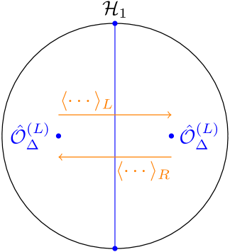
(a)

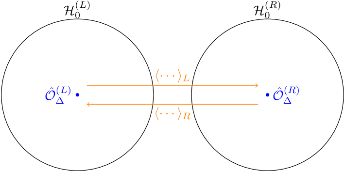
(b)

Figure 8: Conversion property (236a) for operators $\hat{\mathcal{O}}^{L/R}_{\Delta}$in the double-scaled algebra acting on (a) $\mathcal{H}_{1}$, or (b) $\mathcal{H}_{0}^{L}\otimes\mathcal{H}_{0}^{R}$, which are related thought the isometric map $\hat{\mathcal{F}}$ (194).

Appendix G Properties of the OTOC

In this appendix we discuss different properties of the semiclassical OTOC (33) that we derived in Sec. 2.3 in relation with related literature.

A bound on OTOC

It is interesting to compare our explicit results with bounds on the growth of OTOCs in the literature. In particular, Milekhin:2024vbb found that, considering fermionic systems at infinite temperature, the following OTOCs can be bounded in terms of two-point functions at infinite temperature

$$\absolutevalue{\expectationvalue{\hat{\mathcal{O}}_{\Delta}(t)\hat{\mathcal{O}}_{\Delta}(0)\hat{\mathcal{O}}_{\Delta}(t)\hat{\mathcal{O}}_{\Delta}(0)}}\geq 2{G}^{(\Delta)}(t)^{2}-1\leavevmode\nobreak\ ,$$ (237)

$$\absolutevalue{\expectationvalue{\hat{\mathcal{O}}_{\Delta}(t)\hat{\mathcal{O}}_{\Delta}(0)\hat{\mathcal{O}}_{\Delta}(t)\hat{\mathcal{O}}_{\Delta}(0)}}\geq G^{(\Delta)}(t)^{2}\leavevmode\nobreak\ .$$ (238)

where $G^{(\Delta)}(t)$ is a two-point correlation function. The first and second inequalities above were denoted as weak and strong bounds on OTOC growth by Milekhin:2024vbb .

One can explicitly check the strong version of the bound by inserting both the crossed four-point function (32) at leading order in the $\lambda\rightarrow 0$ limit, and the thermal two-point function $G^{(\Delta)}(t)$ (150) in $\mathcal{H}_{0}$ into (238):

$$\quantity(\frac{1}{\cosh^{2}(Jt)-q^{\Delta_{\rm S}}\sinh^{2}(Jt)})^{2\Delta_{w}}\geq\quantity(\frac{1}{\cosh^{2}(Jt)})^{2\Delta_{w}}\leavevmode\nobreak\ .$$ (239)

The bound above is always explicitly satisfied since $q^{\Delta_{\rm S}}>0$. Similarly for (238),

$$\quantity(\frac{1}{\cosh^{2}(Jt)-q^{\Delta_{\rm S}}\sinh^{2}(Jt)})^{2\Delta_{w}}\geq 2\quantity(\frac{1}{\cosh^{2}(Jt)})^{2\Delta_{w}}-1\leavevmode\nobreak\ .,$$ (240)

since both sides in (240) are monotonically decreasing, and the bound is saturated at $t=0$. Thus, we see that the bound (238) is explicitly obeyed at all times in this system. Meanwhile, Milekhin:2024vbb found that (238) holds at early times in generic fermionic systems (based on numerical evidence).

(Sub-)maximal chaos

On the other hand, we are interested in finite temperature effects in the evolution of the OTOC (32). Considering the same time regimes as (71, 73) for the OTOC (32), we recover

$$\evaluated{G_{\tilde{\Delta}}^{(\Delta_{w})}(-\tau,\tau)}_{\tau=\frac{\beta(\theta)}{2}+\mathrm{i}t}$$ (241)

$$=\langle\mathrm{e}^{\frac{\beta}{2}(\theta)\hat{H}_{L}}\hat{\mathcal{O}}_{\Delta_{\rm S}}(t_{L})\mathrm{e}^{-\frac{\beta(\theta)}{2}\hat{H}_{L}}\leavevmode\hbox to18.3pt{\vbox to9.72pt{\text{[drawing]}}}(0)\mathrm{e}^{-\frac{\beta(\theta)}{2}\hat{H}_{L}}\hat{\mathcal{O}}_{\Delta_{\rm S}}(t_{L})\mathrm{e}^{\frac{\beta(\theta)}{2}\hat{H}_{L}}\leavevmode\hbox to18.3pt{\vbox to9.72pt{\text{[drawing]}}}\leavevmode\hbox to0pt{\vbox to0pt{\text{[drawing]}}}(0)\rangle\vbox to15.99992pt{}{} \hat{\mathcal{O}}_{\Delta_{w}} \hat{\mathcal{O}}_{\Delta_{w}}$$

$$= \quantity(A(\theta,-q^{\Delta})+B(\theta,-q^{\Delta})\cosh(2J\sin\theta t))^{-2\Delta_{w}}$$

$$=$$

where ${\beta}_{\rm fake}=\frac{4\pi}{J\sin\theta}$, and $A(\theta,q^{\Delta})$, $B(\theta,q^{\Delta})$ and $t_{\rm sc}$ are in (64), (65) and (72) respectively. Let us compare with the chaos bound conjecture in Maldacena:2015waa , which states that the maximal Lyapunov exponent of an OTOC in generic quantum systems is given by the factor $\frac{\beta}{2\pi}$. In contrast, (241) is submaximally chaotic in the OTOC sense Maldacena:2015waa when we compare the exponent at $t\in[(J\sin\theta)^{-1},\leavevmode\nobreak\ t_{\rm sc}]$ with respect to the physical temperature (in the microcanonical ensemble (148)) $\beta(\theta)=(1-\frac{2\theta}{\pi})\beta_{\rm fake}$. Similar observations for two-point functions in $\mathcal{H}_{0}$ appeared in Blommaert:2024ydx .

Hyperfast growth

We remark that (72) displays a hyperfast growth, in the sense of Anegawa:2024yia (and it also agrees with their estimate). Namely, the scrambling time of the DSSYK model with matter chords is independent of the size of the system, which would correspond to the total number of fermions in the original DSSYK Hamiltonian (130) (which is implicit in $q$). This can be contrasted with the fast-scrambling conjecture in Sekino:2008he . It was argued that the fastest scrambling time for information recovery scales is of the order $\log(S)$, where $S$ is the entropy of the system. One might argue that the definitions of scrambling time we are comparing are different and thus it is not surprising they can scale differently. However, as we have shown, the scrambling time in Krylov operator complexity (70) is determined by an OTOC in (59). This implies that the scrambling time in Krylov complexity, in this particular system, coincides with the scrambling time of an OTOC (defined as the time for the exponential growth to become small). We may then associate the scrambling time with the transition to late linear growth of the OTOC. Thus, the DSSYK model with matter behaves as a hyperfast scrambler of information in a closely related notion to the one proposed in Sekino:2008he .

Appendix H Krylov basis and Lanczos coefficients in the one-particle chord space

In this appendix, we fill in some of the technical details in the Lanczos algorithm (51). We find the Krylov basis and the Lanczos coefficients in the semiclassical limit, taking similar steps as Ambrosini:2024sre .

Lanczos coefficients and the Krylov basis

We begin proposing an Ansatz for the Krylov basis. Based on the work by Ambrosini:2024sre , we search for a decomposition of the Krylov basis as $\ket{K_{n}^{(\eta)}}=\ket{k_{n}^{(\eta)}}+$additional state, where $\ket{k_{n}^{(\eta)}}$ appears in (49), and it indeed solves the algorithm (50) exactly up to $n=3$. The additional state is determined by tridiagonalizing the Liouvillian $\mathcal{L}_{\eta}\propto(\hat{a}_{R}+\eta\hat{a}_{L}+\hat{a}^{\dagger}_{R}+\eta\hat{a}^{\dagger}_{L})$ (155). For this reason, we evaluate

$$\mathcal{L}_{\eta}\ket{k_{n}^{(\eta)}}= \frac{J\leavevmode\nobreak\ c^{(\eta)}_{n}}{\sqrt{\lambda}}(\hat{a}_{R}+\eta\hat{a}_{L}+\hat{a}^{\dagger}_{R}+\eta\hat{a}^{\dagger}_{L})\sum_{k=0}^{n}\eta^{k}\begin{pmatrix}n\\ k\end{pmatrix}\ket{\Delta_{\rm S};k,n-k}\leavevmode\nobreak\ ,$$ (242)

where

$$(\hat{a}^{\dagger}_{R}+\eta\hat{a}^{\dagger}_{L})\sum_{k=0}^{n}\eta^{k}\begin{pmatrix}n\\ k\end{pmatrix}\ket{\Delta_{\rm S};k,n-k}=\sum_{k=0}^{n+1}\eta^{k}\begin{pmatrix}n+1\\ k\end{pmatrix}\ket{\Delta_{\rm S};k,n+1-k}\leavevmode\nobreak\ ,$$ (243)

$$(\hat{a}_{R}+\eta\hat{a}_{L})\sum_{k=0}^{n}\eta^{k}\begin{pmatrix}n\\ k\end{pmatrix}\ket{\Delta_{\rm S};k,n-k}=\sum_{k=0}^{n-1}Z^{(\eta)}_{k}(n)\eta^{k}\begin{pmatrix}n-1\\ k\end{pmatrix}\ket{\Delta_{\rm S};k,n-1-k}$$ (244)

$$\text{with}\quad Z^{(\eta)}_{k}(n)=\frac{n[n-k]_{q}}{n-k}(1+\eta q^{\Delta_{\rm S}+k})+\frac{n[k+1]_{q}}{k+1}(1+\eta q^{\Delta_{\rm S}+n-1-k})\leavevmode\nobreak\ .$$

In the first equality, we used $\begin{pmatrix}n\\ k\end{pmatrix}+\begin{pmatrix}n\\ k-1\end{pmatrix}=\begin{pmatrix}n+1\\ k\end{pmatrix}$, and in the second one (156, 157):

$$\hat{a}_{R}+\eta\hat{a}_{L}=\hat{\alpha}_{L}[n_{L}]_{q}(1+\eta q^{\Delta_{\rm S}+n_{R}})+\hat{\alpha}_{R}[n_{R}]_{q}(1+\eta q^{\Delta_{\rm S}+n_{L}})\leavevmode\nobreak\ .$$ (245)

Collecting the relations, we can then write:

$$\mathcal{L}_{\eta}\ket{k_{n}^{(\eta)}}= b_{n+1}\ket{k_{n+1}^{(\eta)}}+b_{n}\ket{k_{n-1}^{(\eta)}}$$ (246)

$$+\sum_{k=0}^{n-1}\quantity(Z^{(\eta)}_{k}(n)-Z^{(\eta)}_{n/2}(n))\begin{pmatrix}n-1\\ k\end{pmatrix}\eta^{k}\ket{\Delta_{\rm S};k,n-1-k}\leavevmode\nobreak\ ,$$

where $\ket{k_{n-1}^{(\eta)}}=c_{n}^{(\eta)}\sum_{k=0}^{n}\eta^{k}\begin{pmatrix}n\\ k\end{pmatrix}\ket{\Delta_{\rm S};k,n-k}$, and

$$b^{(\eta)}_{n}\underset{\lambda\rightarrow 0}{=}J\sqrt{Z^{(\eta)}_{n/2}(n)}\leavevmode\nobreak\ ,\quad c_{n}^{(\eta)}={J^{n}}\prod_{i=1}^{n}(b_{n}^{(\eta)})^{-1}\leavevmode\nobreak\ .$$ (247)

In the semiclassical limit (i.e. $\lambda n$ fixed as $\lambda\rightarrow 0$ Lin:2022rbf ; Lin:2023trc ; Rabinovici:2023yex ), the binomial factor $\begin{pmatrix}n\\ k\end{pmatrix}$ localizes at $k=n/2$ when $\eta=\pm 1$; while for $\eta\in\mathbb{R}$ $k=\eta n/(1+\eta)$ Ambrosini:2024sre . This means that the last term in (246) is negligible compared to $\quantity{\ket{k_{n}^{(\eta)}}}$ in the semiclassical limit when $\eta=\pm 1$. For more general $\eta$ the term does not cancel out, and thus we would not solve the two-sided Lanczos algorithm. In principle, there might be a different ansatz instead of (49) that one should use to work on the more general case.

Thus, from (247) we find the Lanczos coefficients in the algorithm (50)

$$a^{(\eta)}_{n}=0\leavevmode\nobreak\ ,\quad b^{(\eta)}_{n}\underset{\lambda\rightarrow 0}{=}\frac{2J}{\sqrt{\lambda(1-q)}}\sqrt{(1-q^{n/2})(1+\eta q^{n/2+\Delta_{\rm S}})}\leavevmode\nobreak\ ,$$ (248)

and the normalization constants of $\ket{k_{n}^{(\eta)}}$,

$$\lim_{\lambda\rightarrow 0}c^{(\eta)}_{n}=\lim_{\lambda\rightarrow 0}\sqrt{\frac{\lambda^{n}(1-q)^{n}(1+\eta)}{2^{n}(q^{1/2};q^{1/2})_{n}(-\eta;q^{1/2})_{n+1}}}=\sqrt{\frac{\lambda^{n}}{n!(1+\eta)^{n}}}\leavevmode\nobreak\ ,\quad\text{for }\eta\neq 1\leavevmode\nobreak\ .$$ (249)

The case $\eta=-1$ is studied in AX .

Generalized wavefunctions

We would like to find explicit expressions for the wavefunctions of the form

$${\Psi}^{(\eta)}_{n}(\tau)=\bra{k^{(\eta)}_{n}}\mathrm{e}^{-\mathcal{L}_{\eta}}\ket{\Psi_{\tilde{\Delta}}(\tau_{L}=\eta\tau,\tau_{R}=\tau)}\leavevmode\nobreak\ ,$$ (250)

which are the coefficients of the total chord number basis $\quantity{\ket{k_{n}^{(\eta)}}}$ (55). In the $\lambda\rightarrow 0$ limit, the Krylov space of the two-sided HH state (7) becomes:

$$\Psi_{n}^{(\eta)}(\tau)= c_{n}^{(\eta)}\bra{\Psi_{\tilde{\Delta}}(\eta\tau,\tau)}\sum_{k}\eta^{k}\begin{pmatrix}n\\ k\end{pmatrix}\ket{\Delta_{\rm S};k,n-k}$$ (251)

$$= c_{n}^{(\eta)}\sum_{k}\eta^{k}\begin{pmatrix}n\\ k\end{pmatrix}\bra{\Delta_{\rm S};0,0}\mathrm{e}^{-\tau(\hat{H}_{R}+\eta\hat{H}_{L})}\ket{\Delta_{\rm S};k,n-k}$$ (252)

$$= c_{n}^{(\eta)}\int\mathrm{d}\mu(\theta_{L})\mathrm{d}\mu(\theta_{R})\frac{(q^{\Delta_{\rm S}};q)_{\infty}}{(q^{\Delta_{\rm S}}\mathrm{e}^{\pm\mathrm{i}\theta_{L}\pm\mathrm{i}\theta_{R}};q)_{\infty}}\mathrm{e}^{-\tau(\eta E(\theta_{L})+E(\theta_{R}))}\cdot$$ (253)

$$\qquad\cdot\sum_{k}\eta^{k}\begin{pmatrix}n\\ k\end{pmatrix}\frac{H_{k}(\cos\theta_{L}|q)H_{n-k}(\cos\theta_{R}|q)}{\sqrt{(q;q)_{k}(q;q)_{n-k}}}\leavevmode\nobreak\ ,$$

where $c_{n}^{(\eta)}$ is a normalization constant (55), and we used (139) to express

$$(\theta_{L},\theta_{R}|k,n-k)=\frac{H_{k}(\cos\theta_{L}|q)H_{n-k}(\cos\theta_{R}|q)}{\sqrt{(q;q)_{k}(q;q)_{n-k}}}\leavevmode\nobreak\ .$$ (254)

As a future direction, this form of the amplitudes could be evaluated numerically in the $\lambda\rightarrow 0$ limit to test our results from classical phase space methods (29a). Namely, to determine Krylov complexity for $\eta=\pm 1$,

$$\mathcal{C}^{(\eta)}(t)=\frac{\sum_{n}n\absolutevalue{\Psi_{n}^{(\eta)}(\frac{\beta(\theta)}{2})+\mathrm{i}t)}^{2}}{\sum_{n}\absolutevalue{\Psi_{n}^{\eta}(\frac{\beta(\theta)}{2})}^{2}}\leavevmode\nobreak\ .$$ (255)

Appendix I Non-composite many particle chord states

In this appendix we construct PETS for non-composite many particle chord operators acting on the tracial state $\ket{0}$, states on $\mathcal{H}_{m\in\mathbb{Z}_{\geq 0}}$. This allows to generalize our discussion on composite operators acting on the tracial state to evaluate dynamical observables in thermal ensembles, such as (7). We are particularly interested in states of the form

$$\mathrm{e}^{-\tau_{0}\hat{H}_{L}}\hat{\mathcal{O}}_{\Delta_{1}}\mathrm{e}^{-\tau_{1}\hat{H}_{L}}\hat{\mathcal{O}}_{\Delta_{2}}\cdots\mathrm{e}^{-\tau_{m-1}\hat{H}_{L}}\hat{\mathcal{O}}_{\Delta_{m}}\mathrm{e}^{-\tau_{m}\hat{H}_{L}}\ket{0}\leavevmode\nobreak\ ,$$ (256)

to derive an explicit decomposition in the $\mathcal{H}_{0}$ and $\mathcal{H}_{1}$ irreps.

We start from $\hat{\mathcal{O}}_{\Delta}=b^{\dagger}_{\Delta}+b_{\Delta}$ with $b^{\dagger}_{\Delta}$, $b_{\Delta}$ in (158, 159). The simplest non-trivial example of (256) is $m=1$, where

$$\ket{\Psi_{\Delta_{1}}(\tau_{0},\tau_{1})}=\mathrm{e}^{-\tau_{0}\hat{H}_{L}}\hat{\mathcal{O}}^{L}_{\Delta_{1}}\mathrm{e}^{-\tau_{1}\hat{H}_{L}}\ket{0}=\sum_{n_{0},n_{1}}\phi_{n_{0}}(\tau_{0})\phi_{n_{1}}(\tau_{1})\ket{\Delta;n_{0},n_{1}}\leavevmode\nobreak\ ,$$ (257)

where $\phi_{n}(\tau)=\bra{n}\mathrm{e}^{-\tau\hat{H}}\ket{0}$, and in the last step we used the isometric map $\hat{\mathcal{F}}$ (194) (similar to (5.6) in Xu:2024gfm ).

Moving on to $m=2$ case in (256),

$$\ket{\Psi_{\Delta_{1},\Delta_{2}}(\tau_{0},\tau_{1},\tau_{2})}=\mathrm{e}^{-\tau_{0}\hat{H}_{L}}\hat{\mathcal{O}}_{\Delta}\mathrm{e}^{-\tau_{1}\hat{H}_{L}}\hat{\mathcal{O}}_{\Delta}\mathrm{e}^{-\tau_{2}\hat{H}_{L}}\ket{0}\leavevmode\nobreak\ .$$ (258)

We need to distinguish between two cases. For $\Delta_{1}=\Delta_{2}=\Delta$:

$$\ket{\Psi_{\Delta,\Delta}(\tau_{0},\tau_{1},\tau_{2})}$$ (259)

$$=\sum_{n_{1},n_{2}}\phi_{n_{1}}(\tau_{1})\phi_{n_{2}}(\tau_{2})\quantity(q^{n_{1}}\mathrm{e}^{-\tau_{0}\hat{H}}\ket{n_{1}+n_{2}}+\sum_{n_{0}}\phi_{n_{0}}(\tau_{0})\ket{\Delta^{(2)};n_{0},n_{1},n_{2}})\leavevmode\nobreak\ ,$$

$$=\sum_{n_{0},n_{1},n_{2}=0}^{\infty}\biggl{(}q^{n_{1}}\phi^{(n_{1}+n_{2})}_{n_{0}}(\tau_{0})\ket{n_{0}}$$

$$\qquad+\phi_{n_{1}}(\tau_{1})\phi_{n_{2}}(\tau_{2})\sum_{l+m_{L}+m_{R}=n_{1}}\chi_{l,m_{L},m_{R}}\ket{2\Delta+l;n_{0}+m_{L},n_{2}+m_{R}}\biggr{)}\leavevmode\nobreak\ ,$$

where $\phi^{(n_{1}+n_{2})}_{n_{0}}(\tau_{0})\equiv\bra{n_{0}}\mathrm{e}^{-\tau_{0}\hat{H}}\ket{n_{1}+n_{2}}$, $\Delta^{(2)}=\quantity{\Delta,\Delta}$, and we have applied (10) in the last line.

Meanwhile, $\Delta_{1}\neq\Delta_{2}$:

$$\ket{\Psi_{\Delta_{1},\Delta_{2}}(\tau_{0},\tau_{1},\tau_{2})}=\sum_{n_{0},n_{1},n_{2}}\phi_{n_{0}}(\tau_{0})\phi_{n_{1}}(\tau_{1})\phi_{n_{2}}(\tau_{2})\ket{\Delta_{1},\Delta_{2};n_{0},n_{1},n_{2}}$$ (260)

$${=\sum_{n_{0},n_{1},n_{2}=0}^{\infty}\phi_{n_{0}}(\tau_{0})\phi_{n_{1}}(\tau_{1})\phi_{n_{2}}(\tau_{2})\sum_{l+m_{L}+m_{R}=n_{1}}\chi_{l,m_{L},m_{R}}\ket{\Delta_{1}+\Delta_{2}+l;m_{L}+n_{0},m_{R}+n_{2}}\leavevmode\nobreak\ .}$$

Now that we have recovered a explicit form of the non-composite two particle PETS. One may continue recursively to express the most general double-scaled PETS (6) into the zero and one-particle irreps. The price to pay is the addition of the Clebsch–Gordan coefficients. A key advantage of our procedure is that, the integration measure in energy basis is known for the zero and one-particle irreps. One can therefore use (259 or 260) to explicitly evaluate partition functions and two (or higher)-point correlation functions (analogous to App. D and E respectively), which we leave for future directions.

References

- (1) H.W. Lin, The bulk Hilbert space of double scaled SYK, JHEP 11 (2022) 060 [2208.07032].
- (2) M. Berkooz, P. Narayan and J. Simon, Chord diagrams, exact correlators in spin glasses and black hole bulk reconstruction, JHEP 08 (2018) 192 [1806.04380].
- (3) M. Berkooz, M. Isachenkov, V. Narovlansky and G. Torrents, Towards a full solution of the large N double-scaled SYK model, JHEP 03 (2019) 079 [1811.02584].
- (4) M. Berkooz and O. Mamroud, A cordial introduction to double scaled SYK, Rept. Prog. Phys. 88 (2025) 036001 [2407.09396].
- (5) M. Berkooz, R. Frumkin, O. Mamroud and J. Seitz, Twisted times, the Schwarzian and its deformations in DSSYK, 2412.14238.
- (6) R. Jackiw, Lower dimensional gravity, Nuclear Physics B 252 (1985) 343.
- (7) C. Teitelboim, Gravitation and hamiltonian structure in two spacetime dimensions, Physics Letters B 126 (1983) 41.
- (8) K. Okuyama, De Sitter JT gravity from double-scaled SYK, 2505.08116.
- (9) L. Susskind, Entanglement and Chaos in De Sitter Space Holography: An SYK Example, JHAP 1 (2021) 1 [2109.14104].
- (10) L. Susskind, De Sitter Space, Double-Scaled SYK, and the Separation of Scales in the Semiclassical Limit, 2209.09999.
- (11) H. Lin and L. Susskind, Infinite Temperature’s Not So Hot, 2206.01083.
- (12) A.A. Rahman, dS JT Gravity and Double-Scaled SYK, 2209.09997.
- (13) A.A. Rahman and L. Susskind, Comments on a Paper by Narovlansky and Verlinde, 2312.04097.
- (14) A.A. Rahman and L. Susskind, -Chords, Wee-Chords, and de Sitter Space, 2407.12988.
- (15) A.A. Rahman and L. Susskind, Infinite Temperature is Not So Infinite: The Many Temperatures of de Sitter Space, 2401.08555.
- (16) V. Narovlansky and H. Verlinde, Double-scaled SYK and de Sitter holography, JHEP 05 (2025) 032 [2310.16994].
- (17) H. Verlinde, Double-scaled SYK, chords and de Sitter gravity, JHEP 03 (2025) 076 [2402.00635].
- (18) H. Verlinde, Talks given at the QGQC5 conference, UC Davis; the Franqui Symposium, Brussels; ‘Quantum Gravity on Southern Cone’, Argentina; and ‘SYK models and Gauge Theory’ workshop at Weizmann Institute, 2019.
- (19) H. Verlinde and M. Zhang, SYK Correlators from 2D Liouville-de Sitter Gravity, 2402.02584.
- (20) D. Gaiotto and H. Verlinde, SYK-Schur duality: Double scaled SYK correlators from supersymmetric gauge theory, 2409.11551.
- (21) D. Tietto and H. Verlinde, A microscopic model of de Sitter spacetime with an observer, 2502.03869.
- (22) A. Milekhin and J. Xu, Revisiting Brownian SYK and its possible relations to de Sitter, 2312.03623.
- (23) H. Yuan, X.-H. Ge and K.-Y. Kim, Pole-skipping in two-dimensional de Sitter spacetime and double-scaled SYK model, 2408.12330.
- (24) S.E. Aguilar-Gutierrez, Towards complexity in de Sitter space from the double-scaled Sachdev-Ye-Kitaev model, JHEP 10 (2024) 107 [2403.13186].
- (25) A. Blommaert, T.G. Mertens and S. Yao, Dynamical actions and q-representation theory for double-scaled SYK, JHEP 02 (2024) 067 [2306.00941].
- (26) A. Blommaert, A. Levine, T.G. Mertens, J. Papalini and K. Parmentier, An entropic puzzle in periodic dilaton gravity and DSSYK, 2411.16922.
- (27) A. Blommaert, T.G. Mertens and J. Papalini, The dilaton gravity hologram of double-scaled SYK, 2404.03535.
- (28) A. Blommaert, A. Levine, T.G. Mertens, J. Papalini and K. Parmentier, Wormholes, branes and finite matrices in sine dilaton gravity, 2501.17091.
- (29) S.E. Aguilar-Gutierrez, forthcoming, 2025.
- (30) J. Xu, Von Neumann Algebras in Double-Scaled SYK, 2403.09021.
- (31) M. Berkooz, N. Brukner, S.F. Ross and M. Watanabe, Going beyond ER=EPR in the SYK model, JHEP 08 (2022) 051 [2202.11381].
- (32) V. Balasubramanian, P. Caputa, J.M. Magan and Q. Wu, Quantum chaos and the complexity of spread of states, Phys. Rev. D 106 (2022) 046007 [2202.06957].
- (33) D.E. Parker, X. Cao, A. Avdoshkin, T. Scaffidi and E. Altman, A Universal Operator Growth Hypothesis, Phys. Rev. X 9 (2019) 041017 [1812.08657].
- (34) E. Rabinovici, A. Sánchez-Garrido, R. Shir and J. Sonner, A bulk manifestation of Krylov complexity, JHEP 08 (2023) 213 [2305.04355].
- (35) L. Bossi, L. Griguolo, J. Papalini, L. Russo and D. Seminara, Sine-dilaton gravity vs double-scaled SYK: exploring one-loop quantum corrections, 2411.15957.
- (36) M.P. Heller, J. Papalini and T. Schuhmann, Krylov spread complexity as holographic complexity beyond JT gravity, 2412.17785.
- (37) H.W. Lin and D. Stanford, A symmetry algebra in double-scaled SYK, SciPost Phys. 15 (2023) 234 [2307.15725].
- (38) J. Xu, On Chord Dynamics and Complexity Growth in Double-Scaled SYK, 2411.04251.
- (39) M. Ambrosini, E. Rabinovici, A. Sánchez-Garrido, R. Shir and J. Sonner, Operator K-complexity in DSSYK: Krylov complexity equals bulk length, 2412.15318.
- (40) L. Susskind, Computational Complexity and Black Hole Horizons, Fortsch. Phys. 64 (2016) 24 [1403.5695].
- (41) D. Stanford and L. Susskind, Complexity and Shock Wave Geometries, Phys. Rev. D 90 (2014) 126007 [1406.2678].
- (42) S.E. Aguilar-Gutierrez and J. Xu, forthcoming, 2025.
- (43) B. Bhattacharjee, P. Nandy and T. Pathak, Krylov complexity in large q and double-scaled SYK model, JHEP 08 (2023) 099 [2210.02474].
- (44) T. Anegawa and R. Watanabe, Krylov complexity of fermion chain in double-scaled SYK and power spectrum perspective, 2407.13293.
- (45) P. Nandy, Tridiagonal Hamiltonians modeling the density of states of the Double-Scaled SYK model, 2410.07847.
- (46) V. Balasubramanian, J.M. Magan, P. Nandi and Q. Wu, Spread complexity and the saturation of wormhole size, 2412.02038.
- (47) M. Miyaji, S. Mori and K. Okuyama, Finite Bulk Hilbert Space in ETH Matrix Model for double-scaled SYK, 2505.13194.
- (48) A. Goel, H.T. Lam, G.J. Turiaci and H. Verlinde, Expanding the Black Hole Interior: Partially Entangled Thermal States in SYK, JHEP 02 (2019) 156 [1807.03916].
- (49) A. Goel, V. Narovlansky and H. Verlinde, Semiclassical geometry in double-scaled SYK, JHEP 11 (2023) 093 [2301.05732].
- (50) A. Milekhin and J. Xu, On scrambling, tomperature and superdiffusion in de Sitter space, 2403.13915.
- (51) P. Caputa, B. Chen, R.W. McDonald, J. Simón and B. Strittmatter, Spread Complexity Rate as Proper Momentum, 2410.23334.
- (52) P. Caputa and G. Di Giulio, Local Quenches from a Krylov Perspective, 2502.19485.
- (53) Z.-Y. Fan, Momentum-Krylov complexity correspondence, 2411.04492.
- (54) P.-Z. He, Revisit the relationship between spread complexity rate and radial momentum, 2411.19172.
- (55) L. Susskind, Why do Things Fall?, 1802.01198.
- (56) L. Susskind, Complexity and Newton’s Laws, Front. in Phys. 8 (2020) 262 [1904.12819].
- (57) L. Susskind and Y. Zhao, Complexity and Momentum, JHEP 03 (2021) 239 [2006.03019].
- (58) S.-K. Jian, B. Swingle and Z.-Y. Xian, Complexity growth of operators in the SYK model and in JT gravity, JHEP 03 (2021) 014 [2008.12274].
- (59) J.L.F. Barbón, J. Martín-García and M. Sasieta, Momentum/Complexity Duality and the Black Hole Interior, JHEP 07 (2020) 169 [1912.05996].
- (60) J.L.F. Barbon, J. Martin-Garcia and M. Sasieta, Proof of a Momentum/Complexity Correspondence, Phys. Rev. D 102 (2020) 101901 [2006.06607].
- (61) J.L.F. Barbon, J. Martin-Garcia and M. Sasieta, A Generalized Momentum/Complexity Correspondence, JHEP 04 (2021) 250 [2012.02603].
- (62) S.H. Shenker and D. Stanford, Black holes and the butterfly effect, JHEP 03 (2014) 067 [1306.0622].
- (63) S. Xu and B. Swingle, Scrambling Dynamics and Out-of-Time-Ordered Correlators in Quantum Many-Body Systems, PRX Quantum 5 (2024) 010201 [2202.07060].
- (64) Y. Sekino and L. Susskind, Fast Scramblers, JHEP 10 (2008) 065 [0808.2096].
- (65) J. Maldacena, S.H. Shenker and D. Stanford, A bound on chaos, JHEP 08 (2016) 106 [1503.01409].
- (66) A. Belaey, T.G. Mertens and T. Tappeiner, Quantum group origins of edge states in double-scaled SYK, 2503.20691.
- (67) T.G. Mertens, G.J. Turiaci and H.L. Verlinde, Solving the Schwarzian via the Conformal Bootstrap, JHEP 08 (2017) 136 [1705.08408].
- (68) H.T. Lam, T.G. Mertens, G.J. Turiaci and H. Verlinde, Shockwave S-matrix from Schwarzian Quantum Mechanics, JHEP 11 (2018) 182 [1804.09834].
- (69) T.G. Mertens and G.J. Turiaci, Solvable models of quantum black holes: a review on Jackiw–Teitelboim gravity, Living Rev. Rel. 26 (2023) 4 [2210.10846].
- (70) M. Duetsch and K.-H. Rehren, Generalized free fields and the AdS - CFT correspondence, Annales Henri Poincare 4 (2003) 613 [math-ph/0209035].
- (71) G.W. Gibbons, S.W. Hawking and M.J. Perry, Path Integrals and the Indefiniteness of the Gravitational Action, Nucl. Phys. B 138 (1978) 141.
- (72) R. Monteiro, M.J. Perry and J.E. Santos, Thermodynamic instability of rotating black holes, Phys. Rev. D 80 (2009) 024041 [0903.3256].
- (73) R. Monteiro and J.E. Santos, Negative modes and the thermodynamics of Reissner-Nordstrom black holes, Phys. Rev. D 79 (2009) 064006 [0812.1767].
- (74) T. Prestidge, Dynamic and thermodynamic stability and negative modes in Schwarzschild-anti-de Sitter, Phys. Rev. D 61 (2000) 084002 [hep-th/9907163].
- (75) D. Marolf and J.E. Santos, AdS Euclidean wormholes, Class. Quant. Grav. 38 (2021) 224002 [2101.08875].
- (76) D. Marolf, Gravitational thermodynamics without the conformal factor problem: partition functions and Euclidean saddles from Lorentzian path integrals, JHEP 07 (2022) 108 [2203.07421].
- (77) J. Erdmenger, S.-K. Jian and Z.-Y. Xian, Universal chaotic dynamics from Krylov space, JHEP 08 (2023) 176 [2303.12151].
- (78) N. Afkhami-Jeddi, T. Hartman, S. Kundu and A. Tajdini, Shockwaves from the Operator Product Expansion, JHEP 03 (2019) 201 [1709.03597].
- (79) Y. Jia, Contact diagrams for chords, 2503.22619.
- (80) M. Berkooz, N. Brukner, Y. Jia and O. Mamroud, From Chaos to Integrability in Double Scaled SYK, 2403.01950.
- (81) M. Berkooz, N. Brukner, Y. Jia and O. Mamroud, A Path Integral for Chord Diagrams and Chaotic-Integrable Transitions in Double Scaled SYK, 2403.05980.
- (82) J.S. Cotler, G. Gur-Ari, M. Hanada, J. Polchinski, P. Saad, S.H. Shenker et al., Black Holes and Random Matrices, JHEP 05 (2017) 118 [1611.04650].
- (83) S. Chapman and G. Policastro, Quantum computational complexity from quantum information to black holes and back, Eur. Phys. J. C 82 (2022) 128 [2110.14672].
- (84) P. Nandy, A.S. Matsoukas-Roubeas, P. Martínez-Azcona, A. Dymarsky and A. del Campo, Quantum Dynamics in Krylov Space: Methods and Applications, 2405.09628.
- (85) A. Sánchez-Garrido, On Krylov Complexity, other thesis, University of Geneva, 7, 2024, [2407.03866].
- (86) H.A. Camargo, Y. Fu, V. Jahnke, K. Pal and K.-Y. Kim, Quantum Signatures of Chaos from Free Probability, 2503.20338.
- (87) E. Gesteau, Emergent spacetime and the ergodic hierarchy, Phys. Rev. D 110 (2024) 106005 [2310.13733].
- (88) K. Furuya, N. Lashkari, M. Moosa and S. Ouseph, Information loss, mixing and emergent type III1 factors, JHEP 08 (2023) 111 [2305.16028].
- (89) A. Belin, R.C. Myers, S.-M. Ruan, G. Sárosi and A.J. Speranza, Does Complexity Equal Anything?, Phys. Rev. Lett. 128 (2022) 081602 [2111.02429].
- (90) A. Blommaert, T.G. Mertens and S. Yao, The q-Schwarzian and Liouville gravity, 2312.00871.
- (91) S.H. Shenker and D. Stanford, Multiple Shocks, JHEP 12 (2014) 046 [1312.3296].
- (92) K. Goto, H. Marrochio, R.C. Myers, L. Queimada and B. Yoshida, Holographic Complexity Equals Which Action?, JHEP 02 (2019) 160 [1901.00014].
- (93) S.E. Aguilar-Gutierrez, C=Anything and the switchback effect in Schwarzschild-de Sitter space, JHEP 03 (2024) 062 [2309.05848].
- (94) D. Harlow and D. Jafferis, The Factorization Problem in Jackiw-Teitelboim Gravity, JHEP 02 (2020) 177 [1804.01081].
- (95) L.D. Faddeev, The feynman integral for singular lagrangians, Teoreticheskaya i Matematicheskaya Fizika 1 (1969) 3.
- (96) P.A.M. Dirac, Quantised singularities in the electromagnetic field,, Proc. Roy. Soc. Lond. A 133 (1931) 60.
- (97) P.A. Dirac, Lectures on quantum mechanics, Courier Corporation (2013).
- (98) G. Kunstatter, Geometrical approach to the effective action, in Banff Summer Institute: Gravitation, 10, 1990.
- (99) L. Susskind, Black Holes Hint towards De Sitter Matrix Theory, Universe 9 (2023) 368 [2109.01322].
- (100) V. Chandrasekaran, R. Longo, G. Penington and E. Witten, An algebra of observables for de Sitter space, JHEP 02 (2023) 082 [2206.10780].
- (101) V. Chandrasekaran, G. Penington and E. Witten, Large N algebras and generalized entropy, JHEP 04 (2023) 009 [2209.10454].
- (102) G. Penington and E. Witten, Algebras and States in JT Gravity, 2301.07257.
- (103) E. Witten, Algebras, Regions, and Observers, 2303.02837.
- (104) E. Witten, A Background Independent Algebra in Quantum Gravity, Gen. Rel. Grav. 57 (2025) 17.
- (105) G. Penington and E. Witten, Algebras and states in super-JT gravity, 2412.15549.
- (106) E. Witten, A background-independent algebra in quantum gravity, JHEP 03 (2024) 077 [2308.03663].
- (107) E. Witten, Gravity and the crossed product, JHEP 10 (2022) 008 [2112.12828].
- (108) J. De Vuyst, S. Eccles, P.A. Hoehn and J. Kirklin, Gravitational entropy is observer-dependent, 2405.00114.
- (109) J. De Vuyst, S. Eccles, P.A. Hoehn and J. Kirklin, Crossed products and quantum reference frames: on the observer-dependence of gravitational entropy, 2412.15502.
- (110) K. Jensen, J. Sorce and A.J. Speranza, Generalized entropy for general subregions in quantum gravity, JHEP 12 (2023) 020 [2306.01837].
- (111) T. Faulkner and A.J. Speranza, Gravitational algebras and the generalized second law, JHEP 11 (2024) 099 [2405.00847].
- (112) J. Kudler-Flam, S. Leutheusser and G. Satishchandran, Algebraic Observational Cosmology, 2406.01669.
- (113) S. Ali Ahmad and R. Jefferson, Crossed product algebras and generalized entropy for subregions, SciPost Phys. Core 7 (2024) 020 [2306.07323].
- (114) J. Kudler-Flam, S. Leutheusser and G. Satishchandran, Generalized black hole entropy is von Neumann entropy, Phys. Rev. D 111 (2025) 025013 [2309.15897].
- (115) H. Tang, Entanglement entropy in type II1 von Neumann algebra: examples in Double-Scaled SYK, 2404.02449.
- (116) H. Tang, Operator Krylov complexity in random matrix theory, 2312.17416.
- (117) K. Okuyama and K. Suzuki, Correlators of double scaled SYK at one-loop, JHEP 05 (2023) 117 [2303.07552].
- (118) R. Carrasco, J.F. Pedraza, A. Svesko and Z. Weller-Davies, Gravitation from optimized computation: Einstein and beyond, JHEP 09 (2023) 167 [2306.08503].
- (119) M. Miyaji, Discrete Spectrum of Interior Length and Timeshift in Two-sided Black Hole, 2410.20662.
- (120) M. Miyaji, S.-M. Ruan, S. Shibuya and K. Yano, Non-perturbative Overlaps in JT Gravity: From Spectral Form Factor to Generating Functions of Complexity, 2502.12266.
- (121) S. Baiguera, V. Balasubramanian, P. Caputa, S. Chapman, J. Haferkamp, M.P. Heller et al., Quantum complexity in gravity, quantum field theory, and quantum information science, 2503.10753.
- (122) S.E. Aguilar-Gutierrez, De Sitter space, complexity, and the double-scaled SYK model, Ph.D. thesis, Leuven U., 2024. 2406.19089.
- (123) S. Sachdev and J. Ye, Gapless spin fluid ground state in a random, quantum Heisenberg magnet, Phys. Rev. Lett. 70 (1993) 3339 [cond-mat/9212030].
- (124) A. Kitaev, “Talks given at the Fundamental Physics Prize Symposium and KITP seminars.”
- (125) J. Maldacena, D. Stanford and Z. Yang, Conformal symmetry and its breaking in two dimensional Nearly Anti-de-Sitter space, PTEP 2016 (2016) 12C104 [1606.01857].
- (126) P. Saad, S.H. Shenker and D. Stanford, A semiclassical ramp in SYK and in gravity, 1806.06840.
- (127) J. Maldacena and X.-L. Qi, Eternal traversable wormhole, 1804.00491.
- (128) K. Jensen, Chaos in AdS2 Holography, Phys. Rev. Lett. 117 (2016) 111601 [1605.06098].
- (129) J. Polchinski and V. Rosenhaus, The Spectrum in the Sachdev-Ye-Kitaev Model, JHEP 04 (2016) 001 [1601.06768].
- (130) D. Chowdhury, A. Georges, O. Parcollet and S. Sachdev, Sachdev-Ye-Kitaev models and beyond: Window into non-Fermi liquids, Rev. Mod. Phys. 94 (2022) 035004 [2109.05037].
- (131) L. Erdős and D. Schröder, Phase Transition in the Density of States of Quantum Spin Glasses, Math. Phys. Anal. Geom. 17 (2014) 441 [1407.1552].
- (132) G. Parisi, D-dimensional arrays of josephson junctions, spin glasses and q-deformed harmonic oscillators, Journal of Physics A: Mathematical and General 27 (1994) 7555–7568.
- (133) A. Almheiri, A. Goel and X.-Y. Hu, Quantum gravity of the Heisenberg algebra, JHEP 08 (2024) 098 [2403.18333].
- (134) P. Gao, H. Lin and C. Peng, D-commuting SYK model: building quantum chaos from integrable blocks, 2411.12806.
- (135) M. Berkooz, N. Brukner, V. Narovlansky and A. Raz, Multi-trace correlators in the SYK model and non-geometric wormholes, JHEP 21 (2020) 196 [2104.03336].
- (136) B. Chen, B. Czech and Z.-z. Wang, Quantum information in holographic duality, Rept. Prog. Phys. 85 (2022) 046001 [2108.09188].
- (137) F.J. Dyson, Statistical theory of the energy levels of complex systems. I, J. Math. Phys. 3 (1962) 140.
- (138) F.J. Dyson, Statistical Theory of the Energy Levels of Complex Systems. III, J. Math. Phys. 3 (1962) 166.
- (139) E.P. Wigner, Characteristic vectors of bordered matrices with infinite dimensions i, The Collected Works of Eugene Paul Wigner: Part A: The Scientific Papers (1993) 524.
- (140) E.B. Rozenbaum, S. Ganeshan and V. Galitski, Lyapunov Exponent and Out-of-Time-Ordered Correlator’s Growth Rate in a Chaotic System, Phys. Rev. Lett. 118 (2017) 086801 [1609.01707].
- (141) E. Gesteau and H. Liu, Toward stringy horizons, 2408.12642.
- (142) S. Ouseph, K. Furuya, N. Lashkari, K.L. Leung and M. Moosa, Local Poincaré algebra from quantum chaos, JHEP 01 (2024) 112 [2310.13736].
- (143) P. Hayden and J. Preskill, Black holes as mirrors: Quantum information in random subsystems, JHEP 09 (2007) 120 [0708.4025].
- (144) L. Susskind, Entanglement is not enough, Fortsch. Phys. 64 (2016) 49 [1411.0690].
- (145) A.R. Brown, D.A. Roberts, L. Susskind, B. Swingle and Y. Zhao, Holographic Complexity Equals Bulk Action?, Phys. Rev. Lett. 116 (2016) 191301 [1509.07876].
- (146) A.R. Brown, D.A. Roberts, L. Susskind, B. Swingle and Y. Zhao, Complexity, action, and black holes, Phys. Rev. D 93 (2016) 086006 [1512.04993].
- (147) J. Couch, W. Fischler and P.H. Nguyen, Noether charge, black hole volume, and complexity, JHEP 03 (2017) 119 [1610.02038].
- (148) A. Belin, R.C. Myers, S.-M. Ruan, G. Sárosi and A.J. Speranza, Complexity equals anything II, JHEP 01 (2023) 154 [2210.09647].
- (149) R.C. Myers and S.-M. Ruan, Complexity Equals (Almost) Anything, 2403.17475.
- (150) J. Erdmenger, J. Kastikainen and T. Schuhmann, Towards complexity of primary-deformed Virasoro circuits, 2409.08319.
- (151) J. Erdmenger, A.-L. Weigel, M. Gerbershagen and M.P. Heller, From complexity geometry to holographic spacetime, Phys. Rev. D 108 (2023) 106020 [2212.00043].
- (152) B. Bhattacharjee, X. Cao, P. Nandy and T. Pathak, Krylov complexity in saddle-dominated scrambling, JHEP 05 (2022) 174 [2203.03534].
- (153) A. Dymarsky and M. Smolkin, Krylov complexity in conformal field theory, Phys. Rev. D 104 (2021) L081702 [2104.09514].
- (154) H.A. Camargo, V. Jahnke, K.-Y. Kim and M. Nishida, Krylov complexity in free and interacting scalar field theories with bounded power spectrum, JHEP 05 (2023) 226 [2212.14702].
- (155) S. Chapman, S. Demulder, D.A. Galante, S.U. Sheorey and O. Shoval, Krylov complexity and chaos in deformed SYK models, 2407.09604.
- (156) H.A. Camargo, Y. Fu, V. Jahnke, K.-Y. Kim and K. Pal, Higher-Order Krylov State Complexity in Random Matrix Quenches, 2412.16472.
- (157) K.-B. Huh, H.-S. Jeong and J.F. Pedraza, Spread complexity in saddle-dominated scrambling, JHEP 05 (2024) 137 [2312.12593].
- (158) M. Baggioli, K.-B. Huh, H.-S. Jeong, K.-Y. Kim and J.F. Pedraza, Krylov complexity as an order parameter for quantum chaotic-integrable transitions, 2407.17054.
- (159) H.-S. Jeong, A. Kundu and J.F. Pedraza, Brickwall One-Loop Determinant: Spectral Statistics & Krylov Complexity, 2412.12301.
- (160) Y. Fu, K.-Y. Kim, K. Pal and K. Pal, Statistics and Complexity of Wavefunction Spreading in Quantum Dynamical Systems, 2411.09390.
- (161) H.A. Camargo, V. Jahnke, H.-S. Jeong, K.-Y. Kim and M. Nishida, Spectral and Krylov complexity in billiard systems, Phys. Rev. D 109 (2024) 046017 [2306.11632].
- (162) V. Balasubramanian, R.N. Das, J. Erdmenger and Z.-Y. Xian, Chaos and integrability in triangular billiards, 2407.11114.
- (163) M. Alishahiha, S. Banerjee and M.J. Vasli, Krylov Complexity as a Probe for Chaos, 2408.10194.
- (164) J.L.F. Barbón, E. Rabinovici, R. Shir and R. Sinha, On The Evolution Of Operator Complexity Beyond Scrambling, JHEP 10 (2019) 264 [1907.05393].
- (165) A. Avdoshkin, A. Dymarsky and M. Smolkin, Krylov complexity in quantum field theory, and beyond, 2212.14429.
- (166) K. Okuyama, Non-perturbative corrections in the semi-classical limit of double-scaled SYK, 2501.15501.
- (167) K. Okuyama, Doubled Hilbert space in double-scaled SYK, JHEP 04 (2024) 091 [2401.07403].
- (168) P.J. Szabłowski, On the q-hermite polynomials and their relationship with some other families of orthogonal polynomials, Demonstratio Mathematica 46 (2013) 679.
- (169) W. Al-Salam and T. Chihara, Convolutions of orthonormal polynomials, SIAM Journal on Mathematical Analysis 7 (1976) 16.
- (170) R.A. Askey, M. Rahman and S. Suslov, On a general q-fourier transformation with nonsymmetric kernels, Journal of computational and applied mathematics 68 (1996) 25 [math/9411229].
- (171) G. Gasper and M. Rahman, Basic hypergeometric series, vol. 96, Cambridge university press (2011).
- (172) B. Mukhametzhanov, Large p SYK from chord diagrams, JHEP 09 (2023) 154 [2303.03474].
- (173) P. Basteiro, G. Di Giulio, J. Erdmenger, R. Meyer and Z.-Y. Xian, Wormhole-induced effective coupling in SYK chains, JHEP 02 (2025) 142 [2410.23397].
- (174) A. Chattopadhyay, V. Malvimat and A. Mitra, Krylov complexity of deformed conformal field theories, JHEP 08 (2024) 053 [2405.03630].
- (175) S.E. Aguilar-Gutierrez, deformations in the double-scaled SYK model: Stretched horizon thermodynamics, 2410.18303.