Moscow Center for Fundamental and Applied Mathematics, 119992 Moscow, Russia
Off-shell form factor: factorization is violated
Abstract
We study the Sudakov form factor on the Coulomb branch of sYM which endows only external states with masses, and implies that the former is off-shell in the traditional sense. Our consideration is performed at three-loop order in the near mass-shell limit. We use a combination of tools to perform required calculations centered around the Method of Regions as the main go-to formalism for the asymptotic expansion of emerging parametric Feynman integrals. Explicit separation of quantum loops in terms of hard, collinear, and ultrasoft modes allows us to explore the factorization properties of this infrared-sensitive quantity. While the hard region is cleanly separated from the rest, the ultrasoft-collinear modes remain intertwined. We exhibit effects of factorization violation explicitly in the momentum space making use of the infrared power counting.
1 Introduction
The Sudakov form factor Sudakov:1954sw is the simplest infrared-sensitive matrix element, which describes the production of a colored particle pair by a gauge-invariant operator source from the vacuum. It thus represents the simplest laboratory to explore gauge dynamics. To use the full predictive power of perturbative quantum field theory, one must establish a clear separation of physics at different space-time scales involved. Intuitively, this should occur due to the immunity of the short-distance, aka hard, scattering to long wave-length, aka infrared (IR), (nearly) real emissions. The latter can affect the former only incoherently. IR components per se can be classified according to the scaling pattern of their momenta with respect to a soft scale intrinsic to processes with gauge bosons. If the latter are predominantly emitted in the direction of their parent, they define the collinear regime, while if all components of gauge momenta are small, they correspond to the (ultra)soft domain. Classically, one anticipates that (ultra)soft modes feel only the overall color charge of the fast propagating jet of collinear emissions and, similarly to the hard factorization alluded to above, influences it only incoherently. These general arguments require proof. Proofs are observable-specific and are not universal. They are not warranted.
Typically, factorization theorems rely on Landau equations Landau:1959fi ; Coleman:1965xm and establish pinch surfaces of amplitudes/cross sections where propagators go on-shell and blow up. These allow one to devise their decomposition in terms of various IR components. One of the central elements in these considerations is the ability to use eikonal, or Grammer-Yennie, approximation. Then, a precise form for various incoherent building blocks can be established in terms of matrix elements of certain nonlocal operators. Over the years, a variety of techniques has been used for these purposes: (i) original QCD-field formulation Sen:1981sd ; Sen:1982bt ; Collins:1989gx ; Sterman:2002qn ; Aybat:2006mz ; Dixon:2008gr ; Becher:2009qa ; Agarwal:2021ais , (ii) soft-collinear effective theory that introduces individual modes for each IR regime Bauer:2000yr ; Beneke:2002ph ; Becher:2014oda , and (iii) effective field theory Feige:2013zla ; Feige:2014wja .
There are processes where the above factorization theorems are known to be broken. One of the most well-studied cases corresponds to the situation that receives leading power-counting contributions from the so-called Glauber gluons Collins:1981ta ; Bodwin:1981fv ; Collins:1983ju ; Rothstein:2016bsq ; Schwartz:2017nmr . The latter are distinguished from other IR modes by the fact that they possess transverse (with respect to some collinear directions) momentum which is much larger than their energy/longitudinal components. These induce interactions between initial and final states and are known to invalidate strict factorization of amplitudes Collins:1983ju ; Collins:1988ig . They can vanish, however, at a cross-section level if observables are sufficiently inclusive Collins:1983ju ; Collins:1988ig ; Aybat:2008ct ; Schwartz:2018obd , or ruin them for non-inclusive ones altogether Forshaw:2006fk ; Becher:2021zkk ; Boer:2024hzh . The latter effects manifest themselves through the appearance of super-leading logarithms at high perturbative orders. Apparently, a different violation of strict factorization takes place in exceptional kinematics when some of the initial and final state momenta become collinear Catani:2011st ; Forshaw:2012bi ; Schwartz:2017nmr . However, its physical origin is related to the emergence of super-leading logarithms Forshaw:2012bi .
In this paper, we address hard-ultrasoft-collinear factorization of the off-shell Sudakov form factor. As compared to the aforementioned works by other authors, we will rely on the Method of Regions Beneke:1997zp (see also Refs. Smirnov:2002pj ; Smirnov:2012gma and Smirnov:2021dkb for extensive and concise reviews, respectively) as a tool for the classification and extraction of IR physics from perturbative graphs order by order in perturbation theory. This framework has the advantage of providing a precise definition for leading momentum regions in IR power counting. Having established their integral form, one can then devise matrix elements of operators that reproduce them in the perturbative expansion. This task was accomplished at two loops in Ref. Belitsky:2024yag . Presently, we push it to the next perturbative order, i.e., three loops.
In this work, the off-shell Sudakov form factor is studied in a ‘toy’ gauge theory, the maximally supersymmetric Yang-Mills theory, aka sYM, on the Coulomb branch. The reason for this is twofold. First, this model provides a simple way to construct a gauge-invariant off-shell generalization of on-shell amplitudes. Second, the off-shell Sudakov form factor in the near mass-shell limit possesses an exact all-order form, with the off-shellness serving as an IR regulator, so it allows one to study (ultra)soft-collinear physics unobstructed by regularization issues.
Our subsequent presentation is organized as follows. In the next section, we define the off-shell Sudakov form factor and introduce IR power counting for integration momentum in one-loop graphs. Next, we recall our results at two-loop order before turning to the three-loop consideration within the Method of Regions. In Sect. 6.1, we factor out the hard region from the ultrasoft-collinear modes and discuss complications in separating the latter two. In Sect. 6.2, we pinpoint the origin of the obstruction. Finally, we conclude.
2 Sudakov form factor and IR power counting
The Sudakov form factor in sYM is defined as a transition matrix element
| (1) |
of the half-BPS operator built from the sextet of scalar fields of the model,
| (2) |
This is the lowest component of the stress-tensor multiplet and, thus, it does not renormalize. On the Coulomb branch of the theory, which can be obtained by a generalized dimensional reduction from the six-dimensional sYM Dennen:2009vk ; Bern:2010qa ; Belitsky:2024rwv , one can furnish only external legs with masses Caron-Huot:2021usw ; Belitsky:2024rwv , while keeping all other lines massless. We will interpret the former as virtualities. Moreover, we will pass to the Euclidean kinematics and choose all invariants to be space-like, i.e.,
| (3) |
Here, we also imposed a strong ordering on and since we will be only interested in the near mass-shell limit. Keeping small but non-vanishing will serve as a regulator of IR divergences. This setup differs from the on-shell case Jackiw:1968zz , where one needs to introduce an additional regulator to tame IR singularities. This is traditionally done by continuing the dimension of space-time away from four vanNeerven:1985ja ; Gehrmann:2011xn or by means of a Higgs mechanism Alday:2009zm . In the following consideration, we will set without loss of generality since up an overall scale depends on the dimensionless variable , such that with this choice the off-shell Sudakov form factor is a function of the virtuality only. We will use as the IR scale throughout our consideration.
In this paper, we will study (1) within perturbation theory. More specifically, we will calculate it to the highest currently achievable order, i.e., three loops. The expansion
| (4) |
runs in the ’t Hooft coupling
| (5) |
For the reasons that will become clear very shortly, we define it in dimensions.
The tree-level form factor is normalized to one, . The next three orders were calculated in Refs. Belitsky:2022itf ; Belitsky:2023ssv employing the method of canonical differential equations Henn:2013pwa for basis momentum integrals at each perturbative order that were constructed Gehrmann:2011xn with the unitarity-cut sewing procedure of Refs. Bern:1994cg ; Bern:1994zx . What was found as a result of that consideration is that the off-shell Sudakov form factor exponentiates
| (6) |
for the IR double logarithmic part as well as its finite part and the first three terms in the ’t Hooft expansion coincide with the octagon anomalous dimensions and the overall normalization of the so-called octagon form factor Belitsky:2019fan
| (7) |
This was yet another manifestation of an observation that a four-point correlator of heavy half-BPS operators can be interpreted as a scattering amplitude of massive W-bosons Caron-Huot:2021usw . With this IR-sensitive observable possessing such a simple all-order form, it is only natural to test its factorization properties.
At one loop, it receives a single contribution111We follow the nomenclature of Ref. Belitsky:2024yag and thus keep the same sign assignments.
| (8) |
from a triangle Feynman integral, see Fig. 1, built from the products of the scalar propagators
| (9) |
over the dimensionally-regularized measure
| (10) |
We will set in what follows. To detect the pinch surfaces as , we employ the Landau criterium that the inverse propagators have to vanish or be proportional to external momenta Landau:1959fi . To discuss it in a transparent fashion, it is instructive to use the Sudakov decomposition for the loop momentum
| (11) |
in terms of two light-like vectors and , with , which encode predominant directions of the nearly on-shell external legs
| (12) |
respectively. Here, without loss of generality we set . In this manner, one uncovers the IR scaling for the loop momentum in powers of . They are
| -collinear: | (13) | ||||
| -collinear: | (14) | ||||
| ultrasoft: | (15) |
These are the leading IR singular regions. Folding in the scaling of the integration measure (10) along with the behavior of scalar propagators, one finds that has the following IR scalings
| (16) |
and asymptotes to
| (17) | ||||
| (18) | ||||
| (19) |
Here, we introduced the eikonal and ultrasoft approximations for scalar propagators
| (20) |
To match the original integral (9) to its IR decomposition, we have to account for an -independent remainder. This corresponds to all components of the loop momentum being of order ,
| hard: | (21) |
This defines the hard region,
| (22) |
with the external virtuality exactly set to zero. In other words, its integrand is identical to the massless case. If we now allow for the (components of the) loop momentum to cover the entire real axis, we get the representation advocated within the Method of Regions Beneke:1997zp ,
| (23) |
Here for presentation clarity, we explicitly pulled out the IR scalings (16) out of the integral definitions (17) – (19). Now, it becomes transparent why we insisted on keeping the dimension of space-time away from four. The above-approximated integrals , and are divergent in the ultraviolet, while takes on the role of an IR ‘cutoff’. is infrared divergent, on the other hand, and is regularized dimensionally. Explicit expressions for these integrals are well known Becher:2014oda ; Belitsky:2024yag and are quoted for the reader’s convenience in Appendix A.1. Summing up contributions of these regions, we observe the cancellation of the -dependence and confirm Eq. (6) with just the leading -terms kept in Eq. (7).
It is important to stress that the Method of Regions has the status of experimental mathematics. However, up to now, there are no known examples where it is found to fail. We refer the interested reader to Refs. Semenova:2018cwy ; Smirnov:2021dkb for discussions of possible ways to prove this strategy.
This one-loop analysis suggests a multiplicatively factorized form for the near mass-shell form factor in terms of incoherent momentum components: hard, collinear, and ultrasoft
| (24) |
with each factor corresponding to its own momentum region and reflecting Taylor expansion of the integral in the vicinity of the corresponding pinch surfaces. Does this persist at higher loops? This is what we are set to answer in the rest of this paper.
Analyses of higher loop integrands with proper implementation of IR power counting (13) is very challenging since it depends on the routing of loop momenta. So, an exhaustive enumeration of all leading regions is next to impossible. To circumvent this problem, the Feynman parameter integral representation is a far better choice Smirnov:1999bza , and moreover, it can be recast in an entirely geometric way by associating a Newton polytope to each integrand as a convex hull of its vertices Pak:2010pt . We refrain from an in-depth review of this formalism since we recently did just that in Refs. Belitsky:2023ssv ; Belitsky:2024yag , but we will shed light on it from the perspective of Ref. Salvatori:2024nva .
Since the two-loop integrals and were recently addressed in Ref. Belitsky:2024yag , with results quoted in Appendix A.2 to the required order , we jump straight to three loops.
3 Solving integrals with Mellin-Barnes methods
To reveal regions for a given Feynman integral, we apply a systematic algorithm Smirnov:1999bza ; Pak:2010pt ; Jantzen:2012mw implemented in the computer code asy Pak:2010pt ; Jantzen:2012mw that unambiguously determines lower facets of a Newton polytope connected with two Symanzik polynomials of the Feynman parametric representation. In fact, the expansion by regions can be applied with asy to any parametric integral over222For other domains, one should first map it to and then proceed with asy. Examples of its application to integrals, which are not Feynman integrals, can be found in Belitsky:2021huz and Smirnov:2024pbj . with the integrand given by the product of polynomials raised to powers depending linearly on the regularization parameter .
In the case of Feynman integrals, it proves more convenient to apply the code asy as a part of the FIESTA5 distribution package Smirnov:2013eza ; Smirnov:2021rhf by executing the command SDExpandAsy because within it all basic properties of Feynman integrals, including the folklore Cheng-Wu theorem333It manifests the GL(1) redundancy of the Feynman parameter integration measure. Cheng:1987ga , are already taken into account. At this point, information about propagators, indices, and the desired orders of the -expansion and the expansion in the parameter is chosen.
In our previous paper Belitsky:2023ssv , we evaluated the asymptotic behavior of the three-loop integrals , shown in Fig. 1 for , at leading order in the limit as a terminating series in powers of , with the largest power being . We relied mostly on the method of canonical differential equations Kotikov:1990kg ; Gehrmann:1999as ; Henn:2013pwa with partial checks from the Method of Regions. Presently, our goal is to evaluate individual contributions from all the regions in the expansion of the integrals . We can slightly simplify the task at hand by lumping up two integrals together, i.e., and , since they have identical propagator structures, possess the same coefficients in the Sudakov form factor, and differ only in the presence of irreducible numerators. Thus, we evaluate the asymptotics of the combined integral from the same family with the following propagators and irreducible numerators
| (25) |
Here, () are the loop momenta, and the minus signs reflect our choice of the Euclidean kinematics. The is determined by the sum of its two Feynman integrals .
To reveal all regions contributing at leading order in the limit , we run SDExpandAsy for the integrals , . For example, in the case, we obtain 41 contributions corresponding to the regions with region vectors
| (26) |
In fact, their number remains intact at any order of the small -expansion for this integral, i.e., they manifest themselves starting from the leading order, , and running to .The corresponding scalings associated with the above region vectors are
| (27) |
In this manner, we find Feynman parametric integrals that enter as their accompanying coefficients. It is our goal to calculate them next as a Laurent series in the -parameter. As usual, the use of the Cheng-Wu theorem is instrumental for the simplification of required calculations.
We postpone the discussion of the -contribution till later and focus on the rest. We are left with the scalings where . Our first approach to evaluate these parametric integrals in the -expansion is the Mellin-Barnes (MB) method (see, e.g., Ref. Smirnov:2012gma ), which is based on the use of the simple formula
| (28) |
It allows one to partition a complicated polynomial in Feynman parameters in terms of its two ‘simpler’ components and . In this equation, the contour runs long the imaginary axis to of the complex -plane such that all poles of are to its left while the ones of are to its right. Repeated use of the above formula allows one to perform all parametric integrals in terms of Euler gamma functions, yielding a multifold MB integral. Of course, one attempts to arrive at as simple a final representation as possible with the fewest number of complex integrations. In most cases, we made this step with an extensive use of the code MBcreate.m Belitsky:2022gba . However, sometimes it helped to derive MB representations by hand, especially in circumstances when one of the indices in a given integral was since it inevitably led to very cumbersome numerators in contributing regions and visual lumping of terms was far more advantageous than the code could offer.
Having determined MB representations for all parametric integrals, the next step was to resolve singularities in and construct corresponding Laurent series. The goal here is to represent a given integral as a linear combination of MB integrals whose -expansions can be performed under the integral sign. There are two public codes MB.m and MBresolve.m Czakon:2005rk ; Smirnov:2009up , where this algorithm is implemented automatically. Both of them are based on integration strategies developed in Tausk:1999vh ; Smirnov:1999gc . We relied on MBresolve.m Smirnov:2009up .
The next step is to evaluate MB integrals emerging as the coefficients in the Laurent expansion in . Here the command DoAllBarnes from Kosower’s444All required MB tools can be downloaded from https://gitlab.com/feynmanintegrals/MB. barnesroutines.m automatically applies the first and the second Barnes lemmas (and their corollaries) whenever possible and thereby performs some integrations in terms of the Euler gamma functions.
If, after all these possibilities were exhausted, some MB integrals are still left, one can turn to high-accuracy numerical evaluations and subsequent application of the PSLQ algorithm PSLQ:1999 to obtain analytic results in terms of a given basis of transcendental numbers. Here, we relied on the knowledge of uniform transcendental weights of all coefficients in the -expansion: the coefficients of are just rational numbers, the terms with are absent (since we use the standard normalization of Feynman integral by multiplying the result by per loop), the terms with , , , are proportional to , , , respectively, while , and are accompanied by a linear combination of and , and, respectively, and with rational coefficients. For one-fold MB integrals, one can achieve an arbitrarily high precision, so that an analytic result is guaranteed. Our experience shows that, for two-fold MB integrals, the precision of 20 decimal places is sufficient to arrive at an analytic result as well. Moreover, we have found that in this fashion, even three-fold integrals can be successfully tackled as well, since sufficiently high precision can indeed be reached. However, above that, this strategy is hopeless. So we had to turn to other means, as we describe next. Those cases were analyzed using the method introduced in Salvatori:2024nva as well as the method of canonical differential equations.
4 Solving integrals with tropical geometry555This section was made possible largely due to a collaboration with Giulio Salvatori. His method, introduced in Ref. Salvatori:2024nva , was indispensable for the successful calculation of contributions of some of the most complicated regions at three-loop order.
Let us provide a brief introduction to the formalism of Ref. Salvatori:2024nva , which was instrumental in finding the -expansion of contributions of some relevant regions. The region integrals are examples of the so-called Euler integrals that admit the following generic form
| (29) |
where are polynomials in the integration variables with coefficients collectively denoted by ,
| (30) |
In the present case, all exponents depend linearly on the common parameter , i.e., the dimensional regulator, .
Since all of the expansion coefficients are non-negative in the current application to the Sudakov integrand, singularities arise solely from the boundaries of the integration regions. There are none in the bulk! The Laurent expansion of in can then be obtained with the so-called ‘subtraction’ formula introduced in Ref. Salvatori:2024nva . This allows us to express as a linear combination of locally finite integrals, i.e., they can be expanded in directly under the integral sign and then integrated term by term666Local finiteness is a more stringent condition than just finiteness, which is merely the statement of the absence of poles in in the integrated result..
In order to apply the aforementioned formula, conditions of the corresponding Theorem 6 from Ref. Salvatori:2024nva must be met. These can be formulated as geometrical properties satisfied by the Newton polytope of Symanzik polynomials determining the integrand,
| (31) |
The singularity structure of Feynman integrals is related to the facet, rather than the aforementioned vertex, description of the associated Newton polytope Arkani-Hamed:2022cqe ; Hillman:2023vas . It becomes indispensable in the current consideration, and we refer to Arkani-Hamed:2022cqe ; Salvatori:2024nva for a precise definition of the corresponding cutout conditions. Let us consider a collection of vectors that are outward-pointing normals to the facets, i.e., co-dimension one faces, of . These define the boundaries of domains of linearity. We say that two rays and are compatible if the corresponding facets of intersect in a lower-dimensional face of the polytope. For each vector , we consider a rescaling of the integration variables , under which the integrand of (29) transforms as
| (32) |
where is a holomorphic function of . The exponent controls the divergence of the integral in the vicinity of a corner of the integration domain that was exposed by the rescaling. If and , the integrand has a power-like divergence, if it possesses a logarithmic divergence, and if the integrand is finite at that corner. From now on, we will solely focus on the divergent rays and their corresponding facets.
The conditions of Theorem 6 require that
-
1.
for all divergent rays (log-divergences only).
-
2.
No divergent ray can be expressed as a linear combination of the divergent rays that are compatible with it, i.e., all cones that they span are simplicial.
Assuming these are satisfied, Theorem 6 of Salvatori:2024nva states that the following ‘subtraction’ formula holds
| (33) |
Here, the sum runs over divergent faces of of all possible dimensions. If a face is the intersection of several facets it contributes with a “volume” Arkani-Hamed:2022cqe (see also Hillman:2023vas )
| (34) |
which is responsible for an overall pole in , due to the fact that on a divergent ray. The volume factor multiplies an integral , which is of the same dimensionality as the face . The integrand of is constructed starting from the integrand of and ‘restricting’ it on the face , i.e., keeping in each polynomial only the monomials that live on the face . The resulting integrand can then be made finite by subtracting from it contributions coming from faces of the polytope that are compatible with . This procedure ensures that the integrals are locally finite. Therefore, we can evaluate all contributions appearing in the right-hand side of the ‘subtraction’ formula by simply expanding all integrands in and evaluating emerging integrals term-by-term.
If one of the two conditions of the theorem is not satisfied, Salvatori:2024nva provides a lifeline. For divergences stronger than logarithmic, one can apply the Nilsson-Passare analytical continuation777The Nilsson-Passare procedure is based on a repeated integration-by-parts along facets’ normals and is similar in spirit to the original integration-by-parts of ’t Hooft and Veltman, which allows one to construct a meromorphic continuation of momentum integrals in space-time dimension tHooft:1972tcz . Berkesch ; Nilsson on the rays that break the first criterion, resulting in an expansion of the original integrand into a linear combination of integrands that do satisfy the criterium. This approach also helps if the second condition is not fulfilled. Alternatively, if one encounters a non-simplicial cone, one needs to triangulate it into simplicial ones. However, the fact that we generally deal with polytopes that are not permutahedra, one needs to perform this non-unique decomposition on a case-by-case basis. The author of Salvatori:2024nva warns us that this is, in general, an expensive procedure, and indeed, we confirm this in our calculation, as we will explain shortly.
Having reviewed the formalism of Salvatori:2024nva , we now explain how we have applied it to the problem at hand. We have constructed Newton polytopes for each region integral using the code polymake of Ref. Gawrilow:2000qhs . For the integrals satisfying the requirements alluded to above, we then applied the ‘subtraction’ formula (33) Salvatori:2024nva .
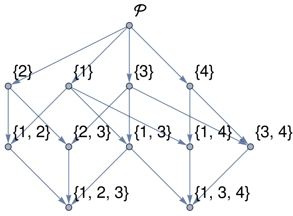
As an example, for one of the regions contributing to the graph , namely with the region vector , we find the divergent rays shown in the left panel of Fig. 2. These are the first integer vectors along the positive direction of the outward-pointing normal to a facet of the Newton polytope defined in Eq. (31). We listed only facets that are responsible for a pole in , i.e., such that . The subset of inducing higher order poles in is shown in its combinatorial structure in the right panel of Fig. 2. These are dual to the cones formed by taking a positive combination of compatible rays. Each node in the partially ordered set corresponds to a face of of co-dimension equal to the number of compatible rays. In particular, at the lower level of the partially ordered set, we find the cones responsible for the leading pole in . They are computed by means of the formula (33) from Salvatori:2024nva in terms of convergent integrals of the lowest dimension. Conversely, the top level of the diagram is a single integral of the highest dimension. Its integrand is the result of the renormalization map, described in Ref. Salvatori:2024nva , applied to the integrand (29). This is the only term in (33) that does not produce a pole in .
As a next step, we evaluated emerging locally finite integrals from the previous step by expanding their integrands in and integrating the series term-by-term using HyperInt of Panzer:2014gra . The algorithm devised in Panzer:2014gra integrates one variable at a time, expressing the result in terms of Goncharov polylogarithms. This works only for linearly reducible integrals, those for which there is at least one order of the integration variables where at each step the partial integral is a polylogarithmic function with rational prefactors such that both the letters and the poles of the prefactor are linear in the next integration variable. An appealing feature of this code is that it provides a way to safely ignore spurious divergent contributions appearing in intermediate integration steps with the use of the shuffle regularization. This means that if we know that an integral is convergent, even though the individual integrals are divergent, HyperInt is able to integrate each integrand separately while systematically dropping divergent terms. The latter are guaranteed to cancel when adding the two up together. The only restriction to this procedure is that both integrals must be calculated by integrating variables in the same order. Accordingly, in order to evaluate an integral of a locally finite integrand, written as a combination of Euler integrands in the same integration domain, we listed all the admissible integration orders for each of the individual integrands and then kept only those that are common.
In principle, HyperInt should be able to integrate locally finite integrands using any common order. However, different orders required very
different CPU times for the integrals to be carried over, with some simply never terminating. As a practical solution to this issue, we merely attempted
various orders simultaneously until we found one that terminated successfully.
With this strategy, we were able to evaluate all the contributions of regions for diagrams , , , , and . Among these, the regions , , and proved to be untractable by the Mellin-Barnes approach described in the previous section.
On the other hand, not all of the region integrals met the above criteria. For example, for the diagram the region with vector yields an integral whose divergent rays are depicted in Fig. 3.
The fourth divergent ray is compatible with all the others, and it belongs to their linear span, breaking the second criterion. Applying once a Nilsson-Passare analytical continuation Berkesch ; Nilsson along the fourth vector, we reduce the original integral to a combination of integrals satisfying the required criteria. In this manner, we can therefore calculate them individually with the same formula as before. The caveat is that we had to reach a higher order in the -expansion. Although we always find them to be linearly reducible, the sheer amount of integrands adds up quickly and becomes very time-consuming to be a practical strategy888To address this issue, we consider it highly desirable to develop a proper parallelization of core functionalities of HyperInt.. This issue was particularly severe for diagrams and , for which multiple regions broke the requirements necessary for the ‘subtraction’ formula. Luckily, the contributions of regions for proved tractable by the Mellin-Barnes approach, and the contributions of regions for were calculated with differential equations, so that every region was covered by at least one of the three methods.
5 Solving integrals with differential equations
We now return to the remaining, hard regions with -behavior. These are obtained from ab initio integrals by setting . Their integrands do not simplify sufficiently for to warrant using their parametric representations directly for subsequent calculations. Instead, it is much more efficient to reduce the original massless on-shell momentum integrals to a set of master integrals by means of integration-by-parts relations. These master integrals were calculated before Gehrmann:2006wg ; Heinrich:2007at ; Baikov:2009bg ; Heinrich:2009be and are available up to transcendentality weight eight from Ref. Lee:2010ik .
Finally, we needed to calculate contributions of individual regions for integrals that yielded multifold MB integrals that could not be tamed numerically with sufficient precision. All of them appeared in . Here again, we have applied the method of the differential equations Kotikov:1990kg ; Gehrmann:1999as ; Henn:2013pwa . In fact, this method was applied earlier to the three-loop massless vertex integrals Pikelner:2021goo at the so-called symmetrical point, i.e., . By adopting this earlier analysis in Belitsky:2023ssv , we evaluated our integrals at general values of and , with and then deduced results for their asymptotics by expanding the thus-obtained analytical results.
Presently, we need to evaluate, however, the contributions of individual regions for the leading order in the small- expansion of . As in the previous analysis, we start from differential equations at generic values of for the 77 primary master integrals. We introduce a new variable, i.e, , that rationalizes and, therefore, avoids potential square roots in resulting differential equations. Then turn to their canonical form Henn:2013pwa using the available public codes like, e.g., CANONICA Meyer:2017joq ,
| (35) |
Here is a vector of canonical basis elements and is a corresponding matrix with elements being functions of but independent of .
Since we only need the leading asymptotics of the 77 elements of the canonical basis in the limit , these can be extracted from the matrix exponent , where is the -coefficient of . The rest of the terms are irrelevant for our purposes. Matrix elements of this matrix exponent are linear combinations of the powers with . Here , , are the integration constants. They are uniformly-transcendental linear combinations of the form , where . Once these boundary conditions are fixed, we obtain the leading asymptotics of the elements of the canonical basis in the limit . Integration-by-parts identities provide us with a relation of to the found elements of the canonical basis in the limit . To fix , it was sufficient to apply explicit analytic solutions for the master integrals at general obtained in Pikelner:2021goo and then to expand corresponding expressions in the leading order of the limit .
In this manner, we deduced the Laurent expansion of contributions to all relevant regions up to . They are listed in Appendix A.3. A more detailed presentation of three-loop results is given in the accompanying ancillary files attached with this submission.
6 Factorization
Now we are in a position to assemble our findings in the three-loop form factor. Contributing graphs, enumerated according to the nomenclature of Fig. 1, at each consecutive -loop order, enter the Sudakov form factor with integer coefficients . was quoted in Eq. (8), so . For the rest, we have
| (36) |
with
| (37) |
Here, the two- and three-loop integrals are decomposed over contributing regions as
| (38) | ||||
| (39) | ||||
where we did not split collinear regions up further with respect to legs and . We can immediately verify the correctness of the total sum against Eq. (6), which was obtained solely on the basis of determining master integrals through the method of differential equations. Indeed, it confirms the exponentiation of the Sudakov form factor flawlessly.
Anticipating the hard-ultrasoft-collinear factorization, we write an ansatz for
| (40) |
where the hard , jet , and ultrasoft functions receive contributions solely from hard, collinear, and ultrasoft modes, respectively. Explicitly,
| (41) | ||||
| (42) | ||||
| (43) |
where from Eqs. (17) and (18). This form implies that all mixed contributions, such as for instance, , should arise from products of individual regions from lower loop order. This statement can be confirmed or rebutted with our explicit three-loop results.
6.1 Hard factorization
Let us begin this analysis with the mixed contributions involving at least one hard region. At two loops, it is not hard to check that
| (44) |
Analogously, we find at three loops
| (45) | |||
| (46) | |||
| (47) |
These relations prove the expected factorization of the hard region from the ones with ultrasoft-collinear modes up to three-loop order.
6.2 Ultrasoft-collinear factorization: a two-loop obstruction
We now turn to separating collinear from ultrasoft regions. A quick inspection shows, however, that it is broken starting from two loops. Namely,
| (48) |
and this implies that the alleged multiplicative factorization (40) is violated.
Let us zoom in on this ‘problematic’ region. Since the double ladder and cross ladder yield, up to an overall numerical factor, identical expressions for this region, i.e., , we can focus on just one of these integrals. We consider which reads
| (49) |
In the -ordering there are two identical contributions, i.e., and , defining the ultrasoft-collinear region. Again, it suffices to discuss just one, say, determined by the vector , which unambiguously specifies the IR scaling of the integrand’s propagators. Namely, according to IR counting rules (13), and behave as
| (50) |
and do not change their form since both terms in the light-cone decomposition scale the same way. The propagator admits the eikonal form
| (51) |
while and are ultrasoft in this region
| (52) |
Finally, possesses two additive contributions
| (53) |
To achieve the desired factorization of the ultrasoft from the collinear region, we would like to drop the second term, which entangles the two loop momenta. However, this is not justified since both of them provide parametrically leading-order effects according to the IR counting rules.
To unravel the effect of this intertwining, we calculate the ultrasoft loop first. To this end, we use the Schwinger-time representation for the ultrasoft propagators (52) and the ‘offending’ one (53), where we temporarily introduce ,
| (54) |
where we extracted the leading IR asymptotics in the denominator after the Fourier transform in . Next, integrating over is straightforward as well as after the rescaling . Finally, changing the integration variable to via the map , we get
| (55) |
We now see explicitly that the second term in the square bracket of the integrand is the obstruction for factorization. It cannot be ignored since, while its numerator is suppressed by , it gets enhancement from the -collinear kinematics of the denominator. It is easy to calculate the resulting -integral yielding a closed-form geometric series. However, we will not do it since the integral form is more appropriate for the subsequent evaluation of the -loop. It yields the following -exact expression
| (56) |
Its Laurent expansion coincides with the result obtained from the parametric integral to . Comparing it with the product of the one-loop expressions, we conclude that
| (57) |
This implies that by accounting for the mismatch factor in (48), it becomes
| (58) |
such that the multiplicative separation of the collinear and ultrasoft modes (40) can be mended by twisting the mode functions, along with a finite renormalization of the ’t Hooft coupling Belitsky:2024yag to this perturbative order. However, this does not seem to be possible already at three loops.
6.3 Broken ultrasoft-collinear factorization
Going to three loops, first, we need to re-inspect Eq. (47) since it contains a mixed two-loop region, which is not a part of the incoherent components (41), (42), and (43). But, we already know that it will be broken when is naively recast in terms of the product as was observed in Eq. (48). To save the day, it needs an adjustment factor. Indeed, it is the very same as in Eq. (58), so that Eq. (47) is superseded by
| (59) |
This is the harbinger of a problem. Now, the twisting implemented at two loops does not work since it produces a single factor of rather than the required in the simple, multiplicative factorization. Though replacing the product with a convolution could reproduce it, we will not dwell on it since further considerations of the remaining three-loop mixed regions involving only collinear and ultrasoft modes introduce irreparable complications in our attempt to separate them.
An inspection of both and regions demonstrates that they cannot simply be represented in terms of lower-loop incoherent components; instead, they require additional adjustment factors. With a little ingenuity, they can be found. The equations
| (60) | |||
| (61) |
hold to for
| (62) | ||||
| (63) |
Notice that the factorization breaking is postponed to order in the -factors when , determined at earlier loop order, is included. Unfortunately, and are different, which prevents us from twisting the two-loop incoherent components of and to accommodate this violation.
The inability to separate the collinear and ultrasoft regions necessitates a modification in Eq. (40) with a factorization-restoring factor
| (64) |
with
| (65) | ||||
and the -factors being
| (66) | ||||
| (67) |
Considering the fact that at each -th order of the perturbation theory, the Laurent series possesses the leading singularity , the breaking of the ultrasoft-collinear factorization is pushed to the subleading order . This is the order at which the violation first occurred at two loops, as was clarified in Sect. 6.2.
7 Conclusions
In this work, we considered factorization properties of the off-shell Sudakov form factor at higher orders of perturbative expansion. We observed that the hard factorization is valid, i.e., short-distance physics is indeed incoherent from the IR physics governing its near mass-shell behavior. However, we found a violation of the IR factorization for the collinear and ultrasoft modes. These remain entangled. It starts at two loops in subleading orders of the -expansion. It is unsettling that an IR-sensitive observable as simple as the Sudakov form factor defies traditional soft-collinear factorization. This appears to suggest that all on-shell scattering amplitudes on this Coulomb branch will follow suit. In this paper, we did not address the question of the operator definition for the joint ultrasoft-collinear functions. This could be of value, and our findings will be reported elsewhere.
Acknowledgements.
We are deeply indebted to Giulio Salvatori for a fruitful collaboration on this paper, which would not have been possible without his contribution. The implementation of his method was crucial Salvatori:2024nva for the completion of this project. We are grateful to Andrei Pikelner for providing details of the calculation reported in Ref. Pikelner:2021goo . The work of A.B. was supported by the U.S. National Science Foundation under grant No. PHY-2207138. The work of V.S. was conducted under the state assignment of Lomonosov Moscow State University and supported by the Moscow Center for Fundamental and Applied Mathematics of Lomonosov Moscow State University under Agreement No. 075-15-2025-345.Appendix A -expansion for regions
In this appendix, we present Laurent expansions for regions at one, two, and three loops. Whenever there is an exact result in , we quote it instead.
A.1 One loop
At one-loop, contributions of all regions can be evaluated as exact functions of :
| (68) | ||||
| (69) | ||||
| (70) |
A.2 Two loops
At two loops, the results are required to order compared to of Ref. Belitsky:2024yag . They are
| (71) | ||||
| (72) | ||||
| (73) | ||||
| (74) | ||||
| (75) | ||||
| (76) |
and
| (77) | ||||
| (78) | ||||
| (79) | ||||
| (80) | ||||
| (81) | ||||
| (82) |
A.3 Three loops
Finally, at three loops, the expansion was obtained to :
| (83) | ||||
| (84) | ||||
| (85) | ||||
| (86) | ||||
| (87) | ||||
| (88) | ||||
| (89) | ||||
| (90) | ||||
| (91) | ||||
| (92) |
for
| (93) | ||||
| (94) | ||||
| (95) | ||||
| (96) | ||||
| (97) | ||||
| (98) | ||||
| (99) | ||||
| (100) | ||||
| (101) | ||||
| (102) |
for
| (103) | ||||
| (104) | ||||
| (105) | ||||
| (106) | ||||
| (107) | ||||
| (108) | ||||
| (109) | ||||
| (110) | ||||
| (111) | ||||
| (112) |
for
| (113) | ||||
| (114) | ||||
| (115) | ||||
| (116) | ||||
| (117) | ||||
| (118) | ||||
| (119) | ||||
| (120) | ||||
| (121) | ||||
for
| (122) | ||||
| (123) | ||||
| (124) | ||||
| (125) | ||||
| (126) | ||||
| (127) | ||||
| (128) | ||||
| (129) | ||||
| (130) | ||||
| (131) | ||||
for the sum
| (132) | ||||
| (133) | ||||
| (134) | ||||
| (135) | ||||
| (136) | ||||
| (137) | ||||
| (138) | ||||
| (139) | ||||
| (140) | ||||
| (141) |
for , and finally
| (142) | ||||
| (143) | ||||
| (144) | ||||
| (145) | ||||
| (146) | ||||
| (147) | ||||
| (148) | ||||
| (149) | ||||
| (150) | ||||
| (151) |
for .
Mathematica-ready expressions for individual regions of the above three-loop results are given in the attached ancillary files.
References
- (1) V. V. Sudakov, Vertex parts at very high-energies in quantum electrodynamics, Sov. Phys. JETP 3 (1956) 65–71.
- (2) L. D. Landau, On analytic properties of vertex parts in quantum field theory, Nucl. Phys. 13 (1959) 181–192.
- (3) S. Coleman and R. E. Norton, Singularities in the physical region, Nuovo Cim. 38 (1965) 438–442.
- (4) A. Sen, Asymptotic Behavior of the Sudakov Form-Factor in QCD, Phys. Rev. D 24 (1981) 3281.
- (5) A. Sen, Asymptotic Behavior of the Wide Angle On-Shell Quark Scattering Amplitudes in Nonabelian Gauge Theories, Phys. Rev. D 28 (1983) 860.
- (6) J. C. Collins, D. E. Soper and G. F. Sterman, Factorization of Hard Processes in QCD, Adv. Ser. Direct. High Energy Phys. 5 (1989) 1–91, [hep-ph/0409313].
- (7) G. F. Sterman and M. E. Tejeda-Yeomans, Multiloop amplitudes and resummation, Phys. Lett. B 552 (2003) 48–56, [hep-ph/0210130].
- (8) S. M. Aybat, L. J. Dixon and G. F. Sterman, The Two-loop soft anomalous dimension matrix and resummation at next-to-next-to leading pole, Phys. Rev. D 74 (2006) 074004, [hep-ph/0607309].
- (9) L. J. Dixon, L. Magnea and G. F. Sterman, Universal structure of subleading infrared poles in gauge theory amplitudes, JHEP 08 (2008) 022, [0805.3515].
- (10) T. Becher and M. Neubert, On the Structure of Infrared Singularities of Gauge-Theory Amplitudes, JHEP 06 (2009) 081, [0903.1126].
- (11) N. Agarwal, L. Magnea, C. Signorile-Signorile and A. Tripathi, The infrared structure of perturbative gauge theories, Phys. Rept. 994 (2023) 1–120, [2112.07099].
- (12) C. W. Bauer, S. Fleming, D. Pirjol and I. W. Stewart, An Effective field theory for collinear and soft gluons: Heavy to light decays, Phys. Rev. D 63 (2001) 114020, [hep-ph/0011336].
- (13) M. Beneke, A. P. Chapovsky, M. Diehl and T. Feldmann, Soft collinear effective theory and heavy to light currents beyond leading power, Nucl. Phys. B 643 (2002) 431–476, [hep-ph/0206152].
- (14) T. Becher, A. Broggio and A. Ferroglia, Introduction to Soft-Collinear Effective Theory, vol. 896. Springer, 2015, 10.1007/978-3-319-14848-9.
- (15) I. Feige and M. D. Schwartz, An on-shell approach to factorization, Phys. Rev. D 88 (2013) 065021, [1306.6341].
- (16) I. Feige and M. D. Schwartz, Hard-Soft-Collinear Factorization to All Orders, Phys. Rev. D 90 (2014) 105020, [1403.6472].
- (17) J. C. Collins and G. F. Sterman, Soft Partons in QCD, Nucl. Phys. B 185 (1981) 172–188.
- (18) G. T. Bodwin, S. J. Brodsky and G. P. Lepage, Initial State Interactions and the Drell-Yan Process, Phys. Rev. Lett. 47 (1981) 1799.
- (19) J. C. Collins, D. E. Soper and G. F. Sterman, All Order Factorization for Drell-Yan Cross-sections, Phys. Lett. B 134 (1984) 263.
- (20) I. Z. Rothstein and I. W. Stewart, An Effective Field Theory for Forward Scattering and Factorization Violation, JHEP 08 (2016) 025, [1601.04695].
- (21) M. D. Schwartz, K. Yan and H. X. Zhu, Collinear factorization violation and effective field theory, Phys. Rev. D 96 (2017) 056005, [1703.08572].
- (22) J. C. Collins, D. E. Soper and G. F. Sterman, Soft Gluons and Factorization, Nucl. Phys. B 308 (1988) 833–856.
- (23) S. M. Aybat and G. F. Sterman, Soft-Gluon Cancellation, Phases and Factorization with Initial-State Partons, Phys. Lett. B 671 (2009) 46–50, [0811.0246].
- (24) M. D. Schwartz, K. Yan and H. X. Zhu, Factorization Violation and Scale Invariance, Phys. Rev. D 97 (2018) 096017, [1801.01138].
- (25) J. R. Forshaw, A. Kyrieleis and M. H. Seymour, Super-leading logarithms in non-global observables in QCD, JHEP 08 (2006) 059, [hep-ph/0604094].
- (26) T. Becher, M. Neubert and D. Y. Shao, Resummation of Super-Leading Logarithms, Phys. Rev. Lett. 127 (2021) 212002, [2107.01212].
- (27) P. Böer, P. Hager, M. Neubert, M. Stillger and X. Xu, Renormalization-group improved resummation of super-leading logarithms, JHEP 08 (2024) 035, [2405.05305].
- (28) S. Catani, D. de Florian and G. Rodrigo, Space-like (versus time-like) collinear limits in QCD: Is factorization violated?, JHEP 07 (2012) 026, [1112.4405].
- (29) J. R. Forshaw, M. H. Seymour and A. Siodmok, On the Breaking of Collinear Factorization in QCD, JHEP 11 (2012) 066, [1206.6363].
- (30) M. Beneke and V. A. Smirnov, Asymptotic expansion of Feynman integrals near threshold, Nucl. Phys. B 522 (1998) 321–344, [hep-ph/9711391].
- (31) V. A. Smirnov, Applied asymptotic expansions in momenta and masses, Springer Tracts Mod. Phys. 177 (2002) 1–262.
- (32) V. A. Smirnov, Analytic tools for Feynman integrals, Springer Tracts Mod. Phys. 250 (2012) 1–296.
- (33) V. A. Smirnov, Expansion by Regions: An Overview. 2021. 2406.11475.
- (34) A. V. Belitsky, L. V. Bork and V. A. Smirnov, Pinching Sudakov, 2409.05945.
- (35) T. Dennen, Y.-t. Huang and W. Siegel, Supertwistor space for 6D maximal super Yang-Mills, JHEP 04 (2010) 127, [0910.2688].
- (36) Z. Bern, J. J. Carrasco, T. Dennen, Y.-t. Huang and H. Ita, Generalized Unitarity and Six-Dimensional Helicity, Phys. Rev. D 83 (2011) 085022, [1010.0494].
- (37) A. V. Belitsky, Collinear anatomy, 2412.11886.
- (38) S. Caron-Huot and F. Coronado, Ten dimensional symmetry of = 4 SYM correlators, JHEP 03 (2022) 151, [2106.03892].
- (39) R. Jackiw, Dynamics at high momentum and the vertex function of spinor electrodynamics, Annals Phys. 48 (1968) 292–321.
- (40) W. L. van Neerven, Infrared Behavior of On-shell Form-factors in a Supersymmetric Yang-Mills Field Theory, Z. Phys. C 30 (1986) 595.
- (41) T. Gehrmann, J. M. Henn and T. Huber, The three-loop form factor in N=4 super Yang-Mills, JHEP 03 (2012) 101, [1112.4524].
- (42) L. F. Alday, J. M. Henn, J. Plefka and T. Schuster, Scattering into the fifth dimension of N=4 super Yang-Mills, JHEP 01 (2010) 077, [0908.0684].
- (43) A. V. Belitsky, L. V. Bork, A. F. Pikelner and V. A. Smirnov, Exact Off Shell Sudakov Form Factor in N=4 Supersymmetric Yang-Mills Theory, Phys. Rev. Lett. 130 (2023) 091605, [2209.09263].
- (44) A. V. Belitsky, L. V. Bork and V. A. Smirnov, Off-shell form factor in =4 sYM at three loops, JHEP 11 (2023) 111, [2306.16859].
- (45) J. M. Henn, Multiloop integrals in dimensional regularization made simple, Phys. Rev. Lett. 110 (2013) 251601, [1304.1806].
- (46) Z. Bern, L. J. Dixon, D. C. Dunbar and D. A. Kosower, Fusing gauge theory tree amplitudes into loop amplitudes, Nucl. Phys. B 435 (1995) 59–101, [hep-ph/9409265].
- (47) Z. Bern, L. J. Dixon, D. C. Dunbar and D. A. Kosower, One loop n point gauge theory amplitudes, unitarity and collinear limits, Nucl. Phys. B 425 (1994) 217–260, [hep-ph/9403226].
- (48) A. V. Belitsky and G. P. Korchemsky, Exact null octagon, JHEP 05 (2020) 070, [1907.13131].
- (49) T. Y. Semenova, A. V. Smirnov and V. A. Smirnov, On the status of expansion by regions, Eur. Phys. J. C 79 (2019) 136, [1809.04325].
- (50) V. A. Smirnov, Problems of the strategy of regions, Phys. Lett. B 465 (1999) 226–234, [hep-ph/9907471].
- (51) A. Pak and A. Smirnov, Geometric approach to asymptotic expansion of Feynman integrals, Eur. Phys. J. C 71 (2011) 1626, [1011.4863].
- (52) G. Salvatori, The Tropical Geometry of Subtraction Schemes, 2406.14606.
- (53) B. Jantzen, A. V. Smirnov and V. A. Smirnov, Expansion by regions: revealing potential and Glauber regions automatically, Eur. Phys. J. C 72 (2012) 2139, [1206.0546].
- (54) A. V. Belitsky and V. A. Smirnov, An off-shell Wilson loop, JHEP 04 (2023) 071, [2110.13206].
- (55) V. A. Smirnov and F. Wunder, Expansion by regions meets angular integrals, JHEP 08 (2024) 138, [2405.13120].
- (56) A. V. Smirnov, FIESTA 3: cluster-parallelizable multiloop numerical calculations in physical regions, Comput. Phys. Commun. 185 (2014) 2090–2100, [1312.3186].
- (57) A. V. Smirnov, N. D. Shapurov and L. I. Vysotsky, FIESTA5: Numerical high-performance Feynman integral evaluation, Comput. Phys. Commun. 277 (2022) 108386, [2110.11660].
- (58) H. Cheng and T. T. Wu, EXPANDING PROTONS: SCATTERING AT HIGH-ENERGIES. 1987.
- (59) A. V. Kotikov, Differential equations method: New technique for massive Feynman diagrams calculation, Phys. Lett. B 254 (1991) 158–164.
- (60) T. Gehrmann and E. Remiddi, Differential equations for two-loop four-point functions, Nucl. Phys. B 580 (2000) 485–518, [hep-ph/9912329].
- (61) A. V. Belitsky, A. V. Smirnov and V. A. Smirnov, MB tools reloaded, Nucl. Phys. B 986 (2023) 116067, [2211.00009].
- (62) M. Czakon, Automatized analytic continuation of Mellin-Barnes integrals, Comput. Phys. Commun. 175 (2006) 559–571, [hep-ph/0511200].
- (63) A. V. Smirnov and V. A. Smirnov, On the Resolution of Singularities of Multiple Mellin-Barnes Integrals, Eur. Phys. J. C 62 (2009) 445–449, [0901.0386].
- (64) J. B. Tausk, Nonplanar massless two loop Feynman diagrams with four on-shell legs, Phys. Lett. B 469 (1999) 225–234, [hep-ph/9909506].
- (65) V. A. Smirnov, Analytical result for dimensionally regularized massless on shell double box, Phys. Lett. B 460 (1999) 397–404, [hep-ph/9905323].
- (66) H. R. P. Ferguson, D. Bailey and S. Arno, Analysis of PSLQ, an integer relation finding algorithm, Math. Comput. 68 (1999) 351–369.
- (67) N. Arkani-Hamed, A. Hillman and S. Mizera, Feynman polytopes and the tropical geometry of UV and IR divergences, Phys. Rev. D 105 (2022) 125013, [2202.12296].
- (68) A. Hillman, On the Infrared and Ultraviolet Behavior of Scattering Amplitudes and Wavefunctions. PhD thesis, Princeton U., 2023.
- (69) C. Berkesch, J. Forsgård and M. Passare, Euler-mellin integrals and a-hypergeometric functions, Michigan Mathematical Journal 63 (Mar., 2014) 101–123.
- (70) L. Nilsson and M. Passare, Mellin transforms of multivariate rational functions, arXiv e-prints (Oct., 2010) arXiv:1010.5060, [1010.5060].
- (71) G. ’t Hooft and M. J. G. Veltman, Regularization and Renormalization of Gauge Fields, Nucl. Phys. B 44 (1972) 189–213.
- (72) E. Gawrilow and M. Joswig, polymake: a Framework for Analyzing Convex Polytopes. 2000. 10.1007/978-3-0348-8438-9-2.
- (73) E. Panzer, On hyperlogarithms and Feynman integrals with divergences and many scales, JHEP 03 (2014) 071, [1401.4361].
- (74) T. Gehrmann, G. Heinrich, T. Huber and C. Studerus, Master integrals for massless three-loop form-factors: One-loop and two-loop insertions, Phys. Lett. B 640 (2006) 252–259, [hep-ph/0607185].
- (75) G. Heinrich, T. Huber and D. Maitre, Master integrals for fermionic contributions to massless three-loop form-factors, Phys. Lett. B 662 (2008) 344–352, [0711.3590].
- (76) P. A. Baikov, K. G. Chetyrkin, A. V. Smirnov, V. A. Smirnov and M. Steinhauser, Quark and gluon form factors to three loops, Phys. Rev. Lett. 102 (2009) 212002, [0902.3519].
- (77) G. Heinrich, T. Huber, D. A. Kosower and V. A. Smirnov, Nine-Propagator Master Integrals for Massless Three-Loop Form Factors, Phys. Lett. B 678 (2009) 359–366, [0902.3512].
- (78) R. N. Lee and V. A. Smirnov, Analytic Epsilon Expansions of Master Integrals Corresponding to Massless Three-Loop Form Factors and Three-Loop g-2 up to Four-Loop Transcendentality Weight, JHEP 02 (2011) 102, [1010.1334].
- (79) A. Pikelner, Three-loop vertex integrals at symmetric point, JHEP 06 (2021) 083, [2104.06958].
- (80) C. Meyer, Algorithmic transformation of multi-loop master integrals to a canonical basis with CANONICA, Comput. Phys. Commun. 222 (2018) 295–312, [1705.06252].