GLAMP: An Approximate Message Passing Framework for Transfer Learning with Applications to Lasso-based Estimators

Abstract

Approximate Message Passing (AMP) algorithms enable precise characterization of certain classes of random objects in the high-dimensional limit, and have found widespread applications in fields such as statistics, deep learning, genetics, and communications. However, existing AMP frameworks cannot simultaneously handle matrix-valued iterates and non-separable denoising functions. This limitation prevents them from precisely characterizing estimators that draw information from multiple data sources with distribution shifts. In this work, we introduce Generalized Long Approximate Message Passing (GLAMP), a novel extension of AMP that addresses this limitation. We rigorously prove state evolution for GLAMP. GLAMP significantly broadens the scope of AMP, enabling the analysis of transfer learning estimators that were previously out of reach. We demonstrate the utility of GLAMP by precisely characterizing the risk of three Lasso-based transfer learning estimators: the Stacked Lasso [1], the Model Averaging Estimator [1], and the Second Step Estimator [2]. We also demonstrate the remarkable finite sample accuracy of our theory via extensive simulations.

1 Introduction

Transfer learning has emerged as a popular paradigm for handling distribution shifts between training and test time. In high-dimensional regression, substantial prior work has derived minimax error bounds demonstrating when auxiliary datasets allow to reduce estimation error and improve convergence rates in transfer learning [1, 3, 4, 5, 6, 7, 8, 9, 10, 11]. These error bounds are often conservative, derived for worst-case scenarios, and omit constant factors. Consequently, when applied in practice, the risks for transfer learning based estimators may differ vastly, making it difficult to perform realistic comparisons among estimators. This paper addresses this difficulty by introducing a novel approximate message passing framework for tracking the risks of Lasso-inspired estimators in transfer learning.

Specifically, we consider the proportional asymptotics regime, where the number of samples and features both diverge with the ratio converging to a constant. This regime has garnered significant attention in high-dimensional statistics and machine learning due to its ability to capture empirical phenomena in moderate to high-dimensional/overparametrized problems remarkably well [12, 13, 14, 15, 16, 17, 18, 19, 20, 21, 22, 23, 24, 25, 26, 27, 28, 29, 30, 31]. We introduce a new approximate message passing framework, coined generalized long AMP (GLAMP), that allows to characterize the risk of several transfer learning-based estimators. Concretely, we show the utility of our framework for the following three estimators: the Stacked Lasso [1], the Model Averaging estimator [1], and the Second-Step estimator [2]. To our knowledge, our paper provides the first general-purpose framework for characterizing the precise risks of these transfer learning-based estimators in high dimensions.

Approximate message passing algorithms were introduced in the compressed sensing literature [13] and have seen enormous success in quantifying the risks of convex regularized estimators in high dimensions [32, 33, 34, 16, 17, 21, 35, 36]. In its symmetric formulation, AMP takes as input a random design matrix $A\in\mathbb{R}^{N\times N}$, a sequence of deterministic separable functions $f_{t}:\mathbb{R}^{N}\rightarrow\mathbb{R}^{N}$, and generates a sequence of vectors $x^{t}\in\mathbb{R}^{N}$ in the following way:

$$x^{t+1}=Af_{t}(x^{t})-f_{t-1}(x^{t-1})B_{t}^{\top},$$

where $B_{t}$ has a specific form determined by the choice of the denoising functions $f_{t}$. Remarkably, AMP iterates admit precise characterizations: for each $t$, as $N\rightarrow\infty$, $x^{t}$ behaves as a Gaussian variable with a tractable variance, a property known as state evolution [37, 38]. For a broad range of statistical estimators, one can design suitable AMP iterations that track the estimator of interest (as $t$ additionally diverges to $\infty$), and thereby obtain exact risk characterization of these estimators. This is particularly useful for studying estimators without closed forms as demonstrated in [32, 33, 17], among others. Since its original introduction, the AMP framework has been extended to Generalized AMP (GAMP) [39, 40], which allows iteration on matrices $x^{t}\in\mathbb{R}^{N\times q}$, and Long AMP (LAMP) [41], which allows $f_{t}$ to be non-separable.

For our transfer learning scenario, none of the aforementioned formulations suffice. The challenge lies in tackling the distributions shifts among source and target distributions–no prior AMP framework allows to incorporate this. To mitigate this, we introduce Generalized Long AMP (GLAMP), which combines the strengths of Generalized AMP and Long AMP. GLAMP accommodates both matrix iterates $x^{t}\in\mathbb{R}^{N\times q}$ and non-separable functions $f_{t}$. Remarkably, this combination enables to track properties of estimators under distribution shifts. We establish rigorous state evolution results for GLAMP and show how it can be used to derive precise asymptotic risks for transfer learning estimators.

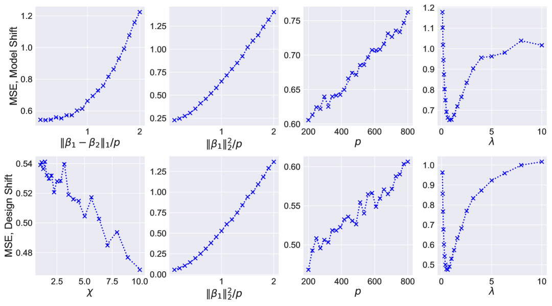
Figure 2: MSE for $\hat{\beta}_{\mathrm{average}}$. Same settings as in Figure 1.

To preview the utility of our framework, we describe our basic setting: we observe $E$ datasets $(y_{e},X_{e})$ with $y_{e}\in\mathbb{R}^{n_{e}},X_{e}\in\mathbb{R}^{n_{e}\times p}$ from potentially different distributions. Each dataset—referred to as an environment—follows a regression model with its own coefficient vector $\beta_{e}$ (see Assumption 2). The goal in transfer learning is to leverage information across these environments to improve the estimation of regression coefficients in a specific environment of interest. Multiple approaches have been proposed for this purpose, and we demonstrate the utility of GLAMP by analyzing three representative estimators: (i) Stacked Lasso [1], which serves as an early fusion method by combining all datasets at the start of learning. It solves an empirical risk minimization problem that takes a weighted aggregation of datasets with a usual lasso penalty; (ii) Model Averaging Estimator [1], which represents a late fusion approach by combining information at the end of learning. It computes individual lasso estimators from the environments and then takes their weighted average; (iii) Second-step estimator [2], which follows a pre-training and fine-tuning paradigm. It learns an initial estimator from all but the target environment, and then uses the target data to shrink the final estimator toward this initial one. To characterize the mean-squared error (MSE) of these estimators, one must account for both model and distribution shifts across environments. Traditional AMP frameworks have provided exact risk characterization of estimators based on data from a single distribution. In contrast, as we will show in Section 4, GLAMP can handle distribution shifts, enabling a unified analysis of diverse transfer learning methods. We further validate our theoretical results through extensive simulations (see Figures 1, 2, 3), demonstrating remarkable accuracy even in finite samples.

The rest of the paper is organized as follows. In Section 2, we provide a more comprehensive overview of related work in AMP and transfer learning. We formally introduce our symmetric GLAMP formulation in Section 3, and demonstrate its applicability for specific estimators in Section 4. In Section 5, we present asymmetric and multi-environment versions of GLAMP, two derivative formulations that are more directly related to our proofs. Finally, Section 6 outlines discussions and future directions.

Notations

We summarize below some notations used throughout the manuscript. Let $\|X\|_{2}$ denote the spectral norm of a matrix, and $\|v\|_{2}$ the Euclidean (or $\ell_{2}$) norm of a vector. More generally, $\|\cdot\|_{q}$ denotes the $\ell_{q}$ norm of a vector for $0\leq q\leq\infty$. For any set $A$, let $|A|$ denote its cardinality. Let $I_{p}$ be the $p\times p$ identity matrix, $\mathbb{E}[\cdot]$ the expectation operator, and $\mathbb{P}[\cdot]$ the probability of an event. For any positive definite matrix $\Sigma$, define $\|v\|_{\Sigma}=v^{\top}\Sigma v$ and $\langle v_{1},v_{2}\rangle_{\Sigma}=v_{1}^{\top}\Sigma v_{2}$. Moreover, we use $\lambda_{\max}(\Sigma)$ and $\lambda_{\min}(\Sigma)$ to denote the largest and smallest eigenvalues of the matrix $\Sigma$, respectively. For $v\in\mathbb{R}^{p}$, let $\operatorname{diag}(v)\in\mathbb{R}^{p\times p}$ denote the diagonal matrix with entries $[\operatorname{diag}(v)]_{i,j}=v_{j}\cdot\mathbf{1}\{i=j\}$. For any $m\in\mathbb{N}_{+}$, let $[m]=\{1,2,\dots,m\}$. Convergence in probability and in distribution are denoted by $\xrightarrow{p}$ and $\xrightarrow{d}$, respectively. We write $o_{\mathrm{P}}(1)$ for sequences of random variables converging to zero in probability.

2 Further Related Work

2.1 Approximate Message Passing

Approximate Message Passing (AMP) was first introduced in [13, 38]. Its origins can be traced back to the TAP equations from statistical physics [42, 37], and to loopy belief propagation from graphical models [43]. AMP has since achieved notable success in various statistical and applied domains such as linear regression [13, 38], generalized linear models [39, 17, 20], penalized regression [32, 44], low-rank matrix estimation [45], deep learning [46], and communications [47]. For a more comprehensive review, see [34, 35, 36] and the references therein.

On the technical front, the first rigorous state evolution analysis was provided in [38], relying on a crucial conditioning technique introduced in [37]. Subsequent generalizations have extended AMP in multiple directions, including extensions to right-rotationally-invariant random matrices [48, 49, 50] and finite sample analyses [51, 52]. More closely related to our work, Generalized AMP (GAMP) was introduced in [39, 40], which accommodates iterates of stacked vectors or matrices, while Long AMP (LAMP) proposed in [41] enables the use of non-separable denoising functions. Despite the existence of these individual threads, our GLAMP framework poses its own challenges, and requires its own state evolution proof, which we establish in this work. Furthermore, the fact that such a GLAMP framework can track risks of transfer learning-based estimators is a crucial observation on its own, noted for the first time in our paper.

2.2 Transfer Learning

Substantial prior work exists in transfer learning. For this literature review, we focus specifically on penalized estimators that aggregate data from multiple environments. In Section 4, we demonstrate the utility of our GLAMP framework for three representative estimators: Stacked Lasso, Model Averaging and Second-Step. However, the applicability of GLAMP extends beyond these examples. For instance, the methods proposed in [2, 10, 53], which are based on similar multi-stage estimation schemes, could be analyzed by adapting our approach for the Second-Step estimator. Likewise, the residual-weighting method from [54] can be studied using an analysis similar to that for the Stacked Lasso. Our framework can also accommodate penalties other than the vanilla Lasso, in the same way that AMP has been used to analyze a wide range of penalized procedures [55, 56] by selecting appropriate denoising functions $f_{t}$. This is particularly relevant for the transfer learning methods in [7, 57, 8], which rely on variants of the group Lasso. Finally, prior work has characterized the precise asymptotic risk of ridge-based transfer learning estimators using random matrix theory [58, 59, 60, 61, 62]. However, these arguments do not generalize beyond the ridge penalty or to settings where random matrix theory is inapplicable, such as the Lasso-based estimators that we study in this paper.

3 Generalized Long AMP

In this section, we introduce our symmetric GLAMP framework and relevant convergence results as a standalone contribution. For the transfer learning applications described in Section 4, generalized versions of this GLAMP framework—particularly asymmetric and multi-environment extensions—will be required. These generalizations are more complicated thus we defer their presentation to Section 5.

3.1 Setup

We first define pseudo-Lipschitz functions, which are used throughout the manuscript.

Definition 1 (Pseudo-Lipschitz functions).

For some fixed $q\in\mathbb{N}_{+}$ and fixed $k\in\mathbb{R},\,k\geq 1$:

1. We say a class of functions $\{\phi_{N}:(\mathbb{R}^{N})^{q}\to\mathbb{R}\}$ is uniformly pseudo-Lipschitz of order $k$ iff there exists some $L$ unrelated to $N$ such that $\forall\,x_{j},y_{j}\in\mathbb{R}^{N},j\in[q]$,

   $$\lvert\phi_{N}(x_{1},x_{2},\cdots,x_{q})-\phi_{N}(y_{1},y_{2},\cdots,y_{q})\rvert\leq L\left[1+\sum_{j\in[q]}\left(\frac{\lVert x_{j}\rVert_{2}}{\sqrt{N}}\right)^{k-1}+\sum_{j\in[q]}\left(\frac{\lVert y_{j}\rVert_{2}}{\sqrt{N}}\right)^{k-1}\right]\frac{\sum_{j\in[q]}\lVert x_{j}-y_{j}\rVert_{2}}{\sqrt{N}}.$$

2. We say a class of functions $\{\phi_{N}:\mathbb{R}^{N\times q}\to\mathbb{R}\}$ is uniformly pseudo-Lipschitz of order $k$ iff there exists some $L$ unrelated to $N$ such that $\forall\,X,Y\in\mathbb{R}^{N\times q}$ with spectral norms $\lVert X\rVert_{2},\lVert Y\rVert_{2},$

   $$\lvert\phi_{N}(X)-\phi_{N}(Y)\rvert\leq L\left[1+\left(\frac{\lVert X\rVert_{2}}{\sqrt{N}}\right)^{k-1}+\left(\frac{\lVert Y\rVert_{2}}{\sqrt{N}}\right)^{k-1}\right]\frac{\lVert X-Y\rVert_{2}}{\sqrt{N}}.$$

As a remark, Definition 1(a)–with a tuple of vectors as input–and 1(b)–with a matrix as input–are compatible. That is, if we write $X=[x_{1}|x_{2}|\cdots|x_{q}],Y=[y_{1}|y_{2}|\cdots|y_{q}],X,Y\in\mathbb{R}^{N\times q}$, then for any function sequence $\{\phi_{N}:(\mathbb{R}^{N})^{q}\to\mathbb{R}\}$ that is pseudo-Lipschitz by Definition 1(a), it is still uniformly pseudo-Lipschitz by Definition 1(b) when viewed as functions from $\mathbb{R}^{N\times q}\to\mathbb{R}$, and vice versa. This is because with fixed $q\in\mathbb{N}_{+}$, we have the matrix norm inequalities $\lVert X\rVert_{2}^{2}\leq\lVert X\rVert_{F}^{2}=\sum_{i\in[q]}\lVert x_{i}\rVert_{2}^{2}\leq q\cdot\lVert X\rVert_{2}^{2}$.

Now we are ready to officially define a symmetric GLAMP framework.

Definition 2 (Symmetric GLAMP Instance).

Let $q\in\mathbb{N}_{+}$ be fixed and known, and consider the asymptotic regime where $N\rightarrow\infty$. A symmetric GLAMP instance is a quadruple $\{A,(f_{t})_{t\in\mathbb{N}},x^{0},Y\}$, where $A\in\mathbb{R}^{N\times N}$ is a symmetric random design matrix, $Y\in\mathbb{R}^{N\times q}$ encodes information that the GLAMP iterates can use, $(f_{t})_{t\in\mathbb{N}}$ is a collection of mappings with $f_{t}:\mathbb{R}^{N\times q}\times\mathbb{R}^{N\times q}\to\mathbb{R}^{N\times q}$, and $x^{0}\in\mathbb{R}^{N\times q}$ is the initial condition for the GLAMP iterates.

The quadruple fully determines the GLAMP framework, and all subsequent iteration and convergence notations are defined based on this instance. Moreover, when $x^{0}$ and $Y$ are clear in a particular context, we sometimes only use $\{A,(f_{t})_{t\in\mathbb{N}}\}$ to denote the GLAMP instance. Similarly, as we will always take $Y$ as the second argument of $f_{t}$, we may simply write $f_{t}(\cdot)$ to denote $f_{t}(\cdot,Y)$.

We list the following assumptions accompanying the GLAMP instance:

Assumption 1 (Symmetric GLAMP assumptions).

With the GLAMP instance in Definition 2, we assume

1. $A=G+G^{{\top}}$ where $G\in\mathbb{R}^{N\times N}$ has iid Gaussian entries from $\mathcal{N}(0,\frac{1}{2N})$. This means $A$ is drawn from the Gaussian Orthogonal Ensemble (GOE) of dimension $N$, denoted as $A\sim\mathrm{GOE}(N)$.

2. $\limsup_{N}\frac{1}{N}\lVert Y\rVert_{2}^{2}<+\infty$.

3. $\limsup_{N}\frac{1}{N}\lVert x^{0}\rVert_{2}^{2}<+\infty$.

4. For each fixed $t\in\mathbb{N}$, $f_{t}$ is uniformly Lipschitz in $N$, in the sense that there exists some universal constant $L_{t}$ s.t. for any matrices $M_{1},M_{2},M_{1}^{\prime},M_{2}^{\prime}\in\mathbb{R}^{N\times q}$,

   $$\lVert f_{t}(M_{1},M_{2})-f_{t}(M_{1}^{\prime},M_{2}^{\prime})\rVert_{2}\leq L_{t}\lVert M_{1}-M_{1}^{\prime}\rVert_{2}+L_{t}\lVert M_{2}-M_{2}^{\prime}\rVert_{2},\ \forall\,N.$$

   Moreover, $\limsup_{N}\frac{1}{\sqrt{N}}\lVert f_{t}(0,0)\rVert_{2}<+\infty$.

5. Consider some fixed known $E\in\mathbb{N}_{+}$ and a sequence of $E$-partitions (groups) of $[N]$: $[N]=\cup_{a\in[E]}C_{a}^{N}$, and $\lim_{N\to\infty}\lvert C_{a}^{N}\rvert/N=c_{a}\in(0,1)$. For any step $t\in\mathbb{N}$, $f_{t}$ is separable among groups, in the sense that there are functions $g_{t,a}(\cdot,\cdot):\mathbb{R}^{\lvert C_{a}^{N}\rvert\times q}\times\mathbb{R}^{\lvert C_{a}^{N}\rvert\times q}\to\mathbb{R}^{\lvert C_{a}^{N}\rvert\times q}$ for each $a\in[E]$, s.t.

   $$f_{t}(x^{t},Y)=\begin{bmatrix}g_{t,1}(x^{t}_{C_{1}^{N}},Y_{C_{1}^{N}})\\ g_{t,2}(x^{t}_{C_{2}^{N}},Y_{C_{2}^{N}})\\ \vdots\\ g_{t,E}(x^{t}_{C_{E}^{N}},Y_{C_{p}^{N}})\end{bmatrix}.$$

6. If we write $q^{0}=f_{0}(x^{0})$, then $\forall\,a\in[E]$,

   $$\frac{1}{\lvert C_{a}^{N}\rvert}(q^{0}_{C_{a}^{N}})^{{\top}}q^{0}_{C_{a}^{N}}\to{\Sigma}_{a}^{0}$$

   for some matrices $\{{\Sigma}_{a}^{0}\in\mathbb{R}^{q\times q}:a\in[E]\}$. Specifically,

   $$\frac{1}{N}(q^{0})^{T}q^{0}\rightarrow\sum_{a\in E}c_{a}\Sigma_{a}^{0}:=\Sigma^{0}$$

7. For any constant covariance matrices $\Sigma_{1},\Sigma_{2}\in\mathbb{R}^{q\times q}$, any $s,r>0$ and any $a\in[E]$,

   $$\lim_{N\to\infty}\frac{1}{\lvert C_{a}^{N}\rvert}\mathbb{E}\left[g_{s,a}(Z_{1},Y_{C_{a}^{N}})^{{\top}}g_{r,a}(Z_{2},Y_{C_{a}^{N}})\right],\quad\lim_{N\to\infty}\frac{1}{\lvert C_{a}^{N}\rvert}\mathbb{E}\left[(q^{0}_{C_{a}^{N}})^{{\top}}g_{r,a}(Z_{2},Y_{C_{a}^{N}})\right]$$

   exist, where $Z_{1},Z_{2}\in\mathbb{R}^{\lvert C_{a}^{N}\rvert\times q}$ have iid row vectors from $\mathcal{N}(0,\Sigma_{1})$ and $\mathcal{N}(0,\Sigma_{2})$ respectively.

Given the instance in Definition 2, the symmetric GLAMP evolves according to the iterates defined below:

Definition 3 (Symmetric GLAMP Iterates).

We define the GLAMP iterates corresponding to an instance $\{A,(f_{t})_{t\in\mathbb{N}},x^{0},Y\}$ as the sequence of matrices $x^{t}\in\mathbb{R}^{N\times q}:t\in\mathbb{N}$ defined as follows:

$$x^{t+1}=Af_{t}(x^{t})-f_{t-1}(x^{t-1})B_{t}^{{\top}},\ {B}_{t}=\mathbb{E}\left[\frac{1}{N}\left(\sum_{j\in[N]}\frac{\partial(f_{t})_{j,\cdot}}{\partial x_{j,\cdot}}\right)(Z^{t})\right],$$ (1)

where $Z^{t}\in\mathbb{R}^{N\times q}$ has its rows drawn iid from $\mathcal{N}(0,\Sigma^{t})$ with $\Sigma^{t}$ to be defined. The term ${B}_{t}$ is understood as the average of $N$ Jacobians. As $f_{t}:\mathbb{R}^{N\times q}\to\mathbb{R}^{N\times q}$, $\frac{\partial(f_{t})_{j,\cdot}}{\partial x_{j,\cdot}}$ takes the $j$-th row of $f_{t}(\cdot)$ as a vector function, and consider its Jacobian only w.r.t. the $j$-th row of the input $x^{t}$.

As in prior work, $f_{t-1}(x_{t-1})B_{t}^{{\top}}$ is here the “Onsager term”. Accompanying the main GLAMP iterates on $x^{t}$, we also have the iterates on $\Sigma^{t}$ evolve as follows:

Definition 4 (Symmetric GLAMP State Evolution).

Starting from $\Sigma^{0}$ in Assumption 1(f), we define a sequence of matrices for ($t\in\mathbb{N}$):

$$\Sigma^{t+1}=\lim_{N\to\infty}\frac{1}{N}\mathbb{E}\left[f_{t}(Z^{t},Y)^{{\top}}f_{t}(Z^{t},Y)\right],$$

where $Z^{t}\in\mathbb{R}^{N\times q}$ has iid row vectors drawn from $\mathcal{N}(0,\Sigma^{t})$.

The state evolution defines a sequence of covariance structures that GLAMP iterates converge to, as will be formalized in our main result below.

3.2 Main Result

Theorem 1 (Symmetric GLAMP convergence).

Under Assumption 1, for any $t\in\mathbb{N_{+}}$ and any sequence of uniformly order-$k$ pseudo-Lipschitz functions $\phi_{N}:\mathbb{R}^{|C_{a}^{N}|\times(3q)}\to\mathbb{R}$ for any $k\geq 1$, the GLAMP iterates in Definition 3 satisfy:

$$\forall\,a\in[E],\ \phi_{N}([x^{0}_{C_{a}^{N}}|Y_{C_{a}^{N}}|x^{t}_{C_{a}^{N}}])=\mathbb{E}\left[\phi_{N}(x^{0}_{C_{a}^{N}}|Y_{C_{a}^{N}}|Z^{t}_{a})\right]+o_{\mathsf{P}}(1),$$

where $Z^{t}_{a}\in\mathbb{R}^{\lvert C_{a}^{N}\rvert\times q}$ has its row vectors drawn iid from $\mathcal{N}(0,\Sigma^{t})$ and $o_{\mathsf{P}}(1)$ denotes negligible in probability terms as $N\rightarrow\infty.$

Theorem 1 is the main result of this paper, and its proof is done in two steps, detailed in Section A.2 and Section A.3, respectively. At the end of Section A.3, we prove a slightly stronger Theorem A.2, which trivially implies Theorem 1.

The symmetric GLAMP framework is typically linked to statistical estimators in the following manner: $A$ is related to the design matrix, $Y$ to the response variable, and $(f_{t})_{t\in\mathbb{N}}$ to the specific estimator of interest. With proper initialization $x^{0}$ and under suitable conditions, taking $t\rightarrow\infty$ additionally above the $N\rightarrow\infty$ asymptotics in Theorem 1, the GLAMP instance converges to some $x^{\infty}$ that corresponds to our statistical estimator of interest. However, our end goal here is to study estimators under transfer learning where data from different distributions/environments are available. To study such estimators, two extensions of the symmetric GLAMP framework are necessary: asymmetric GLAMP (Section 5.1) and multi-environment GLAMP (Section 5.2). Introducing them requires more notation, thus instead of doing so, we first present applications of GLAMP to transfer learning.

4 Applications to Transfer Learning

We demonstrate the utility of GLAMP by investigating a class of Lasso-based estimators introduced in the transfer learning literature. We first define our transfer learning setting formally. We consider the problem where at training time data from multiple distributions are available—we call these the environments.

Assumption 2 (Transfer learning model).

Suppose there are $E\in\mathbb{N}_{+}$ environments, and consider for each $e\in E$, a sequence of problem instances $\{y_{e}(n_{e}),X_{e}(n_{e}),\beta_{e}(n_{e}),w_{e}(n_{e})\}$ with $y_{e}(n_{e})\in\mathbb{R}^{n_{e}}$, $X_{e}(n_{e})\in\mathbb{R}^{n_{e}\times p}$, $\beta_{e}(n_{e})\in\mathbb{R}^{p},w_{e}\in\mathbb{R}^{n_{e}}$ the response vector, the design matrix, the true regression coefficient and the noise, respectively. Further, we assume that $p,n_{e}\rightarrow\infty$, $\lim_{p\to\infty}p/n_{e}=\kappa_{e}\in(0,+\infty)$. In the sequel we will drop the dependence on $n_{e}$ for simplicity.

1. $\forall\,e\in[E]$, we assume a linear data generative model: $y_{e}=X_{e}\beta_{e}+w_{e}$, where $y_{e}\in\mathbb{R}^{n_{e}}$, $X_{e}\in\mathbb{R}^{n_{e}\times p}$, $\beta_{e}\in\mathbb{R}^{p},w_{e}\in\mathbb{R}^{n_{e}}$.

2. $X_{e}={X_{e}^{\mathrm{iid}}}\Sigma_{e}^{1/2}$, where $({X_{e}^{\mathrm{iid}}})_{i,j}\stackrel{{\scriptstyle\mathrm{iid}}}{{\sim}}\mathcal{N}(0,\frac{1}{n_{e}})$ are also independent across the environments. $\{\Sigma_{e}\}$ are deterministic, and $\exists\,c_{1}>1$ s.t. $c_{1}^{-1}\leq\inf_{p}\{\lambda_{\min}(\Sigma_{e})\}\leq\sup_{p}\{\lambda_{\max}(\Sigma_{e})\}\leq c_{1},\,\forall\,e\in[E]$.

3. $\sup_{e\in[E]}\limsup_{p}\frac{1}{p}\lVert\beta_{e}\rVert_{2}^{2}\leq+\infty$, and $\forall\,e\in[E]$, $\lim_{p}\frac{1}{p}\beta_{e}^{{\top}}\Sigma_{e}\beta_{e}$ exists.

4. The empirical distribution of $w_{e}$ converges in 2-Wasserstein distance to $W_{e}$, with $\mathbb{E}[W_{e}]=0$, $\mathbb{E}[W_{e}^{2}]<+\infty$.

Some comments are in order regarding the assumptions. Although Assumption 2(a) operates under linear models, we expect our GLAMP framework to be useful beyond this stylistic setting in the same way as GAMP served useful for non-linear models, c.f. [17, 20]. In Assumption 2(d), convergence in 2-Wasserstein distance is equivalent to requiring that the empirical distribution of $w_{e}$ converges to $W_{e}$ not only in distribution, but also in the first and second moments. In our formulation, as detailed in Assumption 2, we directly work with a deterministic sequence of $\{w_{e}\}$ and $\{\beta_{e}\}$. If they are sampled from a distribution, it must be independent from the design matrices or $\{{X_{e}^{\mathrm{iid}}}:e\in[E]\}$, so that conditioning on them does not effect the Gaussianity required for GLAMP. Beyond this independence requirement, GLAMP is sufficiently general to accommodate any correlation or dependence among these sequences, provided that the realized sequences for $\{w_{e}\}$ and $\{\beta_{e}\}$ satisfy Assumption 2(c), (d).

With the transfer learning setting defined, we investigate three estimators from the previous literature, and use the GLAMP framework to characterize their asymptotic risk under suitable conditions.

4.1 The Stacked Lasso

We begin with the stacked Lasso estimator–also known as the weighted loss estimator [1]–which is constructed by running the Lasso on the $E$ datasets stacked together, with different weights. In the hope that the analysis of the stacked Lasso will serve as a foundation for other estimators, we study a slightly generalized version that allows heterogeneous penalties across variables. Suppose we are given a deterministic sequence $\{\vec{\lambda}:\vec{\lambda}\in\mathbb{R}^{p},p\in\mathbb{N}\}$, and the penalty is defined as $\lVert\operatorname{diag}(\vec{\lambda})b\rVert_{1}=\sum_{j\in[p]}\vec{\lambda}_{j}\lvert b\rvert_{j}$ for any candidate $b\in\mathbb{R}^{p}$. The estimator $\hat{\beta}_{\mathrm{stack}}$ is then defined as:

$$\hat{\beta}_{\mathrm{stack}}=\operatorname*{\mathrm{argmin}}_{b\in\mathbb{R}^{p}}\mathcal{L}(b),\quad\mathcal{L}(b)=\frac{1}{2}\sum_{e\in[E]}\pi_{e}\left\lVert y_{e}-{X_{e}^{\mathrm{iid}}}\Sigma_{e}^{1/2}b\right\rVert_{2}^{2}+\left\lVert\operatorname{diag}(\vec{\lambda})b\right\rVert_{1}.$$ (2)

The coefficients $\{\pi_{e}:e\in[E]\}$ represent the weights assigned to each environment. We naturally assume that $\pi_{e}\geq 0,\,\forall\,e\in[E]$ and $\max\{\pi_{e}:e\in[E]\}>0$.

The stacked Lasso estimator in (2) depends on the random quantities $\{X_{e}\},\{y_{e}\}$. To capture its limiting behavior using GLAMP, we define a “fixed-design” counterpart function $\eta:(\mathbb{R}^{p})^{E}\to\mathbb{R}^{p}$ as follows:

$$\forall\,v_{1},\cdots,v_{E}\in\mathbb{R}^{p},\,\eta(v_{1},\cdots,v_{E})= ~\operatorname*{\mathrm{argmin}}_{b\in\mathbb{R}^{p}}\left\{\frac{1}{2}\sum_{e}\varpi_{e}\left\lVert\Sigma_{e}^{1/2}b-(v_{e}+\Sigma_{e}^{1/2}\beta_{e})\right\rVert_{2}^{2}+\theta\cdot\left\lVert\operatorname{diag}(\vec{\lambda})b\right\rVert_{1}\right\}.$$ (3)

By definition, $\eta$ depends on the covariances $\Sigma_{e}$, the true signals $\{\beta_{e}\}$, as well as $E+1$ deterministic (but yet to be defined) parameters $\theta$ and $\{\varpi_{e}\}$.

We need the following weak assumptions for the regularity of the stacked Lasso estimator:

Assumption 3 (Stacked Lasso GLAMP regularity).

Consider the transfer learning setting in Assumption 2, the stacked Lasso estimator in (2) and its fixed-design counterpart in (3).

1. $\liminf_{p}\min\{\vec{\lambda}_{j}:j\in[p]\}>0$, and $\limsup_{p}\frac{1}{p}\lVert\vec{\lambda}\rVert_{2}^{2}<+\infty$.

2. Define the following intermediate quantity

   $$\overline{\eta}=\overline{\eta}(\tau_{1},\tau_{2},\cdots,\tau_{E})=\eta(\tau_{1}Z_{1},\tau_{2}Z_{2},\cdots,\tau_{E}Z_{E}),$$ (4)

   for $\tau_{1},\tau_{2},\cdots,\tau_{E}>0$ and $Z_{1},Z_{2},\cdots,Z_{E}\stackrel{{\scriptstyle\mathrm{iid}}}{{\sim}}\mathcal{N}(0,I_{p})$. We assume $\forall\,\tau_{1},\tau_{2},\cdots,\tau_{E}>0$, $\theta>0$, $\varpi_{e}>0$ and $\sum_{e}\varpi_{e}=1$, the following limits exist: $\lim_{p}\frac{1}{p}\mathbb{E}[\lVert\overline{\eta}\rVert_{\Sigma_{e}}^{2}]$, $\lim_{p}\frac{1}{p}\mathbb{E}[\langle\beta_{e},\overline{\eta}\rangle_{\Sigma_{e}}]$, $\forall\,e\in[E]$.

3. Define the following intermediate quantity

   $$\mathcal{E}^{(p)}(\tau_{1},\cdots,\tau_{E})=\frac{1}{p}\mathbb{E}\left[\min_{b\in\mathbb{R}^{p}}\left\{\frac{1}{2}\sum_{e\in[E]}\varpi_{e}\left\lVert\Sigma_{e}^{1/2}b-(\tau_{e}Z_{e}+\Sigma_{e}^{1/2}\beta_{e})\right\rVert_{2}^{2}+\theta\left\lVert\operatorname{diag}{(\vec{\lambda})}b\right\rVert_{1}\right\}\right].$$ (5)

   We assume $\forall\,\tau_{1},\tau_{2},\cdots,\tau_{E}>0$, $\theta>0$, $\varpi_{e}>0$ and $\sum_{e}\varpi_{e}=1$, there exists a function $\mathcal{E}(\tau_{1},\cdots,\tau_{E})\in C^{1}$, s.t. $\lim_{p}\mathcal{E}^{(p)}=\mathcal{E}$, $\lim_{p}\frac{\partial}{\partial\tau_{e}}\mathcal{E}^{(p)}=\frac{\partial}{\partial\tau_{e}}\mathcal{E}$.

Assumption 3(b) makes sure the GLAMP iterates corresponding to the stacked Lasso have well-defined asymptotic limit, and Assumption 3(c) guarantees the well-definedness of the Onsager term, as demonstrated by the following result:

Proposition 1.

Under Assumptions 2, and 3, denote $\overline{\delta}_{e}^{{(p)}}:=\frac{1}{\tau_{e}p}\mathbb{E}\left[Z_{e}^{{\top}}\Sigma_{e}^{1/2}\overline{\eta}(\tau_{1},\tau_{2},\cdots,\tau_{E})\right]$, and let $S\subset[p]$ be the support of $\overline{\eta}\in\mathbb{R}^{p}$. Then we have the following equivalent forms of $\overline{\delta}^{{(p)}}_{e}$:

$$\overline{\delta}_{e}^{{(p)}}= ~\frac{1}{p}\sum_{j\in[p]}\mathbb{E}\left[\frac{\partial(\Sigma_{e}^{1/2}{\eta})_{j}}{\partial(\tau_{e}Z_{e})_{j}}(\tau_{1}Z_{1},\tau_{2}Z_{2},\cdots,\tau_{E}Z_{E})\right]$$ (6)

$$= ~\frac{1}{p}\mathbb{E}\left[\mathop{\mathrm{tr}}\left(\frac{\partial\eta}{\partial(\tau_{e}Z_{e})}(\tau_{1}Z_{1},\tau_{2}Z_{2},\cdots,\tau_{E}Z_{E})\Sigma_{e}^{1/2}\right)\right]$$

$$= ~\varpi_{e}\cdot\frac{1}{p}\mathbb{E}\left[\mathop{\mathrm{tr}}\bigg{(}\bigg{[}\sum_{e\in[E]}\varpi_{e}(\Sigma_{e})_{S,S}\bigg{]}^{-1}(\Sigma_{e})_{S,S}\bigg{)}\right].$$

Moreover, $\overline{\delta}_{e}:=\lim_{p}\overline{\delta}_{e}^{{(p)}}=\frac{1}{\tau_{e}}\lim_{p}\frac{1}{p}\mathbb{E}\left[Z_{e}^{{\top}}\Sigma_{e}^{1/2}\overline{\eta}(\tau_{1},\tau_{2},\cdots,\tau_{E})\right]$ is a well-defined limit. We have $\frac{1}{p}\mathbb{E}[\lVert\overline{\eta}(\tau_{1},\tau_{2},\cdots,\tau_{E})\rVert_{0}]=\sum_{e\in[E]}\overline{\delta}^{(p)}_{e}$ and $\lim_{p}\frac{1}{p}\mathbb{E}[\lVert\overline{\eta}(\tau_{1},\tau_{2},\cdots,\tau_{E})\rVert_{0}]=\sum_{e\in[E]}\overline{\delta}_{e}$.

Proposition 1 is proved in Appendix Section B.1.

Under Assumptions 2 and 3, we can track the asymptotic convergence of the corresponding GLAMP iterates (see Lemma C.2). We are left with one final piece: ensuring that the corresponding GLAMP indeed tracks the behavior of the stacked Lasso estimator. For that, we require the following assumption:

Assumption 4 (Stacked Lasso GLAMP fixed point).

Consider the transfer learning setting in Assumption 2, the stacked Lasso estimator in (2) and its fixed-design counterpart in (3).

1. There exist a $(2E+1)$-tuple $(\tau_{1}^{*},\cdots,\tau_{E}^{*},\varpi^{*}_{1},\cdots,\varpi^{*}_{E},\theta^{*})$ with $\theta^{*}>0$, $\tau^{*}_{e}>0$, and $\varpi^{*}_{e}\geq 0\ \forall\,e\in[E]$, which solves the following system of $(2E+1)$ equations:

   $$\begin{cases}\tau_{e}^{2}=\mathbb{E}[W_{e}^{2}]+\kappa_{e}\lim_{p}\frac{1}{p}\mathbb{E}\left[\left\lVert(\overline{\eta}-\beta_{e})\right\rVert_{\Sigma_{e}}^{2}\right],\ \forall\,e\in[E],\\ \pi_{e}\theta=\varpi_{e}/(1-\kappa_{e}\overline{\delta}_{e}),\ \forall\,e\in[E],\\ \sum_{e\in[E]}\varpi_{e}=1,\end{cases}$$ (7)

   where $\overline{\eta}$ from Equation (4) and $\{\overline{\delta}_{e}\}$ from Proposition 1 are all functions of the unknown variables.

2. For the $(\tau_{1}^{*},\cdots,\tau_{E}^{*},\varpi^{*}_{1},\cdots,\varpi^{*}_{E},\theta^{*})$ assumed to exist in Assumption 4(a), we define a function $H^{{(p)}}:[0,1]^{E}\to[0,1]^{E}$, whose $e$-th element $H_{e}^{(p)}$ is defined as:

   $$\forall\,\rho\in[0,1]^{E}, ~H^{(p)}_{e}(\rho)=H^{(p)}_{e}(\rho_{1},\rho_{2},\cdots,\rho_{E})=\frac{1}{(\tau_{e}^{*})^{2}}\left\{\mathbb{E}[W_{e}^{2}]+\frac{\kappa_{e}}{p}\mathbb{E}\left[\langle\overline{\eta}_{{(1)}}-\beta_{e},\overline{\eta}_{{(2)}}-\beta_{e}\rangle_{\Sigma_{e}}\right]\right\},$$ (8)

   where $\overline{\eta}_{{(1)}}=\eta(\tau^{*}_{1}Z_{1},\tau^{*}_{2}Z_{2},\cdots,\tau^{*}_{E}Z_{E})$, $\overline{\eta}_{{(2)}}=\eta(\tau^{*}_{1}Z_{1}^{\prime},\tau^{*}_{2}Z_{2}^{\prime},\cdots,\tau^{*}_{E}Z_{E}^{\prime})$, and the Gaussian variables involved satiesfy: (i) $Z_{e},Z^{\prime}_{e}$ are jointly normal, $Z_{e},Z^{\prime}_{e}\sim\mathcal{N}(0,I_{p})$ and $\mathop{\mathrm{cov}}(Z_{e},Z^{\prime}_{e})=\rho_{e}I_{p}$; (ii) The $E$ pairs of random variables $(Z_{e},Z^{\prime}_{e}),e=1,2,\cdots E$ are jointly independent. Further, we assume $H^{(p)}$ converges pointwise to some function $H:[0,1]^{E}\to[0,1]^{E}$ as $p\to+\infty$ with $H\in C^{1}$, and the convergence holds for all the partial derivatives, i.e. $\lim_{p}\frac{\partial H_{e}^{{(p)}}}{\partial\rho_{i}}=\frac{\partial H_{e}}{\partial\rho_{i}}$, $\forall\,e,i\in[E]$.

To connect Assumption 4 with the stacked Lasso, note that Assumption 4(a) establishes the existence of a fixed point for the GLAMP iterates that corresponds to the loss function from Equation (2), while Assumption 4(b) guarantees that the GLAMP iterates converge to that fixed point. Together, these two assumptions guarantee that the GLAMP iterates converge to a fixed point that asymptotically tracks $\hat{\beta}_{\mathrm{stack}}$.

With all assumptions in place, we state our main convergence result for $\hat{\beta}_{\mathrm{stack}}$.

Theorem 1 (Stacked Lasso convergence).

Under Assumptions 2,3 and 4, suppose we fix $\tau_{e}=\tau_{e}^{*}$, $\varpi_{e}=\varpi_{e}^{*}$, and $\theta=\theta^{*}$ in the definition of $\overline{\eta}$. Then, for any sequence of order-$k$ pseudo-Lipschitz functions $\phi:(\mathbb{R}^{p})^{E+1}\to\mathbb{R}$ with $k\geq 1$, we have

$$\phi\left(\hat{\beta}_{\mathrm{stack}},\beta_{1},\cdots,\beta_{E}\right)=\mathbb{E}\left[\phi(\overline{\eta}(\tau_{1}^{*},\tau_{2}^{*},\cdots,\tau_{E}^{*}),\beta_{1},\beta_{2},\cdots,\beta_{E})\right]+o_{\mathsf{P}}(1).$$

Theorem 1 is proved in Appendix Section C.

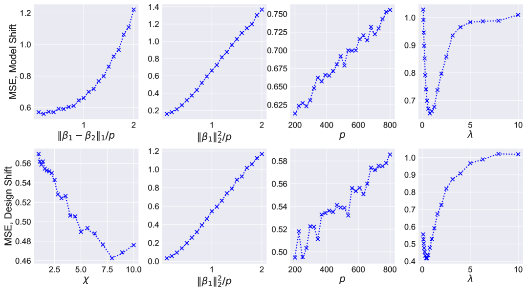
Figure 1: MSE of $\hat{\beta}_{\mathrm{stack}}$ under different scenarios. The dotted line indicates the theoretical MSE value obtained from our formulae while the cross marks indicate empirical MSE values. Base setting: $E=2$ (with $1$ as the target environment), $n_{1}=800$, $n_{2}=600$, $p=400$, $\Sigma_{1}=\Sigma_{2}=I$, $\beta_{1,j}=\beta_{2,j}\stackrel{{\scriptstyle\mathrm{iid}}}{{\sim}}\mathcal{N}(0,\sigma_{\beta}^{2})$ with $\sigma_{\beta}^{2}=1$, $w_{e,i}\stackrel{{\scriptstyle\mathrm{iid}}}{{\sim}}\mathcal{N}(0,\sigma_{w}^{2})$, $\sigma_{w}^{2}=1$, $\vec{\lambda}_{j}=1$, $\pi_{1}=\pi_{2}=1/2$. For model shift (the first row), $\beta_{2}=\beta_{1}+\tilde{\beta}$ with $\tilde{\beta}_{j}\stackrel{{\scriptstyle\mathrm{iid}}}{{\sim}}\mathcal{N}(0,\tilde{\sigma}^{2}\pi/2),\tilde{\sigma}^{2}=1$, while $\beta_{1}$ is taken to be as in the base setting. For design shift (the second row), $\Sigma_{2}$ differs from the base setting and is taken to be a diagonal matrix with two distinct eigenvalues $\chi,1/\chi$ that have equal multiplicity $p/2$. For each subplot, we change the parameter on the x-axis as shown, fixing others to follow the base setting. Note the remarkable alignment of the theoretical versus empirical values.

We demonstrate the finite-sample accuracy of the asymptotic convergence through numerical examples, with results presented in Figure 1. Specifically, we consider the case with $E=2$ environments. In the base setting, we set the sample sizes to $n_{1}=800$, $n_{2}=600$, and the feature dimension to $p=400$. The design matrices are isotropic with $\Sigma_{1}=\Sigma_{2}=I$. The signal vectors are generated as $\beta_{1,j}=\beta_{2,j}\overset{\text{i.i.d.}}{\sim}\mathcal{N}(0,\sigma_{\beta}^{2})$ for all $j\in[p]$, with $\sigma_{\beta}^{2}=1$, and the noise terms follow $w_{e,i}\overset{\text{i.i.d.}}{\sim}\mathcal{N}(0,\sigma_{w}^{2})$ for all $e\in[E]$, $i\in[n_{e}]$, with $\sigma_{w}^{2}=1$. We use a homogeneous regularization parameter $\vec{\lambda}$ with $\lambda=1$, and assign equal weights $\pi_{1}=\pi_{2}=1/2$. Building on this base case, we consider two types of transfer learning settings:

• Design/Covariate Shift: The underlying signal remains the same across environments as in the base setting, but the design matrix covariances differ. Specifically, we fix $\Sigma_{1}=I$ and set $\Sigma_{2}$ to be a diagonal matrix with two distinct eigenvalues $\chi$ and $1/\chi$, each with multiplicity $p/2$.

• Model/Signal Shift: The design matrix covariances remain the same as in the base setting, but the underlying signals differ. Specifically, we set $\beta_{2}=\beta_{1}+\tilde{\beta}$, where $\tilde{\beta}_{j}\overset{\text{i.i.d.}}{\sim}\mathcal{N}(0,\tilde{\sigma}^{2}\pi/2)$, such that $\|\tilde{\beta}\|_{1}/p\to\tilde{\sigma}^{2}$, while $\beta_{1}$ is taken to be as in the base setting.

In each setting, we vary different hyperparameter values and record the mean squared error (MSE) of the stacked Lasso estimator, defined as $\|\hat{\beta}_{\mathrm{stack}}-\beta_{1}\|_{2}^{2}$. Since our formulation assumes fixed signals, we draw a single realization of the signal vector for each experiment. We then perform $R=20$ independent realizations of the random design matrices $\{X_{e}\}$ and noise vectors $\{w_{e}\}$, along with $R=400$ realizations of $\{Z_{e}\}$ from Equation (4), to approximate the expectation.

Figure 1 confirms the remarkable finite-sample accuracy of Theorem 1, while also revealing several interesting trends. For example, the U-shaped curve with respect to changes in $\lambda$ suggests the potential effectiveness of adaptive tuning procedures. Additionally, the observation that the MSE decreases as $\chi$ increases indicates that heterogeneity across environments can be beneficial—an effect also noted by [60]. A more comprehensive study of the MSE and generalization error—which could provide further insights into estimator selection, data pooling strategies, and hyperparameter tuning—is left for future work.

4.2 The Model Averaging Estimator

Another straightforward approach to aggregating information from $E$ environments is to post-combine $E$ individual estimators via a weighted average. This method is known as the model averaging estimator [1]:

$$\hat{\beta}_{e}= ~\operatorname*{\mathrm{argmin}}_{b\in\mathbb{R}^{p}}L_{e}(b),\quad L_{e}(b)=\frac{1}{2}\left\|y_{e}-{X_{e}^{\mathrm{iid}}}\Sigma_{e}^{1/2}b\right\|_{2}^{2}+\left\|\operatorname{diag}(\vec{\lambda}_{e})b\right\|_{1},$$ (9)

$$\hat{\beta}_{\mathrm{average}}= ~\sum_{e\in[E]}\pi_{e}\hat{\beta}_{e},\quad\text{where }\sum_{e\in[E]}\pi_{e}=1.$$ (10)

For the single-environment Lasso estimator $\hat{\beta}_{e}$ defined in Equation (9), we adopt a heterogeneous $\ell_{1}$ penalty for generality, in the form $\left\|\operatorname{diag}(\vec{\lambda}_{e})b\right\|_{1}=\sum_{j\in[p]}(\vec{\lambda}_{e})_{j}|b_{j}|$. Comparing $\hat{\beta}_{e}$ with the stacked estimator $\hat{\beta}_{\mathrm{stack}}$ from Equation (2), we observe that $\hat{\beta}_{e}$ is simply a special case of $\hat{\beta}_{\mathrm{stack}}$ when $E=1$, and is therefore covered by the theoretical results for $\hat{\beta}_{\mathrm{stack}}$. For the model averaging estimator $\hat{\beta}_{\mathrm{average}}$, which aggregates the individual estimators $\{\hat{\beta}_{e}:e\in[E]\}$ via a weighted sum, the main challenge lies in characterizing the joint convergence of the $E$ individual estimators. However, it turns out that the joint convergence of the $E$ individual estimators $\hat{\beta}_{e}$ does not require more than the analogs of Assumptions 3 and 4 applied to the case $E=1$. For clarity, we restate these requirements as separate assumptions in the context of model averaging. We define the fixed-design counterparts $\eta_{e}$ in Equation (11) in the same way we have defined $\eta$, as follows:

$$\forall\,e\in[E],\,\forall\,v_{e}\in\mathbb{R}^{p},\quad\eta_{e}(v_{e})= ~\operatorname*{\mathrm{argmin}}_{b\in\mathbb{R}^{p}}\left\{\frac{1}{2}\left\|\Sigma_{e}^{1/2}b-\left(v_{e}+\Sigma_{e}^{1/2}\beta_{e}\right)\right\|_{2}^{2}+\theta_{e}\cdot\left\|\operatorname{diag}(\vec{\lambda}_{e})b\right\|_{1}\right\}.$$ (11)

Assumption 5 (Individual Lasso GLAMP regularity).

Consider the transfer learning setting in Assumption 2, the individual Lasso estimators in Equation (9), and their fixed-design counterparts in Equation (11).

1. The regularization weights satisfy $\liminf_{p}\min\{(\vec{\lambda}_{e})_{j}:j\in[p]\}>0$, and $\limsup_{p}\frac{1}{p}\|\vec{\lambda}_{e}\|_{2}^{2}<\infty$.

2. For each $e\in[E]$, define the intermediate quantity $\overline{\eta}_{e}$ as

   $$\overline{\eta}_{e}=\overline{\eta}_{e}(\tau_{e}):=\eta_{e}(\tau_{e}Z_{e}),$$ (12)

   where $\tau_{e}>0$ and $Z_{e}\sim\mathcal{N}(0,I_{p})$. Let $Z_{1},Z_{2},\dots,Z_{E}\overset{\text{i.i.d.}}{\sim}\mathcal{N}(0,I_{p})$, so that the vectors $\overline{\eta}_{1},\overline{\eta}_{2},\dots,\overline{\eta}_{E}$ are independent. For all $\tau_{e}>0$ and $\theta_{e}>0$, we assume the following limits exist:

   $$\lim_{p\to\infty}\frac{1}{p}\mathbb{E}\left[\|\overline{\eta}_{e}\|_{\Sigma_{e}}^{2}\right],\quad\lim_{p\to\infty}\frac{1}{p}\mathbb{E}\left[\langle\beta_{e},\overline{\eta}_{e}\rangle_{\Sigma_{e}}\right],\quad\forall e\in[E].$$

3. For each $e\in[E]$, define the following intermediate quantity:

   $$\mathcal{E}_{e}^{(p)}(\tau_{e}):=\frac{1}{p}\mathbb{E}\left[\min_{b\in\mathbb{R}^{p}}\left\{\frac{1}{2}\left\|\Sigma_{e}^{1/2}b-(\tau_{e}Z_{e}+\Sigma_{e}^{1/2}\beta_{e})\right\|_{2}^{2}+\theta_{e}\left\|\operatorname{diag}(\vec{\lambda}_{e})b\right\|_{1}\right\}\right].$$ (13)

   We assume that $\forall\,\theta_{e}>0$, there exists a function $\mathcal{E}_{e}(\tau_{e})\in C^{1}$, s.t. $\lim_{p}\mathcal{E}_{e}^{(p)}=\mathcal{E}_{e}$, $\lim_{p}\frac{\mathrm{d}}{\mathrm{d}\tau_{e}}\mathcal{E}_{e}^{(p)}=\frac{\partial}{\mathrm{d}\tau_{e}}\mathcal{E}_{e}$.

Assumption 5 is a special case of Assumption 3 with $E=1$. As a corollary of Proposition 1, we introduce the following quantities associated with the Onsager terms and use Proposition 1 to establish their well-definedness:

Proposition 2.

Under Assumptions 2, and 5, for each $e\in[E]$, we denote $\overline{\delta}_{\mathrm{ind},e}^{{(p)}}:=\frac{1}{\tau_{e}p}\mathbb{E}\left[Z_{e}^{{\top}}\Sigma_{e}^{1/2}\overline{\eta}_{e}(\tau_{e})\right]$, and let $S_{e}\subset[p]$ be the support of $\overline{\eta}_{e}\in\mathbb{R}^{p}$. Then we have the following equivalent forms of $\overline{\delta}^{{(p)}}_{\mathrm{ind},e}$:

$$\overline{\delta}_{\mathrm{ind},e}^{{(p)}}= ~\frac{1}{p}\sum_{j\in[p]}\mathbb{E}\left[\frac{\partial(\Sigma_{e}^{1/2}{\eta}_{e})_{j}}{\partial(\tau_{e}Z_{e})_{j}}(\tau_{e}Z_{e})\right]=\frac{1}{p}\mathbb{E}\left[\mathop{\mathrm{tr}}\left(\frac{\partial\eta_{e}}{\partial(\tau_{e}Z_{e})}(\tau_{e}Z_{e})\Sigma_{e}^{1/2}\right)\right]=\frac{1}{p}\mathbb{E}\left[\lvert S_{e}\rvert\right].$$ (14)

Moreover, $\overline{\delta}_{\mathrm{ind},e}=\lim_{p}\overline{\delta}_{\mathrm{ind},e}^{{(p)}}=\frac{1}{\tau_{e}}\lim_{p}\frac{1}{p}\mathbb{E}\left[Z_{e}^{{\top}}\Sigma_{e}^{1/2}\overline{\eta}_{e}(\tau_{e})\right]$ is a well-defined limit.

Proposition 2 follows directly as a corollary of Proposition 1, and its proof is therefore omitted. Finally, we present an assumption that ensures the convergence of the GLAMP iterates to the individual Lasso solutions $\hat{\beta}_{e}$, analogous to Assumption 4:

Assumption 6 (Individual Lasso GLAMP fixed point).

Consider the transfer learning setting in Assumption 2, the individual Lasso estimators in Equation (9), and their fixed-design counterparts in Equation (11).

1. For each $e\in[E]$, assume the existence of a pair $(\tau^{*}_{\mathrm{ind},e},\theta^{*}_{\mathrm{ind},e})$ with $\tau^{*}_{\mathrm{ind},e}>0$, $\theta^{*}_{\mathrm{ind},e}>0$, such that setting $\tau_{e}=\tau^{*}_{\mathrm{ind},e}$ and $\theta=\theta^{*}_{\mathrm{ind},e}$ solves the following fixed-point system:

   $$\begin{cases}\tau_{e}^{2}=\mathbb{E}[W_{e}^{2}]+\kappa_{e}\lim_{p\to\infty}\frac{1}{p}\mathbb{E}\left[\|\overline{\eta}_{e}-\beta_{e}\|_{\Sigma_{e}}^{2}\right],\\ \theta=1/\left(1-\kappa_{e}\overline{\delta}_{\mathrm{ind},e}\right),\end{cases}$$ (15)

   where $\overline{\eta}_{e}$ is defined in Equation (12) and $\overline{\delta}_{\mathrm{ind},e}$ is as defined in Proposition 2; both depend implicitly on $\tau_{e}$ and $\theta$.

2. For each $e\in[E]$, consider the pair $(\tau^{*}_{\mathrm{ind},e},\theta^{*}_{\mathrm{ind},e})$ from part 6 (a), and define the function $H^{(p)}_{\mathrm{ind},e}:[0,1]\to[0,1]$ by

   $$H^{(p)}_{\mathrm{ind},e}(\rho_{e})=\frac{1}{(\tau^{*}_{\mathrm{ind},e})^{2}}\left\{\mathbb{E}[W_{e}^{2}]+\frac{\kappa_{e}}{p}\mathbb{E}\left[\langle\overline{\eta}_{e,(1)}-\beta_{e},\overline{\eta}_{e,(2)}-\beta_{e}\rangle_{\Sigma_{e}}\right]\right\},$$ (16)

   where $\overline{\eta}_{e,(1)}:=\eta_{e}(\tau^{*}_{\mathrm{ind},e}Z_{e})$, $\overline{\eta}_{e,(2)}:=\eta_{e}(\tau^{*}_{\mathrm{ind},e}Z^{\prime}_{e})$, and $Z_{e},Z^{\prime}_{e}\sim\mathcal{N}(0,I_{p})$ are jointly Gaussian with $\operatorname{Cov}(Z_{e},Z^{\prime}_{e})=\rho_{e}I_{p}$. We assume that $H^{(p)}_{\mathrm{ind},e}$ converges pointwise to a function $H_{\mathrm{ind},e}\in C^{1}([0,1])$ as $p\to\infty$, and that the convergence also holds for the derivatives:

   $$\lim_{p\to\infty}\frac{dH^{(p)}_{\mathrm{ind},e}}{d\rho_{e}}=\frac{dH_{\mathrm{ind},e}}{d\rho_{e}}.$$

The main result for the individual Lasso estimators—and consequently for the model average estimator—is stated below:

Theorem 2 (Individual and model average estimators convergence).

Under Assumptions 2, 5, and 6, suppose we fix $\tau_{e}=\tau^{*}_{\mathrm{ind},e}$ and $\theta_{e}=\theta^{*}_{\mathrm{ind},e}$ in the definitions of $\overline{\eta}_{e}$ from Equation (12), for each $e\in[E]$. Then, for any sequence of order-$k$ pseudo-Lipschitz functions $\phi:(\mathbb{R}^{p})^{2E}\to\mathbb{R}$, with $k\geq 1$, we have:

$$\phi\left(\hat{\beta}_{1},\dots,\hat{\beta}_{E},\beta_{1},\dots,\beta_{E}\right)=\mathbb{E}\left[\phi\left(\overline{\eta}_{1}(\tau^{*}_{\mathrm{ind},1}),\dots,\overline{\eta}_{E}(\tau^{*}_{\mathrm{ind},E}),\beta_{1},\dots,\beta_{E}\right)\right]+o(1).$$

In particular, for the model average estimator $\hat{\beta}_{\mathrm{average}}=\sum_{e\in[E]}\pi_{e}\hat{\beta}_{e}$, constructed using weights $\{\pi_{e}:e\in[E]\}$, and for any sequence of uniformly order-$k$ pseudo-Lipschitz functions $\phi:(\mathbb{R}^{p})^{E+1}\to\mathbb{R}$, with $k\geq 1$, we have:

$$\phi\left(\hat{\beta}_{\mathrm{average}},\beta_{1},\dots,\beta_{E}\right)=\mathbb{E}\left[\phi\left(\sum_{e\in[E]}\pi_{e}\overline{\eta}_{e}(\tau^{*}_{\mathrm{ind},e}),\beta_{1},\dots,\beta_{E}\right)\right]+o_{\mathsf{P}}(1).$$

Theorem 2 is proved in Appendix D.

4.3 The Second-Step Estimator

Suppose, without loss of generality, that the first environment is our target environment, and our goal is to construct a good estimator for $\beta_{1}$. While both $\hat{\beta}_{\mathrm{stack}}$ and $\hat{\beta}_{\mathrm{average}}$ are designed to aggregate information across environments to aid this task, additional gains can be achieved through target-specific calibration. One example is the second-step estimator [1, 2], which refines a first-step estimator by regressing its residual on the target data. We focus on a second-step estimator that uses $\hat{\beta}_{\mathrm{stack}}$ from Equation (2) as the first-step input, while noting that other choices could be analyzed analogously. Given $\hat{\beta}_{\mathrm{stack}}$, we define the second-step estimator as:

$$\hat{\beta}_{\textup{II}}=\operatorname*{\mathrm{argmin}}_{b\in\mathbb{R}^{p}}L_{\textup{II}}(b),\quad L_{\textup{II}}(b)=\frac{1}{2}\left\|y_{1}-{X_{1}^{\mathrm{iid}}}\Sigma_{1}^{1/2}b\right\|_{2}^{2}+\mu_{\textup{II}}(b;\hat{\beta}_{\mathrm{stack}}).$$ (17)

The penalty function $\mu:\mathbb{R}^{p}\to\mathbb{R}$ is designed to encourage the second-step estimator to remain close to the first-step estimator $\hat{\beta}_{\mathrm{stack}}$. Specifically, we study the following two formulations:

(Joint estimator) $$\mu_{\mathrm{joint}}(b;\hat{\beta}_{\mathrm{stack}})=\lambda_{\textup{II}}\left\|b-\hat{\beta}_{\mathrm{stack}}\right\|_{1},\quad\lambda_{\textup{II}}>0,$$ (18)

(Adaptively weighted estimator) $$\mu_{\mathrm{ada}}(b;\hat{\beta}_{\mathrm{stack}})=\sum_{j\in[p]}\mu\left(\left|(\hat{\beta}_{\mathrm{stack}})_{j}\right|\right)\cdot|b_{j}|=\left\|D_{\mu}b\right\|_{1},$$ (19)

where $\mu:\mathbb{R}_{\geq 0}\to\mathbb{R}_{+}$ is a decreasing function satisfying $\mu(0)\geq\mu(+\infty)>0$, and

$$D_{\mu}=\operatorname{diag}(\mu(|(\hat{\beta}_{\mathrm{stack}})_{j}|):j\in[p]).$$

The joint estimator with $\mu_{\textup{II}}=\mu_{\mathrm{joint}}$ was studied in Bastani [1]. The idea is to search within the neighborhood of the first-step estimator $\hat{\beta}_{\mathrm{stack}}$, which tends to perform well when $\beta_{1}$ and $\hat{\beta}_{\mathrm{stack}}$ share similar supports. The adaptively weighted estimator with $\mu_{\textup{II}}=\mu_{\mathrm{ada}}$ follows a similar intuition to the adaptive Lasso [64] and the empirical cross-prior approach proposed in Li et al. [6]. By leveraging information from the first step, it assigns smaller penalties to stronger signals, thereby reducing estimation bias. To avoid technical complications, we additionally require the penalty weights to be bounded away from zero and infinity, i.e., $\mu(0)\geq\mu(+\infty)>0$. As a concrete example of such a weight function, one can use:

$$\mu(x)=5+\frac{10}{0.05+x^{2}}.$$

To connect this analysis to the GLAMP framework, we define the fixed-design counterpart of the second-step estimator, which now also depends on a first-step estimator $\hat{\beta}$. Specifically, define the function $\xi:\mathbb{R}^{p}\times\mathbb{R}^{p}\to\mathbb{R}^{p}$ such that for any inputs $v_{\textup{II}},\hat{\beta}\in\mathbb{R}^{p}$,

$$\xi(v_{\textup{II}},\hat{\beta})=\operatorname*{\mathrm{argmin}}_{b\in\mathbb{R}^{p}}\Bigg{\{}\frac{1}{2}\left\|\Sigma_{1}^{1/2}b-\left[v_{\textup{II}}+\Sigma_{1}^{1/2}\beta_{1}-\kappa_{1}\gamma_{\textup{I}}\Sigma_{1}^{1/2}(\beta_{1}-\hat{\beta})\right]\right\|_{2}^{2}+\theta_{\textup{II}}\,\mu_{\textup{II}}(b;\hat{\beta})\Bigg{\}}.$$ (20)

We use $\frac{\partial}{\partial v_{\textup{II}}}\xi$ and $\frac{\partial}{\partial\hat{\beta}}\xi$ to denote the partial derivatives of $\xi$ with respect to its first and second arguments, respectively. Note that Assumptions 3 and 4 are still required here, since $\hat{\beta}_{\mathrm{stack}}$ serves as the first-step estimator within this second-step procedure.

Assumption 7 (Second-step estimator GLAMP regularity).

Consider the transfer learning setting in Assumption 2, the stacked Lasso estimator in Equation (2), its fixed-design counterpart in Equation (3), and the associated Assumptions 3 and 4. Fix $\tau_{e}=\tau_{e}^{*}$, $\varpi_{e}=\varpi_{e}^{*}$ for all $e\in[E]$, and $\theta=\theta^{*}$ in the definitions of $\eta$ and $\overline{\eta}$. Next, consider the second-step estimator in Equation (17) and its fixed-design counterpart in Equation (20).

1. Define the intermediate quantity:

   $$\overline{\xi}=\overline{\xi}(\tau_{\textup{II}},\zeta)=\xi\left(\tau_{\textup{II}}Z_{\textup{II}},\,\overline{\eta}\right),\quad Z_{\textup{II}}=\zeta Z_{1}+\sqrt{1-\zeta^{2}}Z_{1}^{\prime},$$ (21)

   where $\overline{\eta}=\eta(\tau_{1}^{*}Z_{1},\dots,\tau_{E}^{*}Z_{E})$, and $Z_{1},Z_{1}^{\prime},Z_{2},\dots,Z_{E}\overset{\text{i.i.d.}}{\sim}\mathcal{N}(0,I_{p})$. For any $\tau_{\textup{II}}>0$, $\zeta\in[-1,1]$, $\gamma_{\textup{I}}\geq 0$, and $\theta_{\textup{II}}>0$, we assume the following limits exist:

   $$\lim_{p\to\infty}\frac{1}{p}\mathbb{E}\left[\|\overline{\xi}\|_{\Sigma_{1}}^{2}\right],\quad\lim_{p\to\infty}\frac{1}{p}\mathbb{E}\left[\langle\beta_{1},\overline{\xi}\rangle_{\Sigma_{1}}\right],\quad\lim_{p\to\infty}\frac{1}{p}\mathbb{E}\left[\langle\overline{\eta},\overline{\xi}\rangle_{\Sigma_{1}}\right].$$

2. Define the following intermediate quantity

   $$\mathcal{E}_{\textup{II}}^{(p)}=\frac{1}{p}\mathbb{E}\left[\min_{b\in\mathbb{R}^{p}}\left\{\frac{1}{2}\left\|\Sigma_{1}^{1/2}b-\left[\tau_{\textup{II}}Z_{\textup{II}}+\Sigma_{1}^{1/2}\beta_{1}-\kappa_{1}\gamma_{\textup{I}}\Sigma_{1}^{1/2}(\beta_{1}-\overline{\eta})\right]\right\|_{2}^{2}+\theta_{\textup{II}}\,\mu_{\textup{II}}(b;\overline{\eta})\right\}\right],$$ (22)

   where $Z_{\textup{II}}=\zeta Z_{1}+\sqrt{1-\zeta^{2}}Z_{1}^{\prime}$ and $\overline{\eta}=\eta(\tau_{1}^{*}Z_{1},\dots,\tau_{E}^{*}Z_{E})$, with $Z_{1},Z_{1}^{\prime},Z_{2},\dots,Z_{E}\overset{\text{i.i.d.}}{\sim}\mathcal{N}(0,I_{p})$. We assume that for any fixed $\gamma_{\textup{I}}\geq 0$, $\theta_{\textup{II}}>0$, there exists a limiting function $\mathcal{E}_{\textup{II}}(\tau_{\textup{II}},\zeta)\in C^{1}$ such that:

   $$\lim_{p\to\infty}\mathcal{E}_{\textup{II}}^{(p)}=\mathcal{E}_{\textup{II}},\quad\lim_{p\to\infty}\frac{\partial\mathcal{E}_{\textup{II}}^{(p)}}{\partial\tau_{\textup{II}}}=\frac{\partial\mathcal{E}_{\textup{II}}}{\partial\tau_{\textup{II}}},\quad\lim_{p\to\infty}\frac{\partial\mathcal{E}_{\textup{II}}^{(p)}}{\partial\zeta}=\frac{\partial\mathcal{E}_{\textup{II}}}{\partial\zeta}.$$

Assumption 7 guarantees the well-definedness of the Onsager terms:

Proposition 3.

Under Assumptions 2, 3, 4, and 7, define

$$\overline{\gamma}_{\textup{I}}^{(p)}:=\frac{1}{\tau_{1}^{*}p}\,\mathbb{E}\left[\left(Z_{1}-\frac{\zeta}{\sqrt{1-\zeta^{2}}}Z_{1}^{\prime}\right)^{\!\top}\Sigma_{1}^{1/2}\,\overline{\xi}\right],\quad\overline{\gamma}_{\textup{II}}^{(p)}:=\frac{1}{\tau_{\textup{II}}p}\,\mathbb{E}\left[\left(\frac{1}{\sqrt{1-\zeta^{2}}}Z_{1}^{\prime}\right)^{\!\top}\Sigma_{1}^{1/2}\,\overline{\xi}\right].$$

For the joint estimator $\mu_{\textup{II}}=\mu_{\mathrm{joint}}$ in Equation (20), define the support set $S_{\textup{II}}:=\mathrm{supp}\left(\overline{\xi}(\tau_{\textup{II}},\zeta)-\overline{\eta}\right)\subset[p]$. For the adaptively weighted estimator $\mu_{\textup{II}}=\mu_{\mathrm{ada}}$, define $S_{\textup{II}}:=\mathrm{supp}(\overline{\xi})$.

Then, in both cases, we have:

$$\overline{\gamma}_{\textup{I}}^{(p)} =\frac{1}{p}\sum_{j\in[p]}\mathbb{E}\left[\left(\frac{\partial(\Sigma_{1}^{1/2}\xi)_{j}}{\partial\hat{\beta}}(\tau_{\textup{II}}Z_{\textup{II}},\overline{\eta})\right)^{\!\top}\frac{\partial\overline{\eta}}{\partial(\tau_{1}^{*}Z_{1})_{j}}\right]=\frac{1}{p}\,\mathbb{E}\left[\mathrm{Tr}\left(\frac{\partial\xi}{\partial\hat{\beta}}(\tau_{\textup{II}}Z_{\textup{II}},\overline{\eta})\cdot\frac{\partial\overline{\eta}}{\partial(\tau_{1}^{*}Z_{1})}\cdot\Sigma_{1}^{1/2}\right)\right],$$

$$\overline{\gamma}_{\textup{II}}^{(p)} =\frac{1}{p}\sum_{j\in[p]}\mathbb{E}\left[\frac{\partial(\Sigma_{1}^{1/2}\xi)_{j}}{\partial(v_{\textup{II}})_{j}}(\tau_{\textup{II}}Z_{\textup{II}},\overline{\eta})\right]=\frac{1}{p}\,\mathbb{E}\left[\mathrm{Tr}\left(\frac{\partial\xi}{\partial v_{\textup{II}}}(\tau_{\textup{II}}Z_{\textup{II}},\overline{\eta})\cdot\Sigma_{1}^{1/2}\right)\right]=\frac{1}{p}\,\mathbb{E}\left[|S_{\textup{II}}|\right].$$

Moreover, the limits $\lim_{p\to\infty}\overline{\gamma}_{\textup{I}}^{(p)}=\overline{\gamma}_{\textup{I}}$ and $\lim_{p\to\infty}\overline{\gamma}_{\textup{II}}^{(p)}=\overline{\gamma}_{\textup{II}}$ are well-defined.

Proposition 3 is proved in Appendix B.2. Readers might wonder what happens if $\zeta^{*}=\pm 1$ in the definitions of $\overline{\gamma}_{\textup{I}}^{(p)}$ and $\overline{\gamma}_{\textup{II}}^{(p)}$. It turns out that both terms remain well-defined due to two key facts: (i) their equivalent expressions do not involve denominators of the form $1-(\zeta^{*})^{2}$, and (ii) they can be interpreted as limits of the respective expressions as $\zeta^{*}\to\pm 1$. These points are discussed in detail in Appendix B.2.

Finally, we present the assumption that guarantees convergence of the GLAMP iterates to the second-step estimator $\hat{\beta}_{\textup{II}}$:

Assumption 8 (Second-step estimator GLAMP fixed point).

Consider the transfer learning setting in Assumption 2, along with the relevant estimators defined in Equations (2), (3), (17), and (20). We impose the following conditions in addition to Assumptions 2, 3, 4, and 7:

1. Assume that the parameter $\gamma_{\textup{I}}$ in Equation (20) is chosen such that $\gamma_{\textup{I}}=\overline{\gamma}_{\textup{I}}$. Further, assume the existence of a triplet $(\tau_{\textup{II}}^{*},\zeta^{*},\theta_{\textup{II}}^{*})$, where $\tau_{\textup{II}}^{*}>0$, $\zeta^{*}\in[-1,1]$, and $\theta_{\textup{II}}^{*}>0$, that solves the following system:

   $$\begin{cases}\tau_{\textup{II}}^{2}=(1-\kappa_{1}\overline{\gamma}_{\textup{I}})^{2}\mathbb{E}[W_{1}^{2}]+\kappa_{1}\lim_{p\to\infty}\frac{1}{p}\mathbb{E}\left[\|\beta_{1}-\overline{\xi}-\kappa_{1}\overline{\gamma}_{\textup{I}}(\beta_{1}-\overline{\eta})\|_{\Sigma_{1}}^{2}\right],\\ \tau_{\textup{II}}\tau_{1}^{*}\zeta=(1-\kappa_{1}\overline{\gamma}_{\textup{I}})\mathbb{E}[W_{1}^{2}]+\kappa_{1}\lim_{p\to\infty}\frac{1}{p}\mathbb{E}\left[\langle\beta_{1}-\overline{\eta},\beta_{1}-\overline{\xi}-\kappa_{1}\overline{\gamma}_{\textup{I}}(\beta_{1}-\overline{\eta})\rangle_{\Sigma_{1}}\right],\\ \theta_{\textup{II}}=1/(1-\kappa_{1}\overline{\gamma}_{\textup{II}}).\end{cases}$$ (23)

2. Let $\epsilon\geq 0$, and define a family of $(2E+2)$-dimensional Gaussian distributions $\mathcal{N}^{(\epsilon)}$ as follows. A distribution $\mathcal{G}\in\mathcal{N}^{(\epsilon)}$ if and only if $g=[g_{1},g_{2},\dots,g_{2E+2}]^{\top}\sim\mathcal{G}$ satisfies:

   1. Marginals: $g_{1},g_{2},\dots,g_{E+1}\overset{\text{i.i.d.}}{\sim}\mathcal{N}(0,1)$, and $g_{E+2},\dots,g_{2E+2}\overset{\text{i.i.d.}}{\sim}\mathcal{N}(0,1)$;

   2. The following $E$ tuples are mutually independent: $(g_{1},g_{2},g_{E+2},g_{E+3})$, $(g_{3},g_{E+4})$, $(g_{4},g_{E+5})$, …, $(g_{E+1},g_{2E+2})$;

   3. For all $i\neq 2$, with $1\leq i\leq E+1$, $\mathrm{Cov}(g_{i},g_{i+E+1})\geq 1-\epsilon$.

   Define the functional $H^{(p)}_{\textup{II}}:\mathcal{N}^{(\epsilon)}\to\mathbb{R}$ as:

   $$H^{(p)}_{\textup{II}}(\mathcal{G})= \ \frac{(1-\kappa_{1}\overline{\gamma}_{\textup{I}})^{2}\mathbb{E}[W_{1}^{2}]}{(\tau_{\textup{II}}^{*})^{2}}$$ (24)

   $$+\frac{\kappa_{1}}{(\tau_{\textup{II}}^{*})^{2}p}\mathbb{E}\left[(\beta_{1}-\overline{\xi}_{(1)}-\kappa_{1}\overline{\gamma}_{\textup{I}}(\beta_{1}-\overline{\eta}_{(1)}))^{\!\top}\Sigma_{1}(\beta_{1}-\overline{\xi}_{(2)}-\kappa_{1}\overline{\gamma}_{\textup{I}}(\beta_{1}-\overline{\eta}_{(2)}))\right],$$

   where:

   $$\overline{\eta}_{(1)} =\eta(\tau_{1}^{*}Z_{1},\tau_{2}^{*}Z_{2},\dots,\tau_{E}^{*}Z_{E}),\;\;\overline{\xi}_{(1)}=\xi\left(\tau_{\textup{II}}^{*}(\zeta^{*}Z_{1}+\sqrt{1-(\zeta^{*})^{2}}Z_{1}^{\prime}),\overline{\eta}_{(1)}\right),$$

   $$\overline{\eta}_{(2)} =\eta(\tau_{1}^{*}\widetilde{Z}_{1},\tau_{2}^{*}\widetilde{Z}_{2},\dots,\tau_{E}^{*}\widetilde{Z}_{E}),\;\;\overline{\xi}_{(2)}=\xi\left(\tau_{\textup{II}}^{*}(\zeta^{*}\widetilde{Z}_{1}+\sqrt{1-(\zeta^{*})^{2}}\widetilde{Z}_{1}^{\prime}),\overline{\eta}_{(2)}\right),$$

   and $[Z_{1},Z_{1}^{\prime},Z_{2},\dots,Z_{E},\widetilde{Z}_{1},\widetilde{Z}_{1}^{\prime},\widetilde{Z}_{2},\dots,\widetilde{Z}_{E}]\in\mathbb{R}^{p\times(2E+2)}$ has i.i.d. rows drawn from $\mathcal{G}$.

   Assume there exists $\epsilon_{H}>0$ such that for all $\epsilon\in[0,\epsilon_{H}]$ and all $\mathcal{G}\in\mathcal{N}^{(\epsilon)}$, we have:

   $$\lim_{p\to\infty}H^{(p)}_{\textup{II}}(\mathcal{G})=H_{\textup{II}}(\mathcal{G}),$$

   for some functional $H_{\textup{II}}:\mathcal{N}^{(\epsilon_{H})}\to\mathbb{R}$.

   In the special case $\epsilon=0$, each element of $\mathcal{N}^{(0)}$ is characterized by the correlation $\rho=\mathrm{Cov}(g_{2},g_{E+3})$, and we slightly overload notation by writing:

   $$\forall\,\mathcal{G}_{\rho}\in\mathcal{N}^{(0)},\quad H^{(p)}_{\textup{II}}(\rho):=H^{(p)}_{\textup{II}}(\mathcal{G}_{\rho}),\quad H_{\textup{II}}(\rho):=\lim_{p\to\infty}H^{(p)}_{\textup{II}}(\rho),$$ (25)

   with the additional assumption that:

   $$\lim_{p\to\infty}\frac{d}{d\rho}H^{(p)}_{\textup{II}}(\rho)=\frac{d}{d\rho}H_{\textup{II}}(\rho).$$

Our convergence result for the second-step estimator is stated below:

Theorem 3 (Second-step estimator convergence).

Consider the second-step estimator $\hat{\beta}_{\textup{II}}$ defined in Equation (17). Under Assumptions 2, 3, 4, 7, and 8, suppose we fix:

• $\tau_{e}=\tau_{e}^{*}$, $\varpi_{e}=\varpi_{e}^{*}$ for all $e\in[E]$, and $\theta=\theta^{*}$ as in Assumption 4(a), used in the definitions of $\eta$ and $\overline{\eta}$;

• $\theta_{\textup{II}}=\theta_{\textup{II}}^{*}$, $\gamma_{\textup{I}}=\overline{\gamma}_{\textup{I}}$, and $\zeta=\zeta^{*}$ as in Assumption 8 (a), used in the definitions of $\xi$, $\overline{\xi}$, and the construction of $Z_{\textup{II}}$.

Then, for any sequence of order-$k$ pseudo-Lipschitz functions $\phi:(\mathbb{R}^{p})^{E+2}\to\mathbb{R}$, with $k\geq 1$, we have:

$$\phi\left(\hat{\beta}_{\textup{II}},\hat{\beta}_{\mathrm{stack}},\beta_{1},\dots,\beta_{E}\right)=\mathbb{E}\left[\phi\left(\overline{\xi}(\tau_{\textup{II}}^{*},\zeta^{*}),\overline{\eta}(\tau_{1}^{*},\dots,\tau_{E}^{*}),\beta_{1},\dots,\beta_{E}\right)\right]+o_{\mathsf{P}}(1).$$

Theorem 3 is proved in Appendix E.

Figure 3 illustrates the finite-sample accuracy of Theorem 3, where we evaluate the MSE of the second-step estimator $\hat{\beta}_{\textup{II}}$ (specificly the joint version as in (18)) under the same settings used in Figure 1.

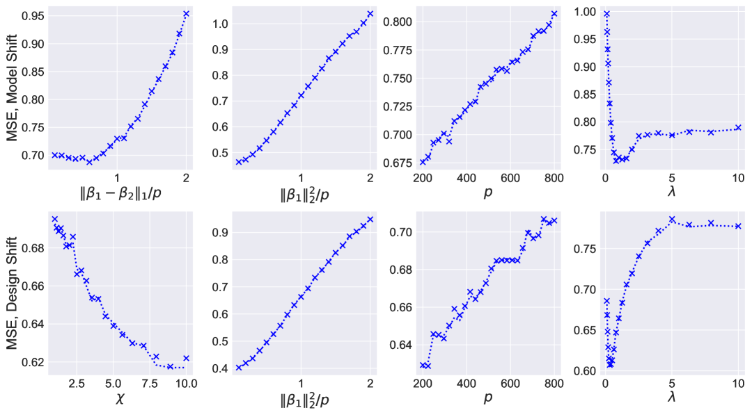
Figure 3: MSE for $\hat{\beta}_{\textup{II}}$. Same settings as in Figure 1 with $\lambda_{\textup{II}}=0.5$.

5 Extensions: Asymmetric and Multi-Environment GLAMP

In this section, we present Asymmetric GLAMP and Multi-Environment GLAMP, which are consequent formulations of the Symmetric GLAMP in Section 3. Asymmetric GLAMP is required for the introduction and proof of Multi-Environment GLAMP, which is in turn required for the proof of our transfer learning applications in Section 4.

5.1 Asymmetric GLAMP

Many previous AMP works—including the seminal paper by Donoho et al. [13]—adopt an alternative but equivalent formulation based on an asymmetric random matrix $X$, along with suitably defined auxiliary quantities. In this section, we articulate the asymmetric version of GLAMP following that tradition.

Definition 1 (Asymmetric GLAMP instance).

Let $q$ be a fixed and known positive integer, and consider the asymptotic regime where $\lim_{N\rightarrow+\infty}p/N\rightarrow\kappa\in(0,+\infty)$. An asymmetric GLAMP instance is defined as a tuple

$$\left\{X,(\Psi^{t})_{t\in\mathbb{N}},(\eta^{t})_{t\in\mathbb{N}},V^{0},B,W\right\},$$

with the following components:

• $X\in\mathbb{R}^{N\times p}$ is an asymmetric random design matrix;

• $B\in\mathbb{R}^{p\times q}$, $W\in\mathbb{R}^{N\times q}$ encode information accessible to the GLAMP iterates;

• $(\Psi^{t})_{t\in\mathbb{N}}$ and $(\eta^{t})_{t\in\mathbb{N}}$ are sequences of update mappings, where

  $$\Psi^{t}:\mathbb{R}^{N\times q}\times\mathbb{R}^{N\times q}\to\mathbb{R}^{N\times q},\quad\eta^{t}:\mathbb{R}^{p\times q}\times\mathbb{R}^{p\times q}\to\mathbb{R}^{p\times q};$$

• $V^{0}\in\mathbb{R}^{p\times q}$ is the initial condition for the GLAMP iterates.

As in prior formulations, the components $V^{0}$, $B$, and $W$ are omitted from notation when the context is clear. The following assumptions are associated with the asymmetric GLAMP instance:

Assumption 9 (Asymmetric GLAMP assumptions).

Given the GLAMP instance in Definition 1, we make the following assumptions:

1. The matrix $X\in\mathbb{R}^{N\times p}$ has i.i.d. entries drawn from $\mathcal{N}(0,1/N)$.

2. The matrices $B\in\mathbb{R}^{p\times q}$ and $W\in\mathbb{R}^{N\times q}$ satisfy

   $$\limsup_{p\to\infty}\frac{1}{\sqrt{p}}\|B\|_{2}<\infty,\quad\limsup_{N\to\infty}\frac{1}{\sqrt{N}}\|W\|_{2}<\infty.$$

3. The initial condition $V^{0}\in\mathbb{R}^{p\times q}$ satisfies

   $$\limsup_{p\to\infty}\frac{1}{p}\|V^{0}\|_{2}^{2}<\infty.$$

4. For each fixed $t\in\mathbb{N}$, the mappings $\Psi^{t}$ are uniformly Lipschitz in $N$, and $\eta^{t}$ are uniformly Lipschitz in $p$. In addition,

   $$\limsup_{N\to\infty}\frac{1}{\sqrt{N}}\|\Psi^{t}(0,0)\|_{2}<\infty,\quad\limsup_{p\to\infty}\frac{1}{\sqrt{p}}\|\eta^{t}(0,0)\|_{2}<\infty.$$

5. Fix $E\in\mathbb{N}_{+}$, and let $[N]=\bigcup_{a\in[E]}C_{a}^{N}$ be a sequence of partitions (groups) such that $\lim_{N\to\infty}|C_{a}^{N}|/N=c_{a}\in(0,1)$. For any $t\in\mathbb{N}$, the function $\Psi^{t}$ is separable across groups, i.e., there exist mappings

   $$\Psi_{a}^{t}:\mathbb{R}^{|C_{a}^{N}|\times q}\times\mathbb{R}^{|C_{a}^{N}|\times q}\to\mathbb{R}^{|C_{a}^{N}|\times q}$$

   such that

   $$\Psi^{t}(R^{t},W)=\begin{bmatrix}\Psi_{1}^{t}(R^{t}_{C_{1}^{N}},W_{C_{1}^{N}})\\ \Psi_{2}^{t}(R^{t}_{C_{2}^{N}},W_{C_{2}^{N}})\\ \vdots\\ \Psi_{E}^{t}(R^{t}_{C_{E}^{N}},W_{C_{E}^{N}})\end{bmatrix}.$$

6. The initial condition satisfies

   $$\frac{1}{p}\left(\eta^{0}(V^{0})\right)^{\top}\eta^{0}(V^{0})\to\Sigma_{(R)}^{0}$$

   for some matrix $\Sigma_{(R)}^{0}\in\mathbb{R}^{q\times q}$.

7. For any fixed covariance matrices $\Sigma_{1},\Sigma_{2}\in\mathbb{R}^{q\times q}$, and any $s,r\geq 0$, $a\in[E]$, the following limit exists:

   $$\lim_{N\to\infty}\frac{1}{|C_{a}^{N}|}\mathbb{E}\left[\Psi_{a}^{s}(Z_{1},W_{C_{a}^{N}})^{\top}\Psi_{a}^{r}(Z_{2},W_{C_{a}^{N}})\right],$$

   where $Z_{1},Z_{2}\in\mathbb{R}^{|C_{a}^{N}|\times q}$ have i.i.d. rows drawn from $\mathcal{N}(0,\Sigma_{1})$ and $\mathcal{N}(0,\Sigma_{2})$, respectively.

8. For any fixed covariance matrices $\Sigma_{1},\Sigma_{2}\in\mathbb{R}^{q\times q}$, and any $s,r\geq 1$, the following limits exist:

   $$\lim_{p\to\infty}\frac{1}{p}\mathbb{E}\left[\eta^{s}(Z_{1},B)^{\top}\eta^{r}(Z_{2},B)\right],\quad\lim_{p\to\infty}\frac{1}{p}\mathbb{E}\left[\eta^{0}(V^{0},B)^{\top}\eta^{r}(Z_{2},B)\right],$$

   where $Z_{1},Z_{2}\in\mathbb{R}^{p\times q}$ have i.i.d. rows drawn from $\mathcal{N}(0,\Sigma_{1})$ and $\mathcal{N}(0,\Sigma_{2})$, respectively.

Given an instance, the asymmetric GLAMP iterates and their corresponding state evolution are defined as follows:

Definition 2 (Asymmetric GLAMP iterates).

Let $\{X,(\Psi^{t})_{t\in\mathbb{N}},(\eta^{t})_{t\in\mathbb{N}},V^{0},B,W\}$ be an asymmetric GLAMP instance satisfying Assumption 9. The asymmetric GLAMP iterates are the alternating sequence of matrices $\{(V^{t},R^{t}):t\in\mathbb{N}\}$, initialized with

$$R^{0}=X\eta^{0}(V^{0},B).$$

For $t\in\mathbb{N_{+}}$, the iterates are defined recursively as:

$$V^{t} =\frac{1}{\kappa}X^{\top}\Psi^{t-1}(R^{t-1},W)-\frac{1}{\kappa}\eta^{t-1}(V^{t-1},B)\left[D_{(R)}^{t-1}\right]^{\top},\quad D_{(R)}^{t-1} =\frac{1}{N}\mathbb{E}\left[\sum_{j\in[N]}\left(\frac{\partial(\Psi^{t-1})_{j,\cdot}}{\partial(R^{t-1})_{j,\cdot}}\right)(Z_{(R)}^{t-1})\right],$$ (26)

$$R^{t} =X\eta^{t}(V^{t},B)-\Psi^{t-1}(R^{t-1},W)\left[D_{(V)}^{t}\right]^{\top},\quad D_{(V)}^{t} =\frac{1}{p}\mathbb{E}\left[\sum_{j\in[p]}\left(\frac{\partial(\eta^{t})_{j,\cdot}}{\partial(V^{t})_{j,\cdot}}\right)(Z_{(V)}^{t})\right],$$

where the Gaussian random matrices $Z_{(R)}^{t-1}$ and $Z_{(V)}^{t}$ will be defined in the state evolution equations (Definition 3).

Definition 3 (Asymmetric GLAMP state evolutions).

Starting from the initialization $\Sigma^{0}_{(R)}$ as given in Assumption 9 (f), we define a sequence of matrices as follows:

For $t\in\mathbb{N_{+}}$,

$$\Sigma^{t}_{(V)}=\lim_{N\to\infty}\frac{1}{N}\mathbb{E}\left[\Psi^{t-1}(Z^{t-1}_{(R)},W)^{\top}\Psi^{t-1}(Z^{t-1}_{(R)},W)\right],$$

where $Z^{t-1}_{(R)}\in\mathbb{R}^{N\times q}$ has i.i.d. rows drawn from $\mathcal{N}(0,\kappa\,\Sigma^{t-1}_{(R)})$.

Next,

$$\Sigma^{t}_{(R)}=\lim_{p\to\infty}\frac{1}{p}\mathbb{E}\left[\eta^{t}(Z^{t}_{(V)},B)^{\top}\eta^{t}(Z^{t}_{(V)},B)\right],$$

where $Z^{t}_{(V)}\in\mathbb{R}^{p\times q}$ has i.i.d. rows drawn from $\mathcal{N}(0,\frac{1}{\kappa^{2}}\Sigma^{t}_{(V)})$.

Corollary 1 (Asymmetric GLAMP convergence).

Let $t\in\mathbb{N}$. Consider the iterates defined in Definition 1 under Assumption 9. Then:

• For any order-$k$ pseudo-Lipschitz function $\phi:(\mathbb{R}^{p\times q})^{3}\to\mathbb{R}$, with $k\geq 1$, we have

  $$\phi(V^{t},V^{0},B)=\mathbb{E}\left[\phi(Z^{t}_{(V)},V^{0},B)\right]+o_{\mathsf{P}}(1),$$

  where $Z^{t}_{(V)}\in\mathbb{R}^{p\times q}$ has i.i.d. rows sampled from $\mathcal{N}(0,\kappa^{-2}\Sigma^{t}_{(V)})$, as defined in Definition 3.

• For any $a\in[E]$ and any order-$k$ pseudo-Lipschitz function $\phi:(\mathbb{R}^{|C_{a}^{N}|\times q})^{2}\to\mathbb{R}$, with $k\geq 1$, we have

  $$\phi(R^{t}_{C_{a}^{N}},W_{C_{a}^{N}})=\mathbb{E}\left[\phi(Z^{t}_{(R)},W_{C_{a}^{N}})\right]+o_{\mathsf{P}}(1),$$

  where $Z^{t}_{(R)}\in\mathbb{R}^{|C_{a}^{N}|\times q}$ has i.i.d. rows drawn from $\mathcal{N}(0,\kappa\Sigma^{t}_{(R)})$, also defined in Definition 3.

Corollary 1 is a direct consequence of Theorem 1, and its proof is omitted.

5.2 Multi-environment GLAMP

As a special case of the asymmetric GLAMP framework, we introduce the multi-environment GLAMP, which explicitly specifies each environment via the partition structure. In fact, all proofs related to the transfer learning applications presented in this work reduce to this specific formulation.

Definition 4 (Multi-environment GLAMP instance).

Suppose there are $E\in\mathbb{N}_{+}$ environments. Let $q$ be a fixed and known positive integer with $q=\sum_{e\in[E]}q_{e}$. Consider the asymptotic regime where

$$\lim_{p\to\infty}\frac{p}{n_{e}}\to\kappa_{e}\in(0,+\infty),\quad\forall\,e\in[E].$$

A multi-environment GLAMP instance is a tuple

$$\left(\bigcup_{e\in[E]}\left\{X_{e},(\Psi_{e}^{t})_{t\in\mathbb{N}},(\eta_{e}^{t})_{t\in\mathbb{N}},V_{e}^{0},W_{e}\right\}\right)\cup\{B\},$$

with the following components:

• For each $e\in[E]$, $X_{e}\in\mathbb{R}^{n_{e}\times p}$ is an asymmetric random design matrix;

• $B\in\mathbb{R}^{p\times q}$, and $W_{e}\in\mathbb{R}^{n_{e}\times q}$ encode information that the GLAMP iterates can use;

• $(\Psi_{e}^{t})_{t\in\mathbb{N}}$ is a sequence of mappings, with

  $$\Psi_{e}^{t}:\mathbb{R}^{n_{e}\times q_{e}}\times\mathbb{R}^{n_{e}\times q}\to\mathbb{R}^{n_{e}\times q_{e}};$$

• $(\eta_{e}^{t})_{t\in\mathbb{N}}$ is a sequence of mappings, with

  $$\eta_{e}^{t}:\left(\times_{e\in[E]}\mathbb{R}^{p\times q_{e}}\right)\times\mathbb{R}^{p\times q}\to\mathbb{R}^{p\times q_{e}};$$

• $V_{e}^{0}\in\mathbb{R}^{p\times q_{e}}$ is the initial condition of the asymmetric GLAMP iterates.

When the context is clear, the variables $V_{e}^{0}$, $W_{e}$, and $B$ may be omitted from the notation for simplicity.

Assumption 10 (Multi-environment GLAMP assumptions).

Consider the GLAMP instance in Definition 4. We impose the following assumptions:

1. For all $e\in[E]$, the matrix $X_{e}\in\mathbb{R}^{n_{e}\times p}$ has i.i.d. entries drawn from $\mathcal{N}(0,1/n_{e})$.

2. $\limsup_{p\to\infty}\frac{1}{\sqrt{p}}\|B\|_{2}<\infty$. For all $e\in[E]$, $\limsup_{n_{e}\to\infty}\frac{1}{\sqrt{n_{e}}}\|W_{e}\|_{2}<\infty$.

3. For all $e\in[E]$, the initialization $V_{e}^{0}\in\mathbb{R}^{p\times q_{e}}$ satisfies $\limsup_{p\to\infty}\frac{1}{p}\|V_{e}^{0}\|_{2}^{2}<\infty$.

4. For all $e\in[E]$ and all $t\in\mathbb{N}$, the mapping $\Psi_{e}^{t}$ is uniformly Lipschitz in $n_{e}$, and $\eta_{e}^{t}$ is uniformly Lipschitz in $p$. Moreover,

   $$\limsup_{n_{e}\to\infty}\frac{1}{\sqrt{n_{e}}}\|\Psi_{e}^{t}(0,0)\|_{2}<\infty,\quad\limsup_{p\to\infty}\frac{1}{\sqrt{p}}\|\eta_{e}^{t}(0,\dots,0)\|_{2}<\infty.$$

5. For all $e\in[E]$,

   $$\frac{1}{p}\left(\eta_{e}^{0}(V_{1}^{0},\dots,V_{E}^{0})\right)^{\top}\eta_{e}^{0}(V_{1}^{0},\dots,V_{E}^{0})\to\Sigma^{0}_{(R,e)}$$

   for some constant matrix $\Sigma^{0}_{(R,e)}\in\mathbb{R}^{q_{e}\times q_{e}}$.

6. For all $e\in[E]$, for any constant covariance matrices $\Sigma_{1},\Sigma_{2}\in\mathbb{R}^{q_{e}\times q_{e}}$, and for all $s,r\geq 0$,

   $$\lim_{n_{e}\to\infty}\frac{1}{n_{e}}\mathbb{E}\left[\Psi_{e}^{s}(Z_{1},W_{e})^{\top}\Psi_{e}^{r}(Z_{2},W_{e})\right]$$

   exists, where $Z_{1},Z_{2}\in\mathbb{R}^{n_{e}\times q_{e}}$ have i.i.d. rows drawn from $\mathcal{N}(0,\Sigma_{1})$ and $\mathcal{N}(0,\Sigma_{2})$, respectively.

7. For all $e\in[E]$, for any constant covariance matrices $\Sigma_{1},\Sigma_{2}\in\mathbb{R}^{q\times q}$, and for all $s,r\geq 1$,

   $$\lim_{p\to\infty}\frac{1}{p}\mathbb{E}\left[\eta_{e}^{s}(Z_{1},B)^{\top}\eta_{e}^{r}(Z_{2},B)\right],\quad\lim_{p\to\infty}\frac{1}{p}\mathbb{E}\left[\eta_{e}^{0}(V^{0},B)^{\top}\eta_{e}^{r}(Z_{2},B)\right]$$

   exist, where $Z_{1},Z_{2}\in\mathbb{R}^{p\times q}$ have i.i.d. rows drawn from $\mathcal{N}(0,\Sigma_{1})$ and $\mathcal{N}(0,\Sigma_{2})$, respectively.

Definition 5 (Multi-environment GLAMP iterates).

The multi-environment GLAMP iterates for an instance defined in Definition 4, under Assumption 10, are the alternating sequence of matrices

$$\left\{\left(V_{1}^{t},\dots,V_{E}^{t},R^{t}\right):t\in\mathbb{N}\right\},$$

initialized with $R_{e}^{0}=X_{e}\eta_{e}^{0}(V_{e}^{0},B)$ for each $e\in[E]$. For $t\in\mathbb{N_{+}}$, the updates are defined as follows:

$$V_{e}^{t}=\frac{1}{\kappa_{e}}X_{e}^{\top}\Psi_{e}^{t-1}(R_{e}^{t-1},W_{e})-\frac{1}{\kappa_{e}}\eta_{e}^{t-1}(V_{1}^{t-1},\dots,V_{E}^{t-1},B)\left[D_{(R,e)}^{t-1}\right]^{\top},$$ (27)

$$D_{(R,e)}^{t-1}=\frac{1}{n_{e}}\mathbb{E}\left[\sum_{j\in[n_{e}]}\left(\frac{\partial(\Psi_{e}^{t-1})_{j,\cdot}}{\partial(R_{e}^{t-1})_{j,\cdot}}\right)(Z_{(R,e)}^{t-1})\right],$$

$$R_{e}^{t}=X_{e}\eta_{e}^{t}(V_{1}^{t},\dots,V_{E}^{t},B)-\Psi_{e}^{t-1}(R_{e}^{t-1},W_{e})\left[D_{(V,e)}^{t}\right]^{\top},$$

$$D_{(V,e)}^{t}=\frac{1}{p}\mathbb{E}\left[\sum_{j\in[p]}\left(\frac{\partial(\eta_{e}^{t})_{j,\cdot}}{\partial(V_{e}^{t})_{j,\cdot}}\right)(Z_{(V,e)}^{t})\right],$$

where the Gaussian matrices $Z_{(R,e)}^{t-1}\in\mathbb{R}^{n_{e}\times q_{e}}$ and $Z_{(V,e)}^{t}\in\mathbb{R}^{p\times q}$ are defined in the state evolution (Definition 6).

Definition 6 (Multi-environment GLAMP state evolutions).

Starting from the initial covariance matrices $\{\Sigma^{0}_{(R,e)}:e\in[E]\}$ as specified in Assumption 9 (f), we define a sequence of matrices $\{\Sigma^{t}_{(V,e)},\Sigma^{t}_{(R,e)}:t\in\mathbb{N_{+}},\,e\in[E]\}$ as follows:

For each $e\in[E]$ and $t\in\mathbb{N_{+}}$,

$$\Sigma^{t}_{(V,e)}=\lim_{n_{e}\to\infty}\frac{1}{n_{e}}\mathbb{E}\left[\Psi_{e}^{t-1}(Z_{(R,e)}^{t-1},W_{e})^{\top}\Psi_{e}^{t-1}(Z_{(R,e)}^{t-1},W_{e})\right],$$

where $Z_{(R,e)}^{t-1}\in\mathbb{R}^{n_{e}\times q_{e}}$ has i.i.d. rows drawn from $\mathcal{N}(0,\kappa_{e}\Sigma^{t-1}_{(R,e)})$.

Next, define

$$\Sigma^{t}_{(R,e)}=\lim_{p\to\infty}\frac{1}{p}\mathbb{E}\left[\eta_{e}^{t}(Z_{(V,1)}^{t},\dots,Z_{(V,E)}^{t},B)^{\top}\eta_{e}^{t}(Z_{(V,1)}^{t},\dots,Z_{(V,E)}^{t},B)\right],$$

where for each $e\in[E]$, the matrix $Z^{t}_{(V,e)}\in\mathbb{R}^{p\times q_{e}}$ has i.i.d. rows drawn from

$$\mathcal{N}\left(0,\frac{1}{\kappa_{e}^{2}}\Sigma^{t}_{(V,e)}\right).$$

Corollary 2 (Multi-environment GLAMP convergence).

For the iterates defined in Definition 5 under Assumption 10, the following convergence results hold:

• For any $t\in\mathbb{N_{+}}$ and any order-$k$ pseudo-Lipschitz function $\phi:\left(\prod_{e\in[E]}\mathbb{R}^{p\times q_{e}}\right)^{2}\times\mathbb{R}^{p\times q}\to\mathbb{R}$, with $k\geq 1$, we have

  $$\phi(V_{1}^{t},\dots,V_{E}^{t},V_{1}^{0},\dots,V_{E}^{0},B)=\mathbb{E}\left[\phi(Z_{(V,1)}^{t},\dots,Z_{(V,E)}^{t},V_{1}^{0},\dots,V_{E}^{0},B)\right]+o_{\mathsf{P}}(1),$$

  where for each $e\in[E]$, the matrix $Z_{(V,e)}^{t}\in\mathbb{R}^{p\times q_{e}}$ has i.i.d. rows sampled from $\mathcal{N}\left(0,\frac{1}{\kappa_{e}^{2}}\Sigma_{(V,e)}^{t}\right),$ as defined in Definition 6, and the $Z_{(V,e)}^{t}$ are mutually independent across $e\in[E]$.

• For any $t\in\mathbb{N}$, $e\in[E]$, and any order-$k$ pseudo-Lipschitz function $\phi:(\mathbb{R}^{n_{e}\times q_{e}})^{2}\to\mathbb{R}$, with $k\geq 1$, we have

  $$\phi(R_{e}^{t},W_{e})=\mathbb{E}\left[\phi(Z_{(R,e)}^{t},W_{e})\right]+o_{\mathsf{P}}(1),$$

  where $Z_{(R,e)}^{t}\in\mathbb{R}^{n_{e}\times q_{e}}$ has i.i.d. rows drawn from $\mathcal{N}(0,\kappa_{e}\Sigma_{(R,e)}^{t}),$ as defined in Definition 6.

Corollary 2 is proved in Section A.5.

6 Discussion and Future Directions

In this paper, we introduce Generalized Long AMP (GLAMP), an extension of the AMP framework that accommodates both stacked iterations and non-separable denoising functions. Leveraging GLAMP, we derive precise asymptotic characterizations for three Lasso-based transfer learning estimators under proportional asymptotics. We conclude by outlining several promising directions for future research:

1. Extended Characterizations and Comparisons: Beyond the three Lasso-based estimators considered in this work, the GLAMP framework has the potential to analyze a broader class of estimators, including—but not limited to—those discussed in Section 2.2. Additionally, more comprehensive analytical and empirical comparisons could yield deeper insights into the performance of these methods across diverse transfer learning settings and offer more practical guidance for real-world applications.

2. Generalizing Assumptions: Our analysis assumes Gaussian design matrices; however, in many practical applications, covariates are often discrete or heavy-tailed. Extending existing universality results [65, 66, 67, 27, 68, 69, 70, 71, 72, 73] or AMP under right rotationally invariant designs [48, 50, 49, 70] to the GLAMP setting is an exciting avenue for future work.

3. Generalized Linear Models: Finally, we focused on linear models with continuous responses. However, GAMP has been successfully applied to logistic regression in prior work [17, 20] and extending our transfer learning applications of GLAMP to estimators in GLMs and classification problems [74, 75, 76, 77, 78] would be a natural avenue for future research.

Appendix A Proof of Theorem 1

A.1 Notations

Here we define additional notations that will be used in the proofs. For any matrix $M$, we denote the orthogonal projection onto its range $P_{M}$, and we let $P_{M}^{\bot}=I-P_{M}$. When $M$ has full column rank, we have $P_{M}=M(M^{\top}M)^{-1}M^{\top}$. We use $\{x^{0},f_{t}\}$ to denote a GLAMP instance $\{A,\{f_{t}\}_{t\in\mathbb{N}},x^{0},Y\}$ for simplicity, when the context is clear ($A,Y$ are fixed).

A.2 Proof of GLAMP Under the Non-Degeneracy Assumption

We first consider idealized Long AMP of the form:

$$h^{t+1}=P^{\bot}_{Q_{t-1}}AP^{\bot}_{Q_{t-1}}q^{t}+H_{t-1}\alpha^{t},\ \alpha^{t}=(Q_{t-1}^{{\top}}Q_{t-1})^{-1}Q_{t-1}^{{\top}}q^{t},$$ (A-1)

where $q^{0}=f_{0}(x^{0}),\ h^{1}=Aq^{0}$ as initialization; and for the matrices involved above, we define

$$Q_{t-1}= [q^{0}|q^{1}|\cdots|q^{t-1}]\in\mathbb{R}^{N\times(qt)},$$ (A-2)

$$\tilde{Q}_{t-1}= [q^{0}_{\bot}|q^{1}_{\bot}|\cdots|q^{t-1}_{\bot}]\in\mathbb{R}^{N\times(qt)},$$

$$Y_{t-1}= ~A\tilde{Q}_{t-1}=[Aq^{0}_{\bot}|Aq^{1}_{\bot}|\cdots|Aq^{t-1}_{\bot}]\in\mathbb{R}^{N\times(qt)},$$

$$H_{t-1}= ~[h^{1}|h^{2}|\cdots|h^{t}]\in\mathbb{R}^{N\times(qt)},$$

where $q^{t}=f_{t}(h^{t})$, $q^{t}_{\bot}=P_{Q_{t-1}}^{\bot}q^{t}$, $q^{t}_{\parallel}=P_{Q_{t-1}}q^{t}$ and $y^{t}=Aq^{t}_{\bot}$.

We define the sigma algebra $\mathfrak{S}_{t}=\sigma(h^{1},h^{2},\cdots,h^{t})$.

Assumption A.11 (Non-degeneracy).

The Long AMP iterates defined in Equation (A-1) meet the non-degeneracy assumption if we have both

1. Almost surely $\forall\,t\in\mathbb{N_{+}},N\geq qt$, $Q_{t-1}$ has full column rank.

2. Almost surely $\forall\,t\in\mathbb{N_{+}}$, $\liminf_{N\to\infty}\frac{1}{\sqrt{N}}\sigma_{\min}(Q_{t-1})\geq c_{t}>0$.

Lemma A.1.

Under Assumption A.11, we have $h^{t+1}|_{\mathfrak{S}_{t}}\stackrel{{\scriptstyle\mathrm{d}}}{{=}}P^{\bot}_{Q_{t-1}}\tilde{A}q^{t}_{\bot}+H_{t-1}\alpha^{t}$, where $\tilde{A}$ is an independent copy of $A$. Further, we have $h^{t+1}_{C_{a}^{N}}|_{\mathfrak{S}_{t}}\stackrel{{\scriptstyle\mathrm{d}}}{{=}}\tilde{A}_{C_{a}^{N},C_{a}^{N}}(q_{\bot}^{t})_{C_{a}^{N}}+\tilde{A}_{C_{a}^{N},(C_{a}^{N})^{c}}(q_{\bot}^{t})_{(C_{a}^{N})^{c}}-(\tilde{Q}_{t-1})_{C_{a}^{N}}(\tilde{Q}_{t-1}^{{\top}}\tilde{Q}_{t-1})^{-1}\tilde{Q}_{t-1}^{\top}\tilde{A}q^{t}_{\bot}+(H_{t-1})_{C_{a}^{N}}\alpha^{t}$.

The conditional distribution $h^{t+1}|_{\mathfrak{S}_{t}}$ can be analogously shown following the proof of Lemma 4, Berthier et al. [41]. In our case, $\tilde{Q}_{t-1}$ is no longer a strict Gram-Schmidt orthogonalized version of $Q_{t-1}$, but that does not change any step of the proof. The conditional distribution $h^{t+1}_{C_{a}^{N}}|_{\mathfrak{S}_{t}}$ follows with simple matrix algebra.

Lemma A.2.

Under Assumptions 1 and A.11, we have

1. $\forall\,0\leq s,r\leq t,$ and $a\in[E]$,

   $$\frac{1}{\lvert C_{a}^{N}\rvert}(h^{s+1}_{C_{a}^{N}})^{{\top}}h^{r+1}_{C_{a}^{N}}=\frac{1}{N}(q^{s})^{{\top}}q^{r}+o_{\mathsf{P}}(1),\ N\to\infty.$$ (A-3)

   In particular $\frac{1}{\lvert C_{a}^{N}\rvert}(h^{t+1}_{C_{a}^{N}})^{{\top}}h^{t+1}_{C_{a}^{N}}=\Sigma^{t+1}+o_{\mathsf{P}}(1)$.

2. $\forall\,t\in\mathbb{N}$ and any sequence of uniformly order-$k$ pseudo-Lipschitz functions $\{\phi_{N}:\mathbb{R}^{\lvert C_{a}^{N}\rvert\times[(t+3)q]}\to\mathbb{R}\}$ for any fixed $k\geq 1$,

   $$\phi_{N}([x^{0}_{C_{a}^{N}}|Y_{C_{a}^{N}}|h^{1}_{C_{a}^{N}}|\cdots|h^{t+1}_{C_{a}^{N}}])=\mathbb{E}_{Z}\left[\phi_{N}([x^{0}_{C_{a}^{N}}|Y_{C_{a}^{N}}|Z])\right]+o_{\mathsf{P}}(1),$$

   where $Z\in\mathbb{R}^{\lvert C_{a}^{N}\rvert\times[(t+1)q]}$, $Z^{{\top}}$ has iid column vectors drawn from $\mathcal{N}(0,\Sigma^{1:(t+1)})$ for some $\Sigma^{1:(t+1)}\in\mathbb{R}^{[(t+1)q]\times[(t+1)q]}$ that uniquely exists. $\Sigma^{1:t}=\frac{1}{N}Q_{t-1}^{{\top}}Q_{t-1}+o_{\mathsf{P}}(1)$; in particular, the total $(t+1)$ of $q$-by-$q$ diagonal blocks of $\Sigma^{1:(t+1)}$ are $\Sigma^{1},\Sigma^{2},\cdots,\Sigma^{t+1}$ from Definition 4.

The proof of Lemma A.2 is deferred to Section A.4.1.

Lemma A.3.

Under Assumptions 1 and A.11, for the GLAMP iterates in Equation 1 and LAMP iterates in Equation (A-1), $\forall\,t\in\mathbb{N}$,

$$\frac{1}{\sqrt{N}}\lVert h^{t+1}-x^{t+1}\rVert_{2}\stackrel{{\scriptstyle\mathbb{P}}}{{\to}}0,\quad\frac{1}{\sqrt{N}}\lVert q^{t}-m^{t}\rVert_{2}\stackrel{{\scriptstyle\mathbb{P}}}{{\to}}0.$$

The proof of Lemma A.3 is deferred to Section A.4.2.

Theorem A.1.

Under Assumption 1,A.11 and Definitions 1, 4, $\forall\,t\in\mathbb{N_{+}}$ and any sequence of uniformly order-$k$ pseudo-Lipschitz functions $\{\phi_{N}:\mathbb{R}^{\lvert C_{a}^{N}\rvert\times[(t+3)q]}\to\mathbb{R}\}$ for any fixed $k\geq 1$,

$$\phi_{N}([x^{0}_{C_{a}^{N}}|Y_{C_{a}^{N}}|x^{1}_{C_{a}^{N}}|\cdots|x^{t}_{C_{a}^{N}}])=\mathbb{E}_{Z}\left[\phi_{N}([x^{0}_{C_{a}^{N}}|Y_{C_{a}^{N}}|Z])\right]+o_{\mathsf{P}}(1),$$

where $Z\in\mathbb{R}^{\lvert C_{a}^{N}\rvert\times(tq)}$, $Z^{{\top}}$ has iid column vectors drawn from $\mathcal{N}(0,\Sigma^{1:t})$ for some $\Sigma^{1:t}\in\mathbb{R}^{(tq)\times(tq)}$ that uniquely exists. In particular, the total $t$ diagonal blocks of the size $q$-by-$q$ of $\Sigma^{1:t}$ are $\Sigma^{1},\Sigma^{2},\cdots,\Sigma^{t}$ from Definition 4.

Theorem A.1 is a direct corollary of Lemma A.2 and Lemma A.3, and we omit the proof here.

A.3 Proof of GLAMP in the General Case

Section A.2 has been working under Assumption A.11. In this section, we relax this assumption by adding a small Gaussian perturbation, so that any general GLAMP instance with perturbation satisfies Assumption A.11, and then making the perturbation vanish.

Throughout this section, we work on a general GLAMP instance satisfying Assumption 1, but not necessarily Assumption A.11. For each $t\in\mathbb{N}$, we add the following perturbation which effectively induces a new GLAMP instance:

$$f^{\epsilon y}_{t}(\cdot)=f_{t}(\cdot)+\epsilon y^{t},$$ (A-4)

where $\epsilon>0$ is a small constant, and $\{y^{t}:t\in\mathbb{N}\}$ is a sequence of iid random matrices in $\mathbb{R}^{N\times q}$, and $(y^{t})_{i,j}\stackrel{{\scriptstyle\mathrm{iid}}}{{\sim}}\mathcal{N}(0,1)$ for $(i,j)\in[N]\times[q]$. We use the subscript $\epsilon y$ on other quantities induced by this new GLAMP instance, and we omit the full notations for conciseness.

Lemma A.4 verifies that the newly constructed AMP instance satisfies all the necessary assumptions.

Counterpart of Lemma 8 and 9, Berthier et al. [41]

Lemma A.4.

Almostly surely w.r.t. $\{y^{t}:t\in\mathbb{N}\}$, if the original GLAMP setting $\{x^{0},f_{t}\}$ satisfies Assumption 1, then the GLAMP setting with $\{x^{0},f_{t}^{\epsilon y}\}$ satisfies Assumption  1 and A.11.

Let the state evolution of the original GLAMP setting $\{x^{0},f_{t}\}$ (which satisfies Assumption 1) be described by $\{(\hat{\Sigma}^{t}_{a},{\Sigma}^{t}):t\in\mathbb{N}\}$ according to Defintion 4. Then, the newly constructed instance $\{x^{0},f_{t}^{\epsilon y}\}$ satisfies Assumption 1(f) with matrices $\hat{\Sigma}^{\epsilon,0}_{a}=\hat{\Sigma}^{0}_{a}+\epsilon^{2}I_{q}$, and its state evolution from Definition 4 is almost surely

$${\Sigma}^{\epsilon,t}={\Sigma}^{t}+\epsilon^{2}I_{p},\quad\hat{\Sigma}^{\epsilon,t}_{a}=\hat{\Sigma}^{t}_{a}+\epsilon^{2}I_{p},$$

which does not depend on any special realization of $\{y^{t}:t\in\mathbb{N}\}$.

Lemma A.4 is proved in Section A.4.3.

Counterpart of Lemma 11, Berthier et al. [41]

Lemma A.5.

For the perturbed GLAMP setting $\{x^{0},f_{t}^{\epsilon y}\}$, if we denote its iterates as $x^{\epsilon y,t}$ for all $t\in\mathbb{N_{+}}$, then for any sequence of uniformly order-$k$ pseudo-Lipschitz functions $\{\phi_{N}:\mathbb{R}^{\lvert C_{a}^{N}\rvert\times[(t+3)q]}\to\mathbb{R}\}$ for any fixed $k\geq 1$,

$$\phi_{N}([x^{0}_{C_{a}^{N}}|Y_{C_{a}^{N}}|x^{\epsilon y,1}_{C_{a}^{N}}|\cdots|x^{\epsilon y,t}_{C_{a}^{N}}])=\mathbb{E}_{Z}\left[\phi_{N}([x^{0}_{C_{a}^{N}}|Y_{C_{a}^{N}}|Z])\right]+o_{\mathsf{P}}(1),$$

where $Z\in\mathbb{R}^{\lvert C_{a}^{N}\rvert\times(tq)}$, $Z^{{\top}}$ has iid column vectors drawn from $\mathcal{N}(0,\Sigma^{\epsilon,1:t})$ for some $\Sigma^{\epsilon,1:t}\in\mathbb{R}^{(tq)\times(tq)}$ that uniquely exists. The matrix $\Sigma^{\epsilon,1:t}$ satisfies:

1. The $t$ diagonal blocks of the size $q$-by-$q$ of $\Sigma^{\epsilon,1:t}$ are $\Sigma^{\epsilon,1},\Sigma^{\epsilon,2},\cdots,\Sigma^{\epsilon,t}$ defined in Lemma A.4.

2. $\lim_{\epsilon\downarrow 0}\Sigma^{\epsilon,1:t}=\Sigma^{1:t}$ for some positive semi-definite matrix $\Sigma^{1:t}$. The $t$ diagonal blocks of the size $q$-by-$q$ of $\Sigma^{1:t}$ are $\Sigma^{1},\Sigma^{2},\cdots,\Sigma^{t}$ from the state evolution of the unperturbed setting $\{x^{0},f_{t}\}$.

Lemma A.5 is proved in Section A.4.4.

Counterpart of Lemma 12, Berthier et al. [41]

Lemma A.6.

For any GLAMP setting $\{x^{0},f_{t}\}$ satifying Assumption 1 and its perturbed settings $\{x^{0},f^{\epsilon y}_{t}\}$ for $\epsilon\in(0,1]$, for any fixed $t\in\mathbb{N_{+}}$, there exists some functions $h_{t}(\epsilon)$ defined for $\epsilon\in[0,1]$ and free of $N$, s.t. $\lim_{\epsilon\downarrow 0}h_{t}(\epsilon)=0$, and (treating $x^{\epsilon y,0}=x^{0}$)

$$\lim_{N\to\infty}\mathbb{P}\left[\frac{1}{\sqrt{N}}\lVert f^{\epsilon y}_{t-1}(x^{\epsilon y,t-1})-f_{t-1}(x^{t-1})\rVert_{2}\leq h_{t}(\epsilon)\right]=1,\quad\lim_{N\to\infty}\mathbb{P}\left[\frac{1}{\sqrt{N}}\lVert x^{\epsilon y,t}-x^{t}\rVert_{2}\leq h_{t}(\epsilon)\right]=1.$$

Lemma A.6 is proved in Section A.4.5. As a special note on Lemma A.6, we don’t additionally assume anything like ‘$\Sigma^{1},\Sigma^{2},\cdots,\Sigma^{t}$ are all strictly positive definite for some $t\in\mathbb{N_{+}}$’ like the counterpart in Berthier et al. [41] (Lemma 12) does. We drop this condition and provide a more general proof, because such an assumption could be unrealistic. For example, the GAMP formulation for logistic regression in Sur and Candès [17], $f_{t}$ has a lot of constant functions along the $q$ axis.

Theorem A.2.

Under Assumption 1 and Definitions 1, 4, $\forall\,t\in\mathbb{N_{+}}$ and any sequence of uniformly order-$k$ pseudo-Lipschitz functions $\{\phi_{N}:\mathbb{R}^{\lvert C_{a}^{N}\rvert\times[(t+3)q]}\to\mathbb{R}\}$ for any fixed $k\geq 1$,

$$\phi_{N}([x^{0}_{C_{a}^{N}}|Y_{C_{a}^{N}}|x^{1}_{C_{a}^{N}}|\cdots|x^{t}_{C_{a}^{N}}])=\mathbb{E}_{Z}\left[\phi_{N}([x^{0}_{C_{a}^{N}}|Y_{C_{a}^{N}}|Z])\right]+o_{\mathsf{P}}(1),$$

where $Z\in\mathbb{R}^{\lvert C_{a}^{N}\rvert\times(tq)}$, $Z^{{\top}}$ has iid column vectors drawn from $\mathcal{N}(0,\Sigma^{1:t})$ for some $\Sigma^{1:t}\in\mathbb{R}^{(tq)\times(tq)}$ that uniquely exists. In particular, the total $t$ diagonal blocks of the size $q$-by-$q$ of $\Sigma^{1:t}$ are $\Sigma^{1},\Sigma^{2},\cdots,\Sigma^{t}$ from Definition 4.

Proof of Theorem A.2.

For any sequence of uniformly order-$k$ pseudo-Lipschitz functions $\{\phi_{N}:\mathbb{R}^{\lvert C_{a}^{N}\rvert\times[(t+3)q]}\to\mathbb{R}\}$ with fixed $k\geq 1$, for any $\eta>0$, there exists some $\epsilon>0$, such that under the perturbed setting $\{x^{0},f^{\epsilon y}_{t}\}$, when $N$ is large enough, we have

$$~\mathbb{P}\left[\left\lvert\phi_{N}([x^{0}_{C_{a}^{N}}|Y_{C_{a}^{N}}|x^{1}_{C_{a}^{N}}|\cdots|x^{t}_{C_{a}^{N}}])-\mathbb{E}_{Z}\left[\phi_{N}([x^{0}_{C_{a}^{N}}|Y_{C_{a}^{N}}|Z])\right]\right\rvert\geq 3\eta\right]$$ (A-5)

$$\leq ~\mathbb{P}\left[\left\lvert\phi_{N}([x^{0}_{C_{a}^{N}}|Y_{C_{a}^{N}}|x^{\epsilon y,1}_{C_{a}^{N}}|\cdots|x^{\epsilon y,t}_{C_{a}^{N}}])-\mathbb{E}_{Z}\left[\phi_{N}([x^{0}_{C_{a}^{N}}|Y_{C_{a}^{N}}|Z^{\epsilon}])\right]\right\rvert\geq\eta\right]$$

$$~+\mathbb{P}\left[\left\lvert\phi_{N}([x^{0}_{C_{a}^{N}}|Y_{C_{a}^{N}}|x^{\epsilon y,1}_{C_{a}^{N}}|\cdots|x^{\epsilon y,t}_{C_{a}^{N}}])-\phi_{N}([x^{0}_{C_{a}^{N}}|Y_{C_{a}^{N}}|x^{1}_{C_{a}^{N}}|\cdots|x^{t}_{C_{a}^{N}}])\right\rvert\geq\eta\right]$$

$$~+\mathbf{1}{\{\left\lvert\mathbb{E}_{Z}\left[\phi_{N}([x^{0}_{C_{a}^{N}}|Y_{C_{a}^{N}}|Z^{\epsilon}])\right]-\mathbb{E}_{Z}\left[\phi_{N}([x^{0}_{C_{a}^{N}}|Y_{C_{a}^{N}}|Z])\right]\right\rvert>\eta\}},$$

where $Z^{\epsilon},Z\in\mathbb{R}^{N\times q}$, $Z^{\epsilon}$ has iid rows from $\mathcal{N}(0,\Sigma^{\epsilon,1:t})$ and $Z$ has iid rows from $\mathcal{N}(0,\Sigma^{1:t})$ introduced in Lemma A.5.

By Lemma F.5, since $\lim_{\epsilon\downarrow 0}\Sigma^{\epsilon,1:t}=\Sigma^{1:t}$ by Lemma A.5, we can fix $\epsilon$ small enough s.t. the third term on the RHS of Equation (A-5) is zero.

Since the perturbed setting $\{x^{0},f^{\epsilon y}_{t}\}$ satisfies Assumption  1 by Lemma A.4, we can apply Theorem A.1 with any fixed $\epsilon$ and get that the first term on the RHS of Equation (A-5) goes to zero as $N\to+\infty$.

We finally look at the second term on the RHS of Equation (A-5). Since $\lvert C_{a}^{N}\rvert/N\to c_{a}>0$, we use $N$ in the denominators just to save notation:

$$~\left\lvert\phi_{N}([x^{0}_{C_{a}^{N}}|Y_{C_{a}^{N}}|x^{\epsilon y,1}_{C_{a}^{N}}|\cdots|x^{\epsilon y,t}_{C_{a}^{N}}])-\phi_{N}([x^{0}_{C_{a}^{N}}|Y_{C_{a}^{N}}|x^{1}_{C_{a}^{N}}|\cdots|x^{t}_{C_{a}^{N}}])\right\rvert$$

$$\leq ~L\left[1+\left(\frac{\lVert x^{0}_{C_{a}^{N}}\rVert_{2}}{\sqrt{N}}\right)^{k-1}+\left(\frac{\lVert Y_{C_{a}^{N}}\rVert_{2}}{\sqrt{N}}\right)^{k-1}+\sum_{t_{0}\in[t]}\left(\frac{\lVert x^{t_{0}}_{C_{a}^{N}}\rVert_{2}}{\sqrt{N}}\right)^{k-1}+\sum_{t_{0}\in[t]}\left(\frac{\lVert x^{\epsilon y,t_{0}}_{C_{a}^{N}}\rVert_{2}}{\sqrt{N}}\right)^{k-1}\right]$$

$$\cdot \frac{\sum_{t_{0}\in[t]}\lVert x^{\epsilon y,t_{0}}_{C_{a}^{N}}-x^{t_{0}}_{C_{a}^{N}}\rVert_{2}}{\sqrt{N}}.$$

Inside the first square brackets, all the terms have tractable upper bounds with high probability as $N\to+\infty$. For $x^{0}_{C_{a}^{N}}$ and $Y_{C_{a}^{N}}$, this is guaranteed by Assumption 1(f). For the other terms, they are guaranteed by the later Lemma A.8. For the last component, we know from Lemma A.6 that

$$\lim_{N\to+\infty}\mathbb{P}\left[\frac{1}{\sqrt{N}}\sum_{t_{0}\in[t]}\lVert x^{\epsilon y,t_{0}}_{C_{a}^{N}}-x^{t_{0}}_{C_{a}^{N}}\rVert_{2}\leq\sum_{t_{0}\in[t]}h_{t_{0}}(\epsilon)\right]=1.$$

Since $\lim_{\epsilon\downarrow 0}\sum_{t_{0}\in[t]}h_{t_{0}}(\epsilon)=0$, we can fix $\epsilon$ small enough, s.t.

$$\lim_{N\rightarrow+\infty}\mathbb{P}\left[\left\lvert\phi_{N}([x^{0}_{C_{a}^{N}}|Y_{C_{a}^{N}}|x^{\epsilon y,1}_{C_{a}^{N}}|\cdots|x^{\epsilon y,t}_{C_{a}^{N}}])-\phi_{N}([x^{0}_{C_{a}^{N}}|Y_{C_{a}^{N}}|x^{1}_{C_{a}^{N}}|\cdots|x^{t}_{C_{a}^{N}}])\right\rvert\leq\eta\right]=1.$$

Now that we have addressed all the three terms on the RHS of Equation (A-5), we have thus proved

$$\phi_{N}([x^{0}_{C_{a}^{N}}|Y_{C_{a}^{N}}|x^{t}_{C_{a}^{N}}])=\mathbb{E}\left[\phi_{N}(x^{0}_{C_{a}^{N}}|Y_{C_{a}^{N}}|Z^{t}_{a})\right]+o_{\mathsf{P}}(1).$$

∎

A.4 Proof of Auxiliary Lemmas in Sections A.2 and A.3

A.4.1 Proof of Lemma A.2

We will be using induction. As a shorthand, denote $\mathcal{H}_{t}$ as the statement of both Lemma A.2 (a) and (b) being true for a certain $t$, $t\in\mathbb{N}$. We start from $t=0$.

Proof of $\mathcal{H}_{0}$: Now $h^{1}=Aq^{0}$, which means $h^{1}_{C_{a}^{N}}=A_{C_{a}^{N},\cdot}q^{0}=A_{C_{a}^{N},C_{a}^{N}}q^{0}_{C_{a}^{N}}+A_{C_{a}^{N},(C_{a}^{N})^{c}}q^{0}_{(C_{a}^{N})^{c}}$.

For the first term, we can prove $\frac{1}{\lvert C_{a}^{N}\rvert}(A_{C_{a}^{N},C_{a}^{N}}q^{0}_{C_{a}^{N}})^{{\top}}A_{C_{a}^{N},C_{a}^{N}}q^{0}_{C_{a}^{N}}=c_{a}\hat{\Sigma}_{a}^{0}+o_{\mathsf{P}}(1)$ with Lemma F.2(d). For the second term, $A_{C_{a}^{N},(C_{a}^{N})^{c}}$ is just an iid Gaussian matrix, so the limit is easy to study. By the LLN, we can prove that $\frac{1}{N}(A_{C_{a}^{N},C_{a}^{N}}q^{0}_{C_{a}^{N}})^{{\top}}A_{C_{a}^{N},(C_{a}^{N})^{c}}q^{0}_{(C_{a}^{N})^{c}}\to 0$ and $\frac{1}{\lvert C_{a}^{N}\rvert}(A_{C_{a}^{N},(C_{a}^{N})^{c}}q^{0}_{(C_{a}^{N})^{c}})^{{\top}}A_{C_{a}^{N},(C_{a}^{N})^{c}}q^{0}_{(C_{a}^{N})^{c}}\to\sum_{a^{\prime}\neq a}c_{a^{\prime}}\hat{\Sigma}^{0}_{a^{\prime}}$, both almost surely. To sum up, we have verified

$$\frac{1}{\lvert C_{a}^{N}\rvert}(h^{1}_{C_{a}^{N}})^{{\top}}h^{1}_{C_{a}^{N}}=\frac{1}{N}(q^{0})^{{\top}}q^{0}+o_{\mathsf{P}}(1)=\sum_{a\in[E]}c_{a}\hat{\Sigma}^{0}_{a}+o_{\mathsf{P}}(1).$$

Based on the above, Part (b) can be verified with Lemma F.2(d) given Assumption 1 about the boundedness of $x^{0}$ and $Y$.

Proof of $\mathcal{H}_{t}$ given $\mathcal{H}_{0},\mathcal{H}_{1},\cdots,\mathcal{H}_{t-1}$: Wtih the induction hypothesis and Lemma A.1, we first point out

$$\frac{1}{\sqrt{\lvert C_{a}^{N}\rvert}}h^{t+1}_{C_{a}^{N}}|_{\mathfrak{S}_{t}}\stackrel{{\scriptstyle\mathrm{d}}}{{=}}\frac{1}{\sqrt{\lvert C_{a}^{N}\rvert}}\tilde{A}_{C_{a}^{N},C_{a}^{N}}(q_{\bot}^{t})_{C_{a}^{N}}+\frac{1}{\sqrt{\lvert C_{a}^{N}\rvert}}\tilde{A}_{C_{a}^{N},(C_{a}^{N})^{c}}(q_{\bot}^{t})_{(C_{a}^{N})^{c}}+\frac{1}{\sqrt{\lvert C_{a}^{N}\rvert}}(H_{t-1})_{C_{a}^{N}}\alpha^{t}+o_{\mathsf{P}}(1).$$ (A-6)

To show Equation (A-6), we only need $\frac{1}{\sqrt{\lvert C_{a}^{N}\rvert}}(\tilde{Q}_{t-1})_{C_{a}^{N}}(\tilde{Q}_{t-1}^{{\top}}\tilde{Q}_{t-1})^{-1}\tilde{Q}_{t-1}^{\top}\tilde{A}q^{t}_{\bot}=o_{\mathsf{P}}(1)$. This is because $P_{Q_{t-1}}\tilde{A}q_{\bot}^{t}/\sqrt{N}=o_{\mathsf{P}}(1)$ by Lemma F.2(b) and the induction hypothesis.

We first consider $\mathcal{H}_{t}(a)$ for $s<r=t$. Since $\frac{1}{\lvert C_{a}^{N}\rvert}(h_{C_{a}^{N}}^{s+1})^{{\top}}h_{C_{a}^{N}}^{s+1}=\Sigma^{s+1}+o_{\mathsf{P}}(1)$, $\frac{1}{\sqrt{\lvert C_{a}^{N}\rvert}}h_{C_{a}^{N}}^{s+1}$ must be of a bounded norm. Then we have

$$\left(\frac{1}{\lvert C_{a}^{N}\rvert}(h_{C_{a}^{N}}^{s+1})^{{\top}}h_{C_{a}^{N}}^{t+1}-\frac{1}{N}(q^{s})^{\top}q^{t}\middle)\right|_{\mathfrak{S}_{t}}\stackrel{{\scriptstyle\mathrm{d}}}{{=}} ~\frac{1}{\lvert C_{a}^{N}\rvert}(h_{C_{a}^{N}}^{s+1})^{{\top}}\tilde{A}_{C_{a}^{N},C_{a}^{N}}(q_{\bot}^{t})_{C_{a}^{N}}$$

$$~+\frac{1}{\lvert C_{a}^{N}\rvert}(h_{C_{a}^{N}}^{s+1})^{{\top}}\tilde{A}_{C_{a}^{N},(C_{a}^{N})^{c}}(q_{\bot}^{t})_{(C_{a}^{N})^{c}}$$

$$~+\frac{1}{\lvert C_{a}^{N}\rvert}(h_{C_{a}^{N}}^{s+1})^{{\top}}(H_{t-1})_{C_{a}^{N}}\alpha^{t}-\frac{1}{N}(q^{s})^{\top}q^{t}+o_{\mathsf{P}}(1).$$

The first term goes to zero in probability by Lemma F.2(a). The second term also goes to zero in probability because it is a normal variable whose variance is at the scale of $1/N$. For the last two terms, we have $\frac{1}{\lvert C_{a}^{N}\rvert}(h_{C_{a}^{N}}^{s+1})^{{\top}}(H_{t-1})_{C_{a}^{N}}\alpha^{t}-\frac{1}{N}(q^{s})^{\top}q^{t}=o_{\mathsf{P}}(1)$ analogously to Equation (95)-(97) of Berthier et al. [41]. In particular, we know $\alpha^{t}=\alpha^{t,*}+o_{\mathsf{P}}(1)$, the latter being a nonrandom matrix in $\mathbb{R}^{(tq)\times q}$, whose definition we omit for conciseness.

We then consider $\mathcal{H}_{t}$(a) for $s=r=t$. As $\frac{1}{\lvert C_{a}^{N}\rvert}(h_{C_{a}^{N}}^{t+1})^{{\top}}h_{C_{a}^{N}}^{t+1}|_{\mathfrak{S}_{t}}$ is going to be lengthy, we first simplify it with Equation (A-6). Moreover, for the three major terms on the RHS of Equation (A-6), their cross terms are all zero. Conditioning on $\mathfrak{S}_{t}$, the second term is independent of the other two, so any cross term involving it is eventually a Gaussian whose variance is at the scale of $1/N$, thus $o_{\mathsf{P}}(1)$. For the cross terms involving the first and third terms, we can use Lemma F.2(a) to conclude they are zero. As a result,

$$\left(\frac{1}{\lvert C_{a}^{N}\rvert}(h_{C_{a}^{N}}^{t+1})^{{\top}}h_{C_{a}^{N}}^{t+1}-\frac{1}{N}(q^{t})^{\top}q^{t}\middle)\right|_{\mathfrak{S}_{t}}\stackrel{{\scriptstyle\mathrm{d}}}{{=}} ~\frac{1}{\lvert C_{a}^{N}\rvert}(\tilde{A}_{C_{a}^{N},C_{a}^{N}}(q_{\bot}^{t})_{C_{a}^{N}})^{{\top}}\tilde{A}_{C_{a}^{N},C_{a}^{N}}(q_{\bot}^{t})_{C_{a}^{N}}$$ (A-7)

$$~+\frac{1}{\lvert C_{a}^{N}\rvert}(q_{\bot}^{t})_{(C_{a}^{N})^{c}}^{{\top}}(\tilde{A}_{C_{a}^{N},(C_{a}^{N})^{c}})^{{\top}}\tilde{A}_{C_{a}^{N},(C_{a}^{N})^{c}}(q_{\bot}^{t})_{(C_{a}^{N})^{c}}$$

$$~+\frac{1}{\lvert C_{a}^{N}\rvert}(\alpha^{t})^{{\top}}(H_{t-1})_{C_{a}^{N}}^{{\top}}(H_{t-1})_{C_{a}^{N}}\alpha^{t}-\frac{1}{N}(q^{t})^{\top}q^{t}+o_{\mathsf{P}}(1).$$

To study the first term on the RHS of Equation (A-7), we want to ultimately invoke Lemma F.2(d), but for that we need to establish the probability limit of $\frac{1}{N}(q^{t}_{\bot})^{{\top}}_{C_{a}^{N}}(q^{t}_{\bot})_{C_{a}^{N}}$, which we will go out of our way to do first. We know $q^{s}_{C_{a}^{N}}=g_{s,a}(h^{s}_{C_{a}^{N}},Y_{C_{a}^{N}})$ for any time step $s$. By $\mathcal{H}_{t-1}$(b) and Assumption 1(g), $\frac{1}{N}(q^{t}_{C_{a}^{N}})^{{\top}}q^{t}_{C_{a}^{N}}=c_{a}\hat{\Sigma}^{t}_{a}$, and $\frac{1}{N}(q^{t}_{C_{a}^{N}})^{{\top}}(Q_{t-1})_{C_{a}^{N}}$ also has a well-defined limit in probability. Since we can write $(q^{t}_{\parallel})_{C_{a}^{N}}=(Q_{t-1})_{C_{a}^{N}}\alpha^{t}$, we know each of $\frac{1}{N}(q^{t}_{C_{a}^{N}})^{{\top}}(q^{t}_{C_{a}^{N}})$, $\frac{1}{N}(q^{t}_{\parallel})_{C_{a}^{N}}^{{\top}}(q^{t}_{\parallel})_{C_{a}^{N}}$, $\frac{1}{N}(q^{t}_{C_{a}^{N}})^{{\top}}(q^{t}_{\parallel})_{C_{a}^{N}}$ has a limit in probability. Thus so does $\frac{1}{N}(q^{t}_{\bot})^{{\top}}_{C_{a}^{N}}(q^{t}_{\bot})_{C_{a}^{N}}$. Invoking Lemma F.2(d), we finally have

$$\frac{1}{\lvert C_{a}^{N}\rvert}(\tilde{A}_{C_{a}^{N},C_{a}^{N}}(q_{\bot}^{t})_{C_{a}^{N}})^{{\top}}\tilde{A}_{C_{a}^{N},C_{a}^{N}}(q_{\bot}^{t})_{C_{a}^{N}}=\frac{1}{N}(q^{t}_{\bot})_{C_{a}^{N}}^{{\top}}(q^{t}_{\bot})_{C_{a}^{N}}+o_{\mathsf{P}}(1).$$ (A-8)

To study the second term on the RHS of Equation (A-7), we can just use the LLN to get

$$\frac{1}{\lvert C_{a}^{N}\rvert}(q_{\bot}^{t})_{(C_{a}^{N})^{c}}^{{\top}}(\tilde{A}_{C_{a}^{N},(C_{a}^{N})^{c}})^{{\top}}\tilde{A}_{C_{a}^{N},(C_{a}^{N})^{c}}(q_{\bot}^{t})_{(C_{a}^{N})^{c}}=\frac{1}{N}(q_{\bot}^{t})_{(C_{a}^{N})^{c}}^{{\top}}(q_{\bot}^{t})_{(C_{a}^{N})^{c}}+o_{\mathsf{P}}(1).$$ (A-9)

To study the third term on the RHS of Equation (A-7), we use $\mathcal{H}_{t-1}(a)$ to change $\frac{1}{\lvert C_{a}^{N}\rvert}(H_{t-1})_{C_{a}^{N}}^{{\top}}(H_{t-1})_{C_{a}^{N}}$ to $\frac{1}{N}Q_{t-1}^{{\top}}Q_{t-1}$. Eventually we have

$$\frac{1}{\lvert C_{a}^{N}\rvert}(\alpha^{t})^{{\top}}(H_{t-1})_{C_{a}^{N}}^{{\top}}(H_{t-1})_{C_{a}^{N}}\alpha^{t}=\frac{1}{N}(q^{t}_{\parallel})^{\top}q^{t}_{\parallel}+o_{\mathsf{P}}(1).$$ (A-10)

Combining the above, we have proved $\frac{1}{\lvert C_{a}^{N}\rvert}(h_{C_{a}^{N}}^{t+1})^{{\top}}h_{C_{a}^{N}}^{t+1}=\frac{1}{N}(q^{t})^{\top}q^{t}+o_{\mathsf{P}}(1)$. To complete $\mathcal{H}_{t}$(a), we are left to verify $\frac{1}{N}(q^{t})^{\top}q^{t}=\Sigma^{t+1}+o_{\mathsf{P}}(1)$. Using $\mathcal{H}_{t-1}$(b), we have

$$\frac{1}{N}(q^{t})^{\top}q^{t}= ~\sum_{a\in[E]}\frac{\lvert C_{a}^{N}\rvert}{N}\cdot\frac{1}{\lvert C_{a}^{N}\rvert}g_{t,a}(h^{t}_{C_{a}^{N}},Y_{C_{a}^{N}})^{{\top}}g_{t,a}(h^{t}_{C_{a}^{N}},Y_{C_{a}^{N}})$$ (A-11)

$$= ~\sum_{a\in[E]}c_{a}\cdot\frac{1}{\lvert C_{a}^{N}\rvert}\mathbb{E}\left[g_{t,a}(Z^{t}_{a},Y_{C_{a}^{N}})^{{\top}}g_{t,a}(Z^{t}_{a},Y_{C_{a}^{N}})\right]+o_{\mathsf{P}}(1)$$

$$= ~\sum_{a\in[E]}c_{a}\hat{\Sigma}_{a}^{t}+o_{\mathsf{P}}(1)=\Sigma^{t+1}+o_{\mathsf{P}}(1).$$

This completes the proof of $\mathcal{H}_{t}$(a).

We next consider $\mathcal{H}_{t}(b)$. With all the intermediate result we have got, the rest of the proof is straightforward following $\mathcal{H}_{t}(b)$ of Lemma 5, Berthier et al. [41]. We first abbreviate $\phi^{\prime}_{N}(\cdot)=\phi_{N}([x^{0}_{C_{a}^{N}}|Y_{C_{a}^{N}}|h^{1}_{C_{a}^{N}}|\cdots|\cdot])$. Conditionally,

$$\phi^{\prime}_{N}(h^{t+1}_{C_{a}^{N}})|_{\mathfrak{S}_{t}}\stackrel{{\scriptstyle\mathrm{d}}}{{=}}\phi^{\prime}_{N}\left(\tilde{A}_{C_{a}^{N},C_{a}^{N}}(q_{\bot}^{t})_{C_{a}^{N}}+\tilde{A}_{C_{a}^{N},(C_{a}^{N})^{c}}(q_{\bot}^{t})_{(C_{a}^{N})^{c}}+(H_{t-1})_{C_{a}^{N}}\alpha^{t,*}\right)+o_{\mathsf{P}}(1),$$

where we have used Equation (A-6) to drop one term from $h^{t+1}|_{\mathfrak{S}_{t}}$ in Lemma A.1, used the fact that $\alpha^{t}=\alpha^{t,*}+o_{\mathsf{P}}(1),\,\alpha^{t,*}\in\mathbb{R}^{(tq)\times q}$ to replace $\alpha^{t}$ with $\alpha^{t,*}$, and used Equation (A-8), (A-9), (A-10) to guarantee the stochastic boundedness of the other terms.

On the RHS of the above equation, $\tilde{A}_{C_{a}^{N},C_{a}^{N}}\mathchoice{\mathrel{\hbox to0.0pt{$\displaystyle\perp$\hss}\mkern 2.0mu{\displaystyle\perp}}}{\mathrel{\hbox to0.0pt{$\textstyle\perp$\hss}\mkern 2.0mu{\textstyle\perp}}}{\mathrel{\hbox to0.0pt{$\scriptstyle\perp$\hss}\mkern 2.0mu{\scriptstyle\perp}}}{\mathrel{\hbox to0.0pt{$\scriptscriptstyle\perp$\hss}\mkern 2.0mu{\scriptscriptstyle\perp}}}\tilde{A}_{C_{a}^{N},(C_{a}^{N})^{c}}$. We can first apply Lemma F.2(d) and then Lemma F.3 to get

$$\phi^{\prime}_{N}(h^{t+1}_{C_{a}^{N}})|_{\mathfrak{S}_{t}}\stackrel{{\scriptstyle\mathrm{d}}}{{=}}\mathbb{E}_{Z}[\phi^{\prime}_{N}\left(Z+(H_{t-1})_{C_{a}^{N}}\alpha^{t,*}\right)]+o_{\mathsf{P}}(1),$$

where $Z\in\mathbb{R}^{\lvert C_{a}^{N}\rvert\times q}$, $Z^{{\top}}$ has column vectors drawn iid from $\mathcal{N}(0,\mathrm{plim}_{N}\frac{1}{N}(q^{t}_{\bot})^{{\top}}q^{t}_{\bot})$. (One technicality in applying Lemma F.3 is that each row of $\tilde{A}_{C_{a}^{N},(C_{a}^{N})^{c}}(q_{\bot}^{t})_{(C_{a}^{N})^{c}}$ is iid with a covariance matrix changing in $N$. To address this issue, we can lift $(\frac{1}{N}(q_{\bot}^{t})_{(C_{a}^{N})^{c}}^{{\top}}(q_{\bot}^{t})_{(C_{a}^{N})^{c}})^{1/2}$ out of the variance to allow for Lemma F.3, and then use Lemma F.5. To warrant the use of Lemma F.3, notice that $\frac{1}{N}(q_{\bot}^{t})_{(C_{a}^{N})^{c}}^{{\top}}(q_{\bot}^{t})_{(C_{a}^{N})^{c}}=\sum_{a^{\prime}\neq a}\frac{1}{N}(q_{\bot}^{t})_{(C_{a^{\prime}}^{N})^{c}}^{{\top}}(q_{\bot}^{t})_{(C_{a^{\prime}}^{N})^{c}}$; for each $a^{\prime}$, we have established that $\frac{1}{N}(q_{\bot}^{t})_{(C_{a^{\prime}}^{N})^{c}}^{{\top}}(q_{\bot}^{t})_{(C_{a^{\prime}}^{N})^{c}}$ has a tractable well-defined limit in probability, and thus $\frac{1}{N}(q_{\bot}^{t})_{(C_{a}^{N})^{c}}^{{\top}}(q_{\bot}^{t})_{(C_{a}^{N})^{c}}$ has a probability limit as well.)

Finally we apply the induction hypothesis to remove the condition,

$$\phi_{N}([x^{0}_{C_{a}^{N}}|Y_{C_{a}^{N}}|h^{1}_{C_{a}^{N}}|\cdots|h^{t+1}_{C_{a}^{N}}])=\mathbb{E}_{Z_{1}\mathchoice{\mathrel{\hbox to0.0pt{$\displaystyle\perp$\hss}\mkern 2.0mu{\displaystyle\perp}}}{\mathrel{\hbox to0.0pt{$\textstyle\perp$\hss}\mkern 2.0mu{\textstyle\perp}}}{\mathrel{\hbox to0.0pt{$\scriptstyle\perp$\hss}\mkern 2.0mu{\scriptstyle\perp}}}{\mathrel{\hbox to0.0pt{$\scriptscriptstyle\perp$\hss}\mkern 2.0mu{\scriptscriptstyle\perp}}}Z_{2}}\left[\phi_{N}([x^{0}_{C_{a}^{N}}|Y_{C_{a}^{N}}|Z_{1}|Z_{2}+Z_{1}\alpha^{t,*}])\right]+o_{\mathsf{P}}(1),$$

where $Z_{1}\in\mathbb{R}^{\lvert C_{a}^{N}\rvert\times(tq)}$ has iid rows drawn from $\Sigma^{1:t}$, $Z_{2}\in\mathbb{R}^{\lvert C_{a}^{N}\rvert\times q}$ has iid rows drawn from $\mathcal{N}(0,\mathrm{plim}_{N}\frac{1}{N}(q^{t}_{\bot})^{{\top}}q^{t}_{\bot})$.

To prove $\mathcal{H}_{t}$(b), we still need to verify the statements about $\Sigma^{1:(t+1)}$ and $\Sigma^{t+1}$.

For $\Sigma^{t+1}$: We need to verify $\frac{1}{N}(q^{t}_{\bot})^{{\top}}q^{t}_{\bot}+(\alpha^{t,*})^{{\top}}\Sigma^{1:t}\alpha^{t,*}+o_{\mathsf{P}}(1)=\Sigma^{t+1}$. Notice what’s proved so far implies (i) $\Sigma^{t+1}=\frac{1}{N}(h^{t+1}_{C_{a}^{N}})^{{\top}}h^{t+1}_{C_{a}^{N}}+o_{\mathsf{P}}(1)=\frac{1}{N}(q^{t})^{\top}q^{t}+o_{\mathsf{P}}(1)$, and (ii) $(\alpha^{t,*})^{{\top}}\Sigma^{1:t}\alpha^{t,*}=\frac{1}{N}(\alpha^{t})^{{\top}}(H_{t-1})_{C_{a}^{N}}^{{\top}}(H_{t-1})_{C_{a}^{N}}\alpha^{t}+o_{\mathsf{P}}(1)=\frac{1}{N}(q^{t}_{\parallel})^{\top}q^{t}_{\parallel}+o_{\mathsf{P}}(1)$ by Equation (A-10). Combining these two, we have shown $\mathcal{H}_{t}$(b).

For $\Sigma^{1:(t+1)}$: By the induction hypothesis we already have $\frac{1}{N}Q_{t-1}^{{\top}}Q_{t-1}=\Sigma^{1:t}+o_{\mathsf{P}}(1)$. Now we are only left to verify $\frac{1}{N}Q_{t-1}^{{\top}}q^{t}=\mathop{\mathrm{cov}}(Z,(\alpha^{t,*})^{{\top}}Z)+o_{\mathsf{P}}(1)$ for $Z\sim\mathcal{N}(0,\Sigma^{1:t})$. The covariance is just $\mathop{\mathrm{cov}}(Z,(\alpha^{t,*})^{{\top}}Z)=\Sigma^{1:t}\alpha^{t,*}=\frac{1}{N}Q_{t-1}^{{\top}}Q_{t-1}(Q_{t-1}^{{\top}}Q_{t-1})^{-1}Q_{t-1}^{\top}q^{t}+o_{\mathsf{P}}(1)=\frac{1}{N}Q_{t-1}^{{\top}}q^{t}+o_{\mathsf{P}}(1)$. We have completed the proof of $\mathcal{H}_{t}$(b).

A.4.2 Proof of Lemma A.3

The proof of Lemma A.3 relies upon a major intermediate result, Lemma A.7. Counterpart of Lemma 13, Berthier et al. [41].

Lemma A.7.

Define $\hat{h}^{t+1}=Aq^{t}-q^{t-1}B_{t}^{{\top}}$, where $B_{t}$ has been defined in Equation (1) as ${B}_{t}=\frac{1}{N}\mathbb{E}\left[\left(\sum_{j\in[N]}\frac{\partial(f_{t})_{j,\cdot}}{\partial x_{j,\cdot}}\right)(Z^{t})\right]$, $Z^{t}\in\mathbb{R}^{N\times q}$ has iid row vectors sampled from $\mathcal{N}(0,\Sigma^{t})$. In particular, we let $\hat{h}^{1}=Aq^{0}$. Then, under Assumption 1 and A.11, we have for any $t\in\mathbb{N}$:

$$\frac{1}{N}\lVert\hat{h}^{t+1}-h^{t+1}\rVert_{2}^{2}\stackrel{{\scriptstyle\mathbb{P}}}{{\to}}0.$$

Proof of Lemma A.7.

The idea of this proof is identical to that of the proof of Lemma 13, Berthier et al. [41]. We use induction. The base case $t=0$ is easy to verify. Now suppose for some $t$ we already know $\frac{1}{N}\lVert\hat{h}^{s}-h^{s}\rVert_{2}^{2}=o_{\mathsf{P}}(1)$ for $0\leq s\leq t$. We prove $\frac{1}{N}\lVert\hat{h}^{t+1}-h^{t+1}\rVert_{2}^{2}\stackrel{{\scriptstyle\mathbb{P}}}{{\to}}0$.

We introduce a few key quantities and facts before diving into the proof.

As a shorthand we define index sets $\mathsf{seg}(i)=\{t\in\mathbb{N}:(i-1)q<t\leq iq\}$ for $i=1,2,\cdots,t$. We define a matrix $D$,

$$D\in\mathbb{R}^{(tq)\times(tq)},\ D=\begin{bmatrix}0_{[(t-1)q]\times q}&\hskip-5.0pt\vline\hskip-5.0pt&\operatorname{diag}(B_{1}^{{\top}},B_{2}^{{\top}},\cdots,B_{t-1}^{{\top}})\\ \hline\cr 0_{q\times q}&\hskip-5.0pt\vline\hskip-5.0pt&0_{q\times[(t-1)q]}\end{bmatrix}.$$

We write $\hat{H}_{t-1}=[\hat{h}_{1}|\hat{h}_{2}|\cdots|\hat{h}_{t}]$. From the statement of Lemma A.7, we know $\hat{H}_{t-1}=AQ_{t-1}-Q_{t-1}D$.

We introduce an important fact using Stein’s Lemma (our Lemma F.4). From Lemma A.2, we know there’s a covariance matrix $\Sigma^{1:t}\in\mathbb{R}^{(qt)\times(qt)}$ characterizing the asymptotic correlation of $H_{t-1}=[h_{1}|h_{2}|\cdots|h_{t}]$. Since $q^{t}=f_{t}(h^{t})$ for $t\in\mathbb{N_{+}}$, we know from Lemma F.4 (Stein’s Lemma) that $\frac{1}{N}(h^{r})^{{\top}}q^{s}=\Sigma^{1:t}_{\mathsf{seg}(r),\mathsf{seg}(s)}B_{s}^{{\top}}$ for $1\leq s,r\leq t$. Furthermore,

$$\frac{1}{N}H_{t-1}^{{\top}}q^{s}= ~\Sigma^{1:t}_{\cdot,\mathsf{seg}(s)}B_{s}^{{\top}}+o_{\mathsf{P}}(1),$$ (A-12)

$$\frac{1}{N}H_{t-1}^{{\top}}Q_{t-1}= ~\Sigma^{1:t}D+o_{\mathsf{P}}(1).$$

Now we are ready to proceed. Notice that $Aq^{t}=Aq^{t}_{\bot}+AQ_{t-1}\alpha^{t}=Aq^{t}_{\bot}+\hat{H}_{t-1}\alpha^{t}+Q_{t-1}D\alpha^{t}$, and $(\hat{H}_{t-1})^{{\top}}q^{t}_{\bot}=Q_{t-1}^{{\top}}Aq^{t}_{\bot}$. As a result,

$$\frac{1}{\sqrt{N}}(\hat{h}^{t+1}-h^{t+1})= ~\frac{1}{\sqrt{N}}P_{Q_{t-1}}Aq^{t}_{\bot}-\frac{1}{\sqrt{N}}q^{t-1}B_{t}^{{\top}}+\frac{1}{\sqrt{N}}Q_{t-1}D\alpha^{t}+\frac{1}{\sqrt{N}}(\hat{H}_{t-1}-H^{t-1})\alpha^{t}$$

$$= ~\frac{1}{\sqrt{N}}Q_{t-1}(\Sigma^{1:t})^{-1}\frac{1}{N}(\hat{H}_{t-1})^{{\top}}q^{t}_{\bot}-\frac{1}{\sqrt{N}}q^{t-1}B_{t}^{{\top}}+\frac{1}{\sqrt{N}}Q_{t-1}D\alpha^{t,*}+o_{\mathsf{P}}(1).$$

If we take a close look at $\frac{1}{N}(\hat{H}_{t-1})^{{\top}}q^{t}_{\bot}$, using Equation (A-12),

$$\frac{1}{N}(\hat{H}_{t-1})^{{\top}}q^{t}_{\bot}=\frac{1}{N}(\hat{H}_{t-1})^{{\top}}q^{t}-\frac{1}{N}(\hat{H}_{t-1})^{{\top}}q^{t}_{\parallel}=\Sigma^{1:t}_{\cdot,\mathsf{seg}(t)}B_{t}^{{\top}}-\Sigma^{1:t}D\alpha^{t,*}+o_{\mathsf{P}}(1),$$

in which $\Sigma^{1:t}_{\cdot,\mathsf{seg}(t)}B_{t}^{{\top}}$ satisfies $Q_{t-1}(\Sigma^{1:t})^{-1}\Sigma^{1:t}_{\cdot,\mathsf{seg}(t)}B_{t}^{{\top}}=q^{t-2}B_{t}^{{\top}}$.

Therefore we have the desired result,

$$\frac{1}{\sqrt{N}}(\hat{h}^{t+1}-h^{t+1})= ~\frac{1}{\sqrt{N}}q^{t-1}B_{t}^{{\top}}-\frac{1}{\sqrt{N}}Q_{t-1}D\alpha^{t,*}-\frac{1}{\sqrt{N}}q^{t-1}B_{t}^{{\top}}+\frac{1}{\sqrt{N}}Q_{t-1}D\alpha^{t,*}+o_{\mathsf{P}}(1)=o_{\mathsf{P}}(1).$$

∎

With Lemma A.7, the rest of the proof is exactly the same with the proof of Lemma 6, Berthier et al. [41].

A.4.3 Proof of Lemma A.4

We first verify Assumption 1(f) and 1(g). We denote the perturbed functions within each group as $\{g_{t,a}^{\epsilon y}(x_{C_{a}^{N}}^{t},Y_{C_{a}^{N}}):a\in[E],t\in\mathbb{N}\}$. For any two covariance matrices $\Sigma_{1},\Sigma_{2}\in\mathbb{R}^{q}$, any $s,r>0$ and group $a\in[E]$,

$$~\frac{1}{\lvert C_{a}^{N}\rvert}\mathbb{E}\left[g_{s,a}^{\epsilon y}(Z_{1},Y_{C_{a}^{N}})^{{\top}}g_{r,a}^{\epsilon y}(Z_{2},Y_{C_{a}^{N}})\right]$$

$$= ~\frac{1}{\lvert C_{a}^{N}\rvert}\mathbb{E}\left[g_{s,a}(Z_{1},Y_{C_{a}^{N}})^{{\top}}g_{r,a}(Z_{2},Y_{C_{a}^{N}})\right]+\epsilon\frac{1}{\lvert C_{a}^{N}\rvert}\mathbb{E}\left[g_{s,a}(Z_{1},Y_{C_{a}^{N}})\right]^{{\top}}(y^{r})_{C_{a}^{N}}$$

$$~+\epsilon\frac{1}{\lvert C_{a}^{N}\rvert}(y^{s})_{C_{a}^{N}}^{{\top}}\mathbb{E}\left[g_{r,a}(Z_{2},Y_{C_{a}^{N}})\right]+\epsilon^{2}\frac{1}{\lvert C_{a}^{N}\rvert}(y^{s})_{C_{a}^{N}}^{{\top}}(y^{r})_{C_{a}^{N}}.$$

The first term admits a limit as $N\to+\infty$. The last term goes almost surely to $\epsilon^{2}I_{q}\cdot\mathbf{1}{\{s=r\}}$ due to the SLLN. The second and the third terms have analogous treatments, so we only look at the second one, and show it converges almost surely to zero.

The term $\frac{1}{\lvert C_{a}^{N}\rvert}\mathbb{E}[g_{s,a}(Z_{1},Y_{C_{a}^{N}})]^{{\top}}(y^{r})_{C_{a}^{N}}\in\mathbb{R}^{q\times q}$ has $q$ columns distributed iid normal with mean zero and covariance matric being $\frac{1}{\lvert C_{a}^{N}\rvert^{2}}\mathbb{E}[g_{s,a}(Z_{1},Y_{C_{a}^{N}})]^{{\top}}\mathbb{E}[g_{s,a}(Z_{1},Y_{C_{a}^{N}})]=O(\frac{1}{N})$. By the Borel-Cantelli lemma, we know this term goes almost surely to zero.

With an analogous procedure, one can easily verify that Assumption 1(f) holds, with

$$\frac{1}{\lvert C_{a}^{N}\rvert}(q^{\epsilon y,0}_{C_{a}^{N}})^{{\top}}q^{\epsilon y,0}_{C_{a}^{N}}\to\hat{\Sigma}_{a}^{0}+\epsilon^{2}I_{q},\ a.s.,$$

and Assumption 1(g) holds with

$$\lim_{N\to\infty}\frac{1}{\lvert C_{a}^{N}\rvert}\mathbb{E}\left[g_{s,a}^{\epsilon y}(Z_{1},Y_{C_{a}^{N}})^{{\top}}g_{r,a}^{\epsilon y}(Z_{2},Y_{C_{a}^{N}})\right]= ~\lim_{N\to\infty}\frac{1}{\lvert C_{a}^{N}\rvert}\mathbb{E}\left[g_{s,a}(Z_{1},Y_{C_{a}^{N}})^{{\top}}g_{r,a}(Z_{2},Y_{C_{a}^{N}})\right]$$ (A-13)

$$~+\epsilon^{2}I_{q}\cdot\mathbf{1}{\{s=r\}},$$

$$\lim_{N\to\infty}\frac{1}{\lvert C_{a}^{N}\rvert}\mathbb{E}\left[(q^{\epsilon y,0}_{C_{a}^{N}})^{{\top}}g_{r,a}^{\epsilon y}(Z^{t}_{2},Y_{C_{a}^{N}})\right]= ~\lim_{N\to\infty}\frac{1}{\lvert C_{a}^{N}\rvert}\mathbb{E}\left[(q^{0}_{C_{a}^{N}})^{{\top}}g_{r,a}(Z^{t}_{2},Y_{C_{a}^{N}})\right],$$

almost surely. With Assumption 1(f) and 1(g), we can easily verify the state evolution of $\{x^{0},f_{t}^{\epsilon y}\}$ is what’s stated in Lemma A.4.

Now we are left to verify Assumption A.11 for $\{x^{0},f_{t}^{\epsilon y}\}$. Note that before verifying Assumption A.11, we cannot use any GLAMP convergence results to lower-bound the singular values of $\frac{1}{N}Q_{t}$. Also note, that Assumption A.11 is an assumption on the intermediate iterates in Equation (A-1), not the final ones in Equation (1).

For any $t\in\mathbb{N}$, we have $q^{\epsilon y,t}_{\bot}=P^{\bot}_{Q_{t-1}}f_{t}^{\epsilon y}(h^{\epsilon y,t})=P^{\bot}_{Q_{t-1}}f_{t}(h^{\epsilon y,t})+\epsilon P^{\bot}_{Q_{t-1}}y^{t}$. We define $\mathcal{F}_{t}=\sigma(h^{\epsilon y,1},h^{\epsilon y,2},\cdots,h^{\epsilon y,t},y^{0},y^{1},\cdots,y^{t-1})$. Then $q^{\epsilon y,t}_{\bot}|_{\mathcal{F}_{t}}\stackrel{{\scriptstyle\mathrm{d}}}{{=}}P^{\bot}_{Q_{t-1}}f_{t}(h^{\epsilon y,t})+\epsilon P^{\bot}_{Q_{t-1}}Z$, where $Z\in\mathbb{R}^{N}$ consists of iid $\mathcal{N}(0,1)$ elements.

We first verify Assumption A.11(a) by induction. When $t=1$, $q^{\epsilon y,0}|_{\mathcal{F}_{0}}\stackrel{{\scriptstyle\mathrm{d}}}{{=}}f_{0}(x^{0})+\epsilon Z$, where $Z\in\mathbb{R}^{N\times q}$ has iid elements from $\mathcal{N}(0,1)$. It is a measure-theoretic fact that as long as $N\geq q$, the set of matrices without full column rank in $\mathbb{R}^{N\times q}$ is a null set in terms of the Lebesgue measure, so $Q_{0}=[q^{\epsilon y,0}]$ has full column rank with probability one.

Suppose we have verified Assumption A.11(a) for $t\leq t_{0}$, and we are to check the case of $t=t_{0}+1$. We only need to verify $q^{\epsilon y,t_{0}}_{\bot}$ has full column rank. We already know $q^{\epsilon y,t_{0}}_{\bot}|_{\mathcal{F}_{t_{0}}}\stackrel{{\scriptstyle\mathrm{d}}}{{=}}P^{\bot}_{Q_{t_{0}-1}}f_{t_{0}}(h^{\epsilon y,t_{0}})+\epsilon P^{\bot}_{Q_{t_{0}-1}}Z$. Since $N\geq(t_{0}+1)q$, we know by the induction hypothesis that $Q_{t_{0}-1}\in\mathbb{R}^{N\times qt_{0}}$ has full column rank almost surely. As a result, $\mathrm{rank}(P^{\bot}_{Q_{t_{0}-1}})=N-qt_{0}\geq q$. We omit the technical steps, but it is a simple measure-theory exercise to show $q^{\epsilon y,t_{0}}_{\bot}|_{\mathcal{F}_{t_{0}}}$ has full column rank almost surely.

Then we move on to verify Assumption A.11(b), still by induction. The case of $t=1$ is about $Q_{0}=[q^{\epsilon y,0}]$, and is implied by Assumption 1(f). Now suppose we have verified Assumption A.11(b) for $t\leq t_{0}$, and we are to verify for $t=t_{0}+1$ that $\liminf_{N}\frac{1}{\sqrt{N}}\sigma_{\min}(Q_{t_{0}})$ is lower-bounded by some positive number. Given the induction hypothesis, it suffices to verify $\liminf_{N}\frac{1}{\sqrt{N}}\sigma_{\min}(q^{\epsilon y,t_{0}}_{\bot})$ is lower-bounded by some positive number.

By Assumption A.11(a) we verified, for $N\geq(t_{0}+1)q$, the matrix $Q_{t_{0}-1}$ has full column rank, so $\mathrm{rank}(P^{\bot}_{Q_{t_{0}-1}})=N-qt_{0}$. We write $r_{1}=N-qt_{0}\geq q$ as a shorthand. There exists some matrix $U_{1}\in\mathbb{R}^{N\times r_{1}}$, s.t. $P^{\bot}_{Q_{t_{0}-1}}=U_{1}U_{1}^{{\top}}$ and $U_{1}^{{\top}}U_{1}=I_{r_{1}}$. Considering the conditional distribution of $q^{\epsilon y,t_{0}}_{\bot}|_{\mathcal{F}_{t_{0}}}$, we have:

$$(q^{\epsilon y,t_{0}}_{\bot})^{{\top}}q^{\epsilon y,t_{0}}_{\bot}|_{\mathcal{F}_{t_{0}}}\stackrel{{\scriptstyle\mathrm{d}}}{{=}} ~f_{t_{0}}(h^{\epsilon y,t_{0}})^{{\top}}U_{1}U_{1}^{{\top}}f_{t_{0}}(h^{\epsilon y,t_{0}})+\epsilon f_{t_{0}}(h^{\epsilon y,t_{0}})^{{\top}}U_{1}U_{1}^{{\top}}Z+\epsilon Z^{{\top}}U_{1}U_{1}^{{\top}}f_{t_{0}}(h^{\epsilon y,t_{0}})+\epsilon^{2}Z^{{\top}}U_{1}U_{1}^{{\top}}Z$$

$$\stackrel{{\scriptstyle\mathrm{d}}}{{=}} ~f_{t_{0}}(h^{\epsilon y,t_{0}})^{{\top}}U_{1}U_{1}^{{\top}}f_{t_{0}}(h^{\epsilon y,t_{0}})+\epsilon f_{t_{0}}(h^{\epsilon y,t_{0}})^{{\top}}U_{1}Z_{1}+\epsilon Z_{1}^{{\top}}U_{1}^{{\top}}f_{t_{0}}(h^{\epsilon y,t_{0}})+\epsilon^{2}Z_{1}^{{\top}}Z_{1},$$

where $Z_{1}\in\mathbb{R}^{r_{1}\times q}$ has iid $\mathcal{N}(0,1)$ elements. For any (possibly random) vector $v\in\mathbb{R}^{q}$, $\lVert v\rVert_{2}=1$,

$$v^{{\top}}(q^{\epsilon y,t_{0}}_{\bot})^{{\top}}q^{\epsilon y,t_{0}}_{\bot}v|_{\mathcal{F}_{t_{0}}}\stackrel{{\scriptstyle\mathrm{d}}}{{=}} ~\lVert U_{1}^{{\top}}f_{t_{0}}(h^{\epsilon y,t_{0}})v+\epsilon Z_{1}v\rVert_{2}^{2}\geq\lVert P^{\bot}_{(U_{1}^{{\top}}f_{t_{0}}(h^{\epsilon y,t_{0}}))}(\epsilon Z_{1}v)\rVert_{2}^{2}.$$

In other words, we have $(q^{\epsilon y,t_{0}}_{\bot})^{{\top}}q^{\epsilon y,t_{0}}_{\bot}|_{\mathcal{F}_{t_{0}}}\succeq\epsilon^{2}Z_{1}^{{\top}}P^{\bot}_{(U_{1}^{{\top}}f_{t_{0}}(h^{\epsilon y,t_{0}}))}Z_{1}$.

We define $r_{2}=\mathrm{rank}(P^{\bot}_{(U_{1}^{{\top}}f_{t_{0}}(h^{\epsilon y,t_{0}}))})$. The matrix $U_{1}^{{\top}}f_{t_{0}}(h^{\epsilon y,t_{0}})\in\mathbb{R}^{r_{1}\times q}$ is deterministic given $\mathcal{F}_{t_{0}}$, and $\mathrm{rank}(U_{1}^{{\top}}f_{t_{0}}(h^{\epsilon y,t_{0}}))\leq q$. For a sufficiently large $N$, we have $r_{1}=N-qt_{0}>q$, so $r_{2}=r_{1}-\mathrm{rank}(U_{1}^{{\top}}f_{t_{0}}(h^{\epsilon y,t_{0}}))\geq N-(t_{0}+1)q>0$. There exists $U_{2}\in\mathbb{R}^{r_{1}\times r_{2}}$, s.t. $P^{\bot}_{(U_{1}^{{\top}}f_{t_{0}}(h^{\epsilon y,t_{0}}))}=U_{2}U_{2}^{{\top}}$ and $U_{2}^{{\top}}U_{2}=I_{r_{2}}$. Then,

$$(q^{\epsilon y,t_{0}}_{\bot})^{{\top}}q^{\epsilon y,t_{0}}_{\bot}|_{\mathcal{F}_{t_{0}}}\succeq\epsilon^{2}Z_{1}^{{\top}}P^{\bot}_{(U_{1}^{{\top}}f_{t_{0}}(h^{\epsilon y,t_{0}}))}Z_{1}=\epsilon^{2}Z_{2}^{{\top}}Z_{2},$$

where $Z_{2}=U_{2}^{{\top}}Z_{1}\in\mathbb{R}^{r_{2}\times q}$, $Z_{2}$ has iid $\mathcal{N}(0,1)$ elemments.

As a result,

$$\liminf_{N}\frac{1}{N}\lambda_{\min}((q^{\epsilon y,t_{0}}_{\bot})^{{\top}}q^{\epsilon y,t_{0}}_{\bot})|_{\mathcal{F}_{t_{0}}}\geq\epsilon^{2}\lim_{N\rightarrow\infty}\frac{r_{2}}{N}\cdot\lambda_{\min}(\frac{1}{r_{2}}Z_{2}^{{\top}}Z_{2})=\epsilon^{2},a.s.$$

The equality is because $N-(t_{0}+1)q\leq r_{2}\leq N$, $r_{2}/N\to 1$ and $\frac{1}{r_{2}}Z_{2}^{{\top}}Z_{2}\to I_{q}$ by the SLLN. This completes the proof of Lemma A.4.

A.4.4 Proof of Lemma A.5

For the perturbed GLAMP setting $\{x^{0},f_{t}^{\epsilon y}\}$, it satisfies Assumptions 1 and A.11 by Lemma A.4, so the convergence in Lemma A.5 follows from Theorem A.1. We also know the matrix $\Sigma^{\epsilon,1:t}$ exists and the $t$ diagonal blocks are $\Sigma^{\epsilon,1},\Sigma^{\epsilon,2},\cdots,\Sigma^{\epsilon,t}$ from the state evolution.

We are left to verify $\lim_{\epsilon\downarrow 0}\Sigma^{\epsilon,1:t}=\Sigma^{1:t}$ for some positive semi-definite matrix $\Sigma^{1:t}$. Before moving on, we divide $\Sigma^{\epsilon,1:t}\in\mathbb{R}^{(tq)\times(tq)}$ into $q$-by-$q$ blocks, and there are $t\times t=t^{2}$ of them. Recall that we have defined index sets $\mathsf{seg}(i)=\{t\in\mathbb{N}:(i-1)q<t\leq iq\}$ for $i=1,2,\cdots,t$. So the block on the $s$-th row and $r$-th column $(1\leq s,r\leq t)$ is just $\Sigma^{\epsilon,1:t}_{\mathsf{seg}(s),\mathsf{seg}(r)}$.

We show $\lim_{\epsilon\downarrow 0}\Sigma^{\epsilon,1:t}=\Sigma^{1:t}$ by induction. When $t=1$, we know from Equation (A-13) in the proof of Lemma A.4 that

$$\Sigma^{\epsilon,1:t}=\Sigma^{\epsilon,1}=\frac{1}{N}(q^{\epsilon y,0})^{{\top}}q^{\epsilon y,0}=\Sigma^{1}+\epsilon^{2}I_{q},a.s.\implies\lim_{\epsilon\downarrow 0}\Sigma^{\epsilon,1:t}=\Sigma^{1}\succeq 0.$$

Suppose we have verified Lemma A.5(b) for $t\leq t_{0}$, and we are to verify it for $t=t_{0}+1$. First, we know the top-left $(tq_{0})$-by-$(tq_{0})$ sub-matrix of $\Sigma^{\epsilon,1:(t_{0}+1)}$ is exactly $\Sigma^{\epsilon,1:t_{0}}$. (A way to see this fact is from the statement of Lemma A.2(b).) Second, $\Sigma^{\epsilon,1:(t_{0}+1)}_{\mathsf{seg}(t_{0}+1),\mathsf{seg}(t_{0}+1)}=\Sigma^{\epsilon,t+1}=\Sigma^{t+1}+\epsilon^{2}I_{q}$, so $\lim_{\epsilon\downarrow 0}\Sigma^{\epsilon,1:(t_{0}+1)}_{\mathsf{seg}(t_{0}+1),\mathsf{seg}(t_{0}+1)}=\Sigma^{t+1}$. Third and last, for $1\leq s\leq t_{0}$, we check the limit of $\Sigma^{\epsilon,1:t}_{\mathsf{seg}(s),\mathsf{seg}(t_{0}+1)}$. We have

$$\Sigma^{\epsilon,1:(t_{0}+1)}_{\mathsf{seg}(s),\mathsf{seg}(t_{0}+1)}= ~\frac{1}{N}(q^{\epsilon y,s-1})^{{\top}}q^{\epsilon y,t_{0}}+o_{\mathsf{P}}(1)=\frac{1}{N}f^{\epsilon y}_{t_{0}}(h^{\epsilon y,s-1})^{{\top}}f^{\epsilon y}_{s-1}(h^{\epsilon y,t_{0}})+o_{\mathsf{P}}(1)$$

$$= ~\mathbb{E}\left[\frac{1}{N}f^{\epsilon y}_{s-1}(Z_{\cdot,\mathsf{seg}(s-1)})^{{\top}}f^{\epsilon y}_{t_{0}}(Z_{\cdot,\mathsf{seg}(t_{0})})\right]+o_{\mathsf{P}}(1)$$

$$= ~\lim_{N\rightarrow\infty}\sum_{a\in[E]}c_{a}\mathbb{E}\left[\frac{1}{\lvert C_{a}^{N}\rvert}g_{s-1,a}^{\epsilon y}(Z_{\cdot,\mathsf{seg}(s-1)},Y_{C_{a}^{N}})^{{\top}}g^{\epsilon y}_{t_{0},a}(Z_{\cdot,\mathsf{seg}(t_{0})},Y_{C_{a}^{N}})\right]$$

$$= ~\lim_{N\rightarrow\infty}\sum_{a\in[E]}c_{a}\mathbb{E}\left[\frac{1}{\lvert C_{a}^{N}\rvert}g_{s-1,a}(Z_{\cdot,\mathsf{seg}(s-1)},Y_{C_{a}^{N}})^{{\top}}g_{t_{0},a}(Z_{\cdot,\mathsf{seg}(t_{0})},Y_{C_{a}^{N}})\right],$$

where $Z\in\mathbb{R}^{N\times(t_{0}+1)q}$ has iid row vectors from $\mathcal{N}(0,\Sigma^{\epsilon,1:(t_{0}+1)})$. The first and third equalities are due to Lemma A.2(b); the last equality is due to Equation (A-13) in the proof of Lemma A.4. From the fourth equality, we have changed ‘$o_{\mathsf{P}}(1)$’ to ‘$\lim_{N\rightarrow\infty}$’, because $\Sigma^{\epsilon,1:(t_{0}+1)}_{\mathsf{seg}(s),\mathsf{seg}(t_{0}+1)}$ is a deterministic matrix, and $\mathbb{E}\left[\frac{1}{\lvert C_{a}^{N}\rvert}g_{s-1,a}^{\epsilon y}(Z_{\cdot,\mathsf{seg}(s-1)},Y_{C_{a}^{N}})^{{\top}}g^{\epsilon y}_{t_{0},a}(Z_{\cdot,\mathsf{seg}(t_{0})},Y_{C_{a}^{N}})\right]$ also has a deterministic limit as $N\to\infty$ by Assumption 1(g).

In the above equation, only the first $(qt_{0})$ rows of $Z$ are used, so we can just replace $Z\in\mathbb{R}^{N\times(t_{0}+1)q}$ with $Z_{1}\in\mathbb{R}^{N\times(qt_{0})}$, where $Z_{1}$ has row vectors drawn iid from $\mathcal{N}(0,\Sigma^{\epsilon,1:t_{0}})$. Suppose $Z_{2}\in\mathbb{R}^{N\times(qt_{0})}$ and $Z_{2}$ has iid rows from $N(\Sigma^{1:t_{0}})$. Since $\lim_{\epsilon\downarrow 0}\Sigma^{\epsilon,1:t_{0}}=\Sigma^{1:t_{0}}$, due to Lemma F.5,

$$\lim_{\epsilon\downarrow 0}\Sigma^{\epsilon,1:(t_{0}+1)}_{\mathsf{seg}(s),\mathsf{seg}(t_{0}+1)}= ~\lim_{\epsilon\downarrow 0}\lim_{N\to\infty}\sum_{a\in[E]}c_{a}\mathbb{E}\left[\frac{1}{\lvert C_{a}^{N}\rvert}g_{s-1,a}((Z_{1})_{\cdot,\mathsf{seg}(s-1)},Y_{C_{a}^{N}})^{{\top}}g_{t_{0},a}((Z_{1})_{\cdot,\mathsf{seg}(t_{0})},Y_{C_{a}^{N}})\right]$$

$$= ~\lim_{N\to\infty}\sum_{a\in[E]}c_{a}\mathbb{E}\left[\frac{1}{\lvert C_{a}^{N}\rvert}g_{s-1,a}((Z_{2})_{\cdot,\mathsf{seg}(s-1)},Y_{C_{a}^{N}})^{{\top}}g_{t_{0},a}((Z_{2})_{\cdot,\mathsf{seg}(t_{0})},Y_{C_{a}^{N}})\right].$$

The second line is independent of $\epsilon$. We know from Assumption 1(g) that

$$\lim_{N\to\infty}\mathbb{E}\left[\frac{1}{\lvert C_{a}^{N}\rvert}g_{s-1,a}((Z_{2})_{\cdot,\mathsf{seg}(s-1)},Y_{C_{a}^{N}})^{{\top}}g_{t_{0},a}((Z_{2})_{\cdot,\mathsf{seg}(t_{0})},Y_{C_{a}^{N}})\right]$$

exists as a deterministic matrix. Thus there exists a well-defined block $\Sigma^{1:(t_{0}+1)}_{\mathsf{seg}(s),\mathsf{seg}(t_{0}+1)}$ s.t. $\lim_{\epsilon\downarrow 0}\Sigma^{\epsilon,1:(t_{0}+1)}_{\mathsf{seg}(s),\mathsf{seg}(t_{0}+1)}=\Sigma^{1:(t_{0}+1)}_{\mathsf{seg}(s),\mathsf{seg}(t_{0}+1)}$.

Putting everything together, we have some matrix $\Sigma^{1:(t_{0}+1)}\in\mathbb{R}^{N\times(t_{0}+1)q}$, whose diagonal blocks are $\Sigma^{1},\Sigma^{2},\cdots,\Sigma^{t_{0}+1}$ from the state evolution of the unperturbed setting $\{x^{0},f_{t}\}$, such that

$$\lim_{\epsilon\downarrow 0}\Sigma^{\epsilon,1:(t_{0}+1)}=\Sigma^{1:(t_{0}+1)}.$$

$\Sigma^{1:(t_{0}+1)}$ is positive semi-definite, because for any fixed $\epsilon>0$, $\Sigma^{\epsilon,1:(t_{0}+1)}$ is a positive semi-definite covariance matrix, and $\Sigma^{1:(t_{0}+1)}=\lim_{\epsilon\downarrow 0}\Sigma^{\epsilon,1:(t_{0}+1)}$. This completes the proof of Lemma A.5.

A.4.5 Proof of Lemma A.6

To prove Lemma A.6, we need the following Lemmas A.8 and A.9.

Lemma A.8.

For any GLAMP setting $\{x^{0},f_{t}\}$, as long as it satisfies Assumption 1, there are constants $\{c_{t}:t\in\mathbb{N}\}$ s.t. for the perturbed setting $\{x^{0},f_{t}^{\epsilon y}\}$ defined in Equation (A-4) and any fixed $t\in\mathbb{N_{+}}$ $(x^{\epsilon y,0}=x^{0})$,

$$\sup_{\epsilon\in[0,1]}\lVert B_{t}^{\epsilon y}\rVert_{2}\leq L_{t},\quad\lim_{N\rightarrow\infty}\mathbb{P}\left[\frac{1}{\sqrt{N}}\max\left\{\lVert f^{\epsilon y}_{t-1}(x^{\epsilon y,t-1})\rVert_{2},\,\lVert x^{\epsilon y,t}\rVert_{2}\right\}\leq c_{t}\right]=1,\,\forall\,\epsilon\in[0,1],$$

where the constant $L_{t}$ comes from Definition 1(d).

Proof of Lemma A.8.

We first prove the boundedness of $\{B_{t}^{\epsilon y}\}$.

For any fixed $t\in\mathbb{N}$, the sequence of functions $\{f_{t}^{\epsilon y}\}$ indexed by $N$ is uniformly Lipschitz with the same constant $L_{t}$ for any $\epsilon\in[0,1]$. Let $(f^{\epsilon y}_{t})_{j,\cdot}$ be the $j$-th row of $f^{\epsilon y}_{t}:\mathbb{R}^{N\times q}\to\mathbb{R}^{N\times q}$, but written as a vertical vector in $\mathbb{R}^{q}$.

Let $x\in\mathbb{R}^{N\times q}$ be a point at which we evaluate the function $f_{t}^{\epsilon y}$. We also define $\Delta x_{j}\in\mathbb{R}^{N\times q}$ as a matrix whose only nonzero elements are on the $j$-th row, $j\in[N]$. Since $\Delta x_{j}\in\mathbb{R}^{N\times q}$ only has nonzero elements on a row, we define $\Delta\vec{x}_{j}\in\mathbb{R}^{q}$ as the $j$-th row vector of the matrix $\Delta x_{j}$:

$$(f_{t})_{j,\cdot}(x+\Delta x_{j})-(f_{t})_{j,\cdot}(x)= ~\frac{\partial(f_{t})_{j,\cdot}}{\partial x_{j,\cdot}}(x){\Delta\vec{x}_{j}}+o(\lVert\Delta\vec{x}_{j}\rVert_{2})$$

$$\implies\left\lVert\frac{\partial(f_{t})_{j,\cdot}}{\partial x_{j,\cdot}}(x)\frac{{\Delta\vec{x}_{j}}}{\lVert{\Delta\vec{x}_{j}}\rVert_{2}}\right\rVert_{2}\leq ~\left\lVert(f^{\epsilon y}_{t})_{j,\cdot}(x+\Delta x_{j})-(f^{\epsilon y}_{t})_{j,\cdot}(x)\right\rVert_{2}/\lVert{\Delta\vec{x}_{j}}\rVert_{2}+o(1)$$

$$\leq ~\left\lVert f^{\epsilon y}_{t}(x+\Delta x_{j})-f^{\epsilon y}_{t}(x)\right\rVert_{2}/\lVert{\Delta\vec{x}_{j}}\rVert_{2}+o(1).$$

$$\leq ~L_{t}+o(1)$$

The ‘$o(1)$’ comes from the residual of the total derivative as $\lVert{\Delta\vec{x}_{j}}\rVert_{2}\to 0$. Let $\Delta\vec{x}_{j}=\lambda\cdot v$, where $v\in\mathbb{R}^{q}$, $\lVert v\rVert_{2}=1$ and $\lambda>0$. Let $\lambda\to 0$ and then take supremum over $v$,

$$\left\lVert\frac{\partial(f_{t})_{j,\cdot}}{\partial x_{j,\cdot}}(x)\right\rVert_{2}=\sup_{v\in\mathbb{R}^{q},\lVert v\rVert_{2}=1}\left\lVert\frac{\partial(f_{t})_{j,\cdot}}{\partial x_{j,\cdot}}(x)v\right\rVert_{2}\leq L_{t}.$$

Since ${B}_{t}=\mathbb{E}\left[\frac{1}{N}\left(\sum_{j\in[N]}\frac{\partial(f_{t})_{j,\cdot}}{\partial x_{j,\cdot}}\right)(Z^{t})\right]$, we know $\lVert B_{t}\rVert_{2}\leq L_{t}$ no matter how $Z^{t}$ is distributed. Adding perturbation does not change the derivatives, so $\sup_{\epsilon\in[0,1]}\lVert B_{t}^{\epsilon y}\rVert_{2}\leq L_{t}$.

We then use induction to prove the boundedness of $f^{\epsilon y}_{t-1}(x^{\epsilon y,t-1})$ and $x^{\epsilon y,t}$. When $t=1$,

$$\frac{1}{N}\lVert f^{\epsilon y}_{0}(x^{0})\rVert_{2}^{2}\leq\frac{2\epsilon^{2}}{N}\lVert y^{0}\rVert_{F}^{2}+\frac{2}{N}\lVert q^{0}\rVert_{F}^{2}\implies ~\lim_{N\rightarrow\infty}\mathbb{P}\left[\frac{1}{N}\lVert f^{\epsilon y}_{0}(x^{0})\rVert_{F}^{2}\leq 4q+4\lVert\Sigma^{1}\rVert_{F}^{2}\right]=1,\forall\,\epsilon\in[0,1],$$

$$\frac{1}{N}\lVert x^{\epsilon y,1}\rVert_{2}^{2}\leq\lVert A\rVert_{2}^{2}\frac{1}{N}\lVert f^{\epsilon y}_{0}(x^{0})\rVert_{2}^{2}\implies ~\lim_{N\rightarrow\infty}\mathbb{P}\left[\frac{1}{N}\lVert f^{\epsilon y}_{0}(x^{0})\rVert_{F}^{2}\leq 16q+16\lVert\Sigma^{1}\rVert_{F}^{2}\right]=1,\forall\,\epsilon\in[0,1].$$

In the second line above, we have used the fact that $\lim_{N\rightarrow\infty}\lVert A\rVert_{2}=2$, cited from Theorem 16 of Berthier et al. [41].

Now suppose we have proved the boundedness of $f^{\epsilon y}_{t-1}(x^{\epsilon y,t-1})$ and $x^{\epsilon y,t}$ for $t\leq t_{0}$. Now we verify the case of $t=t_{0}+1$.

$$\frac{1}{\sqrt{N}}\lVert f^{\epsilon y}_{t_{0}}(x^{\epsilon y,t_{0}})\rVert_{2}\leq\frac{\epsilon}{\sqrt{N}}\lVert y^{t_{0}}\rVert_{F}+\frac{L_{t}}{\sqrt{N}}\lVert f_{t_{0}}(0)\rVert_{2}+\frac{L_{t}}{\sqrt{N}}\lVert x^{\epsilon y,t_{0}}\rVert_{2}.$$

All of the three terms on the RHS admit a high probability bound as $N\to\infty$, and the third term’s bound applies to all $\epsilon\in[0,1]$ by the induction hypothesis. As a result, there exists some $c_{t_{0}}$, s.t. $\lim_{N\rightarrow\infty}\mathbb{P}\left[\frac{1}{\sqrt{N}}\lVert f^{\epsilon y}_{t_{0}}(x^{\epsilon y,t_{0}})\rVert_{2}\leq c_{t_{0}}\right]=1$ for any $\epsilon\in[0,1]$.

For $x^{\epsilon y,t_{0}+1}$, recall $\sup_{\epsilon\in[0,1]}\lVert B_{t}^{\epsilon y}\rVert_{2}\leq L_{t}$, so

$$\frac{1}{\sqrt{N}}\lVert x^{\epsilon y,t_{0}+1}\rVert_{2}\leq\lVert A\rVert_{2}\frac{1}{\sqrt{N}}\lVert f^{\epsilon y}_{t_{0}}(x^{\epsilon y,t_{0}})\rVert_{2}+\frac{L_{t}}{\sqrt{N}}\lVert f^{\epsilon y}_{t_{0}-1}(x^{\epsilon y,t_{0}-1})\rVert.$$

Both terms on the RHS admit a high probability bound as $N\to\infty$, and their bounds hold for all $\epsilon\in[0,1]$ by the induction hypothesis. Thus we can choose $c_{t_{0}}$ sufficiently large s.t. $\lim_{N\rightarrow\infty}\mathbb{P}\left[\frac{1}{\sqrt{N}}\lVert x^{\epsilon y,t_{0}+1}\rVert_{2}\leq c_{t_{0}}\right]=1$ for all $\epsilon\in[0,1]$. This completes the proof of Lemma A.8.

∎

Lemma A.9.

For any GLAMP setting $\{x^{0},f_{t}\}$ satisfying Assumption 1 and its perturbed setting $\{x^{0},f^{\epsilon y}_{t}\}$, $\lim_{\epsilon\downarrow 0}\sup_{N}\lVert(B^{\epsilon y}_{t}-B_{t})\Sigma^{t}\rVert_{2}=0$.

Proof of Lemma A.9.

First of all, we know $\Sigma^{\epsilon,t}=\Sigma^{t}+\epsilon^{2}I_{q}$ from Lemma A.4, and $\lVert B_{t}^{\epsilon y}\rVert_{2}\leq L_{t}$ from Lemma A.8, so $\lim_{\epsilon\downarrow 0}\lVert B_{t}^{\epsilon y}(\Sigma^{\epsilon,t}-\Sigma^{t})\rVert_{2}=0$. Hence we only need to show

$$\lim_{\epsilon\downarrow 0}\sup_{N}\lVert B_{t}\Sigma^{t}-B^{\epsilon y}_{t}\Sigma^{\epsilon,t}\rVert_{2}=0.$$

By Stein’s Lemma (our Lemma F.4),

$$B_{t}\Sigma^{t}=\frac{1}{N}\mathbb{E}\left[f_{t}(Z^{t})^{{\top}}Z^{t}\right],\quad B^{\epsilon y}_{t}\Sigma^{\epsilon,t}=\frac{1}{N}\mathbb{E}\left[f_{t}(Z^{\epsilon,t})^{{\top}}Z^{\epsilon,t}\right],$$

where $Z^{t}\in\mathbb{R}^{N\times q}$ has iid row vectors from $\mathcal{N}(0,\Sigma^{t})$, and $Z^{\epsilon,t}\in\mathbb{R}^{N\times q}$ has iid rows from $\mathcal{N}(0,\Sigma^{t})$. We let $Z\in\mathbb{R}^{N\times q}$ have iid $\mathcal{N}(0,1)$ elements, and so we can write

$$B_{t}\Sigma^{t}=\mathbb{E}\left[f_{t}(Z(\Sigma^{t})^{1/2})^{{\top}}Z(\Sigma^{t})^{1/2}\right],\quad B^{\epsilon y}_{t}\Sigma^{\epsilon,t}=\mathbb{E}\left[f_{t}(Z(\Sigma^{\epsilon,t})^{1/2})^{{\top}}Z(\Sigma^{\epsilon,t})^{1/2}\right],$$

$$\lVert B_{t}\Sigma^{t}-B^{\epsilon y}_{t}\Sigma^{\epsilon,t}\rVert_{2}\leq ~\lVert(\Sigma^{t})^{1/2}-(\Sigma^{\epsilon,t})^{1/2}\rVert_{2}\cdot\left\lVert\mathbb{E}\left[\frac{1}{N}f_{t}(Z(\Sigma^{t})^{1/2})^{{\top}}Z\right]\right\rVert_{2}$$

$$~+\sqrt{\lambda_{\max}(\Sigma^{\epsilon,t})}\cdot\left\lVert\mathbb{E}\left[\frac{1}{N}\left(f_{t}(Z(\Sigma^{\epsilon,t})^{1/2})-f_{t}(Z(\Sigma^{t})^{1/2})\right)^{{\top}}Z\right]\right\rVert_{2}$$

$$\leq ~\lVert(\Sigma^{t})^{1/2}-(\Sigma^{\epsilon,t})^{1/2}\rVert_{2}\cdot\mathbb{E}\left[\frac{1}{N}\left\lVert f_{t}(Z(\Sigma^{t})^{1/2})^{{\top}}Z\right\rVert_{2}\right]$$

$$~+\sqrt{\lambda_{\max}(\Sigma^{\epsilon,t})}\cdot\mathbb{E}\left[\frac{1}{N}\lVert Z\rVert_{2}^{2}\right]^{1/2}\mathbb{E}\left[\frac{1}{N}\left\lVert f_{t}(Z(\Sigma^{\epsilon,t})^{1/2})-f_{t}(Z(\Sigma^{t})^{1/2})\right\rVert_{2}^{2}\right]^{1/2}.$$

For $\epsilon\in[0,1]$, $\lambda_{\max}(\Sigma^{\epsilon,t})\leq\lambda_{\max}(\Sigma^{t})+1$. $\mathbb{E}\left[\frac{1}{N}\lVert Z\rVert_{2}^{2}\right]\leq\mathbb{E}\left[\frac{1}{N}\lVert Z\rVert_{F}^{2}\right]=q$. As a result,

$$\mathbb{E}\left[\frac{1}{N}\left\lVert f_{t}(Z(\Sigma^{t})^{1/2})^{{\top}}Z\right\rVert_{2}\right]\leq ~\sqrt{q}\cdot\mathbb{E}\left[\frac{1}{N}\left\lVert f_{t}(Z(\Sigma^{t})^{1/2})\right\rVert_{2}^{2}\right]^{1/2}$$

$$\leq ~\sqrt{q}\cdot\left[\frac{1}{\sqrt{N}}\lVert f_{t}(0)\rVert_{2}+\frac{L_{t}}{\sqrt{N}}\mathbb{E}\left[\lVert Z(\Sigma^{t})^{1/2}\rVert_{2}^{2}\right]^{1/2}\right]$$

$$\leq ~\sqrt{q}\cdot\left[\frac{1}{\sqrt{N}}\lVert f_{t}(0)\rVert_{2}+L_{t}\sqrt{\lambda_{\max}(\Sigma^{t})}\sqrt{q}\right].$$

By the regularizing condition in Definition 1(d), we know $\limsup_{N}\frac{1}{\sqrt{N}}\lVert f_{t}(0)\rVert_{2}<+\infty$.

Thus $\sup_{N}\mathbb{E}\left[\frac{1}{N}\left\lVert f_{t}(Z(\Sigma^{t})^{1/2})^{{\top}}Z\right\rVert_{2}\right]<+\infty$. Finally,

$$\mathbb{E}\left[\frac{1}{N}\left\lVert f_{t}(Z(\Sigma^{\epsilon,t})^{1/2})-f_{t}(Z(\Sigma^{t})^{1/2})\right\rVert_{2}^{2}\right]\leq ~\frac{L_{t}^{2}}{N}\mathbb{E}\left[\lVert Z\rVert_{F}^{2}\right]\cdot\left\lVert(\Sigma^{t})^{1/2}-(\Sigma^{\epsilon,t})^{1/2}\right\rVert_{2}^{2}$$

$$= ~\frac{qL_{t}^{2}}{N}\left\lVert(\Sigma^{t})^{1/2}-(\Sigma^{\epsilon,t})^{1/2}\right\rVert_{2}^{2}.$$

Putting everything together, we have $\lim_{\epsilon\downarrow 0}\sup_{N}\lVert(B_{t}-B^{\epsilon y}_{t})\Sigma^{t}\rVert_{2}=0$. ∎

Proof of Lemma A.6.

We use induction. For $t=1$,

$$\frac{1}{\sqrt{N}}\lVert f^{\epsilon y}_{0}(x^{0})-f_{0}(x^{0})\rVert_{2}\leq\frac{\epsilon}{\sqrt{N}}\lVert y^{0}\rVert_{2}\implies ~\lim_{N\rightarrow\infty}\mathbb{P}\left[\frac{1}{\sqrt{N}}\lVert f^{\epsilon y}_{0}(x^{0})-f_{0}(x^{0})\rVert_{2}\leq 2\sqrt{q}\epsilon\right]=1,$$

$$\frac{1}{\sqrt{N}}\lVert x^{\epsilon y,1}-x^{1}\rVert_{2}\leq\lVert A\rVert_{2}\frac{1}{\sqrt{N}}\lVert f^{\epsilon y}_{0}(x^{0})-f_{0}(x^{0})\rVert_{2}\implies ~\lim_{N\rightarrow\infty}\mathbb{P}\left[\frac{1}{\sqrt{N}}\lVert f^{\epsilon y}_{0}(x^{0})-f_{0}(x^{0})\rVert_{2}\leq 4\sqrt{q}\epsilon\right]=1.$$

where in the second line we have used $\lim_{N\rightarrow\infty}\lVert A\rVert_{2}=2$ cited from Theorem 16 of Berthier et al. [41]. We can just choose $h_{1}(\epsilon)=4\sqrt{q}\epsilon$.

Now suppose we have verified Lemma A.6 for $t\leq t_{0}$, and we are considering $t=t_{0}+1$.

$$~\frac{1}{\sqrt{N}}\lVert f_{t_{0}}^{\epsilon y}(x^{\epsilon y,t_{0}})-f_{t_{0}}(x^{t_{0}})\rVert_{2}\leq\frac{\epsilon}{\sqrt{N}}\lVert y^{t_{0}}\rVert_{2}+\frac{L_{t_{0}}}{\sqrt{N}}\lVert x^{\epsilon y,t_{0}}-x^{t_{0}}\rVert_{2}$$

$$\implies ~\lim_{N\rightarrow\infty}\mathbb{P}\left[\frac{1}{\sqrt{N}}\lVert f_{t_{0}}^{\epsilon y}(x^{\epsilon y,t_{0}})-f_{t_{0}}(x^{t_{0}})\rVert_{2}\leq 2\sqrt{q}\epsilon+L_{t_{0}}h_{t_{0}}(\epsilon)\right]=1.$$

We will need a careful treatment for $x^{\epsilon y,t_{0}+1},x^{t_{0}+1}$, especially its Onsager term. In fact, since

$$\frac{1}{N}\lVert Af_{t_{0}}^{\epsilon y}(x^{\epsilon y,t_{0}})-Af_{t_{0}}(x^{t_{0}})\rVert_{2}\leq\lVert A\rVert_{2}\cdot\frac{1}{\sqrt{N}}\lVert f_{t_{0}}^{\epsilon y}(x^{\epsilon y,t_{0}})-f_{t_{0}}(x^{t_{0}})\rVert_{2}$$

and $\lim_{N\rightarrow\infty}\lVert A\rVert_{2}=2$, we only need there to exist some function $\tilde{h}_{t_{0}+1}(\epsilon)$ defined for $\epsilon\in[0,1]$, s.t. $\lim_{\epsilon\downarrow 0}\tilde{h}_{t_{0}+1}(\epsilon)=0$, and

$$\lim_{N\rightarrow\infty}\mathbb{P}\left[\frac{1}{\sqrt{N}}\lVert f^{\epsilon y}_{t_{0}-1}(x^{\epsilon y,t_{0}-1})(B^{\epsilon y}_{t_{0}})^{{\top}}-f_{t_{0}-1}(x^{t_{0}-1})(B_{t_{0}})^{{\top}}\rVert_{2}\leq\tilde{h}_{t_{0}+1}(\epsilon)\right]=1.$$ (A-14)

The proof will be complete upon showing the above equation hold for some $\tilde{h}_{t_{0}+1}(\epsilon)$.

We first prove a fact:

$$\frac{1}{N}f^{t_{0}-1}(x^{t_{0}-1})^{{\top}}f^{t_{0}-1}(x^{t_{0}-1})=\Sigma^{t_{0}}+o_{\mathsf{P}}(1).$$ (A-15)

From Theorem A.1 applied to the perturbed setting, we know

$$\frac{1}{N}f^{\epsilon y}_{t_{0}-1}(x^{\epsilon y,t_{0}-1})^{{\top}}f^{\epsilon y}_{t_{0}-1}(x^{\epsilon y,t_{0}-1})= ~\mathbb{E}\left[\frac{1}{N}f_{t_{0}-1}^{\epsilon y}(Z^{\epsilon,t_{0}-1})^{{\top}}f_{t_{0}-1}^{\epsilon y}(Z^{\epsilon,t_{0}-1})\right]+o_{\mathsf{P}}(1)=\Sigma^{\epsilon,t_{0}}+o_{\mathsf{P}}(1).$$ (A-16)

For any $\delta>0$, any fixed $\epsilon>0$, there exists some $N^{\prime}$ s.t. for $\forall\,N\geq N^{\prime}$, we have with probability no less than $(1-\delta)$ that all of the four following things hold simultaneously at $N$:

1. $\frac{1}{\sqrt{N}}\max\left\{f^{\epsilon y}_{t_{0}-1}(x^{\epsilon y,t_{0}-1}),f_{t_{0}-1}(x^{t_{0}-1})\right\}\leq c_{t_{0}}$ (from Lemma A.8),

2. $\left\lVert\Sigma^{\epsilon,t_{0}}-\Sigma^{t_{0}}\right\rVert_{2}\leq\epsilon^{2}$ (a non-random fact),

3. $\left\lVert\frac{1}{N}f^{\epsilon y}_{t_{0}-1}(x^{\epsilon y,t_{0}-1})^{{\top}}f^{\epsilon y}_{t_{0}-1}(x^{\epsilon y,t_{0}-1})-\Sigma^{\epsilon,t_{0}}\right\rVert_{2}\leq\epsilon$ (from Equation (A-16)),

4. $\frac{1}{\sqrt{N}}\left\lVert f^{\epsilon y}_{t_{0}-1}(x^{\epsilon y,t_{0}-1})-f_{t_{0}-1}(x^{t_{0}-1})\right\rVert_{2}\leq h_{t_{0}}(\epsilon)$ (the induction hypothesis).

Putting the four things together, we know $\left\lVert\frac{1}{N}f_{t_{0}-1}(x^{t_{0}-1})^{{\top}}f_{t_{0}-1}(x^{t_{0}-1})-\Sigma^{\epsilon,t_{0}}\right\rVert_{2}\leq 2c_{t_{0}}h_{t_{0}}(\epsilon)+\epsilon^{2}$. Thus we have proved the fact in Equation (A-15).

Having proved Equation (A-15), we discuss two cases:

If $\Sigma^{t_{0}}=0$, a completely zero matrix, then by Equation (A-15),(A-16) and Lemma A.8, as $N\to\infty$,

$$\frac{1}{\sqrt{N}}\lVert f^{\epsilon y}_{t_{0}-1}(x^{\epsilon y,t_{0}-1})(B^{\epsilon y}_{t_{0}})^{{\top}}-f_{t_{0}-1}(x^{t_{0}-1})(B_{t_{0}})^{{\top}}\rVert_{2}\leq ~\frac{L_{t_{0}}}{\sqrt{N}}\lVert f^{\epsilon y}_{t_{0}-1}(x^{\epsilon y,t_{0}-1})\rVert_{2}+o_{\mathsf{P}}(1)\leq L_{t_{0}}\epsilon+o_{\mathsf{P}}(1).$$

So we have proved Equation (A-14) for $\Sigma^{t_{0}}=0$.

If $\Sigma^{t_{0}}\neq 0$, it still may not be full rank, and we define $r=\mathrm{rank}(\Sigma^{t_{0}})\leq q$. We decompose $\Sigma^{t_{0}}=U\Lambda U^{{\top}}$, where $U\in\mathbb{R}^{q\times r}$, $U^{{\top}}U=I_{r}$, $\Lambda$ is a full-rank diagonal matrix in $\mathbb{R}^{r\times r}$. As a result,

$$\frac{1}{N}UU^{{\top}} f_{t_{0}-1}(x^{t_{0}-1})^{{\top}}f_{t_{0}-1}(x^{t_{0}-1})UU^{{\top}}=\Sigma^{t_{0}}+o_{\mathsf{P}}(1),$$

$$\frac{1}{N}(I_{q}-UU^{{\top}}) f_{t_{0}-1}(x^{t_{0}-1})^{{\top}}f_{t_{0}-1}(x^{t_{0}-1})(I_{q}-UU^{{\top}})=o_{\mathsf{P}}(1).$$

Lemma A.9 implies $\lim_{\epsilon\downarrow 0}\sup_{N}\lVert(B^{\epsilon y}_{t_{0}}-B_{t_{0}})U\rVert_{2}=0$. We have with high probability as $N\to+\infty$:

$$\frac{1}{\sqrt{N}}\lVert f^{\epsilon y}_{t_{0}-1}(x^{\epsilon y,t_{0}-1})(B^{\epsilon y}_{t_{0}})^{{\top}}-f_{t_{0}-1}(x^{t_{0}-1})(B_{t_{0}})^{{\top}}\rVert_{2}$$

$$\leq ~L_{t_{0}}h_{t_{0}}(\epsilon)+\frac{1}{\sqrt{N}}\lVert f_{t_{0}-1}(x^{t_{0}-1})(B^{\epsilon y}_{t_{0}})^{{\top}}-f_{t_{0}-1}(x^{t_{0}-1})(B_{t_{0}})^{{\top}}\rVert_{2}$$

$$\leq ~L_{t_{0}}h_{t_{0}}(\epsilon)+o_{\mathsf{P}}(1)+\frac{1}{\sqrt{N}}\lVert f_{t_{0}-1}(x^{t_{0}-1})UU^{{\top}}(B^{\epsilon y}_{t_{0}})^{{\top}}-f_{t_{0}-1}(x^{t_{0}-1})UU^{{\top}}(B_{t_{0}})^{{\top}}\rVert_{2}$$

$$\leq ~L_{t_{0}}h_{t_{0}}(\epsilon)+o_{\mathsf{P}}(1)+\sqrt{\lambda_{\max}(\Sigma^{t_{0}})}\cdot\lVert(B^{\epsilon y}_{t_{0}}-B_{t_{0}})U\rVert_{2},$$

where the first inequality uses the induction hypothesis and Lemma A.8; the second inequality uses $\frac{1}{\sqrt{N}}\lVert(I_{q}-UU^{{\top}})f_{t_{0}-1}(x^{t_{0}-1})\rVert_{2}=o_{\mathsf{P}}(1)$; the third inequality lifts ‘$f_{t_{0}-1}(x^{t_{0}-1})U$’ out of the norm and bound it with Equation (A-15). By the above inequalities, we have proved Equation (A-14) for $\Sigma^{t_{0}}\neq 0$.

To sum up, we have proved Equation (A-14) and thereby proved Lemma A.6. ∎

A.5 Proof of Corollary 2

Proof of Corollary 2.

We start from Corollary 1, together with its full set of assumptions, and specify it down to the form of the multi-environment GLAMP. Then we relax some of the assumptions to get Corollary 2.

Suppose we have $E$ environments, each with a sample size $n_{e}$, $N=\sum_{e\in[E]}n_{e}$. We define $\kappa_{e}=\lim_{p}\frac{p}{n_{e}}$, and $\delta_{e}=\sqrt{n_{e}/N}$. We partition the large Gaussian matrix $X\in\mathbb{R}^{N\times p}$, $X_{i,j}\stackrel{{\scriptstyle\mathrm{iid}}}{{\sim}}\mathcal{N}(0,1/N)$ into $X=[\delta_{1}X_{1}|\delta_{2}X_{2}|\cdots|\delta_{E}X_{E}]^{{\top}}$, where $X_{e}\in\mathbb{R}^{n_{e}\times p}$ and $X_{i,j}\stackrel{{\scriptstyle\mathrm{iid}}}{{\sim}}\mathcal{N}(0,1/n_{e})$. We also define index set $C_{e}^{N}=\{j:\sum_{e^{\prime}<e}n_{e^{\prime}}<j\leq\sum_{e^{\prime}\leq e}n_{e^{\prime}}\}$ for $e\in[E]$.

We also consider the setting of Corollary 1 with $q=\sum_{e\in[E]}q_{e}$. We let $V^{t}=[V_{1}^{t}|V_{2}^{t}|\cdots|V_{E}^{t}]$, where $V_{e}^{t}\in\mathbb{R}^{p\times q_{e}}$ for $e\in[E]$ and $t\in\mathbb{N}$. We also let

$$\eta^{t}(V^{t},B)=\left[\frac{1}{\delta_{1}}\eta_{1}^{t}(V_{1}^{t},\cdots,V_{E}^{t},B)\,\Big{|}\,\frac{1}{\delta_{2}}\eta_{2}^{t}(V_{1}^{t},\cdots,V_{E}^{t},B)\,\Big{|}\,\cdots\,\Big{|}\,\frac{1}{\delta_{E}}\eta_{E}^{t}(V_{1}^{t},\cdots,V_{E}^{t},B)\right].$$ (A-17)

For $R^{t}\in\mathbb{R}^{N\times q}$, we let

$$R^{t}=\begin{bmatrix}\begin{matrix}\begin{matrix}R^{t}_{1}\\ *\\ *\\ \vdots\\ *\end{matrix}\quad\ \hskip-5.0pt\vline\hskip-5.0pt\quad\begin{matrix}*\\ R^{t}_{2}\\ *\\ \vdots\\ *\end{matrix}\quad\ \hskip-5.0pt\vline\hskip-5.0pt\quad\begin{matrix}*\\ *\\ R^{t}_{3}\\ \vdots\\ *\end{matrix}\quad\ \hskip-5.0pt\vline\hskip-5.0pt\quad\cdots\quad\ \hskip-5.0pt\vline\hskip-5.0pt\ \ \begin{matrix}*\\ *\\ *\\ \vdots\\ R^{t}_{E}\end{matrix}\hskip-4.00002pt\end{matrix}\end{bmatrix},$$

where ‘$*$’ means those elements could be nonzero but are suppressed because they will not be used or studied later. In the above block-matrix form, $R_{e}^{t}\in\mathbb{R}^{n_{e}\times q_{e}}$, $e\in[E]$ and $t\in\mathbb{N}$. We also let

$$\Psi^{t}(R^{t},W)=\begin{bmatrix}\begin{matrix}\begin{matrix}\delta_{1}\Psi^{t}_{1}(R^{t}_{1},W_{1})\\ 0\\ 0\\ \vdots\\ 0\end{matrix}\quad\ \hskip-5.0pt\vline\hskip-5.0pt\quad\begin{matrix}0\\ \delta_{2}\Psi^{t}_{2}(R^{t}_{2},W_{2})\\ 0\\ \vdots\\ 0\end{matrix}\quad\ \hskip-5.0pt\vline\hskip-5.0pt\quad\begin{matrix}0\\ 0\\ \delta_{3}\Psi^{t}_{3}(R^{t}_{3},W_{3})\\ \vdots\\ 0\end{matrix}\quad\ \hskip-5.0pt\vline\hskip-5.0pt\quad\cdots\quad\ \hskip-5.0pt\vline\hskip-5.0pt\ \ \begin{matrix}0\\ 0\\ 0\\ \vdots\\ \delta_{E}\Psi^{t}_{E}(R^{t}_{E},W_{E})\end{matrix}\hskip-4.00002pt\end{matrix}\end{bmatrix},$$ (A-18)

where $W_{1},W_{2},\cdots,W_{E}$ are from $W=[W_{1}^{{\top}}|W_{2}^{{\top}}|\cdots|W_{E}^{{\top}}]^{{\top}}$; $W_{e}\in\mathbb{R}^{n_{e}\times q}$.

We need to partition the state evolution and the Onsager terms too. For $Z^{t}_{(V)}\in\mathbb{R}^{p\times q}$ whose rows are iid $\mathcal{N}(0,\frac{1}{\kappa^{2}}\Sigma_{(V)}^{t})$ corresponding to $V^{t}$, we partition it into $Z^{t}_{(V)}=\left[Z^{t}_{(V,1)}|Z^{t}_{(V,2)}|\cdots|Z^{t}_{(V,E)}\right]$, where $Z^{t}_{(V,e)}\in\mathbb{R}^{p\times q_{e}}$. For $Z^{t}_{(R)}\in\mathbb{R}^{N\times q}$ whose rows are iid $\mathcal{N}(0,\kappa\,\Sigma^{t}_{(R)})$ corresponding to $R^{t}$, we similarly make the partition

$$Z^{t}_{(R)}=\begin{bmatrix}\begin{matrix}\begin{matrix}Z^{t}_{(R,1)}\\ *\\ *\\ \vdots\\ *\end{matrix}\quad\ \hskip-5.0pt\vline\hskip-5.0pt\quad\begin{matrix}*\\ Z^{t}_{(R,2)}\\ *\\ \vdots\\ *\end{matrix}\quad\ \hskip-5.0pt\vline\hskip-5.0pt\quad\begin{matrix}*\\ *\\ Z^{t}_{(R,3)}\\ \vdots\\ *\end{matrix}\quad\ \hskip-5.0pt\vline\hskip-5.0pt\quad\cdots\quad\ \hskip-5.0pt\vline\hskip-5.0pt\ \ \begin{matrix}*\\ *\\ *\\ \vdots\\ Z^{t}_{(R,E)}\end{matrix}\hskip-4.00002pt\end{matrix}\end{bmatrix},\ Z^{t}_{(R,e)}\in\mathbb{R}^{n_{e}\times q_{e}}.$$

The Gaussian matrices $Z^{t}_{(V,1)},Z^{t}_{(V,2)},\cdots,Z^{t}_{(V,E)}$ are independent, which results from our definition of the function $\Psi^{t}(R^{t})$. Specifically each of $Z^{t}_{(V,e)}\in\mathbb{R}^{p\times q_{0}}$ has iid rows from $\mathcal{N}(0,\frac{1}{\kappa_{e}^{2}}\Sigma_{(V,e)}^{t})$,

$$\frac{1}{\kappa^{2}}\Sigma_{(V)}^{t} =\operatorname{diag}\left(\frac{1}{\kappa_{1}^{2}}\Sigma_{(V,1)}^{t},\,\frac{1}{\kappa_{2}^{2}}\Sigma_{(V,2)}^{t},\cdots,\frac{1}{\kappa_{E}^{2}}\Sigma_{(V,E)}^{t}\right),$$

$$\frac{1}{\kappa_{e}^{2}}\Sigma_{(V,e)}^{t} =\frac{1}{\kappa_{e}^{2}}\lim\frac{1}{n_{e}}\mathbb{E}\left[\Psi^{t-1}_{e}(Z^{t-1}_{(R,e)},W_{e})^{{\top}}\Psi^{t-1}_{e}(Z^{t-1}_{(R,e)},W_{e})\right].$$

The Gaussian matrices $Z^{t}_{(R,1)},Z^{t}_{(R,2)},\cdots,Z^{t}_{(R,E)}$ are independent, because $Z^{t}_{(R)}$ has iid rows. In fact, even the correlation within each row of $Z^{t}_{(R)}$ will not come into play anywhere in the state evolution. Marginally, each of $Z^{t}_{(R,e)}\in\mathbb{R}^{n_{e}\times q_{e}}$ has iid rows from $\mathcal{N}(0,\kappa_{e}\Sigma^{t}_{(R,e)})$,

$$\kappa_{e}\Sigma^{t}_{(R,e)}=\kappa_{e}\lim\frac{1}{p}\mathbb{E}\left[\eta^{t}_{e}(Z_{(V,1)}^{t},Z_{(V,2)}^{t},\cdots,Z_{(V,E)}^{t},B)^{{\top}}\eta^{t}_{e}(Z_{(V,1)}^{t},Z_{(V,2)}^{t},\cdots,Z_{(V,E)}^{t},B)\right].$$

For the matrices involved in the Onsager terms, we get after some algebra: ($Z^{t}_{(V)}=[Z^{t}_{(V,1)}|Z^{t}_{(V,2)}|\cdots|Z^{t}_{(V,E)}]$)

$$D^{t-1}_{(R)}= ~\operatorname{diag}\left(\left\{\frac{\delta_{e}}{N}\mathbb{E}\left[\sum_{j\in[n_{e}]}\left(\frac{\partial(\Psi^{t-1}_{e})_{j,\cdot}}{\partial(R^{t-1}_{e})_{j,\cdot}}\right)(Z_{(R,e)}^{t-1})\right]:e\in[E]\right\}\right),$$

$$D^{t}_{(V)}= ~\left[\frac{1}{p\delta_{e_{2}}}\mathbb{E}\left[\sum_{j\in[p]}\frac{\partial(\eta^{t}_{e_{2}})_{j}}{\partial(V_{e_{1}}^{t})_{j}}\left(Z^{t}_{(V)},B\right)\right]\right]_{e_{1}\in[E],e_{2}\in[E]}.$$

Now we have all the ingredients to write out the multi-environment GLAMP:

$$V_{e}^{t}= ~\frac{1}{\kappa_{e}}X_{e}^{{\top}}\Psi^{t-1}_{e}(R_{e}^{t-1},W_{e})-\frac{1}{\kappa_{e}}\eta^{t-1}_{e}(V_{1}^{t-1},\cdots,V_{E}^{t-1},B)[D^{t-1}_{(R,e)}]^{{\top}}, \quad D_{(R,e)}^{t-1}=\frac{1}{n_{e}}\mathbb{E}\left[\sum_{j\in[n_{e}]}\left(\frac{\partial(\Psi_{e}^{t-1})_{j,\cdot}}{\partial(R_{e}^{t-1})_{j,\cdot}}\right)(Z_{(R,e)}^{t-1})\right],$$

$$R_{e}^{t}= ~X_{e}\eta_{e}^{t}(V_{1}^{t},V_{2}^{t},\cdots,V_{E}^{t},B)-\Psi^{t-1}_{e}(R_{e}^{t-1},W_{e})[D_{(V,e)}^{t}]^{{\top}}, \quad D_{(V,e)}^{t}=\frac{1}{p}\mathbb{E}\left[\sum_{j\in[p]}\left(\frac{\partial(\eta_{e}^{t})_{j,\cdot}}{\partial(V^{t}_{e})_{j,\cdot}}\right)(Z_{(V)}^{t})\right].$$

Under Assumption 10 with all the specification made, we already have convergence results taking the form of those from Corollary 2. However, Assumption 1 is stronger than Assumption 10, because the former would have required the following limits to exist

$$\lim_{p\to\infty}\frac{1}{p}\mathbb{E}\left[\eta_{e_{1}}^{s}(Z_{1},B)^{{\top}}\eta_{e_{2}}^{r}(Z_{2},B)\right],\quad\lim_{N\to\infty}\frac{1}{p}\mathbb{E}\left[(\eta_{e_{1}}^{0}({V^{0},B}))^{{\top}}\eta_{e_{2}}^{r}(Z_{2},B)\right]$$

for any $e_{1},e_{2}\in[E]$, any constant covariance matrices $\Sigma_{1},\Sigma_{2}\in\mathbb{R}^{q\times q}$ and any $s,r\geq 1$. In contrast, Assumption 10 only requires the same limits to exist for $e=e_{1}=e_{2}$. In other words, we need to relax the assumptions we are working under.

Instead of going to the proof details of GLAMP, we use a sub-sequence argument to prove the convergence results under Assumption 10. To show

$$\left\lvert\phi(V_{1}^{t},V_{2}^{t},\cdots,V_{E}^{t},V^{0},B)-\mathbb{E}\left[\phi(Z_{(V,1)}^{t},Z_{(V,2)}^{t},\cdots,Z_{(V,E)}^{t},V^{0},B)\right]\right\rvert\stackrel{{\scriptstyle\mathbb{P}}}{{\to}}0$$

under Assumption 10, we take any sub-sequence $(p^{\prime},n_{1}^{\prime},\cdots,n_{E}^{\prime})$ of $(p,n_{1},n_{2},\cdots,n_{E})$ and show it admits a further subsequence that makes the above convergence hold almost surely, with the GLAMP iterates and covariance matrices $\{\Sigma^{t}_{(V,e)}:e\in[E],t\in\mathbb{N_{+}}\}$ involved independent of the choice of the sub-sequences.

Firstly, for any fixed $t$, there are only finitely many covariance matrices involved in the state evolution. By Assumption 10, we know there exists a further sub-sequence $(p^{\prime\prime},n_{1}^{\prime\prime},\cdots,n_{E}^{\prime\prime})$ such that the limits

$$~\frac{1}{p}(\eta^{0}(V^{0}))^{{\top}}\eta^{0}(V^{0})\to{\Sigma}^{0}_{(R)},\ a.s.,$$

$$~\Sigma^{s}_{(V)}=\lim_{N\rightarrow\infty}\frac{1}{N}\mathbb{E}\left[\Psi^{s-1}(Z_{(R)}^{s-1},W)^{{\top}}\Psi^{s-1}(Z_{(R)}^{s-1},W)\right],$$

$$~\Sigma^{s}_{(R)}=\lim_{p}\frac{1}{p}\mathbb{E}\left[\eta^{s}(Z_{(V)}^{s},B)^{{\top}}\eta^{s}(Z_{(V)}^{s},B)\right]$$

exists for $1\leq s\leq t$ under the specification in Equation (A-17), (A-18) along the sub-sequence $(p^{\prime\prime},n_{1}^{\prime\prime},\cdots,n_{E}^{\prime\prime})$. The $E$ diagonal blocks of the shapes $q_{e}\times q_{e}$ from ${\Sigma}^{0}_{(R)},\Sigma^{s}_{(V)},\Sigma^{s}_{(R)}$ are guaranteed by Assumption 10 to exist independently of the sub-sequence $(p^{\prime},n_{1}^{\prime},\cdots,n_{e}^{\prime})$, but the off-diagonal blocks can depend on $(p^{\prime\prime},n_{1}^{\prime\prime},\cdots,n_{e}^{\prime\prime})$.

Secondly, along the sub-sequence $(p^{\prime\prime},n_{1}^{\prime\prime},\cdots,n_{e}^{\prime\prime})$, there exists a further sub-sequence $(p^{\prime\prime\prime},n_{1}^{\prime\prime\prime},\cdots,n_{e}^{\prime\prime\prime})$ s.t. all the following limits exist along $(p^{\prime\prime\prime},n_{1}^{\prime\prime\prime},\cdots,n_{e}^{\prime\prime\prime})$

$$\lim_{p\to\infty}\frac{1}{p}\mathbb{E}\left[\eta_{e_{1}}^{s}(Z_{(V)}^{s},B)^{{\top}}\eta_{e_{2}}^{r}(Z_{(V)}^{r},B)\right],\quad\lim_{N\to\infty}\frac{1}{p}\mathbb{E}\left[(\eta_{e_{1}}^{0}({V^{0},B}))^{{\top}}\eta_{e_{2}}^{r}(Z^{r}_{(V)},B)\right]$$

for all $e_{1}\neq e_{2}$, $1\leq s\leq r\leq t$, and for all $Z_{(V)}^{s}$ with iid rows drawn from $\mathcal{N}(0,\Sigma^{s}_{(V)})$, $Z_{(V)}^{r}$ with iid rows drawn from $\mathcal{N}(0,\Sigma^{r}_{(V)})$. Along $(p^{\prime\prime\prime},n_{1}^{\prime\prime\prime},\cdots,n_{e}^{\prime\prime\prime})$, we can invoke Corollary 1 to get

$$\left\lvert\phi(V_{1}^{t},V_{2}^{t},\cdots,V_{E}^{t},V^{0},B)-\mathbb{E}\left[\phi(Z_{(V,1)}^{t},Z_{(V,2)}^{t},\cdots,Z_{(V,E)}^{t},V^{0},B)\right]\right\rvert\to 0$$

in probability along $(p^{\prime\prime\prime},n_{1}^{\prime\prime\prime},\cdots,n_{e}^{\prime\prime\prime})$, and almost surely along a further sub-sequence of $(p^{\prime\prime\prime},n_{1}^{\prime\prime\prime},\cdots,n_{e}^{\prime\prime\prime})$.

Lastly, we note that (i) the multi-environment GLAMP iterates in Equation (27) do not change its definition with any special sub-sequence of $(p,n_{1},\cdots,n_{E})$, and (ii) the state evolution enough to characterize their behavior in Definition 6 is fully determined by Assumption 10, independently of the choice of sub-sequences. In other words, whichever sub-sequence we are working on, the covariance matrices $\Sigma^{t}_{(V,1)},\Sigma^{t}_{(V,2)},\cdots,\Sigma^{t}_{(V,E)}$ used to characterize $Z^{t}_{(V,1)},Z^{t}_{(V,2)},\cdots,Z^{t}_{(V,E)}$ stay the same.

As a result, we have shown under Assumption 10,

$$\left\lvert\phi(V_{1}^{t},V_{2}^{t},\cdots,V_{E}^{t},V^{0},B)-\mathbb{E}\left[\phi(Z_{(V,1)}^{t},Z_{(V,2)}^{t},\cdots,Z_{(E,2)}^{t},V^{0},B)\right]\right\rvert\stackrel{{\scriptstyle\mathbb{P}}}{{\to}}0.$$

The same argument applies to $\left\lvert\phi(R^{t}_{e},W_{e})-\mathbb{E}\left[\phi(Z^{t}_{e},W_{e})\right]\right\rvert\stackrel{{\scriptstyle\mathbb{P}}}{{\to}}0$. This completes the proof of Corollary 2. ∎

Appendix B Proofs of Auxiliary Results in Section 4

B.1 Proof of Proposition 1

We first show all the alternative forms of $\overline{\delta}^{(p)}_{e}$ are equivalent. Then we show the limit $\lim_{p}\overline{\delta}^{(p)}_{e}=\overline{\delta}_{e}$ is well-defined.

By the extended Stein’s Lemma in our Lemma F.4, we immediately have $\frac{1}{\tau_{e}p}\mathbb{E}\left[Z_{e}^{{\top}}\Sigma_{e}^{1/2}\overline{\eta}(\tau_{1},\tau_{2},\cdots,\tau_{E})\right]=\frac{1}{p}\sum_{j\in[p]}\mathbb{E}\left[\frac{\partial(\Sigma_{e}^{1/2}\overline{\eta})_{j}}{\partial(\tau_{e}Z_{e})_{j}}\right]$, which is the first equality of Equation (6). The second equality in Equation (6) is due to a rewriting of the summed partial derivatives. Then we prove the third line of Equation (6). Recall that $\overline{\eta}(\tau_{1},\tau_{2},\cdots,\tau_{E})=\eta(\tau_{1}Z_{1},\tau_{2}Z_{2},\cdots,\tau_{E}Z_{E})$, where the function $\eta$ is defined in Equation (3). Denote the support of $\overline{\eta}$ by $S$. By $\eta$’s definition and the KKT condition of the ‘argmin’ part, we know $\overline{\eta}_{S}\in\mathbb{R}^{p}$ satisfies

$$\sum_{e\in[E]}\varpi_{e}(\Sigma_{e})_{S,S}\overline{\eta}_{S}-\sum_{e\in[E]}\varpi_{e}(\Sigma_{e}^{1/2})_{S,\cdot}(\tau_{e}Z_{e})-\sum_{e\in[E]}\varpi_{e}(\Sigma_{e}\beta_{e})_{S}+\theta\operatorname{diag}({\vec{\lambda}})\mathop{\mathrm{sign}}(\overline{\eta}_{S})=0,$$

while the KKT conditions for $\overline{\eta}_{S^{c}}$ are slack ones. By the implicit function theorem,

$$\frac{\partial\overline{\eta}_{S}}{\partial(\tau_{e}Z_{e})}=\bigg{[}\sum_{e\in[E]}\varpi_{e}(\Sigma_{e})_{S,S}\bigg{]}^{-1}\varpi_{e}(\Sigma_{e}^{1/2})_{S,\cdot}.$$ (B-19)

Thus from the second line of Equation (6), we know

$$\overline{\delta}_{e}^{{(p)}}=\varpi_{e}\cdot\frac{1}{p}\mathbb{E}\left[\mathop{\mathrm{tr}}\bigg{(}\bigg{[}\sum_{e\in[E]}\varpi_{e}(\Sigma_{e})_{S,S}\bigg{]}^{-1}(\Sigma_{e})_{S,S}\bigg{)}\right],$$ (B-20)

thus proving the third line of Equation (6).

We are left to prove $\lim_{p}\overline{\delta}_{e}^{(p)}=\overline{\delta}_{e}$. We know from Assumption 3(c) that

$$\frac{\partial\mathcal{E}^{{(p)}}}{\partial\tau_{e}}=-\frac{1}{p}\mathbb{E}\left[\varpi_{e}Z_{e}^{{\top}}\left[\Sigma_{e}^{1/2}\overline{\eta}-(\tau_{e}Z_{e}+\Sigma_{e}^{1/2}\beta_{e})\right]\right]=-\frac{1}{p}\varpi_{e}\mathbb{E}\left[Z_{e}^{{\top}}\Sigma_{e}^{1/2}\overline{\eta}\right]+\varpi_{e}\tau_{e}$$

converges to some limit as $p\to\infty$. Thus $\lim_{p}\frac{1}{p}\mathbb{E}[Z_{e}^{{\top}}\Sigma_{e}^{1/2}\overline{\eta}]$ has a well-defined limit, proving $\overline{\delta}_{e}=\lim_{p}\overline{\delta}^{(p)}_{e}$.

By the third line of Equation (6), $\sum_{e}\overline{\delta}_{e}^{(p)}=\frac{1}{p}\mathbb{E}[\lvert S\rvert]=\frac{1}{p}\mathbb{E}[\lVert\overline{\eta}\rVert_{0}]$. As $p\to\infty$, we know $\lim_{p}\frac{1}{p}\mathbb{E}[\lVert\overline{\eta}\rVert_{0}]=\sum_{e}\overline{\delta}_{e}$. This completes the proof of Proposition 1.

B.2 Proof of Proposition 3

We first study the equivalent forms of $\overline{\gamma}_{\textup{II}}^{(p)}$ and then $\overline{\gamma}_{\textup{I}}^{(p)}$. For $\overline{\gamma}^{(p)}_{\textup{II}}$, we invoke Stein’s lemma (our Lemma F.4) to get

$$\overline{\gamma}^{(p)}_{\textup{II}}=\frac{1}{p}\sum_{j\in[p]}\mathbb{E}\left[\frac{\partial(\Sigma_{1}^{1/2}\xi)_{j}}{\partial(v_{\textup{II}})_{j}}(\tau_{\textup{II}}Z_{\textup{II}},\overline{\eta})\right]=\frac{1}{p}\mathbb{E}\left[\mathop{\mathrm{tr}}\left(\frac{\partial\overline{\xi}}{\partial v_{\textup{II}}}\Sigma_{1}^{1/2}\right)\right]=\frac{1}{p}\mathbb{E}\left[\mathop{\mathrm{tr}}\left(\frac{\partial(\overline{\xi}-\overline{\eta})}{\partial v_{\textup{II}}}\Sigma_{1}^{1/2}\right)\right].$$

In the case of $\mu_{\textup{II}}=\mu_{\mathrm{joint}}$, we have the KKT condition of $\overline{\xi}$ on the support of $S_{\textup{II}}=\mathrm{supp}(\overline{\xi}-\overline{\eta})$ in Equation (B-21):

$$(\Sigma_{1})_{S_{\textup{II}},S_{\textup{II}}}(\overline{\xi}-\overline{\eta})_{S_{\textup{II}}}-(\Sigma^{1/2}_{1})_{S_{\textup{II}},\cdot}(\tau_{\textup{II}}Z_{\textup{II}})-(1-\kappa_{1}\gamma_{\textup{I}})(\Sigma_{1})_{S_{\textup{II}},\cdot}(\beta_{1}-\overline{\eta})+\theta_{\textup{II}}\lambda_{\textup{II}}\mathop{\mathrm{sign}}(\overline{\xi}-\overline{\eta})_{S_{\textup{II}}}=0.$$ (B-21)

Hence by the implicit function theorem,

$$\frac{\partial(\overline{\xi}-\overline{\eta})_{S_{\textup{II}}}}{\partial v_{\textup{II}}}=\left[(\Sigma_{1})_{S_{\textup{II}},S_{\textup{II}}}\right]^{-1}(\Sigma^{1/2}_{1})_{S_{\textup{II}},\cdot}\implies\overline{\gamma}_{\textup{II}}^{(p)}=\frac{1}{p}\mathbb{E}\left[\mathop{\mathrm{tr}}\left(\left[(\Sigma_{1})_{S_{\textup{II}},S_{\textup{II}}}\right]^{-1}(\Sigma_{1})_{S_{\textup{II}},S_{\textup{II}}}\right)\right]=\frac{\mathbb{E}[\lvert S_{\textup{II}}\rvert]}{p}.$$ (B-22)

In the case of $\mu_{\textup{II}}=\mu_{\mathrm{ada}}$, we have the KKT condition of $\xi$ on the support $S_{\textup{II}}=\mathrm{supp}(\overline{\xi})$ in Equation (B-23), where $D_{\mu}$ has shown up in Equation (19) as a diagonal matrix, $(D_{\mu})_{j}=\mu(\lvert(\hat{\beta}_{\mathrm{stack}})_{j}\rvert)$.

$$(\Sigma_{1})_{S_{\textup{II}},S_{\textup{II}}}\overline{\xi}_{S_{\textup{II}}}-(\Sigma^{1/2}_{1})_{S_{\textup{II}},\cdot}(\tau_{\textup{II}}Z_{\textup{II}})-(\Sigma_{1})_{S_{\textup{II}},\cdot}\beta_{1}+\kappa_{1}\gamma_{\textup{I}}(\Sigma_{1})_{S_{\textup{II}},\cdot}(\beta_{1}-\overline{\eta})+\theta_{\textup{II}}(D_{\mu})_{S_{\textup{II}},S_{\textup{II}}}\mathop{\mathrm{sign}}(\overline{\xi})_{S_{\textup{II}}}=0.$$ (B-23)

So we similarly have

$$\frac{\partial\overline{\xi}_{S_{\textup{II}}}}{\partial v_{\textup{II}}}=\left[(\Sigma_{1})_{S_{\textup{II}},S_{\textup{II}}}\right]^{-1}(\Sigma^{1/2}_{1})_{S_{\textup{II}},\cdot}\implies\overline{\gamma}_{\textup{II}}^{(p)}=\frac{1}{p}\mathbb{E}\left[\mathop{\mathrm{tr}}\left(\left[(\Sigma_{1})_{S_{\textup{II}},S_{\textup{II}}}\right]^{-1}(\Sigma_{1})_{S_{\textup{II}},S_{\textup{II}}}\right)\right]=\frac{\mathbb{E}[\lvert S_{\textup{II}}\rvert]}{p}.$$ (B-24)

After studying $\overline{\gamma}_{\textup{II}}$, we look at $\overline{\gamma}^{(p)}_{\textup{I}}$, We first invoke Stein’s lemma and the chain rule of derivatives to get

$$\overline{\gamma}^{(p)}_{\textup{I}}= ~\frac{1}{p}\sum_{j\in[p]}\mathbb{E}\left[\left(\frac{\partial(\Sigma_{1}^{1/2}\xi)_{j}}{\partial\hat{\beta}}(\tau_{\textup{II}}Z_{\textup{II}},\overline{\eta})\right)^{{\top}}\frac{\partial\overline{\eta}}{\partial(\tau_{1}^{*}Z_{1})_{j}}\right]=\frac{1}{p}\mathbb{E}\left[\mathop{\mathrm{tr}}\left(\frac{\partial\xi}{\partial\hat{\beta}}(\tau_{\textup{II}}Z_{\textup{II}},\overline{\eta})\frac{\partial\overline{\eta}}{\partial(\tau_{1}^{*}Z_{1})}\Sigma_{1}^{1/2}\right)\right].$$

In the case of $\mu_{\textup{II}}=\mu_{\mathrm{joint}}$, we know

$$\frac{\partial\xi}{\partial\hat{\beta}}(\tau_{\textup{II}}Z_{\textup{II}},\overline{\eta})\frac{\partial\overline{\eta}}{\partial(\tau_{1}^{*}Z_{1})}=\frac{\partial(\overline{\xi}-\overline{\eta})}{\partial\hat{\beta}}(\tau_{\textup{II}}Z_{\textup{II}},\overline{\eta})\frac{\partial\overline{\eta}}{\partial(\tau_{1}^{*}Z_{1})}+\frac{\partial\overline{\eta}}{\partial(\tau_{1}^{*}Z_{1})},$$

and

$$\frac{\partial(\overline{\xi}-\overline{\eta})_{S_{\textup{II}}}}{\partial\overline{\eta}}=-(1-\kappa_{1}\gamma_{\textup{I}})\left[(\Sigma_{1})_{S_{\textup{II}},S_{\textup{II}}}\right]^{-1}(\Sigma_{1})_{S_{\textup{II}},\cdot}.$$

Combined with Equation (B-19), we know (with $S=\mathrm{supp}(\overline{\eta})$, $\overline{\Sigma}=\sum_{e}\varpi_{e}^{*}\Sigma_{e}$ from Section B.1)

$$\overline{\gamma}_{\textup{I}}^{(p)}= ~\overline{\delta}_{1}^{(p)}-\varpi_{1}^{*}(1-\kappa_{1}\gamma_{\textup{I}})\cdot\frac{1}{p}\mathbb{E}\left[\mathop{\mathrm{tr}}\left(\left[(\Sigma_{1})_{S_{\textup{II}},S_{\textup{II}}}\right]^{-1}(\Sigma_{1})_{S_{\textup{II}},S}\left[\overline{\Sigma}_{S,S}\right]^{-1}(\Sigma_{1})_{S,S_{\textup{II}}}\right)\right].$$ (B-25)

In the case of $\mu_{\textup{II}}=\mu_{\mathrm{ada}}$, we similarly have

$$\frac{\partial\overline{\xi}_{S_{\textup{II}}}}{\partial\overline{\eta}}=\kappa_{1}\gamma_{\textup{I}}\left[(\Sigma_{1})_{S_{\textup{II}},S_{\textup{II}}}\right]^{-1}(\Sigma_{1})_{S_{\textup{II}},\cdot}$$

and

$$\overline{\gamma}_{\textup{I}}^{(p)}= ~\varpi_{1}^{*}\kappa_{1}\gamma_{\textup{I}}\cdot\frac{1}{p}\mathbb{E}\left[\mathop{\mathrm{tr}}\left(\left[(\Sigma_{1})_{S_{\textup{II}},S_{\textup{II}}}\right]^{-1}(\Sigma_{1})_{S_{\textup{II}},S}\left[\overline{\Sigma}_{S,S}\right]^{-1}(\Sigma_{1})_{S,S_{\textup{II}}}\right)\right].$$ (B-26)

Now we have studied the equivalent forms of $\overline{\gamma}_{\textup{I}}^{(p)}$, $\overline{\gamma}_{\textup{II}}^{(p)}$. We then move on to prove the existence of the limits. First off, we show the limit $\lim_{p}\overline{\gamma}^{(p)}_{\textup{I}}=\overline{\gamma}_{\textup{I}}$. We look at $({\partial\mathcal{E}^{(p)}_{\textup{II}}})/({\partial\zeta})$ which admits a limit by Assumption 7 (b). After some algebra,

$$\frac{{\partial\mathcal{E}^{(p)}_{\textup{II}}}}{{\partial\zeta}}= ~-\frac{\tau_{\textup{II}}}{p}\mathbb{E}\left[\left(Z_{1}-\zeta Z_{1}^{\prime}/\sqrt{1-\zeta^{2}}\right)^{{\top}}\Sigma_{1}^{1/2}\overline{\xi}\right]+\tau_{\textup{II}}\,\kappa_{1}\,\gamma_{\textup{I}}\,\tau_{1}^{*}\,\overline{\delta}^{(p)}_{1}=\tau_{\textup{II}}\tau_{1}^{*}\left(\kappa_{1}\,\overline{\delta}^{{(p)}}_{1}\gamma_{\textup{I}}-\overline{\gamma}_{\textup{I}}^{(p)}\right).$$

By Assumption 7 (b), we know there exists some $\overline{\gamma}_{\textup{I}}$ such that $\lim_{p}\overline{\gamma}^{(p)}_{\textup{I}}=\overline{\gamma}_{\textup{I}}$. Next we show there exists some value $\overline{\gamma}_{\textup{II}}\geq 0$, s.t. $\lim_{p}\overline{\gamma}^{(p)}_{\textup{II}}=\overline{\gamma}_{\textup{II}}$, which is implied by

$$\frac{{\partial\mathcal{E}^{(p)}_{\textup{II}}}}{{\partial\tau_{\textup{II}}}}= ~\tau_{\textup{II}}(1-\overline{\gamma}_{\textup{II}}^{(p)})+\zeta\cdot\tau_{E}^{*}(\kappa_{E}\overline{\delta}_{E}^{(p)}\gamma_{\textup{I}}-\overline{\gamma}_{\textup{I}}^{(p)})$$

and Assumption 7 (a).

Appendix C Proof of Theorem 1

We work under Assumptions 2,3,4 for the whole Section C. We also fix $\tau_{e}=\tau_{e}^{*},\ \varpi_{e}=\varpi_{e}^{*},\forall\,e\in[E]$ and $\theta=\theta^{*}$ in the definitions of the functions $\eta,\overline{\eta},\mathcal{E}^{{(p)}},\mathcal{E},\overline{\delta}_{e}^{(p)},\overline{\delta}_{e},H^{(p)},H$ when we work on them. Among the following, Lemmas C.1, C.2, C.6 are used to prove Theorem 1, whereas Lemmas  C.3, C.4, C.5 are auxiliary lemmas needed to prove Lemma C.6.

Lemma C.1 (Boundedness of $\hat{\beta}_{\mathrm{stack}}$).

Under Assumption 2, there exists $M>0$ s.t. for $\hat{\beta}_{\mathrm{stack}}$ defined in Equation (2), $\limsup_{p}\frac{1}{p}\lVert\hat{\beta}_{\mathrm{stack}}\rVert_{2}^{2}\leq M$ a.s.

Lemma C.1 is proved in Section C.1.1.

Definition C.1 (Multi-Environment GLAMP Formulation).

Under Assumptions 2,3,4(a), we define a multi-environment GLAMP instance as below:

$$v_{e}^{t}= ~{X_{e}^{\mathrm{iid}}}^{{\top}}(y_{e}-r_{e}^{t-1})-\Sigma_{e}^{1/2}\beta_{e}+\Sigma_{e}^{1/2}\eta(v_{1}^{t-1},v_{2}^{t-1},\cdots,v_{E}^{t-1}),$$ (C-27)

$$r_{e}^{t}= ~{X_{e}^{\mathrm{iid}}}\Sigma_{e}^{1/2}\eta(v_{1}^{t},v_{2}^{t},\cdots,v_{E}^{t})-\kappa_{e}\overline{\delta}^{(p)}_{e}(y_{e}-r_{e}^{t-1})$$

for all $t\in\mathbb{N_{+}}$ and $e\in[E]$. In Equation (C-27), $\overline{\delta}_{e}^{(p)}=\frac{1}{\tau_{e}p}\mathbb{E}\left[Z_{e}^{{\top}}\Sigma_{e}^{1/2}\overline{\eta}(\tau_{1}^{*},\tau_{2}^{*},\cdots,\tau^{*}_{E})\right]$ has been in Proposition 1 and specified with $\tau_{e}=\tau_{e}^{*},\varpi_{e}=\varpi_{e}^{*}\,\forall\,e\in[E]$ and $\theta=\theta^{*}$.

As initialization, we define $\eta^{0}$ as follows: Let $Z_{1},Z_{2},\cdots,Z_{E}\stackrel{{\scriptstyle\mathrm{iid}}}{{\sim}}\mathcal{N}(0,I_{p})$ be independent of all the $\{{X_{e}^{\mathrm{iid}}}:e\in[E]\}$, and define $\eta^{0}=\eta(\tau_{1}^{*}Z_{1},\tau_{e}^{*}Z_{2},\cdots,\tau_{E}^{*}Z_{E})$. We initialize $r_{e}^{0}={X_{e}^{\mathrm{iid}}}\Sigma_{e}^{1/2}\eta^{0}$, $v_{e}^{1}={X_{e}^{\mathrm{iid}}}^{{\top}}(y_{e}-r_{e}^{0})-\Sigma_{e}^{1/2}\beta_{e}+\Sigma_{e}^{1/2}\eta^{0}$, $\forall\,e\in[E]$.

As a shorthand, define $\eta^{t}=\eta(v_{1}^{t},v_{2}^{t},\cdots,v_{E}^{t})$ for $t\in\mathbb{N_{+}}$.

Definition C.2 (State Evolution).

Let $\Sigma_{(V,e)}\in(\mathbb{R}^{\mathbb{N}_{+}})\times(\mathbb{R}^{\mathbb{N}_{+}})$ be infinite-dimensional matrices defined as below: $\forall\,e\in[E]$,

For all $i\in\mathbb{N}_{+}$, $(\Sigma_{(V,e)})_{i,i}=(\tau_{e}^{*})^{2}$.

For all $i<j$, $i,j\in\mathbb{N}_{+}$, $(\Sigma_{(V,e)})_{i,j}=(\Sigma_{(V,e)})_{j,i}=(\tau_{e}^{*})^{2}\rho_{e}^{i,j}$, where $\rho_{e}^{i,j}\in[0,1]$, $\rho^{i,j}=(\rho^{i,j}_{1},\rho^{i,j}_{2},\cdots,\rho^{i,j}_{E})\in[0,1]^{E}$. For the definition of $\{\rho^{i,j}\}$: (i) For all $j\geq 2$, $\rho^{1,j}=H(\vec{0}_{E})$, where $\vec{0}_{E}\in\mathbb{R}^{E}$ is a vector of all zeros; (ii) For all $2\leq i<j$, $\rho^{i,j}=H(\rho^{i-1,j-1})$. $H$ has been defined in Assumption 4(b).

In particular, we define the $t$-dimensional top-left block of $\Sigma_{(V,e)}$ as $\Sigma^{t}_{(V,e)}=(\Sigma_{(V,e)})_{[t],[t]}$, $t\in\mathbb{N_{+}}$.

Lemma C.2 (GLAMP Convergence).

Under Assumptions 2,3,4, and Definitions C.1,C.2, $\forall\,t\in\mathbb{N_{+}}$, $\forall\,$ sequence of order-$k$ pseudo-Lipschitz functions $\phi:(\mathbb{R}^{p})^{(t+1)E+1}\to\mathbb{R}$, $k\geq 1$,

$$\phi\left(v_{1}^{t},\cdots,v_{E}^{t},v_{1}^{t-1},\cdots,v_{E}^{t-1},\cdots,v_{1}^{1},\cdots,v_{E}^{1},\eta^{0},\beta_{1},\beta_{2},\cdots,\beta_{E}\right)$$

$$=\mathbb{E}\left[\phi\left(Z^{t}_{1},\cdots,Z^{t}_{E},Z^{t-1}_{1},\cdots,Z^{t-1}_{E},\cdots,Z^{1}_{1},\cdots,Z^{1}_{E},\eta(Z^{0}),\beta_{1},\beta_{2},\cdots,\beta_{E}\right)\right]+o_{\mathsf{P}}(1).$$

In particular, $\forall\,$ sequence of order-$k$ pseudo-Lipschitz functions $\phi:(\mathbb{R}^{p})^{t+E+1}\to\mathbb{R}$, $k\geq 1$,

$$\phi\left(\eta^{t},\eta^{t-1},\cdots,\eta^{0},\beta_{1},\beta_{2},\cdots,\beta_{E}\right)=\mathbb{E}\left[\phi\left(\eta(Z^{t}),\eta(Z^{t-1}),\cdots,\eta(Z^{0}),\beta_{1},\beta_{2},\cdots,\beta_{E}\right)\right]+o_{\mathsf{P}}(1).$$

In the expcetations on the RHS, for any $0\leq i\leq t$, we have used $Z^{i}=[Z^{i}_{1}|Z^{i}_{2}|\cdots|Z^{i}_{E}]\in\mathbb{R}^{p\times E}$ being a Gaussian matrix, and $\eta(Z^{i})=\eta(Z^{i}_{1},Z^{i}_{2},\cdots,Z^{i}_{E})$. For the joint distribution of these matrices: (i) $Z^{0}\stackrel{{\scriptstyle\mathrm{d}}}{{=}}Z\cdot\operatorname{diag}(\tau_{1}^{*},\tau_{2}^{*},\cdots,\tau_{E}^{*})$ where $Z\in\mathbb{R}^{p\times E}$ is a matrix of iid $\mathcal{N}(0,1)$ elements; (ii) $Z^{(0)}\mathchoice{\mathrel{\hbox to0.0pt{$\displaystyle\perp$\hss}\mkern 2.0mu{\displaystyle\perp}}}{\mathrel{\hbox to0.0pt{$\textstyle\perp$\hss}\mkern 2.0mu{\textstyle\perp}}}{\mathrel{\hbox to0.0pt{$\scriptstyle\perp$\hss}\mkern 2.0mu{\scriptstyle\perp}}}{\mathrel{\hbox to0.0pt{$\scriptscriptstyle\perp$\hss}\mkern 2.0mu{\scriptscriptstyle\perp}}}\{Z^{i}:i\geq 1\}$; (iii) For $Z^{i}=[Z^{i}_{1}|Z^{i}_{2}|\cdots|Z^{i}_{E}]\in\mathbb{R}^{p\times E}$, if we re-arrange the columns of $\{Z^{i}\}_{i=1}^{t}$ into $\{Z_{e}\}_{e=1}^{E}$ where $Z_{e}=[Z_{e}^{1}|Z_{e}^{2}|\cdots|Z_{e}^{t}]\in\mathbb{R}^{p\times t}$, then $Z_{e}$ has iid rows drawn from $\Sigma^{t}_{(V,e)}\in\mathbb{R}^{t\times t}$ defined in Definition C.2, and $\{Z_{e}:e\in[E]\}$ are $E$ independent Gaussian matrices.

Lemma C.2 is proved in Section C.1.2.

Lemma C.3 (The Cauchy Property).

Under Assumptions 2,3,4, and Definitions C.1,C.2, $\forall\,\epsilon>0$, $\exists\,T=T(\epsilon)$. s.t. $\forall\,j>i\geq T$, $\forall e\in[E]$,

$$\lim_{p\to\infty}\mathbb{P}\left[\frac{1}{p}\left\lVert v_{e}^{j}-v_{e}^{i}\right\rVert_{2}^{2}\leq\epsilon\right]=1,\quad \lim_{p\to\infty}\mathbb{P}\left[\frac{1}{n_{e}}\left\lVert r_{e}^{j}-r_{e}^{i}\right\rVert_{2}^{2}\leq\epsilon\right]=1,$$

$$\lim_{p\to\infty}\mathbb{P}\bigg{[}\frac{1}{p}\left\lVert\eta^{j}-\eta^{i}\right\rVert_{2}^{2}\leq\epsilon\bigg{]}=1,\quad \max_{e\in[E]}\{1-\rho_{e}^{i,j}\}\leq\epsilon.$$

Lemma C.3 is proved in Section C.1.3.

Lemma C.4 (Sub-Gradient Going to Zero).

Under Assumptions 2,3,4, and Definitions C.1,C.2, define a vector $s^{t}\in\mathbb{R}^{p}$ by

$$s^{t}=\frac{1}{\theta^{*}}\left[\operatorname{diag}(\vec{\lambda})^{-1}\right]\sum_{e\in[E]}\varpi_{e}^{*}\left(\Sigma_{e}^{1/2}v_{e}^{t}+\Sigma_{e}(\beta_{e}-\eta^{t})\right).$$ (C-28)

Then $s^{t}\in\partial\lVert\eta^{t}\rVert_{1}$. Moreover, if we define $\nabla L(\eta^{t})=-\sum_{e\in[E]}\pi_{e}\Sigma_{e}^{1/2}{X_{e}^{\mathrm{iid}}}^{{\top}}(y_{e}-{X_{e}^{\mathrm{iid}}}\Sigma_{e}^{1/2}\eta^{t})+\lambda s^{t}$ as a sub-gradient of $L$ defined in Equation (2), then $\forall\,\epsilon>0$, $\exists\,T$ s.t. $\forall\,t\geq T$, $\lim_{p}\mathbb{P}\left[\frac{1}{p}\lVert\nabla L(\eta^{t})\rVert_{2}^{2}<\epsilon\right]=1$.

Lemma C.4 is proved in Section C.1.4.

Lemma C.5 (Bounding the Sub-Gradient’s Magnitude).

For any constant $c\in(0,1)$, define $S^{t}(c)=\{j\in[p]:\lvert s^{t}_{j}\rvert\geq 1-c\}$ where $s^{t}$ has been defined in Equation (C-28). Under Assumptions 2,3,4, and Definitions C.1,C.2, for any $\epsilon>0$, there exists $c=c(\epsilon)\in(0,1)$ invariant to the time step $t$ s.t. for any time step $t\in\mathbb{N_{+}}$, we have $\lim_{p}\mathbb{P}\left[\lvert S^{t}(c)\rvert/p\leq\sum_{e\in[E]}\overline{\delta}_{e}+\epsilon\right]=1$.

Lemma C.5 is proved in Section C.1.5.

Lemma C.6.

Under Assumptions 2,3,4, and Definitions C.1,C.2, for any $\epsilon>0$, $\exists\,T$ s.t. $\forall\,t\geq T$, $\lim_{p}\mathbb{P}\left[\frac{1}{p}\lVert\eta^{t}-\hat{\beta}_{\mathrm{stack}}\rVert_{2}^{2}<\epsilon\right]=1$.

Lemma C.6 is proved in Section C.1.6.

Proof of Theorem 1.

We work with small $\epsilon$ and $t\geq T$ required by Lemma C.6. By Lemma C.1 and Lemma C.2, we have $\lim_{p}\mathbb{P}\left[\max\{\frac{1}{p}\lVert\hat{\beta}_{\mathrm{stack}}\rVert_{2}^{2},\frac{1}{p}\lVert\eta^{t}\rVert_{2}^{2}\}\leq M\right]=1$. By Assumption 2(c), we can choose $M$ large enough s.t. $\limsup_{p}\frac{1}{p}\lVert\beta_{e}\rVert_{2}^{2}<M\ \forall\,e\in[E]$ as well. So we can choose $\epsilon$ small enough s.t. with probability approaching $1$ as $p\to\infty$ at a fixed $t$, for any sequence of order-$k$ pseudo-Lipschitz functions $\phi:(\mathbb{R}^{p})^{E+1}\to\mathbb{R}$ $(k\geq 1)$,

$$~\left\lvert\phi(\eta^{t},\beta_{1},\cdots,\beta_{E})-\phi(\hat{\beta}_{\mathrm{stack}},\beta_{1},\cdots,\beta_{E})\right\rvert$$

$$\leq ~L\left[1+\sum_{e\in[E]}\left(\frac{\lVert\beta_{e}\rVert_{2}}{\sqrt{p}}\right)^{k-1}+\left(\frac{\lVert\eta^{t}\rVert_{2}}{\sqrt{p}}\right)^{k-1}+\left(\frac{\lVert\hat{\beta}_{\mathrm{stack}}\rVert_{2}}{\sqrt{p}}\right)^{k-1}\right]\frac{\lVert\eta^{t}-\hat{\beta}_{\mathrm{stack}}\rVert_{2}}{\sqrt{p}}\leq\frac{\epsilon}{2}.$$

Also with probability going to 1 as $p\to\infty$, we have $\lvert\phi(\eta^{t},\beta_{1},\cdots,\beta_{E})-\mathbb{E}\left[\phi(\overline{\eta},\beta_{1},\cdots,\beta_{E})\right]\rvert<\epsilon/2$ by Lemma C.2. Thus for any small enough $\epsilon$, we have $\lvert\phi(\hat{\beta}_{\mathrm{stack}},\beta_{1},\cdots,\beta_{E})-\mathbb{E}\left[\phi(\overline{\eta},\beta_{1},\cdots,\beta_{E})\right]\rvert<\epsilon$ with probability going to 1 as $p\to\infty$. This proves Theorem 1. ∎

C.1 Proof of Auxiliary Lemmas in Section C

C.1.1 Proof of Lemma C.1

The proof follows the same steps as those of Lemma 3.2, Bayati and Montanari [32]. First of all,

$$\limsup_{p}L(\hat{\beta}_{\mathrm{stack}})/p\leq\limsup_{p}L(0)/p\leq\sum_{e\in[E]}\pi_{e}\cdot\frac{\lVert y_{e}\rVert_{2}^{2}}{2p}\leq\sum_{e\in[E]}\pi_{e}\cdot\left[\frac{\lVert w_{e}\rVert_{2}^{2}}{p}+\frac{\sigma_{\max}({X_{e}^{\mathrm{iid}}})^{2}c_{1}^{2}\lVert\beta_{e}\rVert_{2}^{2}}{p}\right].$$

By Lemma F.6, $\lim_{p}\sigma_{\max}({X_{e}^{\mathrm{iid}}})=1+\sqrt{\kappa_{e}},a.s.$. By Assumption 2, we know $\limsup_{p}L(\hat{\beta}_{\mathrm{stack}})/p<+\infty$. Now if $\kappa_{e}<1$ for any $e:\pi_{e}>0$, then we know $\liminf_{p}\sigma_{\min}({X_{e}^{\mathrm{iid}}}\Sigma_{e}^{1/2})\geq(1-\sqrt{\kappa_{e}})/c_{1}^{1/2}>0$ by Lemma F.6 and Assumption 2, and thus $\frac{1}{p}\lVert\hat{\beta}_{\mathrm{stack}}\rVert_{2}^{2}\leq B_{1}\cdot\frac{1}{p}\lVert{X_{e}^{\mathrm{iid}}}\Sigma_{e}^{1/2}\hat{\beta}_{\mathrm{stack}}\rVert_{2}^{2}\ a.s.$ for some constant $B_{1}>c_{1}/(1-\sqrt{\kappa_{e}})^{2}$ as $p\to\infty$,

$$\frac{1}{p}\lVert{X_{e}^{\mathrm{iid}}}\Sigma_{e}^{1/2}\hat{\beta}_{\mathrm{stack}}\rVert_{2}^{2}\leq\frac{2}{p}\left[\lVert y_{e}-{X_{e}^{\mathrm{iid}}}\Sigma_{e}^{1/2}\hat{\beta}_{\mathrm{stack}}\rVert_{2}^{2}+\lVert y_{e}\rVert_{2}^{2}\right]\leq\frac{2}{\pi_{e}}\left[\frac{L(\hat{\beta}_{\mathrm{stack}})}{p}+\frac{L(0)}{p}\right],$$ (C-29)

and we have proved Lemma C.1. From now on, we focus on the the case of $\kappa_{e}\geq 1$ for all the environments $e:\pi_{e}>0$.

For any $e:\pi_{e}>0$, let $P_{e}^{\|}$ be the projection matrix onto $\mathrm{\ker}({X_{e}^{\mathrm{iid}}}\Sigma_{e}^{1/2})$ and $P_{e}^{\bot}$ onto $\mathrm{\ker}({X_{e}^{\mathrm{iid}}}\Sigma_{e}^{1/2})^{\bot}$. Then $\frac{1}{p}\lVert\hat{\beta}_{\mathrm{stack}}\rVert_{2}^{2}\leq\frac{1}{p}\lVert P_{e}^{\|}\hat{\beta}_{\mathrm{stack}}\rVert_{2}^{2}+\frac{1}{p}\lVert P_{e}^{\bot}\hat{\beta}_{\mathrm{stack}}\rVert_{2}^{2}$. At any finite $p$, $\mathrm{\ker}({X_{e}^{\mathrm{iid}}}\Sigma_{e}^{1/2})$ is still a uniformly random space, so Kashin’s theorem (c.f. Lemma F.7) applies just like in the proof of Lemma 3.2, Bayati and Montanari [32]. For some constant $B_{1}$, the relationship below holds almost surely as $p\to\infty$,

$$\frac{1}{p}\lVert\hat{\beta}_{\mathrm{stack}}\rVert_{2}^{2}\leq B_{1}\left(\frac{1}{p}\lVert P_{e}^{\|}\hat{\beta}_{\mathrm{stack}}\rVert_{1}\right)^{2}+\frac{1}{p}\lVert P_{e}^{\bot}\hat{\beta}_{\mathrm{stack}}\rVert_{2}^{2}\leq 2B_{1}\left(\frac{1}{p}\lVert\hat{\beta}_{\mathrm{stack}}\rVert_{1}\right)^{2}+\frac{2B_{1}+1}{p}\lVert P_{e}^{\bot}\hat{\beta}_{\mathrm{stack}}\rVert_{2}^{2}.$$

The first inequality in the above line uses Kashin’s theorem, and the second has omitted some details because they are the same as those in Bayati and Montanari [32]. For the former term, $\limsup_{p}\frac{1}{p}\lVert\hat{\beta}_{\mathrm{stack}}\rVert_{1}<+\infty,a.s.$ because $\limsup_{p}\frac{1}{p}L(\hat{\beta}_{\mathrm{stack}})<+\infty$. For the latter term, since $\mathrm{\ker}({X_{e}^{\mathrm{iid}}}\Sigma_{e}^{1/2})^{\bot}=\mathrm{range}(\Sigma_{e}^{1/2}{X_{e}^{\mathrm{iid}}}^{{\top}})$, $P_{e}^{\bot}=\Sigma_{e}^{1/2}{X_{e}^{\mathrm{iid}}}^{{\top}}({X_{e}^{\mathrm{iid}}}\Sigma_{e}{X_{e}^{\mathrm{iid}}}^{{\top}})^{-1}{X_{e}^{\mathrm{iid}}}\Sigma_{e}^{1/2}$. By Lemma F.6 and Assumption 2, there exists $B_{2}>0$ s.t.

$$\lVert P_{e}^{\bot}\hat{\beta}_{\mathrm{stack}}\rVert_{2}\leq B_{2}\lVert{X_{e}^{\mathrm{iid}}}\Sigma_{e}^{1/2}P_{e}^{\bot}\hat{\beta}_{\mathrm{stack}}\rVert_{2}=B_{2}\lVert{X_{e}^{\mathrm{iid}}}\Sigma_{e}^{1/2}\hat{\beta}_{\mathrm{stack}}\rVert_{2},a.s.,$$

and $\lVert{X_{e}^{\mathrm{iid}}}\Sigma_{e}^{1/2}\hat{\beta}_{\mathrm{stack}}\rVert_{2}$ has been bounded by Equation (C-29). Now we have shown $\limsup_{p}\frac{1}{p}\lVert\hat{\beta}_{\mathrm{stack}}\rVert_{2}^{2}<+\infty$.

C.1.2 Proof of Lemma C.2

Proof of Lemma C.2.

The way to prove Lemma C.2 is to show the GLAMP instance defined in Definition C.1 is a legitimate general multi-environment GLAMP as defined in Section 5. However, we are faced with one more technicality: we have used external randomness to initialize the iterates. As a result, the original GLAMP would give results conditioning on a realization of $\eta^{0}$, which is not exactly Lemma C.2.

We use a sub-sequence argument to address this technicality. We know from Lemma F.3 and Assumption 3 that, ($\overline{\eta}=\overline{\eta}(\tau_{1}^{*},\tau_{2}^{*},\cdots,\tau_{E}^{*})$)

$$\frac{1}{p}\beta_{e}^{{\top}}\Sigma_{e}\eta^{0}= ~\frac{1}{p}\mathbb{E}\left[\beta_{e}^{{\top}}\Sigma_{e}\overline{\eta}\right]+o_{\mathsf{P}}(1) \implies\mathop{\mathrm{plim}}_{p\to\infty}\frac{1}{p}\beta_{e}^{{\top}}\Sigma_{e}\eta^{0}=\lim_{p\to\infty}\frac{1}{p}\mathbb{E}\left[\beta_{e}^{{\top}}\Sigma_{e}\overline{\eta}\right],$$ (C-30)

$$\frac{1}{p}(\eta^{0})^{{\top}}\Sigma_{e}\eta^{0}= ~\frac{1}{p}\mathbb{E}\left[\overline{\eta}^{{\top}}\Sigma_{e}\overline{\eta}\right]+o_{\mathsf{P}}(1) \implies\mathop{\mathrm{plim}}_{p\to\infty}\frac{1}{p}(\eta^{0})^{{\top}}\Sigma_{e}\eta^{0}=\lim_{p\to\infty}\frac{1}{p}\mathbb{E}\left[\overline{\eta}^{{\top}}\Sigma_{e}\overline{\eta}\right],$$

$$\frac{1}{p}(\eta^{0})^{{\top}}\Sigma_{e}\mathbb{E}[\overline{\eta}]= ~\frac{1}{p}\mathbb{E}\left[\overline{\eta}_{(1)}^{{\top}}\Sigma_{e}\overline{\eta}_{(2)}\right]+o_{\mathsf{P}}(1) \implies\mathop{\mathrm{plim}}_{p\to\infty}\frac{1}{p}(\eta^{0})^{{\top}}\Sigma_{e}\mathbb{E}[\overline{\eta}]=\lim_{p\to\infty}\frac{1}{p}\mathbb{E}\left[\overline{\eta}_{(1)}^{{\top}}\Sigma_{e}\overline{\eta}_{(2)}\right],$$

where in the last line, $\overline{\eta}_{(1)}$ and $\overline{\eta}_{(2)}$ are mutually independent copies of $\overline{\eta}$. The existence of the limit $\lim_{p}\frac{1}{p}\mathbb{E}\left[\overline{\eta}_{(1)}^{{\top}}\Sigma_{e}\overline{\eta}_{(2)}\right]$ is implied by $\lim_{p}H^{{(p)}}=H$ in Assumption 4(b) combined with Assumption 3(b).

Recall that a sequence of random variables converges in probability iff any of its sub-sequences admit a further sub-sequence that converges almost surely. If we prove Lemma C.2 along any sub-sequence of $(p,n_{1},n_{2},\cdots,n_{E})$ on which the three limits involving $\eta^{0}$ in Equation (C-30) all hold almost surely (instead of merely in probability), we will have proved Lemma C.2 itself. This is because any sub-sequence of $(p,n_{1},n_{2},\cdots,n_{E})$ firstly admits a further sub-sequence along which all the limits in Equation (C-30) hold almost surely. If we prove the desired convergence in Lemma C.2 along the further sub-sequence, we will have proved Lemma C.2 itself, since the limit is free of the choice of specific sub-sequences.

With a slight abuse of notation, we still use letters $(p,n_{1},n_{2},\cdots,n_{E})$ to denote the sub-sequence along with the three limits involving $\eta^{0}$ in Equation (C-30) all hold almost surely.

We specify a GLAMP instance in the following way: Let $\{q_{e}:e\in[E]\}$ all be sufficiently large and fixed integers. Let $B=[\beta_{1}|\beta_{2}|\cdots|\beta_{E}|\eta^{0}|0|0|\cdots]\in\mathbb{R}^{p\times q}$, $W_{e}=[w_{e}|0|0|\cdots]\in\mathbb{R}^{n_{e}\times q}$. At any time step $t\in\mathbb{N}$, $\forall\,e\in[E]$,

$$\ V_{e}^{t}= ~\left[v_{e}^{1}|v_{e}^{2}|\cdots|v_{e}^{t}|0|0|\cdots\right],$$

$$\eta_{e}^{t}(V_{1}^{t},\cdots,V_{E}^{t})= ~\Sigma_{e}^{1/2}\left[\beta_{e}|\eta^{0}|\eta(v_{1}^{1},\cdots,v_{E}^{1})|\eta(v_{1}^{2},\cdots,v_{E}^{2})|\cdots|\eta(v_{1}^{t},\cdots,v_{E}^{t})|0|0|\cdots\right],$$

$$R_{e}^{t}= ~\left[{X_{e}^{\mathrm{iid}}}\Sigma_{e}^{1/2}\beta_{e}|r_{e}^{0}|r_{e}^{1}|\cdots|r_{e}^{t}|0|0|\cdots\right],$$

$$\Psi_{e}^{t}(R_{e}^{t})= ~\kappa_{e}\left[y_{e}-r_{e}^{0}|y_{e}-r_{e}^{1}|\cdots|y_{e}-r_{e}^{t}|0|0|\cdots\right]\quad(y_{e}={X_{e}^{\mathrm{iid}}}\Sigma_{e}^{1/2}\beta_{e}+w_{e}).$$

The GLAMP instance starts from $V_{e}^{0}=0,\ \forall\,e\in[E]$.

Now we know the GLAMP iterates take the form

$$v_{e}^{t}= ~{X_{e}^{\mathrm{iid}}}^{{\top}}(y_{e}-r_{e}^{t-1})-\Sigma_{e}^{1/2}\beta_{e}+\Sigma_{e}^{1/2}\eta(v_{1}^{t-1},v_{2}^{t-1},\cdots,v_{E}^{t-1}),$$

$$r_{e}^{t}= ~{X_{e}^{\mathrm{iid}}}\Sigma_{e}^{1/2}\eta(v_{1}^{t},v_{2}^{t},\cdots,v_{E}^{t})-\kappa_{e}(y_{e}-r_{e}^{t-1})\cdot\frac{1}{p}\mathbb{E}\left[\mathop{\mathrm{tr}}\left(\Sigma_{e}^{1/2}\frac{\partial\eta}{\partial v_{e}^{t}}(Z_{1}^{t},Z_{2}^{t},\cdots,Z_{E}^{t})\right)\right].$$

where the Gaussian variables used are yet to be characterized by the state evolution.

To fully write out its form, we need the state evolution first. We discard the all-zero columns in $V_{e}^{t}$ and $R_{e}^{t}$, start from $\Sigma_{(R,e)}^{0}$ and compute the first two matrices for the state evolution. From there, we prove the whole state evolution for $V^{t}_{e}$ with induction.

1. $\Sigma_{(R,e)}^{0}=\begin{bmatrix}\lim_{p}\frac{1}{p}\beta_{e}^{{\top}}\Sigma_{e}\beta_{e}&\lim_{p}\frac{1}{p}\mathbb{E}[\beta_{e}^{{\top}}\Sigma_{e}\overline{\eta}]\\ \lim_{p}\frac{1}{p}\mathbb{E}[\beta_{e}^{{\top}}\Sigma_{e}\overline{\eta}]&\lim_{p}\frac{1}{p}\mathbb{E}[\overline{\eta}^{{\top}}\Sigma_{e}\overline{\eta}]\\ \end{bmatrix}$.

2. $\Sigma_{(V,e)}^{1}=\lim_{p}\frac{1}{n_{e}}\mathbb{E}\left[\left\lVert w_{e}+(Z_{(R,e)}^{0})_{1}-(Z_{(R,e)}^{0})_{2}\right\rVert_{2}^{2}\right]$ where $Z^{0}_{(R,e)}=[(Z_{(R,e)}^{0})_{1}|(Z_{(R,e)}^{0})_{2}]\in\mathbb{R}^{p\times 2}$ has iid rows drawn from $\mathcal{N}(0,\kappa_{e}\Sigma_{(R,e)}^{0})$. Simplifying it with Assumption 3 and 4,

   $\Sigma_{(V,e)}^{1}=\mathbb{E}[W_{e}^{2}]+\kappa_{e}\lim_{p}\frac{1}{p}\mathbb{E}[\lVert\overline{\eta}-\beta_{e}\rVert_{\Sigma_{e}}^{2}]=(\tau_{e}^{*})^{2}$.

3. $\Sigma_{(R,e)}^{1}=\begin{bmatrix}\lim_{p}\frac{1}{p}\beta_{e}^{{\top}}\Sigma_{e}\beta_{e}&\lim_{p}\frac{1}{p}\mathbb{E}[\beta_{e}^{{\top}}\Sigma_{e}\overline{\eta}]&\lim_{p}\frac{1}{p}\mathbb{E}[\beta_{e}^{{\top}}\Sigma_{e}\overline{\eta}]\\ \lim_{p}\frac{1}{p}\mathbb{E}[\beta_{e}^{{\top}}\Sigma_{e}\overline{\eta}]&\lim_{p}\frac{1}{p}\mathbb{E}[\overline{\eta}^{{\top}}\Sigma_{e}\overline{\eta}]&\lim_{p}\frac{1}{p}\mathbb{E}\left[\overline{\eta}_{(1)}^{{\top}}\Sigma_{e}\overline{\eta}_{(2)}\right]\\ \lim_{p}\frac{1}{p}\mathbb{E}[\beta_{e}^{{\top}}\Sigma_{e}\overline{\eta}]&\lim_{p}\frac{1}{p}\mathbb{E}\left[\overline{\eta}_{(1)}^{{\top}}\Sigma_{e}\overline{\eta}_{(2)}\right]&\lim_{p}\frac{1}{p}\mathbb{E}[\overline{\eta}^{{\top}}\Sigma_{e}\overline{\eta}],\end{bmatrix}$ where $\overline{\eta}_{(1)}$ and $\overline{\eta}_{(2)}$ are mutually independent copies of $\overline{\eta}$.

4. $\Sigma_{(V,e)}^{2}=\begin{bmatrix}(\tau_{e}^{*})^{2}&(\tau_{e}^{*})^{2}H_{e}(\vec{0}_{E})\\ (\tau_{e}^{*})^{2}H_{e}(\vec{0}_{E})&(\tau_{E}^{*})^{2}\\ \end{bmatrix}$. For the diagnoal elements of $\Sigma_{(V,e)}^{2}$ we have simplified it in the same way as $\Sigma_{(V,e)}^{1}$. For the off-diagonal term, it is

   $$\lim_{p}\frac{1}{n_{e}}\mathbb{E}\left[(w_{e}+(Z_{(R,e)}^{0})_{1}-(Z_{(R,e)}^{0})_{2})^{{\top}}(w_{e}+(Z_{(R,e)}^{0})_{1}-(Z_{(R,e)}^{0})_{3})\right]$$

   $$=\mathbb{E}[W_{e}^{2}]+\kappa_{e}\lim_{p}\frac{1}{p}\mathbb{E}\left[(\overline{\eta}_{(1)}-\beta_{e})^{{\top}}\Sigma_{e}(\overline{\eta}_{(2)}-\beta_{e})\right]=(\tau_{e}^{*})^{2}H_{e}(\vec{0}_{E}),$$

   where $\overline{\eta}_{(1)}$ and $\overline{\eta}_{(2)}$ are mutually independent copies of $\overline{\eta}$.

We use induction to prove the whole state evolution of $V_{e}^{t}$ takes the form of Definition C.2. Suppose the form in Definition C.2 has been verified up to and including $t$; let’s prove the case of $(t+1)$.

For the diagonal term, $(\Sigma_{(V,e)}^{t+1})_{t+1,t+1}=\lim_{p}\frac{1}{n_{e}}\mathbb{E}\left[\left\lVert w_{e}+(Z_{(R,e)}^{0})_{1}-(Z_{(R,e)}^{t})_{t+2}\right\rVert_{2}^{2}\right]=(\tau_{e}^{*})^{2}$ using the same simplification as that of $\Sigma_{(V,e)}^{1}$.

For the off-diagonal terms: When $i=1$, $j=t+1$, we show $\rho^{1,t+1}=H(\vec{0}_{E})$ by

$$(\tau_{e}^{*})^{2}\rho_{e}^{1,t+1}= ~\lim_{p}\frac{1}{n_{e}}\mathbb{E}\left[(w_{e}+(Z_{(R,e)}^{t})_{1}-(Z_{(R,e)}^{t})_{2})^{{\top}}(w_{e}+(Z_{(R,e)}^{t})_{1}-(Z_{(R,e)}^{t})_{t+2})\right]$$

$$= ~\mathbb{E}[W_{e}^{2}]+\kappa_{e}\lim_{p}\frac{1}{p}(\eta^{0}-\beta_{e})^{{\top}}\Sigma_{e}\mathbb{E}\left[\overline{\eta}-\beta_{e}\right]$$

$$= ~\mathbb{E}[W_{e}^{2}]+\kappa_{e}\lim_{p}\frac{1}{p}\mathbb{E}\left[(\overline{\eta}_{(1)}-\beta_{e})^{{\top}}\Sigma_{e}(\overline{\eta}_{(2)}-\beta_{e})\right]$$

$$= ~(\tau_{e}^{*})^{2}H_{e}(\vec{0}_{E}),$$

where $\overline{\eta}_{(1)}$ and $\overline{\eta}_{(2)}$ are mutually independent copies of $\overline{\eta}$.

When $1<i<j=t+1$, we show $\rho^{i,t+1}=H(\rho^{i-1,t})$ by

$$(\tau_{e}^{*})^{2}\rho_{e}^{i,t+1}= ~\lim_{p}\frac{1}{n_{e}}\mathbb{E}\left[(w_{e}+(Z_{(R,e)}^{t})_{1}-(Z_{(R,e)}^{t})_{i+1})^{{\top}}(w_{e}+(Z_{(R,e)}^{t})_{1}-(Z_{(R,e)}^{t})_{t+2})\right]$$

$$= ~\mathbb{E}[W_{e}^{2}]+\kappa_{e}\lim_{p}\frac{1}{p}\mathbb{E}\left[({\eta}(Z^{i-1})-\beta_{e})^{{\top}}\Sigma_{e}({\eta}(Z^{t})-\beta_{e})\right],$$

where $Z^{i-1}=[Z^{i-1}_{1}|Z^{i-1}_{2}|\cdots|Z^{i-1}_{E}]$ and $Z^{t}=[Z^{t}_{1}|Z^{t}_{2}|\cdots|Z^{t}_{E}]$, $\{(Z_{e}^{i-1},Z_{e}^{t}):e\in[E]\}$ are $E$ independent random tuples, and each row of $[Z^{i-1}_{e}|Z^{t}_{e}]$ is sampled iid from $\mathcal{N}(0,(\tau_{e}^{*})^{2}[1,\rho_{e}^{i-1,t};\rho_{e}^{i-1,t},1])$. Thus $\rho_{e}^{1,t+1}=H_{e}(\rho^{i-1,t})$.

Now we have verified the GLAMP iterates take the form of Definition C.1 and their state evolution is described by Definition C.2. By GLAMP convergence, we have shown Lemma C.2. ∎

C.1.3 Proof of Lemma C.3

We first prove a lemma and then use it to prove Lemma C.3.

Lemma C.7.

For the function $H$ defined in Assumption 4(b) and any $e\in[E]$, its $e$-th element $H_{e}=H_{e}(\rho_{1},\cdots,\rho_{E})$ is increasing and strictly convex in $\rho_{i}$, $\forall\,i\in[E]$, while we fix $\{\rho_{j}:j\neq i\}$. We have

$$0\leq\frac{\partial H_{e}}{\partial\rho_{i}}\leq\frac{\kappa_{e}(\tau_{i}^{*})^{2}\varpi_{i}^{*}}{(\tau_{e}^{*})^{2}\varpi^{*}_{e}}\overline{\delta}_{i}\overline{\delta}_{e}.$$

Proof of Lemma C.7.

The first half of Proposition C.7 follows the same argument as that of Lemma C.1 of Bayati and Montanari [32], or Lemma C.2 of Donoho and Montanari [33]. To elaborate, we first assume without loss of generality that $i=1$. We represent the function $H_{e}$ in an alternative way. Let $H_{e}=\lim_{p}H^{{(p)}}_{e}$, where $H^{{(p)}}_{e}$ is the finite-$p$ version of the same function, i.e.

$$H_{e}^{{(p)}}(\rho_{1},\rho_{2},\cdots,\rho_{E})= ~\frac{1}{(\tau_{e}^{*})^{2}}\left\{\mathbb{E}[W_{e}^{2}]+\kappa_{e}\frac{1}{p}\mathbb{E}\left[(\overline{\eta}_{{(1)}}-\beta_{e})^{{\top}}\Sigma_{e}(\overline{\eta}_{{(2)}}-\beta_{e})\right]\right\}$$

$$\mathrm{where}\ \overline{\eta}_{{(1)}}= ~\eta(\tau^{*}_{1}\sqrt{\rho_{1}}Z_{1}+\tau_{1}^{*}\sqrt{1-\rho_{1}}Y_{1},\tau^{*}_{2}\sqrt{\rho_{2}}Z_{2}+\tau_{2}^{*}\sqrt{1-\rho_{2}}Y_{2},\cdots,\tau^{*}_{E}\sqrt{\rho_{E}}Z_{E}+\tau_{E}^{*}\sqrt{1-\rho_{E}}Y_{E}),$$

$$\overline{\eta}_{{(2)}}= ~\eta(\tau^{*}_{1}\sqrt{\rho_{1}}Z_{1}+\tau_{1}^{*}\sqrt{1-\rho_{1}}Y_{1}^{\prime},\tau^{*}_{2}\sqrt{\rho_{2}}Z_{2}+\tau_{2}^{*}\sqrt{1-\rho_{2}}Y_{2}^{\prime},\cdots,\tau^{*}_{E}\sqrt{\rho_{E}}Z_{E}+\tau_{E}^{*}\sqrt{1-\rho_{E}}Y_{E}^{\prime}),$$

and $\{Z_{e}\}$, $\{Y_{e}\}$, $\{Y_{e}^{\prime}\}$ are a total of $(3E)$ iid $\mathcal{N}(0,I_{p})$ variables. Then $H_{e}$ can be further rewritten with a function $\nu:\mathbb{R}^{p}\to\mathbb{R}^{p}$ as follows:

$$H_{e}= ~\frac{\mathbb{E}[W_{e}^{2}]}{(\tau_{e}^{*})^{2}}+\frac{\kappa_{e}}{(\tau_{e}^{*})^{2}}\cdot\frac{1}{p}\mathbb{E}\left[\mathbb{E}\left[\nu(\sqrt{\rho_{1}}Z_{1}+\sqrt{1-\rho_{1}}Y_{1})^{{\top}}\nu(\sqrt{\rho_{1}}Z_{1}+\sqrt{1-\rho_{1}}Y_{1}^{\prime})\middle|Z_{2},Z_{3},\cdots,Z_{E}\right]\right],$$

$$\nu(\cdot)= ~\Sigma_{e}^{1/2}\left\{\mathbb{E}\left[\eta(\tau_{1}^{*}(\,\cdot\,),\tau^{*}_{2}\sqrt{\rho_{2}}Z_{2}+\tau_{2}^{*}\sqrt{1-\rho_{2}}Y_{2},\cdots,\tau^{*}_{E}\sqrt{\rho_{E}}Z_{E}+\tau_{E}^{*}\sqrt{1-\rho_{E}}Y_{E})\middle|Z_{2},Z_{3},\cdots,Z_{E}\right]\right\}.$$

We introduce a total of $p$ iid stationary Ornstein-Uhlenbeck processes with covariance function $\exp\left(-t\right)$, stacked as a vector $X_{t}\in\mathbb{R}^{p}$, then $H_{e}^{(p)}=\frac{\mathbb{E}[W_{e}^{2}]}{(\tau_{e}^{*})^{2}}+\frac{\kappa_{e}}{(\tau_{e}^{*})^{2}}\cdot\frac{1}{p}\mathbb{E}\left[\mathbb{E}\left[\nu(X_{0})^{{\top}}\nu(X_{t})\middle|Z_{2},Z_{3},\cdots,Z_{E}\right]\right]$, $t=\log(1/\rho_{1})$. With the same eigen-decomposition trick as that of Lemma C.1 of Bayati and Montanari [32], or Lemma C.2 of Donoho and Montanari [33], we can show $H_{e}^{{(p)}}$ is increasing and strictly convex in $\rho_{1}\in[0,1]$, and thus so is $H_{e}$. We have proved the first half of Proposition C.7.

To show $0\leq\frac{\partial H_{e}}{\partial\rho_{i}}\leq\frac{\kappa_{e}(\tau_{i}^{*})^{2}\varpi_{i}^{*}}{(\tau_{e}^{*})^{2}\varpi^{*}_{e}}\overline{\delta}_{i}\overline{\delta}_{e}$, we only need to show $0\leq\frac{\partial H_{e}}{\partial\rho_{i}}(\vec{1}_{E})\leq\frac{\kappa_{e}(\tau_{i}^{*})^{2}\varpi_{i}^{*}}{(\tau_{e}^{*})^{2}\varpi^{*}_{e}}\overline{\delta}_{i}\overline{\delta}_{e}$, where $\vec{1}_{E}$ is a vector of all ones in $R^{E}$. Without loss of generality, still assume $i=1$.

We first compute the partial derivatives at a general $\rho=(\rho_{1},\cdots,\rho_{E})$, and then set $\rho=\vec{1}_{E}$. Suppose the limit can be exchanged with the partial derivative, we have

$$\frac{\partial H_{e}}{\partial\rho_{1}}= ~\frac{\kappa_{e}\tau_{1}^{*}}{(\tau_{e}^{*})^{2}}\lim_{p}\frac{1}{p}\mathbb{E}\left[(\overline{\eta}_{(2)}-\beta_{e})^{{\top}}\Sigma_{e}J_{1}(\overline{\eta}_{(1)})\left(\frac{1}{\sqrt{\rho_{1}}}Z_{1}-\frac{1}{\sqrt{1-\rho_{1}}}Y_{1}\right)\right],$$

where we have used the exchangeability of $Y_{1}$ and $Y_{1}^{\prime}$ to simplify the form. The notation ‘$J_{1}(\overline{\eta}_{(1)})$’ means the $p$-by-$p$ Jacobian matrix of $\overline{\eta}_{(1)}$ w.r.t. $(\tau_{1}^{*}\sqrt{\rho_{1}}Z_{1}+\tau_{1}^{*}\sqrt{1-\rho_{1}}Y_{1})$. In fact, $J_{1}(\overline{\eta}_{(1)})$ has been studied at Equation (B-19), combined with which we can invoke Stein’s Lemma to get

$$\frac{\partial H_{e}}{\partial\rho_{1}}= ~\frac{\kappa_{e}\tau_{1}^{*}}{(\tau_{e}^{*})^{2}}\lim_{p}\frac{1}{p}\mathbb{E}\left[(\overline{\eta}_{(2)}-\beta_{e})^{{\top}}\Sigma_{e}J_{1}(\overline{\eta}_{(1)})\left(\frac{1}{\sqrt{\rho_{1}}}Z_{1}\right)\right]=\frac{\kappa_{e}(\tau_{1}^{*})^{2}}{(\tau_{e}^{*})^{2}}\lim_{p}\frac{1}{p}\mathbb{E}\left[\mathop{\mathrm{tr}}\left(J_{1}(\overline{\eta}_{(2)})^{{\top}}\Sigma_{e}J_{1}(\overline{\eta}_{(1)})\right)\right].$$

When $\rho=\vec{1}_{E}$, $\overline{\eta}_{(1)}=\overline{\eta}_{(2)}=\overline{\eta}$ and their support also coincides, which we denote as $S$. From Equation (B-19), we know

$$\frac{\partial H_{e}}{\partial\rho_{1}}(\vec{1}_{E})= ~\frac{\kappa_{e}(\tau_{1}^{*})^{2}}{(\tau_{e}^{*})^{2}}\lim_{p}\frac{1}{p}\mathbb{E}\left[\mathop{\mathrm{tr}}\left(J_{1}(\overline{\eta}_{S})^{{\top}}(\Sigma_{e})_{S,S}J_{1}(\overline{\eta}_{S})\right)\right]$$

$$= ~\frac{\kappa_{e}(\tau_{1}^{*})^{2}(\varpi_{1}^{*})^{2}}{(\tau_{e}^{*})^{2}\varpi_{e}^{*}}\lim_{p}\frac{1}{p}\mathbb{E}\left[\mathop{\mathrm{tr}}\left((\overline{\Sigma}_{S,S})^{-1}(\varpi_{e}\Sigma_{e})_{S,S}(\overline{\Sigma}_{S,S})^{-1}(\varpi_{1}\Sigma_{1})_{S,S}\right)\right]\quad(\overline{\Sigma}=\sum_{e}\varpi_{e}^{*}\Sigma_{e})$$

$$= ~\frac{\kappa_{e}(\tau_{1}^{*})^{2}\varpi_{1}^{*}}{(\tau_{e}^{*})^{2}\varpi_{e}^{*}}\lim_{p}\frac{1}{p}\mathbb{E}\left[\mathop{\mathrm{tr}}\left((\overline{\Sigma}_{S,S})^{-1/2}(\varpi_{e}^{*}\Sigma_{e})_{S,S}(\overline{\Sigma}_{S,S})^{-1/2}(\overline{\Sigma}_{S,S})^{-1/2}(\varpi_{1}\Sigma_{1})_{S,S}(\overline{\Sigma}_{S,S})^{-1/2}\right)\right]$$

$$\leq ~\frac{\kappa_{e}(\tau_{1}^{*})^{2}\varpi_{1}^{*}}{(\tau_{e}^{*})^{2}\varpi_{e}^{*}}\lim_{p}\frac{1}{p}\mathbb{E}\left[\mathop{\mathrm{tr}}\left((\overline{\Sigma}_{S,S})^{-1}(\varpi_{e}^{*}\Sigma_{e})_{S,S}\right)\right]\cdot\lim_{p}\frac{1}{p}\mathbb{E}\left[\mathop{\mathrm{tr}}\left((\overline{\Sigma}_{S,S})^{-1}(\varpi_{1}^{*}\Sigma_{1})_{S,S}\right)\right]$$

$$= ~\frac{\kappa_{e}(\tau_{1}^{*})^{2}\varpi_{1}^{*}}{(\tau_{e}^{*})^{2}\varpi_{e}^{*}}\overline{\delta}_{e}\overline{\delta}_{1}.$$

In the inequality above, we have used a trace inequality that $\mathop{\mathrm{tr}}(AB)\leq\lambda_{\max}(A)\mathop{\mathrm{tr}}(B)\leq\mathop{\mathrm{tr}}(A)\mathop{\mathrm{tr}}(B)$ for $A,B$ both positive semi-definite [see e.g. Theorem 1 of 79]. So far we have proved Proposition C.7. ∎

Proof of Lemma C.3.

We start by studying $\mathop{\mathrm{plim}}_{p\to\infty}\frac{1}{p}\left\lVert v_{e}^{t+1}-v_{e}^{t}\right\rVert_{2}^{2}$. Using Lemma C.2, we know $\mathop{\mathrm{plim}}_{p\to\infty}\frac{1}{p}\left\lVert v_{e}^{t+1}-v_{e}^{t}\right\rVert_{2}^{2}=2(\tau_{e}^{*})^{2}(1-\rho_{e}^{t,t+1})$. We plan to show $\rho_{e}^{t,t+1}$ converges exponentially fast to 1 for each $e\in[E]$ with an argument of fixed point iteration.

By the multi-variate mean-value theorem, for any $\rho_{(1)}\in[0,1]^{E}$ and $\rho_{(2)}=H(\rho_{(1)})$, there exists some point $\rho_{\mathrm{tmp}}$, which is a convex combination of $\rho_{(1)},\rho_{(2)}$, s.t. $\vec{1}_{E}-\rho_{(2)}=H(\vec{1}_{E})-H(\rho_{(1)})=J(H(\rho_{\mathrm{tmp}}))(\vec{1}_{E}-\rho_{(1)})$. $J(H(\rho_{\mathrm{tmp}}))\in\mathbb{R}^{E\times E}$ is the Jacobian matrix. By Lemma C.7, we know

$$0\leq(\tau_{e}^{*})^{2}\varpi_{e}^{*}(1-\rho_{(2),e})\leq\kappa_{e}\overline{\delta}_{e}\sum_{i\in[E]}\overline{\delta}_{i}(\tau_{i}^{*})^{2}\varpi_{i}^{*}(1-\rho_{(1),i})\leq\kappa_{e}\overline{\delta}_{e}\max_{e\in[E]}\{\overline{\delta}_{e}\}\sum_{i\in[E]}(\tau_{i}^{*})^{2}\varpi_{i}^{*}(1-\rho_{(1),i})$$

$$\implies 0\leq\sum_{e\in[E]}(\tau_{e}^{*})^{2}\varpi_{e}^{*}(1-\rho_{(2),e})\leq\max_{e\in[E]}\left\{\kappa_{e}\overline{\delta}_{e}\right\}\max_{e\in[E]}\left\{\overline{\delta}_{e}\right\}\sum_{e\in[E]}(\tau_{e}^{*})^{2}\varpi_{e}^{*}(1-\rho_{(1),e}).$$

By Assumption 4(a), we know $\kappa_{e}\overline{\delta}_{e}<1$; by Proposition 1, we know $\sum_{e\in[E]}\overline{\delta}_{e}=\frac{1}{p}\mathbb{E}[\lVert\overline{\eta}\rVert_{0}]\leq 1$. As a result, $\max_{e\in[E]}\left\{\kappa_{e}\overline{\delta}_{e}\right\}\max_{e\in[E]}\left\{\overline{\delta}_{e}\right\}<1$. By a fixed-point iteration argument, we know $\rho_{e}^{t,t+1}$ converges exponentially fast to 1. As a result, $\forall\,\epsilon>0$, there exists $T$ s.t. $\forall\,j>i\geq T$, $\max_{e\in[E]}\left\{1-\rho_{e}^{i,j}\right\}<\epsilon$.

The rest of Lemma C.3 is easily implied by what we have proved. Firstly, using Lemma C.2, we know $\mathop{\mathrm{plim}}_{p\to\infty}\frac{1}{p}\left\lVert v_{e}^{j}-v_{e}^{i}\right\rVert_{2}^{2}=2(\tau_{e}^{*})^{2}(1-\rho_{e}^{i,j})$. So the Cauchy property also holds for $\{v_{e}^{t}\}$. Second, $\eta^{t}=\eta(v_{1}^{t},\cdots,v_{E}^{t})$ is a Lipschitz function in $(v_{1}^{t},v_{e}^{t},\cdots,v_{E}^{t})$, so the Cauchy property of $\{\eta^{t}\}$ follows. Third, by the corresponding version of Lemma C.2 that tracks the convergence of $r^{t}$ (which we omit for simplicity), we have $\mathop{\mathrm{plim}}\frac{1}{n_{e}}\lVert r_{e}^{t}-r_{e}^{t-1}\rVert_{2}^{2}=2\kappa_{e}(\lim_{p}\frac{1}{p}\mathbb{E}[\overline{\eta}^{{\top}}\Sigma_{e}\overline{\eta}]-\lim_{p}\frac{1}{p}\mathbb{E}[\eta(Z^{t})^{{\top}}\Sigma_{e}\eta(Z^{t-1})])=2(\tau_{e}^{*})^{2}(1-H_{e}(\rho^{t-1,t}))=2(\tau_{e}^{*})^{2}(1-\rho_{e}^{t,t+1})$. Hence the Cauchy property of $\{r^{t}_{e}\}$ also follows.

∎

C.1.4 Proof of Lemma C.4

By the definition of $\eta$ in Equation (3), we know there exists a sub-gradient of $\lVert\eta^{t}\rVert_{1}$, denoted as $\partial\lVert\eta^{t}\rVert_{1}$, that satisfies $\eta^{t}=\eta(v_{1}^{t},\cdots,v_{E}^{t})$, $\sum_{e}\varpi_{e}^{*}\Sigma_{e}^{1/2}[\Sigma_{e}^{1/2}\eta^{t}-(v_{e}^{t}+\Sigma_{e}^{1/2}\beta_{e})]+\theta^{*}\operatorname{diag}(\vec{\lambda})\partial\lVert\eta^{t}\rVert_{1}=0$. Solving for this $\partial\lVert\eta^{t}\rVert_{1}$ is gives us the expression of $s^{t}$ in Equation.

For brevity of the proof, we new introduce a new symbol $o^{*}_{\mathbb{P}}(\sqrt{p})$ in the spirit of Landau notation. As two general properties of $o^{*}_{\mathbb{P}}(\sqrt{p})$: (i) Some sequence $X^{(p),t}=o^{*}_{\mathbb{P}}(\sqrt{p})$ iff $\forall\,\epsilon>0$, $\exists\,T$ s.t. $\forall\,t\geq T$, $\lim_{p}\mathbb{P}\left[\frac{1}{\sqrt{p}}\lVert X^{{(p),t}}\rVert_{2}<\epsilon\right]=1$. Apparently $o^{*}_{\mathbb{P}}(\sqrt{p})+o^{*}_{\mathbb{P}}(\sqrt{p})=o^{*}_{\mathbb{P}}(\sqrt{p})$ and $\mathit{Constant}\cdot o^{*}_{\mathbb{P}}(\sqrt{p})=o^{*}_{\mathbb{P}}(\sqrt{p})$. (ii) If some $a^{{(p)}}=o(1)$ as $p\to\infty$, and $Y^{(p),t}$ satisfies $\lim_{p}\mathbb{P}\left[\frac{1}{\sqrt{p}}\lVert Y^{{(p),t}}\rVert_{2}\leq M\right]=1\ \forall\,t\in\mathbb{N_{+}}$ for some $M$ free of $t$, then $a^{(p)}Y^{{(p),t}}=o^{*}_{\mathbb{P}}(\sqrt{p})$.

We know from Lemma C.3 that $r_{e}^{t}-r_{e}^{t-1}=o^{*}_{\mathbb{P}}(\sqrt{p})$, $\hat{\beta}^{t+1}-\eta^{t}=o^{*}_{\mathbb{P}}(\sqrt{p})$. By Definition C.1, $(1-\kappa_{e}\overline{\delta}^{(p)}_{e})(y_{e}-r_{e}^{t-1})=y_{e}-{X_{e}^{\mathrm{iid}}}\Sigma_{e}^{1/2}\eta^{t}+o^{*}_{\mathbb{P}}(\sqrt{p})$. Lemma F.6 implies $\lim_{p}\sigma_{\max}({X_{e}^{\mathrm{iid}}})=1+\sqrt{\kappa_{e}}$, a.s. Since $\lVert y_{e}-r_{e}^{t-1}\rVert_{2}\leq c_{1}\sigma_{\max}({X_{e}^{\mathrm{iid}}})\lVert\beta_{e}\rVert_{2}+\lVert w_{e}\rVert_{2}+\lVert r_{e}^{t-1}\rVert_{2}$, we know there exists $M>0$ s.t. $\lim_{p}\mathbb{P}\left[\frac{1}{\sqrt{p}}\lVert y_{e}-r_{e}^{t-1}\rVert\leq M\right]=1$ for all $t\in\mathbb{N_{+}}$. Combined with $\overline{\delta}_{e}^{(p)}=\overline{\delta}_{e}+o(1)$, we know $(1-\kappa_{e}\overline{\delta}_{e})(y_{e}-r_{e}^{t-1})=y_{e}-{X_{e}^{\mathrm{iid}}}\Sigma_{e}^{1/2}\eta^{t}+o^{*}_{\mathbb{P}}(\sqrt{p})$. As a result,

$$\nabla L(\eta^{t})= ~-\sum_{e\in[E]}\pi_{e}\Sigma_{e}^{1/2}{X_{e}^{\mathrm{iid}}}^{{\top}}(y_{e}-{X_{e}^{\mathrm{iid}}}\Sigma_{e}^{1/2}\eta^{t})+\operatorname{diag}(\vec{\lambda})s^{t}$$

$$= ~-\sum_{e\in[E]}\pi_{e}(1-\kappa_{e}\overline{\delta}_{e})\Sigma_{e}^{1/2}{X_{e}^{\mathrm{iid}}}^{{\top}}(y_{e}-r_{e}^{t-1})+\operatorname{diag}(\vec{\lambda})s^{t}+o^{*}_{\mathbb{P}}(\sqrt{p}).$$

Recall the system of equations (7) from Assumption 4(a), and the first line of GLAMP iterates in Equation (C-27), and then we have

$$\theta^{*}\nabla L(\eta^{t})= ~-\sum_{e\in[E]}\varpi_{e}^{*}\Sigma_{e}^{1/2}(v_{e}^{t}+\Sigma_{e}^{1/2}\beta_{e}-\Sigma_{e}^{1/2}\eta^{t-1})+\theta^{*}\operatorname{diag}(\vec{\lambda})s^{t}+o^{*}_{\mathbb{P}}(\sqrt{p})=o^{*}_{\mathbb{P}}(\sqrt{p}),$$

where the second equality has used the definition of $s^{t}$ in Equation (C-28). This completes the proof.

C.1.5 Proof of Lemma C.5

We need to prepare some definitions, and Lemma C.8, C.9 to prove Lemma C.5.

For any constant $c\in(0,1)$, define $S^{t}(c)=\{j\in[p]:\lvert s^{t}_{j}\rvert\geq 1-c\}$ where $s^{t}$ has been defined in Equation (C-28). We also define the ‘idealized’ versions of them indicated by overlines:

$$\overline{s}\in\mathbb{R}^{p},\ \overline{s}=\frac{1}{\theta^{*}}\left[\operatorname{diag}(\vec{\lambda})^{-1}\right]\sum_{e\in[E]}\varpi_{e}^{*}(\tau_{e}^{*}\Sigma_{e}^{1/2}Z_{e}+\Sigma_{e}(\beta_{e}-\eta(\tau_{1}^{*}Z_{1},\cdots,\tau_{E}^{*}Z_{E}))),$$ (C-31)

where $Z_{1},Z_{2},\cdots,Z_{E}\stackrel{{\scriptstyle\mathrm{iid}}}{{\sim}}\mathcal{N}(0,I_{p})$. We still use $\overline{\eta}=\eta(\tau_{1}^{*}Z_{1},\cdots,\tau_{E}^{*}Z_{E})$ as a shorthand, but note that we will be using the same $Z_{1},Z_{2},\cdots,Z_{E}$ throughout the proof. We define $\overline{S}(c)=\{j\in[p]:\lvert\overline{s}_{j}\rvert\geq 1-c\}$. We also define a set of re-scaled quantities indicated with tildes: Let $\lambda_{\min,\mathrm{all}}=\min_{e\in[E]}\{\lambda_{\min}(\Sigma_{e})\}$. We define $\widetilde{\Sigma}_{e}=\Sigma_{e}/\lambda_{\min,\mathrm{all}}$, $\widetilde{\tau}^{*}_{e}=\tau_{e}^{*}/\sqrt{\lambda_{\min,\mathrm{all}}}$, $\widetilde{\theta}^{*}=\theta^{*}/{\lambda_{\min,\mathrm{all}}}$. We also define one covariance without subscript, $\widetilde{\Sigma}=\sum_{e\in[E]}\varpi_{e}^{*}\widetilde{\Sigma}_{e}$.

Define a new quantity $\tilde{\eta}^{t}=\eta^{t}+\widetilde{\theta}^{*}\operatorname{diag}(\vec{\lambda})s^{t}$ and its idealized counterpart $\overline{\widetilde{\eta}}\in\mathbb{R}^{p}$, $\overline{\widetilde{\eta}}=\overline{\eta}+\widetilde{\theta}^{*}\operatorname{diag}(\vec{\lambda})\overline{s}$. About $\tilde{\eta}^{t}$ and $\overline{\widetilde{\eta}}$, we notice $S^{t}(c)=\{j\in[p]:\lvert\tilde{\eta}^{t}_{j}\rvert\geq\widetilde{\theta}^{*}\vec{\lambda}_{j}(1-c)\}$, $\overline{S}(c)=\{j\in[p]:\lvert\overline{\widetilde{\eta}}^{t}_{j}\rvert\geq\widetilde{\theta}^{*}\vec{\lambda}_{j}(1-c)\}$. This is because $s^{t}$ and $\overline{s}$ are respectively the sub-gradients of $\lVert\eta^{t}\rVert_{1}$ and $\lVert\overline{\eta}\rVert_{1}$.

Define $\widetilde{Z}=\sum_{e\in[E]}\varpi_{e}^{*}\widetilde{\tau}^{*}_{e}(\widetilde{\Sigma})^{-1/2}\widetilde{\Sigma}_{e}^{1/2}Z_{e}\in\mathbb{R}^{p}$, then $\widetilde{Z}\sim\mathcal{N}(0,\sum_{e\in[E]}(\varpi_{e}^{*}\widetilde{\tau}_{e}^{*})^{2}\widetilde{\Sigma}^{-1/2}\widetilde{\Sigma}_{e}\widetilde{\Sigma}^{-1/2})$. For the covariance matrix of $\widetilde{Z}$, we have

$$\liminf_{p}\lambda_{\min}\bigg{(}\sum_{e\in[E]}(\varpi_{e}^{*}\widetilde{\tau}_{e}^{*})^{2}\widetilde{\Sigma}^{-1/2}\widetilde{\Sigma}_{e}\widetilde{\Sigma}^{-1/2}\bigg{)}\geq ~\frac{1}{c_{1}^{2}}{\sum_{e\in[E]}(\varpi_{e}^{*}\widetilde{\tau}_{e}^{*})^{2}}>0.$$ (C-32)

We note that $\overline{\eta}$ depend on $(Z_{1},Z_{2},\cdots,Z_{E})$ only through $\widetilde{Z}$. Moreover, $\widetilde{\Sigma}^{1/2}\overline{\eta}$ is 1-Lipschitz w.r.t. $\widetilde{Z}$. To see why these hold true, we rewrite $\overline{\eta}$ as below and invoke the Lipschitz property of proximal operators.

$$\overline{\eta}= ~\operatorname*{\mathrm{argmin}}_{b}\bigg{\{}\sum_{e\in[E]}\frac{1}{2}\varpi_{e}^{*}\left\lVert\widetilde{\Sigma}_{e}^{1/2}b-\widetilde{\tau}_{e}^{*}Z_{e}-\widetilde{\Sigma}_{e}^{1/2}\beta_{e}\right\rVert_{2}^{2}+\widetilde{\theta}^{*}\left\lVert\operatorname{diag}(\vec{\lambda})b\right\rVert_{1}\bigg{\}}$$

$$= ~\operatorname*{\mathrm{argmin}}_{\beta}\bigg{\{}\frac{1}{2}\lVert\widetilde{\Sigma}^{1/2}b\rVert_{2}^{2}-\frac{1}{2}\cdot 2(\widetilde{\Sigma}^{1/2}b)^{{\top}}\widetilde{Z}-\frac{1}{2}\cdot 2\sum_{e\in[E]}b^{\top}\widetilde{\Sigma}\beta_{e}+\widetilde{\theta}^{*}\left\lVert\operatorname{diag}(\vec{\lambda})b\right\rVert_{1}\bigg{\}}.$$

We also express $\overline{\widetilde{\eta}}$ in terms of $\widetilde{Z}$. we get

$$\overline{\widetilde{\eta}}= ~\sum_{e\in[E]}\varpi_{e}^{*}\widetilde{\Sigma}_{e}\beta_{e}+\widetilde{\Sigma}^{1/2}\left[\widetilde{Z}-(I_{p}-\widetilde{\Sigma}^{-1})\widetilde{\Sigma}^{1/2}\overline{\eta}\right].$$ (C-33)

For each $j\in[p]$, define $\widetilde{\sigma}_{j}\in\mathbb{R}^{p}$ as the $j$-th row vector of $\widetilde{\Sigma}^{1/2}$ (written vertically despite being a row vector). We note that $\lVert\widetilde{\sigma}_{j}\rVert_{2}\geq 1$. This is because $1\leq\lambda_{\min}(\widetilde{\Sigma}^{1/2})=\inf_{\lVert u\rVert_{2}=1}\lVert\widetilde{\Sigma}^{1/2}u\rVert_{2}\leq\lVert P_{-j}^{\bot}\widetilde{\sigma}_{j}\rVert_{2}\leq\lVert\widetilde{\sigma}_{j}\rVert_{2}$ where $P^{\bot}_{-j}\in\mathbb{R}^{p\times p}$ is the projection matrix onto the orthogonal complement of $\operatorname{\mathrm{span}}(\widetilde{\sigma}_{i}:i\neq j)$, and $u$ could be taken as $u=P^{\bot}_{-j}\widetilde{\sigma}_{j}/\lVert P^{\bot}_{-j}\widetilde{\sigma}_{j}\rVert_{2}$.

Let $\widetilde{Z}_{j}=\widetilde{\sigma}_{j}^{{\top}}\widetilde{Z}\in\mathbb{R}$. We know from Equation (C-32) and $\lVert\widetilde{\sigma}_{j}\rVert_{2}\geq 1$ that $\liminf_{p}\mathop{\mathrm{var}}(\widetilde{Z}_{j})\geq\sum_{e}(\varpi_{e}^{*}\widetilde{\tau}_{e}^{*})^{2}/c_{1}^{2}>0$.

We try to write $\overline{\widetilde{\eta}}_{j}$ as a function of $\widetilde{Z}_{j}$ and study that function. Define $P_{j}^{\bot}$ as the projection matrix onto the orthogonal complement of $\operatorname{\mathrm{span}}(\widetilde{\sigma}_{j})$. Notice that $\widetilde{Z}=\frac{\widetilde{\sigma}_{j}^{{\top}}\widetilde{Z}}{\lVert\widetilde{\sigma}_{j}\rVert_{2}^{2}}\widetilde{\sigma}_{j}+P^{\bot}_{j}\widetilde{Z}=\frac{\widetilde{Z}_{j}}{\lVert\widetilde{\sigma}_{j}\rVert_{2}^{2}}\widetilde{\sigma}_{j}+P^{\bot}_{j}\widetilde{Z}$, where $\widetilde{Z}_{j}\mathchoice{\mathrel{\hbox to0.0pt{$\displaystyle\perp$\hss}\mkern 2.0mu{\displaystyle\perp}}}{\mathrel{\hbox to0.0pt{$\textstyle\perp$\hss}\mkern 2.0mu{\textstyle\perp}}}{\mathrel{\hbox to0.0pt{$\scriptstyle\perp$\hss}\mkern 2.0mu{\scriptstyle\perp}}}{\mathrel{\hbox to0.0pt{$\scriptscriptstyle\perp$\hss}\mkern 2.0mu{\scriptscriptstyle\perp}}}P^{\bot}_{j}\widetilde{Z}$. We define $f_{j}(\widetilde{Z}_{j})=(I-\widetilde{\Sigma}^{-1})\widetilde{\Sigma}^{1/2}\overline{\eta}$. Then $f_{j}(\widetilde{Z}_{j})$ is a function of $\widetilde{Z}_{j}$ but also determined by $P^{\bot}_{j}\widetilde{Z}$ as well as $\{Z_{e^{\prime}}:e^{\prime}\neq e\}$, but these Gaussian variables are all independent from $\widetilde{Z}_{j}$. Conditioning on them, $\widetilde{\Sigma}^{1/2}\overline{\eta}$ is $\lVert\widetilde{\sigma}_{j}\rVert_{2}^{-1}$-Lipschitz in $\widetilde{Z}_{j}$. Notice by the construction of $\widetilde{\Sigma}$,

$$\lambda_{\max}(\widetilde{\Sigma}^{-1})= ~\lambda_{\min}(\widetilde{\Sigma})^{-1}\leq\min_{e}\{\lambda_{\min}(\Sigma_{e})\}/[\sum_{e}\varpi_{e}^{*}\lambda_{\min}(\Sigma_{e})]\leq 1,$$

$$\lambda_{\min}(\widetilde{\Sigma}^{-1})= ~\lambda_{\max}(\widetilde{\Sigma})^{-1}\geq\min_{e}\{\lambda_{\min}(\Sigma_{e})\}/\max_{e}\left\{\lambda_{\max}(\Sigma_{e})\right\}.$$

We define the ratio $\kappa_{cond}^{-1}=\min_{e}\{\lambda_{\min}(\Sigma_{e})\}/\max_{e}\{\lambda_{\max}(\Sigma_{e})\}$. Then $f_{j}(\cdot)$ is $(1-\kappa_{cond}^{-1})\lVert\widetilde{\sigma}_{j}\rVert_{2}^{-1}$-Lipschitz.

We then look at how $\overline{\widetilde{\eta}}_{j}$ is related to $\widetilde{Z}_{j}$, and write $\overline{\widetilde{\eta}}_{j}=h_{j}(\widetilde{Z}_{j})$. By the form of $\overline{\widetilde{\eta}}$ in Equation (C-33), we know $h_{j}$ is also determined jointly by $\widetilde{Z}_{j}$ and $P^{\bot}_{j}\widetilde{Z}$, $\{Z_{e^{\prime}}:e^{\prime}\neq e\}$. Given any $P^{\bot}_{j}\widetilde{Z}$ and $\{Z_{e^{\prime}}:e^{\prime}\neq e\}$, the function $h_{j}(\cdot)$ is Lipschitz continuous, and satisfies

$$\lvert h_{j}(x_{1})-h_{j}(x_{2})\rvert\geq ~\lvert x_{1}-x_{2}\rvert-\lvert\widetilde{\sigma}_{j}^{{\top}}\left(f_{j}(x_{1})-f_{j}(x_{2})\right)\rvert\geq\kappa^{-1}_{cond}\lvert x_{1}-x_{2}\rvert.$$ (C-34)

With Equation (C-34) prepared, we need a few more lemmas:

Lemma C.8.

Let $\{I_{a}\subset\mathbb{R}:a>0\}$ be a collection of intervals indexed by $a>0$, satisfying $\lim_{a\downarrow 0}m(I_{a})=0$ where $m(\cdot)$ is the Lebesgue measure. Then $\lim_{a\downarrow 0}\sup_{p}\mathbb{E}\left[\frac{1}{p}\sum_{j\in[p]}\mathbf{1}{\{\overline{\widetilde{\eta}}_{j}\in I_{a}\}}\right]=0$.

Proof of Lemma C.8.

$\mathbb{P}[\overline{\widetilde{\eta}}_{j}\in I_{a}]=\mathbb{P}[h(\widetilde{Z}_{j})\in I_{a}]=\mathbb{E}\left[\mathbb{P}[h(\widetilde{Z}_{j})\in I_{a}|P_{j}^{\bot}\widetilde{Z},\{Z_{e^{\prime}}:e^{\prime}\neq e\}]\right]$. For any fixed $P_{j}^{\bot}\widetilde{Z}$ and $\{Z_{e^{\prime}}:e^{\prime}\neq e\}$, Equation (C-34) implies there exists an interval ${I}$, s.t. $m({I})\leq\kappa_{cond}\,m(I_{a})$ and $\{h(\widetilde{Z}_{j})\in I_{a}\}|_{P_{j}^{\bot}\widetilde{Z},\{Z_{e^{\prime}}:e^{\prime}\neq e\}}=\{\widetilde{Z}_{j}\in I\}$. This is because otherwise there must be $x_{1}\neq x_{2}$ s.t. $h_{j}(x_{1})=h_{j}(x_{2})$ but $\lvert x_{1}-x_{2}\rvert>0$, contradicting Equation (C-34). As a result,

$$\mathbb{E}\left[\mathbb{P}[h(\widetilde{Z}_{j})\in I_{a}|P_{j}^{\bot}\widetilde{Z},\{Z_{e^{\prime}}:e^{\prime}\neq e\}]\right]\leq\sup_{I:m(I)\leq\kappa_{cond}m(I_{a})}\mathbb{P}\left[\widetilde{Z}_{j}\in I\right]\leq\frac{\kappa_{cond}\,m(I_{a})}{\sqrt{2\pi(\sum_{e}(\varpi_{e}^{*}\widetilde{\tau}_{e}^{*})^{2}/c_{1}^{2})}},$$

where the second inequality has simply used the upper bound on the density of a normal distribution. Lemma C.8 follows right from the above line. ∎

Lemma C.9.

For any fixed $t\in\mathbb{N_{+}}$ and $c\in(0,1)$, $\lvert S^{t}(c)\rvert/p=\mathbb{E}[\lvert\overline{S}(c)\rvert/p]+o_{\mathsf{P}}(1)$.

Proof of Lemma C.9.

We fix $c$ for the rest of the proof. We define the notation $(x)_{+}=\max\{x,0\},\forall\,x\in\mathbb{R}$. For $0<a<\widetilde{\theta}^{*}(1-c)/3$, define a Lipschitz function $\phi^{(1)}_{1}(x):\mathbb{R}\to\mathbb{R}$: $\phi^{(1)}_{1}(x)=[1-(\widetilde{\theta}^{*}(1-c)-\lvert x\rvert)_{+}/a]_{+}$. Then $\lvert\phi^{(1)}_{1}(x)-\mathbf{1}{\{\lvert x\rvert\geq\widetilde{\theta}^{*}(1-c)\}}\rvert\leq\mathbf{1}{\{\lvert x\rvert\in(\widetilde{\theta}^{*}(1-c)-a,\widetilde{\theta}^{*}(1-c))\}}$.

For any $x\in\mathbb{R}$, define $\mathrm{dist}(x)$ as the distance of $\lvert x\rvert$ to the interval $(\widetilde{\theta}^{*}(1-c)-a,\widetilde{\theta}^{*}(1-c))$, i.e. $\mathrm{dist}(x)=(\lvert x\rvert-\widetilde{\theta}^{*}(1-c))_{+}+(\widetilde{\theta}^{*}(1-c)-a-\lvert x\rvert)_{+}$. Define another Lipschitz function $\phi^{(1)}_{2}(x):\mathbb{R}\to\mathbb{R}$: $\phi^{(1)}_{2}(x)=(1-\mathrm{dist}(x)/a)_{+}$. Then $\mathbf{1}{\{\lvert x\rvert\in(\widetilde{\theta}^{*}(1-c)-a,\widetilde{\theta}^{*}(1-c))\}}\leq\phi^{(1)}_{2}(x)\leq\mathbf{1}{\{\lvert x\rvert\in(\widetilde{\theta}^{*}(1-c)-2a,\widetilde{\theta}^{*}(1-c)+a)\}}$. For $i=1,2$, define $\phi_{i}^{{(p)}}:\mathbb{R}^{p}\to\mathbb{R}$: $\forall\,x\in\mathbb{R}^{p}$, $\phi_{i}^{{(p)}}(x)=\sum_{j\in[p]}\phi^{(1)}_{i}(x_{j})$. By Lemma F.1, both $\{\phi_{1}^{{(p)}}:p\geq 1\}$ and $\{\phi_{2}^{{(p)}}:p\geq 1\}$ are uniformly Lipschitz functions.

It is already known that $S^{t}(c)=\{j\in[p]:\lvert\tilde{\eta}^{t}_{j}\rvert\geq\widetilde{\theta}^{*}\vec{\lambda}_{j}(1-c)\}$, $\widetilde{S}(c)=\{j\in[p]:\lvert\overline{\widetilde{\eta}}^{t}_{j}\rvert\geq\widetilde{\theta}^{*}\vec{\lambda}_{j}(1-c)\}$. By Lemma C.2, for any already chosen and fixed $a$, as $p\to\infty$,

$$\left\lvert{\lvert S^{t}(c)\rvert}/{p}-\mathbb{E}[{\lvert\overline{S}(c)\rvert}/{p}]\right\rvert\leq ~\lvert\phi_{1}^{(p)}(\tilde{\eta}^{t})-\mathbb{E}[\phi_{1}^{(p)}(\overline{\widetilde{\eta}})]\rvert+\phi_{2}^{(p)}(\tilde{\eta}^{t})+\mathbb{E}[\phi_{2}^{(p)}(\overline{\widetilde{\eta}})]\leq 2\mathbb{E}[\phi_{2}^{(p)}(\overline{\widetilde{\eta}})]+o_{\mathsf{P}}(1)$$

$$\leq ~\frac{2}{p}\sum_{j\in[p]}\mathbb{E}[\mathbf{1}{\{\lvert\overline{\widetilde{\eta}}_{j}\rvert\in(\widetilde{\theta}^{*}(1-c)-2a,\widetilde{\theta}^{*}(1-c)+a)\}}]+o_{\mathsf{P}}(1).$$

By Lemma C.8, for any $\epsilon>0$, we can fix a small $a$ s.t. $\sup_{p}\frac{1}{p}\sum_{j\in[p]}\mathbb{E}[\mathbf{1}{\{\lvert\overline{\widetilde{\eta}}_{j}\rvert\in(\widetilde{\theta}^{*}(1-c)-2a,\widetilde{\theta}^{*}(1-c)+a)\}}]<\epsilon/4$ before taking $p\to\infty$. Thus Lemma C.9 is proved. ∎

Proof of Lemma C.5.

For any chosen and fixed $c\in(0,1)$, we know from Lemma C.9, $\lvert S^{t}(c)\rvert/p=\mathbb{E}[\lvert\overline{S}(c)\rvert/p]+o_{\mathsf{P}}(1)$ as $p\to\infty$. Furthermore,

$$\mathbb{E}[\lvert\overline{S}(c)\rvert/p]= ~\frac{1}{p}\sum_{j\in[p]}\mathbb{E}\left[\mathbf{1}{\{\lvert\overline{\widetilde{\eta}}_{j}\rvert>\widetilde{\theta}^{*}\vec{\lambda}_{j}\}}\right]+\frac{1}{p}\sum_{j\in[p]}\mathbb{E}\left[\mathbf{1}{\{\lvert\overline{\widetilde{\eta}}_{j}\rvert\in(\widetilde{\theta}^{*}\vec{\lambda}_{j}(1-c),\widetilde{\theta}^{*}\vec{\lambda}_{j}]\}}\right].$$

Lemma C.8 implies $\forall\,\epsilon>0$, $\exists\,c\in(0,1)$ small enough s.t. $\sup_{p}\frac{1}{p}\sum_{j\in[p]}\mathbb{E}[\mathbf{1}{\{\lvert\overline{\widetilde{\eta}}_{j}\rvert\in(\widetilde{\theta}^{*}\vec{\lambda}_{j}(1-c),\widetilde{\theta}^{*}\vec{\lambda}_{j})\}}]<\epsilon$. By the definition of $\overline{\widetilde{\eta}}$,

$$\frac{1}{p}\sum_{j\in[p]}\mathbb{E}\left[\mathbf{1}{\{\lvert\overline{\widetilde{\eta}}_{j}\rvert>\widetilde{\theta}^{*}\vec{\lambda}_{j}\}}\right]= ~\frac{1}{p}\mathbb{E}\left[\lVert\overline{\eta}\rVert_{0}\right]=\sum_{e\in[E]}\overline{\delta}_{e}^{(p)}\to\sum_{e\in[E]}\overline{\delta}_{e},$$

where the second equality is by Equation (B-20) and the convergence is by Proposition 1.

By the choice of $c$ so far, we know it only depends on the ‘idealized’ quantities such as $\overline{\eta}$ and $\overline{\widetilde{\eta}}$, not any specific time step $t$. As a result, $\forall\,\epsilon>0$, there exists $c=c(\epsilon)\in(0,1)$ s.t. fixing any $c^{\prime}\in(0,c]$ and any $t\in\mathbb{N_{+}}$, we have $\lim_{p}\mathbb{P}\left[\lvert S^{t}(c^{\prime})\rvert/p\leq\sum_{e\in[E]}\overline{\delta}_{e}+\epsilon\right]=1$. This completes the proof. ∎

C.1.6 Proof of Lemma C.6

We need to introduce Lemma C.10 as preparation for the proof of Lemma C.6.

First off, we assume without loss of generality that $\pi_{e}>0$ for all $e\in[E]$; that is, all the environments $(y_{e},{X_{e}^{\mathrm{iid}}}\Sigma_{e}^{1/2})$ that have contributed to $\hat{\beta}_{\mathrm{stack}}$ have been assigned positive weights in the loss function in Equation (2). This does not lose generality because by Assumption 2 and 4(a), $\pi_{e}=0$ iff $\varpi_{e}^{*}=0$; in other words, when one environment is assigned no weight in the loss function in Equation (2), it does not enter the GLAMP formulation either, so we can just ignore it.

Secondly, let $N=\sum_{e\in[E]}n_{e}$, $\kappa=\lim_{p}p/N=(\sum_{e\in[E]}\kappa_{E}^{-1})^{-1}$, and define

$$y_{\mathrm{stack}}=\begin{bmatrix}\sqrt{\pi_{1}}y_{1}\\ \sqrt{\pi_{2}}y_{2}\\ \vdots\\ \sqrt{\pi_{E}}y_{E}\end{bmatrix},X_{\mathrm{stack}}=\begin{bmatrix}\sqrt{\pi_{1}}{X_{1}^{\mathrm{iid}}}\Sigma_{1}^{1/2}\\ \sqrt{\pi_{2}}{X_{2}^{\mathrm{iid}}}\Sigma_{2}^{1/2}\\ \vdots\\ \sqrt{\pi_{E}}{X_{E}^{\mathrm{iid}}}\Sigma_{E}^{1/2}\end{bmatrix}=\begin{bmatrix}\sqrt{\frac{n_{1}}{N}}{X_{1}^{\mathrm{iid}}}\cdot\sqrt{\frac{\pi_{1}N}{n_{1}}}\Sigma_{1}^{1/2}\\ \sqrt{\frac{n_{2}}{N}}{X_{2}^{\mathrm{iid}}}\cdot\sqrt{\frac{\pi_{2}N}{n_{2}}}\Sigma_{2}^{1/2}\\ \vdots\\ \sqrt{\frac{n_{E}}{N}}{X_{E}^{\mathrm{iid}}}\cdot\sqrt{\frac{\pi_{E}N}{n_{E}}}\Sigma_{E}^{1/2}.\end{bmatrix}$$ (C-35)

Now we can rewrite the loss function in Equation (2) as $L(b)=\frac{1}{2}\lVert y_{\mathrm{stack}}-X_{\mathrm{stack}}b\rVert_{2}^{2}+\lVert\operatorname{diag}(\vec{\lambda})b\rVert_{1}$.

Lastly, define the sparse singular eigenvalues of a matrix. For any matrix $X$ having $p$ columns, any subset $S\subset[p]$, define $\kappa_{-}(X,S)=\inf\left\{\lVert Xu\rVert_{2}:\mathrm{supp}(u)\subset S,\lVert u\rVert_{2}=1\right\}$ and the $k$-sparse singular value

$$\kappa_{-}(X,k)=\min_{S\subset[p],\lvert S\rvert\leq k}\kappa._{-}(X,S)$$ (C-36)

Of course $\kappa_{-}(X,k)$ is decreasing in $k$ for fixed $X$; when $k\in\mathbb{N}_{+}$, the definition in Equation (C-36) can be equivalently written as $\kappa_{-}(X,k)=\min_{S\subset[p],\lvert S\rvert=k}\kappa_{-}(X,S)$.

Lemma C.10 (Lower Bound on the Sparse Singular Values).

Under Assumption 2 and the definition in Equation (C-35), there exists small enough constants $\epsilon_{0}>0$ and $c_{0}>0$, s.t. $\kappa\cdot(\sum_{e\in[E]}\overline{\delta}_{e}+\epsilon_{0})<1$, and $\forall\,\epsilon\in(0,\epsilon_{0})$,

$$\lim_{p\to\infty}\mathbb{P}\left[\kappa_{-}\left(X_{\mathrm{stack}},p(\textstyle\sum_{e\in[E]}\overline{\delta}_{e}+\epsilon)\right)>c_{0}\right]=1.$$

Proof of Lemma C.10.

We use $X_{\mathrm{temp}}\in\mathbb{R}^{N\times p}$ to denote a matrix of iid $\mathcal{N}(0,1/N)$ elements, and divide it into blocks as $(X_{\mathrm{temp}})^{{\top}}=\left[(X_{\mathrm{temp},1})^{{\top}}|(X_{\mathrm{temp},2})^{{\top}}|\cdots|(X_{\mathrm{temp},E})^{{\top}}\right]$, where $X_{\mathrm{temp},e}\in\mathbb{R}^{n_{e}\times p}$. For $X_{\mathrm{stack}}$ in Equation (C-35), and any index set $S\subset[p]$, the following equality in distribution holds:

$$(X_{\mathrm{stack}})_{\cdot,S}\stackrel{{\scriptstyle\mathrm{d}}}{{=}}\begin{bmatrix}(X_{\mathrm{temp},1})_{\cdot,S}\left({\frac{\pi_{1}N}{n_{1}}}(\Sigma_{1})_{S,S}\right)^{1/2}\\ (X_{\mathrm{temp},2})_{\cdot,S}\left({\frac{\pi_{2}N}{n_{2}}}(\Sigma_{2})_{S,S}\right)^{1/2}\\ \vdots\\ (X_{\mathrm{temp},E})_{\cdot,S}\left({\frac{\pi_{E}N}{n_{E}}}(\Sigma_{E})_{S,S}\right)^{1/2}.\end{bmatrix}$$

To see why the equality in distribution holds, note that each block of $(X_{\mathrm{stack}})_{\cdot,S}$ satisfies $[\sqrt{\frac{n_{e}}{N}}{X_{e}^{\mathrm{iid}}}\cdot\sqrt{\frac{\pi_{e}N}{n_{e}}}\Sigma_{e}^{1/2}]_{\cdot,S}\stackrel{{\scriptstyle\mathrm{d}}}{{=}}[X_{\mathrm{temp},e}(\sqrt{\frac{\pi_{e}N}{n_{e}}}\Sigma_{e})^{1/2}]_{\cdot,S}=X_{\mathrm{temp},e}[(\sqrt{\frac{\pi_{e}N}{n_{e}}}\Sigma_{e})^{1/2}]_{\cdot,S}\in\mathbb{R}^{N\times\lvert S\rvert}$. Each row of $X_{\mathrm{temp},e}[(\sqrt{\frac{\pi_{e}N}{n_{e}}}\Sigma_{e})^{1/2}]_{\cdot,S}$ is an iid draw from $\mathcal{N}(0,\frac{\pi_{e}N}{n_{e}}(\Sigma_{e})_{S,S})$, so the block is equal in distribution to $(X_{\mathrm{temp},e})_{\cdot,S}({\frac{\pi_{e}N}{n_{e}}}(\Sigma_{e})_{S,S})^{1/2}$.

Since $\liminf_{p\to\infty}\min_{e\in[E]}\{\lambda_{\min}(\frac{\pi_{e}N}{n_{e}}\Sigma_{e})\}\geq\min_{e}\{\pi_{e}\kappa_{e}\}/(c_{1}\kappa)$, there exists some non-random large enough $p_{0}$ s.t. $\forall\,p\geq p_{0}$, $\min_{S\subset[p],e\in[E]}\{\lambda_{\min}(\frac{\pi_{e}N}{n_{e}}(\Sigma_{e})_{S,S})\}\geq\min_{e}\{\pi_{e}\kappa_{e}\}/(2c_{1}\kappa)$. For $p\geq p_{0}$, we can invoke Lemma F.8 to get $\mathbb{P}[\sigma_{\min}\left((X_{\mathrm{stack}})_{\cdot,S}\right)\leq c]\leq\mathbb{P}[(\min_{e}\{\pi_{e}\kappa_{e}\}/(2c_{1}\kappa))^{1/2}\sigma_{\min}((X_{\mathrm{temp}})_{\cdot,S})\leq c],\ \forall\,c>0$. When we think about all the possible index sets $S\subset[p],\lvert S\rvert=k\leq p$ for some $k\in\mathbb{N}_{+}$,

$$\mathbb{P}\left[\kappa_{-}(X_{\mathrm{stack}},k)\leq c\right]\leq\binom{p}{k}\mathbb{P}\left[\sigma_{\min}((X_{\mathrm{temp}})_{\cdot,S})\leq\frac{c}{(\min_{e}\{\pi_{e}\kappa_{e}\}/(2c_{1}\kappa))^{1/2}}\right],\ \forall\,c>0,$$

where we have used a union bound over all possible $S\subset[p],\lvert S\rvert=k$ and the fact that $(X_{\mathrm{temp}})_{\cdot,S}$ has the same marginal distribution for any $S\subset[p],\lvert S\rvert=k$.

Everything from here follows exactly the same steps as those of Lemma 5, Huang [80] (specifically, after its Equation (63)). With the same proof, we arrive at the following fact: For $k\in\mathbb{N}_{+}$, if $\lim_{N}\frac{k}{N}=\omega\in(0,+\infty)$, and additionally $\omega\in(0,1)$ only when $\kappa\geq 1$, then there exists some small constant $c^{\prime}$ and large $p_{0}$ s.t. fixing any small $c\in(0,c^{\prime})$, the non-asymptotic bound holds $\forall\,p\geq p_{0}$:

$$\mathbb{P}\left[\kappa_{-}(X_{\mathrm{stack}},k)\leq c\right]\leq C_{1}\exp\left(-C_{2}\cdot p\right)\quad\text{for some constants }C_{1},C_{2}>0.$$

We argue $\lfloor p(\sum_{e\in[E]}\overline{\delta}_{e}+\epsilon)\rfloor$ qualifies as the choice of ‘$k$’ in the above fact for small enough $\epsilon>0$. $\lim_{p}p(\sum_{e\in[E]}\overline{\delta}_{e}+\epsilon)/N=\kappa\,(\sum_{e}\overline{\delta}_{e}+\epsilon)$. Assumption 4(a) implies $\overline{\delta}_{e}<\kappa_{e}^{-1}$, so $\kappa\sum_{e}\overline{\delta}_{e}<1$. We can make $\epsilon$ small enough s.t. $\kappa(\sum_{e}\overline{\delta}_{e}+\epsilon)$ is strictly smaller than one when it is needed for $\kappa\geq 1$. The proof is then complete after taking $p\to\infty$. ∎

We are finally ready to prove Lemma C.6.

Proof of Lemma C.6.

We still assume without loss of generality that $\pi_{e}>0$ for all $e\in[E]$. Recall the loss function defined in Equation (2) and re-expressed as $L(b)=\frac{1}{2}\lVert y_{\mathrm{stack}}-X_{\mathrm{stack}}\beta\rVert_{2}^{2}+\lVert\operatorname{diag}(\vec{\lambda})b\rVert_{1}$. Define $\Delta\eta^{t}=\hat{\beta}_{\mathrm{stack}}-\eta^{t}$. Since $\hat{\beta}_{\mathrm{stack}}$ minimizes the loss, $L(\eta^{t}+\Delta\eta^{t})\leq L(\eta^{t})$.

Applying Lemma F.8(b) and then Lemma F.6(a) to $X_{\mathrm{stack}}$ defined in Equation (C-35), we know $\sigma_{\max}(X_{\mathrm{stack}})\leq 2(\max_{e}\{\pi_{e}\kappa_{e}\}c_{1}/\kappa)^{1/2}(1+\sqrt{\kappa})$ holds almost surely as $p\to\infty$.

We now define the high-probability event we will be working on throughout the proof. We choose $\epsilon_{0}\in(0,1)$ small enough and $M>1$ large enough s.t. $\forall\,\epsilon\in(0,\epsilon_{0})$, $\exists\,T$ s.t. $\forall\,t\geq T$, at the time step $t$, the following conditions are satisfied simultaneously with probability going to 1 as $p\to\infty$:

1. $\max\{\frac{1}{\sqrt{p}}\lVert\hat{\beta}_{\mathrm{stack}}\rVert_{2},\frac{1}{\sqrt{p}}\lVert\eta^{t}\rVert_{2},\frac{1}{\sqrt{p}}\lVert\vec{\lambda}\rVert_{2}\}\leq M$ (by Lemma C.1, Lemma C.2 and Assumption 3(a));

2. $\lvert S^{t}(c_{2})\rvert\leq p(\sum_{e}\overline{\delta}_{e}+{\epsilon})$ for some $c_{2}=c_{2}(\epsilon)\in(0,1)$ (by Lemma C.5 with $c_{2}$ depending on the specific $\epsilon\in(0,\epsilon_{0})$ but invariant to the choice of the time step $t\in\mathbb{N_{+}}$);

3. $\kappa_{-}(X_{\mathrm{stack}},p(\sum_{e\in[E]}\overline{\delta}_{e}+2{\epsilon}))>c_{3}$ for some $c_{3}=c_{3}(\epsilon_{0})\in(0,1)$ (by Lemma C.10 with $c_{3}$ depending on the upper bound $\epsilon_{0}$);

4. $\frac{1}{\sqrt{p}}\lVert\nabla L(\eta^{t})\rVert_{2}<\epsilon^{2}\cdot c_{2}^{2}c_{3}^{4}/(2M^{2})$ (by Lemma C.4; the only condition that determines the choice of $T$);

5. $\sigma_{\max}(X_{\mathrm{stack}})\leq c_{4}=2(\max_{e}\{\pi_{e}\kappa_{e}\}c_{1}/\kappa)^{1/2}(1+\sqrt{\kappa})$.

In particular, the use of Lemma C.10 in condition (iii) has also required $\kappa\,(\sum_{e\in[E]}\overline{\delta}_{e}+2{\epsilon_{0}})<1$ which will be needed later. We also let $c_{5}>0$ be a value that satisfies $\liminf_{p}\min_{j\in[p]}\{\vec{\lambda}_{j}\}>c_{5}$ by Assumption 3(a).

Let $S=\mathrm{supp}(\eta^{t})\subset[p]$. Recall $s^{t}$ defined in Equation (C-28) from Lemma C.4 is a sub-gradient of $\lVert\eta^{t}\rVert_{1}$, and $\nabla L(\eta^{t})$ in Lemma C.4 is defined using $s^{t}$. We have the following inequalities:

$$0\geq ~\frac{1}{p}\left[L(\eta^{t}+\Delta\eta^{t})-L(\eta^{t})\right]$$

$$\geq ~\frac{1}{p}\left(\lVert\operatorname{diag}(\vec{\lambda}_{S})(\eta^{t}_{S}+\Delta\eta^{t}_{S})\rVert_{1}-\lVert\operatorname{diag}(\vec{\lambda}_{S})\eta^{t}_{S}\rVert_{1}\right)+\frac{1}{p}\lVert\operatorname{diag}(\vec{\lambda}_{S^{c}})\Delta\eta^{t}_{S^{c}}\rVert_{1}+\frac{1}{2p}\lVert X_{\mathrm{stack}}\Delta\eta^{t}\rVert_{2}^{2}$$

$$~-\frac{1}{p}(y_{\mathrm{stack}}-X_{\mathrm{stack}}\eta^{t})^{{\top}}X_{\mathrm{stack}}\Delta\eta^{t}$$

$$\geq ~\underbrace{\frac{1}{p}\left(\lVert\operatorname{diag}(\vec{\lambda}_{S})(\eta^{t}_{S}+\Delta\eta^{t}_{S})\rVert_{1}-\lVert\operatorname{diag}(\vec{\lambda}_{S})\eta^{t}_{S}\rVert_{1}-\operatorname{diag}(\vec{\lambda}_{S})\mathop{\mathrm{sign}}(\eta^{t}_{S})^{{\top}}\Delta\eta^{t}_{S}\right)}_{(1)}$$

$$~+\underbrace{\frac{1}{p}\left(\lVert\operatorname{diag}(\vec{\lambda}_{S^{c}})\Delta\eta^{t}_{S^{c}}\rVert_{1}-[\operatorname{diag}(\vec{\lambda}_{S^{c}})s^{t}_{S^{c}}]^{{}^{{\top}}}\Delta\eta^{t}_{S^{c}}\right)}_{(2)}+\underbrace{\frac{1}{2p}\lVert X_{\mathrm{stack}}\Delta\eta^{t}\rVert_{2}^{2}}_{(3)}$$

$$~+\frac{1}{p}(\nabla L(\eta^{t}))^{{\top}}\Delta\eta^{t}.$$

The terms $(1)$, $(2)$ and $(3)$ are all non-negative. In particular for $(1)$, we can use the following inequality for any two real numbers $a,b$: $\lvert a+b\rvert\geq\lvert a\rvert+b\cdot\mathop{\mathrm{sign}}(a)$. Since the terms $(1)$, $(2)$ and $(3)$ are all non-negative, we must have $(\nabla L(\eta^{t}))^{{\top}}\Delta\eta^{t}\leq 0$. By conditions (i), (iv) of the high-probability event and Cauchy’s inequality, we know

$$\lim_{p\to\infty}\mathbb{P}\left[(1)+(2)+(3)\leq\frac{1}{p}\lvert(\nabla L(\eta^{t}))^{{\top}}\Delta\eta^{t}\rvert\leq\epsilon^{2}\cdot c_{2}^{2}c_{3}^{4}/M\right]=1.$$

Respectively for terms (2) and (3), the above tells us on the high probability event,

$$0\leq ~\frac{1}{p}\lVert\operatorname{diag}(\vec{\lambda}_{S^{c}})\Delta\eta^{t}_{S^{c}}\rVert_{1}-\frac{1}{p}[\operatorname{diag}(\vec{\lambda}_{S^{c}})s^{t}_{S^{c}}]^{{\top}}\Delta\eta^{t}_{S^{c}}\leq\epsilon^{2}\cdot c_{2}^{2}c_{3}^{4}/M,$$ (C-37)

$$0\leq ~\frac{1}{p}\lVert X_{\mathrm{stack}}\Delta\eta^{t}\rVert_{2}^{2}\leq 2\epsilon^{2}\cdot c_{2}^{2}c_{3}^{4}/M.$$

Take the SVD of $X_{\mathrm{stack}}:\,X_{\mathrm{stack}}=\sum_{i=1}^{N\land p}\sigma_{i}u_{i}v_{i}^{{\top}}$, assuming $\sigma_{1}\geq\sigma_{2}\geq\cdots\geq\sigma_{N\land p}$. Let $V_{(1)}=\operatorname{\mathrm{span}}(v_{i}:\sigma_{i}\geq c_{3}/2)$ and $V_{(2)}$ be the orthogonal complement of $V_{(1)}$ in $\mathbb{R}^{p}$. Let $P_{(1)},P_{(2)}$ be the projection matrices of $V_{(1)}$ and $V_{(2)}$. Denote $X_{(1)}=X_{\mathrm{stack}}P_{(1)}$ and $X_{(1)}=X_{\mathrm{stack}}P_{(2)}$. Then $X_{(1)}^{{\top}}X_{(2)}=0$. Define $\Delta\eta_{(1)}=P_{(1)}\Delta\eta^{t}$, $\Delta\eta_{(2)}=P_{(2)}\Delta\eta^{t}$. The second line of Equation (C-37) implies

$$\frac{1}{p}\lVert X_{(1)}\Delta\eta_{(1)}\rVert_{2}^{2}\leq 2\epsilon^{2}\cdot c_{2}^{2}c_{3}^{4}/M,\quad\frac{1}{p}\lVert X_{(2)}\Delta\eta_{(2)}\rVert_{2}^{2}\leq 2\epsilon^{2}\cdot c_{2}^{2}c_{3}^{4}/M.$$

For $\Delta\eta_{(1)}$ corresponding to the larger singular values, we consequently have

$$\frac{1}{p}\lVert\Delta\eta_{(1)}\rVert_{2}^{2}\leq 8\epsilon^{2}\cdot c_{2}^{2}c_{3}^{4}/(c_{3}^{2})\leq 8\epsilon^{2}\cdot c_{2}^{2}c_{3}^{2}/M,$$ (C-38)

and we are left to bound $\frac{1}{p}\lVert\Delta\eta_{(2)}\rVert_{2}^{2}$.

We use the first line of Equation (C-37) to bound $\frac{1}{p}\lVert\Delta\eta_{(2)}\rVert_{2}^{2}$. For $\Delta\eta_{(1)}$, we have

$$\frac{1}{p}[\operatorname{diag}(\vec{\lambda}_{S^{c}})s^{t}_{S^{c}}]^{{\top}}(\Delta\eta_{(1)})_{S^{c}}\leq\frac{1}{p}\lVert\operatorname{diag}(\vec{\lambda}_{S^{c}})(\Delta\eta_{(1)})_{S^{c}}\rVert_{1}\leq\frac{1}{\sqrt{p}}\lVert\vec{\lambda}_{S^{c}}\rVert\cdot\frac{1}{\sqrt{p}}\lVert\Delta\hat{\beta}_{(1)}\rVert_{2}\leq 2\sqrt{2}\epsilon c_{2}c_{3},$$

where we have used Cauchy’s inequality and the bound on $\frac{1}{\sqrt{p}}\lVert\vec{\lambda}\rVert_{2}$ from (i) of the high-probability event. Since $\Delta\eta_{(2)}=\Delta\eta^{t}-\Delta\eta_{(1)}$, we know

$$\frac{1}{p}\lVert\operatorname{diag}(\vec{\lambda}_{S^{c}})(\Delta\eta_{(2)})_{S^{c}}\rVert_{1}-\frac{1}{p}[\operatorname{diag}(\vec{\lambda}_{S^{c}})s^{t}_{S^{c}}]^{{\top}}(\Delta\eta_{(2)})_{S^{c}}\leq\epsilon^{2}\cdot c_{2}^{2}c_{3}^{4}+4\sqrt{2}\epsilon c_{2}c_{3},$$

where we have used the fact that $M>1$ from (i). Recall that for $S^{t}(c_{2})$ defined in Lemma C.5, $S^{t}(c_{2})^{c}\subset S^{c}$. Hence,

$$\frac{1}{p}\lVert\operatorname{diag}(\vec{\lambda}_{S^{t}(c_{2})^{c}})(\Delta\eta_{(2)})_{S^{t}(c_{2})^{c}}\rVert_{1}-\frac{1}{p}[\operatorname{diag}(\vec{\lambda}_{S^{t}(c_{2})^{c}})s^{t}_{S^{c}}]^{{\top}}(\Delta\eta_{(2)})_{S^{t}(c_{2})^{c}}\leq ~\epsilon^{2}\cdot c_{2}^{2}c_{3}^{4}+4\sqrt{2}\epsilon c_{2}c_{3}$$

$$\iff\frac{1}{p}\sum_{j\in S^{t}(c_{2})^{c}}\vec{\lambda}_{j}\left[\left\lvert(\Delta\eta_{(2)})_{j}\right\rvert-s^{t}_{j}(\Delta\eta_{(2)})_{j}\right]\leq ~\epsilon^{2}\cdot c_{2}^{2}c_{3}^{4}+4\sqrt{2}\epsilon c_{2}c_{3}.$$

By the definition of $S^{t}(c_{2})$, $\forall\,j\in S^{t}(c_{2})^{c}$, $\lvert s^{t}_{j}\rvert<1-c_{2}$. Also recall we have defined $c_{5}$ to be a constant s.t. $\liminf_{p}\min_{j\in[p]}\{\vec{\lambda}_{j}\}>c_{5}$. As a result,

$$\frac{1}{p}\lVert(\Delta\eta_{(2)})_{S^{t}(c_{2})^{c}}\rVert_{1}\leq\frac{1}{c_{2}c_{5}}\left(\epsilon^{2}\cdot c_{2}^{2}c_{3}^{4}/M+4\sqrt{2}\epsilon c_{2}c_{3}\right)\leq(1+4\sqrt{2})\epsilon c_{3}/c_{5}.$$ (C-39)

Recall we have chosen $\kappa\,(\sum_{e}\overline{\delta}_{e}+2{\epsilon})<1$ as required by Lemma C.10 used for condition (iii) of the high-probability event. Condition (ii) guarantees $\lvert S^{t}(c_{2})\rvert\leq p(\sum_{e}\overline{\delta}_{e}+{\epsilon})$. Then we immediately know $\lvert S^{t}(c_{2})^{c}\rvert>p{\epsilon}$, because otherwise $p=\lvert S^{t}(c_{2})^{c}\rvert+\lvert S^{t}(c_{2})\rvert\leq p(\sum_{e}\overline{\delta}_{e}+2{\epsilon})<p$ would give a contradiction. We partition $S^{t}(c_{2})^{c}$ disjointly into $S^{t}(c_{2})^{c}=\cup_{l=1}^{K}S_{l}$, with each $S_{l}$ satisfying $\lvert S_{l}\rvert\in[p{\epsilon}/2,p{\epsilon}]$, and they are constructed in a descending order in the sense that for any $i\in S_{l}$ and $j\in S_{l+1}$, $\lvert({\Delta}\eta_{(2)})_{i}\rvert\geq\lvert(\Delta\eta_{(2)})_{j}\rvert$. By the disjoint partition,

$$\frac{1}{p}\lVert\Delta\eta_{(2)}\rVert_{2}^{2}=\frac{1}{p}\left\lVert\left(\Delta\eta_{(2)}\right)_{\cup_{l=2}^{K}S_{l}}\right\rVert_{2}^{2}+\frac{1}{p}\left\lVert\left(\Delta\eta_{(2)}\right)_{S^{t}(c_{2})\cup S_{1}}\right\rVert_{2}^{2}.$$

We bound the two terms on the RHS respectively. For the first term,

$$\frac{1}{p}\left\lVert\left(\Delta\eta_{(2)}\right)_{\cup_{l=2}^{K}S_{l}}\right\rVert_{2}^{2}= ~\frac{1}{p}\sum_{l=2}^{K}\left\lVert\left(\Delta\eta_{(2)}\right)_{S_{l}}\right\rVert_{2}^{2}\leq\frac{1}{p}\sum_{l=2}^{K}\lvert S_{l}\rvert\cdot\left(\frac{\lVert(\Delta\eta_{(2)})_{S_{l-1}}\rVert_{1}}{\lvert S_{l-1}\rvert}\right)^{2}$$ (C-40)

$$\leq ~\frac{1}{p}\cdot\frac{4}{p\epsilon}\sum_{l=2}^{K}\lVert(\Delta\eta_{(2)})_{S_{l-1}}\rVert_{1}^{2}\leq\frac{1}{p}\cdot\frac{4}{p{\epsilon}}\left[\sum_{l=2}^{K}\lVert(\Delta\eta_{(2)})_{S_{l-1}}\rVert_{1}\right]^{2}$$

$$\leq ~\frac{4}{p^{2}{\epsilon}}\lVert(\Delta\eta_{(2)})_{S^{t}(c_{2})^{c}}\rVert_{1}^{2}\leq 4\epsilon c_{3}^{2}(1+4\sqrt{2})^{2}/c_{5}^{2},$$

where the first inequality is because $\forall\,i\in S_{l}$, $\lvert(\Delta\eta_{(2)})_{i}\rvert^{2}\leq({\lVert(\Delta\eta_{(2)})_{S_{l-1}}\rVert_{1}}/{\lvert S_{l-1}\rvert})^{2}$; the second inequality is because $\lvert S_{l}\rvert\in[p{\epsilon}/2,p{\epsilon}]$ for all $l\in[K]$; the last inequality is by Equation (C-39).

For the second term, we apply conditions (iii), (v) of the high-probability event:

$$\frac{1}{p}\lVert(\Delta\eta_{(2)})_{S^{t}(c_{2})\cup S_{1}}\rVert_{2}^{2}\leq ~\frac{1}{pc_{3}^{2}}\left\lVert(X_{\mathrm{stack}})_{\cdot,S^{t}(c_{2})\cup S_{1}}(\Delta\eta_{(2)})_{S^{t}(c_{2})\cup S_{1}}\right\rVert_{2}^{2}$$

$$\leq ~\frac{2}{pc_{3}^{2}}\left[\left\lVert X_{\mathrm{stack}}\Delta\eta_{(2)}\right\rVert_{2}^{2}+\left\lVert(X_{\mathrm{stack}})_{\cdot,\cup_{l=2}^{K}S_{l}}(\Delta\eta_{(2)})_{{}_{\cup_{l=2}^{K}S_{l}}}\right\rVert_{2}^{2}\right]$$

$$\leq ~\frac{2}{pc_{3}^{2}}\left[\frac{c_{3}^{2}}{4}\left(\left\lVert(\Delta\eta_{(2)})_{S^{t}(c_{2})\cup S_{1}}\right\rVert_{2}^{2}+\left\lVert(\Delta\eta_{(2)})_{\cup_{l=2}^{K}S_{l}}\right\rVert_{2}^{2}\right)+c_{4}^{2}\,\left\lVert\left(\Delta\eta_{(2)}\right)_{\cup_{l=2}^{K}S_{l}}\right\rVert_{2}^{2}\right]$$

$$= ~\frac{1}{2p}\lVert(\Delta\eta_{(2)})_{S^{t}(c_{2})\cup S_{1}}\rVert_{2}^{2}+\left(\frac{1}{2}+\frac{2c_{4}^{2}}{c_{3}^{2}}\right)\frac{1}{p}\lVert(\Delta\eta_{(2)})_{\cup_{l=2}^{K}S_{l}}\rVert_{2}^{2},$$

where the first inequality has used condition (iii); the second inequality is by the triangle inequality; the terms involving ‘$c_{3}$’ after the third inequality is because $\Delta\eta_{(2)}$ is $\Delta\eta^{t}$ projected onto $V_{(2)}$ corresponding to the smaller or null singular values of $X_{\mathrm{stack}}$. Further, we plug in the bound from Equation (C-40),

$$\frac{1}{p}\lVert(\Delta\eta_{(2)})_{S^{t}(c_{2})\cup S_{1}}\rVert_{2}^{2}\leq ~\left(1+\frac{4c_{4}^{2}}{c_{3}^{2}}\right)\frac{1}{p}\lVert(\Delta\eta_{(2)})_{\cup_{l=2}^{K}S_{l}}\rVert_{2}^{2}\leq 4\epsilon\left(c_{3}^{2}+4c_{4}^{2}\right)(1+4\sqrt{2})^{2}/c_{5}^{2},$$

which, put together with Equation (C-40) and Equation (C-38), yields

$$~\frac{1}{p}\lVert\Delta\eta_{(2)}\rVert_{2}^{2}\leq 8\epsilon\left(c_{3}^{2}+2c_{4}^{2}\right)(1+4\sqrt{2})^{2}/c_{5}^{2}$$

$$\implies ~\frac{1}{p}\lVert\Delta\eta^{t}\rVert_{2}^{2}\leq\left[{8}\epsilon c_{2}^{2}{c_{3}^{2}}+8\left(c_{3}^{2}+2c_{4}^{2}\right)(1+4\sqrt{2})^{2}/c_{5}^{2}\right]\cdot{\epsilon}\leq\left[{8}+8\left(1+2c_{4}^{2}\right)(1+4\sqrt{2})^{2}/c_{5}^{2}\right]\cdot{\epsilon}.$$

Recall that $c_{4}=2(\max_{e}\{\pi_{e}\kappa_{e}\}c_{1}/\kappa)^{1/2}(1+\sqrt{\kappa})$, $c_{5}<\liminf_{p}\min_{j\in[p]}\{\vec{\lambda}_{j}\}$. Both are fixed constants free of $\epsilon$ or $p$, $t$. This completes the proof of Lemma C.6. To re-iterate what we have proved: There exists some small $\epsilon_{0}\in(0,1)$, s.t. $\forall\,\epsilon\in(0,\epsilon_{0})$, $\exists\,T$ s.t. $\forall\,t\geq T$, $\lim_{p}\mathbb{P}\left[\frac{1}{p}\lVert\eta^{t}-\hat{\beta}_{\mathrm{stack}}\rVert_{2}^{2}<\epsilon\right]=1$. ∎

Appendix D Proof of Theorem 2

For each environment $e\in[E]$, $\hat{\beta}_{e}$ defined in Equation (9) is a special case of the stacked Lasso $\hat{\beta}_{\mathrm{stack}}$, because if we set ‘$E=1$’ in the stacked Lasso, we naturally get the Lasso estimator fit on a single environment. This allows us to use the tools already prepared for the stacked Lasso to study every individual estimator $\hat{\beta}_{e}$, $e\in[E]$.

Specially for the GLAMP part, we let ‘$E=1$’ and get the special cases of Definitions C.1 and C.2 as the following Definitions D.1 and D.2:

Definition D.1 (Multi-Environment GLAMP Formulation).

Under Assumptions 2,5,6 (a), we define AMP iterates for each environment as below:

$$v_{\mathrm{ind},e}^{t}= ~{X_{e}^{\mathrm{iid}}}^{{\top}}(y_{e}-r_{\mathrm{ind},e}^{t-1})-\Sigma_{e}^{1/2}\beta_{e}+\Sigma_{e}^{1/2}\eta_{e}(v_{\mathrm{ind},e}^{t-1}),$$ (D-41)

$$r_{\mathrm{ind},e}^{t}= ~{X_{e}^{\mathrm{iid}}}\Sigma_{e}^{1/2}\eta_{e}(v_{\mathrm{ind},e}^{t})-\kappa_{e}\overline{\delta}^{(p)}_{\mathrm{ind},e}(y_{e}-r_{\mathrm{ind},e}^{t-1})$$

for all $t\in\mathbb{N_{+}}$ and $e\in[E]$. In Equation (D-41), $\overline{\delta}_{\mathrm{ind},e}^{(p)}=\frac{1}{\tau_{\mathrm{ind},e}p}\mathbb{E}\left[Z_{e}^{{\top}}\Sigma_{e}^{1/2}\overline{\eta}_{e}(\tau_{e})\right]$ has been in Proposition 2 and specified with $\tau_{\mathrm{ind},e}=\tau_{\mathrm{ind},e}^{*}\,\forall\,e\in[E]$ and $\theta_{e}=\theta_{\mathrm{ind},e}^{*}$.

As initialization, we define $\eta_{e}^{0}$ as follows: Let $Z_{e}\sim\mathcal{N}(0,(\tau_{\mathrm{ind},e}^{*})^{2}I_{p}),\,\forall\,e\in[E]$ be independent Gaussian variables, and they are also independent of $\{{X_{e}^{\mathrm{iid}}}:e\in[E]\}$; define $\eta_{\mathrm{ind},e}^{0}=\eta_{e}(Z_{e}),\,\forall\,e\in[E]$. We initialize $r_{\mathrm{ind},e}^{0}={X_{e}^{\mathrm{iid}}}\Sigma_{e}^{1/2}\eta_{\mathrm{ind},e}^{0}$, $v_{\mathrm{ind},e}^{1}={X_{e}^{\mathrm{iid}}}^{{\top}}(y_{e}-r_{\mathrm{ind},e}^{0})-\Sigma_{e}^{1/2}\beta_{e}+\Sigma_{e}^{1/2}\eta_{\mathrm{ind},e}^{0}$, $\forall\,e\in[E]$.

As a shorthand, define $\eta_{\mathrm{ind},e}^{t}=\eta_{e}(v_{e}^{t})$ for $t\in\mathbb{N_{+}}$.

Definition D.2 (State Evolution).

Let $\{\Sigma_{(\mathrm{ind},V,e)}:e\in[E]\}$ be $E$ infinite dimensional matrices. They are defined separately without using each other. $\forall\,e\in[E]$,

For all $i\in\mathbb{N}_{+}$, $(\Sigma_{(\mathrm{ind},V,e)})_{i,i}=(\tau_{\mathrm{ind},e}^{*})^{2}$.

For all $i<j$, $i,j\in\mathbb{N}_{+}$, $(\Sigma_{(\mathrm{ind},V,e)})_{i,j}=(\Sigma_{(\mathrm{ind},V,e)})_{j,i}=(\tau_{\mathrm{ind},e}^{*})^{2}\rho_{\mathrm{ind},e}^{i,j}$, where $\rho_{\mathrm{ind},e}^{i,j}\in[0,1]$. For the definition of $\{\rho^{i,j}_{\mathrm{ind},e}\}$: (i) For all $j\geq 2$, $\rho^{1,j}_{\mathrm{ind},e}=H_{\mathrm{ind},e}(0)$; (ii) For all $2\leq i<j$, $\rho_{\mathrm{ind},e}^{i,j}=H_{\mathrm{ind},e}(\rho_{\mathrm{ind},e}^{i-1,j-1})$. $H_{\mathrm{ind},e}$ has been defined in Assumption 6 (b).

In particular, we define the $t$-dimensional top-left block of $\Sigma_{(\mathrm{ind},V,e)}$ as $\Sigma^{t}_{(\mathrm{ind},V,e)}=(\Sigma_{(\mathrm{ind},V,e)})_{[t],[t]}$, $t\in\mathbb{N_{+}}$.

Definitions D.1 and D.2 are just the GLAMP formulation for the stacked Lasso applied to each individual environment and put together. As a corollary of Lemma C.6, we already know $\eta_{e}(v^{t}_{\mathrm{ind},e})$ converges to $\hat{\beta}_{e}$ in the sense that

$$\forall\,\epsilon>0,\ \exists\,T,s.t.\forall\,t\geq T,\ \lim_{p\to\infty}\mathbb{P}\left[\frac{1}{p}\left\lVert\eta_{e}(v_{\mathrm{ind},e}^{t})-\hat{\beta}_{e}\right\rVert_{2}^{2}<\epsilon\right]=1.$$ (D-42)

However, results of the stacked Lasso applied to each $\hat{\beta}_{e}$ only gives us the asymptotic behavior within one environment. In other words, Theorem 1 only implies for a single environment that $\left\lvert\phi(\overline{\eta}_{e},\beta_{e})-\phi(\hat{\beta}_{e},\beta_{e})\right\rvert=o_{\mathsf{P}}(1)$ for any pseudo-Lipschitz function $\phi$. But this is not enough for the proof of Theorem 2, which is the joint convergence of all the environments. It turns out that the GLAMP iterates in Definition D.1 can also be cast in a multi-environment GLAMP instance, which gives us the desired joint convergence of all environments. This is shown by Lemma D.1:

Lemma D.1 (GLAMP Convergence).

Under Assumptions 2,5,6, and Definitions D.1,D.2, $\forall\,t\in\mathbb{N_{+}}$, $\forall\,$ sequence of order-$k$ pseudo-Lipschitz functions $\phi:(\mathbb{R}^{p})^{(t+2)E}\to\mathbb{R}$, $k\geq 1$,

$$\phi\left(v_{\mathrm{ind},1}^{t},\cdots,v_{\mathrm{ind},E}^{t},v_{\mathrm{ind},1}^{t-1},\cdots,v_{\mathrm{ind},E}^{t-1},\cdots,v_{\mathrm{ind},1}^{1},\cdots,v_{\mathrm{ind},E}^{1},\eta^{0}_{1},\cdots,\eta^{0}_{E},\beta_{1},\beta_{2},\cdots,\beta_{E}\right)$$

$$=\mathbb{E}\left[\phi\left(Z^{t}_{1},\cdots,Z^{t}_{E},Z^{t-1}_{1},\cdots,Z^{t-1}_{E},\cdots,Z^{1}_{1},\cdots,Z^{1}_{E},\eta_{1}(Z_{1}^{0}),\cdots,\eta_{E}(Z_{E}^{0}),\beta_{1},\beta_{2},\cdots,\beta_{E}\right)\right]+o_{\mathsf{P}}(1).$$

In the expectation on the RHS, we have (i) $\{Z_{e}^{i}:e\in[E],0\leq i\leq t\}$ are jointly Gaussian; (ii) $\{Z_{e}^{0}:e\in[E]\}\mathchoice{\mathrel{\hbox to0.0pt{$\displaystyle\perp$\hss}\mkern 2.0mu{\displaystyle\perp}}}{\mathrel{\hbox to0.0pt{$\textstyle\perp$\hss}\mkern 2.0mu{\textstyle\perp}}}{\mathrel{\hbox to0.0pt{$\scriptstyle\perp$\hss}\mkern 2.0mu{\scriptstyle\perp}}}{\mathrel{\hbox to0.0pt{$\scriptscriptstyle\perp$\hss}\mkern 2.0mu{\scriptscriptstyle\perp}}}\{Z_{e}^{i}:e\in[E],i\geq 1\}$ and $\{Z_{e}^{0}:e\in[E]\}$ follows the distribution described in Definition D.2; (iii) For the other Gaussian vectors, the matrices $[Z_{e}^{1}|Z_{e}^{2}|\cdots|Z_{e}^{t}]\in\mathbb{R}^{p\times t}$ has iid rows drawn from $\mathcal{N}(0,\Sigma_{(\mathrm{ind},V,e)}^{t})$, and the $E$ matrices are mutually independent.

Lemma D.1 is proved in Section D.1. Now we are ready to prove Theorem 2.

Proof of Theorem 2.

Applying Lemma C.1 to each $\hat{\beta}_{e}$, we know $\exists\,M$ s.t. $\sup_{e}\limsup_{p}\frac{1}{p}\lVert\hat{\beta}_{e}\rVert_{2}^{2}\leq M$ a.s.. Combined with Equation (D-42), we can choose $M$ large enough, s.t. for any order-$k$ pseudo-Lipschitz function $\phi:\mathbb{R}^{2E}\to\mathbb{R}$, $k\geq 1$, $\forall\,\epsilon>0$, $\exists\,T$ s.t. for $t\geq T$,

$$~\left\lvert\phi\left(\eta_{1}(v^{t}_{\mathrm{ind},1}),\cdots,\eta_{E}(v^{t}_{\mathrm{ind},E}),\beta_{1},\cdots,\beta_{E}\right)-\phi(\hat{\beta}_{1},\cdots,\hat{\beta}_{E},\beta_{1},\cdots,\beta_{E})\right\rvert$$ (D-43)

$$\leq ~L\sum_{e\in[E]}\left[1+\left(\frac{\lVert\beta_{e}\rVert_{2}}{\sqrt{p}}\right)^{k-1}+\left(\frac{\lVert\eta_{e}^{t}(v^{t}_{\mathrm{ind},e})\rVert_{2}}{\sqrt{p}}\right)^{k-1}+\left(\frac{\lVert\hat{\beta}_{e}\rVert_{2}}{\sqrt{p}}\right)^{k-1}\right]\sum_{e\in[E]}\frac{\lVert\eta_{e}(v^{t}_{\mathrm{ind},e})-\hat{\beta}_{e}\rVert_{2}}{\sqrt{p}}$$

$$\leq ~3L\cdot E\cdot M^{(k-1)/2}\sum_{e\in[E]}\frac{\lVert\eta_{e}(v^{t}_{\mathrm{ind},e})-\hat{\beta}_{e}\rVert_{2}}{\sqrt{p}}\leq\epsilon$$

holds with probability approaching one as $p\to\infty$.

For the same $\epsilon$ and $t$, Lemma D.1 implies

$$\left\lvert\phi\left(\eta_{1}(v^{t}_{\mathrm{ind},1}),\cdots,\eta_{e}(v^{t}_{\mathrm{ind},E}),\beta_{1},\cdots,\beta_{E}\right)-\mathbb{E}\left[\phi(\overline{\eta}_{1},\cdots,\overline{\eta}_{E},\beta_{1},\cdots,\beta_{E})\right]\right\rvert\leq\epsilon$$

with probability approaching one as $p\to\infty$. Combining the above line with Equation (LABEL:eq:apd.aver.intermed) proves Theorem 2. ∎

D.1 Proof of Lemma D.1

Proof of Lemma D.1.

Just like the proof of Lemma C.2, we specify a multi-environment GLAMP instance that has the form and state evolution as described in Definitions D.1 and D.2. Also analogously to the proof of Lemma C.2, we can use a sub-sequence based argument to address the technicality caused by using random initialization in the GLAMP instance. We then move on to describe the instance itself.

Same as the GLAMP instance for the stack Lasso estimator, let $\{q_{e}:e\in[E]\}$ all be sufficiently large and fixed integers, let $B=[\beta_{1}|\beta_{2}|\cdots|\beta_{E}|\eta^{0}|0|0|\cdots]\in\mathbb{R}^{p\times q}$, and $W_{e}=[w_{e}|0|0|\cdots]\in\mathbb{R}^{n_{e}\times q}$. We add ‘ind’ to the subscripts to differentiate from the iterates for the stacked Lasso; starting from $V_{\mathrm{ind},e}^{0}=0$ and $R_{\mathrm{ind},e}^{0}=[{X_{e}^{\mathrm{iid}}}\Sigma_{e}^{1/2}\beta_{e}|{X_{e}^{\mathrm{iid}}}\Sigma_{e}^{1/2}\eta_{\mathrm{ind},e}^{0}|0|\cdots]$, we specify the GLAMP instance as follows: ($t\in\mathbb{N_{+}}$)

$$\forall\,e\in[E],\ V_{\mathrm{ind},e}^{t}= ~\left[v_{\mathrm{ind},e}^{1}|v_{\mathrm{ind},e}^{2}|\cdots|v_{\mathrm{ind},e}^{t}|0|0|\cdots\right],$$

$$\eta_{\mathrm{ind},e}^{t}(V_{\mathrm{ind},e}^{t})= ~\Sigma_{e}^{1/2}\left[\beta_{e}|\eta_{\mathrm{ind},e}^{0}|\eta_{e}(v_{\mathrm{ind},e}^{1})|\eta_{e}(v_{\mathrm{ind},e}^{2})|\cdots|\eta_{e}(v_{\mathrm{ind},e}^{t})|0|0|\cdots\right],$$

$$R_{\mathrm{ind},e}^{t}= ~[{X_{e}^{\mathrm{iid}}}\Sigma_{e}^{1/2}\beta_{e}|r_{\mathrm{ind},e}^{0}|r_{\mathrm{ind},e}^{1}|\cdots|r_{\mathrm{ind},e}^{t}|0|0|\cdots],$$

$$\Psi_{\mathrm{ind},e}^{t}(R_{e}^{t})= ~\kappa_{e}[y_{e}-r_{\mathrm{ind},e}^{0}|y_{e}-r_{\mathrm{ind},e}^{1}|\cdots|y_{e}-r_{\mathrm{ind},e}^{t}|0|0|\cdots]\quad(y_{e}={X_{e}^{\mathrm{iid}}}\Sigma_{e}^{1/2}\beta_{e}+w_{e}).$$

Now we know the GLAMP iterates take the form

$$v_{\mathrm{ind},e}^{t}= ~{X_{e}^{\mathrm{iid}}}^{{\top}}(y_{e}-r_{\mathrm{ind},e}^{t-1})-\Sigma_{e}^{1/2}\beta_{e}+\Sigma_{e}^{1/2}\eta_{e}(v_{\mathrm{ind},e}^{t-1}),$$

$$r_{\mathrm{ind},e}^{t}= ~{X_{e}^{\mathrm{iid}}}\Sigma_{e}^{1/2}\eta_{e}(v_{\mathrm{ind},e}^{t})-\kappa_{e}(y_{e}-r_{\mathrm{ind},e}^{t-1})\cdot\frac{1}{p}\mathbb{E}\left[\mathop{\mathrm{tr}}\left(\Sigma_{e}^{1/2}\frac{\partial\eta_{E}}{\partial v_{\mathrm{ind},e}^{t}}(Z_{e}^{t})\right)\right],$$

where the Gaussian variables used are characterized by the state evolution which we are yet to study.

To fully write out the form of the GLAMP iterates, we need to find the state evolution first. We discard the all-zero columns in $V_{e}^{t}$ and $R_{e}^{t}$, start from $\Sigma_{(\mathrm{ind},R,e)}^{0}$ and compute the first two covariance matrices for the state evolution. From there, we prove the whole state evolution for $V^{t}_{e}$ with induction.

1. $\Sigma_{(\mathrm{ind},R,e)}^{0}=\begin{bmatrix}\lim_{p}\frac{1}{p}\beta_{e}^{{\top}}\Sigma_{e}\beta_{e}&\lim_{p}\frac{1}{p}\mathbb{E}[\beta_{e}^{{\top}}\Sigma_{e}\overline{\eta}_{e}]\\ \lim_{p}\frac{1}{p}\mathbb{E}[\beta_{e}^{{\top}}\Sigma_{e}\overline{\eta}_{e}]&\lim_{p}\frac{1}{p}\mathbb{E}[\overline{\eta}_{e}^{{\top}}\Sigma_{e}\overline{\eta}_{e}]\\ \end{bmatrix}$.

2. $\Sigma_{(\mathrm{ind},V,e)}^{1}=\lim_{p}\frac{1}{n_{e}}\mathbb{E}\left[\left\lVert w_{e}+(Z_{(\mathrm{ind},R,e)}^{0})_{1}-(Z_{(\mathrm{ind},R,e)}^{0})_{2}\right\rVert_{2}^{2}\right]$ where $Z^{0}_{(\mathrm{ind},R,e)}=[(Z_{(\mathrm{ind},R,e)}^{0})_{1}|(Z_{(\mathrm{ind},R,e)}^{0})_{2}]\in\mathbb{R}^{p\times 2}$ has iid rows drawn from $\mathcal{N}(0,\kappa_{e}\Sigma_{(\mathrm{ind},R,e)}^{0})$. Simplifying it with Assumption 5 and 6,

   $\Sigma_{(\mathrm{ind},V,e)}^{1}=\mathbb{E}[W_{e}^{2}]+\kappa_{e}\lim_{p}\frac{1}{p}\mathbb{E}[\lVert\overline{\eta}_{e}-\beta_{e}\rVert_{\Sigma_{(\mathrm{ind},e)}}^{2}]=(\tau_{\mathrm{ind},e}^{*})^{2}$.

3. $\Sigma_{(\mathrm{ind},R,e)}^{1}=\begin{bmatrix}\lim_{p}\frac{1}{p}\beta_{e}^{{\top}}\Sigma_{e}\beta_{e}&\lim_{p}\frac{1}{p}\mathbb{E}[\beta_{e}^{{\top}}\Sigma_{e}\overline{\eta}_{e}]&\lim_{p}\frac{1}{p}\mathbb{E}[\beta_{e}^{{\top}}\Sigma_{e}\overline{\eta}_{e}]\\ \lim_{p}\frac{1}{p}\mathbb{E}[\beta_{e}^{{\top}}\Sigma_{e}\overline{\eta}_{e}]&\lim_{p}\frac{1}{p}\mathbb{E}[\overline{\eta}_{e}^{{\top}}\Sigma_{e}\overline{\eta}_{e}]&\lim_{p}\frac{1}{p}\mathbb{E}\left[\overline{\eta}_{e,(1)}^{{\top}}\Sigma_{e}\overline{\eta}_{e,(2)}\right]\\ \lim_{p}\frac{1}{p}\mathbb{E}[\beta_{e}^{{\top}}\Sigma_{e}\overline{\eta}]&\lim_{p}\frac{1}{p}\mathbb{E}\left[\overline{\eta}_{e,(1)}^{{\top}}\Sigma_{e}\overline{\eta}_{e,(2)}\right]&\lim_{p}\frac{1}{p}\mathbb{E}[\overline{\eta}_{e}^{{\top}}\Sigma_{e}\overline{\eta}_{e}],\end{bmatrix}$ where $\overline{\eta}_{e,(1)}$ and $\overline{\eta}_{e,(2)}$ are mutually independent copies of $\overline{\eta}_{e}$.

4. $\Sigma_{(\mathrm{ind},V,e)}^{2}=\begin{bmatrix}(\tau_{\mathrm{ind},e}^{*})^{2}&(\tau_{\mathrm{ind},e}^{*})^{2}H_{\mathrm{ind},e}({0})\\ (\tau_{\mathrm{ind},e}^{*})^{2}H_{\mathrm{ind},e}({0})&(\tau_{\mathrm{ind},e}^{*})^{2}\\ \end{bmatrix}$. For the diagnoal elements of $\Sigma_{(\mathrm{ind},V,e)}^{2}$ we have simplified it in the same way as $\Sigma_{(\mathrm{ind},V,e)}^{1}$. For the off-diagonal term, it is

   $$\lim_{p}\frac{1}{n_{e}}\mathbb{E}\left[(w_{e}+(Z_{(\mathrm{ind},R,e)}^{0})_{1}-(Z_{(\mathrm{ind},R,e)}^{0})_{2})^{{\top}}(w_{e}+(Z_{(\mathrm{ind},R,e)}^{0})_{1}-(Z_{(\mathrm{ind},R,e)}^{0})_{3})\right]$$

   $$=\mathbb{E}[W_{e}^{2}]+\kappa_{e}\lim_{p}\frac{1}{p}\mathbb{E}\left[(\overline{\eta}_{(1)}-\beta_{e})^{{\top}}\Sigma_{e}(\overline{\eta}_{(2)}-\beta_{e})\right]=(\tau_{\mathrm{ind},e}^{*})^{2}H_{\mathrm{ind},e}({0}),$$

   where $\overline{\eta}_{e,(1)}$ and $\overline{\eta}_{e,(2)}$ are mutually independent copies of $\overline{\eta}_{e}$.

We use induction to prove the whole state evolution of $V_{\mathrm{ind},e}^{t}$ takes the form of Definition D.2. Suppose the form in Definition D.2 has been verified up to and including $t$; let’s prove the case of $(t+1)$.

For the diagonal term, $(\Sigma_{(\mathrm{ind},V,e)}^{t+1})_{t+1,t+1}=\lim_{p}\frac{1}{n_{e}}\mathbb{E}\left[\left\lVert w_{e}+(Z_{(\mathrm{ind},R,e)}^{0})_{1}-(Z_{(\mathrm{ind},R,e)}^{t})_{t+2}\right\rVert_{2}^{2}\right]=(\tau_{\mathrm{ind},e}^{*})^{2}$ using the same simplification as that of $\Sigma_{(\mathrm{ind},V,e)}^{1}$.

For the off-diagonal terms: When $i=1$, $j=t+1$, we show $\rho_{\mathrm{ind},e}^{1,t+1}=H_{\mathrm{ind},e}(0)$ by

$$(\tau_{\mathrm{ind},e}^{*})^{2}\rho_{\mathrm{ind},e}^{1,t+1}= ~\lim_{p}\frac{1}{n_{e}}\mathbb{E}\left[(w_{e}+(Z_{(\mathrm{ind},R,e)}^{t})_{1}-(Z_{(\mathrm{ind},R,e)}^{t})_{2})^{{\top}}(w_{e}+(Z_{(\mathrm{ind},R,e)}^{t})_{1}-(Z_{(\mathrm{ind},R,e)}^{t})_{t+2})\right]$$

$$= ~\mathbb{E}[W_{e}^{2}]+\kappa_{e}\lim_{p}\frac{1}{p}(\eta_{\mathrm{ind},e}^{0}-\beta_{e})^{{\top}}\Sigma_{e}\mathbb{E}\left[\overline{\eta}_{e}-\beta_{e}\right]$$

$$= ~\mathbb{E}[W_{e}^{2}]+\kappa_{e}\lim_{p}\frac{1}{p}\mathbb{E}\left[(\overline{\eta}_{e,(1)}-\beta_{e})^{{\top}}\Sigma_{e}(\overline{\eta}_{e,(2)}-\beta_{e})\right]$$

$$= ~(\tau_{\mathrm{ind},e}^{*})^{2}H_{\mathrm{ind},e}(0),$$

where $\overline{\eta}_{e,(1)}$ and $\overline{\eta}_{e,(2)}$ are mutually independent copies of $\overline{\eta}_{e}$.

When $1<i<j=t+1$, we show $\rho_{\mathrm{ind},e}^{i,t+1}=H(\rho_{\mathrm{ind},e}^{i-1,t})$ by

$$(\tau_{\mathrm{ind},e}^{*})^{2}\rho_{\mathrm{ind},e}^{i,t+1}= ~\lim_{p}\frac{1}{n_{e}}\mathbb{E}\left[(w_{e}+(Z_{(\mathrm{ind},R,e)}^{t})_{1}-(Z_{(\mathrm{ind},R,e)}^{t})_{i+1})^{{\top}}(w_{e}+(Z_{(\mathrm{ind},R,e)}^{t})_{1}-(Z_{(\mathrm{ind},R,e)}^{t})_{t+2})\right]$$

$$= ~\mathbb{E}[W_{e}^{2}]+\kappa_{e}\lim_{p}\frac{1}{p}\mathbb{E}\left[({\eta}_{e}(Z^{i-1}_{e})-\beta_{e})^{{\top}}\Sigma_{e}({\eta}_{e}(Z^{t}_{e})-\beta_{e})\right],$$

where $Z^{i-1}_{e}\in\mathbb{R}^{p}$ and $Z^{t}_{e}\in\mathbb{R}^{p}$ are jointly Gaussian, with each row of $[Z^{i-1}_{e}|Z^{t}_{e}]$ being sampled iid from $\mathcal{N}(0,(\tau_{\mathrm{ind},e}^{*})^{2}[1,\rho_{\mathrm{ind},e}^{i-1,t};\rho_{\mathrm{ind},e}^{i-1,t},1])$. Thus $\rho_{\mathrm{ind},e}^{1,t+1}=H_{\mathrm{ind},e}(\rho_{\mathrm{ind},e}^{i-1,t})$.

Now we have verified the GLAMP iterates take the form of Definition D.1 and their state evolution is described by Definition D.2. By GLAMP convergence, we have shown Lemma D.1. ∎

Appendix E Proof of Theorem 3

Lemma E.1 (Boundedness of $\hat{\beta}_{\textup{II}}$).

Under Assumption 2, there exists $M>0$ s.t. for $\hat{\beta}_{\textup{II}}$ defined in Equation (17), $\limsup_{p}\frac{1}{p}\lVert\hat{\beta}_{\textup{II}}\rVert_{2}^{2}\leq M$, a.s.

Lemma E.1 is proved in Section E.1.1.

Definition E.1 (Augmented GLAMP Formulation).

Under Assumptions 2,3,4,7,8, on top of Definition C.1 and C.2, we define an augmented multi-environment GLAMP instance. With parameter $t_{0}\in\mathbb{N}_{+}$,

$$\begin{aligned} \mathrm{Part}\ \textup{I}:\ \forall\,t\in\mathbb{N_{+}},e\in[E],\ v_{e}^{t}=&~{X_{e}^{\mathrm{iid}}}^{{\top}}(y_{e}-r_{e}^{t-1})-\Sigma_{e}^{1/2}\beta_{e}+\Sigma_{e}^{1/2}\eta(v_{1}^{t-1},v_{2}^{t-1},\cdots,v_{1}^{t-1}),\\ r_{e}^{t}=&~{X_{e}^{\mathrm{iid}}}\Sigma_{e}^{1/2}\eta(v_{1}^{t},v_{2}^{t},\cdots,v_{1}^{t})-\kappa_{e}\overline{\delta}^{(p)}_{e}(y_{e}-r_{e}^{t-1}).\end{aligned}$$ (E-44)

$$\begin{aligned} \mathrm{Part}\ \textup{II}:\ v_{\textup{II}}^{0}=&~\zeta^{*}\cdot\tau_{\textup{II}}^{*}v_{1}^{t_{0}}/\tau_{1}^{*}+\sqrt{1-(\zeta^{*})^{2}}\cdot\tau_{\textup{II}}^{*}Z_{1}^{\mathrm{init}},\\ r_{\textup{II}}^{0}=&~{X_{1}^{\mathrm{iid}}}\Sigma_{1}^{1/2}\xi\left(v_{\textup{II}}^{0},\,\eta(v_{1}^{t_{0}},\cdots,v_{1}^{t_{0}})\right)-(\overline{\gamma}_{\textup{II}}\tau_{\textup{II}}^{*}\zeta^{*}/\tau^{*}_{1}+\overline{\gamma}_{\textup{I}})\cdot\kappa_{1}(y_{1}-r_{1}^{t_{0}-1});\\ \forall\,t\in\mathbb{N_{+}},\;v_{\textup{II}}^{t}=&~{X_{1}^{\mathrm{iid}}}^{{\top}}(y_{1}-r_{\textup{II}}^{t-1}-\kappa_{1}\overline{\gamma}_{\textup{I}}(y_{1}-r_{1}^{t+t_{0}-1}))-(1-\kappa_{1}\overline{\gamma}^{(p)}_{\textup{I}})\Sigma_{1}^{1/2}\beta_{1}-\kappa_{1}\overline{\gamma}_{\textup{I}}^{(p)}\Sigma_{1}^{1/2}\hat{\beta}^{t+t_{0}-1}\\ &~+\Sigma_{1}^{1/2}\xi(v_{\textup{II}}^{t-1},\eta(v_{1}^{t+t_{0}-1},\cdots,v_{1}^{t+t_{0}-1})),\\ r_{\textup{II}}^{t}=&~{X_{1}^{\mathrm{iid}}}\Sigma_{1}^{1/2}\xi(v_{\textup{II}}^{t},\eta(v_{1}^{t+t_{0}},\cdots,v_{1}^{t+t_{0}}))-\kappa_{1}\overline{\gamma}_{\textup{I}}^{(p)}(y_{1}-r_{1}^{t+t_{0}-1})\\ &~-\kappa_{1}\overline{\gamma}_{\textup{II}}^{(p)}(y_{1}-r_{\textup{II}}^{t-1}-\kappa_{1}\overline{\gamma}_{\textup{I}}(y_{1}-r_{1}^{t+t_{0}-1})).\end{aligned}$$

In Equation (E-44), $\overline{\gamma}^{(p)}_{\textup{I}}$, $\overline{\gamma}^{(p)}_{\textup{II}}$ are as defined in Proposition 3 and further specified at $\tau_{\textup{II}}=\tau_{\textup{II}}^{*},\ \zeta=\zeta^{*}$. The initialization of Part I in Equation (E-44) is unchanged from that of Equation (C-27) in Definition C.1. The initialization of Part II has used an external $Z_{1}^{\mathrm{init}}\in\mathbb{R}^{p}$, $Z_{1}^{\mathrm{init}}\sim N(0,I_{p})$ and $Z_{1}^{\mathrm{init}}\mathchoice{\mathrel{\hbox to0.0pt{$\displaystyle\perp$\hss}\mkern 2.0mu{\displaystyle\perp}}}{\mathrel{\hbox to0.0pt{$\textstyle\perp$\hss}\mkern 2.0mu{\textstyle\perp}}}{\mathrel{\hbox to0.0pt{$\scriptstyle\perp$\hss}\mkern 2.0mu{\scriptstyle\perp}}}{\mathrel{\hbox to0.0pt{$\scriptscriptstyle\perp$\hss}\mkern 2.0mu{\scriptscriptstyle\perp}}}\{{X_{1}^{\mathrm{iid}}},\cdots,{X_{E}^{\mathrm{iid}}},\hat{\beta}^{0}\}$.

Lemma E.2 (GLAMP Convergence).

Under Assumptions 2,3,4,7,8, $\exists\,t_{0}$ sufficiently large, s.t. $\forall\,t\in\mathbb{N_{+}}$, $\forall\,$ sequence of order-$k$ pseudo-Lipschitz functions $\phi:(\mathbb{R}^{p})^{(t+1)\times(E+1)+E}\to\mathbb{R}$, $k\geq 1$,

$$\phi\left(v_{\textup{II}}^{t},v_{\textup{II}}^{t-1},\cdots,v_{\textup{II}}^{1},v_{\textup{II}}^{0},v_{1}^{t+t_{0}},\cdots,v_{E}^{t+t_{0}},v_{1}^{t+t_{0}-1},\cdots,v_{E}^{t+t_{0}-1},\cdots,v_{1}^{t_{0}},\cdots,v_{E}^{t_{0}},\beta_{1},\beta_{2},\cdots,\beta_{E}\right)+o_{\mathsf{P}}(1)$$

$$=\mathbb{E}\left[\phi\left(Z_{\textup{II}}^{t},Z_{\textup{II}}^{t-1},\cdots,Z_{\textup{II}}^{1},Z_{\textup{II}}^{0},Z^{t+t_{0}}_{1},\cdots,Z^{t+t_{0}}_{E},Z^{t+t_{0}-1}_{1},\cdots,Z^{t+t_{0}-1}_{E},\cdots,Z^{t_{0}}_{1},\cdots,Z^{t_{0}}_{E},\beta_{1},\beta_{2},\cdots,\beta_{E}\right)\right].$$

For the Gaussian variables used in the limit: (i) All of them are jointly Gaussian with a fully determined distribution, and $\{Z_{e}^{t_{0}+i}:e\in[E],0\leq i\leq t\}$ are as they are defined in Lemma C.2; (ii) $\{Z_{\textup{II}}^{i}:0\leq i\leq t\}\cup\{Z_{1}^{t_{0}+i}:0\leq i\leq t\}$ are independent from ther rest of the Gaussian variables; (iii) $\{Z_{\textup{II}}^{i}:0\leq i\leq t\}\cup\{Z_{1}^{t_{0}+i}:0\leq i\leq t\}$ marginally satisfies: $[Z_{\textup{II}}^{i}|Z_{1}^{i+t_{0}}]$ has iid rows drawn from $N(0,[(\tau^{*}_{\textup{II}})^{2},\,\tau^{*}_{\textup{II}}\tau^{*}_{1}\zeta^{*};\,\tau^{*}_{\textup{II}}\tau^{*}_{1}\zeta^{*},\,(\tau^{*}_{1})^{2}])$ $\forall\,0\leq i\leq t$.

Lemma E.2 is proved in Section E.1.2.

Definition E.2 (Induced AMP).

Under Assumptions 2,3,4,7,8, on top of Definition C.1 and E.1, we define an AMP instance induced by Part II of Definition E.1. We firstly define two objects using $\hat{\beta}_{\mathrm{stack}}$ already studied:

$$v_{1}^{\infty}=\frac{{X_{1}^{\mathrm{iid}}}^{{\top}}(y_{1}-{X_{1}^{\mathrm{iid}}}\Sigma_{1}^{1/2}\hat{\beta}_{\mathrm{stack}})}{1-\kappa_{1}\overline{\delta}_{1}}+\Sigma_{1}^{1/2}(\hat{\beta}_{\mathrm{stack}}-\beta_{E}),\quad r_{1}^{\infty}=y_{1}-\frac{y_{1}-{X_{1}^{\mathrm{iid}}}\Sigma_{1}^{1/2}\hat{\beta}_{\mathrm{stack}}}{1-\kappa_{1}\overline{\delta}_{1}}.$$

Then we define the following AMP iterates as a limiting version of Part II of Definition E.1.

$$v_{{\textup{II},\infty}}^{0}= ~\zeta^{*}\cdot\tau_{\textup{II}}^{*}v_{1}^{\infty}/\tau_{E}^{*}+\sqrt{1-(\zeta^{*})^{2}}\cdot\tau_{\textup{II}}^{*}Z_{1}^{\mathrm{init}},$$ (E-45)

$$r_{{\textup{II},\infty}}^{0}= ~{X_{1}^{\mathrm{iid}}}\Sigma_{1}^{1/2}\xi\left(v_{{\textup{II},\infty}}^{0},\hat{\beta}_{\mathrm{stack}}\right)-(\overline{\gamma}_{\textup{II}}\tau_{\textup{II}}^{*}\zeta^{*}/\tau^{*}_{E}+\overline{\gamma}_{\textup{I}})\kappa_{1}(y_{1}-r_{1}^{\infty});$$

$$\forall\,t\in\mathbb{N_{+}},\;v_{{\textup{II},\infty}}^{t}= ~{X_{1}^{\mathrm{iid}}}^{{\top}}(y_{1}-r_{{\textup{II},\infty}}^{t-1}-\kappa_{1}\overline{\gamma}_{\textup{I}}(y_{1}-r_{1}^{\infty}))-(1-\kappa_{1}\overline{\gamma}^{(p)}_{\textup{I}})\Sigma_{1}^{1/2}\beta_{1}-\kappa_{1}\overline{\gamma}_{\textup{I}}^{(p)}\Sigma_{1}^{1/2}\hat{\beta}_{\mathrm{stack}}$$

$$~+\Sigma_{1}^{1/2}\xi(v_{{\textup{II},\infty}}^{t-1},\hat{\beta}_{\mathrm{stack}}),$$

$$r_{{\textup{II},\infty}}^{t}= ~{X_{1}^{\mathrm{iid}}}\Sigma_{1}^{1/2}\xi(v_{{\textup{II},\infty}}^{t},\hat{\beta}_{\mathrm{stack}})-\kappa_{1}\overline{\gamma}_{\textup{I}}^{(p)}(y_{1}-r_{1}^{\infty})-\kappa_{1}\overline{\gamma}_{\textup{II}}^{(p)}(y_{1}-r_{{\textup{II},\infty}}^{t-1}-\kappa_{1}\overline{\gamma}_{\textup{I}}(y_{1}-r_{1}^{\infty})).$$

The initial $v_{{\textup{II},\infty}}^{0}$ has used $Z_{1}^{\mathrm{init}}\in\mathbb{R}^{p}$, $Z_{1}^{\mathrm{init}}\sim N(0,I_{p})$ and $Z_{1}^{\mathrm{init}}\mathchoice{\mathrel{\hbox to0.0pt{$\displaystyle\perp$\hss}\mkern 2.0mu{\displaystyle\perp}}}{\mathrel{\hbox to0.0pt{$\textstyle\perp$\hss}\mkern 2.0mu{\textstyle\perp}}}{\mathrel{\hbox to0.0pt{$\scriptstyle\perp$\hss}\mkern 2.0mu{\scriptstyle\perp}}}{\mathrel{\hbox to0.0pt{$\scriptscriptstyle\perp$\hss}\mkern 2.0mu{\scriptscriptstyle\perp}}}\{{X_{1}^{\mathrm{iid}}},\cdots,{X_{E}^{\mathrm{iid}}},\eta^{0}\}$. As a shorthand, define $\xi^{t}=\xi(v_{{\textup{II},\infty}}^{t},\hat{\beta}_{\mathrm{stack}}),\;\forall\,t\in\mathbb{N}$.

Definition E.3 (State Evolution).

Under Assumptions 2,3,4,7,8, we define $\Sigma_{(V,\textup{II})}\in(\mathbb{R}^{\mathbb{N}_{\geq 0}})\times(\mathbb{R}^{\mathbb{N}_{\geq 0}})$ as an infinite-dimensional matrix whose indices start from zero:

For all $i\in\mathbb{N}_{\geq 0}$, $(\Sigma_{(V,\textup{II})})_{i,i}=1$.

For all $i<j$, $(\Sigma_{(V,\textup{II})})_{i,j}=(\Sigma_{(V,\textup{II})})_{j,i}=\rho_{\textup{II}}^{i,j}\in\mathbb{R}$. For the definition of $\{\rho_{\textup{II}}^{i,j}\}$: (i) For all $j\geq 1$, $\rho_{\textup{II}}^{0,j}=0$; (ii) For all $1\leq i<j$, $\rho_{\textup{II}}^{i,j}=(H_{\textup{II}}(\rho_{\textup{II}}^{i-1,j-1})-(\zeta^{*})^{2})/(1-(\zeta^{*})^{2})$, or $\rho_{\textup{II}}^{i,j}=1$ in the case of $\lvert\zeta^{*}\rvert=1$. $H_{\textup{II}}$ has been defined in Assumption 8 (b).

In particular, we define $\Sigma^{t}_{(V,\textup{II})}$ to be the $(t+1)$-dimensional top-left block of $\Sigma_{(V,\textup{II})}$, $\Sigma^{t}_{(V,\textup{II})}=(\Sigma_{(V,\textup{II})})_{\{0\}\cup[t],\{0\}\cup[t]}$, $t\in\mathbb{N_{+}}$.

Lemma E.3 (Induced AMP Convergence).

Under Assumptions 2,3,4,7,8, $\forall\,t\in\mathbb{N_{+}}$, $\forall\,$ sequence of order-$k$ pseudo-Lipschitz functions $\phi:(\mathbb{R}^{p})^{(t+E+3)}\to\mathbb{R}$,

$$\begin{aligned} &\phi\left(v_{{\textup{II},\infty}}^{t},v_{{\textup{II},\infty}}^{t-1},\cdots,v_{{\textup{II},\infty}}^{1},v_{{\textup{II},\infty}}^{0},v_{1}^{\infty},\hat{\beta}_{\mathrm{stack}},\beta_{1},\beta_{2},\cdots,\beta_{E}\right)+o_{\mathsf{P}}(1)&&\\ &=\mathbb{E}\left[\phi\left(Z_{{\textup{II},\infty}}^{t},Z_{{\textup{II},\infty}}^{t-1},\cdots,Z_{{\textup{II},\infty}}^{1},Z_{{\textup{II},\infty}}^{0},Z_{1},\eta(Z_{1},\cdots,Z_{E}),\beta_{1},\beta_{2},\cdots,\beta_{E}\right)\right],\end{aligned}$$

where $$Z_{{\textup{II},\infty}}^{i}=\tau_{\textup{II}}^{*}\zeta^{*}Z_{1}+\tau_{\textup{II}}^{*}\sqrt{1-(\zeta^{*})^{2}}Z_{1,\infty}^{i},0\leq i\leq t;\ \overline{\eta}=\eta(\tau_{1}^{*}Z_{1,\infty},\cdots,\tau_{E}^{*}Z_{E,\infty}),$$

where (i) all of $\{Z_{1},Z_{2},\cdots,Z_{E},Z_{1,\infty}^{0},\cdots,Z_{1,\infty}^{t}\}$ all jointly Gaussian vectors in $R^{p}$; (ii) $Z_{e}\sim N(0,(\tau^{*}_{e})^{2}I_{p})$ independently for $e\in[E]$; (iii) The Gaussian matrix $[Z_{1,\infty}^{0}|Z_{1,\infty}^{1}|\cdots|Z_{1,\infty}^{t}]\in\mathbb{R}^{p\times(t+1)}$ is independent of $\{Z_{1},\cdots,Z_{E}\}$ and has iid rows drawn from $N(0,\Sigma^{t}_{(V,\textup{II})})$, $\Sigma^{t}_{(V,\textup{II})}\in\mathbb{R}^{(t+1)\times(t+1)}$ from Definition E.3.

In particular, $\forall\,$ sequence of order-$k$ pseudo-Lipschitz functions $\phi:(\mathbb{R}^{p})^{(t+E+2)}\to\mathbb{R}$,

$$\phi\left(\xi^{t},\xi^{t-1},\cdots,\xi^{1},\xi^{0},\hat{\beta}_{\mathrm{stack}},\beta_{1},\beta_{2},\cdots,\beta_{E}\right)+o_{\mathsf{P}}(1)$$

$$=\mathbb{E}\left[\phi\left(\xi(Z_{{\textup{II},\infty}}^{t},\overline{\eta}),\xi(Z_{{\textup{II},\infty}}^{t-1},\overline{\eta}),\cdots,\xi(Z_{{\textup{II},\infty}}^{1},\overline{\eta}),\xi(Z_{{\textup{II},\infty}}^{0},\overline{\eta}),\overline{\eta},\beta_{1},\beta_{2},\cdots,\beta_{E}\right)\right].$$

Lemma E.3 is the convergence result of the induced AMP iterates from Definition E.2. Since the induced AMP is not a direct specification from any existing AMP theory, we will prove it by showing both sides are well-approximated by Part II of the GLAMP from Defintion E.1 as $t_{0}\to\infty$. The proof is deferred to Section E.1.3.

After Lemma E.3, we introduce Lemma E.4 which establishes a Cauchy property for the induced AMP iterates in Definition E.2.

Lemma E.4.

Under Assumptions 2,3,4,7,8, and Definition E.2,E.3,

$$\limsup_{t\to\infty}\sup_{t\leq i<j}\mathop{\mathrm{plim}}_{p\to\infty}\frac{1}{p}\left\lVert v_{{\textup{II},\infty}}^{i}-v_{\textup{II},\infty}^{j}\right\rVert_{2}^{2}=0,\quad\limsup_{t\to\infty}\sup_{t\leq i<j}\lvert 1-\rho_{\textup{II}}^{i,j}\rvert=0,$$

and for any $\epsilon>0$, there exists some $T=T(\epsilon)$, $\forall\,j>i\geq T$, $\lim_{p\to\infty}\mathbb{P}\left[\frac{1}{p}\left\lVert\xi^{i}-\xi^{j}\right\rVert_{2}^{2}\leq\epsilon\right]=1$.

Lemma E.4 is proved in Section E.1.4.

With the Cauchy property established, we can prove that the induced AMP iterates asymptoticsally satisfy the KKT condition for $\hat{\beta}_{\textup{II}}$ in its loss function.

Lemma E.5 (Sub-Gradient Going to Zero).

Under Assumptions 2,3,4,7,8, and Definitions E.2,E.3, define

$$s^{t}_{\textup{II}}=\frac{1}{\theta_{\textup{II}}^{*}}\left[\Sigma_{1}^{1/2}v_{\textup{II},\infty}^{t}+(1-\kappa_{1}\overline{\gamma}_{\textup{I}}^{(p)})\Sigma_{1}(\beta_{1}-\hat{\beta}_{\mathrm{stack}})-\Sigma_{1}(\xi^{t}-\hat{\beta}_{\mathrm{stack}})\right].$$ (E-46)

Then $s_{\textup{II}}^{t}\in\nabla\mu_{\textup{II}}(\xi^{t};\hat{\beta}_{\mathrm{stack}})$, that is, $s_{\textup{II}}^{t}$ is a sub-gradient of the penalty $\mu_{\textup{II}}$ in the loss function $L_{\textup{II}}$ in Equation (17), either its the joint estimator ($\mu_{\textup{II}}=\mu_{\mathrm{joint}}$) or the adaptively weighted estimator ($\mu_{\textup{II}}=\mu_{\mathrm{ada}}$).

Further, we use $s^{t}_{\textup{II}}$ to define a member of $L_{\textup{II}}$’s subgradient as $\nabla L_{\textup{II}}(\xi^{t})=-\Sigma_{1}^{1/2}{X_{1}^{\mathrm{iid}}}^{{\top}}(y_{1}-{X_{1}^{\mathrm{iid}}}\Sigma_{1}^{1/2}\xi^{t})+s_{\textup{II}}^{t}$. We have: $\forall\,\epsilon>0$, $\exists\,T$, s.t. $\forall\,t\geq T$, $\lim_{p}\mathbb{P}[\frac{1}{p}\lVert\nabla L_{\textup{II}}^{t}(\xi^{t})\rVert_{2}^{2}\leq\epsilon]=1$.

Lemma E.5 is proved in Section E.1.5.

Lemma E.6 (Bounding the Sub-Gradient’s Magnitude).

For any constant $c\in(0,1)$, define a set $S^{t}_{\textup{II}}(c)$ in the following way:

$$S^{t}_{\textup{II}}(c)=\begin{cases}\{j\in[p]:\lvert(s^{t}_{\textup{II}})_{j}\rvert\geq\lambda_{\textup{II}}(1-c)\}\text{ in the case of the joint estimator, }\mu_{\textup{II}}=\mu_{\mathrm{joint}},\\ \{j\in[p]:\lvert(s^{t}_{\textup{II}})_{j}\rvert\geq\mu(\lvert(\hat{\beta}_{\mathrm{stack}})_{j}\rvert)\cdot(1-c)\}\\ \hskip 56.9055pt\text{ in the case of the adaptively weighted estimator, }\mu_{\textup{II}}=\mu_{\mathrm{ada}}.\end{cases}$$ (E-47)

Under Assumptions 2,3,4,7,8, and Definitions E.2,E.3, for any $\epsilon>0$, there exists $c=c(\epsilon)\in(0,1)$ invariant to the time step $t\in\mathbb{N_{+}}$, s.t. $\forall\,t\in\mathbb{N_{+}}$, $\lim_{p}\mathbb{P}\left[\lvert S_{\textup{II}}^{t}(c)\rvert/p\leq\overline{\gamma}_{\textup{II}}+\epsilon\right]=1$.

Lemma E.6 is proved in Section E.1.6.

Lemma E.7.

Under Assumptions 2,3,4,7,8, and Definitions E.2,E.3, for any $\epsilon>0$, $\exists\,T$ s.t. $\forall\,t\geq T$, $\lim_{p}\mathbb{P}\left[\frac{1}{p}\lVert\xi^{t}-\hat{\beta}_{\textup{II}}\rVert_{2}^{2}<\epsilon\right]=1$.

Lemma E.7 is proved in Section E.1.7.

With all the preparation so far, Theorem 3 easily follows from Lemma E.3 and Lemma E.7, and we omit the details here.

E.1 Proof of Auxiliary Lemmas in Section E

E.1.1 Proof of Lemma E.1

The proof follows the exact same steps as those of our Lemma C.1, or Lemma 3.2 of Bayati and Montanari [32], so we only point out some key steps this time. By Assumption 2 and Lemma C.1, we know there exists $M_{1}>0$ s.t. $\limsup_{p}L_{\textup{II}}(\hat{\beta}_{\textup{II}})/p\leq\limsup_{p}L_{\textup{II}}(0)/p\leq M_{1}$.

If $\kappa_{1}<1$, then we have $\liminf_{p}\sigma_{\min}({X_{1}^{\mathrm{iid}}}\Sigma_{1}^{1/2})\geq(1-\sqrt{\kappa_{1}})/c_{1}^{1/2}>0$ using Lemma F.6 and Assumption 2. In this case, we would have proved Lemma E.1. For the rest of the proof, we focus on the case of $\kappa_{1}\geq 1$.

Let $P_{1}^{\|}$ be the projection matrix onto $\mathrm{\ker}({X_{1}^{\mathrm{iid}}}\Sigma_{1}^{1/2})$ and $P_{1}^{\bot}$ onto $\mathrm{\ker}({X_{1}^{\mathrm{iid}}}\Sigma_{1}^{1/2})^{\bot}$. Following the same argument as that of Lemma C.1 and Lemma 3.2 of Bayati and Montanari [32], we know from Kashin’s theorem that there exists some constant $B_{1}$, s.t. almost surely as $p\to\infty$,

$$\frac{1}{p}\lVert\hat{\beta}_{\textup{II}}\rVert_{2}^{2}\leq B_{1}\left(\frac{1}{p}\lVert P_{1}^{\|}\hat{\beta}_{\textup{II}}\rVert_{1}\right)^{2}+\frac{1}{p}\lVert P_{1}^{\bot}\hat{\beta}_{\textup{II}}\rVert_{2}^{2}\leq 2B_{1}\left(\frac{1}{p}\lVert\hat{\beta}_{\textup{II}}\rVert_{1}\right)^{2}+\frac{2B_{1}+1}{p}\lVert P_{1}^{\bot}\hat{\beta}_{\textup{II}}\rVert_{2}^{2},$$

where $\frac{1}{p}\lVert\hat{\beta}_{\textup{II}}\rVert_{1}$ is bounded by some non-random constant $M_{2}$ almost surely since $\frac{1}{p}L_{\textup{II}}(\hat{\beta}_{\textup{II}})$ is bounded.

Because $\mathrm{\ker}({X_{1}^{\mathrm{iid}}}\Sigma_{1}^{1/2})^{\bot}=\mathrm{range}(\Sigma_{1}^{1/2}{X_{1}^{\mathrm{iid}}}^{{\top}})$, $P_{1}^{\bot}=\Sigma_{1}^{1/2}{X_{1}^{\mathrm{iid}}}^{{\top}}({X_{1}^{\mathrm{iid}}}\Sigma_{1}{X_{1}^{\mathrm{iid}}}^{{\top}})^{-1}{X_{1}^{\mathrm{iid}}}\Sigma_{1}^{1/2}$. By Lemma F.6 and Assumption 2, there exists $B_{2}>0$ s.t. $\lVert P_{1}^{\bot}\hat{\beta}_{\textup{II}}\rVert_{2}\leq B_{2}\lVert{X_{1}^{\mathrm{iid}}}\Sigma_{1}^{1/2}P_{1}^{\bot}\hat{\beta}_{\textup{II}}\rVert_{2}=B_{2}\lVert{X_{1}^{\mathrm{iid}}}\Sigma_{1}^{1/2}\hat{\beta}_{\textup{II}}\rVert_{2}$. From here, we can follow the exact same steps as those of Lemma 3.2 of Bayati and Montanari [32] to prove our Lemma E.1.

E.1.2 Proof of Lemma E.2

We first verify the form of the GLAMP instance defined in Equation (E-44) of Lemma E.2 can be cast as a multi-environment GLAMP instance. To do that, we simply augment the GLAMP instance already specified in the proof of Lemma C.2. We still choose $\{q_{e}\}$ to be integers large enough. We partition the iterates $V_{1}^{t}$ and $R_{1}^{t}$ into two blocks, whose separation we will emphasize with ‘$\|$’ later. For the steps $0\leq t<t_{0}$, everything remains the same as the GLAMP in the proof of Lemma C.2. At the particular step $t_{0}$, we change $\eta_{1}^{t_{0}}$ and $\Psi_{1}^{t_{0}}$ to initialize a new phase as follows:

$$~\forall\,e\in[E],\ V_{e}^{t_{0}}=\left[v_{e}^{1}|v_{e}^{2}|\cdots|v_{e}^{t_{0}}|0|\cdots\right],$$

$$~\eta_{1}^{t_{0}}(V_{1}^{t_{0}},\cdots,V_{E}^{t_{0}})=\Sigma_{1}^{1/2}\Big{[}\beta_{1}|\eta^{0}|\eta(v_{1}^{1},\cdots,v_{E}^{1})|\eta(v_{1}^{2},\cdots,v_{E}^{2})|\cdots|\eta(v_{1}^{t},\cdots,v_{E}^{t_{0}})|0|\cdots\Big{\|}$$

$$~\hskip 123.76965pt\xi(v_{\textup{II}}^{0},\eta(v_{1}^{t_{0}},\cdots,v_{E}^{t_{0}}))|0|\cdots\Big{]},\text{ where }v_{\textup{II}}^{0}=\zeta^{*}\tau_{\textup{II}}^{*}v_{1}^{t_{0}}/\tau_{1}^{*}+\sqrt{1-(\zeta^{*})^{2}}\tau_{\textup{II}}^{*}Z_{1}^{\mathrm{init}},$$

$$~\forall\,e>1,\ \eta_{e}^{t_{0}}(V_{1}^{t_{0}},\cdots,V_{E}^{t_{0}})=\Sigma_{e}^{1/2}\left[\beta_{e}|\eta^{0}|\eta(v_{1}^{1},\cdots,v_{E}^{1})|\eta(v_{1}^{2},\cdots,v_{E}^{2})|\cdots|\eta(v_{1}^{t_{0}},\cdots,v_{E}^{t_{0}})|0|\cdots\right].$$

After the change in $\eta_{1}^{t_{0}}$, the GLAMP iterates for the first environment will have an augmented section starting from $R_{1}^{t_{0}}$:

$$~R_{1}^{t_{0}}=\left[{X_{1}^{\mathrm{iid}}}\Sigma_{1}^{1/2}\beta_{1}|r_{1}^{0}|r_{1}^{1}|\cdots|r_{1}^{t}|0|\cdots\|r_{\textup{II}}^{0}|0|\cdots\right],$$

$$~\forall\,e>1,\ R_{e}^{t_{0}}=\left[{X_{e}^{\mathrm{iid}}}\Sigma_{e}^{1/2}\beta_{e}|r_{e}^{0}|r_{e}^{1}|\cdots|r_{e}^{t}|0|\cdots\right],$$

$$~\Psi_{1}^{t_{0}}(R_{1}^{t_{0}})=\kappa_{1}\left[y_{1}-r_{1}^{0}|y_{1}-r_{1}^{1}|\cdots|y_{1}-r_{1}^{t}|0|\cdots\middle\|y_{1}-r_{\textup{II}}^{0}-\kappa_{1}\overline{\gamma}_{\textup{I}}(y_{1}-r_{1}^{t_{0}})|0|\cdots\right],$$

$$~\forall\,e>1,\ \Psi_{e}^{t_{0}}(R_{e}^{t_{0}})=\kappa_{e}\left[y_{e}-r_{e}^{0}|y_{e}-r_{e}^{1}|\cdots|y_{e}-r_{e}^{t}|0|\cdots\right].$$

After such initialization of Part II, for any $t\geq t_{0}+1$, the GLAMP proceeds as

$$~V_{1}^{t}=\left[v_{1}^{1}|v_{1}^{2}|\cdots|v_{1}^{t}|0|\cdots\middle\|v_{\textup{II}}^{1}|\cdots|v_{\textup{II}}^{t-t_{0}}|0|\cdots\right],$$

$$~\forall\,e>1,\ V_{e}^{t}=\left[v_{e}^{1}|v_{e}^{2}|\cdots|v_{e}^{t}|0|\cdots\right],$$

$$~\eta_{1}^{t}(V_{1}^{t},\cdots,V_{E}^{t})=\Sigma_{1}^{1/2}\Big{[}\beta_{1}|\eta^{0}|\eta(v_{1}^{1},\cdots,v_{E}^{1})|\eta(v_{1}^{2},\cdots,v_{E}^{2})|\cdots|\eta(v_{1}^{t},\cdots,v_{E}^{t})|0|\cdots\|,$$

$$~\hskip 113.81102pt\xi\left(v_{\textup{II}}^{0},\eta(v_{1}^{t_{0}},\cdots,v_{E}^{t_{0}})\right)|\cdots|\xi\left(v_{\textup{II}}^{t-t_{0}},\eta(v_{1}^{t},\cdots,v_{E}^{t})\right)|0|\cdots\Big{]},$$

$$~\forall\,e>1,\ \eta_{e}^{t}(V_{1}^{t},\cdots,V_{E}^{t})=\Sigma_{e}^{1/2}\left[\beta_{e}|\eta^{0}|\eta(v_{1}^{1},\cdots,v_{E}^{1})|\eta(v_{1}^{2},\cdots,v_{E}^{2})|\cdots|\eta(v_{1}^{t},\cdots,v_{E}^{t})|0|\cdots\right],$$

$$~R_{1}^{t}=\left[{X_{1}^{\mathrm{iid}}}\Sigma_{1}^{1/2}\beta_{1}|r_{1}^{0}|r_{1}^{1}|\cdots|r_{1}^{t}|0|\cdots\|r_{\textup{II}}^{0}|\cdots|r_{\textup{II}}^{t-t_{0}}|0|\cdots\right],$$

$$~\forall\,e>1,\ R_{e}^{t}=\left[{X_{e}^{\mathrm{iid}}}\Sigma_{e}^{1/2}\beta_{e}|r_{e}^{0}|r_{e}^{1}|\cdots|r_{e}^{t}|0|\cdots\right],$$

$$~\Psi_{1}^{t}(R_{1}^{t})=\kappa_{1}\big{[}y_{1}-r_{1}^{0}|y_{1}-r_{1}^{1}|\cdots|y_{1}-r_{1}^{t}|0|\cdots\|,$$

$$~\hskip 71.13188pty_{1}-r_{\textup{II}}^{0}-\kappa_{1}\overline{\gamma}_{\textup{I}}(y_{1}-r_{1}^{t_{0}})|\cdots|y_{1}-r_{\textup{II}}^{t-t_{0}}-\kappa_{1}\overline{\gamma}_{\textup{I}}(y_{1}-r_{1}^{t})|0|\cdots\big{]},$$

$$~\forall\,e>1,\ \Psi_{e}^{t}(R_{e}^{t})=\kappa_{e}\left[y_{e}-r_{e}^{0}|y_{e}-r_{e}^{1}|\cdots|y_{e}-r_{e}^{t}|0|\cdots\right].$$

We are left to verify that the state evolution is well-defined, and satisfies the marginal properties in Lemma E.2. For the asymptotic variance of $v_{\textup{II}}^{1}$ and its covariance with $v_{1}^{t_{0}+1}$, they are

$$\mathop{\mathrm{plim}}_{p} \frac{1}{p}\lVert v_{\textup{II}}^{1}\rVert_{2}^{2}$$

$$= ~(1-\kappa_{1}\overline{\gamma}_{\textup{I}})^{2}\mathbb{E}[W_{1}^{2}]+\kappa_{1}\lim_{p}\frac{1}{p}\mathbb{E}\left[\left\lVert\Sigma_{1}^{1/2}(\beta_{1}-\xi(\tau_{\textup{II}}^{*}[\zeta^{*}Z^{t_{0}}_{1}+\sqrt{1-(\zeta^{*})^{2}}Z_{1}^{\mathrm{init}}],\eta(Z^{t_{0}}))-\kappa_{1}\overline{\gamma}_{\textup{I}}(\beta_{1}-\eta(Z^{t_{0}})))\right\rVert_{2}^{2}\right]$$

$$= ~(\tau_{\textup{II}}^{*})^{2},$$

$$\mathop{\mathrm{plim}}_{p} \frac{1}{p}(v_{\textup{II}}^{1})^{{\top}}(v_{1}^{t_{0}+1})$$

$$= ~(1-\kappa_{1}\overline{\gamma}_{\textup{I}})\mathbb{E}[W_{1}^{2}]$$

$$~+\kappa_{1}\lim_{p}\frac{1}{p}\mathbb{E}\bigg{[}(\beta_{1}-\eta(Z^{t_{0}}))\Sigma_{1}(\beta_{1}-\xi(\tau_{\textup{II}}^{*}[\zeta^{*}Z^{t_{0}}_{1}+\sqrt{1-(\zeta^{*})^{2}}Z_{1}^{\mathrm{init}}],\eta(Z^{t_{0}}))-\kappa_{1}\overline{\gamma}_{\textup{I}}(\beta_{1}-\eta(Z^{t_{0}})))\bigg{]}$$

$$= ~\tau_{1}^{*}\tau_{\textup{II}}^{*}\zeta^{*},$$

both by Assumption 8 (a). As a result, the coefficients of the Onsager terms are just $\overline{\gamma}^{(p)}_{\textup{I}},\overline{\gamma}^{(p)}_{\textup{I}}$ defined in Proposition 3 with parameters specified as $\tau_{\textup{II}}=\tau_{\textup{II}}^{*},\zeta=\zeta^{*}$. We can write out the GLAMP iterates as they are in Lemma E.2.

We still need to verify the state evolution characterizing the correlation between different time steps. The quantities involved in this are uniquely determined by the multi-environment GLAMP instance, but we choose not to fully write them out for brevity, We only verify those quantities are well defined since they all come as limits as $p\to\infty$.

By Assumption 8 (b), this needs us to choose a large enough $t_{0}$, so that the GLAMP instance defined in Equation (E-44) has well-defined state evolution. From Lemmas C.2 and C.3, we know for any $\epsilon>0$, there exists $T=T(\epsilon)$ s.t. $\sup_{j>i\geq T,\,e\in[E]}\{1-\rho^{i,j}_{e}\}<\epsilon$. Hence we can choose $t_{0}>T(\epsilon_{H})$ for the $\epsilon_{H}$ required by Assumption 8 (b), and then the limits involved in the state evolution are thereby well-defined. To be more specific, for any $t_{0}\leq i<j$,

$$\mathop{\mathrm{plim}}_{p}\frac{1}{p}(v_{\textup{II}}^{i})^{\top}v_{\textup{II}}^{j}= ~(1-\kappa_{1}\overline{\gamma}_{\textup{I}})^{2}\mathbb{E}[W_{1}^{2}]+$$

$$~\hskip-42.67912pt\kappa_{1}\lim_{p}\frac{1}{p}\mathbb{E}\Big{[}(\beta_{1}-\xi(\tau_{\textup{II}}^{*}Z_{\textup{II}}^{i-1},\eta(Z^{t_{0}+i-1}_{1},\cdots,Z^{t_{0}+i-1}_{E}))-\kappa_{1}\overline{\gamma}_{\textup{I}}(\beta_{1}-\eta(Z^{t_{0}+i-1}_{1},\cdots,Z^{t_{0}+i-1}_{E})))$$

$$~\hskip-7.11317pt\Sigma_{1}(\beta_{1}-\xi(\tau_{\textup{II}}^{*}Z_{\textup{II}}^{j-1},\eta(Z^{t_{0}+i-1}_{1},\cdots,Z^{t_{0}+i-1}_{E}))-\kappa_{1}\overline{\gamma}_{\textup{I}}(\beta_{1}-\eta(Z^{t_{0}+i-1}_{1},\cdots,Z^{t_{0}+i-1}_{E})))\Big{]},$$

$$\text{where }Z_{\textup{II}}^{i-1}= ~\zeta^{*}Z_{1}^{t_{0}+i-1}+\sqrt{1-(\zeta^{*})^{2}}(Z_{1}^{\prime})^{i-1}$$

$$Z_{\textup{II}}^{j-1}= ~\zeta^{*}Z_{1}^{t_{0}+j-1}+\sqrt{1-(\zeta^{*})^{2}}(Z_{1}^{\prime})^{j-1}.$$

The Gaussian matrix $[Z_{1}^{t_{0}+i-1}|(Z_{1}^{\prime})^{i-1}|Z_{2}^{t_{0}+i-1}|\cdots|Z_{E}^{t_{0}+i-1}|Z_{1}^{t_{0}+j-1}|(Z_{1}^{\prime})^{j-1}|Z_{2}^{t_{0}+j-1}|\cdots|Z_{E}^{t_{0}+j-1}]\in\mathbb{R}^{p\times 2(E+1)}$ has iid rows from some $\mathcal{G}\in\mathcal{N}^{(\epsilon_{H})}$. Hence Assumption 8 (b) guarantees the above limit is well-defined.

E.1.3 Proof of Lemma E.3

We need preparation before showing Lemma E.3. Firstly, we present Lemma E.8, which implies the matrix $\Sigma_{(V,\textup{II})}$ from Definition E.3 is well-defined and its elements converge to 1 in the lower-right direction.

Lemma E.8.

The function $H_{\textup{II}}:[0,1]\to\mathbb{R}$ defined in Assumption 8 (b) is increasing and strictly convex in $\rho\in[0,1]$. Moreover, $0\leq\frac{\mathrm{d}H_{\textup{II}}}{\mathrm{d}\rho}\leq\kappa_{1}\overline{\gamma}_{\textup{II}}[1-(\zeta^{*})^{2}]$, and $(\zeta^{*})^{2}\leq H_{\textup{II}}(0)\leq H_{\textup{II}}(1)=1$.

Proof of Lemma E.8.

The first half of Lemma E.8 follows the same argument as that of our Lemma C.7, or the Lemma C.1 of Bayati and Montanari [32], or the Lemma C.2 of Donoho and Montanari [33]. In our case, for any $p$, we can re-express $H^{(p)}_{\textup{II}}$ with a function $\nu:\mathbb{R}^{p}\to\mathbb{R}^{p}$:

$$H_{\textup{II}}^{(p)}(\rho)= ~\frac{(1-\kappa_{1}\,\overline{\gamma}_{\textup{I}})^{2}\mathbb{E}[W_{1}^{2}]}{(\tau_{\textup{II}}^{*})^{2}}+\frac{\kappa_{1}}{(\tau_{\textup{II}}^{*})^{2}p}\mathbb{E}\left[\mathbb{E}\left[\nu\left(\sqrt{\rho}Z_{1}^{\prime}+\sqrt{1-\rho}Z_{1}^{\prime\prime}\right)^{{\top}}\nu\left(\sqrt{\rho}Z_{1}^{\prime}+\sqrt{1-\rho}Z_{1}^{\prime\prime\prime}\right)\middle|Z_{1},Z_{2},\cdots,Z_{E}\right]\right],$$

$$\nu(\cdot)= ~\Sigma_{1}^{1/2}\left\{\left[\beta_{1}-\xi\left(\tau_{\textup{II}}^{*}\cdot\left[\zeta^{*}Z_{1}/\tau^{*}_{1}+\sqrt{1-(\zeta^{*})^{2}}(\,\cdot\,)\right],\,\overline{\eta}\right)-\kappa_{1}\overline{\gamma}_{\textup{I}}(\beta_{1}-\overline{\eta})\right]\right\},$$

where $\overline{\eta}=\eta(Z_{1},\cdots,Z_{E})$, $Z_{1},\cdots,Z_{E},Z_{1}^{\prime},Z_{1}^{\prime\prime},Z_{1}^{\prime\prime\prime}$ are independent Gaussian vectors in $R^{p}$, $Z_{e}\sim N(0,(\tau_{e}^{*})^{2}I_{p})$, $Z_{1}^{\prime},Z_{1}^{\prime\prime},Z_{1}^{\prime\prime\prime}\stackrel{{\scriptstyle\mathrm{iid}}}{{\sim}}N(0,I_{p})$.

We introduce a total of $p$ iid stationary Ornstein-Uhlenbeck processes with covariance function $\exp\left(-t\right)$, stacked as a vector $X_{t}\in\mathbb{R}^{p}$, then

$$H_{\textup{II}}^{(p)}=\frac{(1-\kappa_{1}\overline{\gamma}_{\textup{I}})^{2}\mathbb{E}[W_{1}^{2}]}{(\tau_{\textup{II}}^{*})^{2}}+\frac{\kappa_{1}}{(\tau_{\textup{II}}^{*})^{2}p}\mathbb{E}\left[\mathbb{E}\left[\nu(X_{0})^{{\top}}\nu(X_{t})\middle|Z_{1},\cdots,Z_{E}\right]\right]$$

with $t=\log(1/\rho)$. With the same eigen-decomposition trick as that of Lemma C.1 of Bayati and Montanari [32], or Lemma C.2 of Donoho and Montanari [33], we can show $H_{\textup{II}}^{{(p)}}$ is increasing and strictly convex in $\rho\in[0,1]$, and thus so is $H_{\textup{II}}$. We have proved the first half of Lemma E.8.

$H_{\textup{II}}(1)=1$ follows from the first equation in Assumption 8 (a). As a sufficient condition of $0\leq\frac{\mathrm{d}H_{\textup{II}}}{\mathrm{d}\rho}\leq\kappa_{1}\overline{\gamma}_{\textup{II}}[1-(\zeta^{*})^{2}]$, we prove $\frac{\mathrm{d}H_{\textup{II}}}{\mathrm{d}\rho}(1)=\kappa_{1}\overline{\gamma}_{\textup{II}}[1-(\zeta^{*})^{2}]$.

We first compute the partial derivatives at general $\rho\in[0,1]$, and then set $\rho=1$. Supposing the limit can be exchanged with the partial derivative, we have

$$\frac{\mathrm{d}H_{\textup{II}}}{\mathrm{d}\rho}= ~\frac{-\kappa_{1}\sqrt{1-(\zeta^{*})^{2}}}{\tau_{\textup{II}}^{*}}\lim_{p}\frac{1}{p}\mathbb{E}\left[(\beta_{1}-\overline{\xi}_{(2)}-\kappa_{1}\overline{\gamma}_{1}(\beta_{1}-\overline{\eta}))^{{\top}}\Sigma_{1}J_{1}(\overline{\xi}_{(1)})\left(\frac{1}{\sqrt{\rho}}Z_{1}^{\prime}-\frac{1}{\sqrt{1-\rho}}Z_{1}^{\prime\prime}\right)\right],$$

where we have used the exchangeability of $\overline{\xi}_{(1)}$ and $\overline{\xi}_{(2)}$ to simplify the form. The notation ‘$J_{1}(\overline{\xi}_{(1)})$’ means the $p$-by-$p$ Jacobian matrix of $\overline{\xi}_{(1)}$ w.r.t. its very first argument from Equation (24). We then invoke Stein’s Lemma:

$$\frac{\mathrm{d}H_{\textup{II}}}{\mathrm{d}\rho}= ~\frac{-\kappa_{1}\sqrt{1-(\zeta^{*})^{2}}}{\tau_{\textup{II}}^{*}\sqrt{\rho}}\lim_{p}\frac{1}{p}\mathbb{E}\left[(\beta_{1}-\overline{\xi}_{(2)}-\kappa_{1}\overline{\gamma}_{1}(\beta_{1}-\overline{\eta}))^{{\top}}\Sigma_{1}J_{1}(\overline{\xi}_{(1)})Z_{1}^{\prime}\right]$$

$$= ~\kappa_{1}[1-(\zeta^{*})^{2}]\lim_{p}\frac{1}{p}\mathbb{E}\left[\mathop{\mathrm{tr}}\left(J_{1}(\overline{\xi}_{(2)})^{{\top}}\Sigma_{1}J_{1}(\overline{\xi}_{(1)})\right)\right].$$

When $\rho=1$, $\overline{\xi}_{(1)}=\overline{\xi}_{(2)}=\overline{\xi}$. For either $S_{\textup{II}}=\mathrm{supp}(\overline{\xi}-\overline{\eta})$ in the case of $\mu_{\textup{II}}=\mu_{\mathrm{joint}}$, or $S_{\textup{II}}=\mathrm{supp}(\overline{\xi})$ in the case of $\mu_{\textup{II}}=\mu_{\mathrm{ada}}$, we have $[J_{1}(\overline{\xi})]_{S^{c}_{\textup{II}}}=0$, so

$$\frac{\mathrm{d}H_{\textup{II}}}{\mathrm{d}\rho}= ~\kappa_{1}[1-(\zeta^{*})^{2}]\lim_{p}\frac{1}{p}\mathbb{E}\left[\mathop{\mathrm{tr}}\left((J_{1}(\overline{\xi}_{(2)})_{S_{\textup{II}}})^{{\top}}(\Sigma_{1})_{S_{\textup{II}},S_{\textup{II}}}(J_{1}(\overline{\xi}_{(1)}))_{S_{\textup{II}}}\right)\right]$$

$$= ~\kappa_{1}[1-(\zeta^{*})^{2}]\lim_{p}\frac{1}{p}\mathbb{E}\left[\mathop{\mathrm{tr}}\left((\Sigma_{1}^{1/2})_{\cdot,S_{\textup{II}}}[(\Sigma_{1})_{S_{\textup{II}},S_{\textup{II}}}]^{-1}(\Sigma_{1}^{1/2})_{S_{\textup{II}},\cdot}\right)\right]$$

$$= ~\kappa_{1}\overline{\gamma}_{\textup{II}}[1-(\zeta^{*})^{2}],$$

where the second and third equalities have both used Equation (B-22) for the joint estimator, or Equation (B-24) for the adaptively weighted estimator.

Finally we prove $(\zeta^{*})^{2}\leq H_{\textup{II}}(0)\leq H_{\textup{II}}(1)$. The side of $H_{\textup{II}}(0)\leq H_{\textup{II}}(1)$ has been argued and follows from the definition of $(\tau^{*}_{\textup{II}})^{2}$ in Assumption 8 (a). For the rest of the claim, recall that we have written $\overline{\eta}=\eta(Z_{1},\cdots,Z_{E})$, and $\overline{\xi}=\xi(\tau_{\textup{II}}^{*}(\zeta^{*}Z_{1}/\tau_{1}^{*}+\sqrt{1-(\zeta^{*})^{2}}Z_{1}^{\prime}),\,\overline{\eta})$, where $Z_{1},\cdots,Z_{E},Z_{1}^{\prime}$ are independent, $Z_{1}^{\prime}\sim N(0,I_{p})$. Define $\breve{\xi}=\mathbb{E}[\overline{\xi}|Z_{1},Z_{2},\cdots,Z_{E}]$. In other words, the integral is taken only w.r.t. $Z_{1}^{\prime}$. After some algebra, we have

$$(\tau_{1}^{*}\tau_{\textup{II}}^{*})^{2}H_{\textup{II}}(0)= ~(1-\kappa_{1}\overline{\gamma}_{\textup{I}})^{2}\mathbb{E}[W_{1}^{2}]^{2}+\kappa_{1}\mathbb{E}[W_{1}^{2}]\lim_{p}\frac{1}{p}\mathbb{E}\left[\left\lVert\Sigma_{1}^{1/2}\left(\beta_{1}-\breve{\xi}-\kappa_{1}\overline{\gamma}_{\textup{I}}(\beta_{1}-\overline{\eta})\right)\right\rVert_{2}^{2}\right]$$

$$~+\kappa_{1}^{2}\lim_{p}\frac{1}{p}\mathbb{E}\left[\left\lVert\Sigma_{1}^{1/2}\left(\beta_{1}-\breve{\xi}-\kappa_{1}\overline{\gamma}_{\textup{I}}(\beta_{1}-\overline{\eta})\right)\right\rVert_{2}^{2}\right]\lim_{p}\frac{1}{p}\mathbb{E}\left[\left\lVert\Sigma_{1}^{1/2}\left(\beta_{1}-\overline{\eta}\right)\right\rVert_{2}^{2}\right]$$

$$~+\kappa_{1}(1-\kappa_{1}\overline{\gamma}_{\textup{I}})^{2}\mathbb{E}[W_{1}^{2}]\lim_{p}\frac{1}{p}\mathbb{E}\left[\left\lVert\Sigma_{1}^{1/2}\left(\beta_{1}-\overline{\eta}\right)\right\rVert_{2}^{2}\right],$$

$$(\tau_{1}^{*}\tau_{\textup{II}}^{*})^{2}H_{\textup{II}}(1)= ~(1-\kappa_{1}\overline{\gamma}_{\textup{I}})^{2}\mathbb{E}[W_{1}^{2}]^{2}+\kappa_{1}\mathbb{E}[W_{1}^{2}]\lim_{p}\frac{1}{p}\mathbb{E}\left[\left\lVert\Sigma_{1}^{1/2}\left(\beta_{1}-\overline{\xi}-\kappa_{1}\overline{\gamma}_{\textup{I}}(\beta_{E}-\overline{\eta})\right)\right\rVert_{2}^{2}\right]$$

$$~+\kappa_{1}^{2}\lim_{p}\frac{1}{p}\mathbb{E}\left[\left\lVert\Sigma_{1}^{1/2}\left(\beta_{1}-\overline{\xi}-\kappa_{1}\overline{\gamma}_{\textup{I}}(\beta_{1}-\overline{\eta})\right)\right\rVert_{2}^{2}\right]\lim_{p}\frac{1}{p}\mathbb{E}\left[\left\lVert\Sigma_{1}^{1/2}\left(\beta_{1}-\overline{\eta}\right)\right\rVert_{2}^{2}\right]$$

$$~+\kappa_{1}(1-\kappa_{1}\overline{\gamma}_{\textup{I}})^{2}\mathbb{E}[W_{1}^{2}]\lim_{p}\frac{1}{p}\mathbb{E}\left[\left\lVert\Sigma_{1}^{1/2}\left(\beta_{1}-\overline{\eta}\right)\right\rVert_{2}^{2}\right],$$

$$(\tau_{1}^{*}\tau_{\textup{II}}^{*}\zeta^{*})^{2}= ~(1-\kappa_{1}\overline{\gamma}_{\textup{I}})^{2}\mathbb{E}[W_{1}^{2}]^{2}+\kappa_{1}^{2}\lim_{p}\frac{1}{p^{2}}\mathbb{E}\left[(\beta_{1}-\overline{\eta})\Sigma_{1}\left[\beta_{1}-\breve{\xi}-\kappa_{1}\overline{\gamma}_{\textup{I}}(\beta_{1}-\overline{\eta})\right]\right]^{2}$$

$$~+2\kappa_{1}(1-\kappa_{1}\overline{\gamma}_{\textup{I}})\mathbb{E}[W_{1}^{2}]\lim_{p}\frac{1}{p}\mathbb{E}\left[(\beta_{1}-\overline{\eta})\Sigma_{1}\left[\beta_{1}-\breve{\xi}-\kappa_{1}\overline{\gamma}_{\textup{I}}(\beta_{1}-\overline{\eta})\right]\right]^{2}.$$

By the law of iterated expectations, $H_{\textup{II}}(1)\geq H_{\textup{II}}(0)$. By Cauchy’s inequality and the AM-GM inequality, we also see the following relationships:

$$H_{\textup{II}}(0)\geq(\zeta^{*})^{2}; \quad H_{\textup{II}}(0)=(\zeta^{*})^{2}\iff\lim_{p}\frac{1}{p}\mathbb{E}\left[\lVert\breve{\xi}-\overline{\eta}\rVert_{2}^{2}\right]=0,$$

$$H_{\textup{II}}(1)\geq(\zeta^{*})^{2}; \quad H_{\textup{II}}(1)=(\zeta^{*})^{2}\iff\lim_{p}\frac{1}{p}\mathbb{E}\left[\lVert\overline{\xi}-\overline{\eta}\rVert_{2}^{2}\right]=0.$$

This completes the proof of Lemma E.8. ∎

We need yet another lemma before proving Lemma E.3. Lemma E.9 establishes the convergence of $(v_{1}^{t},r_{1}^{t},\eta(v_{1}^{t},\cdots,v_{E}^{t}))$ of Part I of the GLAMP from Definition E.1 towards $(v_{1}^{\infty},r_{1}^{\infty},\hat{\beta}_{\mathrm{stack}})$.

Lemma E.9.

In addition to $v_{1}^{\infty}$ and $r_{1}^{\infty}$, define for any $e\in[E]$

$$v_{e}^{\infty}=\frac{{X_{e}^{\mathrm{iid}}}^{{\top}}(y_{e}-{X_{e}^{\mathrm{iid}}}\Sigma_{e}^{1/2}\hat{\beta}_{\mathrm{stack}})}{1-\kappa_{e}\overline{\delta}_{e}}+\Sigma_{e}^{1/2}(\hat{\beta}_{\mathrm{stack}}-\beta_{e}),\quad r_{e}^{\infty}=y_{e}-\frac{y_{e}-{X_{e}^{\mathrm{iid}}}\Sigma_{e}^{1/2}\hat{\beta}_{\mathrm{stack}}}{1-\kappa_{e}\overline{\delta}_{e}}.$$

$\forall\,\epsilon>0$, $\exists\,T_{0}$, s.t. $\forall\,t_{0}\geq T_{0},\,t\in\mathbb{N},\,e\in[E]$, $\lim_{p\to\infty}\mathbb{P}[\frac{1}{p}\lVert\eta(v_{1}^{t+t_{0}},\cdots,v_{E}^{t+t_{0}})-\hat{\beta}_{\mathrm{stack}}\rVert_{2}^{2}<\epsilon]=1$, and

$$\lim_{p\to\infty}\mathbb{P}\bigg{[}\frac{1}{p}\left\lVert v_{e}^{t+t_{0}}-v_{e}^{\infty}\right\rVert_{2}^{2}<\epsilon\bigg{]}=1,\ \lim_{p\to\infty}\mathbb{P}\bigg{[}\frac{1}{n_{e}}\left\lVert r_{e}^{t+t_{0}}-r_{e}^{\infty}\right\rVert_{2}^{2}<\epsilon\bigg{]}=1.$$

Proof of Lemma E.9.

The claim about $\eta(v_{1}^{t+t_{0}},\cdots,v_{E}^{t+t_{0}})$ has been proved in Lemma C.6 and is just revisted here. We focus on the rest of Lemma E.9.

Recall from Lemma C.3 that for any $\epsilon>0$, there exists $T_{0}$ s.t. $\forall\,j>i\geq T_{0},\,\forall\,e\in[E]$, $\lim_{p}\mathbb{P}[\frac{1}{p}\lVert v_{e}^{i}-v_{e}^{j}\rVert_{2}^{2}<\epsilon]=1$ and $\lim_{p}\mathbb{P}[\frac{1}{n_{e}}\lVert r_{e}^{i}-r_{e}^{j}\rVert_{2}^{2}<\epsilon]=1$. By re-writing the GLAMP iterates from Part I of Definition E.1, we know for $t_{0}\geq T_{0}$ and $t\in\mathbb{N_{+}}$,

$$y_{e}-r_{e}^{t+t_{0}}= ~\frac{y_{e}-{X_{e}^{\mathrm{iid}}}\Sigma^{1/2}_{e}\hat{\beta}^{t+t_{0}}}{1-\kappa_{e}\overline{\delta}^{(p)}_{e}}+\frac{\kappa_{e}\overline{\delta}^{(p)}_{e}}{1-\kappa_{e}\overline{\delta}^{(p)}_{e}}(r_{e}^{t+t_{0}}-r_{e}^{t+t_{0}-1}),$$

$$v_{e}^{t+t_{0}+1}= ~\frac{{X_{e}^{\mathrm{iid}}}^{{\top}}(y_{e}-{X_{e}^{\mathrm{iid}}}\Sigma^{1/2}_{e}\eta^{t+t_{0}})}{1-\kappa_{e}\overline{\delta}^{(p)}_{e}}+\frac{\kappa_{e}\overline{\delta}^{(p)}_{e}}{1-\kappa_{e}\overline{\delta}^{(p)}_{e}}{X_{e}^{\mathrm{iid}}}^{{\top}}(r_{e}^{t+t_{0}}-r_{e}^{t+t_{0}-1})+\Sigma_{e}^{1/2}(\eta^{t+t_{0}}-\beta_{e}),$$

$$\text{where }\eta^{t+t_{0}}= ~\eta(v_{1}^{t+t_{0}},\cdots,v_{E}^{t+t_{0}})$$

Recall that $\overline{\delta}^{(p)}_{e}\to\overline{\delta}_{e}$, $\lim_{p}\sigma_{\max}({X_{e}^{\mathrm{iid}}})\leq 1+\sqrt{\kappa_{e}}$ a.s. and $\lambda_{\max}(\Sigma_{e})\leq c_{1}$. As a result, for any $\epsilon>0$, there exists $T_{0}$ large enough s.t. $\forall\,t_{0}\geq T_{0}$ and $t\in\mathbb{N}$,

$$\lim_{p}\mathbb{P}\left[\frac{1}{n_{e}}\lVert r_{e}^{t+t_{0}}-r_{e}^{\infty}\rVert_{2}^{2}<\epsilon\right]=1,\quad\lim_{p}\mathbb{P}\left[\frac{1}{p}\lVert v_{e}^{t+t_{0}}-v_{e}^{\infty}\rVert_{2}^{2}<\epsilon\right]=1.$$

Thus we have proved Lemma E.9. ∎

Lemma E.10.

Fixing $t\in\mathbb{N_{+}}$, for any sequence of order-$k$ pseudo-Lipschitz functions $\phi:(\mathbb{R}^{p})^{(t+1)\times(E+1)+E}\to\mathbb{R}$, $k\geq 1$, define

$$A=\phi\left(Z_{\textup{II}}^{t},Z_{\textup{II}}^{t-1},\cdots,Z_{\textup{II}}^{1},Z_{\textup{II}}^{0},Z^{t+t_{0}}_{1},\cdots,Z^{t+t_{0}}_{E},Z^{t+t_{0}-1}_{1},\cdots,Z^{t+t_{0}-1}_{E},\cdots,Z^{t_{0}}_{1},\cdots,Z^{t_{0}}_{E},\beta_{1},\beta_{2},\cdots,\beta_{E}\right),$$

where the Gaussian variables on the right hand side are exactly from the limit in Lemma E.2. We define another quantity $B$:

$$B=\phi\left(Z_{{\textup{II},\infty}}^{t},Z_{{\textup{II},\infty}}^{t-1},\cdots,Z_{{\textup{II},\infty}}^{1},Z_{{\textup{II},\infty}}^{0},Z_{1},\cdots,Z_{E},Z_{1},\cdots,Z_{E},\cdots,Z_{1},\cdots,Z_{E},\beta_{1},\beta_{2},\cdots,\beta_{E}\right),$$

where (i) $\forall\,0\leq i\leq t$, $Z_{{\textup{II},\infty}}^{i}=\tau_{\textup{II}}^{*}\zeta^{*}(Z_{1}/\tau_{E}^{*})+\tau_{\textup{II}}^{*}\sqrt{1-(\zeta^{*})}Z_{1,\infty}^{i}$; (ii) $Z_{e}\sim N(0,(\tau_{e}^{*})^{2}I_{p})$ for $e\in[E]$, (iii) The Gaussian matrix $[Z_{1,\infty}^{0}|Z_{E,\infty}^{1}|\cdots|Z_{E,\infty}^{t}]\in\mathbb{R}^{p\times(t+1)}$ is independent of $\{Z_{1},Z_{2},\cdots,Z_{E}\}$, and has iid rows drawn from $N(0,\Sigma_{V,\textup{II}}^{t})$. Then we have

$$\lim_{t_{0}\to\infty}\sup_{p\geq 1}\left\lvert E[A]-E[B]\right\rvert=0.$$

Proof of Lemma E.10.

If we write the Gaussian variables used by $A$ and $B$ into matrices $Z_{A},Z_{B}\in\mathbb{R}^{(p\times(t+1)(E+1))}$:

$$Z_{A}= ~[Z_{\textup{II}}^{t}|Z_{\textup{II}}^{t-1}|\cdots|Z_{\textup{II}}^{1}|Z_{\textup{II}}^{0}|Z^{t+t_{0}}_{1}|\cdots|Z^{t+t_{0}}_{E}|Z^{t+t_{0}-1}_{1}|\cdots|Z^{t+t_{0}-1}_{E}|\cdots|Z^{t_{0}}_{1}|\cdots|Z^{t_{0}}_{E}],$$

$$Z_{B}= ~[Z_{{\textup{II},\infty}}^{t}|Z_{{\textup{II},\infty}}^{t-1}|\cdots|Z_{{\textup{II},\infty}}^{1}|Z_{{\textup{II},\infty}}^{0}|Z_{1}|\cdots|Z_{E}|Z_{1}|\cdots|Z_{E}|\cdots|Z_{1}|\cdots|Z_{E}].$$

Then by the definitions of the Gaussian variables from Lemma E.2 and Lemma E.10, we know both $Z_{A}$ and $Z_{B}$ have iid rows drawn from some $(t+1)(E+1)$-dimensional Gaussian distribution, with mean zero and covariance matrices $\Sigma_{A}$ and $\Sigma_{B}$. Both covariance matrices are $(t+1)(E+1)$-dimensional and do not depend on $p$.

We first show $\lim_{t_{0}\to\infty}\lVert\Sigma_{A}-\Sigma_{B}\rVert_{2}=0$.

By definition, $\Sigma_{B}\in\mathbb{R}^{(t+1)(E+1)\times(t+1)(E+1)}$ do not depend on $t_{0}$. On the other hand for $\Sigma_{A}$, by Lemma C.3, $\lim_{t_{0}\to\infty}\sup_{j>i\geq 0,e\in[E]}\rho^{t_{0}+i,t_{0}+j}_{e}=1$. Hence for any fixed $e\in[E]$, if we look at the marginal distribution of each row of $[Z_{e}^{t+t_{0}}|Z_{e}^{t+t_{0}-1}|\cdots|Z_{e}^{t_{0}}]\in\mathbb{R}^{p\times(t+1)}$, all the $(t+1)$ elements become perfectly correlated as $t_{0}\to\infty$; in other words, the elements in $\Sigma_{A}$ corresponding to their covariances converge to $(\tau_{e}^{*})^{2}$. Among different environments, we know for different $e\in[E]$, $\{[Z_{e}^{t+t_{0}}|Z_{e}^{t+t_{0}-1}|\cdots|Z_{e}^{t_{0}}]:e\in[E]\}$ are independent Gaussian matrices. As a result, we have proved that for the lower-right sub-blocks:

$$\lim_{t_{0}\to\infty}(\Sigma_{A})_{(t+2):(t+1)(E+1),\,(t+2):(t+1)(E+1)}=(\Sigma_{B})_{(t+2):(t+1)(E+1),\,(t+2):(t+1)(E+1)}.$$

For the first $(t+1)$ rows of $Z_{A}$, we know from Lemma E.2 that $Z_{\textup{II}}^{i}=\tau_{\textup{II}}^{*}\zeta^{*}Z_{1}^{t_{0}+i}/\tau_{1}^{*}+\tau_{\textup{II}}^{*}\sqrt{1-(\zeta^{*})^{2}}(Z_{1}^{\prime})^{i}$ for some $(Z_{1}^{\prime})^{i}\mathchoice{\mathrel{\hbox to0.0pt{$\displaystyle\perp$\hss}\mkern 2.0mu{\displaystyle\perp}}}{\mathrel{\hbox to0.0pt{$\textstyle\perp$\hss}\mkern 2.0mu{\textstyle\perp}}}{\mathrel{\hbox to0.0pt{$\scriptstyle\perp$\hss}\mkern 2.0mu{\scriptstyle\perp}}}{\mathrel{\hbox to0.0pt{$\scriptscriptstyle\perp$\hss}\mkern 2.0mu{\scriptscriptstyle\perp}}}Z_{1}^{t_{0}+i}$, $\forall\,0\leq i\leq t$. For convenience, we apply a linear transformation to $Z_{A}$, take an excerpt at two time steps $0\leq i<j\leq t$, and consider the Gaussian matrix $[\frac{1}{\tau_{1}^{*}}Z_{1}^{i+t_{0}}|(Z_{1}^{\prime})^{i}|\frac{1}{\tau_{2}^{*}}Z_{2}^{i+t_{0}}|\cdots|\frac{1}{\tau_{E}^{*}}Z_{E}^{i+t_{0}}|\frac{1}{\tau_{1}^{*}}Z_{1}^{j+t_{0}}|(Z_{1}^{\prime})^{j}|\frac{1}{\tau_{2}^{*}}Z_{2}^{j+t_{0}}|\cdots|\frac{1}{\tau_{E}^{*}}Z_{E}^{j+t_{0}}]\in\mathbb{R}^{p\times 2(E+1)}$. Each row of it follows a $2(E+1)$-dimensional Gaussian distribution, which we denote as $\mathcal{G}^{i,j}$.

We focus on the correlation between the two elements in each iid row of $[(Z_{1}^{\prime})^{i}|(Z_{1}^{\prime})^{j}]\in\mathbb{R}^{p\times 2}$, which we denote as $\varrho^{i,j}$. We want to show $\lim_{t_{0}to\infty}\varrho^{i,j}=(\Sigma_{(V,\textup{II})})_{i,j}$, and then the upper-left block of $\Sigma_{A}$ will also converge to that of $\Sigma_{B}$. This is because for columns of $B$, $Z_{\textup{II}}^{i}=\tau_{\textup{II}}^{*}\zeta^{*}Z_{1}/\tau_{1}^{*}+\tau_{\textup{II}}^{*}\sqrt{1-(\zeta^{*})^{2}}Z^{i}_{1,\infty}$ and $[Z^{0}_{1,\infty}|Z^{1}_{1,\infty}|\cdots|Z^{t}_{1,\infty}]$ has iid rows from $N(0,\Sigma_{(V,\textup{II})}^{t})$ by construction.

When $i=0$, $(Z_{1}^{\prime})^{0}=Z^{\mathrm{init}}_{1}$ is independent from all other variables, so $\varrho^{i,j}=0=(\Sigma_{(V,\textup{II})})_{0,j}$.

When $i\geq 1$, $\varrho^{i,j}=H_{\textup{II}}^{\epsilon_{H}}(\mathcal{G}^{i-1.j-1})$. This is because of the GLAMP convergence in Lemma E.2. Then for any $j$, we can show by induction that $\lim_{t_{0}}\varrho^{i,j}=\lim_{t_{0}\to\infty}H_{\textup{II}}^{\epsilon_{H}}(\mathcal{G}^{i-1.j-1})=H_{\textup{II}}^{\epsilon_{H}}(\lim_{t_{0}}\varrho^{i-1,j-1})$, and $\lim_{t_{0}}\varrho^{i,j}=(\Sigma_{(V,\textup{II})})_{i,j}$.

As a result, we have proved that for the upper-left sub-blocks:

$$\lim_{t_{0}\to\infty}(\Sigma_{A})_{[t+1],[t+1]}=(\Sigma_{B})_{[t+1],[t+1]}.$$

For the rest of the elements in $\Sigma_{A}$, note that the columns of $[Z_{e}^{t+t_{0}}|Z_{e}^{t+t_{0}-1}|\cdots|Z_{e}^{t_{0}}]\in\mathbb{R}^{p\times(t+1)}$ becomes perfectly correlated as $t_{0}\to\infty$, so those elements also converge to the corresponding elements in $\Sigma_{B}$

Thus we have shown $\lim_{t_{0}}\lVert\Sigma_{A}-\Sigma_{B}\rVert_{2}=0$. From here, following the same argument as Equation (156)-(166) of the proof of Lemma 10, Berthier et al. [41], we arrive at

$$\lvert\mathbb{E}[A]-\mathbb{E}[B]\rvert^{2}\leq\mathit{Constant}\cdot\mathop{\mathrm{tr}}(\Sigma_{A}+\Sigma_{B}-2(\Sigma_{B}^{1/2}\Sigma_{A}\Sigma_{B}^{1/2})^{1/2})=o(\lVert\Sigma_{A}-\Sigma_{B}\rVert_{2}),$$

where the $\mathit{Constant}$ does not depend on $p,t_{0},\Sigma_{A},\Sigma_{B}$. This completes the proof of Lemma E.10. ∎

Now we are ready to show Lemma E.3.

Proof of Lemma E.3.

We first prove by induction on $t$ that $\forall\,\epsilon>0$, $\exists\,T_{0}$ s.t. $\forall\,t_{0}\geq T_{0}$,

$$\lim_{p}\mathbb{P}\left[\frac{1}{p}\lVert v_{\textup{II}}^{t}-v_{{\textup{II},\infty}}^{t}\rVert_{2}^{2}\leq\epsilon\right]=1.$$ (E-48)

When $t=0$, $v_{\textup{II}}^{0}=\zeta^{*}\cdot\tau_{\textup{II}}^{*}v_{1}^{t_{0}}/\tau_{1}^{*}+\sqrt{1-(\zeta^{*})^{2}}\cdot\tau_{\textup{II}}^{*}Z_{\textup{II}}^{\mathrm{init}}$, $v_{{\textup{II},\infty}}^{0}=\zeta^{*}\cdot\tau_{\textup{II}}^{*}v_{1}^{\infty}/\tau_{1}^{*}+\sqrt{1-(\zeta^{*})^{2}}\cdot\tau_{\textup{II}}^{*}Z_{\textup{II}}^{\mathrm{init}}$. Then Equation (E-48) directly follows from Lemma E.9. Now suppose we have proved Equation (E-48) for all $0\leq i\leq t-1$. For $t$,

$$v_{\textup{II}}^{t}= ~{X_{1}^{\mathrm{iid}}}^{{\top}}(y_{1}-r_{\textup{II}}^{t-1}-\kappa_{1}\overline{\gamma}_{\textup{I}}(y_{1}-r_{1}^{t+t_{0}-1}))-(1-\kappa_{1}\overline{\gamma}^{(p)}_{\textup{I}})\Sigma_{1}^{1/2}\beta_{1}-\kappa_{1}\overline{\gamma}_{\textup{I}}^{(p)}\Sigma_{1}^{1/2}\eta^{t+t_{0}-1}$$

$$~+\Sigma_{1}^{1/2}\xi(v_{\textup{II}}^{t-1},\eta^{t+t_{0}-1}),$$

$$v_{{\textup{II},\infty}}^{t}= ~{X_{1}^{\mathrm{iid}}}^{{\top}}(y_{1}-r_{{\textup{II},\infty}}^{t-1}-\kappa_{1}\overline{\gamma}_{\textup{I}}(y_{1}-r_{1}^{\infty}))-(1-\kappa_{1}\overline{\gamma}^{(p)}_{\textup{I}})\Sigma_{1}^{1/2}\beta_{1}-\kappa_{1}\overline{\gamma}_{\textup{I}}^{(p)}\Sigma_{1}^{1/2}\hat{\beta}_{\mathrm{stack}}$$

$$~+\Sigma_{1}^{1/2}\xi(v_{{\textup{II},\infty}}^{t-1},\hat{\beta}_{\mathrm{stack}}),$$

and Equation (E-48) follows from Lemma E.9 and the induction hypothesis.

We know from Lemma E.2 that

$$\phi\left(v_{\textup{II}}^{t},v_{\textup{II}}^{t-1},\cdots,v_{\textup{II}}^{1},v_{\textup{II}}^{0},v_{1}^{t+t_{0}},\eta^{t+t_{0}},\beta_{1},\beta_{2},\cdots,\beta_{E}\right)+o_{\mathsf{P}}(1)$$ (E-49)

$$=\mathbb{E}\left[\phi\left(Z_{\textup{II}}^{t},Z_{\textup{II}}^{t-1},\cdots,Z_{\textup{II}}^{1},Z_{\textup{II}}^{0},Z^{t+t_{0}}_{1},\eta(Z_{1}^{t+t_{0}},\cdots,Z_{E}^{t+t_{0}}),\beta_{1},\beta_{2},\cdots,\beta_{E}\right)\right].$$

We wish to take $t_{0}\to\infty$ on both sides of Equation (E-49) to prove Lemma E.3.

For the LHS of Equation (E-49), by Equation (E-48) and Lemma E.9, $\forall\,\epsilon>0$, $\exists\,T_{0}$ s.t. $\forall\,t_{0}\geq T_{0}$ and $t\in\mathbb{N_{+}}$,

$$\lim_{p}\mathbb{P}\left[\left\lvert\phi\left(v_{\textup{II}}^{t},\cdots,v_{\textup{II}}^{0},v_{1}^{t+t_{0}},\eta^{t+t_{0}},\beta_{1},\beta_{2},\cdots,\beta_{E}\right)-\phi\left(v_{{\textup{II},\infty}}^{t},\cdots,v_{{\textup{II},\infty}}^{0},v_{1}^{\infty},\hat{\beta}_{\mathrm{stack}},\beta_{1},\beta_{2},\cdots,\beta_{E}\right)\right\rvert\leq\epsilon\right]=1,$$

where the Gaussian variables are as they are defined in Lemma E.2.

For the RHS of Equation (E-49), by Lemma E.10, $\forall\,\epsilon>0$, $\exists\,T_{0}$ s.t. $\forall\,t_{0}\geq T_{0}$ and $t\in\mathbb{N_{+}}$,

$$~\sup_{p}\Big{|}\mathbb{E}\left[\phi\left(Z_{\textup{II}}^{t},Z_{\textup{II}}^{t-1},\cdots,Z_{\textup{II}}^{1},Z_{\textup{II}}^{0},Z^{t+t_{0}}_{1},\eta(Z_{1}^{t+t_{0}},\cdots,Z_{1}^{t+t_{0}}),\beta_{1},\beta_{2},\cdots,\beta_{E}\right)\right]$$

$$~\hskip 85.35826pt-\mathbb{E}\left[\phi\left(Z_{{\textup{II},\infty}}^{t},Z_{{\textup{II},\infty}}^{t-1},\cdots,Z_{{\textup{II},\infty}}^{1},Z_{{\textup{II},\infty}}^{0},Z_{1},\overline{\eta},\beta_{1},\beta_{2},\cdots,\beta_{E}\right)\right]\Big{|}<\epsilon,$$

where the Gaussian variables are as they are defined in the term ‘$B$’ in Lemma E.10.

Putting the analysis of both sides together, we know

$$\phi\left(v_{{\textup{II},\infty}}^{t},v_{{\textup{II},\infty}}^{t-1},\cdots,v_{{\textup{II},\infty}}^{1},v_{{\textup{II},\infty}}^{0},v_{1}^{\infty},\hat{\beta}_{\mathrm{stack}},\beta_{1},\beta_{2},\cdots,\beta_{E}\right)+o_{\mathsf{P}}(1)$$

$$=\mathbb{E}\left[\phi\left(Z_{{\textup{II},\infty}}^{t},Z_{{\textup{II},\infty}}^{t-1},\cdots,Z_{{\textup{II},\infty}}^{1},Z_{{\textup{II},\infty}}^{0},Z_{1},\overline{\eta},\beta_{1},\beta_{2},\cdots,\beta_{E}\right)\right],$$

which completes the proof of Lemma E.3. ∎

E.1.4 Proof of Lemma E.4

Let $\widetilde{H}_{\textup{II}}(\cdot)=(H_{\textup{II}}(\cdot)-(\zeta^{*})^{2})/(1-(\zeta^{*})^{2})$. By Lemma E.8, $\widetilde{H}_{\textup{II}}(\cdot)$ is increasing, strictly convex, $\widetilde{H}_{\textup{II}}(1)=1$, $\widetilde{H}_{\textup{II}}(0)\geq 0$. Also, $0\leq\frac{\mathrm{d}\widetilde{H}_{\textup{II}}(\rho)}{\mathrm{d}\rho}\leq\kappa_{1}\overline{\gamma}_{\textup{II}}<1$ by the last equation in Assumption 8 (a). By Definition E.3,

$$\lvert 1-\rho^{i,j}_{\textup{II}}\rvert\leq(\kappa_{1}\overline{\gamma}_{\textup{II}})\lvert 1-\rho^{i-1,j-1}_{\textup{II}}\rvert\leq(\kappa_{1}\overline{\gamma}_{\textup{II}})^{i}.$$

Thus $\limsup_{T\to\infty}\sup_{T\leq i<j}\lvert 1-\rho_{\textup{II}}^{i,j}\rvert=0$. Also, $\mathop{\mathrm{plim}}_{p}\frac{1}{p}\lVert v_{{\textup{II},\infty}}^{i}-v_{{\textup{II},\infty}}^{j}\rVert_{2}^{2}=2(\tau_{\textup{II}}^{*})^{2}(1-\rho^{i,j}_{\textup{II}})$, and $\xi^{t}=\eta(v^{t}_{{\textup{II},\infty}},\hat{\beta}_{\mathrm{stack}})$ is Lipschitz in $v^{t}_{{\textup{II},\infty}}$. Thus we have shown Lemma E.4.

E.1.5 Proof of Lemma E.5

Either $\mu_{\textup{II}}=\mu_{\mathrm{joint}}$ or $\mu_{\mathrm{ada}}$, we can use the definition of $\xi$ in Eqn (20) to write out the KKT condition of $\xi^{t}=\xi(v_{\textup{II}}^{t},\hat{\beta}_{\mathrm{stack}})$,

$$\Sigma_{1}(\xi^{t}-\hat{\beta}_{\mathrm{stack}})-\Sigma_{1}^{1/2}v_{{\textup{II},\infty}}^{t}-(1-\kappa_{1}\overline{\gamma}_{\textup{I}})\Sigma_{1}(\beta_{1}-\hat{\beta}_{\mathrm{stack}})+\theta_{\textup{II}}^{*}\nabla\mu_{\textup{II}}(\xi^{t};\hat{\beta}_{\mathrm{stack}})\ni 0.$$

Set the LHS to exactly zero, and let $s^{t}_{\textup{II}}$ be the member of sub-gradient that solves the equation. Then we get

$$s_{\textup{II}}^{t}=\frac{1}{\theta_{\textup{II}}^{*}}\left[\Sigma_{1}^{1/2}v_{{\textup{II},\infty}}^{t}+(1-\kappa_{1}\overline{\gamma}_{\textup{I}})\Sigma_{1}(\beta_{1}-\hat{\beta}_{\mathrm{stack}})-\Sigma_{1}(\xi^{t}-\hat{\beta}_{\mathrm{stack}})\right]\in\nabla\mu_{\textup{II}}(\xi^{t};\hat{\beta}_{\mathrm{stack}}).$$

To show the claim about $\nabla L_{\textup{II}}(\xi^{t})$, we again use the $o^{*}_{\mathbb{P}}(\sqrt{p})$ notation defined in the proof of Lemma C.4 in Section C.1.4. To recall its definition, some sequence $X^{(p),t}=o^{*}_{\mathbb{P}}(\sqrt{p})$ iff $\forall\,\epsilon>0$, $\exists\,T$ s.t. $\forall\,t\geq T$, $\lim_{p}\mathbb{P}\left[\frac{1}{\sqrt{p}}\lVert X^{{(p),t}}\rVert_{2}<\epsilon\right]=1$.

By Lemma E.4, $v_{{\textup{II},\infty}}^{t+1}-v_{{\textup{II},\infty}}^{t}=o^{*}_{\mathbb{P}}(\sqrt{p})$, $\xi^{t+1}-\xi^{t}=o^{*}_{\mathbb{P}}(\sqrt{p})$. From how the induced AMP iterates are defined in Definition E.2, we know

$$y_{1}-r_{{\textup{II},\infty}}^{t}-\kappa_{1}\overline{\gamma}^{(p)}_{\textup{I}}(y_{1}-r^{\infty}_{1})=y_{1}-{X_{1}^{\mathrm{iid}}}\Sigma_{1}^{1/2}\xi^{t}+\kappa_{1}\overline{\gamma}_{\textup{II}}^{(p)}(y_{1}-r_{{\textup{II},\infty}}^{t-1}-\kappa_{1}\overline{\gamma}_{\textup{I}}(y_{1}-r_{1}^{\infty}))$$

$$\implies {X_{1}^{\mathrm{iid}}}^{{\top}}\left[y_{1}-r_{{\textup{II},\infty}}^{t}-\kappa_{1}\overline{\gamma}^{(p)}_{\textup{I}}(y_{1}-r^{\infty}_{1})\right]$$

$$~={X_{1}^{\mathrm{iid}}}^{{\top}}(y_{1}-{X_{1}^{\mathrm{iid}}}\Sigma_{1}^{1/2}\xi^{t})+\kappa_{1}\overline{\gamma}^{(p)}_{\textup{II}}{X_{1}^{\mathrm{iid}}}^{{\top}}\left[y_{1}-r_{{\textup{II},\infty}}^{t-1}-\kappa_{1}\overline{\gamma}_{\textup{I}}(y_{1}-r_{1}^{\infty})\right]$$

$$\implies v_{{\textup{II},\infty}}^{t+1}+(1-\kappa_{1}\overline{\gamma}^{(p)}_{\textup{I}})\Sigma_{1}^{1/2}\beta_{1}+\kappa_{1}\overline{\gamma}_{\textup{I}}^{(p)}\Sigma_{1}^{1/2}\hat{\beta}_{\mathrm{stack}}-\Sigma_{1}^{1/2}\xi^{t}+o^{*}_{\mathbb{P}}(\sqrt{p})$$

$$~={X_{1}^{\mathrm{iid}}}^{{\top}}(y_{1}-{X_{1}^{\mathrm{iid}}}\Sigma_{1}^{1/2}\xi^{t})+\kappa_{1}\overline{\gamma}^{(p)}_{\textup{II}}\left[v_{{\textup{II},\infty}}^{t}+(1-\kappa_{1}\overline{\gamma}^{(p)}_{\textup{I}})\Sigma_{1}^{1/2}\beta_{1}+\kappa_{1}\overline{\gamma}_{\textup{I}}^{(p)}\Sigma_{1}^{1/2}\hat{\beta}_{\mathrm{stack}}-\Sigma_{1}^{1/2}\xi^{t-1}\right]$$

$$\implies v_{{\textup{II},\infty}}^{t}+(1-\kappa_{1}\overline{\gamma}_{\textup{I}})\Sigma_{1}^{1/2}\beta_{1}+\kappa_{1}\overline{\gamma}_{\textup{I}}\Sigma_{1}^{1/2}\hat{\beta}_{\mathrm{stack}}-\Sigma_{1}^{1/2}\xi^{t}=\frac{{X_{1}^{\mathrm{iid}}}^{{\top}}(y_{1}-{X_{1}^{\mathrm{iid}}}\Sigma_{1}^{1/2}\xi^{t})}{1-\kappa_{1}\overline{\gamma}_{\textup{II}}}+o^{*}_{\mathbb{P}}(\sqrt{p}),$$

where the first equation is true just by plugging in the definition of $r^{t}_{{\textup{II},\infty}}$, the second multiplies both sides with ${X_{1}^{\mathrm{iid}}}^{{\top}}$, and the third equation has suppressed $(\overline{\gamma}_{\textup{I}}^{(p)}-\overline{\gamma}_{\textup{I}})\cdot\kappa_{1}{X_{1}^{\mathrm{iid}}}(y_{1}-r^{\infty}_{1})$ into $o^{*}_{\mathbb{P}}(\sqrt{p})$.

Compare the LHS of the last equation above to the definition of $s^{t}_{\textup{II}}$, and recall that $\theta^{*}_{\textup{II}}(1-\kappa_{1}\overline{\gamma}_{\textup{II}})=1$ from Assumption 8 (a). We notice that

$$s^{t}_{\textup{II}}=\frac{1}{\theta^{*}_{\textup{II}}}\cdot\frac{\Sigma_{1}^{1/2}{X_{1}^{\mathrm{iid}}}^{{\top}}(y_{1}-{X_{1}^{\mathrm{iid}}}\Sigma_{1}^{1/2}\xi^{t})}{1-\kappa_{1}\overline{\gamma}_{\textup{II}}}+o^{*}_{\mathbb{P}}(\sqrt{p})=\Sigma_{1}{X_{1}^{\mathrm{iid}}}^{{\top}}(y_{1}-{X_{1}^{\mathrm{iid}}}\Sigma_{1}^{1/2}\xi^{t})+o^{*}_{\mathbb{P}}(\sqrt{p}).$$

Hence $\nabla L_{\textup{II}}(\xi^{t})=-\Sigma_{1}{X_{1}^{\mathrm{iid}}}^{{\top}}(y_{1}-{X_{1}^{\mathrm{iid}}}\Sigma_{1}^{1/2}\xi^{t})+s^{t}_{\textup{II}}+o^{*}_{\mathbb{P}}(\sqrt{p})$. This concludes the proof of Lemma E.5.

E.1.6 Proof of Lemma E.6

The proof of Lemma E.6 only slightly differs for $\mu_{\textup{II}}=\mu_{\mathrm{joint}}$ and $\mu_{\textup{II}}=\mu_{\mathrm{ada}}$. We will use the former as an example and the latter can be proved in an analogous way.

We define some re-scaled quantities for the subsequent proof. Let $\widetilde{\Sigma}_{1}=\Sigma_{1}/\lambda_{\min}(\Sigma_{1})$, $\widetilde{\theta}^{*}_{\textup{II}}=\theta^{*}_{\textup{II}}/\lambda_{\min}(\Sigma_{1})$, $\widetilde{\tau}^{*}_{\textup{II}}=\tau^{*}_{\textup{II}}/\sqrt{\lambda_{\min}(\Sigma_{1})}$.

We consider $\overline{\xi}$ defined in Eqn (20) from Assumption 8 (a): $\overline{\xi}=\xi(\tau_{\textup{II}}^{*}(\zeta^{*}Z_{1}/\tau_{1}^{*}+\sqrt{1-(\zeta^{*})^{2}}Z_{1}^{\prime}),\overline{\eta})$, $\overline{\eta}=\eta(Z_{1},\cdots,Z_{E})$ where $Z_{1}^{\prime},(Z_{1}/\tau_{1}^{*}),(Z_{2}/\tau_{2}^{*}),\cdots,(Z_{E}/\tau_{E}^{*})\stackrel{{\scriptstyle\mathrm{iid}}}{{\sim}}N(0,I_{p})$. We will be using the same set of Gaussian variables throughout the proof. We define an idealized version of $s_{\textup{II}}^{t}$ called $\overline{s}_{\textup{II}}$,

$$\overline{s}_{\textup{II}}=\frac{1}{\widetilde{\theta}^{*}_{\textup{II}}}\left[\widetilde{\tau}_{\textup{II}}^{*}\widetilde{\Sigma}_{1}^{1/2}(\zeta^{*}Z_{1}/\tau_{1}^{*}+\sqrt{1-(\zeta^{*})^{2}}Z_{1}^{\prime})+(1-\kappa_{1}\overline{\gamma}_{\textup{I}})\widetilde{\Sigma}_{1}(\beta_{1}-\overline{\eta})-\widetilde{\Sigma}_{1}(\overline{\xi}-\overline{\eta})\right].$$

Then $\overline{s}_{\textup{II}}\in\nabla\mu_{\textup{II}}(\overline{\xi};\overline{\eta})$, or in the case of the joint estimator, $\overline{s}_{\textup{II}}/\lambda_{\textup{II}}\in\partial\lVert\overline{\xi}-\overline{\eta}\rVert_{1}$.

Define $\widetilde{\xi}^{t}=\xi^{t}-\hat{\beta}_{\mathrm{stack}}+\widetilde{\theta}^{*}_{\textup{II}}s^{t}_{\textup{II}}/\lambda_{\textup{II}}$. Recall we have defined $S^{t}_{\textup{II}}(c)=\{j\in[p]:\lvert(s^{t}_{\textup{II}})_{j}\rvert\geq\lambda_{\textup{II}}(1-c)\}$. Since $s^{t}_{\textup{II}}/\lambda_{\textup{II}}\in\partial\lVert\xi^{t}-\hat{\beta}_{\mathrm{stack}}\rVert_{1}$, $S^{t}_{\textup{II}}(c)$ can be equivalently written as $S^{t}_{\textup{II}}(c)=\{j\in[p]:\lvert(\widetilde{\xi}^{t})_{j}\rvert\geq\widetilde{\theta}^{*}_{\textup{II}}(1-c)\}$.

Define the idealized counterpart of $\widetilde{\xi}^{t}$ as $\bar{\tilde{\xi}}=\overline{\xi}-\overline{\eta}+\widetilde{\theta}^{*}_{\textup{II}}\overline{s}_{\textup{II}}/\lambda_{\textup{II}}$. If we define the idealized counterpart of $S^{t}_{\textup{II}}(c)$ as $\overline{S}_{\textup{II}}(c)=\{j\in[p]:\lvert(\overline{s}_{\textup{II}})_{j}\rvert\geq\lambda_{\textup{II}}(1-c)\}$, then the set $\overline{S}_{\textup{II}}(c)$ also admits an equivalent form using $\bar{\tilde{\xi}}$: $\overline{S}_{\textup{II}}(c)=\{j\in[p]:\lvert(\bar{\tilde{\xi}})_{j}\rvert\geq\widetilde{\theta}^{*}_{\textup{II}}(1-c)\}$. We rearrange the terms of $\bar{\tilde{\xi}}$ to get an equivalent form:

$$\bar{\tilde{\xi}}=(1-\kappa_{1}\overline{\gamma}_{\textup{I}})\widetilde{\Sigma}_{1}(\beta_{1}-\overline{\eta})+\widetilde{\tau}^{*}_{\textup{II}}\zeta^{*}\widetilde{\Sigma}_{1}^{1/2}Z_{1}+\widetilde{\Sigma}^{1/2}_{1}\left[\widetilde{\tau}^{*}_{\textup{II}}\sqrt{1-(\zeta^{*})^{2}}Z_{1}^{\prime}-(I_{p}-\widetilde{\Sigma}^{-1}_{1})\widetilde{\Sigma}^{1/2}_{1}(\overline{\xi}-\overline{\eta})\right].$$

The rest of the proof follows the same steps as those of Lemma C.5’s proof. For any $j\in[p]$, use $\widetilde{\sigma}_{1,j}\in\mathbb{R}^{p}$ to denote the $j$-th row of $\widetilde{\Sigma}^{1/2}_{1}$ but written as a vertical vector. By the normlization, we know $\lVert\widetilde{\sigma}_{1,j}\rVert_{2}\geq 1$. Define $Z^{\prime}_{1,j}=\widetilde{\tau}^{*}_{\textup{II}}\sqrt{1-(\zeta^{*})^{2}}(\widetilde{\sigma}_{1,j})^{{\top}}Z^{\prime}_{1}$. We write $(\bar{\tilde{\xi}})_{j}=h_{\textup{II},j}(Z^{\prime}_{1,j})$, where $h_{\textup{II},j}(\cdot)$ also implicitly depends on $Z_{1},\cdots,Z_{E}$ and $P_{1,j}^{\bot}Z_{1}^{\prime}$, $P_{1,j}^{\bot}$ being the projection matrix onto the orthogonal complement of $\operatorname{\mathrm{span}}(\widetilde{\sigma}_{1,j})$. Note that these other Gaussian variables $h_{\textup{II},j}(\cdot)$ implicitly depends on are all independent of $Z_{1,j}^{\prime}$; conditioning on any values of those Gaussian variables, we have

$$\lvert h_{\textup{II},j}(x_{1})-h_{\textup{II},j}(x_{2})\rvert\geq\frac{\lambda_{\min}(\Sigma_{1})}{\lambda_{\max}(\Sigma_{1})}\lvert x_{1}-x_{2}\rvert$$ (E-50)

in the same way we have got Equation (C-34). We have omitted some details because they are analogous to the corresponding steps in the proof of Lemma C.5.

Note that $h_{\textup{II},j}(\cdot)$ is also Lipschitz in its argument. Similarly to Lemma C.8 used in the proof of Lemma C.5, we have the following fact written as a lemma:

Lemma E.11.

Let $\{I_{a}:a>0\}$ be a collection of intervals indexed by $a>0$, satisfying $\lim_{a\downarrow 0}m(I_{a})=0$ where $m(\cdot)$ is the Lebesgue measure. Then $\lim_{a\downarrow 0}\sup_{p}\mathbb{E}\left[\frac{1}{p}\sum_{j\in[p]}\mathbf{1}{\{(\bar{\tilde{\xi}})_{j}\in I_{a}\}}\right]=0$.

We need yet Lemma E.12 before the proof of Lemma E.6 itself. It is analogous to Lemma C.9 for the proof of Lemma C.5.

Lemma E.12.

For any $t\in\mathbb{N_{+}}$, any $c\in(0,1)$, $\lvert S^{t}_{\textup{II}}(c)\rvert/p=\mathbb{E}[\lvert\overline{S}_{\textup{II}}(c)\rvert/p]+o_{\mathsf{P}}(1)$.

Proof of Lemma E.12.

We fix $c$ for the rest of the proof. We define the notation $(x)_{+}=\max\{x,0\},\forall\,x\in\mathbb{R}$. For $0<a<\widetilde{\theta}^{*}_{\textup{II}}(1-c)/3$, define a Lipschitz function $\phi^{(1)}_{\textup{II},1}(x):\mathbb{R}\to\mathbb{R}$: $\phi^{(1)}_{\textup{II},1}(x)=[1-(\widetilde{\theta}_{\textup{II}}^{*}(1-c)-\lvert x\rvert)_{+}/a]_{+}$. Then $\lvert\phi^{(1)}_{\textup{II},1}(x)-\vec{1}\{\lvert x\rvert\geq\widetilde{\theta}_{\textup{II}}^{*}(1-c)\}\rvert\leq\vec{1}\{\lvert x\rvert\in(\widetilde{\theta}_{\textup{II}}^{*}(1-c)-a,\widetilde{\theta}_{\textup{II}}^{*}(1-c))\}$.

For any $x\in\mathbb{R}$, define $\mathrm{dist}(x)$ as the distance of $\lvert x\rvert$ to the interval $(\widetilde{\theta}_{\textup{II}}^{*}(1-c)-a,\widetilde{\theta}_{\textup{II}}^{*}(1-c))$, i.e. $\mathrm{dist}(x)=(\lvert x\rvert-\widetilde{\theta}_{\textup{II}}^{*}(1-c))_{+}+(\widetilde{\theta}_{\textup{II}}^{*}(1-c)-a-\lvert x\rvert)_{+}$. Define another Lipschitz function $\phi^{(1)}_{\textup{II},2}(x):\mathbb{R}\to\mathbb{R}$: $\phi^{(1)}_{\textup{II},2}(x)=(1-\mathrm{dist}(x)/a)_{+}$. Then $\mathbf{1}{\{\lvert x\rvert\in(\widetilde{\theta}_{\textup{II}}^{*}(1-c)-a,\widetilde{\theta}_{\textup{II}}^{*}(1-c))\}}\leq\phi^{(1)}_{\textup{II},2}(x)\leq\vec{1}\{\lvert x\rvert\in(\widetilde{\theta}_{\textup{II}}^{*}(1-c)-2a,\widetilde{\theta}_{\textup{II}}^{*}(1-c)+a)\}$. For $i=1,2$, define $\phi_{\textup{II},i}^{{(p)}}:\mathbb{R}^{p}\to\mathbb{R}$: $\forall\,x\in\mathbb{R}^{p}$, $\phi_{\textup{II},i}^{{(p)}}(x)=\sum_{j\in[p]}\phi^{(1)}_{\textup{II},i}(x_{j})$. By Lemma F.1, both $\{\phi_{\textup{II},1}^{{(p)}}:p\geq 1\}$ and $\{\phi_{\textup{II},2}^{{(p)}}:p\geq 1\}$ are uniformly Lipschitz functions.

It is already known that $S^{t}_{\textup{II}}(c)=\{j\in[p]:\lvert(\widetilde{\xi}^{t})_{j}\rvert\geq\widetilde{\theta}^{*}_{\textup{II}}(1-c)\}$, $\overline{S}_{\textup{II}}(c)=\{j\in[p]:\lvert(\bar{\tilde{\xi}})_{j}\rvert\geq\widetilde{\theta}^{*}_{\textup{II}}(1-c)\}$. By Lemma E.3, for any already chosen and fixed $a$, as $p\to\infty$,

$$\left\lvert{\lvert S_{\textup{II}}^{t}(c)\rvert}/{p}-\mathbb{E}[{\lvert\overline{S}_{\textup{II}}(c)\rvert}/{p}]\right\rvert\leq ~\lvert\phi_{\textup{II},1}^{(p)}(\widetilde{\xi}^{t})-\mathbb{E}[\phi_{\textup{II},1}^{(p)}(\bar{\tilde{\xi}})]\rvert+\phi_{\textup{II},2}^{(p)}(\widetilde{\xi}^{t})+\mathbb{E}[\phi_{\textup{II},2}^{(p)}(\bar{\tilde{\xi}})]\leq 2\mathbb{E}[\phi_{\textup{II},2}^{(p)}(\bar{\tilde{\xi}})]+o_{\mathsf{P}}(1)$$

$$\leq ~\frac{2}{p}\sum_{j\in[p]}\mathbb{E}[\mathbf{1}{\{\lvert(\bar{\tilde{\xi}})_{j}\rvert\in(\widetilde{\theta}_{\textup{II}}^{*}(1-c)-2a,\widetilde{\theta}_{\textup{II}}^{*}(1-c)+a)\}}]+o_{\mathsf{P}}(1).$$

By Lemma E.11, for any $\epsilon>0$, we can fix a small $a$ s.t.

$$\sup_{p}\sum_{j\in[p]}\mathbb{E}[\mathbf{1}{\{\lvert(\bar{\tilde{\xi}})_{j}\rvert\in(\widetilde{\theta}_{\textup{II}}^{*}(1-c)-2a,\widetilde{\theta}_{\textup{II}}^{*}(1-c)+a)\}}]/p<\epsilon/4$$

before taking $p\to\infty$. Thus Lemma E.12 is proved. ∎

Finally we are ready to prove Lemma E.6.

Proof of Lemma E.6.

For any chosen and fixed $c\in(0,1)$, by Lemma E.12, $\lvert S_{\textup{II}}^{t}(c)\rvert/p=\mathbb{E}[\lvert\overline{S}_{\textup{II}}(c)\rvert/p]+o_{\mathsf{P}}(1)$ as $p\to\infty$. Furthermore,

$$\mathbb{E}[\lvert\overline{S}_{\textup{II}}(c)\rvert/p]= ~\frac{1}{p}\sum_{j\in[p]}\mathbb{E}\left[\mathbf{1}{\{\lvert(\bar{\tilde{\xi}})_{j}\rvert>\widetilde{\theta}_{\textup{II}}^{*}\}}\right]+\frac{1}{p}\sum_{j\in[p]}\mathbb{E}\left[\mathbf{1}{\{\lvert(\bar{\tilde{\xi}})_{j}\rvert\in(\widetilde{\theta}_{\textup{II}}^{*}(1-c),\widetilde{\theta}_{\textup{II}}^{*}]\}}\right].$$

By Lemma E.11, $\forall\,\epsilon>0$, $\exists\,c\in(0,1)$ close enough to 0, s.t. $\sup_{p}\sum_{j\in[p]}\mathbb{E}[\mathbf{1}{\{\lvert(\bar{\tilde{\xi}})_{j}\rvert\in(\widetilde{\theta}^{*}(1-c),\widetilde{\theta}^{*}]\}}]/p<\epsilon$. By the definition of $\bar{\tilde{\xi}}$,

$$\frac{1}{p}\sum_{j\in[p]}\mathbb{E}\left[\mathbf{1}{\{\lvert(\bar{\tilde{\xi}})_{j}\rvert>\widetilde{\theta}_{\textup{II}}^{*}\}}\right]= ~\frac{1}{p}\mathbb{E}\left[\lVert\overline{\xi}-\overline{\eta}\rVert_{0}\right]=\overline{\gamma}_{\textup{II}}^{(p)}\to\overline{\gamma}_{\textup{II}},$$

where the second equality is by Eqn (B-22) and the convergence is by Proposition 3.

By the choice of $c$ so far, we know it only depends on the ‘idealized’ quantities such as $\overline{\eta}$ and $\bar{\tilde{\xi}}$, not any specific time step $t$. As a result, $\forall\,\epsilon>0$, there exists $c=c(\epsilon)\in(0,1)$ s.t. fixing any $c^{\prime}\in(0,c(\epsilon)]$ and any $t\in\mathbb{N_{+}}$, we have $\lim_{p}\mathbb{P}\left[\lvert S_{\textup{II}}^{t}(c^{\prime})\rvert/p\leq\overline{\gamma}_{\textup{II}}+\epsilon\right]=1$. This completes the proof. ∎

E.1.7 Proof of Lemma E.7

The proof of Lemma E.7 is analogous to that of Lemma C.6 in Section C.1.6, so we may skip certain details. Just like Lemma E.6, the proof for the joint estimator ($\mu_{\textup{II}}=\mu_{\mathrm{joint}}$) is only slightly different to the case of the adaptively weighted estimator ($\mu_{\textup{II}}=\mu_{\mathrm{ada}}$). We do the former proof and the latter can be derived in an analogous way.

Recall how we have defined the sparse singular eigenvalues of a matrix in Section C.1.6: For any matrix $X$ having $p$ columns, any subset $S\subset[p]$, define $\kappa_{-}(X,S)=\inf\left\{\lVert Xu\rVert_{2}:\mathrm{supp}(u)\subset S,\lVert u\rVert_{2}=1\right\}$ and the $k$-sparse singular value

$$\kappa_{-}(X,k)=\min_{S\subset[p],\lvert S\rvert\leq k}\kappa_{-}(X,S)=\min_{S\subset[p],\lvert S\rvert=k}\kappa_{-}(X,S).$$

Lemma E.13 (Lower Bound on the Sparse Singular Values).

Under Assumption 2, there exists small enough constants $\epsilon_{0}>0$ and $c_{0}>0$, s.t. $\kappa_{1}\cdot(\overline{\gamma}_{\textup{II}}+\epsilon_{0})<1$, and $\forall\,\epsilon\in(0,\epsilon_{0})$,

$$\lim_{p\to\infty}\mathbb{P}\left[\kappa_{-}\left({X_{1}^{\mathrm{iid}}}\Sigma_{1}^{1/2},p(\overline{\gamma}_{\textup{II}}+\epsilon)\right)>c_{0}\right]=1.$$

The proof of Lemma E.13 is analogous to Lemma C.10 so it is omitted here.

Proof of Lemma E.7.

Define $\Delta\xi^{t}=\hat{\beta}_{\textup{II}}-\xi^{t}$, where $\hat{\beta}_{\textup{II}}$ is the minimizer of $L_{\textup{II}}(\cdot)$ defined in Eqn (17). $L_{\textup{II}}(\xi^{t}+\Delta\xi^{t})\leq L_{\textup{II}}(\xi^{t})$. Applying Lemma F.8(b) and then Lemma F.6(a) to ${X_{1}^{\mathrm{iid}}}\Sigma_{1}^{1/2}$, we know $\sigma_{\max}({X_{1}^{\mathrm{iid}}}\Sigma_{1}^{1/2})\leq 2(c_{1}/\kappa_{1})^{1/2}(1+\sqrt{\kappa_{1}})$ almost surely as $p\to\infty$, in which $c_{1}$ is the constant from Assumption 2.

We now define the high-probability event we will be working on throughout the proof. We choose $M>1$ large enough and $\epsilon_{0}\in(0,1)$ small enough such that $\kappa_{1}\,(\overline{\gamma}_{\textup{II}}+2{\epsilon_{0}})<1$ to satisfy the requirement of Lemma E.13 s.t. $\forall\,\epsilon\in(0,\epsilon_{0})$, $\exists\,T$ s.t. $\forall\,t\geq T$, at the time step $t$, the following conditions are satisfied simultaneously with probability going to 1 as $p\to\infty$:

1. $\max\{\frac{1}{\sqrt{p}}\lVert\hat{\beta}_{\textup{II}}\rVert_{2},\frac{1}{\sqrt{p}}\lVert\xi^{t}\rVert_{2}\}\leq M$ (by Lemma E.1 and Lemma E.3);

2. $\lvert S_{\textup{II}}^{t}(c_{2})\rvert\leq p(\overline{\gamma}_{\textup{II}}+{\epsilon})$ for some $c_{2}=c_{2}(\epsilon)\in(0,1)$ (by Lemma E.6 with $c_{2}$ depending only on the specific $\epsilon\in(0,\epsilon_{0})$ but invariant to the choice of the time step $t\in\mathbb{N_{+}}$);

3. $\kappa_{-}({X_{1}^{\mathrm{iid}}}\Sigma_{1}^{1/2},p(\overline{\gamma}_{\textup{II}}+2{\epsilon}))>c_{3}$ for some $c_{3}=c_{3}(\epsilon_{0})\in(0,1)$ (by Lemma E.13 with $c_{3}$ depending on the upper bound $\epsilon_{0}$);

4. $\frac{1}{\sqrt{p}}\lVert\nabla L_{\textup{II}}(\xi^{t})\rVert_{2}<\epsilon^{2}\cdot c_{2}^{2}c_{3}^{4}/(4M)$ (by Lemma E.5; the only condition that determines the choice of $T$);

5. $\sigma_{\max}({X_{1}^{\mathrm{iid}}}\Sigma_{1}^{1/2})\leq c_{4}=2(c_{1}/\kappa_{1})^{1/2}(1+\sqrt{\kappa_{1}})$.

We are working under $\mu_{\textup{II}}=\mu_{\mathrm{joint}}$, so $(\hat{\beta}_{\textup{II}}-\hat{\beta}_{\mathrm{stack}})$ is sparse. Accordingly, let $S_{\textup{II}}=\mathrm{supp}(\xi^{t}-\hat{\beta}_{\mathrm{stack}})\subset[p]$. We have the following inequalities:

$$0\geq ~\frac{1}{p}\left[L_{\textup{II}}(\xi^{t}+\Delta\xi^{t})-L_{\textup{II}}(\xi^{t})\right]$$

$$\geq ~\underbrace{\frac{\lambda_{\textup{II}}}{p}\left(\lVert(\xi^{t}+\Delta\xi^{t})_{S_{\textup{II}}}\rVert_{1}-\lVert(\xi^{t})_{S_{\textup{II}}}\rVert_{1}-\mathop{\mathrm{sign}}((\xi^{t})_{S_{\textup{II}}})^{{\top}}(\Delta\xi^{t})_{S_{\textup{II}}}\right)}_{(1)}$$

$$~+\underbrace{\frac{\lambda_{\textup{II}}}{p}\left(\lVert(\Delta\xi^{t})_{S_{\textup{II}}^{c}}\rVert_{1}-[(s_{\textup{II}}^{t})_{S_{\textup{II}}^{c}}]^{{}^{{\top}}}(\Delta\xi^{t})_{S_{\textup{II}}^{c}}\right)}_{(2)}+\underbrace{\frac{1}{2p}\lVert{X_{1}^{\mathrm{iid}}}\Sigma_{1}^{1/2}\Delta\xi^{t}\rVert_{2}^{2}}_{(3)}+\frac{1}{p}(\nabla L_{\textup{II}}(\xi^{t}))^{{\top}}\Delta\xi^{t}.$$

The terms $(1)$, $(2)$ and $(3)$ are all non-negative in the same way that we have asserted so in the proof of Lemma C.6. Then we must have $(\nabla L_{\textup{II}}(\xi^{t}))^{{\top}}\Delta\xi^{t}\leq 0$. By conditions (i), (iv) of the high-probability event and Cauchy’s inequality, we know

$$\lim_{p\to\infty}\mathbb{P}\left[(1)+(2)+(3)\leq\frac{1}{p}\lvert(\nabla L_{\textup{II}}(\xi^{t}))^{{\top}}\Delta\xi^{t}\rvert\leq\epsilon^{2}\cdot c_{2}^{2}c_{3}^{4}\right]=1.$$

Respectively for terms (2) and (3), the above tells us on the high probability event,

$$0\leq ~\frac{1}{p}\lVert(\Delta\xi^{t})_{S_{\textup{II}}^{c}}\rVert_{1}-\frac{1}{p}[(s_{\textup{II}}^{t})_{S_{\textup{II}}^{c}}]^{{}^{{\top}}}(\Delta\xi^{t})_{S_{\textup{II}}^{c}}\leq\epsilon^{2}\cdot c_{2}^{2}c_{3}^{4}/\lambda_{\textup{II}}$$ (E-51)

$$0\leq ~\frac{1}{p}\lVert{X_{1}^{\mathrm{iid}}}\Sigma_{1}^{1/2}\Delta\xi^{t}\rVert_{2}^{2}\leq 2\epsilon^{2}\cdot c_{2}^{2}c_{3}^{4}.$$

Take the SVD of ${X_{1}^{\mathrm{iid}}}\Sigma_{1}^{1/2}:\,{X_{1}^{\mathrm{iid}}}\Sigma_{1}^{1/2}=\sum_{i=1}^{n_{1}\land p}\sigma_{1,i}u_{1,i}v_{1,i}^{{\top}}$, with $\sigma_{1,1}\geq\sigma_{1,2}\geq\cdots\geq\sigma_{1,n_{1}\land p}$. Let $V_{(1)}=\operatorname{\mathrm{span}}(v_{1,i}:\sigma_{1,i}\geq c_{3}/2)$ and $V_{(2)}$ be the orthogonal complement of $V_{(1)}$ in $\mathbb{R}^{p}$. Let $P_{(1)},P_{(2)}$ be the projection matrices onto $V_{(1)}$ and $V_{(2)}$. Denote $X_{(1)}={X_{1}^{\mathrm{iid}}}\Sigma_{1}^{1/2}P_{(1)}$ and $X_{(1)}={X_{1}^{\mathrm{iid}}}\Sigma_{1}^{1/2}P_{(2)}$. Then $X_{(1)}^{{\top}}X_{(2)}=0$. Define $\Delta\xi_{(1)}=P_{(1)}\Delta\xi^{t}$, $\Delta\xi_{(2)}=P_{(2)}\Delta\xi^{t}$. The second line of Eqn (E-51) implies

$$\frac{1}{p}\lVert X_{(1)}\Delta\xi_{(1)}\rVert_{2}^{2}\leq 2\epsilon^{2}\cdot c_{2}^{2}c_{3}^{4},\quad\frac{1}{p}\lVert X_{(2)}\Delta\xi_{(2)}\rVert_{2}^{2}\leq 2\epsilon^{2}\cdot c_{2}^{2}c_{3}^{4}.$$

For $\Delta\xi_{(1)}$ corresponding to the larger singular values, we have

$$\frac{1}{p}\lVert\Delta\xi_{(1)}\rVert_{2}^{2}\leq 8\epsilon^{2}\cdot c_{2}^{2}c_{3}^{4}/(c_{3}^{2})=8\epsilon^{2}\cdot c_{2}^{2}c_{3}^{2}.$$ (E-52)

We are left to bound $\frac{1}{p}\lVert\Delta\xi_{(2)}\rVert_{2}^{2}$. We utilize the first line of Eqn (E-51). For $\Delta\xi_{(1)}$, $\frac{1}{p}[(s_{\textup{II}}^{t})_{S_{\textup{II}}^{c}}]^{{\top}}(\Delta\xi_{(1)})_{S_{\textup{II}}^{c}}\leq\frac{1}{p}\lVert(\Delta\xi_{(1)})_{S_{\textup{II}}^{c}}\rVert_{1}\leq\frac{1}{\sqrt{p}}\lVert\Delta\xi_{(1)}\rVert_{2}\leq 2\sqrt{2}\epsilon c_{2}c_{3}$. Since $\Delta\xi_{(2)}=\Delta\xi^{t}-\Delta\xi_{(1)}$, we know $\frac{1}{p}\lVert(\Delta\xi_{(2)})_{S_{\textup{II}}^{c}}\rVert_{1}-\frac{1}{p}[(s_{\textup{II}}^{t})_{S^{c}}]^{{\top}}(\Delta\xi_{(2)})_{S_{\textup{II}}^{c}}\leq\epsilon^{2}\cdot(c_{2}{c_{3}})^{2}/\lambda_{\textup{II}}+4\sqrt{2}\epsilon c_{2}c_{3}$. Recall that $S^{t}_{\textup{II}}(c_{2})$ defined in Lemma E.6 is a subset of $S_{\textup{II}}^{c}$. By the definition of $S^{t}_{\textup{II}}(c_{2})$,

$$\frac{1}{p}\lVert(\Delta\xi_{(2)})_{S_{\textup{II}}^{t}(c_{2})^{c}}\rVert_{1}-\frac{1}{p}(s^{t}_{S_{\textup{II}}^{t}(c_{2})^{c}})^{{\top}}(\Delta\xi_{(2)})_{S_{\textup{II}}^{t}(c_{2})^{c}}\leq\epsilon^{2}\cdot c_{2}^{2}c_{3}^{4}/\lambda_{\textup{II}}+4\sqrt{2}\epsilon c_{2}c_{3}$$

$$\implies\frac{1}{p}\lVert(\Delta\xi_{(2)})_{S_{\textup{II}}^{t}(c_{2})^{c}}\rVert_{1}\leq\frac{1}{c_{2}}\left(\epsilon^{2}\cdot c_{2}^{2}c_{3}^{2}/\lambda_{\textup{II}}+4\sqrt{2}\epsilon c_{2}c_{3}\right)\leq(\lambda_{\textup{II}}^{-1}+4\sqrt{2})\epsilon c_{3}.$$

Recall we have chosen $\kappa_{1}\,(\overline{\gamma}_{1}+2{\epsilon})\leq\kappa_{1}\,(\overline{\gamma}_{1}+2\epsilon_{0})<1$ as required by Lemma E.13 used for condition (iii) of the high-probability event. Condition (ii) guarantees $\lvert S_{\textup{II}}^{t}(c_{2})\rvert\leq p(\overline{\gamma}_{\textup{II}}+{\epsilon})$. Then we immediately know $\lvert S^{t}_{\textup{II}}(c_{2})^{c}\rvert>p{\epsilon}$, because otherwise $p=\lvert S^{t}_{\textup{II}}(c_{2})^{c}\rvert+\lvert S_{\textup{II}}^{t}(c_{2})\rvert\leq p(\overline{\gamma}_{\textup{II}}+2{\epsilon})<p$ would give a contradiction. We partition $S^{t}_{\textup{II}}(c_{2})^{c}$ disjointly into $S_{\textup{II}}^{t}(c_{2})^{c}=\cup_{l=1}^{K}S_{l}$, with each $S_{l}$ satisfying $\lvert S_{l}\rvert\in[p{\epsilon}/2,p{\epsilon}]$, and they are constructed in a descending order in the sense that for any $i\in S_{l}$ and $j\in S_{l+1}$, $\lvert({\Delta}\xi_{(2)})_{i}\rvert\geq\lvert(\Delta\hat{\beta}_{(2)})_{j}\rvert$. By the disjoint partition,

$$\frac{1}{p}\left\lVert\Delta\xi_{(2)}\right\rVert_{2}^{2}=\frac{1}{p}\left\lVert\left(\Delta\xi_{(2)}\right)_{\cup_{l=2}^{K}S_{l}}\right\rVert_{2}^{2}+\frac{1}{p}\left\lVert\left(\Delta\xi_{(2)}\right)_{S^{t}(c_{2})\cup S_{1}}\right\rVert_{2}^{2}.$$

We bound the two terms on the RHS respectively. For the first term, same as Eqn (C-40), we eventually get

$$\frac{1}{p}\left\lVert\left(\Delta\xi_{(2)}\right)_{\cup_{l=2}^{K}S_{l}}\right\rVert_{2}^{2}\leq 4\epsilon c_{3}^{2}(\lambda^{-1}_{\textup{II}}+4\sqrt{2})^{2}.$$ (E-53)

For the second term, we apply conditions (iii), (v) of the high-probability event same as the steps in the proof of Lemma C.6 to get:

$$\frac{1}{p}\lVert(\Delta\xi_{(2)})_{S_{\textup{II}}^{t}(c_{2})\cup S_{1}}\rVert_{2}^{2}\leq ~\frac{1}{2p}\lVert(\Delta\xi_{(2)})_{S_{\textup{II}}^{t}(c_{2})\cup S_{1}}\rVert_{2}^{2}+\left(\frac{1}{2}+\frac{2c_{4}^{2}}{c_{3}^{2}}\right)\frac{1}{p}\lVert(\Delta\xi_{(2)})_{\cup_{l=2}^{K}S_{l}}\rVert_{2}^{2}$$

$$\leq ~\left(1+\frac{4c_{4}^{2}}{c_{3}^{2}}\right)\frac{1}{p}\lVert(\Delta\xi_{(2)})_{\cup_{l=2}^{K}S_{l}}\rVert_{2}^{2}.$$

Further, we plug in the bound from Eqn (E-53),

$$\frac{1}{p}\lVert(\Delta\xi_{(2)})_{S_{\textup{II}}^{t}(c_{2})\cup S_{1}}\rVert_{2}^{2}\leq ~\left(1+\frac{4c_{4}^{2}}{c_{3}^{2}}\right)\frac{1}{p}\lVert(\Delta\xi_{(2)})_{\cup_{l=2}^{K}S_{l}}\rVert_{2}^{2}\leq 4\epsilon\left(c_{3}^{2}+4c_{4}^{2}\right)(\lambda_{\textup{II}}^{-1}+4\sqrt{2})^{2},$$

which, put together with Eqn (E-53) and Eqn (E-52), yields

$$~\frac{1}{p}\lVert\Delta\xi_{(2)}\rVert_{2}^{2}\leq 8\epsilon\left(c_{3}^{2}+2c_{4}^{2}\right)(\lambda_{\textup{II}}^{-1}+4\sqrt{2})^{2}$$

$$\implies ~\frac{1}{p}\lVert\Delta\xi^{t}\rVert_{2}^{2}\leq\left[{8}\epsilon c_{2}^{2}{c_{3}^{2}}+8\left(c_{3}^{2}+2c_{4}^{2}\right)(\lambda_{\textup{II}}^{-1}+4\sqrt{2})^{2}\right]\cdot{\epsilon}\leq\left[{8}+8\left(1+2c_{4}^{2}\right)(\lambda_{\textup{II}}^{-1}+4\sqrt{2})^{2}\right]\cdot{\epsilon}.$$

Recall that $c_{4}=2(c_{1}/\kappa_{1})^{1/2}(1+\sqrt{\kappa_{1}})$ is a fixed constant free of $\epsilon$.

To re-iterate what we have proved: There exists some small $\epsilon_{0}\in(0,1)$, s.t. $\forall\,\epsilon\in(0,\epsilon_{0})$, $\exists\,T$ s.t. $\forall\,t\geq T$, $\lim_{p}\mathbb{P}\left[\frac{1}{p}\lVert\xi^{t}-\hat{\beta}_{\textup{II}}\rVert_{2}^{2}<\epsilon\right]=1$. This completes the proof of Lemma E.7. ∎

Appendix F Supporting Technical Lemmas

Lemma F.1 (Relationships Between Pseudo-Lipschitz Functions).

Let $q$ be a fixed known constant. Suppose we have $\psi:\mathbb{R}^{q}\to\mathbb{R}$ that is pseudo-Lipschitz of order $k$ for some $k\geq 1$, according to Definition 1(a). Define a family of functions $\{\psi_{N}:N=1,2,\cdots\}$ by

$$\psi_{N}:(\mathbb{R}^{N})^{q}\to\mathbb{R};\quad\psi_{N}(x_{1},x_{2},\cdots,x_{q})=\frac{1}{N}\sum_{j\in[N]}\psi\left((x_{1})_{j},(x_{2})_{j},\cdots,(x_{q})_{j}\right).$$

Then, $\{\psi_{N}\}$ is uniformly pseudo-Lipschitz iff $1\leq k\leq 2$; when it is, it is uniformly pseudo-Lipschitz of order $k$.

Proof of Lemma F.1.

When $k\leq 2$, we prove $\{\psi_{N}\}$ constructed in such a way must be pseudo-Lipschitz. Since we have argued Defintions 1(a) and 1(b) are compatible, we can write $X=[x_{1}|x_{2}|\cdots|x_{q}]\in\mathbb{R}^{N\times q}$ and $Y=[y_{1}|y_{2}|\cdots|y_{q}]\in\mathbb{R}^{N\times q}$, slightly abuse notation by letting $\psi_{N}$ be $\mathbb{R}^{N\times q}\to\mathbb{R}$ and verify Definition 1(b). Then

$$\lvert\psi_{N}(X)-\psi_{N}(Y)\rvert\leq ~\frac{L}{N}\sum_{j\in[N]}\left({1+\lVert X_{j,\cdot}\rVert_{2}^{k-1}+\lVert Y_{j,\cdot}\rVert_{2}^{k-1}}\right)\cdot\left\lVert X_{j,\cdot}-Y_{j,\cdot}\right\rVert_{2}$$

$$\leq ~L\left[\frac{1}{N}\sum_{j\in[N]}\left({1+\lVert X_{j,\cdot}\rVert_{2}^{k-1}+\lVert Y_{j,\cdot}\rVert_{2}^{k-1}}\right)^{2}\right]^{1/2}\cdot\frac{\left\lVert X-Y\right\rVert_{F}}{\sqrt{N}}\quad\text{(Cauchy's inequality)}.$$

By the relationship between the spectral norm and the Frobenius norm, $\left\lVert X-Y\right\rVert_{F}\leq\sqrt{q}\cdot\left\lVert X-Y\right\rVert_{2}$. For the sum of squares in the above inequality, we know

$$\frac{1}{N}\sum_{j\in[N]}\left({1+\lVert X_{j,\cdot}\rVert_{2}^{k-1}+\lVert Y_{j,\cdot}\rVert_{2}^{k-1}}\right)^{2}\leq ~\frac{3}{N}\sum_{j\in[N]}\left[1+(\lVert X_{j,\cdot}\rVert_{2}^{2})^{k-1}+(\lVert Y_{j,\cdot}\rVert_{2}^{2})^{k-1}\right]$$

$$= ~3+\frac{3\sum_{j\in[N]}(\lVert X_{j,\cdot}\rVert_{2}^{2})^{k-1}}{N}+\frac{3\sum_{j\in[N]}(\lVert Y_{j,\cdot}\rVert_{2}^{2})^{k-1}}{N}$$

$$\leq ~3+3\left(\frac{\lVert X\rVert_{F}^{2}}{N}\right)^{k-1}+3\left(\frac{\lVert Y\rVert_{F}^{2}}{N}\right)^{k-1}\quad\text{(Jensen's inequality)}$$

$$\leq ~3q^{k-1}\left[1+\left(\frac{\lVert X\rVert_{2}^{2}}{N}\right)^{k-1}+\left(\frac{\lVert Y\rVert_{2}^{2}}{N}\right)^{k-1}\right]$$

$$\leq ~3q^{k-1}\left[1+\left(\frac{\lVert X\rVert_{2}}{\sqrt{N}}\right)^{k-1}+\left(\frac{\lVert Y\rVert_{2}}{\sqrt{N}}\right)^{k-1}\right]^{2}.$$

Plug this into the inequality we have had for $\lvert\psi_{N}(X)-\psi_{N}(Y)\rvert$, and then we have proved

$$\lvert\psi_{N}(X)-\psi_{N}(Y)\rvert\leq L\sqrt{3q^{k-1}}\left[1+\left(\frac{\lVert X\rVert_{2}}{\sqrt{N}}\right)^{k-1}+\left(\frac{\lVert Y\rVert_{2}}{\sqrt{N}}\right)^{k-1}\right]\frac{\lVert X-Y\rVert_{2}}{\sqrt{N}},$$

meaning $\{\phi_{N}\}$ is uniformly pseudo-Lipschitz.

When $k>2$, as long as there is some $\psi$ exactly attaining the rate of the order-$k$ pseudo-Lipschitz bound, we can give a counter-example against $\{\psi_{N}\}$ being uniformly pseudo-Lipschitz. For example, let $q=1$ and $\psi(x)=[(x)_{+}]^{k}$. We can evaluate the functions at $x=[N,0,0,\cdots,0]^{{\top}}\in\mathbb{R}^{N}$ and $y=\vec{0}\in\mathbb{R}^{N}$. We will notice that as $N\to\infty$, no finite $L$ can meet the requirement for uniform pseudo-Lipschitz-ness. ∎

Below is the counterpart of Lemma 19 from Berthier et al. [41]:

Lemma F.2.

Consider a sequence of matrices $A\sim\mathrm{GOE}(N)$,

1. For any two sequences of vectors $u,v\in\mathbb{R}^{N}$ s.t. $\limsup_{N}\frac{\lVert u\rVert_{2}}{\sqrt{N}}<+\infty$, $\limsup_{N}\frac{\lVert v\rVert_{2}}{\sqrt{N}}<+\infty$, we have $\lim_{N}\frac{1}{N}u^{{\top}}Av=0,a.s$.

2. Let $P\in\mathbb{R}^{N\times N}$ be a sequence of projection matrices whose ranks are uniformly bounded by some constant $t$; let $v$ be a sequence of vectors s.t. s.t. $\limsup_{N}\frac{\lVert v\rVert_{2}}{\sqrt{N}}<+\infty$. Then $\lim_{N}\frac{1}{N}\lVert PAv\rVert_{2}^{2}=0,a.s$.

3. Suppose $U\in\mathbb{R}^{N\times q}$ satisfies $\lim_{N}\frac{1}{N}U^{{\top}}U=\Sigma\in\mathbb{R}^{q}$ for a known and fixed $q$, with $\lambda_{\min}(\Sigma)\geq 0$. Then for a sequence of uniformly pseudo-Lipschitz functions of order $k\in\mathbb{N}_{+}$, $\{\phi_{N}\}$, we have

   $$\phi_{N}(AU)=\mathbb{E}[\phi_{N}(Z)]+o_{\mathsf{P}}(1),$$

   where $Z\in\mathbb{R}^{N\times q}$, $Z^{{\top}}=[Z_{1},Z_{2},\cdots,Z_{N}]$, and $Z_{1},Z_{2},\cdots,Z_{N}\stackrel{{\scriptstyle\mathrm{iid}}}{{\sim}}\mathcal{N}(0,\Sigma)$.

4. If we replace “$\lim_{N}\frac{1}{N}U^{{\top}}U=\Sigma\in\mathbb{R}^{q}$” with convergence in probability in Part (c), the same result still holds.

Proof of Lemma F.2.

Part (a) and (b) are easily proved with the same argument as that of Lemma 19, Berthier et al. [41], except that we use a tighter tail bound at the last step and invoke the Borel-Cantelli lemma to get almost sure convergence, which will be needed later. Part (d) is easily proved provided Part (c) is true. We dedicate the rest of proof to Part (c).

We first prove Part (c) with one extra condition: $\lambda_{\min}(\Sigma)>0$. We will then drop this condition.

We use proof by induction on $q$. When $q=1$, the desired result is easily implied jointly by Lemma 19(d) and Lemma 23 of Berthier et al. [41].

Now suppose Part (c) holds for $q=1,2,\cdots,q_{0}$, and we wish to prove it for $q=q_{0}+1$. Equivalently, we rewrite the desired result as follows: Let $U\in\mathbb{R}^{N\times q_{0}}$ and $v\in\mathbb{R}^{q_{0}}$, satisfying

$$\lim_{N}\frac{1}{N}\begin{bmatrix}U^{{\top}}U&U^{{\top}}v\\ v^{{\top}}U&v^{{\top}}v\end{bmatrix}=\begin{bmatrix}\Sigma&\alpha\\ \alpha^{\top}&\lim\frac{\lVert v\rVert_{2}^{2}}{N}\end{bmatrix}:=\overline{\Sigma},\ \overline{\Sigma}\succ 0,$$ (F-54)

and we wish to show $\phi_{N}(AU,Av)=\mathbb{E}[\phi(Z)]+o_{\mathsf{P}}(1)$, where $Z\in\mathbb{R}^{N\times(q_{0}+1)}$, $Z^{{\top}}=[Z_{1},Z_{2},\cdots,Z_{N}]$, and $Z_{1},Z_{2},\cdots,Z_{N}\stackrel{{\scriptstyle\mathrm{iid}}}{{\sim}}\mathcal{N}(0,\overline{\Sigma})$.

Define $v_{\bot}=P_{U}^{\bot}v,v_{\parallel}=P_{U}v$. We prepare three facts before moving on:

First, $v_{\parallel}=U(U^{{\top}}U)^{-1}U^{\top}v$ where $(U^{{\top}}U)^{-1}U^{\top}v\to\Sigma^{-1}\alpha$, $\frac{1}{N}\lVert v_{\parallel}\rVert_{2}^{2}\to\alpha^{\top}\Sigma^{-1}\alpha$ as $N\to\infty$.

Second, all of $\frac{1}{N}\lVert P_{U}Av\rVert_{2}^{2},\frac{1}{N}\lVert P_{U}Av_{\bot}\rVert_{2}^{2},\frac{1}{N}\lVert P_{U}Av_{\parallel}\rVert_{2}^{2}$ are almost surely converging to zero as $N\to\infty$. This is implied by Part (b).

Third, all of $\frac{1}{\sqrt{N}}\lVert AU\rVert_{2},\frac{1}{\sqrt{N}}\lVert Av_{\bot}\rVert_{2},\frac{1}{\sqrt{N}}\lVert Av_{\parallel}\rVert_{2}$ are $O_{p}(1)$, which is implied by the induction hypothesis and Lemma 19(c) of Berthier et al. [41].

By the conditioning trick, with $\tilde{A}$ being an independent copy of $A$,

$$\phi_{N}(AU,Av)|_{(AU)}\stackrel{{\scriptstyle\mathrm{d}}}{{=}} ~\phi_{N}(AU,(A-P_{U}^{\bot}AP_{U}^{\bot})v+P_{U}^{\bot}\tilde{A}P_{U}^{\bot}v)$$

$$= ~\phi_{N}(AU,P_{U}Av_{\bot}+Av_{\parallel}+\tilde{A}v_{\bot}-P_{U}\tilde{A}v_{\bot})$$

$$= ~\phi_{N}(AU,Av_{\parallel}+\tilde{A}v_{\bot})+o_{\mathsf{P}}(1)$$

$$= ~\phi_{N}(AU,AU\Sigma^{-1}\alpha+\tilde{A}v_{\bot})+o_{\mathsf{P}}(1).$$

The second equality is just a rewriting. The third and fourth inequalities have used the facts introduced above, as well as the definition of uniformly pseudo-Lipschitz functions. We also note that the $o_{\mathsf{P}}(1)$’s appearing above and for the rest of the proof are all in the unconditional sense.

We know from the induction hypothesis that $\frac{1}{{N}}\lVert AU\rVert_{F}^{2}\stackrel{{\scriptstyle\mathbb{P}}}{{\to}}\mathop{\mathrm{tr}}(\Sigma)$. Along any subsequence of almost surely converging $AU$, we know $\psi_{N}(\tilde{A}v_{\bot}):=\phi_{N}(AU,AU\Sigma^{-1}\alpha+\tilde{A}v_{\bot})$ is uniformly pseudo-Lipschitz from Lemma 21 of Berthier et al. [41], which tells us

$$\phi_{N}(AU,AU\Sigma^{-1}\alpha+\tilde{A}v_{\bot})=\mathbb{E}_{\tilde{Z}}\left[\phi_{N}(AU,AU\Sigma^{-1}\alpha+\tilde{Z}\cdot\lim\|v_{\bot}\|_{2}/\sqrt{N})\right]+o_{\mathsf{P}}(1),\ \tilde{Z}\sim\mathcal{N}(0,I_{N})$$

along the same subsequence. This eventually leads to

$$\phi_{N}(AU,Av)|_{(AU)}\stackrel{{\scriptstyle\mathrm{d}}}{{=}} ~\mathbb{E}_{\tilde{Z}}\left[\phi_{N}(AU,AU\Sigma^{-1}\alpha+\tilde{Z}\cdot\lim\|v_{\bot}\|_{2}/\sqrt{N})\right]+o_{\mathsf{P}}(1),\ \tilde{Z}\sim\mathcal{N}(0,I_{N}).$$

We can use the induction hypothesis and Lemma 22 of Berthier et al. [41] to tackle the RHS of the above equation. After some algebra, we do have

$$\mathbb{E}_{\tilde{Z}}\left[\phi_{N}(AU,AU\Sigma^{-1}\alpha+\tilde{Z}\cdot\lim\|v_{\bot}\|_{2}/\sqrt{N})\right]=\mathbb{E}[\phi_{N}(Z)]+o_{\mathsf{P}}(1),$$

where $Z\in\mathbb{R}^{N\times(q_{0}+1)}$, $Z^{{\top}}=[Z_{1},Z_{2},\cdots,Z_{N}]$, and $Z_{1},Z_{2},\cdots,Z_{N}\stackrel{{\scriptstyle\mathrm{iid}}}{{\sim}}\mathcal{N}(0,\overline{\Sigma})$. This finally tells us $\phi_{N}(AU,Av)=\mathbb{E}[\phi(Z)]+o_{\mathsf{P}}(1)$, where $Z\in\mathbb{R}^{N\times(q_{0}+1)}$, $Z^{{\top}}=[Z_{1},Z_{2},\cdots,Z_{N}]$, and $Z_{1},Z_{2},\cdots,Z_{N}\stackrel{{\scriptstyle\mathrm{iid}}}{{\sim}}\mathcal{N}(0,\overline{\Sigma})$.

So far we have proved Part (c) assuming $\lambda_{\min}(\Sigma)\succ 0$. Now we try to drop this condition and consider a sequence of $U$, s.t. $\frac{1}{N}U^{{\top}}U\to\Sigma\in\mathbb{R}^{q\times q}$, $\mathrm{rank}(\Sigma)<q$.

We first construct a matrix $Z\in\mathbb{R}^{N\times q}$, so that $Z_{ij}\stackrel{{\scriptstyle\mathrm{iid}}}{{\sim}}\mathcal{N}(0,1)$ for the whole matrix, and $Z\mathchoice{\mathrel{\hbox to0.0pt{$\displaystyle\perp$\hss}\mkern 2.0mu{\displaystyle\perp}}}{\mathrel{\hbox to0.0pt{$\textstyle\perp$\hss}\mkern 2.0mu{\textstyle\perp}}}{\mathrel{\hbox to0.0pt{$\scriptstyle\perp$\hss}\mkern 2.0mu{\scriptstyle\perp}}}{\mathrel{\hbox to0.0pt{$\scriptscriptstyle\perp$\hss}\mkern 2.0mu{\scriptscriptstyle\perp}}}A$. It is easy to show $\frac{1}{N}(U+\epsilon Z)^{{\top}}(U+\epsilon Z)=\Sigma+\epsilon^{2}I_{q}$ almost surely. We first condition on a sequence of $Z$ along which $\frac{1}{N}(U+\epsilon Z)^{{\top}}(U+\epsilon Z)=\Sigma+\epsilon^{2}I_{q}$ and apply what we have proved about invertible $\Sigma$. We get $\phi_{N}(AU+\epsilon AZ)|_{Z}=\mathbb{E}[\phi_{N}(\tilde{Z}_{\epsilon})]+o_{\mathsf{P}}(1)$. where $\tilde{Z}\in\mathbb{R}^{N\times q}$, $\tilde{Z}^{{\top}}$ has iid column vectors from $\mathcal{N}(0,\Sigma+\epsilon^{2}I_{q})$. Since $A\mathchoice{\mathrel{\hbox to0.0pt{$\displaystyle\perp$\hss}\mkern 2.0mu{\displaystyle\perp}}}{\mathrel{\hbox to0.0pt{$\textstyle\perp$\hss}\mkern 2.0mu{\textstyle\perp}}}{\mathrel{\hbox to0.0pt{$\scriptstyle\perp$\hss}\mkern 2.0mu{\scriptstyle\perp}}}{\mathrel{\hbox to0.0pt{$\scriptscriptstyle\perp$\hss}\mkern 2.0mu{\scriptscriptstyle\perp}}}Z$, we can use Fubini’s theorem or Law of Iterated Expectations to drop the condition. Now we have got

$$\phi_{N}(AU+\epsilon AZ)=\mathbb{E}[\phi_{N}(\tilde{Z}_{\epsilon})]+o_{\mathsf{P}}(1).$$ (F-55)

Next we take $\epsilon\downarrow 0$.

For the RHS of Eqn (F-55), we have $\lvert\mathbb{E}[\phi_{N}(\tilde{Z}_{\epsilon})]-\mathbb{E}[\phi_{N}(\tilde{Z}_{0})]\rvert=o(1)$. To see this, note that we can impose any joint distribution between $(\tilde{Z}_{\epsilon},\tilde{Z}_{0})$. Let’s say $\tilde{Z}_{\epsilon}=\tilde{Z}_{0}+\epsilon Z^{*}$, where $Z^{*}$ is another independent copy of iid $\mathcal{N}(0,1)$ matrices in $\mathbb{R}^{N\times q}$. Then we know $\lim_{\epsilon\downarrow 0}\sup_{N}\lvert\mathbb{E}[\phi_{N}(\tilde{Z}_{\epsilon})]-\mathbb{E}[\phi_{N}(\tilde{Z}_{0})]\rvert=0$.

For the LHS of Eqn (F-55), we know from the proof of Lemma 19(d) in Berthier et al. [41] that both $\frac{1}{\sqrt{N}}\lVert AU\rVert_{2}$, $\frac{1}{\sqrt{N}}\lVert AZ\rVert_{2}$ are $O_{\mathbb{P}}(1)$. For any small $\delta,\eta>0$, we have some large $N_{0}$ and small $\epsilon$ s.t. at any $\forall\,N\geq N_{0}$, we have all of (i) $\lvert\phi_{N}(AU+\epsilon AZ)-\phi_{N}(AU)\rvert<\delta/3$, (ii) $\lvert\phi_{N}(AU+\epsilon AZ)-\mathbb{E}[\phi_{N}(\tilde{Z}_{\epsilon})]\rvert<\delta/3$ and (iii) $\lvert\mathbb{E}[\phi_{N}(\tilde{Z}_{\epsilon})]-\mathbb{E}[\phi_{N}(\tilde{Z}_{0})]\rvert<\delta/3$, with probability no less than $1-\eta$. In other words we have shown

$$\phi_{N}(AU)=\mathbb{E}[\phi_{N}(\tilde{Z}_{0})]+o_{\mathsf{P}}(1),$$

where $\tilde{Z}_{0}\in\mathbb{R}^{N\times q}$, $\tilde{Z}_{0}^{{\top}}=[Z_{1},Z_{2},\cdots,Z_{N}]$, $Z_{1},Z_{2},\cdots,Z_{N}\stackrel{{\scriptstyle\mathrm{iid}}}{{\sim}}\mathcal{N}(0,\Sigma)$ and $\lambda_{\min}(\Sigma)=0$. This completes the proof. ∎

Counterpart of Lemma 23, Berthier et al. [41].

Lemma F.3.

Let $\Sigma\succcurlyeq 0$ be a covariance matrix, $Z\in\mathbb{R}^{N\times q}$ and $Z^{{\top}}$ has column vectors drawn iid from $\mathcal{N}(0,\Sigma)$. For any order-$k$ uniformly pseudo-Lipschitz functions $\{\phi_{N}:\mathbb{R}^{N\times q}\to\mathbb{R}\}$ according to Definition 1(b), $\phi_{N}(Z)=\mathbb{E}[\phi_{N}(Z)]+o_{\mathsf{P}}(1)$ as $N\to\infty$.

Proof of Lemma F.3.

Without loss of generality, assume $\Sigma$ is invertible. Otherwise, some dimension from $\mathcal{N}(0,\Sigma)$ can be written as a linear combination of the others, and we can just cut the dimension down from $q$ by only using the other dimensions to eliminate the degeneracy.

We use induction on $q$. For $q=1$, it is proved in Lemma 23, Berthier et al. [41]. Now suppose we have proved the results for $q=q_{0}$ and are considering $(q_{0}+1)$. Equivalently, let’s write $Z=[Z_{1}|Z_{2}]$ where $Z_{1}\in\mathbb{R}^{N\times q_{0}}$, $Z_{2}\in\mathbb{R}^{N}$, and each row of $Z=[Z_{1}|Z_{2}]$ is an iid draw from $\mathcal{N}(0,\overline{\Sigma})$, where

$$\overline{\Sigma}=\begin{bmatrix}\Sigma&\alpha\\ \alpha^{\top}&\beta.\end{bmatrix}$$

Then

$$\phi_{N}(Z_{1},Z_{2})|_{Z_{1}}\stackrel{{\scriptstyle\mathrm{d}}}{{=}} ~\phi_{N}(Z_{1},\sqrt{\beta-\alpha^{\top}\Sigma^{-1}\alpha}\tilde{Z}_{2}+Z_{1}\Sigma^{-1}\alpha)$$

$$= ~\mathbb{E}_{\tilde{Z}_{2}\sim\mathcal{N}(0,I_{N})}\left[\phi_{N}(Z_{1},\sqrt{\beta-\alpha^{\top}\Sigma^{-1}\alpha}\tilde{Z}_{2}+Z_{1}\Sigma^{-1}\alpha)\right]+o_{\mathsf{P}}(1).$$

Then, using the induction hypothesis,

$$\phi_{N}(Z_{1},Z_{2})= ~\mathbb{E}_{{Z_{1}\mathchoice{\mathrel{\hbox to0.0pt{$\displaystyle\perp$\hss}\mkern 2.0mu{\displaystyle\perp}}}{\mathrel{\hbox to0.0pt{$\textstyle\perp$\hss}\mkern 2.0mu{\textstyle\perp}}}{\mathrel{\hbox to0.0pt{$\scriptstyle\perp$\hss}\mkern 2.0mu{\scriptstyle\perp}}}{\mathrel{\hbox to0.0pt{$\scriptscriptstyle\perp$\hss}\mkern 2.0mu{\scriptscriptstyle\perp}}}\tilde{Z}_{2}}}\left[\phi_{N}(Z_{1},\sqrt{\beta-\alpha^{\top}\Sigma^{-1}\alpha}\tilde{Z}_{2}+Z_{1}\Sigma^{-1}\alpha)\right]+o_{\mathsf{P}}(1).$$

In the argument, each row of $Z_{1},(\sqrt{\beta-\alpha^{\top}\Sigma^{-1}\alpha}\tilde{Z}_{2}+Z_{1}\Sigma^{-1}\alpha)$ is an iid draw from $\mathcal{N}(0,\overline{\Sigma})$. ∎

Lemma F.4 (Extended Stein’s Lemma).

Suppose we have a matrix of jointly normal elements, $Z\in\mathbb{R}^{N\times(m_{1}+m_{2})}$, with two blocks $Z=[Z_{1}|Z_{2}]$, $Z_{1}\in\mathbb{R}^{N\times m_{1}}$ and $Z_{2}\in\mathbb{R}^{N\times m_{2}}$. There is some covariance matrix $\Sigma\in\mathbb{R}^{(m_{1}+m_{2})\times(m_{1}+m_{2})}$, s.t. $Z^{{\top}}$ has iid column vectors drawn from the $(m_{1}+m_{2})$-dimensional normal distribution, $\mathcal{N}(0,\Sigma)$. In particular, on the same row, the row vectors of $Z_{1}$ and $Z_{2}$ have a covariance matrix, $\Sigma_{1,2}\in\mathbb{R}^{m_{1}\times m_{2}}$.

Suppose we have a Lipschitz function $f:\mathbb{R}^{N\times m_{2}}\to\mathbb{R}^{N\times q}$, $f^{{\top}}=[f_{1}|f_{2}|\cdots|f_{N}]$, where $\forall\,j\in[N]$, $f_{j}:\mathbb{R}^{N\times m_{2}}\to\mathbb{R}^{q}$ is also Lipschitz, with a Jacobian matrix taken only w.r.t. its $j$-th row denoted as $\frac{\partial f_{j}}{\partial x_{j,\cdot}}(\cdot)\in\mathbb{R}^{q\times m_{2}}$.

Then we have

$$\mathbb{E}\left[f(Z_{2})^{{\top}}Z_{1}\right]=\sum_{j\in[N]}\mathbb{E}\left[\frac{\partial f_{j}}{\partial x_{j,\cdot}}(Z_{2})\right]\Sigma_{1,2}^{{\top}}\in\mathbb{R}^{q\times m_{1}}.$$

The proof is straightforward and thus omitted. In the proof, it is useful to condition on all other rows when studying one specific row of both $Z_{1}$ and $Z_{2}$.

Lemma F.5.

Suppose $q$ is some fixed positive integer, and $\{\psi_{N}:\mathbb{R}^{N\times q}\to\mathbb{R}\}$ is a sequence of uniformly pseudo-Lipschitz functions of order $k\geq 1$. Let $\Sigma_{1},\Sigma_{2}\in\mathbb{R}^{q\times q}$ be two covariance matrices. Let $Z_{1},Z_{2}\in\mathbb{R}^{N\times q}$ have iid row vectors drawn respectively from $\mathcal{N}(0,\Sigma_{1})$ and $\mathcal{N}(0,\Sigma_{2})$. Then, if we let $q$ stay fixed and make $N$ go to infinity,

$$\lim_{\lVert\Sigma_{1}-\Sigma_{2}\rVert\to 0}\sup_{N\geq 1}\left|\mathbb{E}\left[\phi_{N}(Z_{1})\right]-\mathbb{E}\left[\phi_{N}(Z_{2})\right]\right|=0.$$

This lemma is cited without any change from Lemma 10 of Berthier et al. [41].

Lemma F.6 (Singular Values of Gaussian Matrices).

Let $\sigma_{\min}(\cdot)$ and $\sigma_{\max}(\cdot)$ denote the smallest and largest non-zero singular values of a matrix. Suppose $X\in\mathbb{R}^{N\times p}$, $X_{i,j}\stackrel{{\scriptstyle\mathrm{iid}}}{{\sim}}\mathcal{N}(0,\frac{1}{N})$. Consider the asymptotic regime where $N,p\to\infty$ and $\kappa=\lim_{N,p\to\infty}\frac{p}{N}\in(0,\infty)$. Then we have the following two facts:

1. $\lim_{p}\sigma_{\max}(X)=1+\sqrt{\kappa},a.s.,\quad\lim_{p}\sigma_{\min}(X)=\lvert 1-\sqrt{\kappa}\rvert,a.s.$

2. There exists $p_{0}$ s.t. $\forall\,p\geq p_{0}$, $\mathbb{P}\left[\lvert 1-\sqrt{\kappa}\rvert-\epsilon\leq\sigma_{\min}(X)\leq\sigma_{\max}(X)\leq 1+\sqrt{\kappa}+\epsilon\right]\geq 1-2\exp\left(-\frac{\epsilon^{2}p}{8\kappa}\right).$

Lemma F.6(a) is cited from Theorem 2 of Bai and Yin [81]. Lemma F.6(b) is cited from Corollary 5.35 of Vershynin [82], slightly adapted by re-writing the bound in terms of $\kappa=\lim_{p}p/N$.

Lemma F.7 (Kashin’s Theorem, 1977).

For any positive number $v$ there exist a universal constant $c_{v}$ such that for any $n\geq 1$, with probability at least $1-2^{-n}$, for a uniformly random subspace $V_{n,v}$ of dimension $\lfloor n(1-v)\rfloor$, $\forall x\in V_{n,v}:c_{v}\|x\|_{2}\leq\frac{1}{\sqrt{n}}\|x\|_{1}$.

Lemma F.8 (Non-Asymptotic Singular Value Bounds).

Let $\sigma_{\min}(\cdot)$ and $\sigma_{\max}(\cdot)$ denote the smallest and largest non-zero singular values of a matrix. Suppose $X\in\mathbb{R}^{N\times p}$, $\{X_{i,j}\}$ are iid Gaussian with the same variance for all $i\in[N],j\in[p]$. Let $\{\Sigma_{i}\in\mathbb{R}^{p\times p}:i\in[N]\}$ be a collection of covariance matrices satisfying $\min_{i\in[N]}\lambda_{\min}(\Sigma_{i})>0$. Let $X_{\Sigma}\in\mathbb{R}^{N\times p}$ be defined such that $(x_{\Sigma})^{(i)}=x^{(i)}\Sigma_{i}^{1/2}$, where $(x_{\Sigma})^{(i)},x^{(i)}$ are respectively the $i$-th rows of $X_{\Sigma}$ and $X$. Then:

1. There exists $\widetilde{X}\in\mathbb{R}^{N\times p}$, s.t. $\widetilde{X}\stackrel{{\scriptstyle\mathrm{d}}}{{=}}X$ and $\sigma_{\min}(X_{\Sigma})\geq({\min_{i\in[N]}\lambda_{\min}(\Sigma_{i})})^{1/2}\sigma_{\min}({\widetilde{X}})$;

2. There exists $\widetilde{X}\in\mathbb{R}^{N\times p}$, s.t. $\widetilde{X}\stackrel{{\scriptstyle\mathrm{d}}}{{=}}X$ and $\sigma_{\max}(X_{\Sigma})\leq({\max_{i\in[N]}\lambda_{\max}(\Sigma_{i})})^{1/2}\sigma_{\max}({\widetilde{X}})$.

Proof of Lemma F.8.

Without loss of generality we let $\mathop{\mathrm{var}}(X_{i,j})=1$. Let $z_{1},\cdots,z_{N}\in\mathbb{R}$ be iid standard normal variables to be used later. For any $\Sigma_{i},i\in[N]$, let its spectral decomposition be $\Sigma_{i}=S^{T}_{i}\Lambda_{i}S_{i}$, where $S$ is orthogonal and $\Lambda_{i}$ is diagonal.

We prove (a) of Lemma F.8, and (b) can be proved analogously. Let $c:=\min_{i\in[N]}\lambda_{\min}(\Sigma_{i})>0$. For any vector $v\in\mathbb{R}^{p}$,

$$\lVert X^{\Sigma}v\rVert_{2}^{2}= ~\sum_{i\in[N]}(x^{(i)}\Sigma_{i}^{1/2}v)^{2}\stackrel{{\scriptstyle\mathrm{d}}}{{=}}\sum_{i\in[N]}(X_{i,\cdot}\Lambda_{i}^{1/2}S_{i}v)^{2}=\sum_{i\in[N]}\left[\sum_{j\in[p]}X_{i,j}\Lambda^{1/2}_{i,j}(S_{i}v)_{j}\right]^{2}\stackrel{{\scriptstyle\mathrm{d}}}{{=}}\sum_{i\in[N]}z^{2}_{i}\cdot\left[\sum_{j\in[p]}\Lambda_{i,j}(S_{i}v)_{j}^{2}\right]$$

$$\geq ~c\cdot\sum_{i\in[N]}z_{i}^{2}\cdot\left[\sum_{j\in[p]}(S_{i}v)_{j}^{2}\right]=c\cdot\sum_{i\in[N]}z^{2}_{i}\cdot\lVert v\rVert_{2}^{2}\stackrel{{\scriptstyle\mathrm{d}}}{{=}}c\cdot\sum_{i\in[N]}\left[\sum_{j\in[p]}\widetilde{X}_{i,j}v_{j}\right]^{2}=c\cdot\sum_{i\in[N]}\left(\tilde{x}^{(i)}v\right)^{2}=c\,\lVert\widetilde{X}v\rVert_{2}^{2}.$$

As a direct corollary, we know $\|\widetilde{X}v\|_{2}=0$ whenever $\|X^{\Sigma}v\|_{2}=0$, which means the null space of $X^{\Sigma}$ and $\widetilde{X}$ coincide. Thus the bound holds for smallest non-zero singular value, and we have proved Lemma F.8 (a). ∎

References

• Bastani [2021] Hamsa Bastani. Predicting with proxies: Transfer learning in high dimension. Management Science, 67(5):2964–2984, 2021.
• Li et al. [2022a] Sai Li, T Tony Cai, and Hongzhe Li. Transfer learning for high-dimensional linear regression: Prediction, estimation and minimax optimality. Journal of the Royal Statistical Society Series B: Statistical Methodology, 84(1):149–173, 2022a.
• Lei et al. [2021] Qi Lei, Wei Hu, and Jason Lee. Near-optimal linear regression under distribution shift. In International Conference on Machine Learning, pages 6164–6174. PMLR, 2021.
• Cai and Wei [2021] T Tony Cai and Hongji Wei. Transfer learning for nonparametric classification. The Annals of Statistics, 49(1):100–128, 2021.
• Zhang et al. [2022] Xuhui Zhang, Jose Blanchet, Soumyadip Ghosh, and Mark S Squillante. A class of geometric structures in transfer learning: Minimax bounds and optimality. In International Conference on Artificial Intelligence and Statistics, pages 3794–3820. PMLR, 2022.
• Li et al. [2022b] Shuangning Li, Matteo Sesia, Yaniv Romano, Emmanuel Candes, and Chiara Sabatti. Searching for robust associations with a multi-environment knockoff filter. Biometrika, 109(3):611–629, 2022b.
• Cai et al. [2022] Tianxi Cai, Molei Liu, and Yin Xia. Individual data protected integrative regression analysis of high-dimensional heterogeneous data. Journal of the American Statistical Association, 117(540):2105–2119, 2022.
• Maity et al. [2022] Subha Maity, Yuekai Sun, and Moulinath Banerjee. Meta-analysis of heterogeneous data: integrative sparse regression in high-dimensions. Journal of Machine Learning Research, 23(198):1–50, 2022.
• Duan and Wang [2023] Yaqi Duan and Kaizheng Wang. Adaptive and robust multi-task learning. The Annals of Statistics, 51(5):2015–2039, 2023.
• Li et al. [2023] Sai Li, Tianxi Cai, and Rui Duan. Targeting underrepresented populations in precision medicine: A federated transfer learning approach. The annals of applied statistics, 17(4):2970, 2023.
• Cai and Pu [2024] T Tony Cai and Hongming Pu. Transfer learning for nonparametric regression: Non-asymptotic minimax analysis and adaptive procedure. arXiv preprint arXiv:2401.12272, 2024.
• Johnstone and Titterington [2009] Iain M Johnstone and D Michael Titterington. Statistical challenges of high-dimensional data, 2009.
• Donoho et al. [2009] David L Donoho, Arian Maleki, and Andrea Montanari. Message-passing algorithms for compressed sensing. Proceedings of the National Academy of Sciences, 106(45):18914–18919, 2009.
• Bean et al. [2013] Derek Bean, Peter J Bickel, Noureddine El Karoui, and Bin Yu. Optimal m-estimation in high-dimensional regression. Proceedings of the National Academy of Sciences, 110(36):14563–14568, 2013.
• Thrampoulidis et al. [2018] Christos Thrampoulidis, Ehsan Abbasi, and Babak Hassibi. Precise error analysis of regularized $m$-estimators in high dimensions. IEEE Transactions on Information Theory, 64(8):5592–5628, 2018.
• Sur et al. [2019] Pragya Sur, Yuxin Chen, and Emmanuel J Candès. The likelihood ratio test in high-dimensional logistic regression is asymptotically a rescaled chi-square. Probability theory and related fields, 175:487–558, 2019.
• Sur and Candès [2019] Pragya Sur and Emmanuel J Candès. A modern maximum-likelihood theory for high-dimensional logistic regression. Proceedings of the National Academy of Sciences, 116(29):14516–14525, 2019.
• Salehi et al. [2019] Fariborz Salehi, Ehsan Abbasi, and Babak Hassibi. The impact of regularization on high-dimensional logistic regression. Advances in Neural Information Processing Systems, 32, 2019.
• Candès and Sur [2020] Emmanuel J Candès and Pragya Sur. The phase transition for the existence of the maximum likelihood estimate in high-dimensional logistic regression. The Annals of Statistics, 48(1):27–42, 2020.
• Barbier et al. [2019] Jean Barbier, Florent Krzakala, Nicolas Macris, Léo Miolane, and Lenka Zdeborová. Optimal errors and phase transitions in high-dimensional generalized linear models. Proceedings of the National Academy of Sciences, 116(12):5451–5460, 2019.
• Wang et al. [2020] Shuaiwen Wang, Haolei Weng, and Arian Maleki. Which bridge estimator is the best for variable selection? The Annals of Statistics, 48(5):2791 – 2823, 2020. doi: 10.1214/19-AOS1906. URL https://doi.org/10.1214/19-AOS1906.
• Mondelli and Venkataramanan [2021] Marco Mondelli and Ramji Venkataramanan. Approximate message passing with spectral initialization for generalized linear models. In International Conference on Artificial Intelligence and Statistics, pages 397–405. PMLR, 2021.
• Dhifallah and Lu [2021] Oussama Dhifallah and Yue M Lu. Phase transitions in transfer learning for high-dimensional perceptrons. Entropy, 23(4):400, 2021.
• Zhao et al. [2022] Qian Zhao, Pragya Sur, and Emmanuel J Candes. The asymptotic distribution of the mle in high-dimensional logistic models: Arbitrary covariance. Bernoulli, 28(3):1835–1861, 2022.
• Jiang et al. [2022] Kuanhao Jiang, Rajarshi Mukherjee, Subhabrata Sen, and Pragya Sur. A new central limit theorem for the augmented ipw estimator: Variance inflation, cross-fit covariance and beyond. arXiv preprint arXiv:2205.10198, 2022.
• Hastie et al. [2022] Trevor Hastie, Andrea Montanari, Saharon Rosset, and Ryan J Tibshirani. Surprises in high-dimensional ridgeless least squares interpolation. Annals of statistics, 50(2):949, 2022.
• Liang and Sur [2022] Tengyuan Liang and Pragya Sur. A precise high-dimensional asymptotic theory for boosting and minimum-$\ell_{1}$-norm interpolated classifiers. The Annals of Statistics, 50(3):1669–1695, 2022.
• Celentano et al. [2023] Michael Celentano, Andrea Montanari, and Yuting Wei. The lasso with general gaussian designs with applications to hypothesis testing. The Annals of Statistics, 51(5):2194–2220, 2023.
• Song et al. [2024a] Yanke Song, Xihong Lin, and Pragya Sur. Hede: Heritability estimation in high dimensions by ensembling debiased estimators. arXiv preprint arXiv:2406.11184, 2024a.
• Luo et al. [2024] Kevin Luo, Yufan Li, and Pragya Sur. Roti-gcv: Generalized cross-validation for right-rotationally invariant data. arXiv preprint arXiv:2406.11666, 2024.
• Li and Sur [2025] Yufan Li and Pragya Sur. Optimal and provable calibration in high-dimensional binary classification: Angular calibration and platt scaling. arXiv preprint arXiv:2502.15131, 2025.
• Bayati and Montanari [2011a] Mohsen Bayati and Andrea Montanari. The lasso risk for gaussian matrices. IEEE Transactions on Information Theory, 58(4):1997–2017, 2011a.
• Donoho and Montanari [2016] David Donoho and Andrea Montanari. High dimensional robust m-estimation: Asymptotic variance via approximate message passing. Probability Theory and Related Fields, 166:935–969, 2016.
• Zdeborová and Krzakala [2016] Lenka Zdeborová and Florent Krzakala. Statistical physics of inference: Thresholds and algorithms. Advances in Physics, 65(5):453–552, 2016.
• Feng et al. [2022] Oliver Y Feng, Ramji Venkataramanan, Cynthia Rush, Richard J Samworth, et al. A unifying tutorial on approximate message passing. Foundations and Trends® in Machine Learning, 15(4):335–536, 2022.
• Montanari et al. [2024] Andrea Montanari, Subhabrata Sen, et al. A friendly tutorial on mean-field spin glass techniques for non-physicists. Foundations and Trends® in Machine Learning, 17(1):1–173, 2024.
• Bolthausen [2014] Erwin Bolthausen. An iterative construction of solutions of the tap equations for the sherrington–kirkpatrick model. Communications in Mathematical Physics, 325(1):333–366, 2014.
• Bayati and Montanari [2011b] Mohsen Bayati and Andrea Montanari. The dynamics of message passing on dense graphs, with applications to compressed sensing. IEEE Transactions on Information Theory, 57(2):764–785, 2011b.
• Rangan [2011] Sundeep Rangan. Generalized approximate message passing for estimation with random linear mixing. In 2011 IEEE International Symposium on Information Theory Proceedings, pages 2168–2172. IEEE, 2011.
• Javanmard and Montanari [2013] Adel Javanmard and Andrea Montanari. State evolution for general approximate message passing algorithms, with applications to spatial coupling. Information and Inference: A Journal of the IMA, 2(2):115–144, 2013.
• Berthier et al. [2020] Raphael Berthier, Andrea Montanari, and Phan-Minh Nguyen. State evolution for approximate message passing with non-separable functions. Information and Inference: A Journal of the IMA, 9(1):33–79, 2020.
• Thouless et al. [1977] David J Thouless, Philip W Anderson, and Robert G Palmer. Solution of’solvable model of a spin glass’. Philosophical Magazine, 35(3):593–601, 1977.
• Montanari et al. [2012] Andrea Montanari, YC Eldar, and G Kutyniok. Graphical models concepts in compressed sensing. Compressed Sensing, pages 394–438, 2012.
• Bayati et al. [2013] Mohsen Bayati, Murat A Erdogdu, and Andrea Montanari. Estimating lasso risk and noise level. Advances in neural information processing systems, 26, 2013.
• Montanari and Richard [2015] Andrea Montanari and Emile Richard. Non-negative principal component analysis: Message passing algorithms and sharp asymptotics. IEEE Transactions on Information Theory, 62(3):1458–1484, 2015.
• Pandit et al. [2019] Parthe Pandit, Mojtaba Sahraee, Sundeep Rangan, and Alyson K Fletcher. Asymptotics of map inference in deep networks. In 2019 IEEE International Symposium on Information Theory (ISIT), pages 842–846. IEEE, 2019.
• Barbier and Krzakala [2017] Jean Barbier and Florent Krzakala. Approximate message-passing decoder and capacity achieving sparse superposition codes. IEEE Transactions on Information Theory, 63(8):4894–4927, 2017.
• Rangan et al. [2019] Sundeep Rangan, Philip Schniter, and Alyson K Fletcher. Vector approximate message passing. IEEE Transactions on Information Theory, 65(10):6664–6684, 2019.
• Ma and Ping [2017] Junjie Ma and Li Ping. Orthogonal amp. IEEE Access, 5:2020–2033, 2017.
• Fan [2022] Zhou Fan. Approximate message passing algorithms for rotationally invariant matrices. The Annals of Statistics, 50(1):197–224, 2022.
• Rush and Venkataramanan [2018] Cynthia Rush and Ramji Venkataramanan. Finite sample analysis of approximate message passing algorithms. IEEE Transactions on Information Theory, 64(11):7264–7286, 2018.
• Li and Wei [2022] Gen Li and Yuting Wei. A non-asymptotic framework for approximate message passing in spiked models. arXiv preprint arXiv:2208.03313, 2022.
• He et al. [2024] Zelin He, Ying Sun, and Runze Li. Transfusion: Covariate-shift robust transfer learning for high-dimensional regression. In International Conference on Artificial Intelligence and Statistics, pages 703–711. PMLR, 2024.
• Zhao et al. [2023] Junlong Zhao, Shengbin Zheng, and Chenlei Leng. Residual importance weighted transfer learning for high-dimensional linear regression. arXiv preprint arXiv:2311.07972, 2023.
• Bu et al. [2020] Zhiqi Bu, Jason M Klusowski, Cynthia Rush, and Weijie J Su. Algorithmic analysis and statistical estimation of slope via approximate message passing. IEEE Transactions on Information Theory, 67(1):506–537, 2020.
• Chen et al. [2021] Kan Chen, Zhiqi Bu, and Shiyun Xu. Asymptotic statistical analysis of sparse group lasso via approximate message passing algorithm. arXiv preprint arXiv:2107.01266, 2021.
• Bellec and Romon [2021] Pierre C Bellec and Gabriel Romon. Chi-square and normal inference in high-dimensional multi-task regression. arXiv preprint arXiv:2107.07828, 2021.
• Yang et al. [2020] Fan Yang, Hongyang R Zhang, Sen Wu, Weijie J Su, and Christopher Ré. Analysis of information transfer from heterogeneous sources via precise high-dimensional asymptotics. arXiv preprint arXiv:2010.11750, 2020.
• Tripuraneni et al. [2021] Nilesh Tripuraneni, Ben Adlam, and Jeffrey Pennington. Covariate shift in high-dimensional random feature regression. arXiv preprint arXiv:2111.08234, 2021.
• Song et al. [2024b] Yanke Song, Sohom Bhattacharya, and Pragya Sur. Generalization error of min-norm interpolators in transfer learning. arXiv preprint arXiv:2406.13944, 2024b.
• Patil et al. [2024] Pratik Patil, Jin-Hong Du, and Ryan J Tibshirani. Optimal ridge regularization for out-of-distribution prediction. arXiv preprint arXiv:2404.01233, 2024.
• Mallinar et al. [2024] Neil Mallinar, Austin Zane, Spencer Frei, and Bin Yu. Minimum-norm interpolation under covariate shift. arXiv preprint arXiv:2404.00522, 2024.
• Duchi et al. [2024] John C Duchi, Suyash Gupta, Kuanhao Jiang, and Pragya Sur. Predictive inference in multi-environment scenarios. arXiv preprint arXiv:2403.16336, 2024.
• Zou [2006] Hui Zou. The adaptive lasso and its oracle properties. Journal of the American statistical association, 101(476):1418–1429, 2006.
• Bayati et al. [2015] Mohsen Bayati, Marc Lelarge, and Andrea Montanari. Universality in polytope phase transitions and message passing algorithms. The Annals of Applied Probability, 25(2):753 – 822, 2015. doi: 10.1214/14-AAP1010. URL https://doi.org/10.1214/14-AAP1010.
• Chen and Lam [2021] Wei-Kuo Chen and Wai-Kit Lam. Universality of approximate message passing algorithms. 2021.
• Hu and Lu [2022] Hong Hu and Yue M Lu. Universality laws for high-dimensional learning with random features. IEEE Transactions on Information Theory, 69(3):1932–1964, 2022.
• Montanari and Saeed [2022] Andrea Montanari and Basil N Saeed. Universality of empirical risk minimization. In Conference on Learning Theory, pages 4310–4312. PMLR, 2022.
• Dudeja et al. [2023] Rishabh Dudeja, Yue M. Lu, and Subhabrata Sen. Universality of approximate message passing with semirandom matrices. The Annals of Probability, 51(5):1616–1683, 2023.
• Li and Sur [2023] Yufan Li and Pragya Sur. Spectrum-aware debiasing: A modern inference framework with applications to principal components regression. arXiv preprint arXiv:2309.07810, 2023.
• Wang et al. [2024] Tianhao Wang, Xinyi Zhong, and Zhou Fan. Universality of approximate message passing algorithms and tensor networks. The Annals of Applied Probability, 34(4):3943–3994, 2024.
• Lahiry and Sur [2024] Samriddha Lahiry and Pragya Sur. Universality in block dependent linear models with applications to nonlinear regression. IEEE Transactions on Information Theory, 2024.
• Ghane et al. [2024] Reza Ghane, Danil Akhtiamov, and Babak Hassibi. Universality in transfer learning for linear models. Advances in Neural Information Processing Systems, 37:125729–125779, 2024.
• Reeve et al. [2021] Henry WJ Reeve, Timothy I Cannings, and Richard J Samworth. Adaptive transfer learning. The Annals of Statistics, 49(6):3618–3649, 2021.
• Hanneke and Kpotufe [2022] Steve Hanneke and Samory Kpotufe. A no-free-lunch theorem for multitask learning. The Annals of Statistics, 50(6):3119–3143, 2022.
• Li et al. [2024] Sai Li, Linjun Zhang, T Tony Cai, and Hongzhe Li. Estimation and inference for high-dimensional generalized linear models with knowledge transfer. Journal of the American Statistical Association, 119(546):1274–1285, 2024.
• Tian and Feng [2023] Ye Tian and Yang Feng. Transfer learning under high-dimensional generalized linear models. Journal of the American Statistical Association, 118(544):2684–2697, 2023.
• Maity et al. [2024] Subha Maity, Diptavo Dutta, Jonathan Terhorst, Yuekai Sun, and Moulinath Banerjee. A linear adjustment-based approach to posterior drift in transfer learning. Biometrika, 111(1):31–50, 2024.
• Fang et al. [1994] Yuguang Fang, Kenneth A Loparo, and Xiangbo Feng. Inequalities for the trace of matrix product. IEEE Transactions on Automatic Control, 39(12):2489–2490, 1994.
• Huang [2022] Hanwen Huang. Lasso risk and phase transition under dependence. Electronic Journal of Statistics, 16(2):6512–6552, 2022.
• Bai and Yin [2008] Zhi-Dong Bai and Yong-Qua Yin. Limit of the smallest eigenvalue of a large dimensional sample covariance matrix. In Advances In Statistics, pages 108–127. World Scientific, 2008.
• Vershynin [2010] Roman Vershynin. Introduction to the non-asymptotic analysis of random matrices. arXiv preprint arXiv:1011.3027, 2010.