Physics-Informed Distillation of Diffusion Models for PDE-Constrained Generation

Abstract

Modeling physical systems in a generative manner offers several advantages, including the ability to handle partial observations, generate diverse solutions, and address both forward and inverse problems. Recently, diffusion models have gained increasing attention in the modeling of physical systems, particularly those governed by partial differential equations (PDEs). However, diffusion models only access noisy data $\bm{x}_{t}$ at intermediate steps, making it infeasible to directly enforce constraints on the clean sample $\bm{x}_{0}$ at each noisy level. As a workaround, constraints are typically applied to the expectation of clean samples $\mathbb{E}[\bm{x}_{0}|\bm{x}_{t}]$, which is estimated using the learned score network. However, imposing PDE constraints on the expectation does not strictly represent the one on the true clean data, known as Jensen’s Gap. This gap creates a trade-off: enforcing PDE constraints may come at the cost of reduced accuracy in generative modeling. To address this, we propose a simple yet effective post-hoc distillation approach, where PDE constraints are not injected directly into the diffusion process, but instead enforced during a post-hoc distillation stage. We term our method as Physics-Informed Distillation of Diffusion Models (PIDDM). This distillation not only facilitates single-step generation with improved PDE satisfaction, but also support both forward and inverse problem solving and reconstruction from randomly partial observation. Extensive experiments across various PDE benchmarks demonstrate that PIDDM significantly improves PDE satisfaction over several recent and competitive baselines, such as PIDM bastek2025pdim , DiffusionPDE huang2024diffusionpde , and ECI-sampling cheng2025eci , with less computation overhead. Our approach can shed light on more efficient and effective strategies for incorporating physical constraints into diffusion models.

1 Introduction

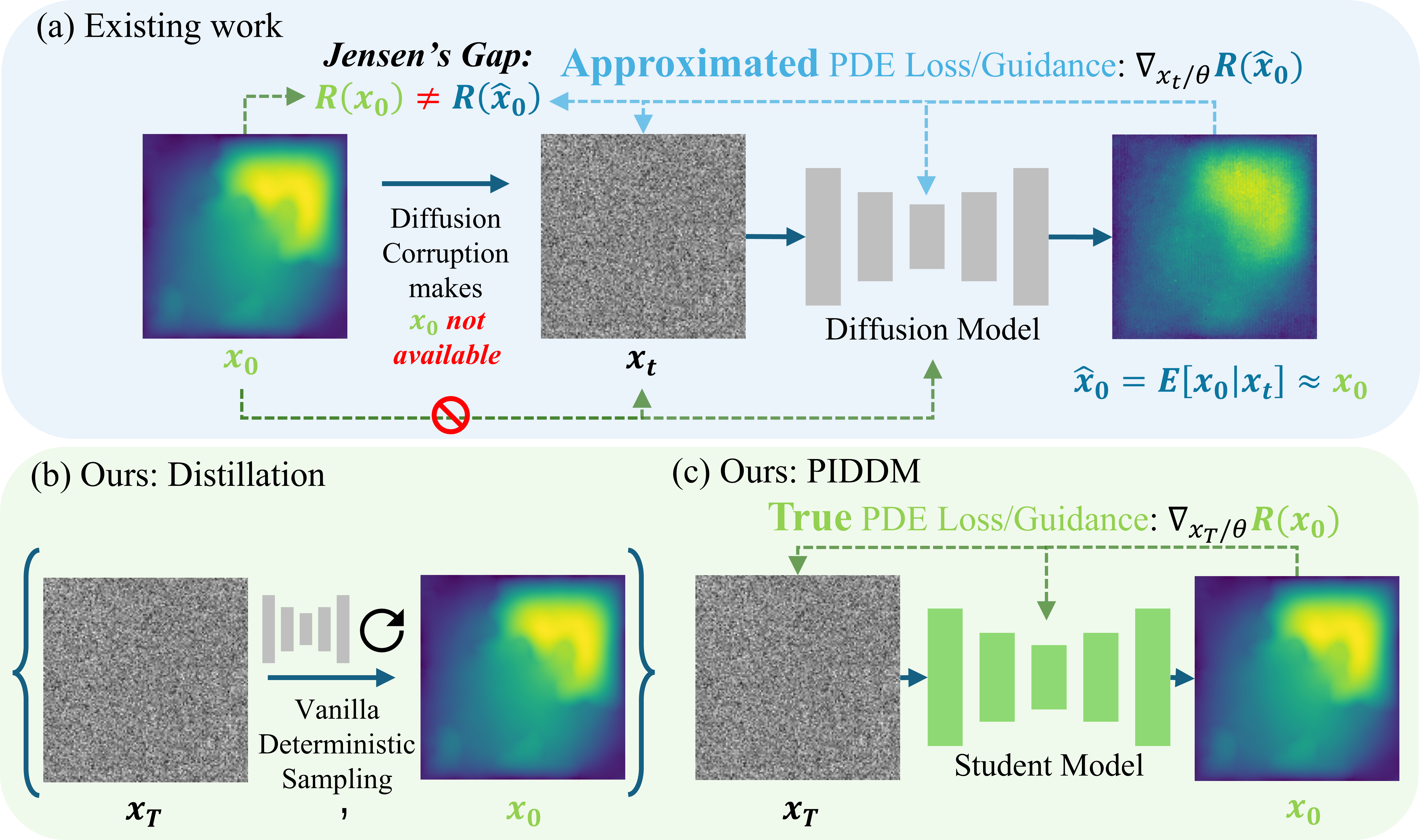
Figure 1: Illustration of physics-constrained diffusion generation and our proposed framework. (a) Existing methods huang2024diffusionpde ; cheng2025eci ; bastek2025pdim ; jacobsen2024cocogen impose PDE losses or guidance on the posterior mean $\mathbb{E}[x_{0}|x_{t}]$ in diffusion training and sampling, introducing Jensen’s Gap. (b) We propose to train and sample diffusion model using vanilla methods to generate a noise-image data paired dataset for distillation. (c) Our proposed framework distills the teacher diffusion model and directly enforces physical constraints on the final generated sample $x_{0}$, avoiding Jensen’s Gap .

Solving partial differential equations (PDEs) underpins innumerable applications in physics, biology, and engineering, spanning fluid flow davidson2015turbulence , heat transfer incropera2011heat , elasticity timoshenko1970elasticity , electromagnetism jackson1998classical , and chemical diffusion crank1975diffusion . Classical discretisation schemes such as finite-difference smith1985fem , and finite-element methods leveque2007fem provide reliable solutions, but their computational cost grows sharply with mesh resolution, dimensionality, and parameter sweeps, limiting their practicality for large-scale or real-time simulations hughes2003finite . This bottleneck has fuelled a surge of learning-based solvers that approximate or accelerate PDE solutions, from early physics-informed neural networks (PINNs) raissi2019pinn to modern operator-learning frameworks such as DeepONet lu2019deeponet , Fourier Neural Operators li2020fno and Physics-informed Neural Operator li2024pino , offering faster inference, uncertainty quantification, and seamless integration into inverse or data-driven tasks.

Among these learning-based solvers, diffusion models ho2020ddpm ; song2020score have emerged as a promising framework for generative learning of physical systems. In the context of PDEs, a diffusion model can learn the joint distribution over solution and coefficient fields ${\bm{x}}_{0}=({\bm{u}},{\bm{a}})$ from observed data, where ${\bm{a}}$ denotes input parameters satisfying boundary condition $\mathcal{B},$(e.g., material properties or initial conditions) and ${\bm{u}}$ denotes the corresponding solution satisfying the PDE system $\mathcal{F}$. Once trained, the model can generate new samples $({\bm{u}},{\bm{a}})$ from this learned distribution, enabling applications such as forward simulation (sample ${\bm{u}}$ from ${\bm{a}}$), inverse recovery (sample ${\bm{a}}$ from ${\bm{u}}$), or conditional reconstruction (recover missing parts of ${\bm{u}}$ or ${\bm{a}}$). While diffusion models perform well on conditional generation with soft, high-level constraints rombach2022ldm ; esser2024sd3 ; ho2022cfg ; chung2022dps ; ben2024dflow , PDE applications demand that outputs satisfy strict, low-level constraints specified by the operators $\mathcal{F}$ and $\mathcal{B}$.

However, enforcing PDE constraints within diffusion models is nontrivial. A core difficulty is that, at individual noise level $t$, diffusion models operate on noisy variables ${\bm{x}}_{t}$ rather than the clean physical field ${\bm{x}}_{0}$, where constraints such as $\mathcal{F}[{\bm{x}}_{0}]=0$ are defined. Once noise is added, ${\bm{x}}_{0}$ becomes inaccessible from ${\bm{x}}_{t}$, making it impractical to apply physical constraints, as shown in the left part of Fig. 1 (a). While one option is to reconstruct ${\bm{x}}_{0}$ by running the full deterministic sampling trajectory, this approach is computationally expensive, as it requires many forward passes through the diffusion model bastek2025pdim . A more common alternative is to approximate ${\bm{x}}_{0}$ with the posterior mean $\mathbb{E}[{\bm{x}}_{0}|{\bm{x}}_{t}]$, which can be efficiently computed via Tweedie’s formula bastek2025pdim ; huang2024diffusionpde ; cheng2025eci ; jacobsen2024cocogen (see right part of Fig. 1 (a)). However, this introduces a theoretical inconsistency: enforcing constraints on the posterior mean, $\mathcal{F}[\mathbb{E}[{\bm{x}}_{0}|{\bm{x}}_{t}]]$, is not equivalent to enforcing the expected constraint, $\mathbb{E}[\mathcal{F}[{\bm{x}}_{0}]|{\bm{x}}_{t}]$, due to Jensen’s inequality. This mismatch, known as the Jensen’s Gap bastek2025pdim , can lead to degraded physical fidelity. Overcoming this gap is crucial for reliable physics-constrained generation with diffusion models.

Contributions. We propose a simple yet effective framework that enforces PDE constraints in diffusion models via post-hoc distillation, enabling reliable and efficient generation under physical laws. As shown in Fig. 1 (c), our method sidesteps the limitations of existing constraint-guided diffusion-based approaches by decoupling physics enforcement from the diffusion trajectory. Our main contributions are:

• Empirical confirmation of Jensen’s Gap: We provide the first explicit empirical demonstration and quantitative analysis of the Jensen’s Gap—a fundamental discrepancy that arises when PDE constraints are imposed on the posterior mean $\mathbb{E}[{\bm{x}}_{0}|{\bm{x}}_{t}]$ at intermediate noise levels, rather than directly on the final clean sample ${\bm{x}}_{0}$.

• Theoretically sound: Our method circumvents the Jensen’s Gap by enforcing PDE constraints directly on the final generated samples. Unlike guidance-based approaches that often trade off generative quality to improve constraint satisfaction, our post-hoc distillation preserves both physical accuracy and distributional fidelity.

• Versatile and efficient inference: The distilled student model retains the full generative capabilities of the original teacher model, including physical simulation, partial observation reconstruction, and unified forward/inverse PDE solving, while supporting one-step generation for faster inference. Comprehensive experiments on various physical equations demonstrate that PIDDM outperforms existing guidance-based methods huang2024diffusionpde ; cheng2025eci ; bastek2025pdim ; jacobsen2024cocogen in both generation quality and PDE satisfaction.

2 Related Work

2.1 Diffusion Model

Diffusion models song2020score ; ho2020ddpm ; karras2022edm learn a score function, $\nabla\log p({\bm{x}}_{t})$, to reverse a predefined diffusion process, typically of the form ${\bm{x}}_{t}={\bm{x}}_{0}+\sigma_{t}\bm{\varepsilon}$. A key characteristic of diffusion models is that sampling requires iteratively reversing this process over a sequence of timesteps. This iterative nature presents a challenge for controlled generation: to guide the sampling trajectory effectively, we often need to first estimate the current denoised target $x_{0}$ in order to determine the correct guidance direction. In other words, to decide how to get there, we must first understand where we are. However, obtaining this information through full iterative sampling is computationally expensive and often impractical in optimization regime.

A practical workaround is to leverage an implicit one-step data estimate provided by diffusion models via the Tweedie’s formula efron2011tweedie , which requires only a single network forward pass:

$$\hat{{\bm{x}}}_{0}\approx\mathbb{E}[{\bm{x}}_{0}|{\bm{x}}_{t}]={\bm{x}}_{t}+\sigma_{t}^{2}\nabla\log p({\bm{x}}_{t}),$$

where $\hat{{\bm{x}}}_{0}$ denotes the final denoised sample from ${\bm{x}}_{t}$ using deterministic sampler. This gap is bridged when $t\to 0$. Although this posterior mean $\mathbb{E}[{\bm{x}}_{0}|{\bm{x}}_{t}]$ is not theoretically equivalent to the final sample obtained after full denoising, in practice, this estimate serves as a useful proxy for the underlying data and enables approximate guidance for controlled generation, without the need to complete the entire sampling trajectory.

2.2 Constrained Generation for PDE Systems

Diffusion models have demonstrated strong potential for physical-constraint applications due to their generative nature. This generative capability naturally supports the trivial task of simulating physical data and also extends to downstream applications such as reconstruction from partial observations and solving both forward and inverse problems. However, many scientific tasks require strict adherence to physical laws, often expressed as PDE constraints on the data. These constraints, applied at the sample level ${\bm{x}}$, are not easily enforced within diffusion models, which are trained to model the data distribution $p({\bm{x}})$. To address this, prior works have proposed three main strategies for incorporating physical constraints into diffusion models.

Training-time Loss Injection. PG-Diffusion shu2023physicscfg employs Classifier-Free Guidance (CFG), where a conditional diffusion model is trained using the PDE residual error as a conditioning input. However, CFG is well known to suffer from theoretical inconsistencies—specifically, the interpolated conditional score function does not match the true conditional score—which limits its suitability for enforcing precise physical constraints. To avoid this issue, PIDM bastek2025pdim introduces a loss term based on the residual evaluated at the posterior mean, $\mathbb{E}[{\bm{x}}_{0}|{\bm{x}}_{t}]$. While this approach avoids the theoretical pitfalls of CFG, the constraint is still not imposed on the actual sample ${\bm{x}}_{0}$, leading to what PIDM identifies as the Jensen’s Gap.

Sampling-time Guidance. Diffusion Posterior Sampling (DPS), used in DiffusionPDE huang2024diffusionpde and CoCoGen jacobsen2024cocogen , applies guidance during each sampling step by using the gradient of the PDE residual evaluated on the posterior mean $\mathbb{E}[x_{0}|x_{t}]$. Therefore, they inherit the Jensen’s Gap issue, as the guidance operates on an estimate of the final sample rather than the sample itself. Moreover, DPS assumes that the residual error follows a Gaussian distribution—a condition that may not hold in real-world PDE systems. Meanwhile, to support hard constraints, ECI-sampling cheng2025eci directly modifies the posterior mean $\mathbb{E}[{\bm{x}}_{0}|{\bm{x}}_{t}]$ using known boundary conditions.

Noise Prompt. Another stream of research—often called noise prompting or golden-noise optimisation—directly tunes the initial noise so that the resulting sample satisfies a target constraint ben2024dflow ; guo2024initno_goldennoise ; zhou2024golden ; wang2024silent ; mao2024lottery ; chen2024find . In the physics domain, this idea is used to minimise the true PDE residual $R({\bm{x}})$ evaluated on the final sample, rather than the surrogate residual $R(\mathbb{E}[{\bm{x}}_{0}|{\bm{x}}_{t}])$. Because the constraint is imposed on the actual output, noise prompting sidesteps the Jensen’s Gap altogether and therefore serves as a strong baseline in ECI-sampling cheng2025eci and PIDM bastek2025pdim . The main drawback is efficiency: optimising the noise requires back-propagating through the entire sampling trajectory, which is computationally expensive and prone to gradient instability.

2.3 Distillation of Diffusion Model

Sampling in diffusion models involves integrating through a reverse diffusion process, which is computationally expensive. Even with the aid of high-order ODE solvers maoutsa2020interactingode ; song2021ddim ; lu2022dpmdeterminsitc ; lu2022dpmplusplusdeterminsitc ; zhou2024fastdeterminsitc , parallel sampling shih2024paralleldeterminsitc and better training schedule karras2022edm ; nichol2021improved ; liu2023flow ; liu2023rectifiedflow ; liu2023instaflow , the process remains iterative and typically requires hundreds of network forward passes. To alleviate this inefficiency, distillation-based methods have been developed to enable one-step generation by leveraging the deterministic nature of samplers (e.g., DDIM), where the noise–data pairs become fixed. The most basic formulation, Knowledge Distillation vanilladistillation , trains a student model to replicate the teacher’s deterministic noise-to-data mapping. However, subsequent studies have shown that directly learning this raw mapping is challenging for neural networks, as the high curvature of sampling trajectories often yields noise–data pairs that are distant in Euclidean space, making the regression task ill-conditioned and hard to generalize.

To address this, recent research has proposed three complementary strategies. (1) Noise–data coupling refinement: Rectified Flow liu2023rectifiedflow distills the sampling process into a structure approximating optimal transport, where the learned mapping corresponds to minimal-cost trajectories between noise and data. InstaFlow liu2023instaflow further demonstrates that such near-optimal-transport couplings significantly ease the learning process for student models. (2) Distribution-level distillation: Rather than matching individual noise–data pairs, DMD yin2024dmd trains the student via score-matching losses that align the overall data distributions, thereby bypassing the need to regress complex mappings directly. (3) Trajectory distillation: Instead of only supervising on initial (${\bm{x}}_{T}$) and final (${\bm{x}}_{0}$) states, this approach provides supervision at intermediate states $x_{t}$ along the ODE trajectory berthelot2023tract ; zheng2023fastno ; song2023consistencymodels . This decomposition allows the student model to learn the generative process in a piecewise manner, which improves stability and sample fidelity.

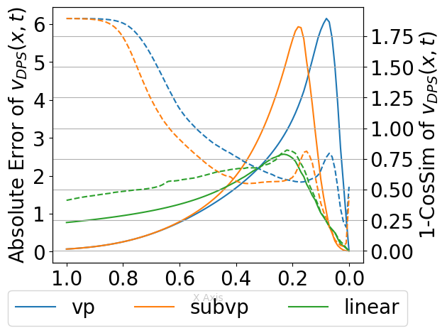
(a)

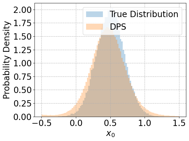
(b)

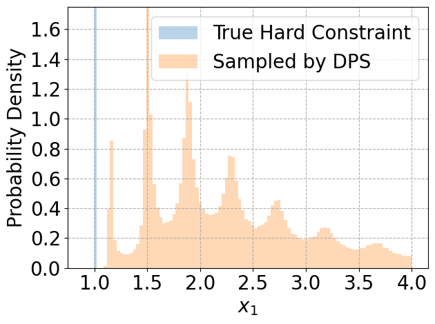
(c)

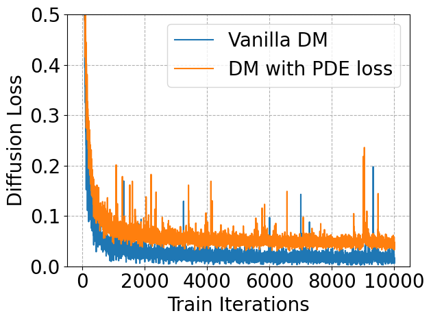
(d)

Figure 2: Empirical illustration of the Jensen’s Gap in physics-constrained diffusion models. (a) Absolute velocity error and angular discrepancy ($1-\cos(\theta)$) between Diffusion Posterior Sampling (DPS) and the ground-truth conditional ODE velocity on the MoG dataset. (b) and (c) Histograms comparing the first (unconstrained) and second (hard-constrained) dimensions of DPS-sampled MoG data against the ground truth MoG. (d) Training-time manifestation: diffusion loss comparison between vanilla training and PIDM on a Stokes Problem dataset.

3 Problem Setup: Jensen’s Gap in Diffusion Model with PDE constraints

In scientific machine learning, there exist many hard and low-level constraints that are mathematically strict and non-negotiable leveque1992numerical ; hansen2023learning ; mouli2024using ; saad2022guiding , which are hard to satisfy via standard diffusion models (han2025can, ; han2024feature, ). In this section, we will discuss how existing works impose these constraints in diffusion-generated data, and the Jensen’s Gap gao2017jensen ; bastek2025pdim ; huang2024diffusionpde it introduces.

3.1 Preliminaries on Physics constraints

Physics constraints are typically expressed as a partial differential equation (PDE) $\mathcal{F}$ defined over a solution domain $\Omega\subset\mathbb{R}^{d}$, together with a boundary condition operator $\mathcal{B}$ defined on the coefficient domain $\Omega^{\prime}$:

$$\mathcal{F}[\mathbf{u}(\bm{\xi})]=0\text{ for }\bm{\xi}\in\Omega,\quad\mathcal{B}[\mathbf{a}(\bm{\xi^{\prime}})]=0\text{ for }\bm{\xi^{\prime}}\in\Omega^{\prime}.$$ (1)

In practice, the domain $\Omega$ and $\Omega^{\prime}$ is discretized into a uniform grid, typically of size $H\times W$, and the field ${\bm{u}}$ and ${\bm{a}}$ are evaluated at those grid points to produce the observed data ${\bm{x}}_{0}=({\bm{u}},{\bm{a}})$, where diffusion models are trained to learn the joint distribution $p({\bm{x}}_{0})=p(({\bm{u}},{\bm{a}}))$. While PINNs raissi2019pinn model the mapping $\bm{\xi}\,,\bm{\xi^{\prime}}\mapsto(\mathbf{u}(\bm{\xi}),\mathbf{a}(\bm{\xi^{\prime}}))$ with differentiable neural networks to enable automatic differentiation paszke2019pytorch ; abadi2016tensorflow , grid-based approaches commonly approximate the differential operators in $\mathcal{F}$ via finite difference methods smith1985fem ; leveque2007fem . To quantify the extent to which a generated sample ${\bm{x}}_{0}$ violates the physical constraints, the physics residual error in often defined by:

$$\mathcal{R}({\bm{x}}_{0})=\mathcal{R}(({\bm{u}},{\bm{a}})):=\big{[}\mathcal{F}[{\bm{u}}],\mathcal{B}[{\bm{a}}]\big{]}^{\top}$$ (2)

Here, $\mathcal{R}({\bm{x}})$ measures the discrepancy between the sample ${\bm{x}}$ and the expected PDE $\mathcal{F}$ and boundary conditions $\mathcal{B}$. The physics residual loss is often defined by the squared norm of this physics residual error, i.e., $\|\mathcal{R}({\bm{x}})\|^{2}$.

3.2 Imposing PDE constraints in Diffusion Models

The physical constraints $\mathcal{R}$ are often defined on the clean field ${\bm{x}}_{0}$, while during training or sampling of the diffusion model, the model only observes the noisy state ${\bm{x}}_{t}$. Therefore, it is intractable to make direct optimization or controlled generation based on the physical residual loss $\mathcal{R}({\bm{x}}_{0})$. A practical workaround, therefore, is to evaluate the constraint on an estimate of ${\bm{x}}_{0}$ from ${\bm{x}}_{t}$, and a common choice is to use the estimated posterior mean: $\mathbb{E}[{\bm{x}}_{0}\mid{\bm{x}}_{t}]$ based on the score network in diffusion model (bastek2025pdim, ; huang2024diffusionpde, ). As a simplified example, consider the forward process defined as ${\bm{x}}_{t}={\bm{x}}_{0}+\sigma_{t}\bm{\epsilon}$, where $\sigma_{t}$ denotes the noise level at time $t$ and $\bm{\epsilon}\sim\mathcal{N}(0,\mathbf{I})$ is standard Gaussian noise. Then, the posterior mean can be efficiently estimated via Tweedie’s formula:

$$\hat{{\bm{x}}}_{\theta}({\bm{x}}_{t},t):={\bm{x}}_{t}+\sigma_{t}^{2}s_{\theta}({\bm{x}}_{t},t)\approx{\bm{x}}_{t}+\sigma_{t}^{2}\nabla\log p({\bm{x}}_{t})\approx\mathbb{E}[{\bm{x}}_{0}\mid{\bm{x}}_{t}],$$ (3)

where $s_{\theta}$ is a learned score function approximating the gradient of the log-density (see Appendix A.2 for the derivations for the general diffusion process). Leveraging this approximation, several existing works incorporate PDE constraints by evaluating the PDE residual operator $\mathcal{R}$ on $\hat{{\bm{x}}}_{\theta}({\bm{x}}_{t},t)$. For instance, PIDM bastek2025pdim integrates PDE constraints into diffusion model at training time by augmenting the standard diffusion objective with an additional PDE residual loss $\mathcal{R}(\hat{{\bm{x}}}_{\theta}({\bm{x}}_{t},t))$. Similarly, at inference time, DiffusionPDE huang2024diffusionpde and CoCoGen jacobsen2024cocogen employ diffusion posterior sampling (DPS) chung2022dps , guiding each intermediate sample ${\bm{x}}_{t}$ using the gradient $\nabla_{{\bm{x}}}\mathcal{R}(\hat{{\bm{x}}}_{\theta}({\bm{x}}_{t},t))$. On the other hand; ECI-sampling cheng2025eci directly projects hard constraints onto the posterior mean at each DDIM step using a correction operator (more detailed discussion on their implementations can be found in Appendix  C.4). While these pioneering methods have been demonstrated to be effective in enforcing PDE constraints within diffusion models, they still suffer a theoretical inconsistency: PDE constraints are enforced on the posterior mean approximation $\mathbb{E}[{\bm{x}}_{0}|{\bm{x}}_{t}]$, which is not equivalent to the constraints on the true generated data ${\bm{x}}_{0}$ due to Jensen’s inequality:

$$\mathcal{R}(\mathbb{E}[{\bm{x}}_{0}|{\bm{x}}_{t}])\neq\mathbb{E}[\mathcal{R}({\bm{x}}_{0})|{\bm{x}}_{t}].$$ (4)

This discrepancy is commonly referred to as the Jensen’s Gap bastek2025pdim ; huang2024diffusionpde ; gao2017jensen . To mitigate this issue, PIDM and DiffusionPDE heuristically down-weight PDE constraints at early denoising steps (large $t$) in training and sampling, respectively, where Jensen’s Gap is pronounced, and emphasize them near $t\to 0$, where the posterior mean approximation improves. ECI-sampling introduces stochastic resampling steps wang2025resample to project theoretically inconsistent intermediate samples back toward their correct distribution. Although these methods provide partial practical improvements, they remain fundamentally limited by their ad hoc nature—neither resolves the underlying theoretical gap nor guarantees rigorous physical constraint satisfaction in generated outputs.

3.3 Demonstration of the Jensen’s Gap

To better illustrate the presence of Jensen’s gap and its negative effect, we conduct experiments on two synthetic datasets: a Mixture-of-Gaussians (MoG) dataset and a Stokes Problem dataset.

Sampling-time Jensen’s Gap. We demonstrate the sampling-time Jensen’s Gap using the Mixture-of-Gaussians (MoG) dataset, where the score function is analytically tractable, allowing us to isolate the effect of the diffusion process without interference from training error. The MoG is constructed in 2D: the first dimension follows a bimodal Gaussian distribution, while the second dimension encodes a discrete latent variable that serves as a hard constraint. Concretely, the joint distribution is defined as a mixture of two Gaussians, each supported on a distinct horizontal line:

$$p(x_{0})=0.5\cdot\,\mathcal{N}(x_{1};-1,\sigma^{2})\cdot\delta(x_{2}+1)+0.5\cdot\,\mathcal{N}(x_{1};+1,\sigma^{2})\cdot\delta(x_{2}-1),$$ (5)

where $\delta(\cdot)$ denotes the Dirac delta function and $\sigma=0.2$. To examine the impact of Jensen’s Gap during sampling, we compare Diffusion Posterior Sampling (DPS) chung2022dps which uses a latent code to guide the generation, with the ground-truth conditional ODE trajectory derived analytically. We evaluate three representative diffusion processes: Variance-Preserving (VP) ho2020ddpm , Sub-VP song2020score , and Linear liu2023flow , and compare their velocity field during the inference for characterizing Jensen’s Gap. To quantify amplitude errors, we compute the mean absolute error (MAE) and angular error between the DPS-predicted velocity field $v_{\text{DPS}}(x,t)$ and the ground-truth velocity $v_{\text{GT}}(x,t)$: We observe that both of these errors of DPS are significantly elevated at intermediate timesteps and only diminish as $t\to 0$, as shown in Fig.2(a). Although DPS achieves accurate sampling in the unconstrained dimension (Fig.2(b)), it fails to respect the hard constraint in the constrained dimension (Fig. 2(c)).

Training-time Jensen’s Gap. To examine the Jensen’s Gap during training, we use the synthetic Stokes Problem dataset as the target modeling distribution $p_{\text{Stokes}}$. The diffusion model ${\bm{v}}_{\theta}$ adopts a Fourier Neural Operator (FNO) li2020fno architecture, and the diffusion process follows a standard linear noise schedule lipman2023flow ; liu2023rectifiedflow ; liu2023instaflow . Further details of the dataset and training configuration are provided in Appendices B and C. We take PIDM bastek2025pdim as an example, which explicitly adds the PDE loss $\mathcal{R}(\hat{\bm{x}}_{\theta}({\bm{x}}_{t},t))$ to the diffusion loss, and compare its performance with the standard diffusion training. To evaluate generative performance, we track the diffusion loss, which theoretically serves as an evidence lower bound (ELBO) ho2020ddpm ; kingma2013vae ; dayan1995helmholtz ; rezende2014stochastic ; efron2011tweedie . The comparison results are shown in Fig. 2(d), revealing a significant increase in diffusion loss when the PDE residual loss is incorporated. This suggests that the PDE residual loss does not help better shape the data distribution that satisfies the PDE constraints. This observation also corroborates findings from PIDM bastek2025pdim , which identified that residual supervision on the posterior mean can create “a conflicting objective between the data and residual loss”, where the data loss represents the original diffusion training objective. These results provide further evidence for the existence of the Jensen’s Gap in training, as enforcing constraints on $\mathbb{E}[{\bm{x}}_{0}|{\bm{x}}_{t}]$ may interfere with maximizing the likelihood of the true data distribution.

4 Method: Physics-Informed Distillation of Diffusion Models

Algorithm 1 PIDDM Training: Physics-Informed Distillation.

1:Teacher Model ${\bm{v}}_{\theta}({\bm{x}},t)$, Student Model $d_{\bm{\theta}^{\prime}}$, Batch Size $B$, Steps $N_{s}$, Step Size $\mathrm{d}t{=}1/N_{s}$, Physics Residual Error $\mathcal{R}$, Loss Weight $\lambda_{\text{train}}$, Learning Rate $\eta_{\text{train}}$

2:repeat

3:  Sample $\bm{\epsilon}_{1:B}\stackrel{{\scriptstyle\text{i.i.d.}}}{{\sim}}{\mathcal{N}}(\mathbf{0},\mathbf{I})$; ${\bm{x}}_{T}\leftarrow\bm{\epsilon}_{1:B}$

4:  For $t=T{-}\mathrm{d}t,\dots,0$ ${\bm{x}}_{t}\leftarrow{\bm{x}}_{t{+}\mathrm{d}t}-{\bm{v}}_{\theta}({\bm{x}}_{t{+}\mathrm{d}t},t{+}\mathrm{d}t)\,\mathrm{d}t$$\triangleright$ Sampling Phase

5:  ${\bm{x}}_{\text{pred}}\leftarrow d_{\bm{\theta}^{\prime}}(\bm{\epsilon}_{1:B})$

6:  $\mathcal{L}\leftarrow\tfrac{1}{B}(\bigl{\|}{\bm{x}}_{\text{pred}}-{\bm{x}}_{0}\bigr{\|}^{2}+\lambda_{\text{train}}\bigl{\|}\mathcal{R}(\hat{\bm{x}})\bigr{\|}^{2})$ $\triangleright$ Distillation Phase

7:  $\theta^{\prime}\leftarrow\theta^{\prime}-\eta_{\text{train}}\nabla_{\theta^{\prime}}\mathcal{L}$

8:until Converged

In the previous Section 3, we have demonstrated the existence of the Jensen’s Gap when incorporating physical constraints into diffusion training and sampling, as observed in prior works. To address this issue, we propose a distillation-based framework that theoretically bypasses the Jensen’s Gap. In specific, instead of enforcing constraints on the posterior mean during the diffusion process which introduces a trade-off with generative accuracy, we apply physical constraints directly to the final generated samples in a post-hoc distillation stage.

4.1 Diffusion Training

To decouple physical constraint enforcement from the diffusion process itself, we first conduct standard diffusion model training using its original denoising objective, without adding any constraint-based loss. To achieve smoother sampling trajectory which benefits later noise-data distillation liu2023rectifiedflow ; liu2023instaflow , we adopt a linear diffusion process and apply the ${\bm{v}}$-prediction parameterization liu2023rectifiedflow ; lipman2023flow ; liu2023instaflow ; cheng2025eci ; esser2024sd3 , which is commonly referred to as a flow model. In specific, the training objective is defined as:

$$\mathcal{L}(\bm{\theta})=\mathbb{E}_{t\sim U(0,1),{\bm{x}}_{0}\sim p({\bm{x}}_{0}),\mathbf{\epsilon}\sim cN(\mathbf{0,\mathbf{I}})}\left\|({\bm{v}}_{\bm{\theta}}({\bm{x}}_{t},t)-(\bm{\epsilon}-{\bm{x}}_{0})\right\|^{2},\quad{\bm{x}}_{t}=(1-t){\bm{x}}_{0}+t\bm{\epsilon},$$ (6)

where $p({\bm{x}}_{0})$ is the distribution of joint data containing both solution and coefficient fields ${\bm{x}}=({\bm{u}},{\bm{a}})$, $\bm{\epsilon}$ is sampled from a standard Gaussian distribution, and ${\bm{v}}_{\bm{\theta}}$ is the neural network as the diffusion model. This formulation allows the model to learn to reverse the diffusion process without entangling it with physical supervision, thereby preserving generative fidelity.

4.2 Imposing PDE Constraints in Distillation

Algorithm 2 PIDDM Inference: Physics Data Simulation

1:Input Student Model $d_{\bm{\theta^{\prime}}}$, Physics Residual Error $\mathcal{R}$, Refinement Step Number $N_{f}$, Refinement Step Size $\eta_{\text{ref}}$, Latent Noise $\bm{\epsilon}\sim\mathcal{N}(\mathbf{0},\mathbf{I})$.

2:For $i=1,\dots,N_{f}:$ $\bm{\epsilon}\leftarrow\bm{\epsilon}-\eta_{\text{ref}}\nabla_{\bm{\epsilon}}\|\mathcal{R}(d_{\bm{\theta^{\prime}}}(\bm{\epsilon}))\|^{2}$ $\triangleright$ PDE refinement step (optional).

3:Output $d_{\bm{\theta^{\prime}}}(\bm{\epsilon})$

Algorithm 3 PIDDM Inference for Forward/Inverse/Reconstruction

1:Input Student Model $d_{\bm{\theta^{\prime}}}$, Physics Residual Error $\mathcal{R}$, Optimization Iteration $N_{o}$, Step Size $\eta_{\text{infer}}$, Observation ${\bm{x}}^{\prime}$, Observation Mask $M$, Loss Weight $\lambda_{\text{infer}}$, Latent Noise $\bm{\epsilon}\sim\mathcal{N}(\mathbf{0},\mathbf{I})$.

2:for $i=1,\dots,N_{o}$ do

3:  ${\bm{x}}_{\text{mix}}\leftarrow{\bm{x}}^{\prime}\odot M+d_{\bm{\theta^{\prime}}}(\bm{\epsilon})\odot(1-M)$

4:  $\bm{\epsilon}\leftarrow\bm{\epsilon}-\eta_{\text{infer}}\nabla_{\bm{\epsilon}}[\left\|(d_{\bm{\theta^{\prime}}}(\bm{\epsilon})-{\bm{x}}^{\prime})\odot M\right\|^{2}+\lambda_{\text{infer}}\left\|\mathcal{R}({\bm{x}}_{\text{mix}})\right\|^{2}]$

5:end for

6:${\bm{x}}\leftarrow{\bm{x}}^{\prime}\odot M+d_{\bm{\theta^{\prime}}}(\bm{\epsilon})\odot(1-M)$

7:Output ${\bm{x}}$

After training the teacher diffusion model using the standard denoising objective, we proceed to the distillation stage, where we transfer its knowledge to a student model designed for efficient one-step generation. Crucially, this post-hoc distillation stage is where we impose PDE constraints, thereby avoiding the Jensen’s Gap observed in prior works that apply constraints during diffusion training or sampling. This distillation process is guided by two complementary objectives: (1) learning to map a noise sample to the final generated output predicted by the teacher model, and (2) enforcing physical consistency on this output via PDE residual minimization. Concretely, we begin by sampling a noise input $\varepsilon\sim\mathcal{N}(0,\mathbf{I})$ and generate a target sample $x_{0}$ using the pre-trained teacher model via deterministic integration of the reverse-time ODE:

$${\bm{x}}_{t-\mathrm{d}t}={\bm{x}}_{t}-{\bm{v}}_{\bm{\theta}}({\bm{x}}_{t},t)\,\mathrm{d}t,$$ (7)

which proceeds from $t=1$ to $t=0$ using a fixed step size $dt$. This yields a paired noise-data dataset $\mathcal{D}=\{\bm{\epsilon},{\bm{x}}_{0}\}$ for distillation, as shown in Fig. 1 (b). Then a student model $d_{\bm{\theta}^{\prime}}(\bm{\epsilon})$ is trained to predict ${\bm{x}}_{0}$ in one step, as shown in Fig. 1 (c). Meanwhile, to enforce physical consistency, we evaluate the physics residual error on the output ${\bm{x}}=d_{\bm{\theta}^{\prime}}(\varepsilon)$, i.e., $\left\|\mathcal{R}({\bm{x}})\right\|^{2}$. The overall training objective is:

$$\mathcal{L}_{\text{total}}=\mathcal{L}_{\text{PDE}}+\lambda\mathcal{L}_{\text{sample}}=\mathbb{E}_{(\bm{\epsilon},{\bm{x}}_{0})\sim\mathcal{D}}\left[\left\|d_{\bm{\theta}^{\prime}}(\bm{\epsilon})-{\bm{x}}_{0}\right\|^{2}\right]+\lambda_{\text{train}}\left\|\mathcal{R}({\bm{x}})\right\|^{2},$$ (8)

where $\lambda_{\text{train}}$ is a tunable hyperparameter that balances generative fidelity and physical constraint satisfaction. The optimization is repeated until convergence, as described in Algorithm 1. The most relevant prior work is vanilla knowledge distillation vanilladistillation , which trains a student model to map noise to data using pairs sampled via deterministic samplers from a teacher diffusion model. However, this mapping is difficult to learn due to the high curvature of sampling trajectories, which produces noise–data pairs that are distant in Euclidean space liu2023instaflow . To address this, we adopt a linear diffusion process lipman2023flow ; liu2023rectifiedflow , which yields smoother trajectories and enhances learnability. Beyond this setup, we further evaluate more advanced distillation strategies, including Rectified Flow liu2023instaflow and Distribution Matching Distillation yin2024dmd , which improve coupling and distribution alignment, respectively (see Table 3 for more details).

Table 1: Generative metrics on various PDE problems. The PDE error means the MSE of the evaluated physics residual error. The best results are in bold and the second best are underlined.

Dataset	Metric	PIDDM-1	PIDDM-ref	ECI	DiffusionPDE	D-Flow	PIDM	Vanilla
Darcy	MMSE ($\times 10^{-2}$)	0.112	0.037	0.153	0.419	0.129	0.515	0.108
	SMSE ($\times 10^{-2}$)	0.082	0.002	0.103	0.163	0.085	0.368	0.069
	PDE Error ($\times 10^{-4}$)	0.226	0.148	1.582	1.071	0.532	1.236	1.585
	NFE ($\times 10^{3}$)	0.001	0.080	0.500	0.100	5.000	0.100	0.100
Poisson	MMSE ($\times 10^{-2}$)	0.162	0.113	0.183	0.861	0.172	0.948	0.150
	SMSE ($\times 10^{-2}$)	0.326	0.274	0.291	0.483	0.475	0.701	0.353
	PDE Error ($\times 10^{-9}$)	0.073	0.050	2.420	1.270	0.831	1.593	2.443
	NFE ($\times 10^{3}$)	0.001	0.080	0.500	0.100	5.000	0.100	0.100
Burger	MMSE ($\times 10^{-2}$)	0.152	0.012	0.294	0.064	0.305	0.948	0.264
	SMSE ($\times 10^{-2}$)	0.133	0.101	0.105	0.103	0.207	0.701	0.114
	PDE Error ($\times 10^{-3}$)	0.466	0.174	1.572	1.032	0.730	1.593	1.334
	NFE ($\times 10^{3}$)	0.001	0.080	0.500	0.100	5.000	0.100	0.100

4.3 Downstream Tasks

Our method naturally supports one-step generation of physically-constrained data, jointly producing both coefficient and solution fields. Beyond this intrinsic functionality, it also retains the flexibility of the teacher diffusion model, enabling various downstream tasks such as forward and inverse problem solving, and reconstruction from partial observations. Compared to the teacher model, our method achieves these capabilities with improved computational efficiency and stronger physical alignment.

Generative Modeling. In our setting, generative modeling aims to sample physically consistent pairs ${\bm{x}}_{0}=({\bm{u}},{\bm{a}})$—representing solution and coefficient fields—from a learned distribution that satisfies the underlying PDE system. Our student model inherently supports this task through efficient one-step generation: given a latent variable $\bm{\epsilon}\sim\mathcal{N}(\mathbf{0},\mathbf{I})$, the model directly outputs a sample ${\bm{x}}_{0}=d_{\bm{\theta^{\prime}}}(\bm{\epsilon})$ that approximates a valid solution–coefficient pair. Beyond this default mode, we introduce an optional refinement stage based on constraint-driven optimization (Algorithm 2), which further reduces the physics residual by updating $\bm{\epsilon}$ via gradient descent. This strategy is inspired by noise prompting techniques ben2024dflow ; guo2024initno_goldennoise , which optimize the final generated sample with respect to the initial noise. However, unlike those methods—which require backpropagation through the entire sampling trajectory and thus suffer from high computational cost and issues like gradient vanishing or explosion—our refinement operates efficiently in a one-step setting. While optional, this mechanism offers an additional degree of control, which is particularly valuable in scientific applications that demand strict physical consistency leveque1992numerical ; hansen2023learning ; mouli2024using ; saad2022guiding .

Forward/Inverse Problem and Reconstruction. PIDDM handles all downstream problems as conditional generation over the joint field ${\bm{x}}=({\bm{u}},{\bm{a}})$. Forward inference draws ${\bm{u}}$ from known ${\bm{a}}$; inverse inference recovers ${\bm{a}}$ from observed ${\bm{u}}$; reconstruction fills in missing entries of $({\bm{u}},{\bm{a}})$ given a partial observation ${\bm{x}}^{\prime}$. We solve this via optimization-based inference on the latent variable $\bm{\varepsilon}$, using the same student model $d_{\bm{\theta}^{\prime}}$ as in generation, as described in Algorithm. 3.. Let ${\bm{x}}=d_{\bm{\theta}^{\prime}}(\bm{\varepsilon})$ denote the generated sample, and let $M$ be a binary observation mask indicating the known entries in ${\bm{x}}^{\prime}$ with respect to ${\bm{x}}$. To ensure hard consistency with observed values (e.g., boundary conditions $\mathcal{B}$), we define a mixed sample by injecting observed entries into the generated output, following ECI-sampling cheng2025eci and then update $\varepsilon$ by descending the gradient of a combined objective:

$$\mathcal{L}_{\text{total}}=\left\|\left({\bm{x}}-{\bm{x}}^{\prime}\right)\odot M\right\|^{2}+\lambda\left\|\mathcal{R}({\bm{x}}_{\text{mix}})\right\|^{2},\quad{\bm{x}}_{\text{mix}}={\bm{x}}^{\prime}\odot M+{\bm{x}}\odot(1-M).$$ (9)

Interestingly, we also find that applying this masking not only enhances hard constraints on $\mathcal{B}$, but also improves satisfaction of $\mathcal{F}$, as demonstrated in our ablation study in Table 3. Classical inverse solvers li2020fno ; li2024pino ; lu2019deeponet ; raissi2019pinn learn a deterministic map ${\bm{u}}\!\mapsto\!{\bm{a}}$ and therefore require full observations of ${\bm{a}}$ to evaluate $\mathcal{F}[{\bm{u}},{\bm{a}}]=0$, a condition rarely met in practice. DiffusionPDE huang2024diffusionpde relaxes this by sampling missing variables, but enforces physics on the posterior mean, i.e. $\mathcal{F}\!\bigl{[}\mathbb{E}[{\bm{x}}_{0}\!\mid\!{\bm{x}}_{t}]\bigr{]}$, and thus suffers from the Jensen’s Gap. Our method avoids this inconsistency by imposing constraints directly on the final sample $\mathcal{F}[{\bm{x}}_{0}]$, yielding more reliable and physically consistent inverse solutions.

5 Experiments

Experiment Setup. We consider three widely used PDE benchmarks in main text: Darcy flow, Poisson equation, and Burger’s equation. Each dataset contains paired solution and coefficient fields defined on a $128\times 128$ grid. All of these data are readily accessible from FNO li2020fno and DiffusionPDE huang2024diffusionpde . We also provide results on other benchmarks in Appendix. D. We consider ECI cheng2025eci , DiuffsionPDE huang2024diffusionpde , D-Flow cheng2025eci ; ben2024dflow , PIDM bastek2025pdim and vanilla diffusion models as baseline methods, where we put the detailed implementation in Appendix. C.4. We follow ECI-sampling cheng2025eci to use FNO as both of the teacher diffusion models and the student distillation model. We put full specification of our experiment setup in Appendix. C.

To quantitatively evaluate performance, we report MMSE and SMSE following prior work cheng2025eci ; kerrigan2023functional : MMSE measures the mean squared error of the sample mean; SMSE evaluates the error of the sample standard deviation, reflecting the quality of distribution modeling. PDE Error quantifies the violation of physical constraints using the physics residual error $\lvert\mathcal{R}({\bm{x}})\rvert^{2}$. The number of function evaluations (NFE) reflects computational cost during inference. For downstream tasks, we additionally report MSE on solution, or coefficient fields, or both of them, depending on the setting.

5.1 Empirical Evaluations

PIDDM samples the joint field $({\bm{u}},{\bm{a}})$, enabling forward (${\bm{u}}|{\bm{a}}$), inverse (${\bm{a}}|{\bm{u}}$), and reconstruction (partial ${\bm{u}},{\bm{a}}$) tasks (Sec. 4.3). DiffusionPDE huang2024diffusionpde reports only reconstruction MSE, while ECI-sampling cheng2025eci and PIDM bastek2025pdim cover at most one task, limited to either unconditional generation or forward solving. For a fair comparison, we evaluate all methods on all three tasks using both reconstruction error and PDE residual, providing a unified view of generative quality and physical fidelity.

Generative Tasks. We first evaluate the generative performance of our method across three representative PDE systems: Darcy, Poisson, and Burgers’ equations. As shown in Table 1, our one-step model (PIDDM-1) achieves competitive MMSE and SMSE scores while maintaining extremely low computational cost (1 NFE). Notably, PIDDM-1 already surpasses all prior methods that incorporate physical constraints during training or sampling, such as PIDM and DiffusionPDE, ECI-sampling, which suffer from the Jensen’s Gap and only exhibit marginal improvements over vanilla diffusion baselines. Our optional refinement stage (PIDDM-ref) further reduces both statistical errors and physical PDE residuals, outperforming all baselines. Meanwhile, ECI—which only enforces hard constraints on boundary conditions—achieves moderate improvements but remains less effective on field-level physical consistency. Although D-Flow theoretically enforces physical constraints throughout the trajectory, it requires thousands of NFEs and often suffers from gradient instability.

Forward/Inverse Solving and Reconstruction. We further demonstrate the versatility of our method in forward and inverse problem solving on the Darcy dataset. Since the original PIDM bastek2025pdim implementation addresses only unconditional generation, we pair it with Diffusion Posterior Sampling (DPS) chung2022dps to extend it to downstream tasks (forward, inverse, and reconstruction). Following the test protocol of D-Flow, we apply inference-time optimization over the initial noise to match given observations while satisfying physical laws. As shown in Table 2, our method (PIDDM) achieves the best results across all metrics—including MSE and PDE error—while being significantly more efficient than D-Flow, which requires 5000 function evaluations. Compared to ECI and DiffusionPDE, our method yields lower residuals and better predictive accuracy, reflecting its superior handling of physical and observational constraints jointly.

Table 2: Evaluation on various downstream tasks on Darcy Datasets. The PDE error means the MSE of the evaluated physics residual error. The best results are in bold.

Task	Metric	PIDDM	ECI	DiffusionPDE	D-Flow	PIDM
Forward	MSE ($\times 10^{-1}$)	0.316	0.776	0.691	0.539	0.380
	PDE Error ($\times 10^{-4}$)	0.145	1.573	1.576	0.584	1.248
	NFE ($\times 10^{3}$)	0.080	0.500	0.100	5.000	0.100
Inverse	MSE ($\times 10^{-1}$)	0.236	0.545	0.456	0.428	0.468
	PDE Error ($\times 10^{-4}$)	0.126	1.505	1.402	0.438	1.113
	NFE ($\times 10^{3}$)	0.080	0.500	0.100	5.000	0.100
Reconstruct	Coef MSE ($\times 10^{-1}$)	0.128	0.395	0.240	0.158	0.179
	Sol MSE ($\times 10^{-1}$)	0.102	0.219	0.143	0.125	0.147
	PDE Error ($\times 10^{-4}$)	0.143	1.205	1.239	0.605	1.240
	NFE ($\times 10^{3}$)	0.080	0.500	0.100	5.000	0.100

5.2 Ablation Studies

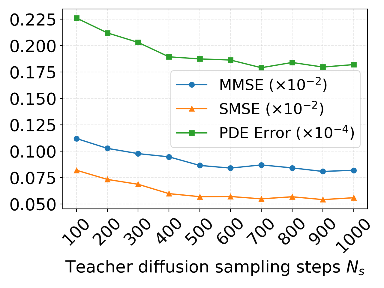
(a)

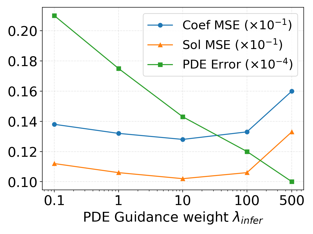
(b)

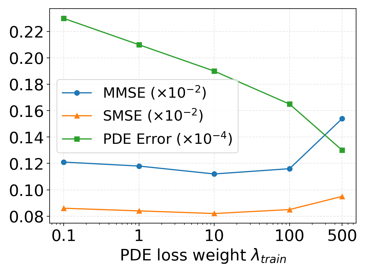
(c)

Figure 3: Ablation studies on the effect of several factors on the performance of PIDDM on Darcy dataset. (a), (b) and (c) refer to the effect of the $N_{s}$, $\lambda_{\text{train}}$ and $\lambda_{\text{infer}}$, respectively.

To better understand the effect of key design choices in PIDDM, we perform ablations on five factors: teacher sampling steps $N_{s}$; distillation weight $\lambda_{\text{train}}$; inference weight $\lambda_{\text{infer}}$; diffusion schedule (VP, sub-VP, linear); and advanced distillation variants (Rectified Flow, DMD). Figure 3 presents three key ablation studies on the Darcy dataset. Panel (a) shows that increasing the teacher model’s sampling steps $N_{s}$ consistently improves both generative quality and physical alignment, as reflected by lower MMSE, SMSE, and PDE residuals of the distilled student—highlighting the importance of high-fidelity supervision. Panels (b) and (c) examine the impact of the PDE loss weight during distillation and inference, respectively. A moderate weight significantly reduces the PDE residual, but an overly large weight leads to a slight degradation in MMSE and SMSE. This trade-off arises from the numerical approximation errors introduced by finite difference discretizations. Overall, these results suggest that while stronger PDE guidance improves physical consistency, excessively large weights can harm statistical fidelity due to discretization-induced bias. These ablation studies show potential limitations such as reliance on a pre-trained teacher model, and sensitivity to the choice of PDE loss weight.

Table 3: Generative metrics on various downstream tasks on Darcy Datasets using Different Distillation. PIDDM: Our method, $\text{PIDDM}_{\text{RF-1}}$: reflowing liu2023instaflow for once, $\text{PIDDM}_{\text{RF-2}}$: reflowing liu2023instaflow for twice, and $\text{PIDDM}_{\text{DMD}}$: yin2024dmd . $\text{PIDDM}_{\text{wo HC}}$ refers to the ablation study when not using hard-constraints 9 in PIDDM inference. $\text{PIDDM}_{\text{VP}}$ and $\text{PIDDM}_{\text{sub-VP}}$ refers the ablation study on vp and sub-vp diffusion process. The PDE error means the MSE of the evaluated physics residual error. The best results are in bold.

Dataset	Metric	PIDDM	$\text{PIDDM}_{\text{RF-1}}$	$\text{PIDDM}_{\text{RF-2}}$	$\text{PIDDM}_{\text{DMD}}$	$\text{PIDDM}_{\text{wo hc}}$	$\text{PIDDM}_{\text{VP}}$	$\text{PIDDM}_{\text{sub-VP}}$
Forward	MSE ($\times 10^{-1}$)	0.316	0.278	0.127	0.255	0.705	0.398	0.372
	PDE Error ($\times 10^{-4}$)	0.145	0.129	0.098	0.134	0.354	0.154	0.157
Inverse	MSE ($\times 10^{-1}$)	0.236	0.195	0.136	0.188	0.503	0.284	0.271
	PDE Error ($\times 10^{-4}$)	0.115	0.126	0.079	0.121	0.321	0.143	0.139
Reconstruct	Coef MSE ($\times 10^{-1}$)	0.128	0.107	0.913	0.954	0.294	0.133	0.138
	Sol MSE ($\times 10^{-1}$)	0.102	0.084	0.063	0.073	0.239	0.127	0.119
	PDE Error ($\times 10^{-4}$)	0.143	0.118	0.085	0.104	0.464	0.159	0.158

We also explore whether more sophisticated distillation strategies can improve the quality of the student model. As shown in Table 3, advanced techniques such as Rectified Flow (RF-1, RF-2) and Distribution Matching Distillation (DMD) yield better MMSE and SMSE than the vanilla baseline, while maintaining competitive PDE residuals. This suggests that better coupling of noise and data trajectories in distillation can reduce the trade-off between sample quality and constraint alignment. Notably, RF-2 achieves the best overall performance across forward and inverse tasks. Besides, we analyze the effect of imposing hard constraints during downstream inference. Following the strategy inspired by ECI-sampling, we directly replace the masked entries in the generated sample with observed values before computing the PDE residual. This ensures that the known information is preserved when evaluating physical consistency. As shown in Table 3, applying this hard constraint significantly improves PDE residual across all tasks. We also validate our design on using linear diffusion process,

6 Conclusion and Future Work

Method. We introduce PIDDM, a lightweight yet effective post-hoc distillation framework that enables diffusion models for physics-constrained generation. Concretely, we first train a standard diffusion model and then distill it into a student model by directly enforcing PDE constraints on the final output. In contrast to existing methods that impose constraints on the posterior mean $\mathbb{E}[{\bm{x}}_{0}\mid{\bm{x}}_{t}]$, leading to a mismatch known as the Jensen’s Gap which leads to a trade-off between generative quality and constraint satisfaction, PIDDM applies constraints on the actual sample ${\bm{x}}_{0}$, ensuring physics consistency without sacrificing distributional fidelity.

Empirical Findings. We provide the first empirical illustrations of the Jensen’s Gap in both diffusion training and sampling, demonstrating its impact on constraint satisfaction. Our experiments show that PIDDM improves physical fidelity in downstream tasks such as forward, inverse, and partial reconstruction problems. Moreover, the student model enables one-step physics simulation, achieving substantial improvements in efficiency while maintaining high accuracy.

Limitations and Future Work. Our approach assumes access to a well-trained teacher model and a reliable PDE residual operator, which can be challenging to construct, especially when using coarse or low-accuracy finite difference schemes. Additionally, although the one-step student model enables fast inference, its performance may degrade if the teacher model is poorly calibrated or fails to capture sufficient trajectory diversity. To address this limitation, we are interested in incorporating physical information into other aspects of the modern generative models, such as designing physics-informed tokenizers (kingma2013vae, ; hinton2006rbm, ; yu2024representation, ; chen2025masked, ), i.e., the encoder that maps the data into an embedding space that could be easier to impose PDE constraints. Besides, we will also explore the theory of the generative under strict PDE constraints. Given the prior works demonstrating the ineffectiveness of the diffusion model for rule-based generation (han2025can, ), it would be interesting to further prove whether post-hoc distillation can help address or improve the generation performance under strict constraints.

Appendix A Mixture-of-Gaussians (MoG) Dataset

To study the sampling-time behavior of constrained diffusion models, we design a synthetic 2D Mixture-of-Gaussians (MoG) dataset with analytical score functions. Each sample $x=(x_{1},x_{2})\in\mathbb{R}^{2}$ consists of a data dimension $x_{1}$ and a fixed latent code $x_{2}$ that serves as a hard constraint.

Specifically, we define a mixture model where $x_{1}$ is sampled from a Gaussian mixture conditioned on the latent code $z\in\{-1,+1\}$, and $x_{2}$ is deterministically set to $z$. The full distribution is:

$$x_{2}=z\in\{-1,+1\},\quad x_{1}\sim\mathcal{N}(\mu_{z},\sigma^{2}),$$ (10)

with $\mu_{-1}=-1$, $\mu_{+1}=+1$, and fixed variance $\sigma^{2}=0.1$. The full 2D data point is thus given by:

$$x=\begin{bmatrix}x_{1}\\ x_{2}\end{bmatrix},\quad\text{with }x_{1}\sim\mathcal{N}(\mu_{x_{2}},\sigma^{2}),\quad x_{2}\in\{-1,+1\}.$$ (11)

The resulting joint density $p(x)$ is a mixture of two Gaussians supported on parallel horizontal lines:

$$p(x)=\frac{1}{2}\,\mathcal{N}(x_{1};-1,\sigma^{2})\cdot\delta(x_{2}+1)+\frac{1}{2}\,\mathcal{N}(x_{1};+1,\sigma^{2})\cdot\delta(x_{2}-1),$$ (12)

where $\delta(\cdot)$ denotes the Dirac delta function. In our experiment comparing DPS in Sec. 3.3, we tune the weight of DPS guidance to be 0.035, since it gives satisfying performance.

A.1 Derivation of Score Function of the MoG Dataset

Note that for any MoG, they provide analytical solution of diffusion objectives. In specific, if we consider a MoG with the form:

$$\mathbf{x}_{0}\sim\frac{1}{K}\sum_{k=1}^{K}\mathcal{N}({\bm{\mu}}_{k},\sigma_{k}^{2}\cdot{\bm{I}}),$$

where $K$ is the number of Gaussian components, ${\bm{\mu}}_{k}$ and $\sigma_{k}^{2}$ are the means and variances of the Gaussian components, respectively. Suppose the solution of the diffusin process follows:

$${\mathbf{x}}_{t}=\alpha_{t}{\bm{x}}_{0}+\sigma_{t}\cdot\xi\quad\mathrm{where}\quad\xi\sim\mathcal{N}(0,{\bm{I}}).$$

Since ${\bm{x}}_{0}$ and $\xi$ are both sampled from Gaussian distributions, their linear combination ${\bm{x}}_{t}$ also forms a Gaussian distribution, i.e.,

$$\mathbf{x}_{t}\sim\frac{1}{K}\sum_{k=1}^{K}\mathcal{N}(\alpha_{t}{\bm{\mu}}_{k},(\sigma_{k}^{2}\alpha_{t}^{2}+\sigma_{t}^{2})\cdot{\bm{I}}).$$

Then, we have

$$\nabla p_{t}({\bm{x}}_{t}) =\frac{1}{K}\sum_{i=1}^{K}\nabla_{{\bm{x}}_{t}}\left[\frac{1}{2}(\frac{1}{\sqrt{2\pi}\sigma_{i}^{2}\alpha_{t}^{2}+\sigma_{t}^{2}})\cdot\exp(-\frac{1}{2}(\frac{{\bm{x}}_{t}-{\bm{\mu}}_{i}\alpha_{t}}{\sigma_{i}^{2}\alpha_{t}^{2}+\sigma_{t}^{2}})^{2})\right]$$

$$=\frac{1}{K}\sum_{i=1}^{K}p_{i}({\bm{x}}_{t})\cdot\nabla_{{\bm{x}}_{t}}\left[-\frac{1}{2}(\frac{{\bm{x}}_{t}-{\bm{\mu}}_{i}\alpha_{t}}{\sigma_{k}^{2}\alpha_{t}^{2}+\sigma_{t}^{2}})^{2}\right]$$

$$=\frac{1}{K}\sum_{i=1}^{K}p_{i}({\bm{x}}_{t})\cdot\frac{-({\bm{x}}_{t}-{\bm{\mu}}_{i}\alpha_{t})}{\sigma_{k}^{2}\alpha_{t}^{2}+\sigma_{t}^{2}}.$$

We can also calculate the score of ${\bm{x}}_{t}$, i.e.,

$$\nabla\log p_{t}({\bm{x}}_{t})=\frac{\nabla p_{t}({\bm{x}}_{t})}{p_{t}({\bm{x}}_{t})}=\frac{1/K\cdot\sum_{i=1}^{K}p_{i}({\bm{x}}_{t})\cdot\left(\frac{-\left({\bm{x}}_{t}-{\bm{\mu}}_{i}\alpha_{t}\right)}{\sigma_{k}^{2}\alpha_{t}^{2}+\sigma_{t}^{2}}\right)}{1/K\cdot\sum_{i=1}^{K}p_{i}({\bm{x}}_{t})}.$$

A.2 Deviation of Velocity Field of Reverse ODE and DPS

Diffusion models define a forward diffusion process to perturb the data distribution $p_{data}$ to a Gaussian distribution. Formally, the diffusion process is an Itô SDE $\mathrm{d}{\bm{x}}_{t}={\bm{f}}({\bm{x}}_{t})+g(t)\mathrm{d}\mathbf{w}$, where $\mathrm{d}\mathbf{w}$ is the Brownian motion and $t$ flows forward from $0$ to $T$. The solution of this diffusion process gives a transition distribution $p_{t}({\bm{x}}_{t}|{\bm{x}}_{0})={\mathcal{N}}({\bm{x}}_{t}|\alpha_{t}{\bm{x}}_{0},\sigma^{2}_{t}\mathbf{I})$, where $\alpha_{t}=e^{\int_{0}^{t}f(s)ds}$ and $\sigma_{t}^{2}=1-e^{-\int_{0}^{t}g(s)^{2}ds}$. Specifically in linear diffusion process, $\alpha_{t}=t$, and $\beta_{t}=1-t$. To sample from the diffusion model, a typical approach is to apply a reverse-time SDE which reverses the diffusion process [2]:

$$\mathrm{d}{\bm{x}}_{t}=[{\bm{f}}({\bm{x}}_{t})-g(t)^{2}\nabla_{{\bm{x}}_{t}}\log p_{t}({\bm{x}}_{t})]\mathrm{d}t+\mathrm{d}\bar{\mathbf{w}},$$

where $\mathrm{d}\bar{\mathbf{w}}$ is the Brownian motion and $t$ flows forward from $T$ to $0$. For all reverse-time SDE, there exists corresponding deterministic processes which share the same density evolution, i.e., $\{p_{t}(x_{t})\}_{t=0}^{T}$ [58]. In specific, this deterministic process follows an ODE:

$$\mathrm{d}{\bm{x}}_{t}=[{\bm{f}}({\bm{x}}_{t})-\frac{1}{2}g(t)^{2}\nabla_{{\bm{x}}_{t}}\log p_{t}({\bm{x}}_{t})]\mathrm{d}t,$$

where $t$ flows backwards from $T$ to $0$. The deterministic process defines a velocity field,

$$v_{\text{GT}}({\bm{x}},t)=[{\bm{f}}({\bm{x}}_{t})-\frac{1}{2}g(t)^{2}\nabla_{{\bm{x}}_{t}}\log p_{t}({\bm{x}}_{t})].$$

Here, we also define the velocity field by $v({\bm{x}}_{t},t)={\bm{f}}({\bm{x}}_{t})-\frac{1}{2}g(t)^{2}\nabla_{{\bm{x}}_{t}}\log p_{t}({\bm{x}}_{t})$.

The posterior mean can be estimated from score by:

$$\mathbb{E}[{\bm{x}}_{0}|{\bm{x}}_{t}])=\frac{{\bm{x}}_{t}+\sigma_{t}^{2}\nabla\log p_{t}({\bm{x}}_{t})}{\alpha_{t}}.$$

The posterior mean can be also estimated from velocity field by:

$$\mathbb{E}[{\bm{x}}_{0}|{\bm{x}}_{t}])=\frac{\dot{\sigma}{\bm{x}}_{t}-\sigma_{t}v({\bm{x}}_{t},t)}{\alpha_{t}\dot{\sigma_{t}}+\sigma_{t}\dot{\alpha_{t}}}.$$

Appendix B Datasets

B.1 Darcy Flow

We adopt the Darcy Flow setup introduced in DiffusionPDE [23] and the dataset is released from FNO [34]. For completeness, we describe the generation process here. In specific, we consider the steady-state Darcy flow equation on a 2D rectangular domain $\Omega\subset\mathbb{R}^{2}$ with no-slip boundary conditions:

$$-\nabla\cdot(a(c)\nabla u(c))=q(c),\quad c\in\Omega,\quad u(c)=0,\quad c\in\partial\Omega.$$

Here, $a(c)$ is the spatially varying permeability field with binary values, and $q(c)$ is set to 1 for constant forcing. The $(u,a)$ is jointly modeled by diffusion model.

B.2 Inhomogeneous Helmholtz Equation and Poisson Equation

We adopt the Darcy Flow setup introduced in DiffusionPDE [23] and the dataset is released from FNO [34]. For completeness, we describe the generation process here. As a special case of the inhomogeneous Helmholtz equation, the Poisson equation is obtained by setting $k=0$:

$$\nabla^{2}u(c)=a(c),\quad c\in\Omega,\quad=u(c)=0,\quad c\in\partial\Omega.$$

Here, $a(c)$ is a piecewise constant forcing function. The $(u,a)$ is jointly modeled by diffusion model.

B.3 Burgers’ Equation

We adopt the Darcy Flow setup introduced in DiffusionPDE [23] and the dataset is released from FNO [34]. For completeness, we describe the generation process here. We study the 1D viscous Burgers’ equation with periodic boundary conditions on a spatial domain $\Omega=(0,1)$ and temporal domain $\tau\in(0,T]$:

$$\partial_{\tau}u(c,\tau)+\partial_{c}\left(\frac{u^{2}(c,\tau)}{2}\right)=\nu\partial^{2}_{cc}u(c,\tau),\quad u(c,0)=a(c),\quad c\in\Omega.$$

In our experiments, we set $\nu=0.01$. Specifically, we use 128 temporal steps, where each trajectory has shape $128\times 128$. The $(u,a)$ is jointly modeled by diffusion model.

B.4 Stokes Problem

We adopt the Stokes problem setup introduced in ECI-Sampling [8] and use their released generation code. For completeness, we describe the generation process below.

The 1D Stokes problem is governed by the heat equation:

$$u_{t}=\nu u_{xx},\quad x\in[0,1],\ t\in[0,1],$$

with the following boundary and initial conditions:

$$u(x,0)=Ae^{-kx}\cos(kx),\quad x\in[0,1],\quad a(t):=u(0,t)=A\cos(\omega t),\quad t\in[0,1],$$

where $\nu\geq 0$ is the viscosity, $A>0$ is the amplitude, $\omega$ is the oscillation frequency, and $k=\sqrt{\omega/(2\nu)}$ controls the spatial decay. The analytical solution is given by:

$$u_{\text{exact}}(x,t)=Ae^{-kx}\cos(kx-\omega t).$$

In our experiments, we set $A=2$, $k=5$ and take $a:=\omega\sim\mathcal{U}[2,8]$ as the coefficient field to jointly model with $u$.

B.5 Heat Equation

We adopt the heat equation setup introduced in ECI-Sampling [8] and use their released generation code. For completeness, we describe the generation process below.

The 1D heat (diffusion) equation with periodic boundary conditions is defined as:

$$u_{t}=\alpha u_{xx},\quad x\in[0,2\pi],\ t\in[0,1],$$

with the initial and boundary conditions:

$$a(x):=u(x,0)=\sin(x+\varphi),\quad a(t):=u(0,t)=u(2\pi,t).$$

Here, $\alpha$ denotes the diffusion coefficient and $\varphi$ controls the phase of the sinusoidal initial condition. The exact solution is:

$$u_{\text{exact}}(x,t)=e^{-\alpha t}\sin(x+\varphi).$$

In our experiments, we set $\alpha=3$ and take $a:=\varphi\sim\mathcal{U}[0,\pi]$ as the coefficient to jointly model with $u$.

B.6 Navier–Stokes Equation

We adopt the 2D Navier–Stokes (NS) setup from ECI-Sampling [8] and use their released generation code. The NS equation in vorticity form for an incompressible fluid with periodic boundary conditions is given as:

$$\partial_{t}w(x,t)+u(x,t)\cdot\nabla w(x,t) =\nu\Delta w(x,t)+f(x),\quad x\in[0,1]^{2},\,t\in[0,T],$$

$$\nabla\cdot u(x,t) =0,\quad x\in[0,1]^{2},\,t\in[0,T],$$

$$w(x,0) =w_{0}(x),\quad x\in[0,1]^{2}.$$

Here, $u$ denotes the velocity field and $w=\nabla\times u$ is the vorticity. The initial vorticity $w_{0}$ is sampled from $\mathcal{N}(0,7^{3/2}(-\Delta+49I)^{-5/2})$, and the forcing term is defined as $f(x)=0.1\sqrt{2}\sin(2\pi(x_{1}+x_{2})+\phi)$, where $\phi\sim U[0,\pi/2]$. We take $a:=w_{0}$ as the coefficient to jointly model with $u$.

B.7 Porous Medium Equation

We use the Porous Medium Equation (PME) setup provided by ECI-Sampling [8], with zero initial and time-varying Dirichlet left boundary conditions:

$$u_{t} =\nabla\cdot(u^{m}\nabla u),\quad x\in[0,1],\,t\in[0,1],$$

$$(x,0) =0,\quad x\in[0,1],$$

$$u(0,t) =(mt)^{1/m},\quad t\in[0,1],$$

$$u(1,t) =0,\quad t\in[0,1].$$

The exact solution is $u_{\text{exact}}(x,t)=(m\cdot\text{ReLU}(t-x))^{1/m}$. The exponent $m$ is sampled from $U[1,5]$. We take $a:=m$ as the coefficient to jointly model with $u$.

B.8 Stefan Problem

We also adopt the Stefan problem configuration from ECI-Sampling [8], which is a nonlinear case of the Generalized Porous Medium Equation (GPME) with fixed Dirichlet boundary conditions:

$$u_{t} =\nabla\cdot(k(u)\nabla u),\quad x\in[0,1],\,t\in[0,T],$$

$$a(x,0):=u(x,0) =0,\quad x\in[0,1],$$

$$a(0,t):=u(0,t) =1,\quad t\in[0,T],$$

$$a(1,t):=u(1,t) =0,\quad t\in[0,T],$$

where $k(u)$ is a step function defined by a shock value $u^{*}$:

$$k(u)=\begin{cases}1,&u\geq u^{*},\\ 0,&u<u^{*}.\end{cases}$$

The exact solution is:

$$u_{\text{exact}}(x,t)=\mathbb{1}_{[u\geq u^{*}]}\left(1-(1-u^{*})\frac{\operatorname{erf}(x/(2\sqrt{t}))}{\operatorname{erf}(\alpha)}\right),$$

where $\alpha$ satisfies the nonlinear equation $(1-u^{*})/\sqrt{\pi}=u^{*}\operatorname{erf}(\alpha)\alpha\exp(\alpha^{2})$. We follow ECI-Sampling to take $a:=u^{*}\sim U[0.55,0.7]$ as the coefficient to jointly model with $u$.

Appendix C Experimental Setup

This section provides details on the model architecture, training configurations for diffusion and distillation, evaluation protocols, and baseline methods.

C.1 Model Structure

We follow ECI-sampling [8] and adopt the Fourier Neural Operator (FNO) [34] as both the teacher diffusion model and the student distillation model. A sinusoidal positional encoding [60] is appended as an additional input dimension. Specifically, we use a four-layer FNO with a frequency cutoff of $32\times 32$, a time embedding dimension of 32, a hidden channel width of 64, and a projection dimension of 256.

C.2 Diffusion and Distillation Training Setup

For diffusion training, we employ a standard linear noise schedule [38, 37, 36, 39] with a batch size of 128 and a total of 10,000 iterations. The model is optimized using Adam [30]with a learning rate of $3\times 10^{-2}$.

During distillation, we use Euler’s method with 100 uniformly spaced timesteps from $t=1$ to $t=0$ for sampling. Every 100 epochs, we resample 1024 new noise–data pairs for supervision. Distillation is trained for 2000 epochs using Adam (learning rate $3\times 10^{-2}$), with early stopping based on the squared norm of the observation loss, i.e., $\lVert s_{\theta^{\prime}}(\varepsilon)-x\rVert^{2}$.

The physics constraint weight $\lambda_{\text{train}}$ is set to 10 for Darcy Flow, Burgers’ Equation, Stokes Flow, Heat Equation, Navier–Stokes, Porous Medium Equation, and Stefan Problem. For Helmholtz and Poisson equations, we increase $\lambda_{\text{train}}$ to $10^{6}$ due to the stiffness of these PDEs. All experiments are conducted on an NVIDIA RTX 4090 GPU.

C.3 Evaluation Setup

For physics-based data simulation, we evaluate models with and without physics refinement: the number of gradient-based refinement steps $N$ is set to 0 or 50. The step size $\eta$ is aligned with the dataset-specific $\lambda_{\text{train}}$ used during distillation.

In forward and inverse problems, the observation mask $M$ defines the known entries. For forward problems, the mask has ones at boundary entries. For partial reconstruction, the mask is sampled randomly with 20% of entries set to 1 (observed), and the rest to 0 (missing). All evaluations are conducted on an NVIDIA RTX 4090 GPU.

C.4 Baseline Methods

We describe the configurations of all baseline methods used for comparison. Where necessary, we adapt our diffusion training and sampling codebase to implement their respective constraint mechanisms.

ECI-sampling. We follow the approach of directly substituting hard constraints onto the posterior mean $\mathbb{E}[x_{0}\mid x_{t}]$ based on a predefined observation mask. Specifically, we project these constraints at each DDIM step [56] using a correction operator $C$:

$${\bm{x}}_{t-dt}=C(\hat{{\bm{x}}}_{\theta}({\bm{x}}_{t},t))\cdot(1-t+\mathrm{d}t)+({\bm{x}}_{t}-\hat{{\bm{x}}}_{\theta}({\bm{x}}_{t},t))\cdot(t-\mathrm{d}t),$$ (13)

where $t$ flows backward from 1 to 0, and $\hat{{\bm{x}}}_{\theta}$ denotes the posterior mean estimated using Tweedie’s formula.

DiffusionPDE. This method employs diffusion posterior sampling (DPS) [9], where each intermediate sample ${\bm{x}}_{t}$ is guided by the gradient of the PDE residual evaluated on the posterior mean:

$${\bm{x}}_{t-dt}={\bm{x}}_{t}+v_{\theta}({\bm{x}}_{t},t)\cdot\mathrm{d}t-\eta_{t}\nabla_{{\bm{x}}_{t}}\left\|\mathcal{R}(\hat{{\bm{x}}}_{\theta}({\bm{x}}_{t},t))\right\|^{2},$$ (14)

where $v_{\theta}({\bm{x}}_{t},t)$ is the learned velocity field from the reverse-time ODE sampler, and $\eta_{t}$ is a hyperparameter. In our experiments, we set $\eta_{t}$ equal to $\lambda_{\text{train}}$ for each dataset.

PIDM. This method incorporates an additional residual loss into the diffusion training objective, evaluated on the posterior mean $\mathbb{E}[x_{0}\mid x_{t}]$. Specifically, PIDM [3] augments the standard diffusion loss with a physics-based term:

$$\mathcal{L}_{\text{PIDM}}=\mathcal{L}_{\text{diffusion}}+\lambda_{t}\left\|\mathcal{R}(\hat{{\bm{x}}}_{\theta}({\bm{x}}_{t},t))\right\|^{2},$$ (15)

where $\mathcal{L}_{\text{diffusion}}$ is the original diffusion training loss, and $\lambda_{t}$ is the residual loss weight. In our experiment, we set $\lambda_{t}$ to be $\lambda_{\text{train}}$ for each dataset since it gives satisfying performance.

D-Flow. For this standard method [4], We build on the official implementation of ECI-sampling [8] and introduce an additional PDE residual loss evaluated on the final sample. The weighting $\lambda_{\text{train}}$ is aligned with our setup across datasets. Specifically, the implementation follows the D-Flow setup in ECI-sampling [8]: we discretize the sampling trajectory into 100 denoising steps and perform gradient-based optimization on the input noise over 50 iterations to minimize the physics residual loss. At each iteration, gradients are backpropagated through the entire 100-step trajectory, resulting in a total of 50,000 function evaluations (NFE) per sample. This leads to significantly higher computational cost compared to our one-step method.

Vanilla. This baseline refers to sampling directly from the trained teacher diffusion model without incorporating any PDE-based constraint or guidance mechanism.

Appendix D Generative Evaluations on More Datasets

In this section, we include the performance of our results on more datasets and comparisons to other baseline methods, as shown in Table. 4. PIDDM marginally surpass all baseline especially in the physics residual error.

Table 4: Generative metrics on various constrained PDEs. The PDE error means the MSE of the evaluated physics residual error. The best results are in bold.

Dataset	Metric	PIDDM-1	PIDDM-ref	ECI	DiffusionPDE	D-Flow	PIDM	FM
Helmholtz	MMSE ($\times 10^{-1}$)	0.265	0.185	0.318	0.335	0.140	0.352	0.296
	SMSE ($\times 10^{-1}$)	0.195	0.169	0.289	0.301	0.106	0.325	0.210
	PDE Error ($\times 10^{-9}$)	0.054	0.034	2.135	1.812	0.680	1.142	2.104
	NFE ($\times 10^{3}$)	0.001	0.100	0.500	0.100	5.000	0.100	0.100
Stoke’s Problem	MMSE ($\times 10^{-2}$)	0.298	0.182	0.335	0.342	0.301	0.361	0.310
	SMSE ($\times 10^{-2}$)	0.425	0.312	0.455	0.469	0.441	0.484	0.430
	PDE Error ($\times 10^{-3}$)	0.241	0.194	0.585	0.498	0.318	0.432	0.578
	NFE ($\times 10^{3}$)	0.001	0.100	0.500	0.100	5.000	0.100	0.100
Heat Equation	MMSE ($\times 10^{-3}$)	0.901	0.845	4.620	4.600	1.452	4.580	4.544
	SMSE ($\times 10^{-2}$)	0.816	0.790	1.612	1.598	0.892	1.587	1.565
	PDE Error ($\times 10^{-5}$)	3.265	2.910	4.120	4.100	3.698	4.150	4.354
	NFE ($\times 10^{3}$)	0.001	0.100	0.500	0.100	5.000	0.100	0.100
Navier– Stokes Equation	MMSE ($\times 10^{-4}$)	0.285	0.264	0.302	0.299	0.288	0.306	0.294
	SMSE ($\times 10^{-4}$)	0.218	0.210	0.323	0.321	0.225	0.327	0.314
	PDE Error ($\times 10^{-5}$)	3.184	2.945	6.910	6.740	3.200	6.950	7.222
	NFE ($\times 10^{3}$)	0.001	0.100	0.500	0.100	5.000	0.100	0.100
Porous Medium Equation	MMSE ($\times 10^{-3}$)	4.555	4.210	7.742	7.698	5.203	7.762	7.863
	SMSE ($\times 10^{-1}$)	2.143	2.051	2.573	2.602	2.327	2.589	2.639
	PDE Error ($\times 10^{-5}$)	3.412	3.110	4.982	4.945	3.548	4.917	5.523
	NFE ($\times 10^{3}$)	0.001	0.100	0.500	0.100	5.000	0.100	0.100
Stefan Problem	MMSE ($\times 10^{-3}$)	0.231	0.220	0.248	0.249	0.238	0.252	0.245
	SMSE ($\times 10^{-3}$)	0.278	0.268	0.315	0.318	0.289	0.320	0.307
	PDE Error ($\times 10^{-2}$)	0.081	0.070	0.410	0.398	0.095	0.405	0.458
	NFE ($\times 10^{3}$)	0.001	0.100	0.500	0.100	5.000	0.100	0.100

Appendix E Qualitative Results on the Darcy Forward Problem

Figure 4 compares the predicted Darcy pressure fields and their corresponding data- and PDE-error maps for each baseline and for our PIDDM. DiffuionPDE, and ECI reproduce the coarse flow pattern but exhibit large point-wise errors and pronounced residual bands. In contrast, PIDDM produces the visually sharpest solution and the lowest error intensities in both maps, confirming the quantitative gains reported in the main text.

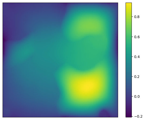
ECI-sampling – Solution

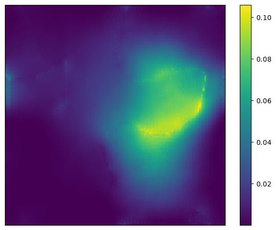
ECI-sampling – Data Error

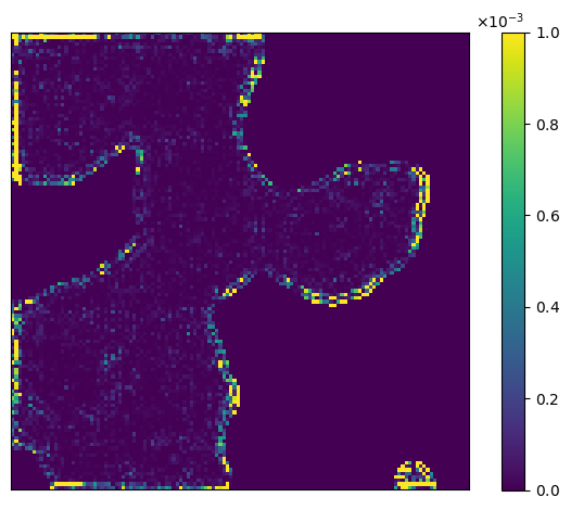
ECI-sampling – PDE Error

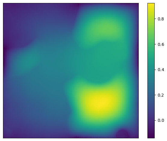
DiffusionPDE – Solution

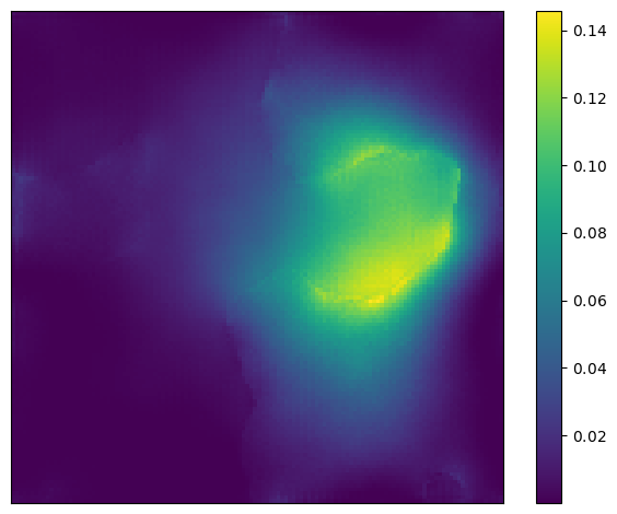
DiffusionPDE – Data Error

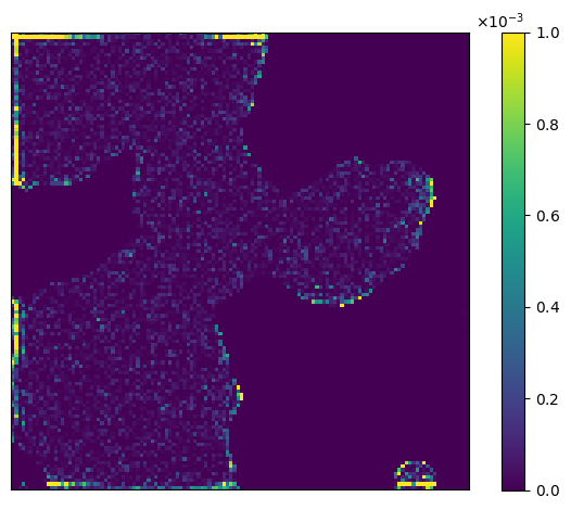
DiffusionPDE – PDE Error

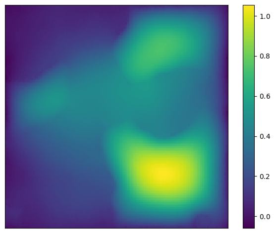
D-Flow – Solution

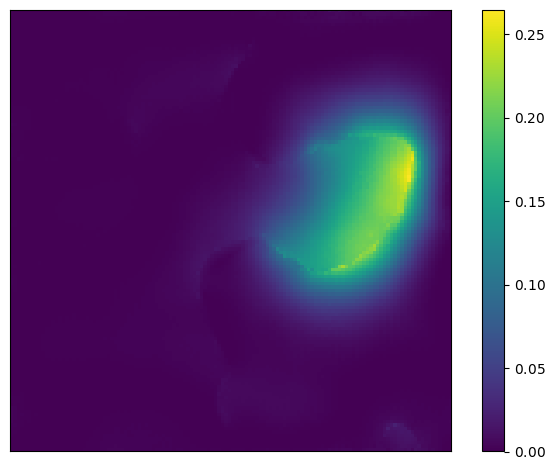
D-Flow – Data Error

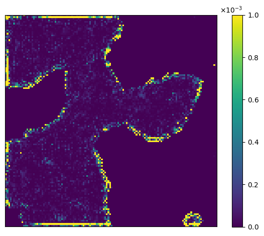
D-Flow – PDE Error

PIDDM – Solution

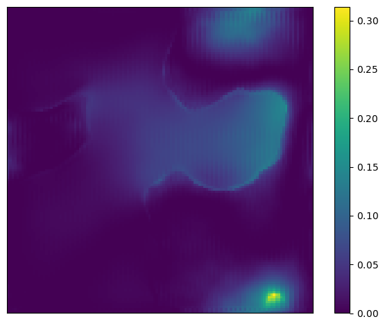
PIDDM – Data Error

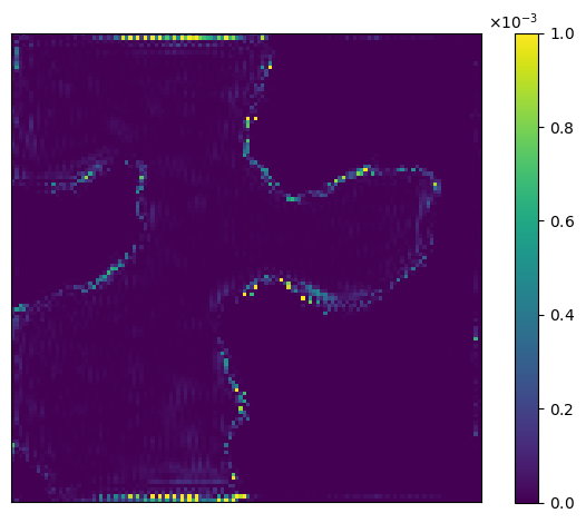
PIDDM – PDE Error

Figure 4: Qualitative comparison on the Darcy forward problem. Each column shows (left) the predicted solution field, (middle) point-wise data error, and (right) PDE residual error. Our PIDDM (bottom row) delivers visibly lower data and PDE errors than other baselines while maintaining sharp solution details.

Appendix F Additional Experiments

We investigate a controlled Mixture-of-Gaussians (MoG) setting to evaluate constraint satisfaction in generative models. The target distribution is a correlated, two-component Gaussian mixture:

$$p_{\mathrm{MoG}}(\mathbf{x})=\tfrac{1}{2},\mathcal{N}\left(\mathbf{x};[-1,-1]^{\top},\Sigma\right)+\tfrac{1}{2},\mathcal{N}\left(\mathbf{x};[+1,+1]^{\top},\Sigma\right),$$ (16)

where $\Sigma=\sigma^{2}\begin{bmatrix}1&\rho\ \rho&1\end{bmatrix},\sigma^{2}=0.04,\rho=0.99999.$ The high correlation $\rho=0.99999$ ensures that the analytic score function $\nabla_{\mathbf{x}}\log p_{\mathrm{MoG}}(\mathbf{x})$ remains well-defined, despite the near-singular covariance. The physical constraint is defined as:

$$\mathcal{F}({\bm{x}})=|{\bm{x}}_{0}-{\bm{x}}_{1}|^{2}=0.$$ (17)

Baselines. DPS and ECI both integrate the analytical score using 1000-step Euler discretization over $(0,1)$. DPS applies constraint guidance via gradient descent on $\mathcal{F}({\bm{x}})$ at each step, using a loss weight of $300$. ECI enforces the constraint by directly projecting the posterior mean to satisfy $\mathcal{F}({\bm{x}})=0$.

PIDDM. A teacher diffusion model is constructed using a probability-flow ODE with 100-step Euler integration, leveraging the analytic score. It generates 50,000 training pairs $(\bm{\varepsilon},{\bm{x}}_{0})$ which are used to train a one-step student model, a ReLU-activated MLP with two hidden layers (100 neurons each) via the loss:

$$\mathcal{L}_{\text{train}}=\frac{1}{N}\sum_{i=1}^{N}\left|d_{\bm{\theta}}(\bm{\varepsilon}_{i})-\bm{x}_{0,i}\right|^{2}+\lambda_{\text{train}}\mathcal{F}(d_{\bm{\theta}}(\bm{\varepsilon}_{i})),\quad\lambda_{\text{train}}=1.$$ (18)

Training uses Adam optimizer (lr = $10^{-3}$, batch size = 2048). During inference, latent noise $\bm{\varepsilon}$ is optimized via 80 steps of LBFGS with strong-Wolfe line search, learning rate $3\times 10^{-3}$, and gradient tolerance $10^{-7}$, with $\lambda_{\text{infer}}=1$.

Results. Figure 5(a) shows that all methods recover the bimodal structure of ${\bm{x}}_{1}$. However, as shown in Figure 5(b), DPS fails to fully satisfy the constraint, with ${\bm{x}}_{0}-{\bm{x}}_{1}$ spread over $\pm 10^{-2}$, while ECI enforces it exactly but distorts the marginal distribution. In contrast, PIDDM maintains both constraint satisfaction (standard deviation $\approx 2\times 10^{-3}$) and distributional fidelity.

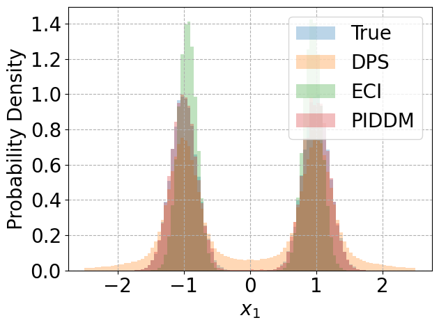
(a) Marginal distribution over $x_{1}$

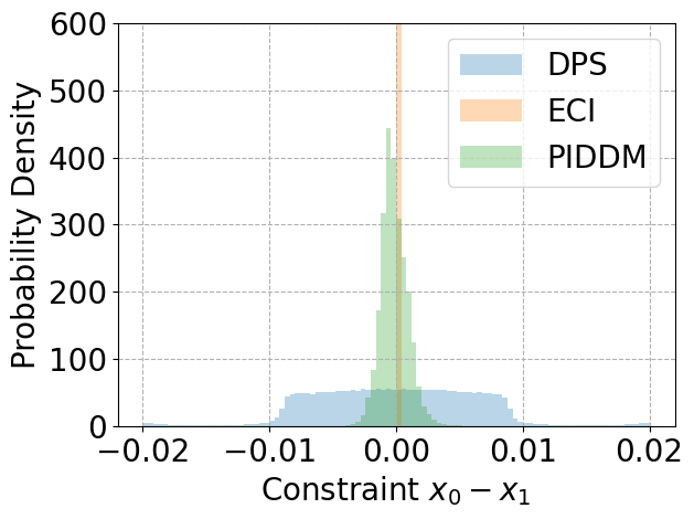
(b) Constraint deviation $x_{0}-x_{1}$

Figure 5: Constraint satisfaction on correlated MoG. Comparison of generated samples using DPS, ECI, and PIDDM. PIDDM closely matches the target distribution while satisfying constraints.

References

- (1) Martín Abadi, Paul Barham, Jianmin Chen, Zhifeng Chen, Andy Davis, Jeffrey Dean, Matthieu Devin, Sanjay Ghemawat, Geoffrey Irving, Michael Isard, et al. TensorFlow: a system for Large-Scale machine learning. In 12th USENIX symposium on operating systems design and implementation (OSDI 16), pages 265–283, 2016.
- (2) Brian DO Anderson. Reverse-time diffusion equation models. Stochastic Processes and their Applications, 12(3):313–326, 1982.
- (3) Jan-Hendrik Bastek, WaiChing Sun, and Dennis Kochmann. Physics-informed diffusion models. In The Thirteenth International Conference on Learning Representations, 2025.
- (4) Heli Ben-Hamu, Omri Puny, Itai Gat, Brian Karrer, Uriel Singer, and Yaron Lipman. D-flow: Differentiating through flows for controlled generation. arXiv preprint arXiv:2402.14017, 2024.
- (5) David Berthelot, Arnaud Autef, Jierui Lin, Dian Ang Yap, Shuangfei Zhai, Siyuan Hu, Daniel Zheng, Walter Talbott, and Eric Gu. Tract: Denoising diffusion models with transitive closure time-distillation. arXiv preprint arXiv:2303.04248, 2023.
- (6) Changgu Chen, Libing Yang, Xiaoyan Yang, Lianggangxu Chen, Gaoqi He, Changbo Wang, and Yang Li. Find: Fine-tuning initial noise distribution with policy optimization for diffusion models. In Proceedings of the 32nd ACM International Conference on Multimedia, pages 6735–6744, 2024.
- (7) Hao Chen, Yujin Han, Fangyi Chen, Xiang Li, Yidong Wang, Jindong Wang, Ze Wang, Zicheng Liu, Difan Zou, and Bhiksha Raj. Masked autoencoders are effective tokenizers for diffusion models. arXiv preprint arXiv:2502.03444, 2025.
- (8) Chaoran Cheng, Boran Han, Danielle C. Maddix, Abdul Fatir Ansari, Andrew Stuart, Michael W. Mahoney, and Bernie Wang. Gradient-free generation for hard-constrained systems. In The Thirteenth International Conference on Learning Representations, 2025.
- (9) Hyungjin Chung, Jeongsol Kim, Michael T Mccann, Marc L Klasky, and Jong Chul Ye. Diffusion posterior sampling for general noisy inverse problems. arXiv preprint arXiv:2209.14687, 2022.
- (10) John Crank. The Mathematics of Diffusion. Oxford University Press, 2 edition, 1975.
- (11) Peter A. Davidson. Turbulence: An Introduction for Scientists and Engineers. Oxford University Press, 2015.
- (12) Peter Dayan, Geoffrey E Hinton, Radford M Neal, and Richard S Zemel. The helmholtz machine. Neural computation, 7(5):889–904, 1995.
- (13) Bradley Efron. Tweedie’s formula and selection bias. Journal of the American Statistical Association, 106(496):1602–1614, 2011.
- (14) Patrick Esser, Sumith Kulal, Andreas Blattmann, Rahim Entezari, Jonas Müller, Harry Saini, Yam Levi, Dominik Lorenz, Axel Sauer, Frederic Boesel, et al. Scaling rectified flow transformers for high-resolution image synthesis. In Forty-first International Conference on Machine Learning, 2024.
- (15) Xiang Gao, Meera Sitharam, and Adrian E Roitberg. Bounds on the jensen gap, and implications for mean-concentrated distributions. arXiv preprint arXiv:1712.05267, 2017.
- (16) Xiefan Guo, Jinlin Liu, Miaomiao Cui, Jiankai Li, Hongyu Yang, and Di Huang. Initno: Boosting text-to-image diffusion models via initial noise optimization. In Proceedings of the IEEE/CVF Conference on Computer Vision and Pattern Recognition, pages 9380–9389, 2024.
- (17) Andi Han, Wei Huang, Yuan Cao, and Difan Zou. On the feature learning in diffusion models. arXiv preprint arXiv:2412.01021, 2024.
- (18) Yujin Han, Andi Han, Wei Huang, Chaochao Lu, and Difan Zou. Can diffusion models learn hidden inter-feature rules behind images? arXiv preprint arXiv:2502.04725, 2025.
- (19) Derek Hansen, Danielle C Maddix, Shima Alizadeh, Gaurav Gupta, and Michael W Mahoney. Learning physical models that can respect conservation laws. In International Conference on Machine Learning, pages 12469–12510. PMLR, 2023.
- (20) Geoffrey E Hinton and Ruslan R Salakhutdinov. Reducing the dimensionality of data with neural networks. science, 313(5786):504–507, 2006.
- (21) Jonathan Ho, Ajay Jain, and Pieter Abbeel. Denoising diffusion probabilistic models. Advances in neural information processing systems, 33:6840–6851, 2020.
- (22) Jonathan Ho and Tim Salimans. Classifier-free diffusion guidance, 2022.
- (23) Jiahe Huang, Guandao Yang, Zichen Wang, and Jeong Joon Park. DiffusionPDE: Generative PDE-solving under partial observation. In The Thirty-eighth Annual Conference on Neural Information Processing Systems, 2024.
- (24) Thomas JR Hughes. The finite element method: linear static and dynamic finite element analysis. Courier Corporation, 2003.
- (25) Frank P. Incropera, David P. DeWitt, Theodore L. Bergman, and Adrienne S. Lavine. Fundamentals of Heat and Mass Transfer. John Wiley & Sons, 7 edition, 2011.
- (26) John David Jackson. Classical Electrodynamics. John Wiley & Sons, 3 edition, 1998.
- (27) Christian Jacobsen, Yilin Zhuang, and Karthik Duraisamy. Cocogen: Physically-consistent and conditioned score-based generative models for forward and inverse problems, 2024.
- (28) Tero Karras, Miika Aittala, Timo Aila, and Samuli Laine. Elucidating the design space of diffusion-based generative models. Advances in neural information processing systems, 35:26565–26577, 2022.
- (29) Gavin Kerrigan, Giosue Migliorini, and Padhraic Smyth. Functional flow matching. arXiv preprint arXiv:2305.17209, 2023.
- (30) Diederik P Kingma and Jimmy Ba. Adam: A method for stochastic optimization. arXiv preprint arXiv:1412.6980, 2014.
- (31) Diederik P Kingma, Max Welling, et al. Auto-encoding variational bayes, 2013.
- (32) Randall J LeVeque. Finite difference methods for ordinary and partial differential equations: steady-state and time-dependent problems. SIAM, 2007.
- (33) Randall J LeVeque and Randall J Leveque. Numerical methods for conservation laws, volume 132. Springer, 1992.
- (34) Zongyi Li, Nikola Kovachki, Kamyar Azizzadenesheli, Burigede Liu, Kaushik Bhattacharya, Andrew Stuart, and Anima Anandkumar. Fourier neural operator for parametric partial differential equations. arXiv preprint arXiv:2010.08895, 2020.
- (35) Zongyi Li, Hongkai Zheng, Nikola Kovachki, David Jin, Haoxuan Chen, Burigede Liu, Kamyar Azizzadenesheli, and Anima Anandkumar. Physics-informed neural operator for learning partial differential equations. ACM/JMS Journal of Data Science, 1(3):1–27, 2024.
- (36) Yaron Lipman, Ricky T. Q. Chen, Heli Ben-Hamu, Maximilian Nickel, and Matthew Le. Flow matching for generative modeling. In The Eleventh International Conference on Learning Representations, 2023.
- (37) Xingchao Liu, Chengyue Gong, and qiang liu. Flow straight and fast: Learning to generate and transfer data with rectified flow. In The Eleventh International Conference on Learning Representations, 2023.
- (38) Xingchao Liu, Chengyue Gong, and qiang liu. Flow straight and fast: Learning to generate and transfer data with rectified flow. In The Eleventh International Conference on Learning Representations, 2023.
- (39) Xingchao Liu, Xiwen Zhang, Jianzhu Ma, Jian Peng, et al. Instaflow: One step is enough for high-quality diffusion-based text-to-image generation. In The Twelfth International Conference on Learning Representations, 2023.
- (40) Cheng Lu, Yuhao Zhou, Fan Bao, Jianfei Chen, Chongxuan Li, and Jun Zhu. Dpm-solver: A fast ode solver for diffusion probabilistic model sampling in around 10 steps. Advances in Neural Information Processing Systems, 35:5775–5787, 2022.
- (41) Cheng Lu, Yuhao Zhou, Fan Bao, Jianfei Chen, Chongxuan Li, and Jun Zhu. Dpm-solver++: Fast solver for guided sampling of diffusion probabilistic models. arXiv preprint arXiv:2211.01095, 2022.
- (42) Lu Lu, Pengzhan Jin, and George Em Karniadakis. Deeponet: Learning nonlinear operators for identifying differential equations based on the universal approximation theorem of operators. arXiv preprint arXiv:1910.03193, 2019.
- (43) Eric Luhman and Troy Luhman. Knowledge distillation in iterative generative models for improved sampling speed. arXiv preprint arXiv:2101.02388, 2021.
- (44) Jiafeng Mao, Xueting Wang, and Kiyoharu Aizawa. The lottery ticket hypothesis in denoising: Towards semantic-driven initialization. In European Conference on Computer Vision, pages 93–109. Springer, 2024.
- (45) Dimitra Maoutsa, Sebastian Reich, and Manfred Opper. Interacting particle solutions of fokker–planck equations through gradient–log–density estimation. Entropy, 22(8):802, 2020.
- (46) S Chandra Mouli, Danielle C Maddix, Shima Alizadeh, Gaurav Gupta, Andrew Stuart, Michael W Mahoney, and Yuyang Wang. Using uncertainty quantification to characterize and improve out-of-domain learning for pdes. arXiv preprint arXiv:2403.10642, 2024.
- (47) Alexander Quinn Nichol and Prafulla Dhariwal. Improved denoising diffusion probabilistic models. In International conference on machine learning, pages 8162–8171. PMLR, 2021.
- (48) A Paszke. Pytorch: An imperative style, high-performance deep learning library. arXiv preprint arXiv:1912.01703, 2019.
- (49) Maziar Raissi, Paris Perdikaris, and George E Karniadakis. Physics-informed neural networks: A deep learning framework for solving forward and inverse problems involving nonlinear partial differential equations. Journal of Computational physics, 378:686–707, 2019.
- (50) Danilo Jimenez Rezende, Shakir Mohamed, and Daan Wierstra. Stochastic backpropagation and approximate inference in deep generative models. In International conference on machine learning, pages 1278–1286. PMLR, 2014.
- (51) Robin Rombach, Andreas Blattmann, Dominik Lorenz, Patrick Esser, and Björn Ommer. High-resolution image synthesis with latent diffusion models. In Proceedings of the IEEE/CVF conference on computer vision and pattern recognition, pages 10684–10695, 2022.
- (52) Nadim Saad, Gaurav Gupta, Shima Alizadeh, and Danielle C Maddix. Guiding continuous operator learning through physics-based boundary constraints. arXiv preprint arXiv:2212.07477, 2022.
- (53) Andy Shih, Suneel Belkhale, Stefano Ermon, Dorsa Sadigh, and Nima Anari. Parallel sampling of diffusion models. Advances in Neural Information Processing Systems, 36, 2024.
- (54) Dule Shu, Zijie Li, and Amir Barati Farimani. A physics-informed diffusion model for high-fidelity flow field reconstruction. Journal of Computational Physics, 478:111972, 2023.
- (55) Gordon D Smith. Numerical solution of partial differential equations: finite difference methods. Oxford university press, 1985.
- (56) Jiaming Song, Chenlin Meng, and Stefano Ermon. Denoising diffusion implicit models. In International Conference on Learning Representations, 2021.
- (57) Yang Song, Prafulla Dhariwal, Mark Chen, and Ilya Sutskever. Consistency models, 2023.
- (58) Yang Song, Jascha Sohl-Dickstein, Diederik P Kingma, Abhishek Kumar, Stefano Ermon, and Ben Poole. Score-based generative modeling through stochastic differential equations. In International Conference on Learning Representations, 2020.
- (59) Stephen P. Timoshenko and James N. Goodier. Theory of Elasticity. McGraw-Hill, 3 edition, 1970.
- (60) Ashish Vaswani, Noam Shazeer, Niki Parmar, Jakob Uszkoreit, Llion Jones, Aidan N Gomez, Łukasz Kaiser, and Illia Polosukhin. Attention is all you need. Advances in neural information processing systems, 30, 2017.
- (61) Hao Wang, Weihua Chen, Chenming Li, Wenjian Huang, Jingkai Zhou, Fan Wang, and Jianguo Zhang. Noise re-sampling for high fidelity image generation, 2025.
- (62) Ruoyu Wang, Huayang Huang, Ye Zhu, Olga Russakovsky, and Yu Wu. The silent prompt: Initial noise as implicit guidance for goal-driven image generation. arXiv preprint arXiv:2412.05101, 2024.
- (63) Tianwei Yin, Michaël Gharbi, Richard Zhang, Eli Shechtman, Fredo Durand, William T Freeman, and Taesung Park. One-step diffusion with distribution matching distillation. In Proceedings of the IEEE/CVF conference on computer vision and pattern recognition, pages 6613–6623, 2024.
- (64) Sihyun Yu, Sangkyung Kwak, Huiwon Jang, Jongheon Jeong, Jonathan Huang, Jinwoo Shin, and Saining Xie. Representation alignment for generation: Training diffusion transformers is easier than you think. arXiv preprint arXiv:2410.06940, 2024.
- (65) Hongkai Zheng, Weili Nie, Arash Vahdat, Kamyar Azizzadenesheli, and Anima Anandkumar. Fast sampling of diffusion models via operator learning. In International conference on machine learning, pages 42390–42402. PMLR, 2023.
- (66) Zhenyu Zhou, Defang Chen, Can Wang, and Chun Chen. Fast ode-based sampling for diffusion models in around 5 steps. In Proceedings of the IEEE/CVF Conference on Computer Vision and Pattern Recognition, pages 7777–7786, 2024.
- (67) Zikai Zhou, Shitong Shao, Lichen Bai, Zhiqiang Xu, Bo Han, and Zeke Xie. Golden noise for diffusion models: A learning framework. arXiv preprint arXiv:2411.09502, 2024.