Calibrating Quantum Gates up to 52 Qubits in a Superconducting Processor
Abstract
Benchmarking large-scale quantum gates, typically involving multiple native two-qubit and single-qubit gates, is crucial in quantum computing. Global fidelity, encompassing information about inter-gate correlations, offers a comprehensive metric for evaluating and optimizing gate performance, unlike the fidelities of individual local native gates. In this work, utilizing the character-average benchmarking protocol implementable in a shallow circuit, we successfully benchmark gate fidelities up to 52 qubits. Notably, we achieved a fidelity of for a 44-qubit parallel CZ gate. Utilizing the global fidelity of the parallel CZ gate, we explore the correlations among local CZ gates by introducing an inter-gate correlation metric, enabling one to simultaneously quantify crosstalk error when benchmarking gate fidelity. Finally, we apply our methods in gate optimization. By leveraging global fidelity for optimization, we enhance the fidelity of a 6-qubit parallel CZ gate from 87.65% to 92.04% and decrease the gate correlation from 3.53% to 3.22%, compared to local gate fidelity-based optimization. The experimental results align well with our established composite noise model, incorporating depolarizing and -coupling noises, and provide valuable insight into further study and mitigation of correlated noise.
I Introduction
Realistic quantum computers suffer from noise, hindering themselves from demonstrating an advantage over their classical counterpart [1, 2, 3, 4, 5]. Quantum error correction is the key to reducing noise [6, 7, 8, 9, 10], yet its implementation hinges on the availability of high-fidelity quantum gates and weak correlations among different gate operations [11, 12, 13]. Thus, diagnosing the noise level and assessing the interaction within the quantum circuits is essential to improving their performance and, hence, realizing fault-tolerant quantum computing. Within a step of quantum circuits, single-qubit and two-qubit gates are parallelly implemented to reduce the circuit depth. Due to the potential crosstalk and residual coupling between the qubits [14], the local gate fidelities may be insufficient to give an overall evaluation of the global gate. In contrast, global gate fidelity contains information about correlations among different local gates, providing an overall performance metric.
As quantum hardware advances and platforms grow, large-scale quantum gate calibration becomes increasingly crucial. Researchers have made great efforts to develop practical benchmarking methods [15, 16, 17] and enlarge the gate calibration size. Currently, the most frequently used method to evaluate the quantum gate fidelity is randomized benchmarking (RB) [18, 19, 20, 21, 22], which enjoys the advantage of low complexity and robustness to state preparation and measurement errors. Nonetheless, the original RB protocol [20] is only realized up to three qubits [23] owing to the compiling problem of global Clifford gates. Several RB variants [24, 25, 26] were proposed circumventing compiling issues and significantly advanced the benchmarking size to 10 qubits for an individual gate via cycle benchmarking [25] and 27 qubits for a gate set via mirror RB [26].
Nonetheless, a gap exists between these achievements and the scale of state-of-the-art quantum computers. Currently, quantum computers have been realized with tens of or even hundreds of qubits in superconducting [ZHU2022advantage, 28, 29], ion trap [30, 31], and neutral atom systems [32]. Calibrating larger gates is demanding for assessing and enhancing the performance of current quantum computers. Meanwhile, a noticeable challenge to achieving this goal is the low fidelity often associated with large-scale gates. Many RB protocols require repeated execution of the target gate. However, noise can prevent the gate from being repeated without significant signal loss, which can render the protocol ineffective. Resolving this issue requires enhancing benchmarking protocols to ensure their effectiveness in short-depth circuits and achieving the realization of higher-performance quantum gates.
In this work, to achieve large-scale gate calibration, we utilize the character-average benchmarking (CAB) [33] protocol. This method can evaluate the fidelity robust to state preparation and measurement errors for an individual Clifford gate up to a local unitary transformation and be scalable with respect to the system size. Compared to cycle benchmarking [25] that also aims to evaluate the individual gate fidelity, CAB requires shorter circuit depth and can tolerate higher gate errors and benchmarking larger gates. Additionally, CAB exhibits smaller statistical fluctuations than cycle benchmarking, with more details shown in the Supplemental Material [38]. Meanwhile, in experiments, we improve gate fidelity and reduce a significant portion of gate control errors via qubit frequency adjustment and pre-calibration of gate parameters, as elaborated in Methods. The high fidelity and nearly depolarizing noise of the quantum gates are crucial to our success in realizing large-scale CAB experiments.
Here, we consider two important types of gates for experimental benchmarking. One is a fully connected gate composed of two layers of CZ gates and two layers of local Clifford gates. This gate is a part of the brickwise architecture circuit with an efficient realization scheme on current devices and hence is favored in variational quantum algorithms [34]. It also plays an essential role in other quantum information processing tasks like simulating a nearest-neighbor interacting Hamiltonian evolution. We benchmark such gates up to 46 qubits and get a fidelity of dressed with local twirling gates.
We also benchmark the parallel CZ gate, composed of parallelly implemented local CZ gates, which excels in generating entanglement across multiple parties and is essential in preparing graph states and executing numerous quantum algorithms [35, 36]. We benchmark such gates from 4 to 44 qubits. The average fidelity of a single local CZ gate is about and does not decrease with the qubit number increase.
With the global fidelity of the parallel CZ gate, we characterize the correlation among the local CZ gates. This procedure can be done simultaneously when benchmarking global fidelity without extra experiments. The correlation data provides the interaction information within the circuit and helps to evaluate and optimize the gate performance. The correlation of the 44-qubit parallel CZ gate turns out to be weak and constantly positive. In contrast, the results of the 52-qubit parallel CZ gate present some negative values. The experimental results are well explained by our established composite noise model, which incorporates local depolarizing and -coupling noises. The correlation magnitude positively depends on the coupling strength. Interestingly, the correlation sign between two gates varies in two cases: staying positive in two-gate coupling yet turning negative in three-gate coupling when one gate strongly couples with a third one. The correlation results help identify coupling gates and advance the study of correlated noise.
Since an important application of fidelity benchmarking is gate optimization, we demonstrate optimization experiments for parallel CZ gates and compare outcomes when setting the target function as the parallel CZ gate fidelity and the individual local CZ gate fidelities. We observe better results of the former. This result validates the effectiveness of CAB and suggests that global fidelity is more effective in optimizing quantum circuit performance, originating from containing more correlation information. The optimization result is consistent with the -coupling noise model. When three gates couple, improving the fidelity of one local CZ gate may reduce the fidelities of others. This antagonistic relationship demonstrates the limitations of local fidelities.
II Results
II.1 Preliminary
Let us start with briefly revisiting the concept of gate fidelity. Any noisy quantum gate can be treated as a composite of its noise channel , and the ideal gate , expressed as . In this work, the fidelity of gate refers to the process fidelity of , defined by,
| (1) |
where is the number of qubits, and represents the -qubit Pauli group. This process fidelity is a linear function of the average fidelity, a metric commonly employed in quantum gate benchmarking studies. The summation in Eq. (1), initially spanning terms, can be effectively restructured into terms as follows:
| (2) |
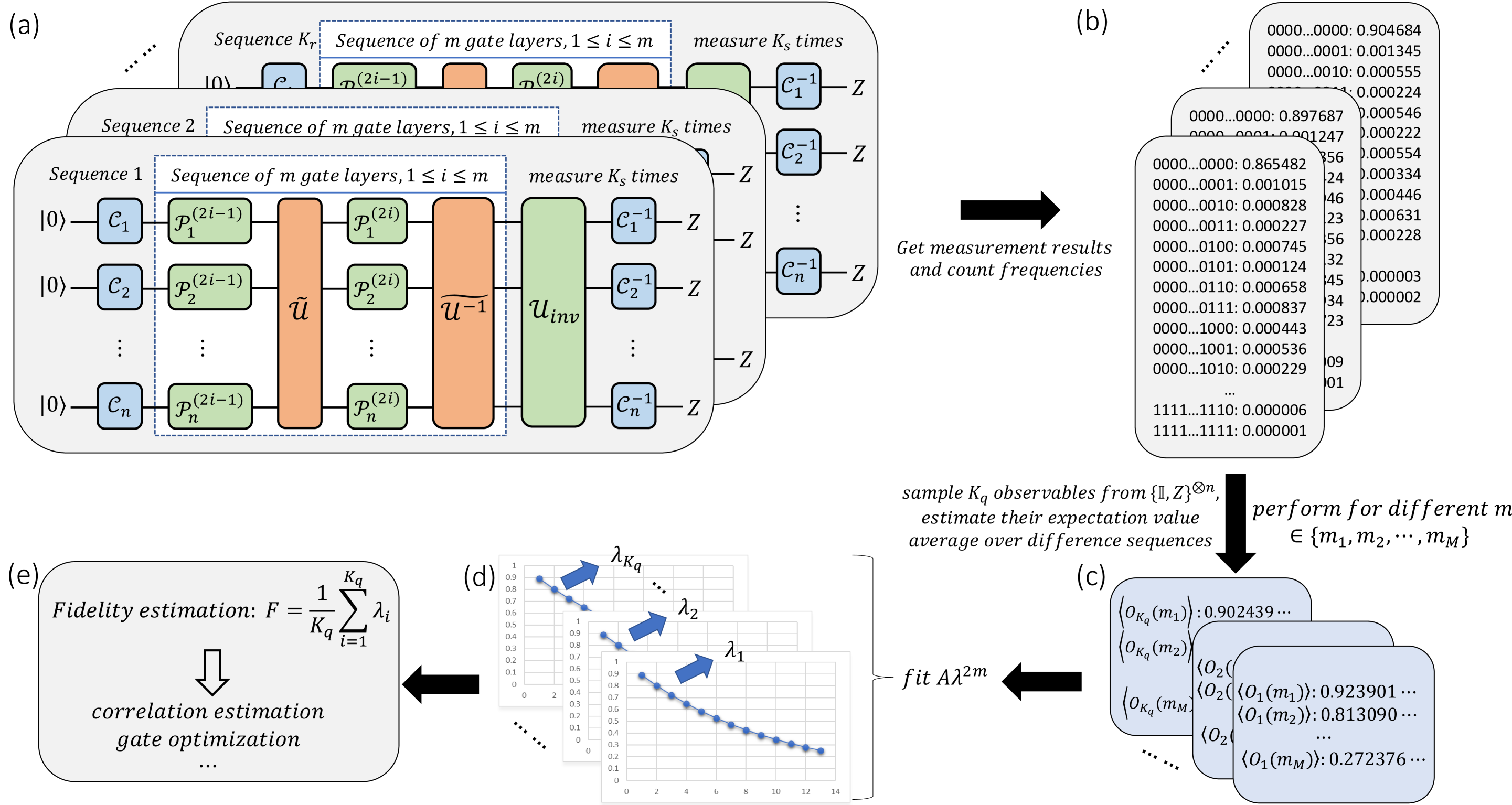
where denotes a bitstring that takes 0 on bit if acts as the identity on qubit and takes 1 if acts non-trivially, and signifies the weight of the bitstring . The quantity is termed the weighted quality parameter of with weight , and below, we concisely refer to it as the quality parameter of .
The core of CAB lies in assessing the quality parameter of the channel through the circuit depicted in Figure 1(a), with and being the Pauli-twirled noise channels of and , respectively. This approach yields the CAB fidelity of , closely approximating ’s fidelity under physically reasonable conditions [33]. Hereafter, we refer to the CAB fidelity simply as the gate fidelity unless stated otherwise. While estimating all quality parameters for fidelity evaluation demands exponential resources, the number of quality parameters necessary for accurate fidelity estimation within acceptable error margins and confidence levels is independent of the qubit count, thereby ensuring the scalability of the protocol. The whole procedure is shown in Figure 1 and elaborated in Methods. Note that the fidelity evaluated by this procedure is associated with the noise of and that of the local twirling gates adjacent to and , referred to as dressed fidelity. To isolate ’s fidelity, one can employ interleaved RB techniques [22], comparing the dressed fidelity against the local twirling gate fidelity. Particularly, the fidelity of is derived by [22]
| (3) |
with and the dressed and twirling gate fidelities, respectively. The local twirling gate fidelity itself is determined through CAB, with the identity operation as the target gate.
II.2 Fully connected gate and parallel CZ gate benchmarking
Our CAB experiments for the fully connected gate and the parallel CZ gate are conducted on a 54-qubit superconducting quantum computer. On a two-qubit system, the CZ gate is , and its parallel extension across multiple qubits is defined by , where denotes the CZ gate acting on a specific qubit pair, , making a -qubit gate. The fully connected gate comprises two layers of different parallel CZ gates intertwined with two layers of single-qubit gates, as shown in Figure 2(a). One of the parallel CZ gates connects qubits 1 and 2, 3 and 4, … and the other connects qubits 2 and 3, 4 and 5…
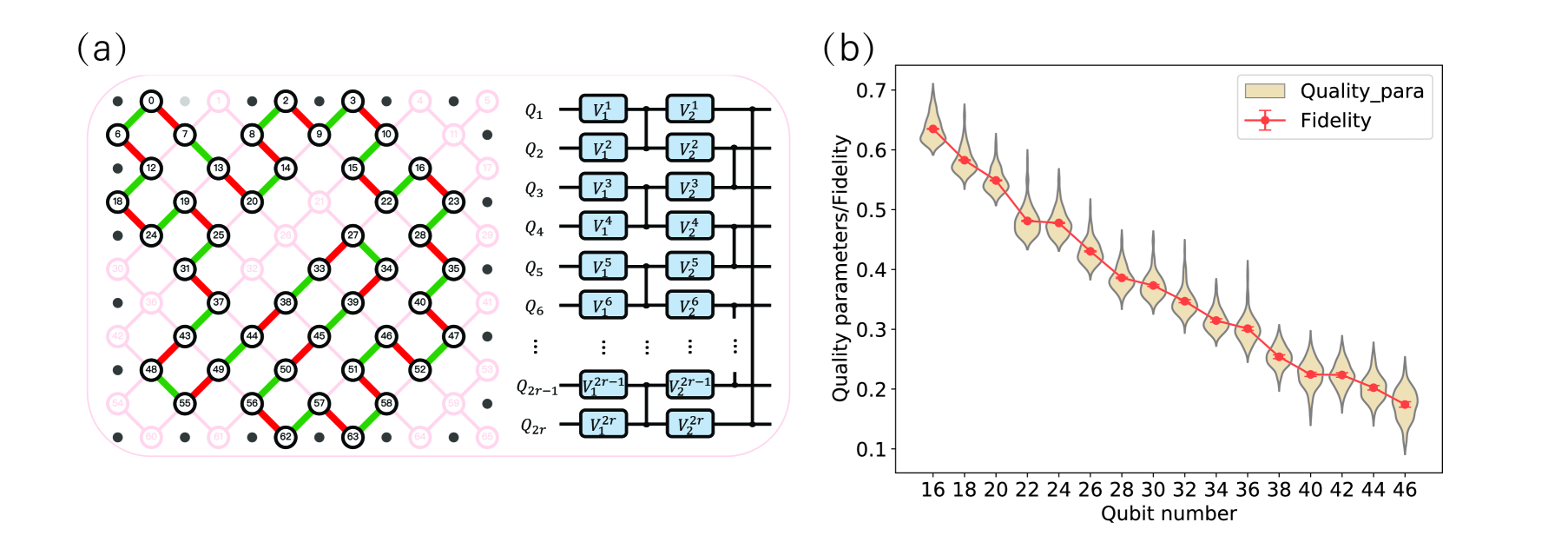
Fully connected gate benchmarking.—The single-qubit gates in the fully connected gate, like and in Figure 2(a), are free to vary. In quantum information tasks like variational quantum algorithms, they are normally chosen according to specific problems. In our experiments, we randomly sample all the single-qubit gates from the Clifford group so that the global gate is a Clifford gate and can be benchmarked with CAB. It is worth mentioning that cycle benchmarking requires repeatedly implementing the target gate proportional to the gate order, defined as the smallest positive integer to make . The fully connected gate generally has a rapidly increasing order with respect to the qubit number, and the order has already been thousands on average for 16 qubits, which we show in the Supplemental Material [38]. The long-depth circuit will lead to extremely noisy experimental results and cannot provide effective benchmarking. Instead, by using the target gate and its inverse, this gate can be benchmarked within a short-depth circuit using CAB.
We realized the fully connected gate with qubit numbers from 16 to 46 and benchmarked its dressed fidelity. The dressed fidelity of each target gate is estimated with circuit depths of through 50 circuit samples per circuit depth and performed 20,000 measurements per circuit. Theoretically, larger circuit depth differences can reduce fidelity estimation fluctuations, but practical constraints limit how deep the circuits can be. To reduce the impact of gate noise on the measurement results, we choose the circuit depths below 2.
Based on the measurement results, we estimated 100 quality parameters and averaged them to compute the gate fidelity. The results are shown in Figure 2(b), ranging from to for qubit numbers from 16 to 46, with the full data available in the Supplemental Material [38]. The quality parameters are distributed near the mean value, meaning the noise is close to a depolarizing noise. This feature is extremely useful in realizing CAB experiments in a low-fidelity region. If the noise is far from the depolarizing noise, like the unitary noise, and the fidelity is low, the quality parameters may be below 0. Since a quality parameter is obtained by fitting it to as shown in Figure 1, a negative quality parameter is indistinguishable from and cannot be obtained correctly by the exponential fitting.
Parallel CZ gate benchmarking.—The benchmarking for the parallel CZ gates contains two patterns, depicted in Figure 3(a) using two distinct colors. We first evaluate the fidelities of the gates within the orange pattern, consisting of 22 pairs of CZ gates aligned in the same physical direction. This benchmarking was conducted progressively, starting with 2 pairs of CZ gates and incrementally including more gates up to the full set of 22 pairs. Subsequently, we evaluate the gate correlations within the orange and the blue patterns. The latter incorporates 26 pairs of CZ gates and engages almost the entire quantum processor.
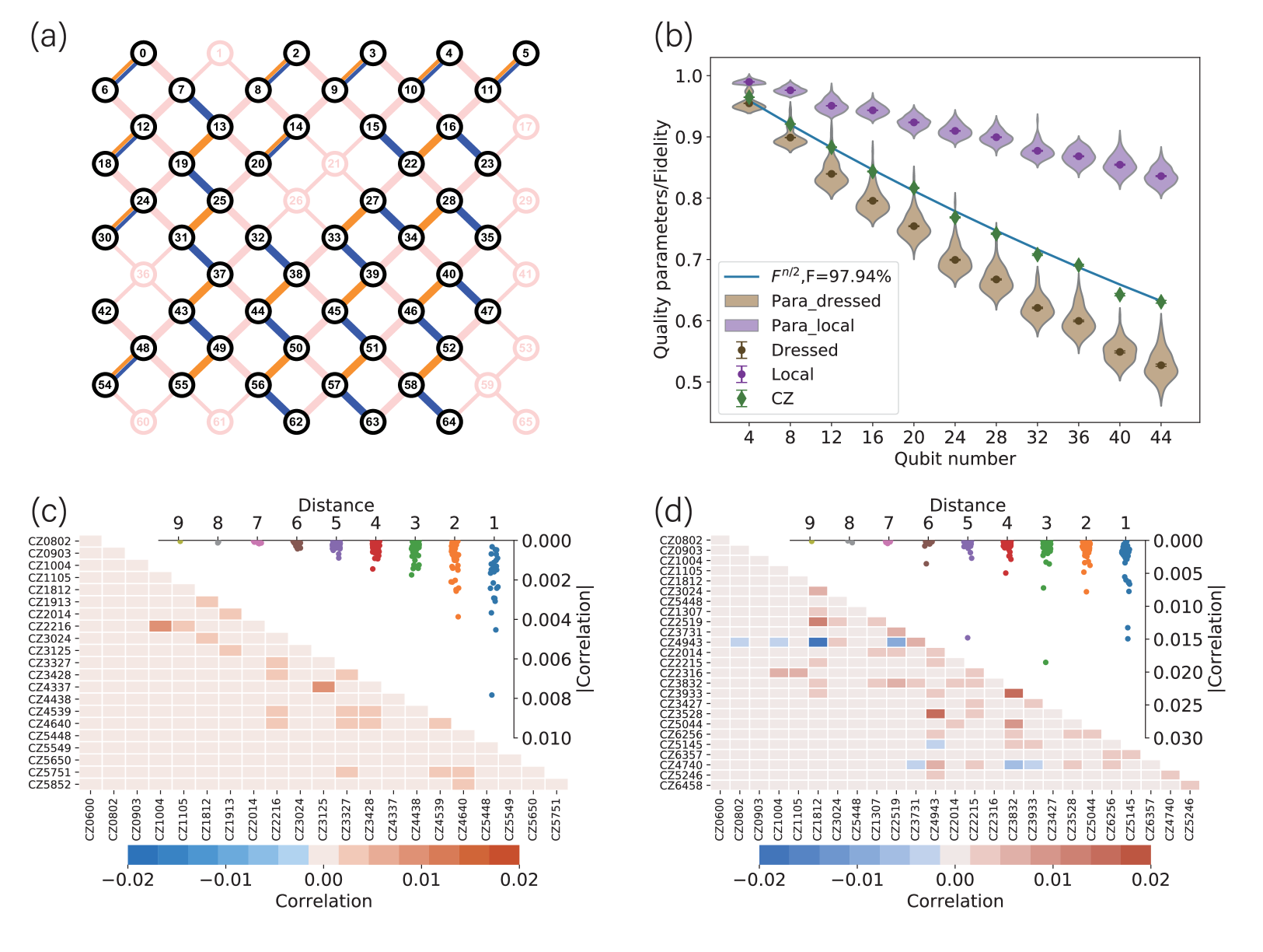
The settings for benchmarking parallel CZ gates within the orange pattern are the same as that for the fully connected gate, except the circuit depths changed to . In this experiment, we benchmark both the dressed fidelity and the local twirling gate fidelity. The local twirling gate fidelity is obtained by changing the target gate with the identity operation. We then use the interleaved technique [22] and Eq. (3) to isolate the pure parallel CZ gate fidelity.
In Figure 3(b), we show the noise channel quality parameter distribution for the dressed parallel CZ gates and the local gates with violin plots. The mean value equals the fidelity and is shown with a point. The green diamond-shaped points represent the pure fidelities of the parallel CZ gates within the orange pattern. The largest one, or the 22-pair parallel CZ gate, possesses a fidelity of . These fidelities have been fit using the function , where is the qubit number. The fit aligns closely with our experimental data, suggesting a fidelity value of approximately for a single CZ gate. This indicates that, in the orange pattern, the fidelity of individual CZ gates remains nearly constant and is not affected by an increase in qubit number. This observation implies that the crosstalk among these parallel CZ gates is either limited to short-range interactions or is remarkably minimal. Such a characteristic is critical for the implementation of quantum error correction. The detailed fidelity and standard error data are available in the Supplemental Material [38].
II.3 Correlation benchmarking
Beyond gate fidelity, our analysis extends to examining correlations within parallel CZ gates. We define this correlation as the deviation of the parallel CZ gate fidelity from the product of the fidelities of its comprising local CZ gates. The concept of correlation is elaborated in Methods. Any nonzero correlation value emerges as an indicator of interactions among the local gates.
The correlations among every two CZ gates within the orange and blue patterns are visualized through heatmaps in Figures 3(c) and (d), respectively. Additionally, we plot the correlation magnitudes as a function of the physical distance between CZ gates in the processor. For the orange pattern, we used the pure CZ gate fidelities from the parallel CZ gate benchmarking experiment to evaluate the correlation. The result of the blue pattern is obtained by another experiment. The orange pattern exhibits a notable feature: correlations between CZ gates are consistently positive and pronounced only when the gates are close. This observation suggests a negligible presence of long-range interactions in the implementation. However, the 26-pair parallel CZ gate within the blue pattern reveals different performance, with substantially higher correlations even for distant CZ gates, indicating the existence of long-range interactions within this configuration. The difference between the two patterns can be explained by whether a parallel calibration of CZ gates before benchmarking exists. Before experiments, gates in the same direction–such as all the two-qubit gates in the orange pattern–were calibrated in parallel using the method detailed in the “Parallel calibration of controlled-Z gate parameters with back probability” subsection in Methods. To maximize the qubit number of a pattern, the blue pattern is formed by combining gates in two directions. The results show that correlation benchmarking serves as an additional indicator of gate performance, alongside fidelity.
In Methods, we establish a noise model composed of depolarizing and -coupling noises to explain the correlation benchmarking results. The model first introduces a local depolarizing noise on each gate, followed by a unitary correlated noise. The Hamiltonian of the correlated noise is a summation of pairwise on each pair of CZ gates, where the coefficients depend on the coupling strengths. Our analysis focuses on the two-gate and three-gate coupling cases. A natural result is that the correlation value between two gates positively depends on their own coupling strength. Weak correlation implies weak coupling. Interestingly, we find that when only two gates couple with each other, the correlation is always positive. The correlation value is normally less than 0.001 for uncorrelated gates and can be on the order of 0.01 for correlated gates, which is consistent with the experimental data. Nonetheless, if one of the two gates couples with a third gate, the correlation between the original two gates can become negative. Particularly, when one gate is strongly coupled with the third gate, and the other gate is weakly coupled to it, the negative correlation becomes significant.
Applying the theoretical analysis to the experimental data, we observe that most correlation values are positive, corresponding to weak coupling or two-gate coupling cases. The results of the orange pattern can be fully explained by two-gate coupling. The pair of CZ2216 and CZ1004 and the pair of CZ4337 and CZ3125 exhibit the strongest couplings. The CZ gates in the two pairs are both nearest neighbors. For the blue pattern, negative correlation values are observed, indicating that the two-gate coupling model is not sufficient to explain the data. Take the pair of CZ4943 and CZ1812 as an example, the negative correlation value implies that besides the coupling between CZ4943 and CZ1812, there exists a third gate strongly coupled with CZ4943 or CZ1812. From the correlation data, we infer that a neighbor of CZ4943, like CZ3731, couples strongly with CZ4943 but not with CZ1812. The coupling relationship among these three CZ gates can lead to a negative correlation between CZ4943 and CZ1812. Note that in real experiments, couplings can involve more than three gates, making the origins of negative correlations more complicated than the three-gate model described here. We expect our results to inspire more explorations into the correlation and coupling among quantum gates.
II.4 Parallel CZ gate optimization
In addition to benchmarking, we conducted optimization on parallel CZ gates, employing two distinct approaches: optimizing with global fidelity and optimizing with individual local CZ gate fidelities. In both cases, the Nelder-Mead algorithm is utilized for optimization [37, 39]. Note that the noise of the target gate is much larger than that of the local twirling gates, and the fidelities of the local twirling gates are stable. The noise of the target gate dominates the dressed fidelity, making this quantity sufficient for optimization. To reduce benchmarking time, we optimize using the dressed fidelity, avoiding additional benchmarking of local twirling gates and the interleaved procedure. To minimize the influence of other unstable factors on gate fidelity, we measure both the fidelity of the parameters being iterated (iterative fidelity) and the fidelity of the initial parameters as a reference (reference fidelity) throughout the optimization process. The optimization target function is defined as the difference between these two fidelities. Before this optimization experiment, each local CZ gate was calibrated with the “fast calibration” and “parallel calibration” approaches shown in Methods.
In our experiments, the parallel CZ gate comprises optimizable parameters with the qubit number. We chose as 4 and 6 so that the number of parameters is suitable for the Nelder-Mead algorithm to work. Optimizing gates with tens of qubits requires more scalable optimization algorithms. Figure 4 presents the optimization results for a parallel CZ gate comprising 3 local CZ gates on 6 qubits. The topology of the three CZ gates and the optimization procedure are shown in Figure 4(a). The three gates are relatively close, which are more likely to correlate with each other. Meanwhile, the readout channels of these three gates are relatively stable compared to other gates, ensuring minimal influence of environmental noise on the optimization procedure.
The progression of fidelities during the optimization is depicted in Figure 4(b), and the inter-gate correlations, calculated based on data from iterations 100-180, are illustrated in Figure 4(c). This specific iteration range is chosen as it is the phase of the iterative parameter convergence and stable reference fidelities, indicating a reduced impact from other fluctuating factors. Further experimental details and results of a 4-qubit setup are available in the Supplemental Material [38].
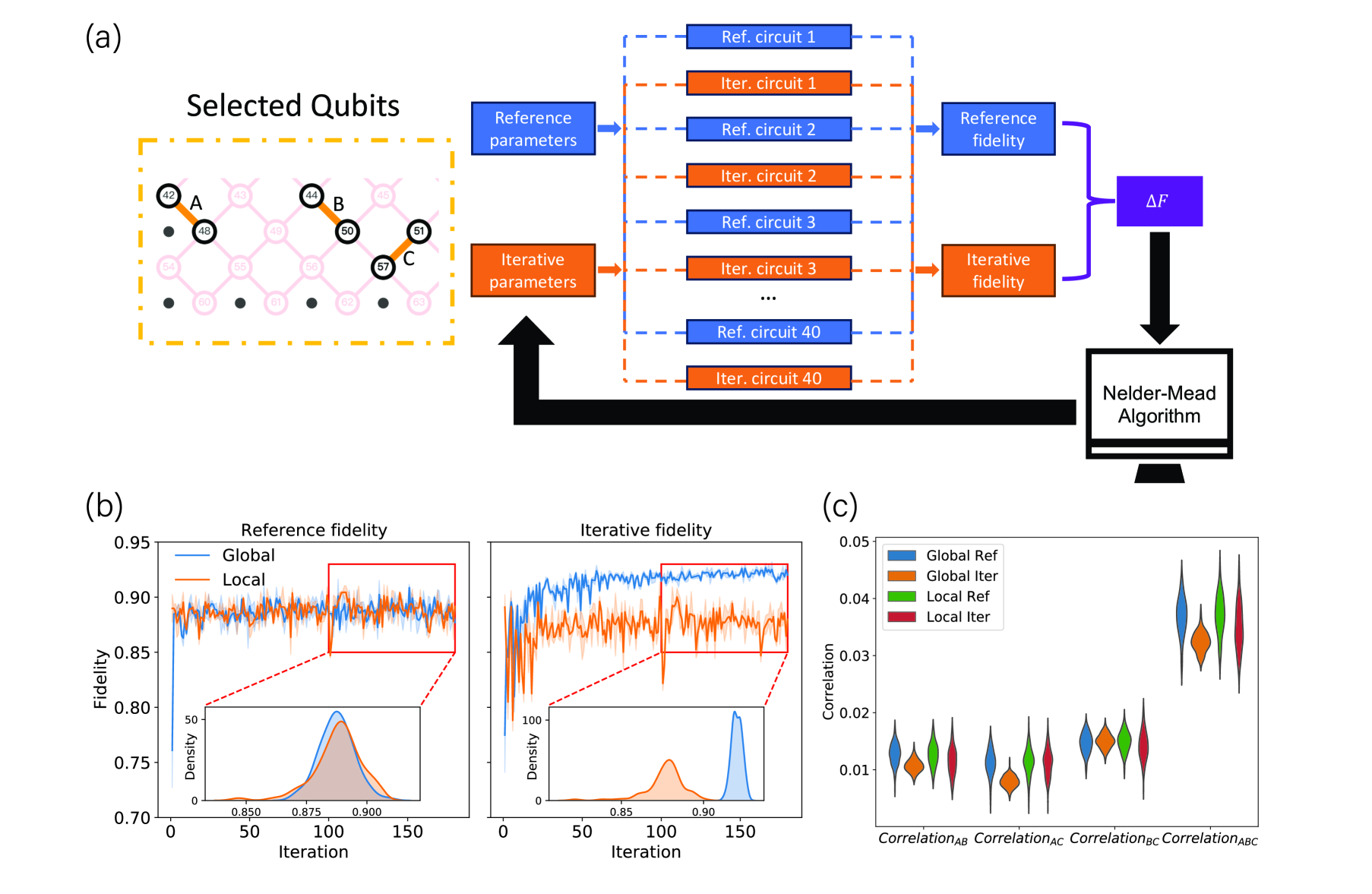
Below, we compare the optimization results employing global fidelity and the local gate fidelities with data from iterations 100-180. The fidelity is improved to 92.04% and 87.65%, and the correlation is reduced to 3.22% and 3.53% when using global fidelity and the local gate fidelities for optimization, respectively. It is clear that using global fidelity for optimization more effectively enhances fidelity and reduces correlation. Using local gate fidelities tends to yield inferior optimization outcomes, attributable to the lack of correlation information within the target function. In Methods, we use the -coupling model to explain the difference between global and local gate fidelities. When three gates are mutually coupled, optimizing one local fidelity may cause a decrease in the other two. This antagonistic relationship between local fidelities can trap the optimization in a local region. In contrast, global fidelity incorporates all correlation information, allowing the optimization to proceed monotonically. This finding underscores the significance of correlation in optimizing parallel gates and demonstrates the crucial advantage and essence of benchmarking large-scale quantum gates.
III Discussion
In conclusion, we utilize CAB to conduct large-scale experiments of benchmarking the fully connected and parallel CZ gates. The benchmarking of gate correlation provides quantity to evaluate the quantum gate performance beyond gate fidelity, allowing the detection of long-range interaction, which may further be useful in studying many-body physics. Combined with the -coupling noise model, it is feasible to detect the coupling pattern of the parallel gates with correlation benchmarking. The established noise model also provides insight into further study of near-term quantum devices and quantum error correction.
The results highlight the crucial role of correlation in optimizing parallel quantum gates. Practically, one can decompose the circuit into multiple layers and optimize each layer with improved gate fidelity and reduced inter-gate correlation. This approach is more effective than optimizing each local gate individually, as evidenced by our optimization results. Meanwhile, one can first identify strongly coupled gates through correlation benchmarking and divide them into distinct groups. Gates within each group are strongly correlated, while groups themselves are weakly correlated. By optimizing each group individually, the overall performance of the entire layer can be enhanced. This approach simplifies the optimization process by focusing on the dominant gate correlations.
Our experimental methodology for benchmarking and optimizing large-scale gates applies to enhancing all Clifford circuits up to a local gauge transformation [33], including the essential case of quantum error-correcting code circuits [40]. Typical quantum encoding schemes like surface codes [9, 10] or, more generally, quantum low-density-parity-check codes [41], involve tens or even hundreds of qubits. Optimizing such large batches involves managing many gate parameters, necessitating the development of scalable optimization algorithms rather than solely scalable benchmarking. In the future, advanced large-scale optimization algorithms, particularly gradient-free ones, will help to explore large-gate optimization, ultimately contributing to realizing universal fault-tolerant quantum computers.
Acknowledgements.
We thank Pengyu Liu, Yuxuan Yan, and Zhiyuan Chen for the helpful discussions. This work was supported by the Innovation Program for Quantum Science and Technology (Grant No. 2021ZD0300200), Anhui Initiative in Quantum Information Technologies, Special funds from Jinan Science and Technology Bureau and Jinan high tech Zone Management Committee, Shanghai Municipal Science and Technology Major Project (Grant No. 2019SHZDZX01), the New Cornerstone Science Foundation through the XPLORER PRIZE, the Key-Area Research and Development Program of Guangdong Province (Grant No. 2020B0303060001), Shanghai Science and Technology Development Funds (Grant No. 23YF1452500), the National Natural Science Foundation of China (Grant No. 12174216), the Innovation Program for Quantum Science and Technology (Grant No. 2021ZD0300804).IV Methods
IV.1 Procedure of character-average benchmarking
Below in Box IV.1, we introduce the procedure of the CAB protocol when benchmarking an -qubit Clifford gate corresponding to Figure 1. For target gates as non-Clifford gates and more protocol details, one can refer to Ref. [33].
Note that the procedure in Box IV.1 differs from the original one in Ref. [33]. The main modification lies in step 5. In Ref. [33], one does not sample observables but take all observables from , which requires . Here, we only need to set to ensure that Eq. (4) only differs from the fidelity estimated by traversing observables a small quantity, , with a high confidence level, . This can be seen from Hoeffding’s inequality, which is shown below. Note that is limited in the region .
| (5) |
Setting , we get . Note that is irrelevant to the qubit number . Thus, the complexity of the classical postprocessing is independent of . The number of sampled sequences for fidelity estimation is also independent of as proved in Ref. [33]. Thus, the whole benchmarking protocol is scalable.
IV.2 Correlation
Here, we introduce the formal definition of the correlation of a parallel gate. We consider a parallel gate, , where is more local or acts on fewer qubits than . Normally, is a one-local or two-local gate in experiments. That is, only acts on one qubit or two qubits. Via CAB, one can simultaneously get the fidelity of and the fidelities of , denoted as and , respectively. If there is no correlation among , the noise channel of can be expressed as where is the individual noise of . Then, the global fidelity, , would be equal to the product of local gate fidelities, . In reality, the interaction among different gates would make the two values different. We define the following quantity to characterize the total correlation among ,
| (6) |
The denominator is a normalization factor. When the correlation is positive, the global fidelity is larger than the product fidelity, indicating that the correlation helps to increase the global fidelity. Since Eq. (6) is defined among gates, we call it -correlation. Except for -correlation, one can also obtain -correlation among each gates in where for parallel gate . Note that since and can be obtained simultaneously from the same experimental data, gate correlation can also be evaluated concurrently without any additional experimental effort.
IV.3 Experimental platform
In this work, we utilized a processor with the same design as the processor [42], and selected up to 54 qubits for our experiments. The basic performance of the processor is shown in Table 1, where the single-qubit gate error and the two-qubit CZ gate error with a median of and by cross-entropy benchmarking (XEB) [43, 44, 45]. Our scheme to realize a two-qubit CZ gate is implementing an all-microwave coupler with a fixed gate time of 110 ns [46]. The approach involves applying a microwave signal with an envelope and a driving frequency of to the tunable coupler, with an extra flux given by . When the driving frequency matches the energy difference between the and states, i.e., , resonance takes place between these two states. Here, is a computational-basis state with each qubit at state , and is a state outside the computational subspace. However, due to the nonlinear relationship between the extra flux and the coupling strength, although is a good single-frequency signal when transformed into the coupling strength, the signal contains significant frequency components not only at , but also at and . Therefore, when considering the frequency layout of qubits, it is necessary to avoid , , and equal to either or .
| Parameters | Mean | Median | SD |
| Qubit maximum frequency (GHz) | 5.504 | 5.504 | 0.093 |
| Qubit idle frequency (GHz) | 5.411 | 5.403 | 0.104 |
| Qubit anharmonicity (MHz) | -243 | -242 | 4 |
| at idle frequency (s) | 22.14 | 22.11 | 7.60 |
| at idle frequency (s) | 4.94 | 4.55 | 3.24 |
| Readout () | 1.03 | 0.90 | 0.72 |
| Readout () | 3.82 | 3.43 | 1.64 |
| 1Q XEB () | 0.31 | 0.24 | 0.18 |
| 2Q-CZ XEB () | 3.35 | 3.21 | 0.98 |
Before our experiments, we adjusted the qubit frequency and calibrated the parameters for each local gate to make the processor perform well. In the following subsections, we will elaborate on this procedure in detail.
IV.4 Frequency conflict and frequency adjustment
The distribution of qubit frequencies is typically constrained within a range of 0-400 MHz due to magnetic flux noise and the bandwidth of the digital-to-analog converter. When arranging the qubit frequencies, the following factors need to be considered and balanced: (1) Energy relaxation time and dephasing time . (2) Spacing of frequencies between neighboring qubits and next-to-nearest neighboring qubits. (3) Two-qubit gate frequencies, as well as their second and fourth harmonic frequencies, and the frequency conflicts with and . (4) Maximum frequencies for each qubit, which represent the available frequency range for each qubit. By defining the above factors as error functions and frequency domains, we can obtain a set of theoretically optimal frequencies. After adjusting the frequencies of all qubits to the optimized arrangement, a majority of single-qubit gates and two-qubit gates can achieve high fidelity through standard calibration. However, local fine-tuning is still required for poorly performing gates. Additionally, the performance of a quantum processor may deteriorate during certain time intervals due to long-term periodic frequency variations in two-level systems. This also requires fine-tuning of the corresponding qubits. Qubit frequency tuning is relatively frequent and tedious, as adjusting the frequency of one qubit requires re-calibrating two-qubit gates associated with it. Therefore, it is crucial to calibrate single-qubit gates and two-qubit gates efficiently in this process. On the other side, the success of subsequent benchmarking relies on an initial good adjustment of qubit frequencies, as a higher gate fidelity improves the benchmarking accuracy and stability. The configuration of qubit frequencies is the key to the success of our experiments.
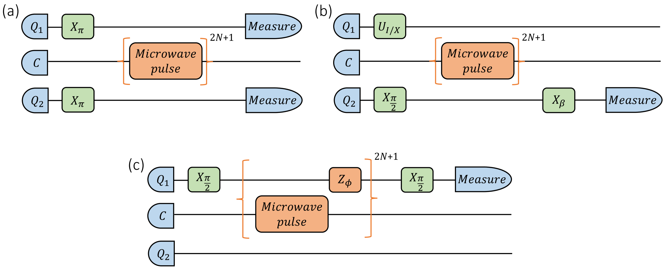
IV.5 Fast calibration of controlled-Z gates
After fine-tuning the qubit frequency, we need to recalibrate CZ gates related to it. The main parameters for calibrating the CZ gates are microwave frequency, microwave amplitude, and dynamic phase of the two relevant qubits. First, we roughly determine the microwave frequency and amplitude through the circuit in Figure 5(a) with typically set to 0. Within this circuit, the two qubits and are initially set at . We first flip these two qubits by applying pulse . Then, we apply the microwave pulse once, and after that, we measure the probability of two qubits returning to the state. In the process of applying microwave pulses, and states will be exchanged, and we try to find the microwave pulse parameters to maximize the probability back to for the ending state. Then, we fine-tune the microwave amplitude by implementing circuit (a) again. To amplify the errors caused by the parameters, we superimpose CZ gates, with this time. As the conditional phase is relatively sensitive to the frequency, we fine-tune the microwave frequency through the circuit in Figure 5(b). When the of changes, the probability of , or the first qubit, changes as follows:
| (7) | |||
| (8) |
By fitting and obtaining and , we can get the conditional phase . The optimal microwave frequency is the frequency at which is satisfied. We then repeat the circuit (a) again to calibrate the microwave amplitude further with a large . The optimal microwave amplitude is the amplitude that makes the probability of the state closest to 1. The dynamic phase of the two relevant qubits can be calibrated through the circuit in Figure 5(c). We first change the dynamic phase of and find the point where the probability of the state is closest to 1 to complete the dynamic phase compensation for . This process is repeated for subsequently with and applied at in circuit (c).
IV.6 Parallel calibration of controlled-Z gate parameters with back probability
When we calibrate CZ gate parameters by means of amplifying errors through the superposition of multiple layers of CZ gate circuits, we can attain a high level of fidelity for most CZ gates. To further refine the gate parameters, we resort to the Nelder-Mead algorithm to continue to search for CZ gate parameters. Particularly, for each local CZ gate, we input , implement a random sequence of two-qubit Clifford gates, and record the probability of the final state back to . Each two-qubit Clifford gate is decomposed into CZ and single-qubit gates in implementation. Additionally, we alternate running the same set of random circuits with the reference and iterative parameters. The difference between their outcomes is used as the target function of the Nelder-Mead algorithm to mitigate environmental influence. To quickly calibrate a set of CZ gates where no two gates share a common qubit, we execute the above procedure in parallel for each local CZ gate. Each gate is calibrated independently using its own back probability. This parallel calibration method typically yields better gate parameters than the parameter scanning approach described in the previous subsection.
IV.7 Fidelity and correlation analysis of depolarizing and correlated noise
In this part, we establish a simple but physical noise model to explain the experimental results. Note that CAB faithfully evaluates the process fidelity of quantum gates [33]. We consider how the process fidelity behaves under a combination of local depolarizing noise and gate interaction. Particularly, for a unitary gate , we consider the following noise model.
| (9) |
where is a depolarizing noise on the -th gate with parameter such that
| (10) |
Here, is the dimension of gate , and is the identity operator on this subsystem. The noise is a correlated noise among all local gates , modeled as a unitary evolution:
| (11) |
The form of incorporates both decoherence on individual gates and interactions between gates. The decoherence on each gate is set as a depolarizing type, which is a standard setting in studies of near-term quantum devices [3, 4, 5, 28]. Different from previous works, we introduce an additional interaction term , which makes the noise model more physical. The form of depends on the implemented gate , which will be specified later. When considering the action of on a subsystem , the remainder of the system is treated as a maximally mixed state or a thermalized state at infinite temperature. That is, for state on subsystem ,
| (12) |
Here, is the restriction of to , is the complementary subsystem of , is the dimension of , and is the identity operator on .
Since the gate comprises gates , we use to denote the whole system. Given a subset , we can represent a part of the gate , , whose fidelity is given by and denoted as . Note that the process fidelity has an expression where is a maximally entangled state on two copies of the system. Through direct calculation, we have that
| (13) |
where is a subset of , is the complementary set of in , and are the dimensions of subsystems and , respectively, and
| (14) |
Note that is the complementary set of in . From Eq. (13), we can obtain the global fidelity and local gate fidelities, and hence evaluate the correlation and investigate how fidelities depend on noise parameters.
In our experiments, we mainly consider the parallel CZ gate . Based on experimental observations, the correlated noise mainly arises from the coupling among qubits. Particularly, we consider a simplified noise model where only one qubit from each CZ gate couples with each other. Without loss of generality, we set this qubit as . Meanwhile, the Hamiltonian of the correlated noise only contains two local terms while the strength between and is set as . Thus, the correlated noise is
| (15) |
The strength parameter is determined by , where is the evolution time, and is the coupling strength between two qubits. In our experiments, corresponds to the two-qubit gate time, which is 110ns. For two physically isolated qubits, their coupling strength is typically less than 0.3 MHz, resulting in less than 0.033 for two uncorrelated gates. For two coupled qubits, can be on the order of 0.1.
Substituting Eq. (15) into Eq. (13) gives the global fidelity and local CZ gate fidelities. We provide the results when and , which relates to our correlation benchmarking and gate optimization results. More general cases can be straightforwardly obtained using Eq. (13).
When , the fidelities of the two local CZ gates are
| (16) | ||||
| (17) |
The global fidelity of the two CZ gates is
| (18) |
The above gives the correlation when only two CZ gates correlate with each other via the coupling:
| (19) |
In the limit that and are close to , is approximately . Then, the correlation is approximately . Given the value of as 0.033 and 0.1, the correlation values take 0.001 and 0.01, respectively. This is consistent with our experimental results.
When , we give the fidelities of the three local CZ gates, the fidelities of each pair of CZ gates, and the global fidelity.
| (20) | ||||
| (21) | ||||
| (22) |
| (23) |
| (24) |
| (25) |
| (26) |
Here, and . In this case, the correlation between the first and second local CZ gates is given by
| (27) |
Note that when and are close to , the first term in the formula of fidelities dominates, and we get the above approximation. It is interesting that the sign of the correlation depends on . A negative correlation value implies that one of and is larger than .
To further investigate how the correlation depends on parameters , and , we fix with values in and depict the correlation with respect to and . The results are available in Figure 6.
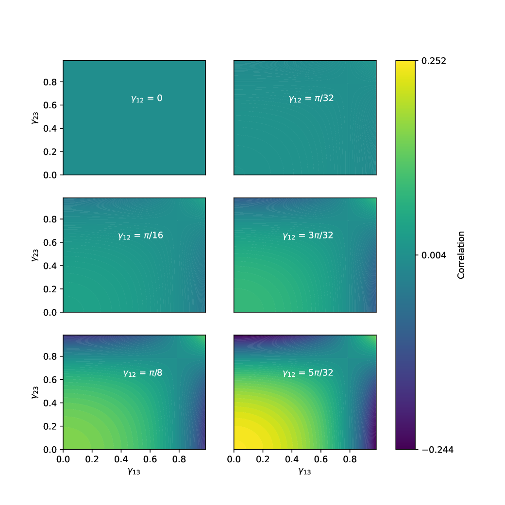
From the expressions in Eqs. (19) and (27), we observe a natural result that the correlation between two gates always increases with their own coupling strength. In the two-gate coupling case, the correlation is , which increases monotonically with . In the three-gate coupling case, the numerator of the correlation is proportional to , which also increases monotonically with . Thus, the correlation magnitude directly reflects the coupling strength.
Examining the sign of the correlation reveals distinct behaviors. If only two CZ gates are coupled, their correlation is always positive. However, in a three-gate coupling scenario, the situation changes. The correlation is still positive for a low-strength correlated noise when all parameters are less than . Nonetheless, if two CZ gates exhibit strong coupling, one of the CZ gates will have a negative correlation with the third CZ gate. From Eq. (27) and Figure 6, we can see that the negativity becomes particularly pronounced when one coupling is weak while the other is strong. This characteristic is useful for identifying the strongly coupled pair of gates.
Beyond correlation analysis, the dependence of local gate fidelities and global fidelity on the coupling strength helps explain the differences between these two types of fidelities in gate optimization. In the case of , this difference is small. Both kinds of fidelities are proportional to , and optimization naturally reduces to improve performance. Nonetheless, for the three-gate coupling model, the situation can be different. Each local fidelity depends only on two coupling parameters. When optimizing , the coupling parameters and tend to be smaller to make higher and make the correlation weaker. However, given a fixed , the decrease of or can also decrease or . For instance, . When , the decrease of makes also decrease. This creates a competition between optimizing one local fidelity and another, often leading to the optimization being trapped in a local region. In contrast, global fidelity incorporates all coupling parameters, allowing the optimization process to simultaneously reduce all coupling strengths.
References
- [1] D. Aharonov, M. Ben-Or, R. Impagliazzo, and N. Nisan, ”Limitations of noisy reversible computation (1996), quant - ph/9611028”, URL https://arxiv.org/abs/quant-ph/9611028
- [2] A. Müller - Hermes, D. Stilck França, and M. M. Wolf, ”Journal of Mathematical Physics 57, 022202 (2016)”, ISSN 0022 - 2488, URL https://doi.org/10.1063/1.4939560
- [3] D. Stilck França and R. García - Patrón, ”Nature Physics 17, 1221 (2021)”, ISSN 1745 - 2481, URL https://doi.org/10.1038/s41567 - 021 - 01356 - 3
- [4] D. Aharonov, X. Gao, Z. Landau, Y. Liu, and U. Vazirani, ”in Proceedings of the 55th Annual ACM Symposium on Theory of Computing (Association for Computing Machinery, New York, NY, USA, 2023), STOC 2023”, pp. 945 - 957, ISBN 9781450399135, URL https://doi.org/10.1145/3564246.3585234
- [5] Y. Yan, Z. Du, J. Chen, and X. Ma, ”Limitations of noisy quantum devices in computational and entangling power (2023), 2306.02836”, URL https://arxiv.org/abs/2306.02836
- [6] L. Egan, D. M. Debroy, C. Noel, A. Risinger, D. Zhu, D. Biswas, M. Newman, M. Li, K. R. Brown, M. Cetina, et al., ”Nature 598, 281 (2021)”, ISSN 1476 - 4687, URL https://doi.org/10.1038/s41586 - 021 - 03928 - y
- [7] M. Gong, X. Yuan, S. Wang, Y. Wu, Y. Zhao, C. Zha, S. Li, Z. Zhang, Q. Zhao, Y. Liu, et al., ”National Science Review 9, nwab011 (2021)”, ISSN 2095 - 5138, URL https://doi.org/10.1093/nsr/nwab011
- [8] L. Postler, S. Heußen, I. Pogorelov, M. Rispler, T. Feldker, M. Meth, C. D. Marciniak, R. Stricker, M. Ringbauer, R. Blatt, et al., ”Nature 605, 675 (2022)”, ISSN 1476 - 4687, URL https://doi.org/10.1038/s41586 - 022 - 04721 - 1
- [9] Y. Zhao, Y. Ye, H. - L. Huang, Y. Zhang, D. Wu, H. Guan, Q. Zhu, Z. Wei, T. He, S. Cao, et al., ”Phys. Rev. Lett. 129, 030501 (2022)”, URL https://link.aps.org/doi/10.1103/PhysRevLett.129.030501
- [10] R. Acharya, I. Aleiner, R. Allen, T. I. Andersen, M. Ansmann, F. Arute, K. Arya, A. Asfaw, J. Atalaya, R. Babbush, et al., ”Nature 614, 676 (2023)”, ISSN 1476 - 4687, URL https://doi.org/10.1038/s41586 - 022 - 05434 - 1
- [11] A. Y. Kitaev, ”Russian Mathematical Surveys 52, 1191 (1997)”, URL https://dx.doi.org/10.1070/RM1997v052n06ABEH002155
- [12] D. Aharonov and M. Ben-Or, ”in Proceedings of the Twenty-Ninth Annual ACM Symposium on Theory of Computing (Association for Computing Machinery, New York, NY, USA, 1997), STOC ’97”, pp. 176 - 188, ISBN 0897918886, URL https://doi.org/10.1145/258533.258579
- [13] E. Knill, R. Laflamme, and W. H. Zurek, ”Proceedings of the Royal Society of London. Series A: Mathematical, Physical and Engineering Sciences 454, 365 (1998)”, URL https://royalsocietypublishing.org/doi/abs/10.1098/rspa.1998.0166
- [14] R. Barends, J. Kelly, A. Megrant, A. Veitia, D. Sank, E. Jeffrey, T. C. White, J. Mutus, A. G. Fowler, B. Campbell, et al., ”Nature 508, 500 (2014)”, URL https://doi.org/10.1038/nature13171
- [15] I. L. Chuang and M. A. Nielsen, ”Journal of Modern Optics 44, 2455 (1997)”, URL https://www.tandfonline.com/doi/abs/10.1080/09500349708231894
- [16] S. T. Flammia and Y. - K. Liu, ”Phys. Rev. Lett. 106, 230501 (2011)”, URL https://link.aps.org/doi/10.1103/PhysRevLett.106.230501
- [17] J. Emerson, R. Alicki, and K. Zyczkowski, ”Journal of Optics B: Quantum and Semiclassical Optics 7, S347 (2005)”, URL https://doi.org/10.1088/1464 - 4266/7/10/021
- [18] J. Emerson, M. Silva, O. Moussa, C. Ryan, M. Laforest, J. Baugh, D. G. Cory, and R. Laflamme, ”Science 317, 1893 (2007)”, URL https://www.science.org/doi/abs/10.1126/science.1145699
- [19] E. Knill, D. Leibfried, R. Reichle, J. Britton, R. B. Blakestad, J. D. Jost, C. Langer, R. Ozeri, S. Seidelin, and D. J. Wineland, ”Phys. Rev. A 77, 012307 (2008)”, URL https://link.aps.org/doi/10.1103/PhysRevA.77.012307
- [20] E. Magesan, J. M. Gambetta, and J. Emerson, ”Phys. Rev. Lett. 106, 180504 (2011)”, URL https://link.aps.org/doi/10.1103/PhysRevLett.106.180504
- [21] E. Magesan, J. M. Gambetta, and J. Emerson, ”Phys. Rev. A 85, 042311 (2012)”, URL https://link.aps.org/doi/10.1103/PhysRevA.85.042311
- [22] E. Magesan, J. M. Gambetta, B. R. Johnson, C. A. Ryan, J. M. Chow, S. T. Merkel, M. P. da Silva, G. A. Keefe, M. B. Rothwell, T. A. Ohki, et al., ”Phys. Rev. Lett. 109, 080505 (2012)”, URL https://link.aps.org/doi/10.1103/PhysRevLett.109.080505
- [23] D. C. McKay, S. Sheldon, J. A. Smolin, J. M. Chow, and J. M. Gambetta, ”Phys. Rev. Lett. 122, 200502 (2019)”, URL https://link.aps.org/doi/10.1103/PhysRevLett.122.200502
- [24] T. J. Proctor, A. Carignan - Dugas, K. Rudinger, E. Nielsen, R. Blume - Kohout, and K. Young, ”Phys. Rev. Lett. 123, 030503 (2019)”, URL https://link.aps.org/doi/10.1103/PhysRevLett.123.030503
- [25] A. Erhard, J. J. Wallman, L. Postler, M. Meth, R. Stricker, E. A. Martinez, P. Schindler, T. Monz, J. Emerson, and R. Blatt, ”Nature Communications 10, 5347 (2019)”, ISSN 2041 - 1723, URL https://doi.org/10.1038/s41467 - 019 - 13068 - 7
- [26] J. Hines, M. Lu, R. K. Naik, A. Hashim, J. - L. Ville, B. Mitchell, J. M. Kriekebaum, D. I. Santiago, S. Seritan, E. Nielsen, et al., ”Phys. Rev. X 13, 041030 (2023)”, URL https://link.aps.org/doi/10.1103/PhysRevX.13.041030
- [27] Q. Zhu, S. Cao, F. Chen, M. - C. Chen, X. Chen, T. - H. Chung, H. Deng, Y. Du, D. Fan, M. Gong, et al., ”Science Bulletin 67, 240 (2022)”, ISSN 2095 - 9273, URL https://www.sciencedirect.com/science/article/pii/S2095927321006733
- [28] A. Morvan, B. Villalonga, X. Mi, S. Mandrá, A. Bengtsson, P. V. Klimov, Z. Chen, S. Hong, C. Erickson, I. K. Drozdov, et al., ”Nature 634, 328 (2024)”, ISSN 1476 - 4687, URL https://doi.org/10.1038/s41586 - 024 - 07998 - 6
- [29] D. C. McKay, I. Hincks, E. J. Pritchett, M. Carroll, L. C. G. Govia, and S. T. Merkel, ”Benchmarking quantum processor performance at scale (2023), 2311.05933”, URL https://arxiv.org/abs/2311.05933
- [30] S. A. Moses, C. H. Baldwin, M. S. Allman, R. Ancona, L. Ascarrunz, C. Barnes, J. Bartolotta, B. Bjork, P. Blanchard, M. Bohn, et al., ”Phys. Rev. X 13, 041052 (2023)”, URL https://link.aps.org/doi/10.1103/PhysRevX.13.041052
- [31] M. K. Joshi, C. Kokail, R. van Bijnen, F. Kranzl, T. V. Zache, R. Blatt, C. F. Roos, and P. Zoller, ”Nature 624, 539 (2023)”, ISSN 1476 - 4687, URL https://doi.org/10.1038/s41586 - 023 - 06768 - 0
- [32] D. Bluvstein, S. J. Evered, A. A. Geim, S. H. Li, H. Zhou, T. Manovitz, S. Ebadi, M. Cain, M. Kalinowski, D. Hangleiter, et al., ”Nature 626, 58 (2024)”, URL https://doi.org/10.1038/s41586 - 023 - 06927 - 3
- [33] Y. Zhang, W. Yu, P. Zeng, G. Liu, and X. Ma, ”Photon. Res. 11, 81 (2023)”, URL https://opg.optica.org/prj/abstract.cfm?URI = prj - 11 - 1 - 81
- [34] M. Cerezo, A. Arrasmith, R. Babbush, S. C. Benjamin, S. Endo, K. Fujii, J. R. McClean, K. Mitarai, X. Yuan, L. Cincio, et al., ”Nature Reviews Physics 3, 625 (2021)”, URL https://doi.org/10.1038/s42254 - 021 - 00348 - 9
- [35] R. Raussendorf, D. E. Browne, and H. J. Briegel, ”Physical Review A 68 (2003)”, URL https://doi.org/10.1103%2Fphysreva.68.022312
- [36] M. Hein, J. Eisert, and H. J. Briegel, ”Phys. Rev. A 69, 062311 (2004)”, URL https://link.aps.org/doi/10.1103/PhysRevA.69.062311
- [37] J. A. Nelder and R. Mead, ”The Computer Journal 7, 308 (1965)”, ISSN 0010 - 4620, URL https://doi.org/10.1093/comjnl/7.4.308
- [38] See Supplementary Material for more detailed experimental data of the comparison between character-average benchmarking and cycle benchmarking, the fluctuation analysis of the experimental results, and additional benchmarking and optimization results, which includes references [33, 25].
- [39] M. A. Rol, C. C. Bultink, T. E. O’Brien, S. R. de Jong, L. S. Theis, X. Fu, F. Luthi, R. F. L. Vermeulen, J. C. de Sterke, A. Bruno, et al., “Phys. Rev. Appl. 7, 041001 (2017)”, URL https://link.aps.org/doi/10.1103/PhysRevApplied.7.041001
- [40] D. Gottesman, “Stabilizer codes and quantum error correction (California Institute of Technology, 1997)”, URL https://arxiv.org/abs/quant - ph/9705052
- [41] A. W. Cross, J. M. Gambetta, D. Maslov, P. Rall, and T. J. Yoder, “Nature 627, 778 (2024)”, URL https://doi.org/10.1038/s41586-024-07107-7
- [42] Y. Wu, W. - S. Bao, S. Cao, F. Chen, M. - C. Chen, X. Chen, T. - H. Chung, H. Deng, Y. Du, D. Fan, et al., “Phys. Rev. Lett. 127, 180501 (2021)”, URL https://link.aps.org/doi/10.1103/PhysRevLett.127.180501
- [43] R. Barends, C. M. Quintana, A. G. Petukhov, Y. Chen, D. Kafri, K. Kechedzhi, R. Collins, O. Naaman, S. Boixo, F. Arute, et al., “Phys. Rev. Lett. 123, 210501 (2021)”, URL https://link.aps.org/doi/10.1103/PhysRevLett.123.210501
- [44] S. Boixo, in “APS March Meeting Abstracts (2017), vol. 2017 of APS Meeting Abstracts, p. A19.005
- [45] F. Arute, K. Arya, R. Babbrusch, D. Bacon, J. C. Bardin, R. Barends, R. Biswas, S. Boixo, F. G. S. L. Brandao, D. A. Buell, et al., “Nature 574, 505 (2019)”, ISSN 1476 - 4687, URL https://doi.org/10.1038/s41586 - 019 - 1666 - 5
- [46] H. Xu, W. Liu, Z. Li, J. Han, J. Zhang, K. Linghu, Y. Li, M. Chen, Z. Yang, J. Wang, et al., “Chinese Physics B 30, 044212 (2021)”, URL https://dx.doi.org/10.1088/1674 - 1056/abf03a