Optimizing Server Locations for Stochastic Emergency Service Systems

Abstract

This paper presents a new model for solving the optimal server location problem in a stochastic system that accounts for unit availability, heterogeneity, and interdependencies. We show that this problem is NP-hard and derive both lower and upper bounds for the optimal solution by leveraging a special case of the classic $p$-Median problem. To overcome the computational challenges, we propose two Bayesian optimization approaches: (i) a parametric method that employs a sparse Bayesian linear model with a horseshoe prior (SparBL), and (ii) a non-parametric method based on a Gaussian process surrogate model with $p$-Median as mean prior (GP-$p$M). We prove that both algorithms achieve sublinear regret rates and converge to the optimal solution, with the parametric approach demonstrating particular effectiveness in high-dimensional settings. Numerical experiments and a case study using real-world data from St. Paul, Minnesota emergency response system show that our approaches consistently and efficiently identify optimal solutions, significantly outperforming the $p$-Median solution and other baselines.

Keywords:emergency service system; facility location; Bayesian optimization; service operations

1 Introduction

Over the past 50 years, a large literature has appeared on operations research models for emergency services deployment (Green & Kolesar, 2004). One of the most often cited and widely applied models is the hypercube queuing model for spatially distributed emergency service units (Larson, 1974, 1975). For discussions of the early literature including the hypercube model, see Kolesar & Swersey (1986), Swersey (1994), and Iannoni & Morabito (2023). The hypercube framework models a server-to-customer service system in which emergency units travel to incident locations, typical in fire, police, and emergency medical service (EMS) operations. Unlike traditional customer-to-server systems, the main challenge arises from the heterogeneity of servers, primarily due to their distinct geographic locations. Each unit is stationed at a predefined location and is dispatched in response to calls arising from spatially distributed demand. Once dispatched, a unit becomes unavailable for a random service duration. The model aims to evaluate key performance measures such as the average response time and coverage probabilities.

In this paper, we develop a prescriptive model to determine optimal server locations in stochastic emergency service systems. Unlike the descriptive hypercube model, our approach optimizes unit placement under a specified dispatching policy to minimize the mean response time. While our primary goal is to minimize average response time, our model also accommodates alternative objectives, such as meeting time-based service targets, as demonstrated in the St. Paul case study. We define response time as the sum of turnout time, which is the time from when the call is received until the response unit begins traveling, and the travel time to the incident location. In EMS, turnout time reflects the delay before an ambulance departs the station. In police systems, units are typically patrolling, making turnout time negligible. Response time is a critical performance measure in emergency systems: in EMS and fire systems, shorter response times improve patient survival, while in police systems, they increase the probability of apprehension.

A central feature of our model is its incorporation of stochastic unit availability, heterogeneity, and interdependencies. Some of these factors are often neglected in traditional models such as the $p$-Median model (Hakimi, 1964) and covering-based models (Toregas et al., 1971; Church & ReVelle, 1974; Daskin, 1983), which typically assume full availability or uniform utilization across units. Specifically, the contributions of this paper are as follows:

• We study the problem of locating emergency service units while accounting for differences in location-based performance, stochastic unit availability due to ongoing service, and interdependencies across the system. We show that the resulting optimization problem is NP-hard. We establish a lower bound using the optimal solution value in a $p$-Median problem (Hakimi, 1964) and also derive a feasible upper bound.

• We develop a Bayesian optimization (BO) approach with a parametric model that employs a sparse Bayesian linear regression with a horseshoe prior. This method introduces: (i) a sparsity-inducing surrogate that automatically identifies relevant features through hierarchical shrinkage, (ii) a submodular relaxation technique to transform the binary quadratic program (BQP) acquisition function into an efficiently solvable graph-cut formulation. The horseshoe prior’s self-adaptive properties yield a regret bound $\mathcal{O}(Ws_{0}\sqrt{T\log D})$ dependent on true sparsity $s_{0}$.

• We also propose a non-parametric alternative based on a classical Gaussian Process (GP) surrogate. While conventional GP-based Bayesian optimization methods (Frazier, 2018b) are designed for continuous domains and are ill-suited for combinatorial settings, we adapt the framework through several specialized techniques. These include a custom-designed kernel function, trust-region constraints to maintain feasibility, a restart mechanism, and an adaptive swapping-based search strategy. We prove that this method achieves sublinear regret rates and converges to the optimal solution.

• Extensive numerical experiments show that both of our approaches consistently outperform benchmark methods. We further apply them to an ambulance location problem in St. Paul, Minnesota, using real-world data, and demonstrate that both algorithms converge rapidly to the global optimum. Our framework also accommodates alternative objectives beyond standard performance metrics. For example, we formulate and solve the problem of minimizing the fraction of calls exceeding a specified response time threshold (Blackwell & Kaufman, 2002; Maxwell et al., 2010), illustrating the method’s flexibility while maintaining computational efficiency.

The remainder of this paper is organized as follows. In §2, we review the relevant literature. In §3, we define the problem in mathematical terms and show its relationship to the $p$-Median problem. In §4, we introduce the parametric sparse Bayesian linear model. In §5, we develop the non-parametric GP-based BO algorithm. In §6, we investigate the performance of the proposed algorithm through numerical experiments. In §7, we apply our solution method to the real data of St. Paul, Minnesota emergency service system and discuss managerial insights. Finally, in §8, we discuss conclusions.

2 Literature Review

2.1 Location Models in Emergency Service Systems

This section reviews literature on location problems in emergency service systems. Ahmadi-Javid et al. (2017) provides an extensive overview of healthcare facility location models, while Ingolfsson (2013) focuses on empirical studies and stochastic modeling for emergency medical services. Location problems are typically classified as either discrete or continuous. Discrete models assign units to predefined sites (Berman et al., 2007), while continuous models allow placement anywhere within a region (Baron et al., 2008). Our work focuses on the discrete setting, particularly relevant to emergency services. Daskin (2008) offers a detailed survey of such problems.

Among the most prominent are the $p$-median and covering models, which have formed the backbone of traditional emergency service location planning. The $p$-median model (Hakimi, 1964) chooses $p$ facility sites to minimize total distance or travel time to demand points. Covering models, including the location set covering model (LSCM) of Toregas et al. (1971) and the maximal covering location problem (MCLP) of Church & ReVelle (1974), aim to ensure that as many demands as possible are covered within a specified response time or distance. These classic models provided a foundation for emergency facility deployment by focusing on geographic coverage and average travel metrics. However, they fail to reflect the stochastic realities of emergency service systems, where both demand and service times are random, and units are often unavailable due to ongoing calls.

To better reflect real emergency systems, researchers extended basic models to account for unit availability and reliability. Probabilistic covering models like MEXCLP (Daskin, 1983) estimate expected coverage using busy fractions, while MALP (ReVelle & Hogan, 1989) ensures zones are covered with high probability. Though more realistic than deterministic models, these approaches often treat busy probabilities as fixed and ignore dependencies.

2.2 Spatial Hypercube Model

Researchers have proposed models that consider the stochastic nature of the system. The problem we consider is the same as that addressed in the spatial hypercube model, developed by (Larson, 1974, 1975). But as stated earlier, in contrast to the hypercube model which is descriptive, our model finds the optimal set of unit locations. The hypercube model determines average system-wide response time given a set of unit locations, and has been widely cited and applied to police patrol problems (Chaiken, 1978) and to locating ambulances (Brandeau & Larson, 1986). It has also been used as input to the maximal expected covering location problem by Batta et al. (1989), and in network and discrete location problems by Daskin (2011). The hypercube necessitates solving $2^{p}$ equations where $p$ is the number of servers. For larger systems, Larson (1975) developed an approximation algorithm that requires only solving $p$ equations.

Ghobadi et al. (2021) surveyed papers that integrate location models and the hypercube model, and identified several papers that seek to minimize average response time in the hypercube setting, but in contrast to our approach, these papers do not find optimal solutions. These papers are Geroliminis et al. (2004) a heuristic approach, Geroliminis et al. (2009), simulation, Geroliminis et al. (2011), a heuristic genetic algorithm, Chanta et al. (2011), tabu search, and Toro-D´ıaz et al. (2013), a genetic algorithm.

The spatial hypercube model has been incorporated into other location models to address stochasticity. For example, Berman et al. (1987) developed two heuristics combining median problems with the hypercube model to solve the stochastic queue $p$-Median problem, while Ingolfsson et al. (2008) proposed an iterative method to determine ambulance locations that minimize fleet size subject to service-level constraints. Unlike these heuristic approaches, we propose a solution method with theoretical performance guarantees, ensuring convergence to the optimal solution with provable regret bounds.

2.3 Bayesian Optimization

Bayesian optimization (BO) (Frazier, 2018a, b) is a technique usually used to optimize objective functions that are expensive or time-consuming to evaluate, and has been used to solve complex, large-scale optimization problems because it efficiently balances exploration and exploitation in the search space. Bayesian optimization has been applied in a wide range of fields, including food safety control (Hu et al., 2010) and drug discovery (Negoescu et al., 2011).

While many Bayesian optimization techniques have been developed for continuous spaces (Frazier, 2018b), using Bayesian optimization for discrete optimization problems as in the current paper is more challenging because it was originally developed for continuous functions, which are generally easier to optimize due to their smooth and predictable nature (Frazier, 2018a). Discrete optimization problems, such as combinatorial optimization problems, are often non-smooth and have a larger number of discrete solutions which makes the optimization process more challenging. Additionally, Gaussian processes (discussed in §5.1), which are commonly used in Bayesian optimization as surrogate models, are not well-suited for discrete spaces, making it difficult to develop accurate models (Williams & Rasmussen, 2006). Therefore, special methods need to be developed to handle optimization in discrete spaces.

Baptista & Poloczek (2018) were among the first to adapt BO to categorical spaces, using a second-order monomial representation with Bayesian linear regression as the surrogate model, while Ru et al. (2020) developed an approach integrating multi-armed bandits with GP-based BO.  Wan et al. (2021) extend this work and introduce the idea of tailored kernels and trust regions. Other significant contributions include Deshwal et al. (2020)’s work on diffusion kernels for discrete objects, Wu et al. (2020)’s variational optimization framework, and Oh et al. (2019)’s GP surrogate model using combinatorial graphs. Despite these developments, existing methods still face three key limitations: (i) lack of theoretical convergence guarantees, (ii) limited scalability in high-dimensional discrete spaces, and (iii) limited applicability to facility location problems.

3 Model

3.1 Problem Formulation

We aim to select $p$ locations from a set of $N$ candidate sites, denoted by $I$, to minimize the average response time under a specified dispatching policy. The service region is partitioned into $M$ subregions, represented by the set $J$, where calls in each subregion $j\in J$ arrive according to a Poisson process with rate $\lambda_{j}$. The service time for a unit stationed at location $i$ includes turnout time, travel to the scene, time on scene, and return travel, with an average duration of $1/\mu_{i}$. We assume an exponential distribution for service times for modeling purposes, though our method extends to general service time distributions, as the approximation method developed by Larson (1975) can accommodate such cases, as discussed in §B of the E-Companion.

Under the specified dispatching policy, each call is assigned to an emergency unit based on a fixed assignment rule. We create the fixed assignment rule by specifying a predetermined preference list of units for calls from each subregion. When a call is received from a subregion, the most preferred available unit on the list is dispatched. If the preference list is based on distance to the call, the closest available unit would be dispatched. If all units are busy when the call arrives, we assume that it is responded to by a unit from an adjacent jurisdiction, which is the usual mutual aid policy in emergency service systems. As mentioned earlier, response time is the sum of the unit turnout time and travel time. The term $t_{ij}$ represents the expected travel time from server location $i$ to call location $j$, and $\tau_{i}$ denotes the average turnout time from location $i$.

We define binary variables $x_{i}$ to represent the occupancy of locations, where $x_{i}=1$ indicates that location $i$ is occupied by a unit, and $x_{i}=0$ denotes an empty location $i$. The vector $\boldsymbol{x}=\{x_{1},\cdots,x_{N}\}\in\{0,1\}^{N}$ is the set of unit locations. We use boldface symbols for vectors and matrices in the rest of the paper. Our objective is to determine the optimal set of unit locations $\boldsymbol{x}^{*}$ that minimizes the system-wide mean response time. To achieve this, we solve an integer program that we call $p$-MRT.

$$\text{OPT}_{R}=\min_{\boldsymbol{x}} \sum_{i\in I}\sum_{j\in J}(\tau_{i}+t_{ij})q_{ij}(\boldsymbol{x})\qquad\text{\emph{({$p$-MRT})}}$$ (1a)

s.t. $$\sum_{i\in I}x_{i}=p,$$ (1b)

$$q_{ij}(\boldsymbol{x})=\frac{\sum_{\boldsymbol{b}\in S_{ij}(\boldsymbol{x})}\lambda_{j}P(\boldsymbol{b})}{\sum_{j\in J}\lambda_{j}\left(1-\Pi\right)},\forall i\in I,\forall j\in J,$$ (1c)

$$x_{i}\in\{0,1\},\forall i\in I.$$ (1d)

In the above formulation, $q_{ij}(\boldsymbol{x})$ is the proportion of calls originating from subregion $j$ that are serviced by the unit located at $i$, given a unit configuration $\boldsymbol{x}$. The state of all $p$ units is represented by $\boldsymbol{b}=\{b_{1},\cdots,b_{p}\}\in\{0,1\}^{p}$, where $b_{k}=0$ indicates unit $k$ is available, and $b_{k}=1$ means unit $k$ is busy. The probability of being in state $\boldsymbol{b}$ is $P(\boldsymbol{b})$, and the blocking probability for calls from sub-region $j$ is $\Pi$. Furthermore, $S_{ij}(\boldsymbol{x})$ denotes the set of states where the unit located at location $i$ is assigned to calls from subregion $j$. We note that the determination of $q_{ij}(\boldsymbol{x})$ depends on $P(\boldsymbol{b})$ and $\Pi$, which requires solving the balance equations of the spatial hypercube model of Larson (1974). For all $\boldsymbol{b}$, the balance equations are:

$$P(\boldsymbol{b})\Bigg{[}\underbrace{\sum_{j\in J}\lambda_{j}}_{\text{arrival}}+\underbrace{\sum_{k=1}^{p}b_{k}\mu_{k}}_{\text{service completion}}\Bigg{]}=\underbrace{\sum_{\boldsymbol{b}^{\prime}:H(\boldsymbol{b},\boldsymbol{b}^{\prime})^{+}=1}P(\boldsymbol{b}^{\prime})r(\boldsymbol{b},\boldsymbol{b}^{\prime})}_{\text{upward transitions}}+\underbrace{\sum_{\boldsymbol{b}^{\prime}:H(\boldsymbol{b},\boldsymbol{b}^{\prime})^{-}=1}P(\boldsymbol{b}^{\prime})\mu_{i(\boldsymbol{b},\boldsymbol{b}^{\prime})}}_{\text{downward transitions}},$$ (2)

where $r(\boldsymbol{b},\boldsymbol{b}^{\prime})$ is the transition rate from state $\boldsymbol{b}$ to state $\boldsymbol{b}^{\prime}$ in the spatial hypercube model, $i(\boldsymbol{b},\boldsymbol{b}^{\prime})$ is the index at which $\boldsymbol{b}$ and $\boldsymbol{b}^{\prime}$ differ, and $H(\boldsymbol{b},\boldsymbol{b}^{\prime})$ is the Hamming distance from $\boldsymbol{b}$ to $\boldsymbol{b}^{\prime}$, which is defined as

$$H(\boldsymbol{b},\boldsymbol{b}^{\prime})=w\left(\left[\boldsymbol{b}\cap\neg\boldsymbol{b}^{\prime}\right]\cup\left[\neg\boldsymbol{b}\cap\boldsymbol{b}^{\prime}\right]\right),$$ (3)

where $\cap$ and $\cup$ are bitwise AND and OR operations, respectively, and $\neg\boldsymbol{b}$ is the logical NOT operation of the binary number representation of state $\boldsymbol{b}$. The function $w(\cdot)$ adds the number of 1s in the binary state representation. Transitions in the spatial hypercube model only take place to adjacent states, i.e., $H(\boldsymbol{b},\boldsymbol{b}^{\prime})=1$. Larson (1974) introduced upward and downward Hamming distances, which are denoted by $H(\boldsymbol{b},\boldsymbol{b}^{\prime})^{+}$ and $H(\boldsymbol{b},\boldsymbol{b}^{\prime})^{-}$, respectively. An upward distance measures the distance to states reached by call arrivals and a downward distance measures the distance to states reached by service completions. Thus,

$$H(\boldsymbol{b},\boldsymbol{b}^{\prime})^{+}=w\left(\left[\boldsymbol{b}\cap\neg\boldsymbol{b}^{\prime}\right]\right),\qquad H(\boldsymbol{b},\boldsymbol{b}^{\prime})^{-}=w\left(\left[\neg\boldsymbol{b}\cap\boldsymbol{b}^{\prime}\right]\right).$$ (4)

Clearly, $H(\boldsymbol{b},\boldsymbol{b}^{\prime})=H(\boldsymbol{b},\boldsymbol{b}^{\prime})^{+}+H(\boldsymbol{b},\boldsymbol{b}^{\prime})^{-}$. To evaluate the actual objective function $f$ is time-consuming as it requires solving the transition matrix for a model with $2^{p}$ states, where $p$ is the number of units.

Theorem 1.

The $p$-MRT problem is NP-hard.

The proof of this theorem is in §D.1 of the E-Companion. To evaluate the objective function, we use the efficient approximation algorithm for the hypercube model proposed by Larson (1975). This method allows us to handle large-scale instances that are computationally prohibitive under the exact model and can accommodate non-Markovian service time distributions. Further details are provided in Section B of the E-Companion.

3.2 Lower and Upper Bounds

This section establishes lower and upper bounds for the optimal solution of the $p$-MRT problem by establishing its connection to the classical $p$-Median problem. The $p$-Median problem (Hakimi, 1964) determines the minimum average response time to all calls while assuming units are always available.

We first develop a lower bound. In the $p$-Median problem, binary variables $x_{i}\in\{0,1\}$ indicate whether a unit is located at position $i$, similar to the variables in the $p$-MRT problem. Additionally, we introduce binary variables $y_{ij}\in\{0,1\}$ to indicate the assignment of calls from subregion $j$ to the unit located at location $i$. We denote the optimal solution to the $p$-Median problem as $(\boldsymbol{\widehat{x}}^{*},\boldsymbol{\widehat{y}}^{*})$. The objective of the $p$-Median model is to minimize the total call-weighted response time, where $w_{j}$ is the weight for subregion $j$. We have

$$\text{OPT}_{M} =\min_{\boldsymbol{x},\boldsymbol{y}}\sum_{i\in I}\sum_{j\in J}w_{j}(\tau_{i}+t_{ij})y_{ij}\qquad\text{\emph{({$p$-Median})}}$$ (5a)

s.t. $$\sum_{i\in I}x_{i}=p,$$ (5b)

$$\sum_{i\in I}y_{ij}=1,\forall j\in J,$$ (5c)

$$y_{ij}\leq x_{i},\forall i\in I,\forall j\in J,$$ (5d)

$$y_{ij}\in\{0,1\},\forall i\in I,\forall j\in J,$$ (5e)

$$x_{i}\in\{0,1\},\forall i\in I.$$ (5f)

Constraint (5c) requires that each subregion is assigned to a unit, and Constraint (5d) requires that calls in subregion $j$ are only assigned to an occupied location. The $p$-Median problem does not include the service rate because it assumes that all units are always available.

We next show that a special case of $p$-Median provides a lower bound for the optimal value of $p$-MRT.

Theorem 2.

The optimal value to the $p$-Median problem is a lower bound for the optimal value of the $p$-MRT problem when $w_{j}=\lambda_{j}/\sum_{k\in J}\lambda_{k}$, i.e.,

$$\text{OPT}_{R}\geq\text{OPT}_{M}.$$

The detailed proof of Theorem 2 is in §D.2. Next, we derive an upper bound, as presented in Lemma 3.

Lemma 3.

By setting $w_{j}=\lambda_{j}/\sum_{k\in J}\lambda_{k}$, applying the optimal solution $\boldsymbol{\widehat{x}}^{*}$ obtained from the $p$-Median problem to the $p$-MRT problem always provides an upper bound on the optimal value of the $p$-MRT problem.

Given that the optimal solution $\boldsymbol{\widehat{x}}^{*}$ is always a feasible solution for the $p$-MRT problem, we leverage this to establish an upper bound on the optimal value of the $p$-MRT problem, which is a minimization problem.

Next, we present two BO solutions for $p$-MRT. We begin by introducing sparse Bayesian linear regression with a horseshoe prior, a parametric method that balances strong interpretability and computational efficiency through hierarchical shrinkage. Subsequently, we present the GP-based method, a non-parametric approach widely adopted in BO for its flexibility.

4 Parametric Surrogate: Sparse Linear Model with Horseshoe Prior

4.1 Bayesian Linear Model with Horseshoe Prior

In this section, we propose a parametric surrogate model based on sparse Bayesian linear regression with a horseshoe prior (SparBL), motivated by Baptista & Poloczek (2018). This model facilitates identifying influential locations and interaction effects critical for modeling unit placement decisions in emergency service systems. The surrogate model is given by:

$$f_{\alpha}(\mathbf{x})=\alpha_{0}+\sum_{j}\alpha_{j}x_{j}+\sum_{i,j>i}\alpha_{ij}x_{i}x_{j}.$$ (6)

where $\mathbf{x}\in\mathcal{D}\subseteq\{0,1\}^{N}$ is a binary vector indicating the selected facility locations, and the model includes both main effects and pairwise interaction terms. Although the interaction terms are quadratic in $\mathbf{x}$, the model is linear in the parameter vector $\alpha=(\alpha_{i},\alpha_{ij})\in\mathbb{R}^{D}$ with $D=1+N+\binom{N}{2}$. Given observations $\{(\mathbf{x}^{(t)},y^{(t)}(\mathbf{x}^{(t)}))\}_{t=1}^{T}$ and model (6), we assume $y^{(t)}(\mathbf{x}^{(t)})=f_{\alpha}(\mathbf{x}^{(t)})+\varepsilon^{(t)}$ where $\varepsilon^{(t)}\sim\mathcal{N}(0,\sigma^{2})$. Under this model, we have:

$$\mathbf{y}\mid\mathbf{X},\alpha,\sigma \sim\mathcal{N}(\mathbf{X}\alpha,\sigma^{2}\mathbf{I}_{D})$$ (7)

$$\alpha_{k}\mid\beta_{k},\tau,\sigma \sim\mathcal{N}(0,\beta_{k}^{2}\tau^{2}\sigma^{2})\quad k=1,\ldots,D$$

$$\tau,\beta_{k} \sim C^{+}(0,1)\quad k=1,\ldots,D$$

$$\sigma^{2} \sim\sigma^{-2}\text{d}\sigma^{2}.$$

Here, the coefficient vector $\alpha$ is assigned a hierarchical horseshoe prior through a global-local shrinkage structure. Each coefficient $\alpha_{k}$ is normally distributed with variance scaled by a global parameter $\tau^{2}$ and a local parameter $\beta_{k}^{2}$, both of which follow independent half-Cauchy distributions denoted by $C^{+}(0,1)$ with probability density function $p(z)=\frac{2}{\pi(1+z^{2})}$ for $z>0$. We are using an improper prior for $\sigma^{2}$ with density proportional to $1/\sigma^{2}$ over $(0,\infty)$ and $\text{d}\sigma^{2}$ refers to the Lebesgue measure over the continuous domain of $\sigma^{2}$.

This horseshoe prior induces strong sparsity by shrinking irrelevant coefficients $\alpha_{k}$ toward zero while allowing significant effects to remain unregularized. The global parameter $\tau$ controls the overall sparsity level, while each $\beta_{k}$ allows local adaptivity. The prior on $\sigma^{2}$ reflects a weakly informative belief about noise variance. This hierarchical prior structure is effective in high-dimensional settings, where most interaction terms are expected to be irrelevant. It avoids overfitting while enabling accurate surrogate modeling of complex functions.

Posterior Distribution

To enable efficient sampling under the horseshoe prior, the half-Cauchy distributions on the local shrinkage parameters $\beta_{k}$ and the global shrinkage parameter $\tau$ are reparameterized using auxiliary variables $\nu_{k}$ and $\xi$, which yield inverse-gamma representations (Makalic & Schmidt, 2016). This reparameterization transforms the hierarchical model into a form where posterior distribution can be expressed in closed form. Under this reparameterization, the full conditional posterior distributions for the model parameters are given by:

$$\alpha \mid\cdot\sim\mathcal{N}(\mathbf{M}^{-1}\mathbf{X}^{T}\mathbf{y},\sigma^{2}\mathbf{M}^{-1}),\quad\mathbf{M}=(\mathbf{X}^{T}\mathbf{X}+\Sigma_{*}^{-1}),\quad\Sigma_{*}=\tau^{2}\text{diag}(\beta_{1}^{2},\ldots,\beta_{D}^{2})$$ (8)

$$\sigma^{2} \mid\cdot\sim\mathcal{IG}\left(\frac{N+D}{2},\frac{(\mathbf{y}-\mathbf{X}\alpha)^{T}(\mathbf{y}-\mathbf{X}\alpha)+\alpha^{T}\Sigma_{*}^{-1}\alpha}{2}\right)$$

$$\beta_{k}^{2} \mid\cdot\sim\mathcal{IG}\left(1,\frac{1}{\nu_{k}}+\frac{\alpha_{k}^{2}}{2\tau^{2}\sigma^{2}}\right)\quad k=1,\ldots,D$$

$$\tau^{2} \mid\cdot\sim\mathcal{IG}\left(\frac{D+1}{2},\frac{1}{\xi}+\frac{1}{2\sigma^{2}}\sum_{k=1}^{D}\frac{\alpha_{k}^{2}}{\beta_{k}^{2}}\right)$$

$$\nu_{k} \mid\cdot\sim\mathcal{IG}\left(1,1+\frac{1}{\beta_{k}^{2}}\right)\quad k=1,\ldots,D$$

$$\xi \mid\cdot\sim\mathcal{IG}\left(1,1+\frac{1}{\tau^{2}}\right).$$

Here, $\mathcal{IG}(a,b)$ denotes the inverse-gamma distribution with shape parameter $a$ and scale parameter $b$. The notation $\mid\cdot$ serves as a shorthand for conditioning on all other relevant variables in the model. The matrix $\mathbf{M}$ captures the posterior precision of the regression coefficients $\alpha$, incorporating both the design matrix $\mathbf{X}$ and the shrinkage structure imposed by $\Sigma_{*}$. The auxiliary variables $\nu_{k}$ and $\xi$ allow the half-Cauchy priors on $\beta_{k}$ and $\tau$ to be expressed as hierarchical inverse-gamma priors, which are conjugate to the Gaussian likelihood. The result is a computationally tractable yet flexible model that automatically performs shrinkage and variable selection.

4.2 Acquisition Function

BO uses an acquisition function to evaluate and prioritize candidate solutions based on the model’s posterior distribution. The acquisition function guides the search by selecting the most promising points to evaluate next. In the non-parametric setting, we adopt Thompson sampling (Thompson, 1935) as the acquisition strategy. Thompson sampling selects a candidate point $\mathbf{x}$ with probability proportional to the likelihood that $\mathbf{x}$ maximizes the unknown objective function. At each iteration $t$, we draw a sample $\alpha_{t}\sim\mathcal{P}(\alpha\mid\mathbf{X},\mathbf{y})$ from the current posterior distribution over model parameters. Using this sampled surrogate model $f_{\alpha_{t}}(x)$, we then seek the maximizer:

$$\arg\max_{\mathbf{x}\in\mathcal{D},\|\mathbf{x}\|_{0}=p}f_{\alpha_{t}}(\mathbf{x})=\arg\max_{\mathbf{x}\in\mathcal{D},\|\mathbf{x}\|_{0}=p}\sum_{j}\alpha_{jt}x_{j}+\sum_{i<j}\alpha_{ijt}x_{i}x_{j},$$ (9)

where $\|\mathbf{x}\|_{0}=p$ enforces a sparsity constraint ensuring exactly $p$ units are placed. The feasible set is $\mathcal{D}=\{0,1\}^{N}$, representing binary decisions over $N$ candidate locations. The above maximization problem can be written as a binary quadratic programming (BQP) problem

$$\arg\max_{\mathbf{x}\in\mathcal{D},\|\mathbf{x}\|_{0}=p}\mathbf{x}^{T}\mathbf{A}\mathbf{x}+\mathbf{b}^{T}\mathbf{x},$$ (10)

where the matrix $\mathbf{A}\in\mathbb{R}^{N\times N}$ captures the interaction coefficients $\left(\alpha_{ij}\right)$, and the vector $\mathbf{b}\in\mathbb{R}^{N}$ contains the linear terms $\left(\alpha_{j}\right)$. Solving this BQP identifies the most promising configuration under the current sampled surrogate, balancing exploration and exploitation in the search for the global optimum.

Prior work addresses the BQP problem by first relaxing it into a vector program, which is then reformulated as a semidefinite program (SDP). A randomized rounding technique is subsequently applied to the SDP solution to produce a feasible binary solution in $\mathcal{D}$. However, this approach is not suitable for our setting due to two fundamental limitations: (i) the rounding procedure to binary variables may yield solutions that deviate significantly from the true optimal solution, as it is well-known that integer programming solutions cannot be reliably obtained through simple rounding of linear programming solutions; (ii) our problem involves a strict cardinality constraint on the solution $\mathbf{x}$ (since the number of ambulances is fixed), requiring exactly $p$ entries to be $1$. The SDP-based approach does not enforce this constraint and thus cannot guarantee feasibility in our context.

Submodular Relaxation

We propose a fast and scalable approach for solving BQP problems with cardinality constraints, building upon recent advances in submodular relaxation (Ito & Fujimaki, 2016). The objective function (10) is submodular when $A_{ij}\leq 0$ for all $i,j$. Such functions admit exact minimization via graph-cut algorithms (Fujishige, 2005). However, for general cases where the objective may not be submodular, we employ a relaxation technique developed by Ito & Fujimaki (2016). This approach constructs a submodular lower bound by decomposing the matrix $A$ into its positive and negative components:

$$\mathbf{A}=\mathbf{A}^{+}+\mathbf{A}^{-},\quad A^{+}_{ij}=\max(A_{ij},0),\quad A^{-}_{ij}=\min(A_{ij},0),$$

and introduces a matrix of relaxation parameters $\Gamma$ to define the following submodular lower bound:

$$\mathbf{x}^{T}(\mathbf{A}^{+}\circ\Gamma)\mathbf{1}+\mathbf{1}^{T}(\mathbf{A}^{+}\circ\Gamma)\mathbf{x}-\mathbf{1}^{T}(\mathbf{A}^{+}\circ\Gamma)\mathbf{1}\leq\mathbf{x}^{T}\mathbf{A}^{+}\mathbf{x},$$ (11)

where $\circ$ denotes element-wise multiplication and $\mathbf{1}$ is the all-ones vector. This bound replaces the non-submodular component of the objective while preserving a tight approximation. The matrix $\Gamma$ controls the trade-off between relaxation tightness and computational traceability. The lower bound (11) is linear in $\mathbf{x}$ for the $\mathbf{A}^{+}$ part, ensuring submodularity, and the full relaxed submodular function can be written as

$$f_{\text{sub}}(\mathbf{x})=\mathbf{x}^{T}\mathbf{A}^{-}\mathbf{x}+\widetilde{\mathbf{b}}^{T}\mathbf{x}-\mathbf{1}^{T}(\mathbf{A}^{+}\circ\Gamma)\mathbf{1},\quad\widetilde{\mathbf{b}}^{T}\mathbf{x}=\mathbf{b}^{T}\mathbf{x}+\mathbf{x}^{T}(\mathbf{A}^{+}\circ\Gamma)\mathbf{1}+\mathbf{1}^{T}(\mathbf{A}^{+}\circ\Gamma)\mathbf{x}.$$

To solve the relaxed problem, we construct a graph whose edge capacities encode this submodular function. The interaction terms $A^{-}_{ij}$ are mapped to edges between nodes with capacities $|A^{-}_{ij}|$, while the adjusted linear terms $\widetilde{b}_{i}$ define edges from the source and sink.

Algorithm 1 Subroutine: Solving BQP with Submodular Relaxation

1:Input: $\mathbf{A},\mathbf{b},p,\epsilon$

2:Decompose $\mathbf{A}=\mathbf{A}^{+}+\mathbf{A}^{-}$

3:Initialize $\Gamma\leftarrow\mathbf{1}\mathbf{1}^{T}$, $L\leftarrow\infty$

4:repeat

5:  Construct submodular lower bound:

$$f_{\text{sub}}(\mathbf{x}):=\mathbf{x}^{T}\mathbf{A}^{-}\mathbf{x}+\widetilde{\mathbf{b}}^{T}\mathbf{x}-\mathbf{1}^{T}(\mathbf{A}^{+}\circ\Gamma)\mathbf{1}$$

6:  Build graph $G$ with edge capacities:

7:   - Interaction edges: $c_{ij}=|A^{-}_{ij}|$

8:   - Source/sink edges: $c_{\mathcal{S}i}=\widetilde{b_{i}}^{+}$, $c_{i\mathcal{T}}=|\widetilde{b}_{i}^{-}|+L\cdot\mathbbm{1}(\sum x_{i}=p)$

9:  Solve min-cut on $G$ → $\mathbf{x}^{*}$ using Push-Relabel Algorithm

10:  Update $\Gamma$ via projected gradient descent:

$$\Gamma\leftarrow\text{Proj}_{[0,1]}\left(\Gamma-\eta\nabla_{\Gamma}\mathcal{L}(\Gamma)\right)$$

11:  where $\mathcal{L}(\Gamma)=\|\mathbf{x}^{*T}\mathbf{A}\mathbf{x}^{*}-f_{\text{sub}}(\mathbf{x}^{*})\|^{2}$

12:until $\|\Gamma^{(k)}-\Gamma^{(k-1)}\|_{F}<\epsilon$

13:Output: $\mathbf{x}^{*}$

Cardinality Constraint

We handle cardinality constraints by augmenting the graph structure with additional edges that impose cardinality constraints through capacity modifications. Specifically, for each variable node $x_{i}$, we add a large constant $L$ to the capacity of edges connecting to the sink node $\mathcal{T}$. This modification ensures that exactly $p$ nodes will be assigned to the source partition in the min-cut solution, as the total flow must saturate these high-capacity edges, which is mathematically equivalent to requiring $\sum_{i=1}^{N}x_{i}=p$, where $x_{i}\in\{0,1\}$. This approach maintains the computational efficiency of graph-cut methods while strictly enforcing the cardinality constraint, bridging the gap between continuous relaxations and discrete optimization requirements.

We then apply the Push-Relabel algorithm to find a minimum $s$-$t$ cut in this graph, which corresponds to the binary vector $\mathbf{x}^{*}$ that minimizes the relaxed objective. The cut separates nodes into source-side (corresponding to $x_{i}=1$) and sink-side (corresponding to $x_{i}=0$). Finally, to improve the quality of the relaxation, the algorithm updates $\Gamma$ via projected gradient descent:

$$\Gamma\leftarrow\operatorname{Proj}_{[0,1]}\left(\Gamma-\eta\nabla_{\Gamma}\mathcal{L}(\Gamma)\right),$$

where the loss function $\mathcal{L}(\Gamma)=\|\mathbf{x^{*}}^{T}\mathbf{A}\mathbf{x^{*}}-f_{\text{sub}}(\mathbf{x^{*}})\|^{2}$ measures the deviation between the true objective value and its submodular approximation. This iterative process continues until convergence, i.e., until the change in $\Gamma$ is below a threshold $\epsilon$. The final solution $\mathbf{x^{*}}$ is then returned as the approximate solution to the original BQP problem.

The complete algorithm for solving the BQP using submodular relaxation is provided in Algorithm 1, while the full algorithm of SparBL is detailed in Algorithm 2.

Algorithm 2 Sparse Bayesian Linear Model with Horseshoe Prior (SparBL)

1:Input: Search space $\mathcal{D}=\{0,1\}^{N}$, cardinality $p$, initial points $\mathbf{X}_{0}$, observations $\mathbf{y}_{0}$, iterations $T$

2:Initialize dataset $\mathcal{D}_{0}\leftarrow(\mathbf{X}_{0},\mathbf{y}_{0})$

3:for $t=1$ to $T$ do

4:  Surrogate Model: Fit SparBL with Horseshoe Prior

5:   Sample from posterior via Gibbs sampling (Eq. 8):

$$\alpha_{t}\sim p(\alpha\mid\mathcal{D}_{t-1}),\quad\sigma^{2}_{t}\sim p(\sigma^{2}\mid\mathcal{D}_{t-1})$$

6:  Acquisition: Solve BQP with Submodular Relaxation

7:   Construct quadratic form from $\alpha_{t}$:

$$f_{\alpha_{t}}(\mathbf{x})=\mathbf{x}^{T}\mathbf{A}_{t}\mathbf{x}+\mathbf{b}_{t}^{T}\mathbf{x}$$

8:   Run Algorithm 1 with Matrix $\mathbf{A}_{t}$, Vector $\mathbf{b}_{t}$, Cardinality constraint $p$

9:   Obtain next point: $\mathbf{x}_{t}\leftarrow\arg\max_{\|\mathbf{x}\|_{0}=p}f_{\alpha_{t}}(\mathbf{x})$

10:  Evaluation: Observe $y_{t}\leftarrow f(\mathbf{x}_{t})+\epsilon_{t}$

11:  Update: $\mathcal{D}_{t}\leftarrow\mathcal{D}_{t-1}\cup\{(\mathbf{x}_{t},y_{t})\}$

12:Output: Best solution $\mathbf{x}^{*}\leftarrow\arg\max_{\mathbf{x}\in\{\mathbf{x}_{1},...,\mathbf{x}_{T}\}}f(\mathbf{x})$

4.3 Theoretical Results

In this section, we show that SparBL yields a tighter regret bound $\mathcal{O}(Ws_{0}\sqrt{T\log D})$. We first make the following assumptions on the true parameter vector $\boldsymbol{\alpha}$.

Assumption 4.

• Sparsity and Boundedness: There exist positive constants $s_{0}\in\mathbb{N}$ and $W\in\mathbb{R}^{+}$ such that $\|\mathbf{\alpha}\|_{0}=s_{0}$ and $\|\mathbf{\alpha}\|_{1}\leq W$.

• Margin condition: There exists positive constants $\Delta_{*}$ and $C$, such that for $h\in\left[C\sqrt{\log(D)/T},\Delta_{*}\right]$ and for all $t\in[T]$,

  $$\mathbb{P}\left(\mathbf{x}^{*}\mathbf{\alpha}\leq\max_{\mathbf{x}^{(t)}\neq\mathbf{x}^{*}}{\mathbf{x}^{(t)}}\mathbf{\alpha}+h\right)\leq\left(\frac{h}{\Delta_{*}}\right)^{\omega}.$$

  where $\omega=1$.

The first part is a standard assumption that requires boundedness of the true parameter $\mathbf{\alpha}$ to make the final regret bound scale-free (Abbasi-Yadkori et al., 2011; Bastani & Bayati, 2020). In our setting, sparsity is imposed through the horseshoe prior. The second part of the assumption governs the probability that the optimal solution lies within an $h$-neighborhood of suboptimal solutions. The parameter $\omega\in[0,+\infty]$ is a tuning parameter for this condition.

The theoretical validity of this margin condition has been established by Li et al. (2010) through concrete examples across varying $\omega$ values. Notably, the special case where $\omega=1$ has been adopted in several influential works  (Goldenshluger & Zeevi, 2013; Wang et al., 2018; Bastani & Bayati, 2020), and is typically satisfied when the density of $\mathbf{x}^{(t)}\boldsymbol{\alpha}$ is uniformly bounded for all $i\in[K]$, a property commonly met in practical applications.

Our next assumption is about the design matrix. We use $\mathbf{X}_{t}$ to denote the matrix $(\mathbf{x}^{(1)},\ldots,\mathbf{x}^{(t)})^{\top}\in\mathbb{R}^{t\times D}$. The corresponding empirical covariance matrix is defined as $\widehat{\Sigma}_{t}=\mathbf{X}_{t}^{\top}\mathbf{X}_{t}/t$.

Assumption 5 (Compatibility).

The design matrices $\mathbf{X}_{t}\in\mathbb{R}^{t\times d}$ satisfy for some $\phi_{0}>0$:

$$\phi_{\text{comp}}(s_{0};\mathbf{X}_{t}):=\inf_{\delta\in\mathcal{C}(s_{0})}\frac{\|\mathbf{X}_{t}\delta\|_{2}\sqrt{s_{0}}}{\|\delta\|_{1}}\geq\phi_{0},$$ (12)

where $\mathcal{C}(s_{0})=\{\delta:\|\delta_{S^{c}}\|_{1}\leq 3\|\delta_{S}\|_{1}\}$.

The compatibility assumption on the design matrix $\mathbf{X}_{t}$ is a standard assumption in the high-dimensional literature. It is commonly used to establish estimation guarantees for sparse estimators such as the Lasso (Bickel et al., 2009), and to prove posterior contraction rates in Bayesian high-dimensional settings (Castillo et al., 2015). This condition ensures that the design matrix is sufficiently well-behaved on sparse vectors.

Theorem 6 (Regret Bound with Horseshoe Prior).

Define $r_{T}$ as the cumulative regret up to iteration $T$. Under Assumptions 4 and  5, optimizing using surrogate model (6) with the horseshoe prior (7) admits the following regret bound:

$$r_{T}=\mathcal{O}\left(s_{0}W\sqrt{T\log D}+W\log T\right)$$

where $D=1+N+\binom{N}{2}$, and $s_{0}$ and $W$ are the constants specified in Assumption 4.

The proof of Theorem 6 is provided in Section D.3 of the E-Companion. This result shows that the cumulative regret scales logarithmically with dimension $D$ and sublinearly with the time horizon $T$.

5 Non-parametric Surrogate: Gaussian Process with $p$-Median Mean Prior

5.1 Gaussian Process

A Gaussian process model, denoted as $GP(m,k)$, is specified by its mean function $m(\boldsymbol{x})=E[f(\boldsymbol{x})]$ and kernel function $k\left(\boldsymbol{x},\boldsymbol{x}^{\prime}\right)=E\left[(f(\boldsymbol{x})-m(\boldsymbol{x}))(f(\boldsymbol{x}^{\prime})-m(\boldsymbol{x}^{\prime}))\right]$, which represents the covariance between the function values at solutions $\boldsymbol{x}$ and $\boldsymbol{x}^{\prime}$. Let $\boldsymbol{X}$ represent the set of evaluated solutions, where each solution corresponds to the locations of all units. Similarly, let $\boldsymbol{Y}$ be the set of the corresponding actual objective function values (mean response times), i.e., $\boldsymbol{Y}=\{f(\boldsymbol{x})|\boldsymbol{x}\in\boldsymbol{X}\}$. The Gaussian process distribution captures the joint distribution of all the evaluated solutions, and any subset of these solutions follows a multivariate normal distribution. Under $GP(m,k)$, for a new solution $\boldsymbol{\widetilde{x}}$, the joint distribution of $\boldsymbol{Y}$ and the mean response time value $\widetilde{y}$ of $\boldsymbol{\widetilde{x}}$ is

$$\begin{bmatrix}\boldsymbol{Y}\\ \widetilde{y}\end{bmatrix}\sim\mathcal{N}\left(m\left(\begin{bmatrix}\boldsymbol{X}\\ \boldsymbol{\widetilde{x}}\end{bmatrix}\right),\begin{bmatrix}K(\boldsymbol{X},\boldsymbol{X})+\sigma^{2}\boldsymbol{I}&K(\boldsymbol{X},\boldsymbol{\widetilde{x}})\\ K(\boldsymbol{X},\boldsymbol{\widetilde{x}})^{T}&k(\boldsymbol{\widetilde{x}},\boldsymbol{\widetilde{x}})\end{bmatrix}\right),$$ (13)

where $K(\boldsymbol{X},\boldsymbol{X})=\left[k\left(\boldsymbol{x},\boldsymbol{x}^{\prime}\right)\right]_{\boldsymbol{x},\boldsymbol{x}^{\prime}\in\boldsymbol{X}}$ is the covariance matrix between the previously evaluated solutions, $K(\boldsymbol{X},\boldsymbol{\widetilde{x}})=\left[k\left(\boldsymbol{x},\boldsymbol{\widetilde{x}}\right)\right]_{\boldsymbol{x}\in\boldsymbol{X}}$ is the covariance vector between the previously evaluated solutions and the new solution, and $k(\boldsymbol{\widetilde{x}},\boldsymbol{\widetilde{x}})$ is the covariance between the new solution and itself. In addition, $\sigma^{2}$ represents the variance of the observed noise, $\boldsymbol{I}$ is the identity matrix, and superscript $T$ denotes matrix transpose.

$\boldsymbol{p}$-Median Mean Function

In our formulation, the mean function $m(x)$ is initialized using the $p$-Median objective (GP-$p$M), providing an informative prior that encodes domain-specific knowledge about facility location optimization.

$$m(\boldsymbol{x})=-\sum_{i\in D}w_{i}\cdot\min_{j\in S(\boldsymbol{x})}d(i,j),$$

with $S(\boldsymbol{x})$ denoting the set of selected facilities in $\boldsymbol{x}$, $D$ the demand points, $w_{i}$ their weights, and $d(i,j)$ the distance metric. This choice grounds the GP in classical facility location theory while allowing the kernel to capture residual spatial patterns beyond the $p$-Median assumption.

Zero Mean Function

In contrast to the $p$-Median informed prior, we also examine a baseline configuration using a constant zero mean function (GP-Zero), where $m(\boldsymbol{x})=0$. This naive prior represents a pure data-driven approach that relies entirely on the GP kernel to capture all spatial patterns, without incorporating any domain knowledge about facility location optimization. This comparison allows us to quantify the value of domain-specific initialization in BO for facility location problems, particularly in assessing how much performance improvement stems from the informed mean function versus the flexible kernel learning.

Tailored Covariance Function

The kernel function $k(\cdot,\cdot)$ measures solution similarity. In our unit location problem, we design a specific kernel function to measure how similar the new solution is to the existing ones. We let

$$k\left(\boldsymbol{x},\boldsymbol{x}^{\prime}\right)=\exp\left(\sum_{i=1}^{N}\ell_{i}\delta\left(x_{i},x_{i}^{\prime}\right)/N\right)+(\tanh{\gamma})^{\frac{H(\boldsymbol{x},\boldsymbol{x}^{\prime})}{2}},$$ (14)

where $\ell_{i}$ and $\gamma$ are learnable parameters. The kernel includes the Kronecker delta function $\delta(x_{i},x_{i}^{\prime})$, which equals 1 if $x_{i}=x_{i}^{\prime}$ and 0 otherwise, and the Hamming distance $H(\boldsymbol{x},\boldsymbol{x}^{\prime})$ as defined in (3).

Our kernel is designed to measure differences between two solutions at two levels: the location-level and the configuration-level. At the location-level, it computes the weighted sum of the differences between the locations of units, where each weight is a learned parameter $\ell_{i}$. At the configuration-level, it accounts for the number of differing unit locations between the two solutions. For instance, given two solutions $\boldsymbol{x}=\{1,1,0\}$ and $\boldsymbol{x}^{\prime}=\{1,0,1\}$, our kernel value is $k\left(\boldsymbol{x},\boldsymbol{x}^{\prime}\right)=e^{(l_{2}+l_{3})/3}+\tanh\gamma$, because $\delta\left(x_{i},x_{i}^{\prime}\right)=1$ for $i=2,3$, and $H(\boldsymbol{x},\boldsymbol{x}^{\prime})=2$.

Lemma 7.

The kernel $k\left(\boldsymbol{x},\boldsymbol{x}^{\prime}\right)$ is Hermitian and positive semi-definite.

As both components in the kernel $k\left(\boldsymbol{x},\boldsymbol{x}^{\prime}\right)$ are positive semi-definite, adding two positive semi-definite kernels is also positive semi-definite.

Posterior Distribution

Given solutions $\boldsymbol{X}$ and values $\boldsymbol{Y}$, the posterior distribution of a new solution $\boldsymbol{\widetilde{x}}$ follows the normal distribution $p(\widetilde{y}|\boldsymbol{\widetilde{x}},\boldsymbol{X},\boldsymbol{Y})\sim\mathcal{N}\left(\mu(\boldsymbol{\widetilde{x}};\boldsymbol{X},\boldsymbol{Y}),\sigma^{2}(\boldsymbol{\widetilde{x}};\boldsymbol{X},\boldsymbol{Y})\right)$, where $\mu(\boldsymbol{\widetilde{x}};\boldsymbol{X},\boldsymbol{Y})$ and $\sigma^{2}(\boldsymbol{\widetilde{x}};\boldsymbol{X},\boldsymbol{Y})$ are the mean and variance that are given by

$$\mu(\boldsymbol{\widetilde{x}};\boldsymbol{X},\boldsymbol{Y}) =m(\boldsymbol{\widetilde{x}})+K(\boldsymbol{\widetilde{x}},\boldsymbol{X})[K(\boldsymbol{X},\boldsymbol{X})+\sigma^{2}\boldsymbol{I}]^{-1}(\boldsymbol{Y}-m\left(\boldsymbol{X})\right),$$ (15)

$$\sigma^{2}(\boldsymbol{\widetilde{x}};\boldsymbol{X},\boldsymbol{Y}) =k(\boldsymbol{\widetilde{x}},\boldsymbol{\widetilde{x}})-K(\boldsymbol{\widetilde{x}},\boldsymbol{X})[K(\boldsymbol{X},\boldsymbol{X})+\sigma^{2}\boldsymbol{I}]^{-1}K(\boldsymbol{X},\boldsymbol{\widetilde{x}}).$$ (16)

The training ofGPs directly follows the Bayesian updating rules, where we find the optimal hyperparameters in the kernel by maximizing the likelihood of the training data.

5.2 Acquisition Function

We implement a dual GP framework to efficiently navigate the solution space consisting of: (i) $GP_{global}$ for identifying promising solution regions, and (ii) $GP_{local}$ for guided search within identified regions. Specifically, $GP_{global}$ first determines a center solution that anchors our feasible trust region (FTR) — a constrained solution subspace containing high-potential configurations. Subsequently, $GP_{local}$, trained exclusively on solutions within $\mathcal{X}_{FTR}$, performs refined local optimization to select the final candidate solution. This hierarchical approach combines global exploration with local exploitation, effectively balancing broad search coverage with intensive region-specific optimization.

Center Solution

The global Gaussian process $GP_{global}$ identifies promising center solution $\boldsymbol{x}^{c}$ through a lower confidence bound (LCB) acquisition strategy:

$$\boldsymbol{x}^{c}=\operatorname*{argmin}_{\boldsymbol{x}}\mu(\boldsymbol{x};\boldsymbol{X},\boldsymbol{Y})-\beta^{1/2}\sigma(\boldsymbol{x};\boldsymbol{X},\boldsymbol{Y}),$$ (17)

where $\mu(\boldsymbol{x};\boldsymbol{X},\boldsymbol{Y})$ and $\sigma(\boldsymbol{x};\boldsymbol{X},\boldsymbol{Y})$ represent the mean and standard deviation, respectively, of the Gaussian process $GP_{global}$, as shown in (15) and (16), where $\beta$ is a trade-off parameter. The center $\boldsymbol{x}^{c}$ is a feasible solution and is considered a promising candidate. We leverage this solution as the start point for the search within the feasible trust region.

Feasible Trust Region

A feasible trust region (FTR) establishes a constrained search neighborhood around the center solution $\boldsymbol{x}^{c}$, where solutions must satisfy both distance and cardinality constraints, as specified in (1b). We define the feasible trust region $\mathrm{FTR}_{d}\left(\boldsymbol{x}^{c}\right)$ as

$$\mathrm{FTR}_{d}\left(\boldsymbol{x}^{c}\right)=\left\{\boldsymbol{x}\in\{0,1\}^{N}\mid H(\boldsymbol{x},\boldsymbol{x}^{c})\leq d\text{ and }\sum_{i=1}^{N}x_{i}=p\right\},$$ (18)

where $\boldsymbol{x}^{c}$ is the center of the FTR, $H(\boldsymbol{x},\boldsymbol{x}^{c})$ is the Hamming distance between a solution $\boldsymbol{x}$ and the center solution $\boldsymbol{x}^{c}$, and $d$ is the edge-length of the FTR.

The edge-length parameter $d$ effectively controls the exploration radius by limiting the maximum number of location differences between candidate solutions and the center $\boldsymbol{x}^{c}$. This construction enables focused local search while guaranteeing that all evaluated solutions maintain the required number of service units, making the optimization process both efficient and constraint-aware.

Adaptive Swapping in FTR

The adaptive swapping search method conducts an efficient local exploration within the FTR centered at $\boldsymbol{x}^{c}$. This approach iteratively applies a random swapping operation $\xi:\{0,1\}^{N}\mapsto\{0,1\}^{N}$, where

$$\xi(\boldsymbol{x})=\{x_{1},\cdots,x_{j},\cdots,x_{i},\cdots,x_{N}\}\qquad\text{s.t.}\qquad x_{i}\not=x_{j},$$ (19)

which generates new candidate solutions by exchanging values between distinct unit locations in the current solution. Each execution of $\xi$ produces a modified solution where exactly two location indicators have been swapped. Through repeated executions, this mechanism enables controlled movement through the solution space while maintaining feasibility.

The following lemma demonstrates the property of repeated executions of the random swapping function, which forms the basis for our adaptive swapping method design. The proof is presented in §D.4 in the E-Companion.

Lemma 8.

Let $\xi^{m}(\boldsymbol{x})$ be the solution after performing $m$ random swaps for $\boldsymbol{x}$. The Hamming distance $H(\boldsymbol{x},\xi^{m}(\boldsymbol{x}))$ satisfies the following properties:

1. For $m=1$, $H(\boldsymbol{x},\xi^{m}(\boldsymbol{x}))=2$.

2. For $m\geq 2$, $H(\boldsymbol{x},\xi^{m}(\boldsymbol{x}))\in\llbracket 0,2\min\{m,p,N-p\}\rrbracket\cap\mathbb{N}_{2k}$, where $\llbracket a,b\rrbracket$ indicates the interval of all integers between $a$ and $b$ included and $\mathbb{N}_{2k}$ is the set of all even natural numbers.

The lemma shows that the Hamming distance between the initial solution $\boldsymbol{x}$ and the solution obtained through multiple random swaps $\xi^{m}(\boldsymbol{x})$ is an even number, and is bounded by two times the minimum value of either $m$, $p$, or $N-p$. This property aids us in determining the number of random swaps needed to adequately explore the feasible trust region.

The number of repetitions of applying the random swapping function is set to $s(d)=\lfloor\min\{d/2,p,N-p\}\rfloor$. According to Lemma 8, this indicates sufficient exploration. For large $p$ and $N-p$, our exploration of the FTR is sufficient to reach every solution. For small $p$ or $N-p$, the number of feasible solutions is bounded by the problem size not the edge-length, and thus we only need to perform either $p$ or $N-p$ swaps.

We start with an adaptive swapping of the center $\boldsymbol{x}^{c}$ with $GP_{local}$ trained using all observations $(\boldsymbol{X},\boldsymbol{Y})$ and evaluate the resulting solution using the expected improvement (EI) function. EI quantifies the potential improvement over the current best observed solution $g=\min(\boldsymbol{Y})$ by integrating over the GP posterior:

$$\mathrm{EI}(\boldsymbol{x}) =\mathrm{E}\left[\max\left(0,g-f\left(\boldsymbol{x}\right)\right)\mid\boldsymbol{X},\boldsymbol{Y}\right]=\int_{-\infty}^{\infty}\max\left(0,g-f\left(\boldsymbol{x}\right)\right)\varphi(z)\mathrm{d}z$$ (20)

$$=\left(g-\mu(\boldsymbol{x};\boldsymbol{X},\boldsymbol{Y})\right)\Phi\left(\frac{g-\mu(\boldsymbol{x};\boldsymbol{X},\boldsymbol{Y})}{\sigma(\boldsymbol{x};\boldsymbol{X},\boldsymbol{Y})}\right)+\sigma(\boldsymbol{x};\boldsymbol{X},\boldsymbol{Y})\varphi\left(\frac{g-\mu(\boldsymbol{x};\boldsymbol{X},\boldsymbol{Y})}{\sigma(\boldsymbol{x};\boldsymbol{X},\boldsymbol{Y})}\right),$$

where $\varphi(\cdot)$ and $\Phi(\cdot)$ denote the standard normal PDF and CDF respectively. This closed-form expression results from a strategic reparameterization of the GP posterior.

During each iteration, solutions showing superior EI values replace the current FTR best solution. The algorithm executes $K$ such iterations before selecting the highest-EI candidate for actual evaluation. The complete procedure is formalized in Algorithm 3.

Algorithm 3 Subroutine: Adaptive Swapping Search

1:Input: Feasible trust region with center $\boldsymbol{x^{c}}$; edge-length $d$; total number of iterations $K$.

2:$k\leftarrow 0$; $\boldsymbol{x_{0}}\leftarrow\boldsymbol{x^{c}}$.

3:while $k<K$ do

4:  Conduct $s(d)$ random swaps to obtain a new candidate solution $\xi^{s(d)}(\boldsymbol{x_{k}})$.

5:  if EI$(\xi^{s(d)}(\boldsymbol{x_{k}}))>$ EI$(\boldsymbol{x_{k}})$ then

6:   $\boldsymbol{x_{k+1}}\leftarrow\xi^{s(d)}(\boldsymbol{x_{k}})$.

7:  else

8:   $\boldsymbol{x_{k+1}}\leftarrow\boldsymbol{x_{k}}$.   

9:  $k\leftarrow k+1$.

10:Output: New candidate solution $\boldsymbol{x_{K}}$.

5.3 Restart Mechanism

Our algorithm incorporates a restart mechanism to enhance global search capability and avoid local optima stagnation, drawing inspiration from restart strategies in non-stationary bandit problems Besbes et al. (2014); Wan et al. (2021). This mechanism dynamically adjusts the FTR’s edge-length $d$ based on recent search performance: each solution evaluation is classified as either a success (improving upon the current best solution) or failure (no improvement). The edge-length undergoes contraction when encountering $n_{f}$ consecutive failures ($d\leftarrow d\times\alpha_{f}$ where $\alpha_{f}\leq 1$) or expansion after $n_{s}$ successes ($d\leftarrow d\times\alpha_{s}$ where $\alpha_{s}\geq 1$). A critical restart condition triggers when $\lfloor d\rfloor<2$, ensuring the algorithm escapes restricted search regions and maintains comprehensive solution space exploration.

When a restart condition is met, the algorithm performs three key operations: (i) resetting the edge-length to its initial value $d$, (ii) updating $GP_{global}$’s training set with the best solution from the current FTR, and (iii) establishing a new FTR centered on the most promising region identified by the updated $GP_{global}$. This cyclic process continues until exhausting the evaluation budget $T$, with the global minimum solution retained as the final output. The complete procedure is formally presented in Algorithm 4.

Algorithm 4 Gaussian Process with $p$-Median Mean Prior (GP-$p$M)

1:Input: Initial sample size $\mathcal{T}$; initial edge-length $d_{0}$; evaluation budget $T$; $\alpha_{s},\alpha_{f},n_{s},n_{f},\beta$.

2:Randomly select $\mathcal{T}$ initial samples $\boldsymbol{X}_{\mathcal{T}}=\{\boldsymbol{x}_{1},...,\boldsymbol{x}_{\mathcal{T}}\}$ and evaluate $\boldsymbol{Y}_{\mathcal{T}}=\{f(\boldsymbol{x}_{1}),f(\boldsymbol{x}_{2}),\cdots,f(\boldsymbol{x}_{\mathcal{T}})\}$.

3:Set $t\leftarrow\mathcal{T}+1$, restart $\leftarrow$ True, $\boldsymbol{X}^{\prime}_{\mathcal{T}}\leftarrow\boldsymbol{X}_{\mathcal{T}}$, $\boldsymbol{Y}^{\prime}_{\mathcal{T}}\leftarrow\boldsymbol{Y}_{\mathcal{T}}$.

4:while $t<T$ do

5:  if restart is True then

6:   Reset edge-length $d\leftarrow d_{0}$, restart $\leftarrow$ False, $y^{\prime}\leftarrow\infty$.

7:   Update Gaussian process $GP^{*}$ with $(\boldsymbol{X}^{\prime}_{t-1},\boldsymbol{Y}^{\prime}_{t-1})$

8:   Determine a new center of the feasible trust region $\boldsymbol{x^{c}}$ using (17) with $GP^{*}$.

9:  else

10:   Update Gaussian process $GP$ with $(\boldsymbol{X}_{t-1},\boldsymbol{Y}_{t-1})$.

11:   Perform Adaptive Swapping Search with $GP$ to obtain the next candidate solution $\boldsymbol{x_{t}}$.

12:   Evaluate the objective function $y_{t}=f(\boldsymbol{x_{t}})$ and update $\boldsymbol{X}_{t}\leftarrow\boldsymbol{X}_{t-1}\cup\{\boldsymbol{x_{t}}\}$, $\boldsymbol{Y}_{t}\leftarrow\boldsymbol{Y}_{t-1}\cup\{y_{t}\}$.

13:   if $y_{t}<y^{\prime}$ then

14:     Update the best solution in this FTR: $y^{\prime}\leftarrow y_{t},\boldsymbol{x}^{\prime}\leftarrow\boldsymbol{x}_{t}$.    

15:   if $y^{\prime}$ has improved $n_{s}$ times then

16:     Increase the edge-length $d\leftarrow d\alpha_{s}$.    

17:   if $y^{\prime}$ remains unchanged for $n_{f}$ consecutive iterations then

18:     Reduce the edge-length $d\leftarrow d\alpha_{f}$.      

19:  if $\lfloor d\rfloor<2$ then

20:   Set restart $\leftarrow$ True, update $\boldsymbol{X}^{\prime}_{t}\leftarrow\boldsymbol{X}^{\prime}_{t-1}\cup\{\boldsymbol{x}^{\prime}\}$, $\boldsymbol{Y}^{\prime}_{t}\leftarrow\boldsymbol{Y}^{\prime}_{t-1}\cup\{y^{\prime}\}$.

21:  else

22:   Keep $\boldsymbol{X}^{\prime}_{t}\leftarrow\boldsymbol{X}^{\prime}_{t-1}$, $\boldsymbol{Y}^{\prime}_{t}\leftarrow\boldsymbol{Y}^{\prime}_{t-1}$.   

23:  Move to the next iteration $t\leftarrow t+1$.

24:Output: Best solution $\boldsymbol{x}^{*}$ with the minimum mean response time $\boldsymbol{y}^{*}$ observed in $(\boldsymbol{X}_{T},\boldsymbol{Y}_{T})$.

5.4 An Illustrative Example

This section demonstrates our GP-$p$M approach through a minimal working example. Consider a service region partitioned into $M=5$ subregions where we aim to optimally locate $p=2$ service units among $N=5$ candidate locations to minimize mean response time.

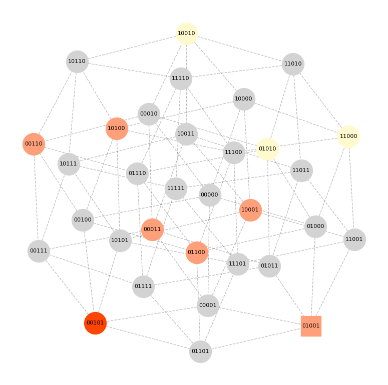
Figure 1: Solution space visualization: Current FTR center {0,0,1,0,1} (red), FTR solutions (orange), other feasible solutions (yellow), infeasible solutions (gray). Optimal solution {0,1,0,0,1} (square marker). Dashed edges indicate Hamming distance = 1.

The algorithm initializes with three random configurations: $\boldsymbol{x}_{1}=\{1,0,1,0,0\}$, $\boldsymbol{x}_{2}=\{0,0,1,0,1\}$ and $\boldsymbol{x}_{3}=\{0,0,1,1,0\}$. Evaluating these solutions using the spatial hypercube model yields $f(\boldsymbol{x}_{1})=6.31$, $f(\boldsymbol{x}_{2})=5.28$, $f(\boldsymbol{x}_{3})=7.45$. These solutions train an initial Gaussian process $GP_{global}$, which identifies $\boldsymbol{x}^{c}=\{0,0,1,0,1\}$ as the FTR center based on the lowest LCB value (visualized in Figure 1).

The adaptive swapping search then explores the FTR:

• Iteration 1: $\boldsymbol{x}_{4}=\{1,0,0,0,1\}$ (EI=0.08) yields $f=4.71$

• Iteration 2: $\boldsymbol{x}_{5}=\{0,1,0,0,1\}$ (EI=0.19) achieves the optimum $f^{*}=4.15$

Subsequent iterations confirm optimality through three consecutive failures ($n_{s}=3$), triggering a restart mechanism that updates $GP_{global}$ and identifies new FTRs until exhausting the evaluation budget $T$.

5.5 Theoretical Results

In the following theorem, we show that under a specified dispatch policy, our method converges to the optimum OPT_R within a finite number of iterations.

Theorem 9.

Let $\mathcal{S}$ be the set of feasible solutions to the $p$-MRT problem, and let $f:\mathcal{S}\rightarrow\mathbb{R}$ be the corresponding objective function. Let $\{\boldsymbol{x}_{t}\}$ be a sequence of solutions generated by our algorithm, and define $g_{t}=\min_{k\leq t}f(\boldsymbol{x}_{k})$. Then, for all $t$, we have $\boldsymbol{x}_{t}\in\mathcal{S}$, and $\lim_{t\rightarrow\infty}g_{t}=\text{OPT}_{R}$. Additionally, the algorithm converges in a finite number of iterations.

We provide a detailed proof of Theorem 9 in §D.5 in the E-Companion. In summary, we establish the convergence of Theorem 9 by demonstrating that the edge-length of the FTR will always be reduced by the design of our algorithm, leading to a restart for every FTR explored. This guarantees that the algorithm will not get contained in any local optima. Then, we prove optimality using the monotone convergence theorem (Bibby, 1974) because $g_{t}$ is monotonically non-increasing and bounded.

It is also important to show that our algorithm converges rapidly because the search space is large. Let $r_{v}=f(\boldsymbol{x}_{v}^{*})-\text{OPT}_{R}$ denote the regret for the $v$-th restart, where $\boldsymbol{x}_{v}^{*}$ is the optimum in the FTR at the $v$-th restart.

Theorem 10.

Define $\bar{r}_{V}=\frac{1}{V}\sum_{v}^{V}r_{v}$ as the average regret up to the $V$-th restart. Assume that a sample function from the Gaussian process model defined by the kernel function $k$ passes through all local optima of $f$. Then, for any $\delta\in(0,1)$, we have

$$\operatorname{Pr}\left\{\bar{r}_{V}\leq\sqrt{8C\beta_{V}\kappa_{V}/V}\right\}\geq 1-\delta,$$ (21)

where $\beta_{V}=2\log(\pi^{2}V^{2}{N\choose p}/6\delta)$, $\kappa_{V}=\mathcal{O}(2^{N}\log V)$, and $C=1/\log\left(1+\sigma^{-2}\right)$.

We present the proof of Theorem 10 in §D.6. The regret bound states that, with high probability, the average regret is bounded by a sublinear function of the number of restarts. This bound is derived from the properties of GP, the designed kernel function, and the LCB acquisition function.

6 Numerical Experiments

This section presents systematic numerical evaluations of our approaches, including: (i) SparBL: Implementation of Algorithm 2; (ii) GP-$p$M: Implementation of Algorithm 4 with $p$-Median prior mean function; (iii) GP-zero: Implementation of Algorithm 4 with zero mean function, as a special case of GP-$p$M. We compare against the following established benchmarks: (i) classical $p$-Median algorithm; (ii) BOCS (Bayesian Optimization of Combinatorial Structures) (Baptista & Poloczek, 2018); (iii) Genetic algorithm (GA) for emergency deployment (Geroliminis et al., 2011).

The simulation environment consists of a $10\times 10$ grid ($M=100$ subregions) with randomly sampled facility locations with detailed experimental setup specified in§ C.1.

As demonstrated in Figure 2, our SparBL and GP-$p$M algorithms consistently achieve optimal solutions across all configurations. For small-scale problems (Fig 2. a–b), both methods perfectly match the globally optimal solutions obtained through exhaustive enumeration. In medium and large-scale problems (Fig 2. c–f), our approaches maintain their optimal performance while significantly outperforming traditional methods. Specifically, SparBL and GP-$p$M converge to solutions that are 23–31% better than the $p$-Median baseline and 12–18% superior to GA results, with the performance gap widening as problem size increases. Notably, in the most challenging configuration ($N=50,p=30$), our methods successfully navigate the enormous search space and converge within 120 iterations, while $p$-Median, GA and BOCS become trapped in suboptimal solutions. The consistent optimality of SparBL and GP-$p$M across all test cases demonstrates their robustness and scalability, particularly in high-dimensional optimization scenarios where traditional methods fail to explore the solution space effectively.

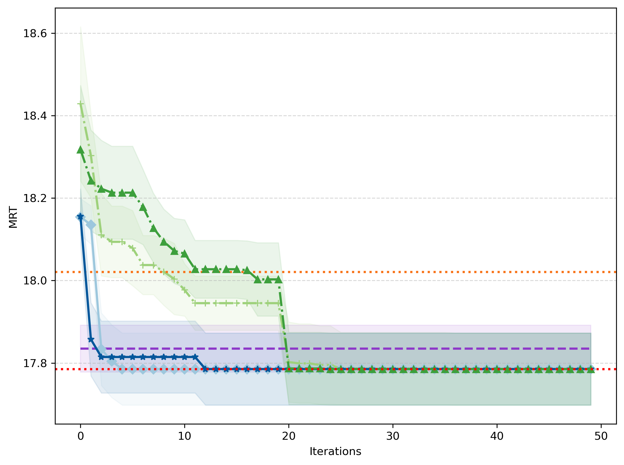
(a) $N=10,\ p=5$

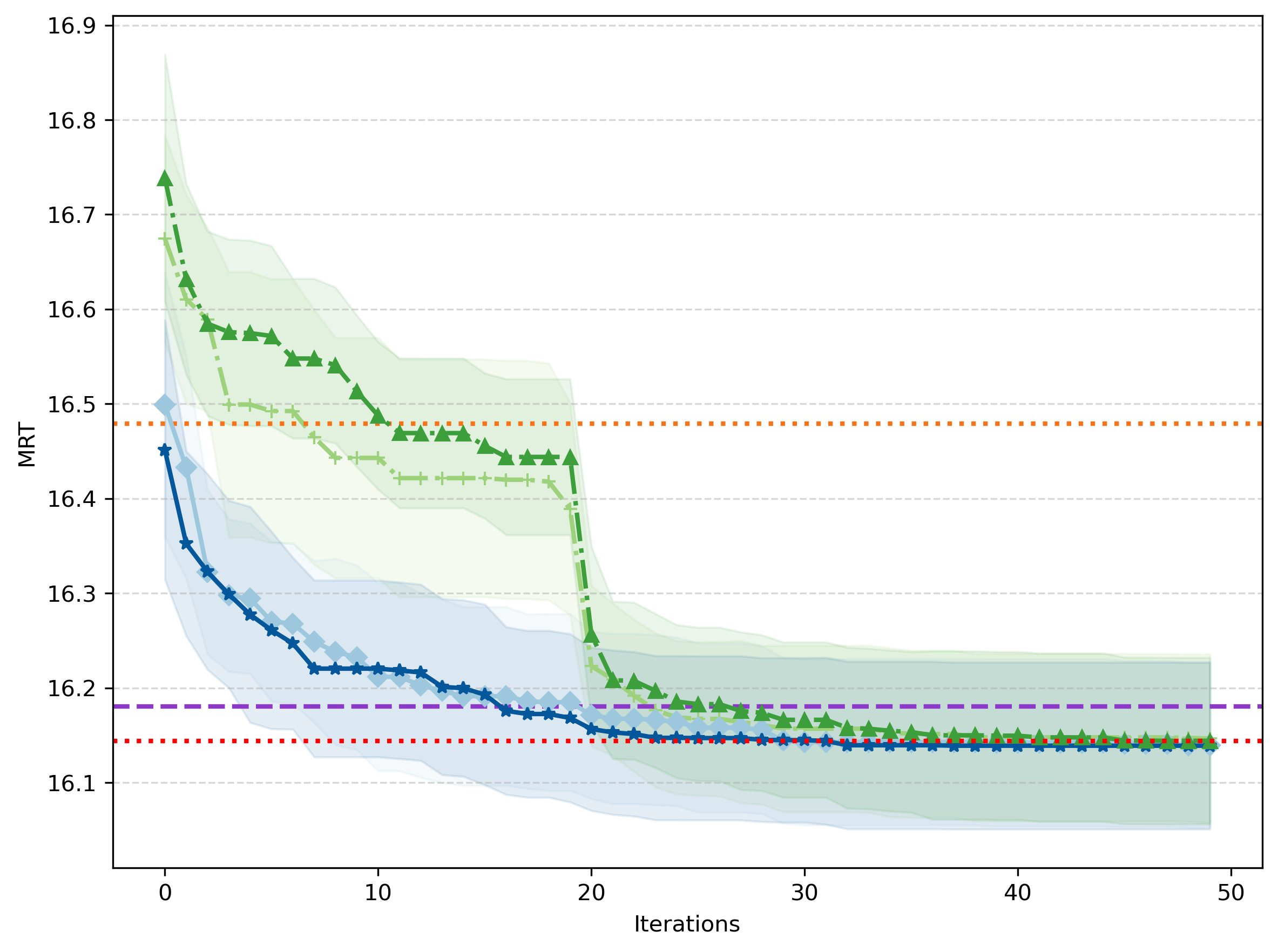
(b) $N=20,\ p=10$

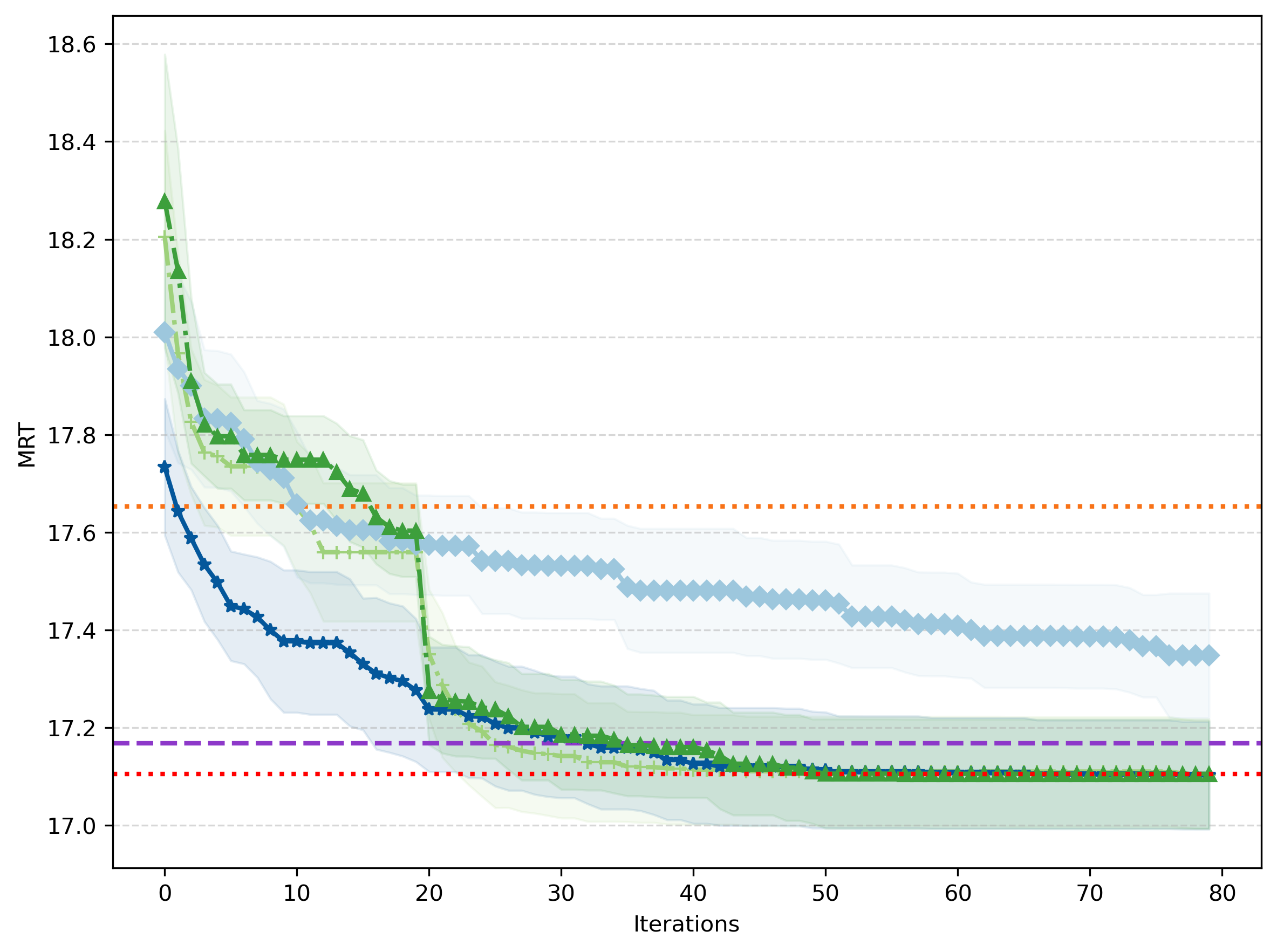
(c) $N=30,\ p=5$

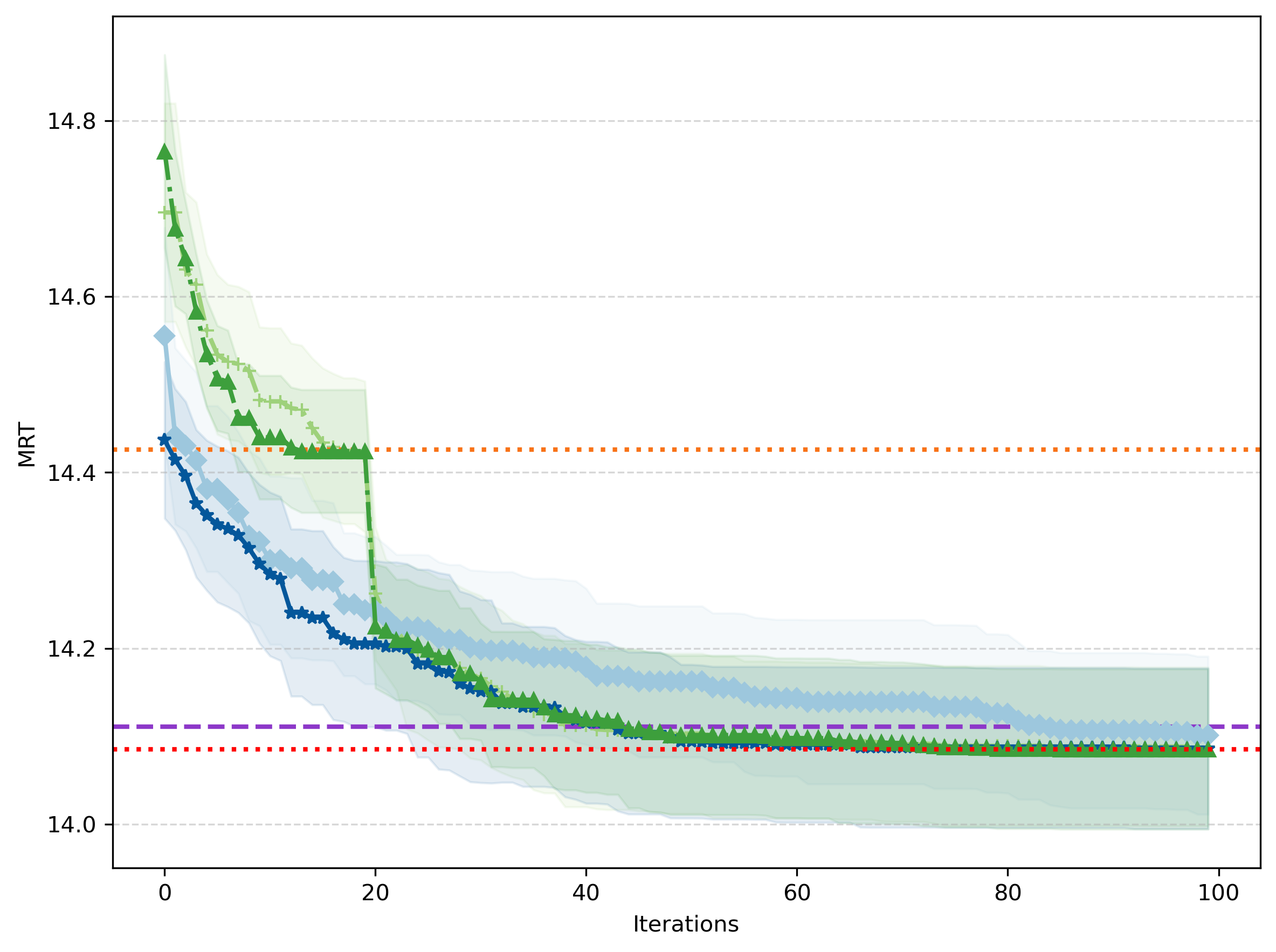
(d) $N=30,\ p=15$

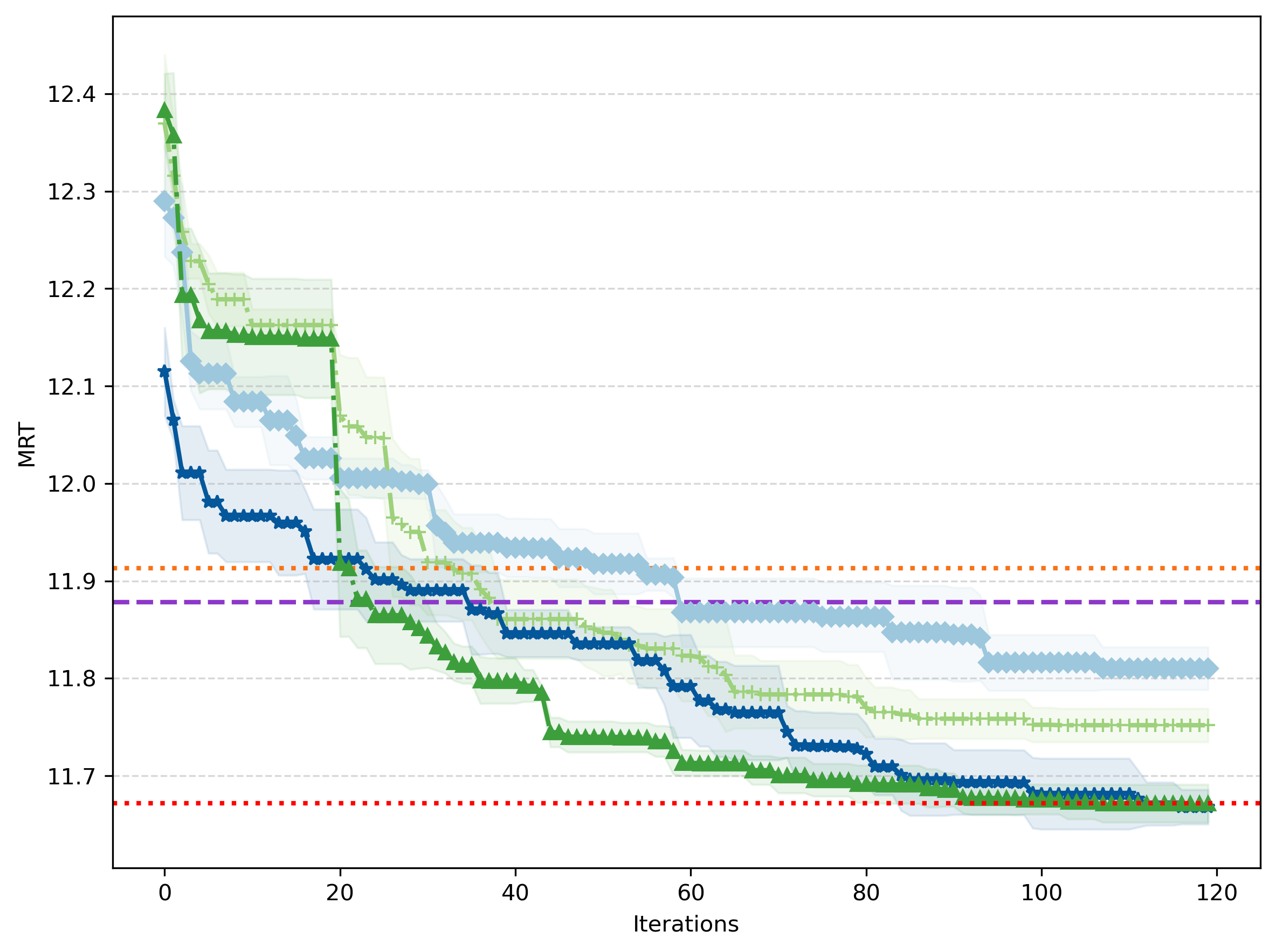
(e) $N=50,\ p=20$

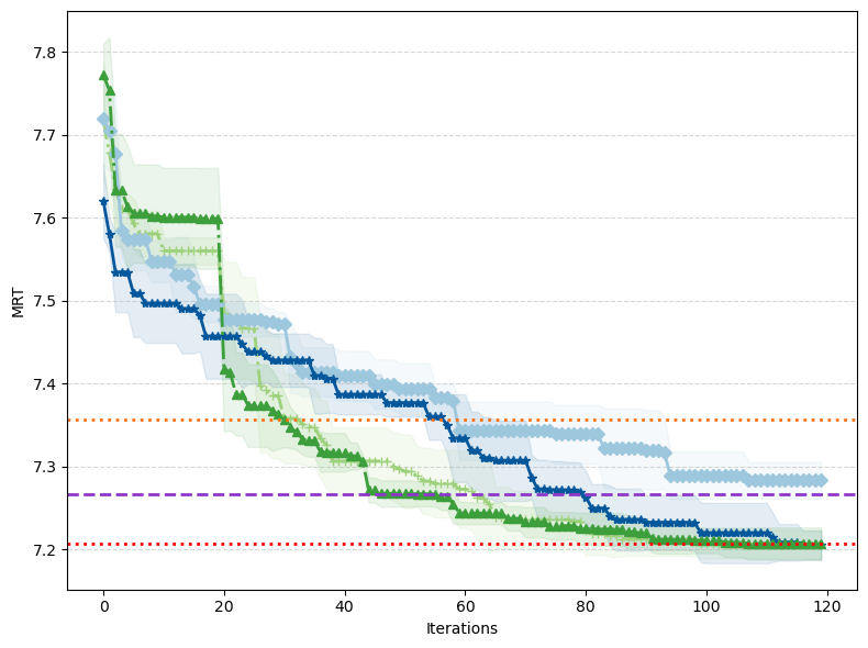
(f) $N=50,\ p=30$

Figure 2: Numerical comparison of different algorithms under varying parameter configurations. For $p$-Median and GA, we only report the final value.

In some experiments, we observe a cusp point at iteration 20, after which there is a noticeable decrease in the mean response time. This is because the initial exploration period of our algorithm was set to $\mathcal{T}=20$. After completing the initial exploration period, these 20 collected solutions were input to the BO algorithm. Our algorithm learns the structure of the problem from the information collected during the exploration phase and quickly identifies solutions with a greater chance of reducing the objective function value.

7 An Ambulance Location Case Using St. Paul, MN, Data

Based on 2020 census data, St. Paul has a population of 311,527. Our study utilizes 2014 emergency medical call records containing ambulance locations and incident reports (total 30,911 cases), with each call’s arrival time and nearest street intersection recorded. All data were anonymized to comply with HIPAA regulations. The ambulance location optimization problem positions 9 ambulances among 17 candidate stations (Figure 3) to minimize average response time.

Figure 3: St. Paul, MN map showing the 17 available station locations.

Fire Department reports indicate a uniform turnout time of 1.75 minutes across all stations for medical calls, though our methodology in § 3 accommodates location-dependent variations. We aggregated demand by partitioning the city into 71 census tract regions, calculating travel times from each tract centroid to candidate stations via Google Maps API. This spatial discretization enables efficient optimization while maintaining geographic fidelity.

7.1 Performance of Our Bayesian Optimization Approaches

Our analysis confirms that both SparBL and GP-$p$M consistently achieve optimal solutions in all experimental configurations. For brevity, we primarily present GP-$p$M results in subsequent visualizations.

Figure 5 demonstrates the ambulance deployment solution obtained by GP-$p$M, where station locations are marked by solid squares. Through exhaustive enumeration of all $\binom{17}{9}=24,\!310$ possible configurations, we verify that our method identifies the globally optimal deployment — achieving the minimal system-wide average response time of 5.86 minutes within just 80 iterations. The spatial distribution of response times reveals expected geographical patterns: centrally located tracts and those proximate to ambulance stations exhibit faster response times, while peripheral areas experience longer delays. We also evaluated the differences in ambulance locations between the $p$-Median solution and the optimal solution. Our finding shows that the $p$-Median solution has fewer units in the city center. We present the details of the $p$-Median result and its comparison to our solution in §C.2. This spatial variation validates the geographical sensitivity of our optimization framework.

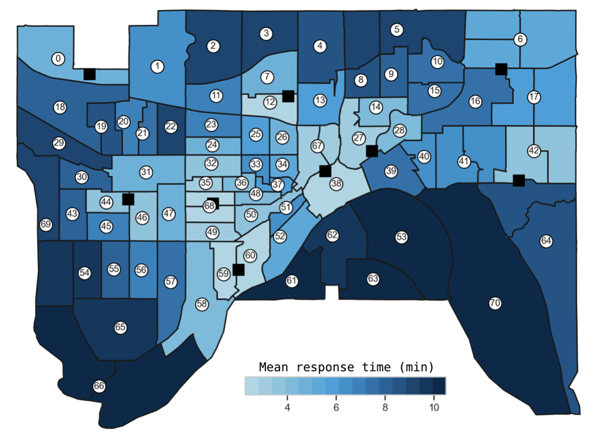
Figure 4: BO solutions for St. Paul displaying ambulance locations (solid squares) and census tracts (numbered circles 0–70). Color intensity represents mean response times across subregions, with darker shades indicating longer response durations.

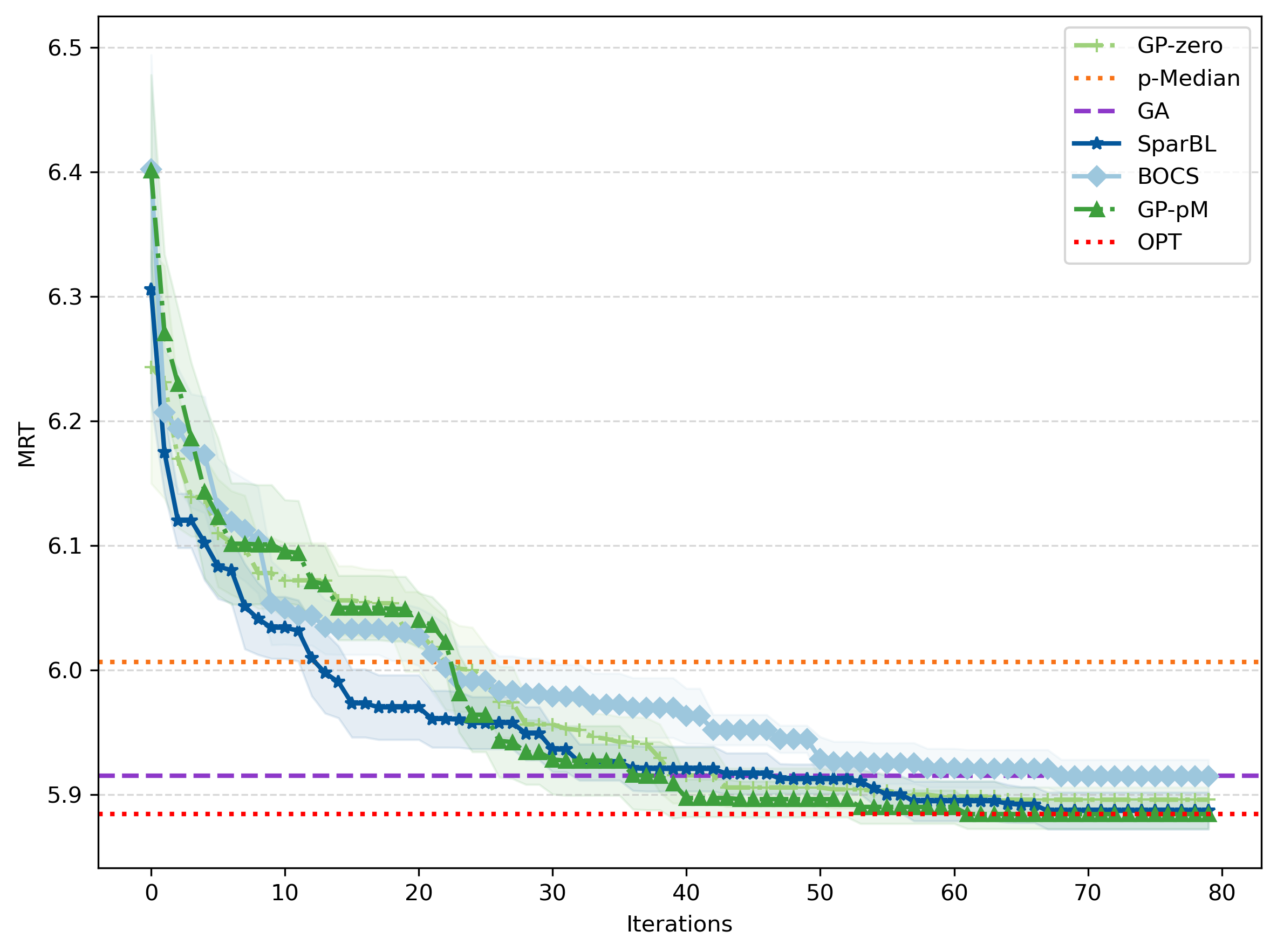
Figure 5: Performance comparison of our proposed algorithms versus baselines for St. Paul, showing convergence over optimization iterations. Results represent the mean and 95% confidence interval across 10 independent runs.

As shown in Figure 5, our methods consistently converge to the optimal solution within 80 iterations across all trials. This represents a significant computational improvement over exhaustive enumeration, reducing number of evaluations from 24,310 to fewer than 100 — a nearly 99% reduction in solution space exploration while maintaining guaranteed optimality. The rapid convergence demonstrates our framework’s efficiency in navigating large combinatorial spaces characteristic of urban emergency response optimization.

7.2 Impact of Increased Arrival Rates on Optimal Unit Locations

In this section, We further tested the solutions under varying traffic load. Compared with Figure 5, Figure 7 demonstrates that when arrival rates double, our solution strategically repositions two units toward the city center: the unit originally located at the intersection of tracts 53 and 62 relocates to central tract 12, while the tract 9 unit moves to the high-demand junction of tracts 27, 28, and 39. These spatial adjustments reveal an important operational insight - higher demand intensities necessitate centralized deployment in urban cores while maintaining distributed coverage in peripheral areas. The results empirically validate that our BO approach automatically identifies and implements this demand-responsive positioning strategy.

Table 1 demonstrates that with increasing arrival rates, our approaches consistently find the optimal solution, while the $p$-Median solution deteriorates. This supports the argument that the $p$-Median approach is suitable for low-traffic scenarios but performs less well in high-traffic environments, while our Bayesian optimization approach finds the optimal solution even in high-traffic conditions.

Table 1: Performance comparison at varying arrival rates $\lambda$. The number with an asterisk represents the original arrival rate.

Offered Load	Opt (min)	SparBL	GP-$p$M	$p$-Median	Gap ($p$-Median vs. Opt)	Gap (SparBL/GP-$p$M vs. Opt)
0.1	5.54	5.54	5.54	5.55	0.01	0.00
$0.225^{*}$	5.86	5.86	5.86	6.01	0.15	0.00
0.3	6.11	6.11	6.11	6.27	0.16	0.00
0.4	6.51	6.51	6.51	6.70	0.19	0.00
0.5	6.93	6.93	6.93	7.17	0.24	0.00
0.6	7.27	7.27	7.27	7.58	0.31	0.00
0.7	7.61	7.61	7.61	8.03	0.42	0.00
0.8	7.90	7.90	7.90	8.41	0.51	0.00
0.9	8.15	8.15	8.15	8.74	0.59	0.00
1.0	8.34	8.34	8.34	9.01	0.67	0.00

Many U.S. cities have higher ambulance utilization rates than St. Paul. In such cities, our BO approaches outperform the $p$-Median model, with the performance gap widening as utilization increases. These methods are particularly valuable in high-utilization settings, where traditional models struggle to provide optimal solutions.

Table 2 presents estimated ambulance utilizations across U.S. cities, derived from the 2019 Firehouse Magazine survey (pre-pandemic to avoid COVID-19 distortions). We excluded cities without survey responses or clear ambulance counts on official websites. Utilization rates were approximated using St. Paul’s average service rate, though actual rates in high-demand cities are likely even higher due to longer service times. This table highlights how our methods gain an increasing advantage over the $p$-Median approach as utilization rises.

Table 2: Utilization of EMS units in different regions and cities.

City	Yearly Med Calls	Calls per Minute	# of Ambulances	Utilization
New York	2,128,560	4.05	450	30.6%
Chicago	596,807	1.14	80	48.3%
Baltimore	183,306	0.35	27	43.9%
Philadelphia	272,772	0.52	57	30.9%
Los Angeles	414,375	0.79	148	18.1%
Phoenix	194,406	0.37	36	34.9%
Washington DC	173,004	0.33	38	29.5%
San Antonio	164,458	0.31	40	26.9%
Las Vegas	89,728	0.17	24	24.5%
Boston	143,189	0.27	26	36.1%
Nashville	82,221	0.16	28	19.3%
Tampa	74,634	0.14	18	27.2%
St. Louis	71,439	0.14	10	46.8%
Milwaukee	70,461	0.13	12	38.5%
Memphis	125,144	0.24	32	25.6%
Albuquerque	96,421	0.18	20	31.6%
St. Paul	30,911	0.07	9	22.5%

London, UK, is a city where our approach would be useful because its average ambulance utilization is extremely high.  Bavafa & Jónasson (2023) and Bavafa & Jónasson (2021) studied the London ambulance system, examining the effects of worker fatigue and experience on ambulance service times, using an extensive data set of calls over a 10-year period. We learned from the authors that the average ambulance utilization in their dataset was about 84%. A study of the London system would use our model to find locations to minimize average response time, while examining additions to the number of ambulances in the system aimed at reducing average response time.

7.3 Bounds Evaluation

In this section, we aim to assess the lower and upper bounds for the optimal solution derived in Section 3.2. Specifically, we fix all other parameters in the St. Paul example and vary the service rates of units, and then perform a numerical evaluation of the bounds to determine how tight they are. Table 3 displays the results of this analysis, showing the upper and lower bounds for various service rates, as well as the optimal values obtained by enumerating all possible solutions. In the St. Paul analysis, we use $\mu=42$ or 42 calls served per day, which is equivalent to an average of about 34 minutes per call.

Table 3: Numerical results of lower and upper bounds for different service rates. Number with asterisk represent the original service rate.

$\mu$	Opt (min)	GP-$p$M	SparBL	Lower Bound (min)	Upper Bound (min)
10	8.25	8.25	8.25	5.33	8.88
15	7.39	7.39	7.39	5.33	7.74
20	6.83	6.83	6.83	5.33	6.98
25	6.43	6.43	6.43	5.33	6.53
30	6.17	6.17	6.17	5.33	6.26
$42^{*}$	5.86	5.86	5.86	5.33	5.92
50	5.76	5.76	5.76	5.33	5.80
100	5.54	5.54	5.54	5.33	5.54
150	5.47	5.47	5.47	5.33	5.47
200	5.43	5.43	5.43	5.33	5.43
300	5.40	5.40	5.40	5.33	5.40
500	5.37	5.37	5.37	5.33	5.37
1000	5.35	5.35	5.35	5.33	5.35

As service rates increase, the difference between the upper and lower bounds decreases, and the upper bound gradually approaches the optimal value. We derive the lower bound from the $p$-Median problem, which is independent of the service rate and is tight when the service rate is high, as shown in the table, when the lower bound is close to the optimal value as the service rate increases. The upper bound is relatively tight. Additionally, our solutions yield the optimal solution for all service rates.

7.4 An Alternative Objective Function: Fraction of Responses over a Time Threshold

Beyond average response time, a critical EMS performance metric is the fraction of calls exceeding a response time threshold (Blackwell & Kaufman, 2002; Ingolfsson et al., 2008; Nasrollahzadeh et al., 2018). We therefore reformulate our optimization problem to minimize this fraction:

$$\min_{\boldsymbol{x}}\sum_{i\in I}\sum_{j\in J}\mathbbm{1}\{\tau_{i}+t_{ij}\geq\bar{T}\}q_{ij}(\boldsymbol{x}),$$ (22)

where $\bar{T}$ represents the response time threshold, and $q_{ij}(\boldsymbol{x})$ is the service allocation probability from (1c).

Our approach demonstrates significant advantages over traditional methods, as shown in Figure 7. At an 8-minute threshold, GP-$p$M and SparBL achieve a 7.83% late-response rate compared to the $p$-Median’s 10.8% (38.5% higher). This performance gap widens to 50% at a 9-minute threshold (3.88% vs. 5.76%).

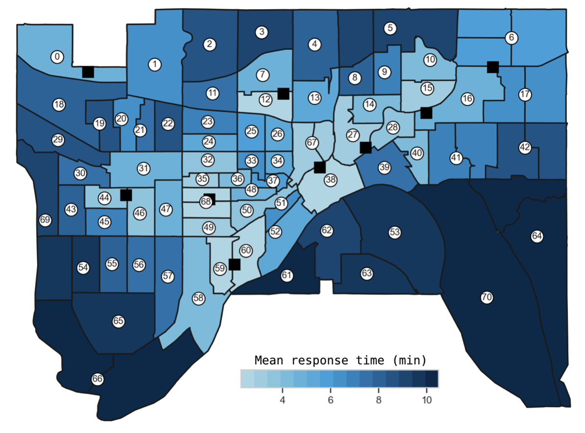
Figure 6: Two times the original arrival rate: Unit locations obtained from GP-$p$M.

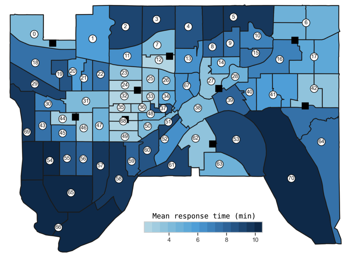
Figure 7: Alternative objective function: Unit locations for the 7-minute threshold

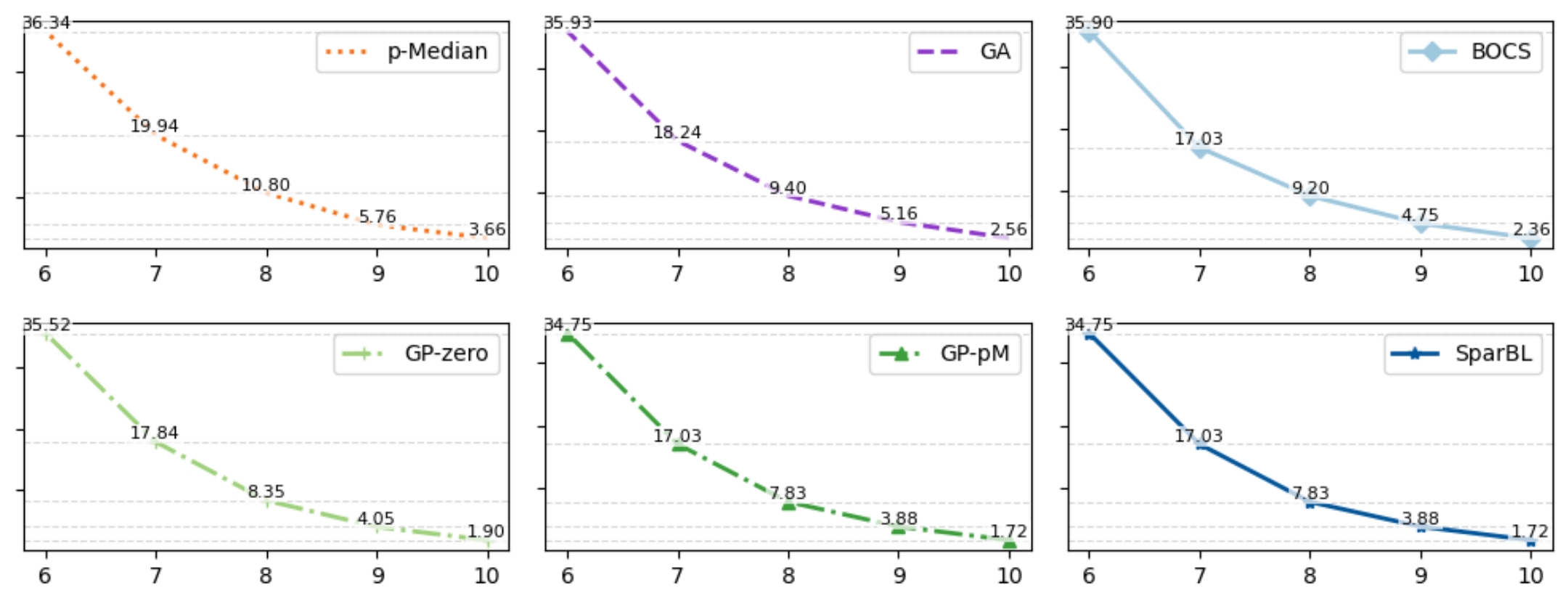
Figure 8: Alternative objective: Percentage (%) of calls exceeding time thresholds.

Figure 8 demonstrates the spatial configuration generated by our method when optimizing for a 7-minute response time threshold, contrasting sharply with the average-time-optimal layout in Figure 7. The threshold-based solution exhibits two strategic relocations: (i) the tract 59-60 border unit shifts outward to tract 62, and (ii) the central tract 38-67 hub unit disperses northeastward to tract 24. These movements reflect a systematic rebalancing from demand-centric clustering to coverage-oriented dispersion. While average-time minimization aggregates units near high-call-density zones, threshold optimization induces more geographically equitable distributions to mitigate long-tail response delays. This fundamental trade-off between efficiency and equity in EMS deployment is further quantified for an 8-minute threshold in §C.3.

8 Conclusion

In this paper, we addressed the NP-hard problem of optimizing server locations in stochastic emergency service systems by developing two novel Bayesian optimization approaches: (i) a parametric method leveraging sparse Bayesian linear regression with horseshoe priors (SparBL), and (ii) a non-parametric method combining Gaussian processes with $p$-Median priors (GP-$p$M). We derived theoretical lower and upper bounds for the optimal solution and proved that both algorithms achieve sublinear regret, with SparBL demonstrating superior scalability in high-dimensional settings.

Our numerical experiments and case study using real-world data from the St. Paul Fire Department demonstrated that both methods consistently outperform traditional $p$-Median solutions, particularly under high unit utilization. The $p$-Median approach, while effective in low-utilization scenarios, fails to account for system stochasticity, leading to degraded performance as call rates increase. In contrast, our Bayesian optimization framework adapts to these dynamics, with its relative advantage growing as utilization rises — a critical feature for real-world deployment in busy urban systems.

To guide practical implementation, we identified high-utilization cities where our approach offers the most significant benefits. Future work will extend this framework to jointly optimize dispatching policies and location decisions. These results establish our model as a rigorous and scalable tool for emergency service planning, bridging the gap between theoretical guarantees and operational needs in large-scale systems.

SUPPLEMENTARY MATERIAL of
“Optimizing Server Locations for Stochastic Emergency Service Systems”

Appendix A Illustration of BO in a Simple Continuous Example

Bayesian optimization is an approach that is particularly useful for problems where the objective function is expensive or time-consuming to evaluate, or for which the gradient is not available (Frazier 2018b). It is based on the idea of building a surrogate model of the objective function, and using a so-called acquisition function based on the surrogate model to determine the next solution to be evaluated.

Figure 9 illustrates the basic idea of BO using a simple one-dimensional example, where solution points are evaluated and added sequentially at each iteration. This illustration optimizes in a continuous space, in contrast to optimizing in a combinatorial space, which is more challenging.

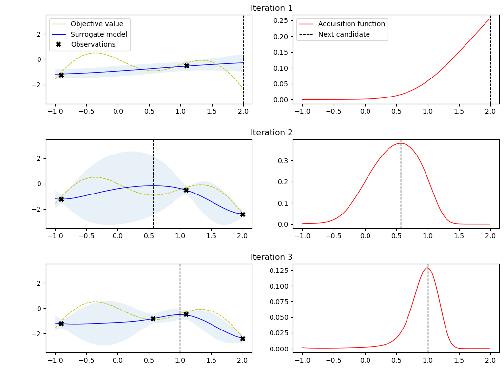
Figure 9: A simple illustration of the Bayesian optimization framework in a one-dimensional continuous space.

The left-hand side of the figure shows three subplots that illustrate the evolution of the surrogate model as solutions are observed and added to the model. The locations of the observed solutions are indicated by the $\times$ symbol. In the first iteration, we randomly select two solutions that are added to the model. In each subsequent iteration, the algorithm selects the solution with the highest acquisition function value for evaluation, shown by the dashed vertical lines. The plots show how the surrogate model is updated based on the newly observed solutions. The right-hand side of the figure shows three subplots that demonstrate the role of the acquisition function. The acquisition function provides a trade-off between exploration (sampling new solutions with high predicted variances) and exploitation (sampling solutions with high predicted means). Typically, the points with high mean values and high variances have higher values for the acquisition functions, as shown in the three subplots on the left.

An Overview of Our BO Approaches

The location problem consists of locating $p$ units at $N$ candidate locations. The optimal solution, denoted by $\boldsymbol{x^{*}}$, is a vector of 0s and 1s, where 1 means a unit is at location $i$ and 0 means location $i$ is empty. The optimal objective value, denoted by $f(\boldsymbol{x^{*}})$, is a real number representing the mean response time.

The main idea of our approach is to evaluate each potential solution $\boldsymbol{x}$ in turn and use the resulting $f(\boldsymbol{x})$ to identify the next solution to evaluate. Throughout the paper, evaluating a solution refers to computing the value of the objective function in the $p$-MRT problem of (1a).

Initially, we randomly choose $\mathcal{T}$ solutions $\boldsymbol{x}_{1},\cdots,\boldsymbol{x}_{\mathcal{T}}$, and evaluate $f(\boldsymbol{x}_{1}),\cdots,f(\boldsymbol{x}_{\mathcal{T}})$. We use these solutions and their evaluations to train a surrogate model. We then use an acquisition function to identify the next solution $\boldsymbol{x}_{\mathcal{T}+1}$. We then evaluate $f(\boldsymbol{x}_{\mathcal{T}+1})$, and update the surrogate model. We continue the process until we reach an evaluation budget of $T$. The final solution is the solution with the lowest objective function value among all evaluated solutions.

Appendix B Spatial Hypercube Approximation

The objective function value of a given solution $\boldsymbol{x}$, which is $f(\boldsymbol{x})=\sum_{j\in J}(\tau_{i}+t_{ij})q_{ij}(\boldsymbol{x})$, must be evaluated at each step. Computing this exactly requires solving the spatial hypercube model introduced by Larson (1974), which becomes computationally prohibitive for large-scale instances. To address this, we adopt the approximation algorithm proposed by Larson (1975), which provides an efficient method for estimating the mean response time. The key idea is to first assume that servers are statistically independent, treating each as either busy or idle, regardless of the state of others. Under this assumption, the system reduces to an Erlang loss model, which yields closed-form expressions for the distribution of the number of busy servers. To improve accuracy, the method introduces a correction factor $Q$, which adjusts for the dependencies between server states. This approximation framework has been extended to accommodate general service time distributions (Jarvis 1985), systems with multiple units per station (Budge et al. 2009), and cross-trained service units (Hua & Swersey 2022), further enhancing its applicability to realistic emergency service environments.

Define $p_{ijk}$ as the probability that unit $i$ is dispatched as the $k$-th preferred unit at node $j$. Unit $i$ will be dispatched only if it is available and all $k-1$ units more preferred are busy.

$$p_{ijk}=\operatorname{Pr}\left[W_{i}^{c}\cap\left\{\bigcap_{l=1}^{k-1}W_{\gamma_{jl}}\right\}\right],$$ (23)

where $W_{i}$ is the event that unit $i$ is busy, $W^{c}_{i}$ is the event that unit $i$ is available, and $\gamma_{jl}$ is the index of the $l$-th preferred unit in subregion $j$ in the preference list.

Recall that the rate at which calls arrive at node $j$ is $\lambda_{j}$. Then, the rate at which unit $i$ is dispatched to node $j$ as the $k$-th preferred unit is $\lambda_{j}p_{ijk}$, and the rate, $S_{i}$, at which unit $i$ is dispatched to calls from all demand nodes is

$$S_{i}=\sum_{j\in G_{i}^{1}}\lambda_{j}p_{ij1}+\sum_{j\in G_{i}^{2}}\lambda_{j}p_{ij2}+\cdots+\sum_{j\in G_{i}^{N}}\lambda_{j}p_{ijN}=\sum_{k=1}^{N}\sum_{j\in G_{i}^{k}}\lambda_{j}p_{ijk},$$ (24)

where $G_{i}^{k}$ is defined as the set of nodes for which unit $i$ is the $k$-th preferred unit. Specifically, $G_{i}^{k}=\{j\in\{1,\cdots,J\}:\gamma_{jk}=i\}$. $S_{i}$ can also be expressed as the product of the utilization of unit $i$ and the service rate of unit $i$ , i.e.,

$$S_{i}=\rho_{i}\mu_{i}.$$ (25)

Larson (1975) developed an approximation for $p_{ijk}$ by first assuming server independence and then applying a correction factor to correct for dependence. We have

$$p_{ijk}\approx Q(N,\bar{\rho},k-1)\prod_{l=1}^{k-1}\rho_{\gamma_{jl}}(1-\rho_{i}),$$ (26)

where $Q(N,\bar{\rho},\cdot)$ is a correction factor for server dependence and $\bar{\rho}=\frac{\lambda}{N\mu}(1-P_{b})$ is the average utilization of all units, where $P_{b}$ is the blocking probability that all units are busy. Define $P(k)$ as the probability that exactly $k$ servers are busy. The correction factor is given by

$$Q(N,\bar{\rho},r)=\sum_{k=r}^{N-1}\frac{{k\choose r}}{{N\choose r}}\frac{N-k}{N-r}\frac{P(k)}{\bar{\rho}^{r}(1-\bar{\rho})}.$$ (27)

The probabilities $P(k)$ and $P_{b}=P(N)$ are obtained by the Erlang loss formula.

Now, we have all the components needed to estimate $\rho_{i}$. Denote the estimated unit utilization by $\widehat{\rho}_{i}$. Using (24), (25), and (26), we have

$$\widehat{\rho}_{i}=\frac{S_{i}}{\mu_{i}}=\frac{1}{\mu_{i}}\sum_{k=1}^{N}\sum_{j\in G_{i}^{k}}\lambda_{j}p_{ijk}=\frac{1}{\mu_{i}}\sum_{k=1}^{N}\sum_{j\in G_{i}^{k}}\lambda_{j}Q(N,\bar{\rho},k-1)\prod_{l=1}^{k-1}\widehat{\rho}_{\gamma_{jl}}(1-\widehat{\rho}_{i}),$$ (28)

where we obtain $Q(N,\bar{\rho},k)$ from (27). Dividing both sides of (28) by $1-\widehat{\rho}_{i}$ and collecting terms of $\widehat{\rho}_{i}$, we approximate the unit utilizations by the following $N$ non-linear equations,

$$\widehat{\rho}_{i}=1-\Big{(}1+\frac{1}{\mu_{i}}\sum_{k=1}^{N}\sum_{j\in G_{i}^{1,k}}\lambda_{j}Q(N,\bar{\rho},k)\prod_{l=1}^{k-1}\widehat{\rho}_{\gamma_{jl}}\Big{)}^{-1},\qquad i=1,2,\cdots,N$$ (29)

We solve these $N$ non-linear equations iteratively to obtain $\widehat{\rho}_{i}$. In contrast, the exact set of locations requires solving $2^{N}$ detailed balance equations. The hypercube approximation algorithm provides an estimate $\widehat{q}_{ij}$. We have

$$\widehat{q}_{ij}=\left\{\begin{array}[]{ll}\frac{\lambda_{j}}{\sum_{j}\lambda_{j}}\left(1-\widehat{\rho}_{i}\right),&\qquad i=\gamma_{j1},\\ \frac{\lambda_{j}}{\sum_{j}\lambda_{j}}Q(N,\bar{\rho},k-1)\left(\prod_{l=1}^{k-1}\widehat{\rho}_{\gamma_{jl}}\right)\left(1-\widehat{\rho}_{i}\right),&\qquad i=\gamma_{jk},\forall k\geq 2.\end{array}\right.$$ (30)

In Figure 10, we show that the approximation is very close to the exact value, with a mean absolute error of less than 0.002 minutes, obtained by generating 100 random setups for small (15 units), median (20 units), and large problems (30 units). For a system with 30 units, the approximation algorithm takes less than 0.01 seconds while the exact solution requires solving $2^{30}$ simultaneous equations which takes hours.

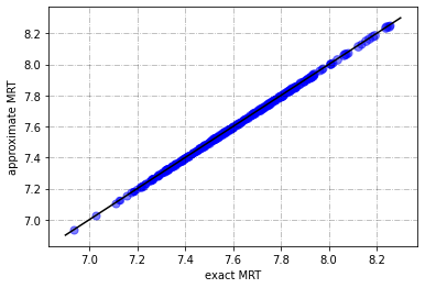
(a) Exact MRT vs. Approximate MRT

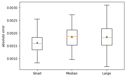
(b) Box-plots of absolute errors

Figure 10: The accuracy of the spatial hypercube approximation algorithm.

Appendix C Further Examination of the St. Paul Case Study Results

C.1 Experiment Setup

For GP-based methods, we initialize with edge length $d_{0}=20$ and set hyperparameters as follows: $n_{s}=3$, $n_{f}=10$, $\alpha_{s}=1.5$, $\alpha_{f}=2/3$, and $\beta=25$. All experiments were conducted on an Apple M1 system with 16GB RAM, with consistent hyperparameters across both simulation experiments and the case study in Section 7.

C.2 Analysis of the $p$-median Solution

Figure 12 displays the configuration found by the $p$-median solution. We compare it to Figure 4 in the main text, which shows the optimal unit locations found by the Bayesian optimization when the objective is to minimize average response time. The $p$-median solution produced a mean response time of 5.92 minutes, which is higher than the optimal value of 5.86 minutes.

Compared to the optimal solution, the $p$-median solution moves two units. One unit moves from the intersection of tracts 27, 28, and 39 to tract 62, and the other moves from the intersection of tracts 7 and 12 to tract 9. The units move away from the city center, as the $p$-median solution assumes all units are always available and the single unit at the center can handle the large number of calls.

This relocation results in longer response times for tracts 2, 3, 4, 7, 11, 12, and 13, all at the top of the city map, and for all tracts in the city center. This is due to the increased utilization of the centrally located unit. The $p$-median solution performs better at the city periphery but negatively impacts response time near the city center, which would be even worse in large cities with high population densities in the city center. In St. Paul, MN, although the population is dispersed, the center still has the highest concentration. Hence, the $p$-median solution does not yield the optimal result.

C.3 Response Times Beyond the Time Threshold

Figure 12 displays the unit locations determined by our Bayesian optimization approach when the time threshold is set to 8 minutes. We compare this figure to Figure 7 in the main text, which represents the optimal unit locations based on average response time.

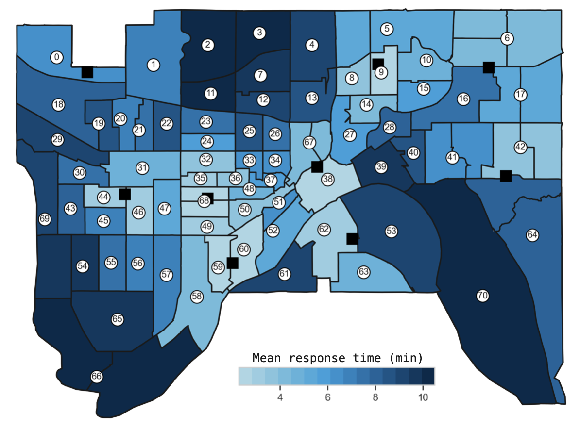
Figure 11: Unit locations from the $p$-median approach.

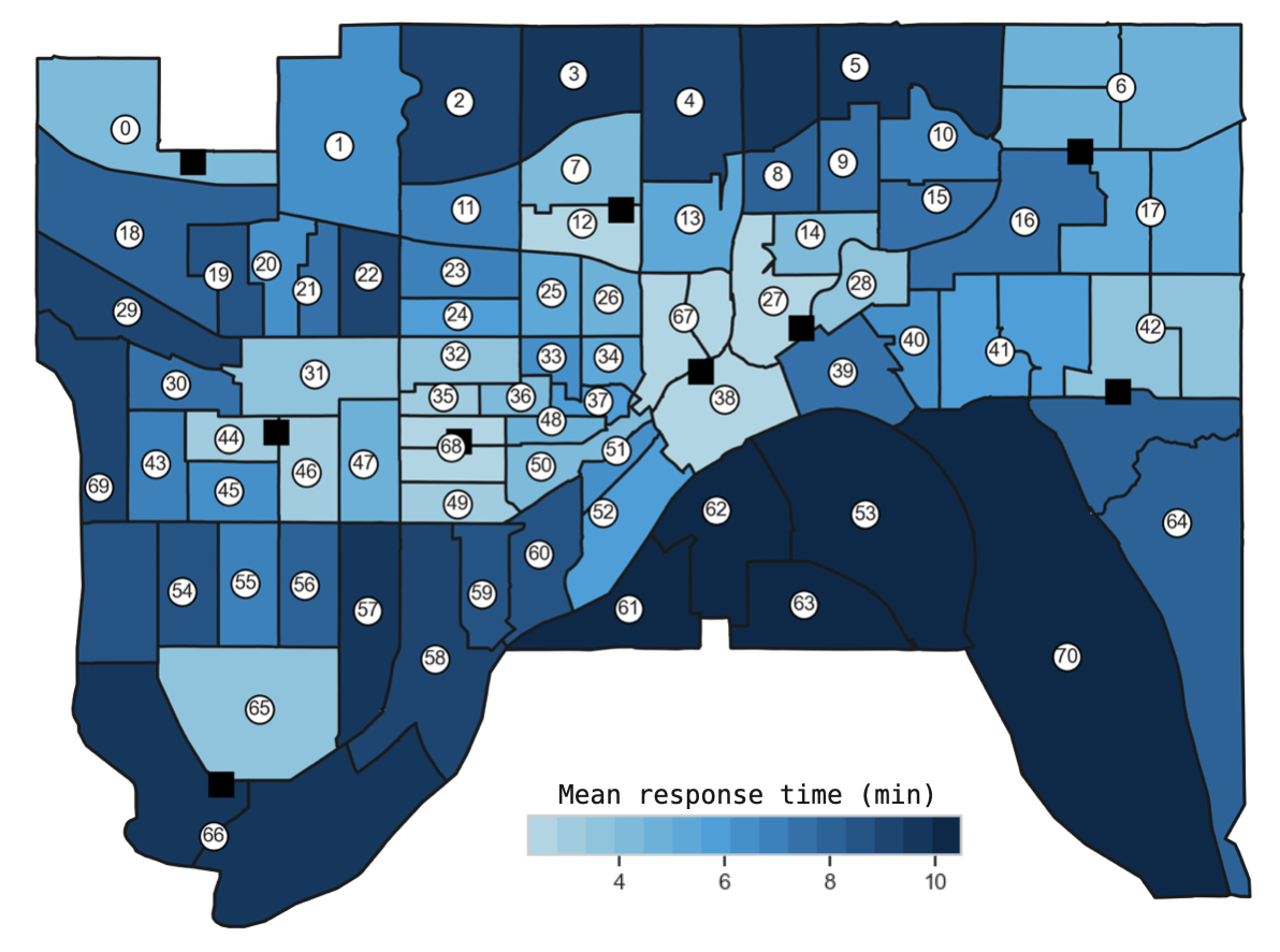
Figure 12: Unit locations for the 8-minute response time threshold.

In this configuration, one unit moves compared to the optimal arrangement. Specifically, the unit previously located at the junction of tracts 59 and 60 moves to tract 66 in the lower left area. This shift enables the unit at tract 68 to serve tracts 59, 60, 61, and nearby regions within the 8-minute response time. The relocated unit at tract 66 now satisfies the 8-minute threshold requirement for tracts in the lower left region of the city.

Compared to Figure 7 in the main text, where the time threshold is 7 minutes, there is a notable change with the unit at the intersection of tracts 53, 62, and 63 moved back to the city center. This adjustment was made because these tracts, along with other adjacent ones, are now within an 8-minute travel distance from the unit in the city center. As a result, the revised time threshold of 8 minutes is now satisfied without the need for a dedicated unit in that region.

Appendix D Miscellaneous Proofs

D.1 Proof of Theorem 1

Proof.

Proof.

We prove that the $p$-MRT problem is NP-hard by a polynomial reduction of the $p$-median problem, which is known to be NP-hard (Kariv & Hakimi 1979).

In the $p$-MRT problem, recall that $\lambda_{j}$ is the call arrival rate from subregion $j$, $P(\boldsymbol{b})$ is the probability of being in state $\boldsymbol{b}$, and $\Pi_{j}$ is the probability that all units that can serve sub-region $j$ are busy. We define the weight of subregion $j$, $w_{j}$, as the normalized arrival rate $\lambda_{j}/\sum_{k\in J}\lambda_{k}$, and $q_{ij}(\boldsymbol{x})$ is the fraction of calls in subregion $j$ that are responded to by the unit at location $i$ given unit configuration $\boldsymbol{x}$, as given by

$$q_{ij}(\boldsymbol{x})=\frac{\sum_{\boldsymbol{b}\in S_{ij}(\boldsymbol{x})}\lambda_{j}P(\boldsymbol{b})}{\sum_{k\in J}\lambda_{k}\left(1-\Pi_{j}\right)}=w_{j}\frac{\sum_{\boldsymbol{b}\in S_{ij}(\boldsymbol{x})}P(\boldsymbol{b})}{1-\Pi_{j}}.$$ (31)

Given an instance $\mathcal{I}$ of the $p$-median problem, we construct an instance $\mathcal{I}^{\prime}$ of the $p$-MRT problem by setting $S_{ij}(\boldsymbol{x})$ in $\mathcal{I}^{\prime}$ such that

$$\frac{\sum_{\boldsymbol{b}\in S_{ij}(\boldsymbol{x})}P(\boldsymbol{b})}{1-\Pi_{j}}=y_{ij}.$$ (32)

In $\mathcal{I}^{\prime}$, the set $S_{ij}(\boldsymbol{x})$ denotes states where the unit at location $i$ is designated for calls from subregion $j$. We observe that a significant challenge is the binary assignment requirement of the $p$-median, which dictates that each sub-region $j$ be assigned exclusively to one location $i$. Conversely, the $p$-MRT model does not inherently impose such constraints. To address this, we establish the assignment rule for the $p$-MRT problem as follows: if $y_{ij}=1$ in $\mathcal{I}$, then in $\mathcal{I}^{\prime}$, assign unit $i$ as the primary responder and the sole unit to cover sub-region $j$. Should unit $i$ be occupied, any incoming calls from sub-region $j$ are disregarded. Furthermore, we assign $S_{ij}(\boldsymbol{x})=\varnothing$ for all $i$ and $j$ pairs in $\mathcal{I}^{\prime}$ where $y_{ij}=0$ in $\mathcal{I}$.

Consequently, for $y_{ij}=0$ in $\mathcal{I}$, $\sum_{\boldsymbol{b}\in S_{ij}(\boldsymbol{x})}P(\boldsymbol{b})=0$ in $\mathcal{I}^{\prime}$. Additionally, for $y_{ij}=1$ in $\mathcal{I}$, we derive

$$\frac{\sum_{\boldsymbol{b}\in S_{ij}(\boldsymbol{x})}P(\boldsymbol{b})}{1-\Pi_{j}}=\frac{1-\rho_{i}}{1-\Pi_{j}}=1.$$ (33)

The first equality arises because, when each sub-region $j$ is assigned exclusively to one location $i$, then $S_{ij}(\boldsymbol{x})$ represents the set of states where the unit at location $i$ is available. Therefore, summing over the probabilities of all such states, $\sum_{\boldsymbol{b}\in S_{ij}(\boldsymbol{x})}P(\boldsymbol{b})$, equates to the probability that the unit at location $i$ is available, which is $1-\rho_{i}$, with $\rho_{i}$ representing the unit’s utilization. The second equality is valid because the fraction of calls from sub-region $j$ that are blocked, $\Pi_{j}$, equals the probability that the unit at location $i$ is busy, $\rho_{i}$, when the unit from location $i$ exclusively serves sub-region $j$.

Consequently, (32) holds, and all constraints in the $p$-median problem are met through such an equivalence relationship. By this construction, we ensure that a solution to $\mathcal{I}$ corresponds to a solution to $\mathcal{I}^{\prime}$ and vice versa. Consequently, if we solve $\mathcal{I}^{\prime}$ optimally, we obtain an optimal solution to $\mathcal{I}$ as well, thus proving the reduction from the $p$-median problem to the $p$-MRT problem in polynomial time. Since the $p$-median problem is already known to be NP-hard, we conclude that the $p$-MRT problem is also NP-hard. $\square$

∎

D.2 Proof of Theorem 2

Proof.

Proof.

We prove this theorem by first showing that the feasible region of $p$-MRT is a subset of the feasible region of the $p$-median problem, and the optimal value of the $p$-median problem (denoted by $\text{OPT}_{M}$) is a lower bound to the optimal value of the $p$-MRT problem (denoted by $\text{OPT}_{R}$). Let $\widetilde{y}_{ij}=\sum_{\boldsymbol{b}\in S_{ij}(\boldsymbol{x})}P(\boldsymbol{b})/(1-\Pi)$, where $\Pi$ is the probability that all units are busy, also known as the blocking probability. We first show that $\sum_{i\in I}\widetilde{y}_{ij}=1$ for all $j\in J$.

Recall that $S_{ij}(\boldsymbol{x})$ is the set of states in which the unit at location $i$ is assigned to calls from subregion $j$ given the set of unit locations $\boldsymbol{x}$. Thus, $\boldsymbol{b}\in S_{ij}(\boldsymbol{x})$ indicates that in state $\boldsymbol{b}$, unit $i$ is the first preferred available unit. Let $\boldsymbol{B}$ denote the set of all possible states given the set of unit locations $\boldsymbol{x}$. The cardinality of $\boldsymbol{B}$ is $|\boldsymbol{B}|=2^{p}$. We have

$$\widetilde{y}_{ij} =\frac{\sum_{\boldsymbol{b}\in S_{ij}(\boldsymbol{x})}P(\boldsymbol{b})}{1-\Pi}=\frac{\sum_{\boldsymbol{b}\in\boldsymbol{B}}P(\boldsymbol{b})\mathbbm{1}_{\{\boldsymbol{b}\in S_{ij}(\boldsymbol{x})\}}}{1-\Pi}=\frac{\sum_{\boldsymbol{b}\in\boldsymbol{B}}P(\boldsymbol{b})\mathbbm{1}_{\{b_{i}=0\}}\prod_{k<\eta_{j}(i)}\mathbbm{1}_{\{b_{\gamma_{jk}}=1\}}}{1-\Pi},$$

where $\gamma_{jl}$ is the index of the $l$-th preferred unit in subregion $j$ in the preference list, and $\eta_{j}(i)$ is the preference rank of unit $i$ in subregion $j$. In the last line of the above equation, $\prod_{k<\eta_{j}(i)}\mathbbm{1}_{\{b_{\gamma_{jk}}=1\}}$ indicates whether all units with preference ranks higher than unit $i$ are busy in state $\boldsymbol{b}$..

Let $X_{ij}^{\boldsymbol{b}}=\sum_{i\in I}\mathbbm{1}_{\{b_{i}=0\}}\prod_{k<\eta_{j}(i)}\mathbbm{1}_{\{b_{\gamma_{jk}}=1\}}$. We have

$$\sum_{i\in I}\widetilde{y}_{ij} =\sum_{i\in I}\frac{\sum_{\boldsymbol{b}\in\boldsymbol{B}}P(\boldsymbol{b})\mathbbm{1}_{\{b_{i}=0\}}\prod_{k<\eta_{j}(i)}\mathbbm{1}_{\{b_{\gamma_{jk}}=1\}}}{1-\Pi}$$

$$=\frac{\sum_{\boldsymbol{b}\in\boldsymbol{B}}P(\boldsymbol{b})\sum_{i\in I}\mathbbm{1}_{\{b_{i}=0\}}\prod_{k<\eta_{j}(i)}\mathbbm{1}_{\{b_{\gamma_{jk}}=1\}}}{1-\Pi}=\frac{\sum_{\boldsymbol{b}\in\boldsymbol{B}}P(\boldsymbol{b})X_{ij}^{\boldsymbol{b}}}{1-\Pi}.$$

Denote $\boldsymbol{b}^{*}$ as the state where all units are busy. We first claim that $X_{ij}^{\boldsymbol{b}^{*}}=0$, which follows directly from the fact that $b_{i}=1$ for all $i$ in state $\boldsymbol{b}^{*}$, and $\mathbbm{1}_{\{b_{i}=0\}}=0$ for all $i$.

We next show that $X_{ij}^{\boldsymbol{b}}=1$ for all $\boldsymbol{b}\in\boldsymbol{B}\setminus\boldsymbol{b}^{*}$. Denote by $\mathscr{G}_{j}^{l}$ the set of states in which the $l-1$ most preferred units are busy and the $l$-th preferred unit is available in subregion $j$. We have

$$\mathscr{G}_{j}^{l}=\{\boldsymbol{b}:b_{\gamma_{jl}}=0,b_{\gamma_{jk}}=1,\ \forall k<l,\boldsymbol{b}\in\boldsymbol{B}\}.$$ (34)

We claim that

$$\cup_{l=1}^{N}\mathscr{G}_{j}^{l}\cup\{\boldsymbol{b}^{*}\}=\boldsymbol{B},\qquad\forall j\in J,$$ (35)

since all states except for $\boldsymbol{b}^{*}$ belong to $\cup_{l=1}^{N}\mathscr{G}_{j}^{l}$ by construction of the set $\mathscr{G}_{j}^{l}$.

For all states in which the most preferred unit is available, i.e., $\forall\boldsymbol{b}\in\mathscr{G}_{j}^{1}$, we have

$$X_{ij}^{\boldsymbol{b}} =\mathbbm{1}_{\{b_{\gamma_{j1}}=0\}}+\sum_{i\not=\gamma_{j1}}\mathbbm{1}_{\{b_{i}=0\}}\prod_{k<\eta_{j}(i)}\mathbbm{1}_{\{b_{\gamma_{jk}}=1\}}=1+\sum_{i\not=\gamma_{j1}}\mathbbm{1}_{\{b_{i}=0\}}\mathbbm{1}_{\{b_{\gamma_{j1}}=1\}}\prod_{1<k<\eta_{j}(i)}\mathbbm{1}_{\{b_{\gamma_{jk}}=1\}}=1,$$

since $\forall\boldsymbol{b}\in\mathscr{G}_{j}^{1}$ we have $\mathbbm{1}_{\{b_{\gamma_{j1}}=0\}}=1$ and $\mathbbm{1}_{\{b_{\gamma_{j1}}=1\}}=0$ because $\gamma_{j1}$ is the most preferred free unit in subregion $j$.

For all states in which the $l-1$ most preferred units are busy and the $l$-th preferred unit is available, i.e., $\forall\boldsymbol{b}\in\mathscr{G}_{j}^{l}$ and $j>1$, we have

$$X_{ij}^{\boldsymbol{b}} =\sum_{i:\eta_{j}(i)<l}\mathbbm{1}_{\{b_{i}=0\}}\prod_{k<\eta_{j}(i)}\mathbbm{1}_{\{b_{\gamma_{jk}}=1\}}+\mathbbm{1}_{\{b_{\gamma_{jl}}=0\}}\prod_{k<l}\mathbbm{1}_{\{b_{\gamma_{jk}}=1\}}+\sum_{i:\eta_{j}(i)>l}\mathbbm{1}_{\{b_{i}=0\}}\prod_{k<\eta_{j}(i)}\mathbbm{1}_{\{b_{\gamma_{jk}}=1\}}$$

$$=1+\sum_{i:\eta_{j}(i)>l}\mathbbm{1}_{\{b_{i}=0\}}\bigg{(}\prod_{k<l}\mathbbm{1}_{\{b_{\gamma_{jk}}=1\}}\bigg{)}\mathbbm{1}_{\{b_{\gamma_{jl}}=1\}}\bigg{(}\prod_{l<k<\eta_{j}(i)}\mathbbm{1}_{\{b_{\gamma_{jk}}=1\}}\bigg{)}=1,$$

since $\forall\boldsymbol{b}\in\mathscr{G}_{j}^{l}$ we have $\mathbbm{1}_{\{b_{\gamma_{jl}}=0\}}=1$ and $\mathbbm{1}_{\{b_{\gamma_{jl}}=1\}}=0$ by definition, and $\mathbbm{1}_{\{b_{i}=0\}}=0$ for $\eta_{j}(i)<l$ and $\prod_{k<l}\mathbbm{1}_{\{b_{\gamma_{jk}}=1\}}=1$.

Combining the above equations, we have

$$\sum_{i\in I}\widetilde{y}_{ij} =\frac{\sum_{\boldsymbol{b}\in\boldsymbol{B}}P(\boldsymbol{b})X_{ij}^{\boldsymbol{b}}}{1-\Pi}=\frac{\sum_{\boldsymbol{b}\in\boldsymbol{B}\setminus\boldsymbol{b}^{*}}P(\boldsymbol{b})X_{ij}^{\boldsymbol{b}}+\Pi\cdot X_{ij}^{\boldsymbol{b}^{*}}}{1-\Pi}=\frac{1-\Pi}{1-\Pi}=1.$$

We obtain equation (D.2) because $X_{ij}^{\boldsymbol{b}}=1$ for $\boldsymbol{b}\in\boldsymbol{B}\setminus\boldsymbol{b}^{*}$, $X_{ij}^{\boldsymbol{b}^{*}}=0$, and $\sum_{\boldsymbol{b}\in B}P(\boldsymbol{b})=1$.

Thus, we have demonstrated that $\sum_{i\in I}\widetilde{y}_{ij}=1$ for all $j\in J$, fulfilling Constraint (5c) of the $p$-median problem, while the $p$-MRT problem inherently satisfies Constraint (5b). We further argue that Constraint (5d) is met. This is because, for $x_{i}=0$, indicating no unit at location $i$, $S_{ij}=\emptyset$ leads to $\widetilde{y}_{ij}=0$. For $x_{i}=1$, given that $\sum_{i\in I}\widetilde{y}_{ij}=1$ and each $\widetilde{y}_{ij}$ is non-negative by definition, Constraint (5d) is met. Additionally, by defining $w_{j}=\lambda_{j}/\sum_{k\in J}\lambda_{k}$, we align the objective function of the $p$-MRT problem with that of the $p$-median.

With this transformation and any specified dispatch policy, the $p$-MRT simplifies to the following:

$$\text{OPT}_{R}=\min_{\boldsymbol{x},\boldsymbol{y}} \sum_{i\in I}\sum_{j\in J}w_{j}(\tau_{i}+t_{ij})\widetilde{y}_{ij}$$ (36)

s.t. $$\sum_{i\in I}x_{i}=p,$$ (37)

$$\sum_{i\in I}\widetilde{y}_{ij}=1,\forall j\in J,$$ (38)

$$\widetilde{y}_{ij}\leq x_{i},\forall i\in I,\forall j\in J,$$ (39)

$$x_{i}\in\{0,1\},\forall i\in I$$ (40)

where $\widetilde{y}_{ij}=\sum_{\boldsymbol{b}\in S_{ij}(\boldsymbol{x})}P(\boldsymbol{b})/(1-\Pi)\in[0,1]$ is fixed and determined by the solution $\boldsymbol{x}=\{x_{1},\cdots,x_{N}\}$ and the assignment rule.

Next, we show that $\text{OPT}R\geq\text{OPT}M$ always holds. To prove this, we argue that for any feasible solution $\boldsymbol{x}={x_{1},\ldots,x_{N}}$ (including the optimal solution for the $p$-MRT problem), we have

$$\sum_{i\in I}w_{j}(\tau_{i}+t_{ij})y^{*}_{ij}\leq\sum_{i\in I}w_{j}(\tau_{i}+t_{ij})\widetilde{y}_{ij},$$ (41)

where $y^{*}_{ij}$ is the optimal solution to the $p$-median problem given $\boldsymbol{x}$. The basic idea is to show that for each sub-region $j\in J$, we have

$$\sum_{i\in I}w_{j}(\tau_{i}+t_{ij})y^{*}_{ij}=\min_{i:x_{i}=1}w_{j}(\tau_{i}+t_{ij}),$$ (42)

and

$$\sum_{i\in I}w_{j}(\tau_{i}+t_{ij})\widetilde{y}_{ij}\geq\min_{i:x_{i}=1}w_{j}(\tau_{i}+t_{ij}).$$ (43)

To see (42) holds, we note that we set no constraint on $y_{ij}$ across sub-regions $j$ when $x_{i}=1$. Thus, for each sub-region $j\in J$, the optimal value is attained at the minimum value of $w_{j}(\tau_{i}+t_{ij})$. For (43), we have

$$\sum_{i\in I}w_{j}(\tau_{i}+t_{ij})\widetilde{y}_{ij}\geq\sum_{i\in I}\widetilde{y}_{ij}\big{(}\min_{i:x_{i}=1}w_{j}(\tau_{i}+t_{ij})\big{)}=\min_{i:x_{i}=1}w_{j}(\tau_{i}+t_{ij}).$$ (44)

Thus, we conclude that for any feasible solution $\boldsymbol{x}=\{x_{1},\cdots,x_{N}\}$ of $p$-MRT, the optimal value for the $p$-median problem is no larger than that for the $p$-MRT problem. Therefore, the optimal value of the $p$-median problem is a lower bound on the optimal value of the $p$-MRT problem, i.e.,

$$\text{OPT}_{R}\geq\text{OPT}_{M}.$$ (45)

$\square$∎

D.3 Proof of Theorem 6

The key technical tool used in our regret analysis is the posterior contraction property in high-dimensional Bayesian linear regression. In particular, we invoke Proposition 11 to control the $\ell_{1}$-distance between the posterior sample $\widehat{\alpha}_{t}$ and he true parameter $\alpha$ at each time step $t\in[T]$.

The argument proceeds in three stages. First, we establish sparsity recovery by bounding the posterior mass on overly complex models, leveraging the horseshoe’s exponential tail decay properties. Second, we control prediction error through the compatibility condition and the prior’s concentration around sparse vectors. Finally, we convert these results into $\ell_{1}$-norm estimation error bounds using the effective sparsity induced by the prior’s shrinkage behavior.

Consider the probability space for the sparse linear model using horseshoe priors. Let $\alpha$ denote the true parameter vector. The bandit environment generates context-reward pairs ($\boldsymbol{x}_{t},y_{t}$), where the contexts are drawn from arm-specific distributions and may depend on the history of actions. The joint distribution $\mathcal{Q}_{t}$ over $\left(\alpha,\boldsymbol{x}_{t},y_{t}\right)$ is defined by combining the horseshoe prior with the data-generating process

$$\alpha\mid\beta_{k},\tau,\sigma\sim\mathcal{N}(0,\beta_{k}^{2}\tau^{2}\sigma^{2}),\qquad(X_{t},y_{t})\mid\alpha\sim\text{HS}_{t}(\alpha,\tau,\mathcal{P}_{\epsilon}).$$

where $\mathrm{HS}_{t}$ denotes the horseshoe prior of contexts and rewards at time $t$ given $\alpha$, $\beta_{k}$ and $\tau$ are local and global hypervariances, and the noise distribution $\mathcal{P}_{\epsilon}$, as given in (7).

Proposition 11 (Posterior Contraction with Horseshoe Prior).

Under Assumptions 4 and 5, for the horseshoe prior with global shrinkage parameter $\tau\asymp\frac{s_{0}}{D}$, the posterior satisfies:

$$\mathbb{E}_{\mathcal{D}_{t}}\left(\|\alpha-\widehat{\alpha}_{t}\|_{1}\geq C\sigma Ws_{0}\sqrt{\frac{\log D}{t}}\;\Big{|}\;{\mathcal{D}_{t}}\right)\lesssim D^{-s_{0}}+2t^{-1},$$

where $\mathcal{G}_{t}=\{\phi_{\text{comp}}(s_{0};X_{t})\geq\phi_{0}\}$ and $\mathcal{N}_{t}=\{\max_{j}|\epsilon_{t}^{\top}X_{t}^{(j)}|\leq W\sigma\sqrt{2t(\log D+\log t)}\}$.

Proof.

Proof. We first establish a bound on the mean squared error of the posterior mean estimate.

Lemma 12.

Under Assumptions 4 and 5, the horseshoe posterior mean $\widehat{\alpha}_{t}$ satisfies:

$$\sup_{\alpha\in\ell_{0}[s_{0}]}\mathbb{E}\|\alpha-\widehat{\alpha}_{t}\|_{2}^{2}\lesssim\frac{s_{0}\log D}{t}+(D-s_{0})\tau\sqrt{\log\frac{1}{\tau}}.$$

With the choice $\tau\asymp\frac{s_{0}}{D}$, this becomes:

$$\mathbb{E}\|\alpha-\widehat{\alpha}_{t}\|_{2}^{2}\lesssim\frac{s_{0}\log D}{t}.$$

Proof.

Proof. Let $\widetilde{s}_{0}=\#\{j:\alpha_{j}\neq 0\}\leq s_{0}$, and without loss of generality, let $\alpha_{j}\neq 0$ for $j=1,\ldots,\widetilde{s}_{0}$ and $\alpha_{j}=0$ for $j=\widetilde{s}_{0}+1,\ldots,D$. We decompose the mean squared error:

$$\mathbb{E}\|\widehat{\alpha}_{t}-\alpha\|_{2}^{2}=\sum_{j=1}^{\widetilde{s}_{0}}\mathbb{E}_{\alpha_{j}}(\widehat{\alpha}_{t,j}-\alpha_{j})^{2}+\sum_{j=\widetilde{s}_{0}+1}^{D}\mathbb{E}_{0}\widehat{\alpha}_{t,j}^{2}.$$ (46)

We proceed by bounding the two terms separately. First, we present two lemmas from van der Pas et al. 2014.

Lemma 13.

For $\tau^{2}<1$, the absolute value of the difference between the horseshoe estimator $\widehat{\alpha}$ and an observation $\widetilde{\alpha}$ can be bounded by a function $h(\widetilde{\alpha},\tau)$ such that for any $c>2$:

$$\lim_{\tau\downarrow 0}\sup_{|\widetilde{\alpha}|>\sqrt{c\sigma^{2}\log\frac{1}{\tau}}}h(\widetilde{\alpha},\tau)=0.$$

Lemma 14.

If $\tau^{2}<1$, the posterior mean of the horseshoe prior can be bounded above by:

$$\widehat{\alpha}\leq\widetilde{\alpha}e^{\frac{\widetilde{\alpha}^{2}}{2\sigma^{2}}}f(\tau),$$

where $f$ is such that $f(\tau)\leq\frac{2}{3}\tau$.

(i). To bound the first terms in (46), for active indices ($j\leq\widetilde{s}_{0}$), define the threshold $\zeta_{\tau}=\sqrt{2\sigma^{2}\log(1/\tau)}$. Decompose the squared error:

$$(\widehat{\alpha}_{t,j}-\alpha_{j})^{2}=(\widehat{\alpha}_{t,j}-\widetilde{\alpha}_{t,j}+\widetilde{\alpha}_{t,j}-\alpha_{j})^{2}\stackrel{{\scriptstyle(a)}}{{\leq}}2(\widetilde{\alpha}_{t,j}-\alpha_{j})^{2}+2(\widehat{\alpha}_{t,j}-\widetilde{\alpha}_{t,j})^{2}$$

where (a) results from $(a+b)^{2}\leq 2a^{2}+2b^{2}$.

Recall that $\varepsilon_{t}\sim\mathcal{N}(0,\sigma^{2})$, the first term satisfies

$$\mathbb{E}(\widetilde{\alpha}_{t,j}-\alpha_{j})^{2}\leq\frac{\sigma^{2}}{t},$$

which gives

$$\sum_{j=i}^{\widetilde{s}_{0}}\mathbb{E}(\widetilde{\alpha}_{t,j}-\alpha_{j})^{2}\leq\frac{\widetilde{s}_{0}\sigma^{2}}{t},$$

Using Lemma 13, the bias introduced by the horseshoe prior is bounded by

$$\sup_{y}|\widehat{\alpha}_{t,j}(\widetilde{\alpha})-\widetilde{\alpha}|\lesssim\zeta_{\tau}.$$

Thus, we have

$$\mathbb{E}_{\alpha_{j}}(\widehat{\alpha}_{t,j}-\alpha_{j})^{2}\lesssim\frac{\sigma^{2}}{t}+\zeta_{\tau}^{2}.$$ (47)

(ii). To bound the second term in (46), for inactive indices ($j>\widetilde{s}_{0}$), we split the expectation:

$$\mathbb{E}_{0}\widehat{\alpha}_{t,j}^{2}=\mathbb{E}_{0}[\widehat{\alpha}_{t,j}^{2}\mathbbm{1}_{\{|\widetilde{\alpha}_{t,j}|\leq\zeta_{\tau}\}}]+\mathbb{E}_{0}[\widehat{\alpha}_{t,j}^{2}\mathbbm{1}_{\{|\widetilde{\alpha}_{t,j}|>\zeta_{\tau}\}}].$$ (48)

For small signal region, where $|\mathbf{y}_{t,j}|\leq\zeta_{\tau}$, we have

$$\mathbb{E}_{0}[\widehat{\alpha}_{t,j}^{2}\mathbbm{1}_{\{|\widetilde{\alpha}_{t,j}|\leq\zeta_{\tau}\}}]\leq\int_{-\zeta_{\tau}}^{\zeta_{\tau}}\widetilde{\alpha}^{2}e^{\widetilde{\alpha}^{2}/\sigma^{2}}f(\tau)^{2}\phi(\widetilde{\alpha})\text{d}\widetilde{\alpha}\stackrel{{\scriptstyle(a)}}{{\lesssim}}\sigma f(\tau)^{2}\zeta_{\tau}\tau^{-1}\stackrel{{\scriptstyle(b)}}{{\lesssim}}\zeta_{\tau}\tau,$$

where (a) follows from the integral identity and (b) from $f(\tau)\leq\frac{2}{3}\tau$ in Lemma 14. $\phi(x)=\frac{1}{\sqrt{2\pi}}\exp\left(-\frac{1}{2}x^{2}\right)$ is the pdf for standard normal distribution.

For large signal region, where $|\widetilde{\alpha}_{t,j}|>\zeta_{\tau}$, from Lemma 13 we have $\left|\widehat{\alpha}_{t,j}\right|\leq|\widetilde{\alpha}_{t,j}|$. Therefore

$$\mathbb{E}_{0}[\widehat{\alpha}_{t,j}^{2}\mathbbm{1}_{\{|\widetilde{\alpha}_{t,j}|>\zeta_{\tau}\}}]\leq\mathbb{E}_{0}[\widetilde{\alpha}_{t,j}^{2}\mathbbm{1}_{\{|\mathbf{y}_{t,j}|>\zeta_{\tau}\}}]\stackrel{{\scriptstyle(a)}}{{=}}2\sigma\zeta_{\tau}\phi(\zeta_{\tau}/\sigma)\lesssim\sigma\zeta_{\tau}\tau,$$

where (a) is from Mill’s ratio for Gaussian tails.

Combining both small and large signal regions, when $\tau<e^{-\sigma^{2}/2}$, we arrive at:

$$\sum_{j=\widetilde{s}_{0}+1}^{D}\mathbb{E}_{0}\widehat{\alpha}_{t,j}^{2}\lesssim(D-\widetilde{s}_{0})\zeta_{\tau}\tau.$$ (49)

(iii). Combining (47) and (49) yields the stated result. $\square$∎

Applying Markov’s inequality to Lemma 12,

$$\Pi_{t}\left(\|\alpha-\widehat{\alpha}_{t}\|_{2}\geq\delta\mid\mathcal{D}_{t}\right)\leq\frac{s_{0}\log(D)}{\delta^{2}t}.$$ (50)

Define the effective support set:

$$\widehat{S}_{t}=\{k:\mathbb{E}[\widehat{\alpha}_{t}^{2}\mid D_{t}]>\eta_{k}\},\quad\text{where }\eta_{k}=\frac{\log D}{t},$$

which identifies coefficients with significant posterior mass, excluding noise-dominated dimensions.

Define the event where the effective support remains sparse:

$$\mathcal{E}_{t}=\{|\widehat{S}_{t}|\leq 2s_{0}\}$$

Under this event, we maintain approximate sparsity. Under $\mathcal{E}_{t}$, the error vector $v=\alpha-\widehat{\alpha}_{t}$ has $\|v\|_{0}\leq 2s_{0}$. By Assumption 5, the design matrix $X_{t}$ satisfies the compatibility condition. Applying the compatibility condition:

$$\|\alpha-\widehat{\alpha}_{t}\|_{1}\leq\frac{\sqrt{2s_{0}}\|X_{t}(\alpha-\widehat{\alpha}_{t})\|_{2}}{\sqrt{t}\phi_{0}}.$$ (51)

Following Chakraborty et al. (2023), define the noise event:

$$\mathcal{N}_{t}=\left\{\max_{1\leq j\leq D}|\epsilon_{t}^{\top}X_{t}^{(j)}|\leq W\sigma\sqrt{2t(\log D+\log t)}\right\}$$

Finally, choose $\delta=\sqrt{\frac{s_{0}\log D}{t}}$ in (50). On $\mathcal{E}_{t}\cap\mathcal{N}_{t}$,

$$\|\alpha-\widehat{\alpha}_{t}\|_{1} \lesssim\frac{\sqrt{2s_{0}}\cdot\sqrt{s_{0}\log D}}{\sqrt{t}\phi_{0}}=\frac{s_{0}\sqrt{\log D}}{\sqrt{t}\phi_{0}}.$$

The last step is about deriving the probability bounds for the bad events $\mathcal{E}_{t}^{c}$ and $\mathcal{N}_{t}^{c}$.

For the noise event complement, we begin by analyzing the maximum correlation between the noise vector $\epsilon_{t}$ and design matrix columns $X_{t}^{(j)}$. Since $\epsilon_{t}$ is Gaussian with parameter $\sigma$ and assuming the design matrix columns are normalized ($\|X_{t}^{(j)}\|_{2}\leq W$), each inner product $\epsilon_{t}^{\top}X_{t}^{(j)}$ is Gaussian with variance proxy $\sigma^{2}W^{2}$. Applying the Gaussian tail bound

$$\mathbb{P}(|\epsilon_{t}^{\top}X_{t}^{(j)}|>u)\leq 2\exp\left(-\frac{u^{2}}{2\sigma^{2}W^{2}}\right).$$

Setting $u=W\sigma\sqrt{2(\log D+\log t)}$ yields

$$\mathbb{P}(|\epsilon_{t}^{\top}X_{t}^{(j)}|>W\sigma\sqrt{2(\log D+\log t)})\leq 2\exp(-(\log D+\log t))=\frac{2}{Dt}.$$

Taking a union bound over all $D$ columns gives

$$\mathbb{P}\left(\max_{1\leq j\leq D}|\epsilon_{t}^{\top}X_{t}^{(j)}|>W\sigma\sqrt{2(\log D+\log t)}\right)\leq D\cdot\frac{2}{Dt}=\frac{2}{t}$$

Thus we obtain $\mathbb{P}(\mathcal{N}_{t}^{c})\leq 2t^{-1}$.

For the sparsity event complement, using Theorem 3 from Chakraborty et al. (2023), we directly obtain

$$\mathbb{P}(\mathcal{E}_{t}^{c})\leq D^{-s_{0}}.$$

Therefore, the total failure probability combines both bad events through the union bound

$$\mathbb{P}((\mathcal{E}_{t}\cap\mathcal{N}_{t})^{c})=\mathbb{P}(\mathcal{E}_{t}^{c}\cup\mathcal{N}_{t}^{c})\leq\mathbb{P}(\mathcal{E}_{t}^{c})+\mathbb{P}(\mathcal{N}_{t}^{c})\leq D^{-s_{0}}+2t^{-1}$$

The result follows. $\square$∎

Now we are ready to bound the regret. We decompose the cumulative regret over the time horizon $T$ into two phases

$$r_{T}=\underbrace{\sum_{t=1}^{T_{0}}\Delta_{a_{t}}(t)}_{R_{\text{init}}}+\underbrace{\sum_{t=T_{0}+1}^{T}\Delta_{a_{t}}(t)}_{R_{\text{main}}}$$ (52)

where $T_{0}$ is a threshold to be determined later, and $\Delta_{a_{t}}(t)$ denotes the instantaneous regret at time $t$.

We begin by bounding the initial phase regret $R_{\text{init}}$. Under Assumption 4, the sparsity and boundedness of $\alpha$ imply

$$R_{\text{init}}\leq WT_{0}.$$ (53)

We now turn our attention to the main phase of the regret $R_{\text{main}}$. The following lemma provides a bound on the expected instantaneous regret after the warm-up period.

Lemma 15.

For all $t>T_{0}$, the expected regret satisfies

$$\mathbb{E}[\Delta_{a_{t}}(t)]\leq Cs_{0}\sqrt{\frac{\log D}{t}}+W(2t^{-1}+D^{-s_{0}}).$$

Proof.

Proof. Define the high-probability event $\mathcal{E}_{t}$:

$$\mathcal{E}_{t}=\left\{\|\widehat{\alpha}_{t}-\alpha\|_{1}\leq Cs_{0}\sqrt{\frac{\log D}{t}}\right\}$$

Recalling Proposition 11, on the event $\mathcal{E}_{t}$, for binary variables, the deviation between the estimated and true rewards can be bounded as:

$$\Delta_{a_{t}}(t)\leq\|\boldsymbol{x}_{t}\widehat{\alpha}_{t}-\boldsymbol{x}_{t}\alpha\|_{1}\leq CWs_{0}\sqrt{\frac{\log D}{t}}$$ (54)

On the complement event $\mathcal{E}_{t}^{c}$, we bound the regret by the maximum possible difference:

$$\Delta_{a_{t}}(t)\leq W,\quad\mathbb{P}(\mathcal{E}_{t}^{c})\leq 2t^{-1}+D^{-s_{0}}$$ (55)

Combining both cases, the total expectation is bounded as

$$\mathbb{E}\left[\Delta_{a_{t}}(t)\right]\leq\mathbb{E}\left[\Delta_{a_{t}}(t)\mid\mathcal{E}_{t}\right]\cdot\operatorname{Pr}\left(\mathcal{E}_{t}\right)+\mathbb{E}\left[\Delta_{a_{t}}(t)\mid\mathcal{E}_{t}^{c}\right]\cdot\operatorname{Pr}\left(\mathcal{E}_{t}^{c}\right)$$ (56)

which yields

$$\mathbb{E}\left[\Delta_{a_{t}}(t)\right]\leq Cs_{0}\sqrt{\frac{\log D}{t}}+W\left(2t^{-1}+D^{-s_{0}}\right).$$ (57)

$\square$∎

Summing the per-period regret bound over $t\in[T_{0},T]$, we obtain

$$R_{\text{main}} \leq Cs_{0}\sum_{t=T_{0}+1}^{T}\left(\sqrt{\frac{\log D}{t}}+W\left(2t^{-1}+D^{-s_{0}}\right)\right)$$ (58)

$$\leq Cs_{0}\sqrt{\log D}\int_{T_{0}+1}^{T}\left(2t^{-1/2}+Wt^{-1}\right)\text{d}t+\mathcal{O}(1)$$

$$\leq C^{\prime}s_{0}\sqrt{\log D}\left(\sqrt{T}-\sqrt{T_{0}}\right)+W\log T$$

where $C^{\prime}$ absorbs constant factors including $C$.

Combining (53) and (58) yields the following total regret:

$$r_{T}=WT_{0}+C^{\prime}s_{0}\sqrt{\log D}\left(\sqrt{T}-\sqrt{T_{0}}\right)+W\log T$$ (59)

The cutoff time $T_{0}$ is determined by minimizing(59) w.r.t. $T_{0}$. Taking the derivative and igoring the constants terms, we have:

$$\frac{d}{dT_{0}}\left(WT_{0}-C^{\prime}Ws_{0}\sqrt{T_{0}\log D}\right)=0$$

This yields the optimal choice:

$$T_{0}=\left\lceil C^{\prime 2}s_{0}^{2}\log D\right\rceil,$$ (60)

where $C$ depends on $W,\phi_{0}$, and $\sigma$.

Combining Equations (53) and (58), and choosing $T_{0}=\left\lceil C^{\prime 2}s_{0}^{2}\log D\right\rceil$, we obtain the following bound on the cumulative regret

$$r_{T} \leq WC^{\prime 2}s_{0}^{2}\log D+WC^{\prime 2}s_{0}^{2}\sqrt{T\log D}-WC^{\prime 2}s_{0}^{2}\sqrt{T_{0}\log D}+\log T$$

$$=\mathcal{O}\left(Ws_{0}^{2}\sqrt{T\log D}+\log T\right).$$

$\square$

D.4 Proof of Lemma 8

Proof.

Proof.

We begin by proving the first part of the lemma. Recall that $H(\boldsymbol{x},\boldsymbol{x}^{\prime})=H(\boldsymbol{x},\boldsymbol{x}^{\prime})^{+}+H(\boldsymbol{x},\boldsymbol{x}^{\prime})^{-}$ and

$$H(\boldsymbol{x},\boldsymbol{x}^{\prime})^{+}=w\left(\left[\boldsymbol{x}\cap\neg\boldsymbol{x}^{\prime}\right]\right),\qquad H(\boldsymbol{x},\boldsymbol{x}^{\prime})^{-}=w\left(\left[\neg\boldsymbol{x}\cap\boldsymbol{x}^{\prime}\right]\right).$$ (61)

When $m=1$, we have by definition $\xi^{m}(\boldsymbol{x})=\xi(\boldsymbol{x})=\{x_{1},\cdots,x_{j},\cdots,x_{i},\cdots,x_{N}\}$ and $x_{i}\not=x_{j}$. Without loss of generality, let $x_{i}=1$ and $x_{j}=0$. Then, we have

$$\boldsymbol{x}\cap\neg\xi(\boldsymbol{x}) =\{x_{1},\cdots,x_{i},\cdots,x_{j},\cdots,x_{N}\}\cap\neg\{x_{1},\cdots,x_{j},\cdots,x_{i},\cdots,x_{N}\}$$ (62)

$$=\{x_{1},\cdots,x_{i},\cdots,x_{j},\cdots,x_{N}\}\cap\{\neg x_{1},\cdots,\neg x_{j},\cdots,\neg x_{i},\cdots,\neg x_{N}\}$$

$$=\{x_{1}\cap\neg x_{1},\cdots,x_{i}\cap\neg x_{j},\cdots,x_{j}\cap\neg x_{i},\cdots,x_{N}\cap\neg x_{N}\}$$

We note that $x_{k}\cap\neg x_{k}=0$ for all $k$. In addition, $x_{i}\cap\neg x_{j}=1\cap 1=1$ and $x_{j}\cap\neg x_{i}=0\cap 0=0$. Thus, we have

$$H(\boldsymbol{x},\xi(\boldsymbol{x}))^{+}=1.$$ (63)

Following the same logic, we can determine that $H(\boldsymbol{x},\xi(\boldsymbol{x}))^{-}=1,$ and $H(\boldsymbol{x},\xi(\boldsymbol{x}))=H(\boldsymbol{x},\xi(\boldsymbol{x}))^{+}+H(\boldsymbol{x},\xi(\boldsymbol{x}))^{-}=2$.

When $m\geq 2$, we first show that $H(\boldsymbol{x},\xi^{m}(\boldsymbol{x}))\leq 2\min\{p,N-p\}$ using induction. When $p\leq N/2$, we have $\min\{p,N-p\}=p$, and we show that $H(\boldsymbol{x},\xi^{m}(\boldsymbol{x}))\leq 2p$. This holds because in order to increase the Hamming distance by two, we need to swap a new unit with a new empty site. In this case, we have more empty sites than units, so the number of units $p$ becomes the bottleneck, and the maximum number of new swaps is $2p$. The same logic applies when $p>N/2$, and in this case $H(\boldsymbol{x},\xi^{m}(\boldsymbol{x}))\leq 2(N-p)$. Therefore, we must have $H(\boldsymbol{x},\xi^{m}(\boldsymbol{x}))\leq 2\min\{p,N-p\}$.

Assume that $H(\boldsymbol{x},\xi^{m}(\boldsymbol{x}))\in\llbracket 0,2\min\{m,p,N-p\}\rrbracket\cap\mathbb{N}_{2k}$, where $\llbracket a,b\rrbracket$ indicates the interval of all integers between $a$ and $b$ included and $\mathbb{N}_{2k}$ is the set of all even natural numbers. This holds for $m=2$, because $H(\boldsymbol{x},\xi^{2}(\boldsymbol{x}))\in\{0,2,4\}$. If in both steps, the same two units $x_{i}$ and $x_{j}$ are swapped, $H(\boldsymbol{x},\xi^{2}(\boldsymbol{x}))=0$; if in the second step, $x_{i}$ is swapped with another unit $x_{m}$, then $H(\boldsymbol{x},\xi^{2}(\boldsymbol{x}))=2$; if in the second step, two other units $x_{m}$ and $x_{n}$ are swapped, then $H(\boldsymbol{x},\xi^{2}(\boldsymbol{x}))=4$.

For the $m+1$-st swap, $H(\boldsymbol{x},\xi^{m+1}(\boldsymbol{x}))\in\llbracket 0,2\min\{(m+1),p,N-p\}\rrbracket\cap\mathbb{N}_{2k}$, because when two other units are swapped, the Hamming distance increases by two, as shown above. The maximum Hamming distance cannot exceed $\max\{p,N-p\}$. $\square$

D.5 Proof of Theorem 9

To prove Theorem 9, we first present the following lemma.

Lemma 16.

Let $N$ and $p$ be the number of candidate locations and available units, respectively, in the $p$-MRT problem, and let $d$ be the edge-length of a feasible trust region (FTR). Then, the number of feasible solutions in the FTR is given by $\sum_{i=0}^{\lfloor d/2\rfloor}{p\choose i}{N-p\choose i}$.

Proof.

Proof. Consider a feasible trust region (FTR) with edge-length $d$. The FTR contains all feasible solutions that are at most a Hamming distance of $\lfloor d/2\rfloor$ away from the center of the FTR $\boldsymbol{x}^{c}$. To see this, note that we can generate a new feasible solution from the center solution $\boldsymbol{x}^{c}$ by moving $i$ units from $p$ occupied locations to $i$ empty locations from the $N-p$ set. This results in a Hamming distance of $2i$ between the new solution and the center solution. So, the maximum possible Hamming distance between any feasible solution and the center solution is $2\lfloor d/2\rfloor$, the nearest even number that is less than $d$.

Thus, the FTR contains all feasible solutions that are at most a Hamming distance of $\lfloor d/2\rfloor$ away from the center solution. To count the number of such feasible solutions, we count the number of ways to choose $i$ units to move from $p$ occupied locations to $i$ empty locations from the $N-p$ locations, for $i=0,1,\ldots,\lfloor d/2\rfloor$. There are ${p\choose i}$ ways to choose the occupied locations to move units from, and ${N-p\choose i}$ ways to choose the vacant locations to move units to. Therefore, the number of feasible solutions within the FTR is given by $\sum_{i=0}^{\lfloor d/2\rfloor}{p\choose i}{N-p\choose i}$. $\square$∎

Proof.

Proof of Theorem 9. We prove the theorem in two parts. First, we show that ${\boldsymbol{x}_{t}}$ generated by our approach converges to the global optimum of $p$-MRT. Then, we prove that the algorithm converges in a finite number of iterations.

Recall that $\text{OPT}_{R}$ is the global optimum of $p$-MRT, i.e., the minimum value of $f(\boldsymbol{x})$ over all feasible solutions $\boldsymbol{x}\in\mathcal{S}$. By definition, we have $\text{OPT}_{R}\leq g_{t}=\min_{k\leq t}f(\boldsymbol{x}_{k})\leq f(\boldsymbol{x}_{t})$ for all $t$. Thus, $\lim_{t\rightarrow\infty}g_{t}\geq\text{OPT}_{R}$. On the other hand, since our approach generates a new feasible solution in each iteration, we have $g_{t+1}\leq g_{t}$ for all $t$. This means that the sequence $\left\{g_{t}\right\}_{t=1}^{\infty}$ is monotonically non-increasing, and the actual objective function $f(\boldsymbol{x_{t}})$ and the constructed function $g_{t}$ are bounded below by $\text{OPT}_{R}$. Therefore, by the monotone convergence theorem (Bibby 1974), $\left\{g_{t}\right\}_{t=1}^{\infty}$ converges to the global optimum of the objective function, i.e., $\lim_{t\rightarrow\infty}g_{t}=\text{OPT}_{R}$. This confirms the algorithm’s convergence to the global optimum.

Next, we prove that the algorithm always converges in a finite number of iterations. The only possible cause for the algorithm’s failure to converge in finite steps is if the local search method becomes trapped in some feasible trust region (FTR) and is unable to initiate a restart and move to a new FTR with new solutions. We prove this situation will not arise.

Assume, by contradiction, that there exists a feasible trust region $\mathrm{FTR}{d}\left(\boldsymbol{x}^{c}\right)$, characterized by a center $\boldsymbol{x}^{c}$ and edge-length $d$, defined as

$$\mathrm{FTR}_{d}\left(\boldsymbol{x}^{c}\right)=\left\{\boldsymbol{x}\in\{0,1\}^{N}\mid H(\boldsymbol{x},\boldsymbol{x}^{c})\leq d\text{ and }\sum_{i=1}^{N}x_{i}=p\right\}$$

, such that the restart mechanism of our method fails to trigger. This implies that in this FTR the edge-length $d$ fails to shrink below 2 according to the design of our algorithm. However, by the design of our algorithm, the feasible trust region will shrink after a consecutive number of $n_{f}$ failures, which means that the new selected solution does not strictly improve, and each time is reduced by a factor of $\alpha_{f}<1$. The adaptive swapping search method will finish exploring a current FTR in $n_{f}\left\lceil\log{1/\alpha_{f}}d\right\rceil$ evaluations, a finite number, if no further improvements can be found. According to Lemma 16, there are a finite number of solutions within each FTR, so the adaptive swapping method will eventually trigger a restart and explore a new FTR. Given a finite number of FTRs with a fixed edge-length $d$, our algorithm will always terminate, and thus, it converges within a finite number of iterations. $\square$∎

D.6 Proof of Theorem 10

To prove Theorem 10, we first introduce some preliminary definitions and lemmas. Following Cover (1999), we define the information gain ($\mathrm{IG}$) of a set of sampling points $\boldsymbol{Y}_{t}=\{y_{1},y_{2},\cdots,y_{t}\}$ with respect to a function $f$ as

$$\mathrm{IG}\left(\boldsymbol{Y}_{t},f\right)=\mathrm{H}\left(\boldsymbol{Y}_{t}\right)-\mathrm{H}\left(\boldsymbol{Y}_{t}\mid f\right).$$ (64)

The first term, $\mathrm{H}\left(\boldsymbol{Y}_{t}\right)$, represents the Shannon entropy of the set of points $\boldsymbol{Y}_{t}$. This measures the level of uncertainty or randomness in the set. If the points are close to each other, then the entropy is low, indicating that there is little uncertainty. On the other hand, if the points are spread out, the entropy is high, indicating that there is a high level of uncertainty. The second term, $\mathrm{H}\left(\boldsymbol{Y}_{t}\mid f\right)$, represents the conditional entropy of $\boldsymbol{Y}_{t}$ given the function $f$. This measures the remaining level of uncertainty in $\boldsymbol{Y}_{t}$ after $f$ has been observed. If $f$ is informative about $\boldsymbol{Y}_{t}$, then the conditional entropy is low, indicating that there is little uncertainty left. Conversely, if $f$ is not very informative about $\boldsymbol{Y}_{t}$, then the conditional entropy is high, indicating that there remains a lot of uncertainty.

Therefore, IG represents the reduction in uncertainty of the function $f$ obtained by observing the set of points $\boldsymbol{Y}_{t}$. To further derive the bound on regret, we require the expression for the entropy of a multivariate normal variable. The following lemma presents this expression.

Lemma 17.

The entropy of a multivariate normal variable $\boldsymbol{Z}\sim\mathcal{N}(\boldsymbol{\mu},\boldsymbol{\Sigma})$ is given by

$$\mathrm{H}(\boldsymbol{Z})=\frac{1}{2}\log\det(2\pi e\boldsymbol{\Sigma}),$$ (65)

where $\det(\cdot)$ denotes the determinant of a matrix and $\boldsymbol{\Sigma}$ is the covariance matrix of $\boldsymbol{Z}$.

The covariance matrix of a multivariate normal distribution is symmetric and positive-definite, so its determinant is always positive. Therefore, the entropy of a set of multivariate normally distributed variables is always non-negative.

Lemma 18.

The information gain of a set of sampling points $\boldsymbol{Y}_{t}$ with respect to $f$ follows

$$\mathrm{IG}\left(\boldsymbol{Y}_{t},f\right)=\frac{1}{2}\log\det(\boldsymbol{I}_{t}+\sigma^{-2}\boldsymbol{K}_{t}),$$ (66)

where $\boldsymbol{K}_{t}=[k(\boldsymbol{x},\boldsymbol{x}^{\prime})]_{\boldsymbol{x},\boldsymbol{x}^{\prime}\in\boldsymbol{X}_{t}}$ is the covariance matrix of the posterior distribution at the $t$-th step, and $\sigma$ is the standard deviation of the evaluation noise.

Proof.

Proof: Since both $\boldsymbol{Y}_{t}$ and $\boldsymbol{Y}_{t}\mid f$ are multivariate normal distributions, according to the property of Gaussian processes, we have $\mathrm{H}(\boldsymbol{Y}_{t})=\frac{1}{2}\log\det(2\pi e\boldsymbol{\Sigma}_{1})$ and $\mathrm{H}(\boldsymbol{Y}_{t}\mid f)=\frac{1}{2}\log\det(2\pi e\boldsymbol{\Sigma}_{2})$, where $\boldsymbol{\Sigma}_{1}$ and $\boldsymbol{\Sigma}_{2}$ are the covariance matrices of $\boldsymbol{Y}_{t}$ and $\boldsymbol{Y}_{t}\mid f$, respectively. We note that $\boldsymbol{\Sigma}_{1}=\boldsymbol{K}_{t}+\sigma^{2}\boldsymbol{I}_{t}$ and $\boldsymbol{\Sigma}_{2}=\sigma^{2}\boldsymbol{I}_{t}$ according to the Gaussian process. We thus have

$$\mathrm{IG}\left(\boldsymbol{Y}_{t},f\right) =\mathrm{H}\left(\boldsymbol{Y}_{t}\right)-\mathrm{H}\left(\boldsymbol{Y}_{t}\mid f\right)$$ (67)

$$=\frac{1}{2}\log\det(2\pi e(\boldsymbol{K}_{t}+\sigma^{2}\boldsymbol{I}_{t}))-\frac{1}{2}\log\det(2\pi e\sigma^{2}\boldsymbol{I}_{t})$$

$$=\frac{1}{2}\log\left((2\pi e)^{t}\det(\boldsymbol{K}_{t}+\sigma^{2}\boldsymbol{I}_{t})\right)-\frac{1}{2}\log\left((2\pi e)^{t}\sigma^{2t}\right)$$

$$=\frac{1}{2}\log\det(2\pi e(\boldsymbol{K}_{t}+\sigma^{2}\boldsymbol{I}_{t}))-\frac{1}{2}\log\det(2\pi e\sigma^{2}\boldsymbol{I}_{t})$$

$$=\frac{1}{2}\log\left(\frac{\det(\boldsymbol{K}_{t}+\sigma^{2}\boldsymbol{I}_{t})}{\sigma^{2t}}\right)$$

$$=\frac{1}{2}\log\det(\boldsymbol{I}_{t}+\sigma^{-2}\boldsymbol{K}_{t}).$$

$\square$∎

We next follow Srinivas et al. (2009) in defining the maximum information gain $\kappa_{t}$ at step $t$ as

$$\kappa_{t}=\max_{\boldsymbol{X}_{t}}\mathrm{IG}\left(\boldsymbol{Y}_{t},f\right),$$ (68)

which is the maximum reduction in uncertainty of the function $f$ obtained by observing the set of points $\boldsymbol{Y}_{t}$ for $\boldsymbol{X}_{t}$. We note that finding $\kappa_{t}$ is NP-hard, but a simple greedy algorithm guarantees a near-optimal solution due to the submodularity of IG (Srinivas et al. 2009). Specifically,

$$\boldsymbol{x}_{t}=\underset{\boldsymbol{x}\in[0,1]^{n}}{\operatorname{argmax}}\ k_{t-1}(\boldsymbol{x},\boldsymbol{x}),$$ (69)

and we have

$$\mathrm{IG}\left(\boldsymbol{Y}_{t},f\right)\geq(1-1/e)\max_{t^{\prime}\leq t}\kappa_{t^{\prime}}.$$ (70)

The maximum information gain $\kappa_{t}$ is used to bound the average cumulative regret of our algorithm. Next, we show the bound of the maximum information gain of our kernel.

Lemma 19.

For the kernel $k(\cdot,\cdot)$ that we defined in (14), the maximum information gain $\kappa_{T}$ is bounded by $\mathcal{O}(2^{N}\log T)$, i.e.,

$$\kappa_{T}=\mathcal{O}(2^{N}\log T).$$ (71)

Proof.

Proof. We first show the maximum information gain of our kernel in the 1-dimensional case and then extend it to the $N$-dimensional case. Recall that our kernel is a combination of two kernels

$$k(\boldsymbol{x},\boldsymbol{x}^{\prime})=k_{c}(\boldsymbol{x},\boldsymbol{x}^{\prime})+k_{d}(\boldsymbol{x},\boldsymbol{x}^{\prime}),$$ (72)

where $k_{c}(\boldsymbol{x},\boldsymbol{x}^{\prime})=\exp(\sum_{i=1}^{N}\ell_{i}\delta\left(x_{i},x_{i}^{\prime}\right)/N)$, and $k_{d}(\boldsymbol{x},\boldsymbol{x}^{\prime})=(\tanh{\gamma})^{\frac{H(\boldsymbol{x},\boldsymbol{x}^{\prime})}{2}}$.

In the 1-dimensional case, the Hamming distance is $H(x,x^{\prime})=1-\delta(x,x^{\prime})$. Hence, we can write $k_{d}(x,x^{\prime})=(\tanh{\gamma})^{\frac{1}{2}(1-\delta(x,x^{\prime}))}$. If we set the parameter $l=-\frac{1}{2}\ln{(\tanh{\gamma}})$ in the categorical kernel $k_{c}$, then $k_{c}(x,x^{\prime})=(\tanh{\gamma})^{-\frac{1}{2}\delta(x,x^{\prime})}$. We can arbitrarily set this parameter $l$ in our proof because its value does not influence the bound of the maximum information gain. As a result, we can represent $k_{d}$ by $k_{c}$ as

$$k_{d}({x},{x}^{\prime})=(\tanh{\gamma})^{\frac{1}{2}}k_{c}({x},{x}^{\prime}).$$ (73)

Then, we can further represent our kernel $k$ by the kernel $k_{c}$ as

$$k({x},{x}^{\prime})=k_{c}({x},{x}^{\prime})+k_{d}({x},{x}^{\prime})=(1+(\tanh{\gamma})^{\frac{1}{2}})k_{c}({x},{x}^{\prime}).$$ (74)

Following the similar logic in Wan et al. (2021), we bound the maximum information gain of our kernel $k$ by bounding the following

$$\kappa_{T}(k)\leq\log\det(I_{T}+\sigma^{-2}K_{T})=\log\det(I_{T}+\sigma^{-2}(1+(\tanh{\gamma})^{\frac{1}{2}})K_{T}^{c}),$$ (75)

where $K_{T}=\left[k\left(x_{i},x_{j}\right)\right]_{i,j=1}^{T}$ and $K_{T}^{c}=\left[k_{c}\left(x_{i},x_{j}\right)\right]_{i,j=1}^{T}$ are the transposes of the kernel matrices of our kernel $k$ and $k_{c}$, respectively, and $\kappa_{T}(k)$ represents the maximum information gain of our kernel $k$ in the 1-dimensional case at iteration $T$. Following Wan et al. (2021), we have $\kappa_{T}(k)=\mathcal{O}(\zeta\log{(1+\sigma^{-2}(1+(\tanh{\gamma})^{\frac{1}{2}})T(\exp(l)+\zeta-1))})=\mathcal{O}(\zeta\log T)$, where $\zeta$ is the number of values the variable $x_{i}$ is allowed to take.

Next we consider the $N$-dimensional case. We can construct the $N$-dimensional kernel $k^{(N)}$ by taking the product of $N$ identical $1$-dimensional kernels, each of which depends on a single input dimension (Duvenaud 2014). We use Theorem 2 from Krause & Ong (2011) to derive the maximum information gain for the 2-dimensional kernel $k^{(2)}$ as follows:

$$\kappa_{T}(k^{(2)})\leq\zeta\kappa_{T}(k)+\zeta\log T\leq\mathcal{O}(\zeta^{2}\log T).$$ (76)

We extend this result to the $N$-dimensional case using induction as follows:

$$\kappa_{T}(k^{(N)})\leq\zeta\kappa_{T}(k^{(N-1)})+\zeta\log T\leq\mathcal{O}(\zeta^{N}\log T).$$ (77)

In our model, there are only two distinct values $x\in\{0,1\}$, so we have $\zeta=2$. Therefore, the maximum information gain $\kappa_{T}$ is bounded by $\mathcal{O}(2^{N}\log T)$. $\square$∎

We have now introduced all the necessary background information and tools to prove Theorem 10. Our proof follows a similar logic as in Srinivas et al. (2009) for the GP-UCB algorithm.

Proof.

Proof of Theorem 10: In the Gaussian process model $GP^{*}$, given the collected data up to restart $v$, we denote $\boldsymbol{X}_{v}=\{\boldsymbol{x}_{1},\cdots,\boldsymbol{x}_{v}\}$, $\boldsymbol{Y}_{v}=\{y_{1},\cdots,y_{v}\}$. For a new solution point $\boldsymbol{x}$, the Gaussian process surrogate model learns the posterior mean and variance, denoted by $\mu(\boldsymbol{x};\boldsymbol{X}_{v-1},\boldsymbol{Y}_{v-1})$ and $\sigma(\boldsymbol{x};\boldsymbol{X}_{v-1},\boldsymbol{Y}_{v-1})$, respectively, from the observed data $\boldsymbol{X}_{v-1}$ and $\boldsymbol{Y}_{v-1}$. According to the Gaussian process property, we have $f(\boldsymbol{x})\sim N(\mu(\boldsymbol{x};\boldsymbol{X}_{v-1},\boldsymbol{Y}_{v-1}),\sigma(\boldsymbol{x};\boldsymbol{X}_{v-1},\boldsymbol{Y}_{v-1}))$.

From the properties of the normal distribution, for any $c$, we can write:

$$\operatorname{Pr}\{\frac{f(\boldsymbol{x})-\mu(\boldsymbol{x};\boldsymbol{X}_{v-1},\boldsymbol{Y}_{v-1})}{\sigma(\boldsymbol{x};\boldsymbol{X}_{v-1},\boldsymbol{Y}_{v-1})}>c\} =\frac{1}{\sqrt{2\pi}}\int_{c}^{\infty}e^{-u^{2}/2}du=\frac{1}{\sqrt{2\pi}}\int_{c}^{\infty}e^{-(u-c)^{2}/2-uc+c^{2}/2}du$$ (78)

$$=e^{-c^{2}/2}\frac{1}{\sqrt{2\pi}}\int_{c}^{\infty}e^{-(u-c)^{2}/2-c(u-c)}du.$$

Let $r=u-c$ and let $z$ be a standard normal variable. Then, we have:

$$\operatorname{Pr}\{\frac{f(\boldsymbol{x})-\mu(\boldsymbol{x};\boldsymbol{X}_{v-1},\boldsymbol{Y}_{v-1})}{\sigma(\boldsymbol{x};\boldsymbol{X}_{v-1},\boldsymbol{Y}_{v-1})}>c\} =e^{-c^{2}/2}\frac{1}{\sqrt{2\pi}}\int_{0}^{\infty}e^{-r^{2}/2-cr}dr$$ (79)

$$\leq e^{-c^{2}/2}\operatorname{Pr}\{z>0\}=\frac{e^{-c^{2}/2}}{2}.$$

Similarly, we apply the same argument to the left tail of the distribution. We have

$$\operatorname{Pr}\{\frac{f(\boldsymbol{x})-\mu(\boldsymbol{x};\boldsymbol{X}_{v-1},\boldsymbol{Y}_{v-1})}{\sigma(\boldsymbol{x};\boldsymbol{X}_{v-1},\boldsymbol{Y}_{v-1})}<-c\}\leq\frac{e^{-c^{2}/2}}{2}.$$ (80)

Therefore, let $c=\beta_{v}^{1/2}$, and we obtain

$$\operatorname{Pr}\{|f(\boldsymbol{x})-\mu(\boldsymbol{x};\boldsymbol{X}_{v-1},\boldsymbol{Y}_{v-1})|>\beta_{v}^{1/2}\sigma(\boldsymbol{x};\boldsymbol{X}_{v-1},\boldsymbol{Y}_{v-1})\}\leq e^{-\beta_{v}/2},$$ (81)

and this holds for all feasible solutions $\boldsymbol{x}$. We apply the union bound and obtain

$$\operatorname{Pr}\{|f(\boldsymbol{x})-\mu(\boldsymbol{x};\boldsymbol{X}_{v-1},\boldsymbol{Y}_{v-1})|\leq\beta_{v}^{1/2}\sigma(\boldsymbol{x};\boldsymbol{X}_{v-1},\boldsymbol{Y}_{v-1}),\forall\boldsymbol{x}\}\geq 1-{N\choose p}e^{-\beta_{v}/2},$$ (82)

where $N$ is the number of available locations and $p$ is the number of available units. Let $\delta={N\choose p}e^{-\beta_{v}/2}\frac{\pi^{2}v^{2}}{6}$ and we have $\sum_{v=1}^{\infty}\frac{6}{\pi^{2}v^{2}}=1$. Then, using the union bound for all $v$, we have for any $\delta\in(0,1]$,

$$\operatorname{Pr}\{|f(\boldsymbol{x})-\mu(\boldsymbol{x};\boldsymbol{X}_{v-1},\boldsymbol{Y}_{v-1})|\leq\beta_{v}^{1/2}\sigma(\boldsymbol{x};\boldsymbol{X}_{v-1},\boldsymbol{Y}_{v-1}),\forall\boldsymbol{x},\forall v\}\geq 1-\delta,$$ (83)

where $\beta_{v}=2\log(\frac{{N\choose p}\pi^{2}v^{2}}{6\delta})$.

Recall that our algorithm obtains the center of the feasible trust region at the $v$-th restart $\boldsymbol{x}_{v}$ using the lower confidence bound (LCB) function with the Gaussian process $GP^{*}$, which we fit from the selected observations $(\boldsymbol{X}_{v-1},\boldsymbol{Y}_{v-1})$. We obtain

$$\boldsymbol{x}_{v}=\operatorname*{argmin}_{\boldsymbol{x}}\mu(\boldsymbol{x};\boldsymbol{X}_{v-1},\boldsymbol{Y}_{v-1})-\beta_{v}^{1/2}\sigma(\boldsymbol{x};\boldsymbol{X}_{v-1},\boldsymbol{Y}_{v-1}).$$ (84)

By definition of the LCB function, we have

$$\mu\left(\boldsymbol{x}_{v};\boldsymbol{X}_{v-1},\boldsymbol{Y}_{v-1}\right)-\beta_{v}^{1/2}\sigma\left(\boldsymbol{x}_{v};\boldsymbol{X}_{v-1},\boldsymbol{Y}_{v-1}\right)$$

$$\leq\mu\left(\boldsymbol{x}^{*};\boldsymbol{X}_{v-1},\boldsymbol{Y}_{v-1}\right)-\beta_{v}^{1/2}\sigma\left(\boldsymbol{x}^{*};\boldsymbol{X}_{v-1},\boldsymbol{Y}_{v-1}\right)\leq f\left(\boldsymbol{x}^{*}\right),$$

where $\boldsymbol{x}^{*}$ is the optimal solution and $f\left(\boldsymbol{x}^{*}\right)=\text{OPT}_{R}$ is the optimal objective function value. We have

$$f\left(\boldsymbol{x}_{v}\right)-\text{OPT}_{R}\leq\beta_{v}^{1/2}\sigma\left(\boldsymbol{x}_{v};\boldsymbol{X}_{v-1},\boldsymbol{Y}_{v-1}\right)-\mu\left(\boldsymbol{x}_{v};\boldsymbol{X}_{v-1},\boldsymbol{Y}_{v-1}\right)+f\left(\boldsymbol{x}_{v}\right).$$ (85)

Then, with probability greater than or equal to $1-\delta$, we bound the regret of the best observation $\boldsymbol{x}_{v}^{*}$ at the $v$-th restart as

$$r_{v} =f(\boldsymbol{x}_{v}^{*})-\text{OPT}_{R}\leq f\left(\boldsymbol{x}_{v}\right)-\text{OPT}_{R}$$ (86)

$$\leq\beta_{v}^{1/2}\sigma\left(\boldsymbol{x}_{v};\boldsymbol{X}_{v-1},\boldsymbol{Y}_{v-1}\right)-\mu\left(\boldsymbol{x}_{v};\boldsymbol{X}_{v-1},\boldsymbol{Y}_{v-1}\right)+f\left(\boldsymbol{x}_{v}\right)$$

$$\leq\beta_{v}^{1/2}\sigma\left(\boldsymbol{x}_{v};\boldsymbol{X}_{v-1},\boldsymbol{Y}_{v-1}\right)+\beta_{v}^{1/2}\sigma\left(\boldsymbol{x}_{v};\boldsymbol{X}_{v-1},\boldsymbol{Y}_{v-1}\right)$$

$$=2\beta_{v}^{1/2}\sigma\left(\boldsymbol{x}_{v};\boldsymbol{X}_{v-1},\boldsymbol{Y}_{v-1}\right).$$

Then, taking the square of both sides, we obtain, with probability greater than or equal to $1-\delta$,

$$r_{v}^{2}=(f(\boldsymbol{x}_{v})-\text{OPT}_{R})^{2}\leq 4\beta_{v}\sigma^{2}\left(\boldsymbol{x}_{v};\boldsymbol{X}_{v-1},\boldsymbol{Y}_{v-1}\right).$$ (87)

Since $\beta_{v}$ is non-decreasing, setting $C=1/\log\left(1+\sigma^{-2}\right)$, we have

$$\beta_{v}\sigma^{2}\left(\boldsymbol{x}_{v};\boldsymbol{X}_{v-1},\boldsymbol{Y}_{v-1}\right) \leq\beta_{V}\sigma^{2}\left(\boldsymbol{x}_{v};\boldsymbol{X}_{v-1},\boldsymbol{Y}_{v-1}\right)=\beta_{V}\sigma^{2}(\sigma^{-2}\sigma^{2}\left(\boldsymbol{x}_{v};\boldsymbol{X}_{v-1},\boldsymbol{Y}_{v-1}\right))$$ (88)

$$\leq\beta_{V}C\log\left(1+\sigma^{-2}\sigma^{2}\left(\boldsymbol{x}_{v};\boldsymbol{X}_{v-1},\boldsymbol{Y}_{v-1}\right)\right).$$

Using Lemma 5.3 in Srinivas et al. (2009), we show that the information gain before the $V$-th restart is

$$\mathrm{IG}\left(\boldsymbol{Y}_{V},f\right)=\frac{1}{2}\sum_{v=1}^{V}\log\left(1+\sigma^{-2}\sigma^{2}\left(\boldsymbol{x}_{v};\boldsymbol{X}_{v-1},\boldsymbol{Y}_{v-1}\right)\right).$$ (89)

Then, with probability greater than or equal to $1-\delta$, we have

$$\sum_{v=1}^{V}r_{v}^{2} \leq\sum_{v=1}^{V}4\beta_{v}\sigma^{2}\left(\boldsymbol{x}_{v};\boldsymbol{X}_{v-1},\boldsymbol{Y}_{v-1}\right)\leq\sum_{v=1}^{V}4C\beta_{V}\log(1+\sigma^{-2}\sigma^{2}\left(\boldsymbol{x}_{v};\boldsymbol{X}_{v-1},\boldsymbol{Y}_{v-1}\right))$$ (90)

$$=4C\beta_{V}\sum_{v=1}^{V}\log(1+\sigma^{-2}\sigma^{2}\left(\boldsymbol{x}_{v};\boldsymbol{X}_{v-1},\boldsymbol{Y}_{v-1}\right))$$

$$=8C\beta_{V}\mathrm{IG}\left(\boldsymbol{Y}_{V},f\right)\leq 8C\beta_{V}\kappa_{V}.$$

We now bound the average regret before the $V$-th restart, denoted by $\bar{r}_{V}=\frac{1}{V}\sum_{v=1}^{V}r_{v}$, using the Cauchy-Schwarz inequality:

$$\bar{r}_{V}=\frac{1}{V}\sum_{v=1}^{V}r_{v}\leq\sqrt{\frac{1}{V}\sum_{v=1}^{V}r_{v}^{2}}\leq\sqrt{8C\beta_{V}\kappa_{V}/V},$$

where $\kappa_{V}=\mathcal{O}(2^{N}\log V)$ as shown in Lemma 19. $\square$∎

References

- (1)
- Abbasi-Yadkori et al. (2011) Abbasi-Yadkori, Y., Pál, D. & Szepesvári, C. (2011), Improved algorithms for linear stochastic bandits, in ‘Proceedings of the 25th International Conference on Neural Information Processing Systems’, NIPS’11, Curran Associates Inc., Red Hook, NY, USA, p. 2312–2320.
- Ahmadi-Javid et al. (2017) Ahmadi-Javid, A., Seyedi, P. & Syam, S. S. (2017), ‘A survey of healthcare facility location’, Computers & Operations Research 79, 223–263.