Dynamic State-Feedback Control for LPV Systems: Ensuring Stability and LQR Performance

Abstract

In this paper, we propose a novel dynamic state-feedback controller for polytopic linear parameter-varying (LPV) systems with constant input matrix. The controller employs a projected gradient flow method to continuously improve its control law and, under established conditions, converges to the optimal feedback gain of the corresponding linear quadratic regulator (LQR) problem associated with constant parameter trajectories. We derive conditions for quadratic stability, which can be verified via convex optimization, to ensure exponential stability of the LPV system even under arbitrarily fast parameter variations. Additionally, we provide sufficient conditions to guarantee the boundedness of the trajectories of the dynamic controller for any parameter trajectory and the convergence of its feedback gains to the optimal LQR gains for constant parameter trajectories. Furthermore, we show that the closed-loop system is asymptotically stable for constant parameter trajectories under these conditions. Simulation results demonstrate that the controller maintains stability and improves transient performance.

I Introduction

Systems with varying dynamics due to parameter variations are prevalent in control engineering and find numerous applications in domains such as aerospace, automotive, robotics, and power systems [1]. Linear Parameter-Varying (LPV) systems have emerged as a powerful framework for modeling and controlling certain classes of nonlinear dynamical systems subject to parameter variations. This framework employs linear state-space models whose matrices are functions of time-varying parameters [2, 3]. Traditional LPV systems incorporate exogenous, typically measurable parameters, whereas quasi-LPV systems feature parameters that depend on states, inputs, or outputs [4]. This flexibility allows (quasi-) LPV systems to capture a wide range of nonlinear behaviors while retaining the mathematical tractability and applicability of linear system methods.

It is widely recognized that parameter variations can induce instability in an LPV system, even if all frozen-time systems are asymptotically stable [6]. In the context of LPV systems, a distinction is made between slowly-varying and (arbitrarily) fast-varying parameters [2, Sec. 1.2.2]. Quadratic stability is of particular importance, as it ensures exponential stability of an LPV system for both slow and fast parameter variations by finding a parameter-independent Lyapunov function valid across all admissible parameter trajectories [3, Sec. 2.3.1][7, Sec. 1.2]. Further stability conditions for systems with slowly-varying parameters are presented in [8] and [2, Sec. 1.2.2].

I-A Literature Review

Drawing on quadratic stability, extensive research has been conducted on stabilizing control methods for LPV systems [2, Sec. 3.1][9, Sec. 1.1]. The classical approach is gain scheduling, where the feedback gain adapts to varying parameters [4, 10]. Most methods exploit a common Lyapunov function for quadratic stability [4], with some exceptions that employ parameter-dependent [11, 12, 13] or polyhedral Lyapunov functions [14]. Gain-scheduled controllers are broadly categorized into state-feedback [15, 7], output-feedback [16] and dynamic output-feedback approaches [17, 7, 12, 18, 19, 11, 20].

Many dynamic output feedback controllers guarantee a bounded induced $L_{2}$-norm performance from disturbance to error signals, utilizing robust $H_{\infty}$ control techniques for controller synthesis [19, 18, 11, 12]. However, while robustness to disturbances is a common focus, relatively few methods address $H_{2}$ performance objectives [20, 16]. The mixed $H_{2}/H_{\infty}$ output feedback control in [16] represents a compromise between $H_{2}$ and $H_{\infty}$ performance. The $H_{2}$ dynamic output feedback control in [20] is typically not optimal because blending the optimal controllers at the vertices of the parameter set does not necessarily yield the optimal performance. To the best of our knowledge, no existing controller for LPV systems simultaneously minimizes the LQR objective while guaranteeing stability.

I-B Contributions

The contributions of this paper are fourfold:

1. We propose a novel dynamic state-feedback controller tailored to polytopic LPV systems with a constant input matrix. The controller employs a projected gradient flow, continuously improves its control law and, under established conditions, converges to the optimal LQR feedback gain for constant parameter trajectories.

2. Under the assumption of bounded trajectories of the dynamic controller, we derive sufficient and necessary conditions for the quadratic stability of the LPV system that are verifiable via convex optimization.

3. We establish sufficient conditions to ensure the boundedness of the trajectories of the dynamic controller for arbitrarily fast parameter variations. Additional conditions are provided to ensure the convergence of the feedback gains to the optimal LQR gains under constant parameter trajectories.

4. We show the asymptotic stability of the frozen-time closed-loop systems under the given conditions.

I-C Paper Organization

This section continuous with notation. Preliminaries are presented in Section II. Section III defines the dynamic state-feedback controller and the closed-loop system, and state the main control objective. In Section IV, the stability of the closed-loop system and the optimality of the controller are analyzed. Section V presents simulation results. Finally, Section VI ends with a conclusion.

I-D Notation

The set of (nonnegative) real numbers is denoted by $\mathbb{R}$ $(\mathbb{R}_{\geq 0})$. For a matrix $A$, $A^{\top}$, $\operatorname{rank}(A)$, $\operatorname{tr}(A)$, $\operatorname{vec}(A)$, and $\operatorname{det}(A)$ denote its transpose, rank, trace, vectorization, and determinant, respectively. A symmetric positive definite (semidefinite) matrix $A$ is denoted by $A\succ 0$ $(A\succeq 0)$. The gradient of a scalar function $f$ with respect to a vector $x$ (matrix $A$) is denoted by $\nabla f(x)$ ($\nabla f(A)$), and the Jacobian matrix of a vector function $g$ is given by $J_{g}$. The operator $\operatorname{diag}(\cdot)$ constructs a diagonal matrix from a vector. The interior and boundary of a set $\mathcal{S}$ are denoted by $\operatorname{int}(\mathcal{S})$ and $\partial\mathcal{S}$, respectively. The cardinality of a set $D$ is denoted by $|D|$.

II Preliminaries

II-A LPV Systems

Given a compact parameter set $\mathcal{P}\subset\mathbb{R}^{p}$, the parameter variation set $\mathcal{F}_{\mathcal{P}}$ denotes the set of all admissible parameter trajectories $\rho:\mathbb{R}_{\geq 0}\to\mathcal{P}$. The set $\mathcal{F}_{\mathcal{P}}^{\infty}$ contains all piecewise continuous trajectories $\rho(t)$ with a finite number of discontinuities, representing arbitrarily fast-varying parameters. For slowly-varying parameters, $\mathcal{F}_{\mathcal{P}}^{\mathcal{V}}$ contains continuous trajectories $\rho(t)$, where $\dot{\rho}(t)$ is element of a convex and compact polytope $\mathcal{V}$ containing 0. The set $\mathcal{F}_{\mathcal{P}}^{\text{pc}}$ contains all piecewise constant trajectories $\rho(t)$. Hence, $\mathcal{F}_{\mathcal{P}}^{\text{pc}}\subset\mathcal{F}_{\mathcal{P}}^{\infty}$ and $\mathcal{F}_{\mathcal{P}}^{\mathcal{V}}\subset\mathcal{F}_{\mathcal{P}}^{\infty}$.

A generic autonomous LPV system is given by

$$\dot{x}(t)=A(\rho(t))x(t),\quad x(0)=x_{0},$$ (1)

where $\rho(t)\in\mathcal{F}_{\mathcal{P}}^{\infty}$ and $A:\mathbb{R}^{p}\to\mathbb{R}^{n\times n}$ is a continuous function. The system (1), more precisely the equilibrium at the origin, is called asymptotically frozen-time stable if the system matrix $A(\rho)$ has eigenvalues with strictly negative real parts for all $\rho\in\mathcal{P}$.

Proposition 1 ([2, Prop. 1.1]).

If there exists a matrix $X\succ 0$ such that

$$A(\rho)^{\top}X+XA(\rho)\prec 0\quad\forall\rho\in\mathcal{P},$$ (2)

then the system (1) is exponentially stable for all $\rho(t)\in\mathcal{F}_{\mathcal{P}}$ and is called quadratically stable.

If the function $A(\rho(t))$ is affine in $\rho(t)$, i.e.,

$$A(\rho(t))=A_{0}+\sum_{i=1}^{p}\rho_{i}(t)A_{i},$$ (3)

and $\mathcal{P}$ is a convex and compact polytope, the system (1) is called polytopic LPV system. By using the standard $N$-unit simplex, defined as $\Lambda_{N}\!=\!\{x\in\mathbb{R}^{N}_{\geq 0}\!:\!\sum_{i}x_{i}=1\}$, polytopic LPV systems can be represented by a time-varying convex combination of linear time-invariant (LTI) systems

$$A(\rho(t))=\sum_{i=1}^{|V|}\lambda_{i}(t)\tilde{A}_{i},\quad\lambda(t)\in\Lambda_{|V|},$$ (4)

where $V=\operatorname{vert}(\mathcal{P})$ denotes the vertices of $\mathcal{P}$.

Theorem 1 ([3, Thm. 2.5.1]).

The polytopic LPV system $\dot{x}=A(\rho(t))x$ is quadratically stable if and only if there exists a matrix $X\succ 0$ such that $\tilde{A_{i}}^{\top}X+X\tilde{A_{i}}\prec 0$ hold for all $i=1,\dots,|V|$.

II-B Policy Gradient Flow for Linear Quadratic Regulator

We briefly recall the LQR problem for LTI systems

$$\min_{x,u}\leavevmode\nobreak\ \int_{0}^{\infty}u^{\top}(t)Ru(t)+x^{\top}(t)Qx(t)\mathrm{d}t$$ (5a)

s.t. $$\dot{x}(t)=Ax(t)+Bu(t),$$ (5b)

$$x(0)=x_{0},$$ (5c)

where $Q\succeq 0$ and $R\succ 0$ are weighting matrices. If the system $(A,B)$ is stabilizable and the pair $(A,\sqrt{Q})$ is detectable, the optimal solution $u^{*}=-K^{*}x$ stabilizes $(A,B)$. The optimal feedback is $K^{*}=R^{-1}B^{\top}P^{*}$, where $P^{*}$ is the unique and positive definite solution of the CARE

$$A^{\top}P+PA-PBR^{-1}B^{\top}P+Q=0.$$ (6)

By substituting $K=R^{-1}B^{\top}P$, (6) can be rewritten as

$$A_{K}^{\top}P+PA_{K}+Q+K^{\top}RK =0,$$ (7)

where $A_{K}:=A-BK$. Note that (7) has the form of a Lyapunov equation if $K$ is considered fixed, i.e., independent of $P$. The problem (5) can be solved using the policy gradient flow from [23], in which the LQR cost is parametrized in $K$

$$f_{K}=x_{0}^{\top}P_{K}x_{0}=\operatorname{tr}(P_{K}x_{0}x_{0}^{\top}),$$ (8)

where $P_{K}$ is the solution of (7) for a (non-optimal) feedback $K$. Since the optimal feedback $K^{*}$ is independent of the initial state, we set $x_{0}x_{0}^{\top}=I_{n}$. The set of Hurwitz stable feedback gains of the system $(A,B)$ is path-connected, unbounded [24, Section 3] and is denoted by

$$\mathcal{K} =\{K\in\mathbb{R}^{m\times n}:\operatorname{Re}(\lambda_{i}(A-BK))<0\leavevmode\nobreak\ \forall i\}.$$ (9)

The LQR cost $f_{K}\!=\!\operatorname{tr}(P_{K})$ is minimized by the gradient flow

$$\dot{K}=-\nabla f_{K},\quad K(0)=K_{0}\in\mathcal{K},$$ (10)

where $\nabla f_{K}=2\left(RK-B^{\top}P_{K}\right)Y_{K}$ and $Y_{K}=\int_{0}^{\infty}e^{A_{K}t}I_{n}e^{A_{K}^{\top}t}\mathrm{d}t$ [23, Lemma 4.1]. The matrix $Y_{K}$ can alternatively be obtained by solving the Lyapunov equation

$$A_{K}Y_{K}+Y_{K}A_{K}^{\top}+I_{n}=0.$$ (11)

The gradient flow (10) is a closed-form ordinary differential equation (ODE) with a rational function on the right-hand side, is well-defined for $K\in\mathcal{K}$, and generates trajectories $K(t)$ that remain in $\mathcal{K}$.

II-C Projected Gradient Flow

Consider the inequality-constrained optimization problem

$$\min_{x\in\mathbb{R}^{n}}\leavevmode\nobreak\ f(x)\quad\text{s.t.}\quad g(x)\geq 0,$$ (12)

where $f:\mathbb{R}^{n}\to\mathbb{R}$ and $g:\mathbb{R}^{n}\to\mathbb{R}^{l}$ are smooth functions, i.e., $f,g\in C^{\infty}(\mathbb{R}^{n})$. The feasible region is defined by the manifold $\mathcal{M}=\{x\in\mathbb{R}^{n}\mid g(x)\geq 0\}$ which is assumed to be compact and connected. Additionally, it is assumed that the Linear Independence Constraint Qualification (LICQ) is satisfied at all $x\in\mathcal{M}$ and that all Karush-Kuhn-Tucker (KKT) points are nondegenerate critical points (see [25, Sec. 2]). The projection of $\nabla f(x)$ onto the tangent cone $C_{x}\mathcal{M}$ of $\mathcal{M}$ at $x\in\mathcal{M}$, denoted by $\nabla_{\mathcal{M}}f(x)$, is the unique solution to

$$\min_{\xi}\|\xi-\nabla f(x)\|_{2}\quad\text{s.t.}\quad\xi\in C_{x}\mathcal{M}.$$ (13)

It is explicitly given by $\nabla_{\mathcal{M}}f(x)=M(x)\nabla f(x)$ [25], where

$$M(x) =I_{n}-J_{g}^{\top}(x)F(x)^{-1}J_{g}(x),$$ (14)

$$F(x) =2\operatorname{diag}\left(g\left(x\right)\right)+J_{g}(x)J_{g}^{\top}(x).$$ (15)

The dynamics of the projected gradient flow is given by

$$\dot{x}=-\nabla_{\mathcal{M}}f(x)=-M(x)\nabla f(x),\quad x(0)\in\mathcal{M}.$$ (16)

Proposition 2 ([25, Prop. 3.2]).

The vector field $x\mapsto-\nabla_{\mathcal{M}}f(x)$ is $C^{\infty}$ smooth on $\mathcal{M}$, and it induces a smooth trajectory $x(t)$ with $\operatorname{int}(\mathcal{M})$ and $\partial\mathcal{M}$ as invariant manifolds.

The optimization problem (12) can be locally solved using (21), given that the initial state $x(0)$ and the optimal solution $x^{*}$ reside within the same subset $\partial\mathcal{M}$ or $\operatorname{int}(\mathcal{M})$.

III Problem Formulation and Approach

In this section, we define the LPV system, the dynamic state-feedback controller, and the closed-loop system. Additionally, we state the main objective of the controller design.

The polytopic LPV system $\left(A(\rho(t)),B\right)$ considered in this work obeys the dynamics

$$\dot{x}=A\left(\rho(t)\right)x+Bu,\quad x(0)=x_{0},$$ (17)

where $\rho(t)\in\mathcal{F}_{\mathcal{P}}^{\infty}$, $\mathcal{P}$ is a convex and compact polytope, $A:\mathbb{R}^{p}\to\mathbb{R}^{n\times n}$ is a continuous function affine in $\rho(t)$ (see (3)), and $B\in\mathbb{R}^{n\times m}$ is constant. The dynamic state-feedback controller takes the form $u(t)=-K(t)x(t)$, where the time-varying gain $K(t)$ evolves according to an ODE.

Objective 1.

Design a dynamic state-feedback controller that guarantees asymptotic stability of the system (17) under arbitrarily fast parameter variations $\rho(t)\in\mathcal{F}_{\mathcal{P}}^{\infty}$ while simultaneously minimizing the LQR cost. Specifically, the trajectory $K(t)$ of the controller state should converge to the optimal LQR feedback gain for constant parameter trajectories $\rho(t)=\rho\in\mathcal{P}$.

To ensure that the infinite-horizon LQR optimization problem is well-posed and that the optimal solution yields a stabilizing controller, we make the following assumption, which will hold throughout the remainder of this paper.

Assumption 1.

The weighting matrices satisfy $R\succ 0$ and $Q\succeq 0$. Additionally, the system $(A(\rho),B)$ is stabilizable, and the pair $(A(\rho),\sqrt{Q})$ is detectable for all $\rho\in\mathcal{P}$.

In order to achieve the Objective 1, we propose the following dynamic controller that adapts the policy gradient flow (see Subsection II-B) from [23] to LPV systems and incorporates the projection method (see Subsection II-C) from [25].

Definition 1 (Dynamic state-feedback controller).

Let $\mathcal{C}\subseteq\mathbb{R}^{mn}$ be the hyperrectangle

$$\mathcal{C} =\prod_{i=1}^{mn}[\underline{C}_{i},\overline{C}_{i}]=\{K\in\mathbb{R}^{m\times n}\mid g(K)\geq 0\},$$ (18)

where $\underline{C}_{i},\overline{C}_{i}\in\mathbb{R}$, $g(K)=\begin{bmatrix}g_{1}(K)&\dots&g_{2nm}(K)\end{bmatrix}^{\top}$,

$$g_{i}(K) =\begin{cases}K_{i}-\underline{C}_{i}&\mathrm{for}\leavevmode\nobreak\ \leavevmode\nobreak\ i=1,\dots,nm,\\ \overline{C}_{i}-K_{i}&\mathrm{for}\leavevmode\nobreak\ \leavevmode\nobreak\ i=nm+1,\dots,2nm,\end{cases}$$ (19)

and $K_{i}$ is the $i$-th element of $\operatorname{vec}(K)$. The dynamic state-feedback controller for the system (17) is defined by

$$\operatorname{vec}(\dot{K}) =-\alpha\nabla_{\mathcal{C}}f_{K}(\rho(t)),\quad\operatorname{vec}(K(0))\in\operatorname{int}(\mathcal{C}),$$ (20a)

$$u =-Kx,$$ (20b)

where $\alpha>0$ and $\nabla_{\mathcal{C}}f_{K}(\rho(t))$ denotes the projected gradient of the LQR cost of $(A(\rho(t)),B)$ onto $\mathcal{C}$. Specifically,

$$\nabla_{\mathcal{C}}f_{K}(\rho(t)) =M(K)\operatorname{vec}(2(RK-B^{\top}P_{K})Y_{K}),$$ (21)

where $P_{K}$ and $Y_{K}$ solve the Lyapunov equations (7) and (11), respectively, with $A$ replaced by $A(\rho(t))$, and the projection matrix $M(K)$ is as in (14) evaluated at $\operatorname{vec}(K)$.

Remark 1.

The projected gradient flow (20) seeks to solve the optimization problem

$$\min_{K\in\mathcal{C}}f_{K}(\rho(t))=\min_{K\in\mathcal{C}}\operatorname{tr}\left(P_{K}(\rho(t))\right),$$ (22)

which is a modified LQR problem where the feasible set $\mathcal{C}$ may not correspond to the set of all stabilizing feedback gains. Moreover, the optimization problem (22) is time-varying due to $\rho(t)\in\mathcal{F}_{\mathcal{P}}^{\infty}$ and the time-varying minimizer may never be attained by the projected gradient flow (20a).

Two important aspects should be noted. Firstly, the projected gradient flow (20a) is designed to ensure that the trajectory $\operatorname{vec}(K(t))$ remains within the hyperrectangle $\mathcal{C}$. However, the gradient $\nabla f_{K}$, and consequently the projected gradient $\nabla_{\mathcal{C}}f_{K}$ (see Subsection II-C), may be undefined for some $\operatorname{vec}(K)\in\mathcal{C}$. Furthermore, the projected gradient flow could diverge for certain parameter trajectories $\rho(t)\in\mathcal{F}_{\mathcal{P}}^{\infty}$ and specific choices of $\mathcal{C}$. Secondly, the optimal LQR feedback gains $\operatorname{vec}(K^{*}_{\rho})$ may not lie within the hyperrectangle $\mathcal{C}$ for all $\rho\in\mathcal{P}$. Consequently, the trajectory $K(t)$ generated by (20a) may not converge to the optimal feedback gains $K^{*}_{\rho}$ for constant parameter trajectories $\rho(t)=\rho\in\mathcal{P}$. These aspects are analyzed and resolved in the following section. Before proceeding, we first define the closed-loop system by combining the open-loop system (17) and the controller (20).

Definition 2 (Closed-loop System).

The closed-loop system is given by

$$\dot{x} =(A(\rho(t))-BK)x,$$ (23a)

$$\operatorname{vec}(\dot{K}) =-\alpha\nabla_{\mathcal{C}}f_{K}(\rho(t)),$$ (23b)

where $A(\rho(t))$ is as in (17) and (23b) is defined in Definition 1.

Remark 2.

The system (23) is nonlinear due to the product $Kx$ of the states and the adaptation rule $-\alpha\nabla_{\mathcal{C}}f_{K}(\rho(t))$, which is a vector of rational functions in the entries of $K$. Thus, (23) is not a generic LPV system as in (1) and cannot be analyzed using standard LPV methods.

IV Stability and Optimality Analysis

This section addresses the quadratic stability of the LPV system in Subsection IV-A, the boundedness and the optimality of the controller trajectories in Subsection IV-B, and the asymptotic stability of the frozen-time closed-loop systems in Subsection IV-C. To facilitate readability, Fig. 1 illustrates the logical dependencies among the contributions, assumptions, propositions, and theorems in this section.

Figure 1: Structured overview of the logical dependencies among the contributions, assumptions, propositions, and theorems of Section IV. The subsections are separated by Assumptions 2 and 3.

IV-A Quadratic Stability

In this subsection, we derive sufficient conditions for the quadratic stability of subsystem (23a).

Assumption 2.

The trajectory $\operatorname{vec}(K(t))$ of the dynamic controller (20a) stays in $\mathcal{C}$ for $\rho(t)\in\mathcal{F}_{\mathcal{P}}^{\infty}$.

Sufficient conditions ensuring that Assumption 2 holds are presented in the subsequent subsection.

Proposition 3.

Let Assumption 2 hold. If there exists a matrix $X\succ 0$ such that

$$\left(A(\rho)-BK\right)^{\top}X+X\left(A(\rho)-BK\right)\prec 0$$ (24)

holds for all $\rho\in\mathcal{P}$ and all $\operatorname{vec}(K)\in\mathcal{C}$, then the subsystem (23a) is quadratically stable for all $\rho(t)\in\mathcal{F}_{\mathcal{P}}^{\infty}$.

Proof.

Since the trajectories of the dynamic controller remain in $\mathcal{C}$, $\operatorname{vec}(K(t))\in\mathcal{F}_{\mathcal{C}}^{\infty}$ holds and the feedback gain $K$ can be interpreted as a varying parameter. Let $\tilde{\rho}^{\top}=\begin{bmatrix}\rho^{\top}&\operatorname{vec}(K)^{\top}\end{bmatrix}$, ${A}_{K}(\tilde{\rho})=A(\rho)-BK$ and $\tilde{\mathcal{P}}=\mathcal{P}\times\mathcal{C}$. The subsystem (23a) can be represented as a generic LPV system (1) with ${A}_{K}(\tilde{\rho})$ and $\tilde{\rho}\in\mathcal{F}_{\tilde{\mathcal{P}}}^{\infty}$. Hence, the LMI conditions of Proposition 1 apply, and (23a) is quadratically stable for all $\rho(t)\in\mathcal{F}_{\mathcal{P}}^{\infty}$ if the LMI (24) holds for all $\rho\in\mathcal{P}$ and $\operatorname{vec}(K)\in\mathcal{C}$. ∎

Note that (24) must hold for infinitely many values of $\rho\in\mathcal{P}$. To make (24) verifiable, we reformulate it into a finite set of LMIs, requiring the following lemma.

Lemma 1.

Let Assumption 2 hold. Then, the subsystem (23a) is a polytopic LPV system and can be represented as a time-varying convex combination of $N$ LTI systems

$$\dot{x}=\left(\sum_{i=1}^{N}\lambda_{i}(t)\tilde{A}_{K,i}\right)x,\quad\lambda(t)\in\Lambda_{N}.$$ (25)

Proof.

As in the proof of Proposition 3, we interpret the controller as a varying parameter. Since both $\mathcal{P}$ and $\mathcal{C}$ are polytopes and $A_{K}(\tilde{\rho})=A(\rho)-BK$ is affine in $\rho$ and $K$, the subsystem (23a) is a polytopic LPV system, representable as a time-varying convex combination of LTI systems (see (4)). Let $\tilde{\mathcal{P}}=\mathcal{P}\times\mathcal{C}$ and $V=|\operatorname{vert}(\mathcal{P})|$. Then, $\tilde{\mathcal{P}}$ has $N=V\cdot 2^{mn}$ vertices that are denoted by $v_{i}=\begin{bmatrix}{v_{i}^{\mathcal{P}}}^{\top}&{v_{i}^{\mathcal{C}}}^{\top}\end{bmatrix}^{\top},i=1,\dots,N$. Using the affine structure of $A(\rho(t))$ (see (3)), the corresponding LTI matrices are given by

$$\tilde{A}_{K,i}=A_{0}+\sum_{j=1}^{p}\left(v_{i}^{\mathcal{P}}\right)_{j}A_{j}-B\operatorname{vec}^{-1}_{m\times n}\left(v_{i}^{\mathcal{C}}\right),$$ (26)

where $\left(\cdot\right)_{j}$ denotes the $j$-th element of $v_{i}^{\mathcal{P}}$, $\operatorname{vec}^{-1}_{m\times n}$ denotes the inverse vectorization operator and $i=1,\dots,N$. ∎

Lemma 1 enables the reformulation of the condition (24) as a finite set of LMIs, as stated in the following theorem.

Theorem 2.

Let Assumption 2 hold. The subsystem (23a) is quadratically stable if and only if there exists a matrix $X\succ 0$ such that

$$\tilde{A}_{K,i}^{\top}X+X\tilde{A}_{K,i}\prec 0$$ (27)

holds for all $i=1,\dots,N$.

Proof.

Under the given assumption, the subsystem (23a) can be interpreted as a polytopic LPV system (see Lemma 1). Hence, (27) is equivalent to the condition of Theorem 1. ∎

Thus far, we have shown that the subsystem (23a) is quadratically stable, and consequently, exponentially stable (see Proposition 1) for arbitrarily fast parameter variations, provided that the Assumption 2 and the condition (27) hold.

IV-B Boundedness and Optimality of the Dynamic Controller

This subsection addresses the construction of a hyperrectangle $\mathcal{C}$ that satisfies Assumption 2 and contains the optimal LQR gains $K^{*}_{\rho}$ for all $\rho\in\mathcal{P}$. We further establish conditions under which the trajectory $K(t)$ of the dynamic controller (20a) converges to the optimal feedback gain $K_{\rho}^{*}$ for constant parameter trajectories $\rho(t)=\rho\in\mathcal{P}$.

The set of Hurwitz stable feedback gains of the system $\left(A(\rho),B\right)$ with a given parameter $\rho\in\mathcal{P}$ is denoted as

$$\mathcal{K}_{\rho}=\{K\in\mathbb{R}^{m\times n}:\operatorname{Re}\left(\lambda_{i}(A(\rho)-BK)\right)<0\leavevmode\nobreak\ \forall i\}$$ (28)

and is referred as the stability region of the system $(A(\rho),B)$. The intersection of the sets $\mathcal{K}_{\rho}$ for all $\rho\in\mathcal{\mathcal{P}}$ is defined as $\mathcal{K}_{\mathcal{P}}=\bigcap_{\rho\in\mathcal{P}}\mathcal{K}_{\rho}$.

Proposition 4.

If $\mathcal{C}\subseteq\operatorname{vec}\left(\mathcal{K}_{\mathcal{P}}\right)$ holds, then the trajectory $\operatorname{vec}(K(t))$ of the dynamic controller (20a) remains in $\operatorname{int}(\mathcal{C})$ for $\rho(t)\in\mathcal{F}_{\mathcal{P}}^{\infty}$ and is continuous, i.e., $\operatorname{vec}(K(t))\in\mathcal{F}_{\mathcal{C}}^{\mathcal{V}}$.

Proof.

Since $\mathcal{C}$ is convex, the tangent cone $C_{x}\mathcal{C}$ and the projection onto it are well-defined, unique and independent of $\rho(t)$. We first verify that the gradient $\nabla f_{K}(\rho)$ is well-defined over $\mathcal{C}$ for all $\rho\in\mathcal{P}$. By [23, Prop. 3.2], the cost function $f_{K}(\rho)$ is $C^{\infty}$ smooth over $\mathcal{K}_{\rho}$, ensuring the existence of the gradient $\nabla f_{K}(\rho)$ for all $\operatorname{vec}(K)\in\mathcal{C}\subseteq\operatorname{vec}(\mathcal{K}_{\mathcal{P}})\subseteq\operatorname{vec}(\mathcal{K}_{\rho})$ and $\rho\in\mathcal{P}$. Since $\operatorname{vec}(K(0))\in\operatorname{int}(\mathcal{C})$, the projection gradient(20a) ensures that $\operatorname{vec}(K(t))$ remains in $\operatorname{int}(\mathcal{C})$ due to the invariance of $\operatorname{int}(\mathcal{C})$ (see Proposition 2). Although $\nabla f_{K}(\rho(t))$ may exhibit discontinuities due to $\rho(t)\in\mathcal{F}_{\mathcal{P}}^{\infty}$, the trajectory

$$\operatorname{vec}(K(t))=\operatorname{vec}(K(0))-\alpha\int_{0}^{t}\nabla_{\mathcal{C}}f_{K}(\rho(\tau))\mathrm{d}\tau$$ (29)

remains continuous, as the possible discontinuities of $\rho(t)$ are finite, given the compactness of $\mathcal{P}$. ∎

Since the subsystem (23a) is linear in the state $x$, the Routh-Hurwitz stability criterion (see Appendix -A) can be applied to determine the stability region $\mathcal{K}_{\rho}$ for a given $\rho\in\mathcal{P}$.

Lemma 2.

The stability region $\mathcal{K}_{\rho}$ is characterized by $n$ polynomial inequalities $f_{i}(K,\rho)>0,i=1,\dots,n$, where each $f_{i}(K,\rho)$ is a polynomial in the entries of $K$ and $\rho$. Formally,

$$\mathcal{K}_{\rho}=\{K\in\mathbb{R}^{m\times n}:f_{i}(K,\rho)>0,\quad i=1,\dots,n\}.$$ (30)

Proof.

The subsystem (23a) is asymptotically stable if and only if the roots of the characteristic polynomial $p(s)=\operatorname{det}(sI-(A(\rho)-BK))$ have negative real parts. This condition holds if and only if all entries in the first column of the Routh table (43) of $p(s)$ are positive, i.e., $c_{1},R_{3,1},\dots,R_{n,1},c_{n}>0$. The entries $R_{3,1},\dots,R_{n,1}$ are rational functions, as they involve divisions by $c_{1},R_{3,1},\dots,R_{n-1,1}$ which have to be strictly positive such that the criterion holds. Since multiplying any row of the Routh table by a positive constant does not affect the stability criterion, a modified Routh table can be obtained by using the recursion $\tilde{R}_{i,j}=\tilde{R}_{i-1,1}\tilde{R}_{i-2,j+1}-\tilde{R}_{i-2,1}\tilde{R}_{i-1,j+1}$ for $3\leq i\leq n$, where the division by $R_{i-1,1}$ is omitted. This results in $n$ polynomials $f_{1}(K,\rho)=c_{1},f_{2}(K,\rho)=\tilde{R}_{3,1},\dots,f_{n-1}(K,\rho)=\tilde{R}_{n,1},f_{n}(K,\rho)=c_{n}$ that must each be strictly positive. ∎

Next, we address how the condition $\mathcal{C}\subseteq\operatorname{vec}\left(\mathcal{K}_{\mathcal{P}}\right)$ of Proposition 4 can be verified, as it ensures that Assumption 2 holds, which is required for quadratic stability (see Theorem 2).

Proposition 5.

The condition $\mathcal{C}\subseteq\operatorname{vec}(\mathcal{K}_{\mathcal{P}})$ holds, if the $n$ optimization problems, for $i=1,\dots,n$,

$$d_{i}=\min_{K_{\mathcal{P}},K_{\mathcal{C}},\rho}\leavevmode\nobreak\ \|K_{\mathcal{C}}-K_{\mathcal{P}}\|_{F}$$ (31a)

s.t. $$f_{i}(K_{\mathcal{P}},\rho)\leq 0,$$ (31b)

$$\operatorname{vec}(K_{\mathcal{C}})\in\mathcal{C},$$ (31c)

$$\rho\in\mathcal{P},$$ (31d)

are feasible and admit strictly positive solutions $d_{i}>0$.

Proof.

The optimal value of (31) represents the minimum distance between the boundary defined by $f_{i}(K_{\mathcal{P}},\rho)=0$ and the set $\mathcal{C}$ over all $\rho\in\mathcal{P}$. If $d_{i}>0$, then (31b) ensures that $\mathcal{C}$ lies entirely in the region where $f_{i}(K_{\mathcal{P}},\rho)>0$. Conversely, if $d_{i}=0$, then $\mathcal{C}$ intersects the boundary, implying $\mathcal{C}\not\subseteq\operatorname{vec}(\mathcal{K}_{\mathcal{P}})$. Thus, if all $d_{i}$ are strictly positive, $\mathcal{C}$ is fully contained in the region where $f_{i}(K_{\mathcal{P}},\rho)>0$ for all $i=1,\dots,n$ and $\rho\in\mathcal{P}$. Since this region characterizes $\mathcal{K}_{\mathcal{P}}$ (see Lemma 2), the condition $\mathcal{C}\subseteq\operatorname{vec}(\mathcal{K}_{\mathcal{P}})$ holds. ∎

Note that while the constraints (31c) and (31d) are convex inequalities, the optimization problems (31) are generally nonconvex for $n>2$ due to (31b), which is a polynomial inequality in the entries of $K$ and $\rho$.

The union of the optimal feedback gains $K^{*}_{\rho}$ for all $\rho\in\mathcal{P}$ is denoted by $\mathcal{K}^{*}=\bigcup_{\rho\in\mathcal{P}}\{K^{*}_{\rho}\}$. The set $\mathcal{K}^{*}$ is challenging to characterize exactly, as it is implicitly defined by the maximal solutions of the CARE for all $\rho\in\mathcal{P}$. We avoid this issue by utilizing an over-approximation of $\mathcal{K}^{*}$, which is justified by the following properties of $\mathcal{K}^{*}$.

Lemma 3.

The set $\mathcal{K}^{*}$ is compact and path-connected, and the mapping $\rho\mapsto K^{*}_{\rho}$ is continuous.

Proof.

We first show that the composite mapping

$$\rho\mapsto A(\rho)\mapsto P^{*}(\rho)\mapsto K^{*}_{\rho},$$ (32)

is a composition of continuous functions. Since $A(\rho)$ depends linearly on $\rho$, it is trivially continuous in $\rho$. By [26, Th. 11.2.1], the maximal solution $P^{*}(\rho)$ of the CARE depends continuously on $A(\rho)$. The function $K^{*}_{\rho}=R^{-1}B^{\top}P^{*}(\rho)$ inherits the continuity, because the matrices $R$ and $B$ are constant. Hence, the composite mapping $\rho\mapsto K^{*}_{\rho}$ is continuous. Since $\mathcal{P}$ is compact and path-connected by definition, the image $K^{*}_{\mathcal{P}}=\mathcal{K}^{*}$ of the continuous function $\rho\mapsto K^{*}_{\rho}$ is also compact and path-connected [27, Th. 23.5 and Th. 26.5]. ∎

Proposition 6.

The set $\mathcal{K}^{*}$ can be over-approximated by a hyperrectangle $\mathcal{C}\subset\mathbb{R}^{mn}$, i.e., $\operatorname{vec}(\mathcal{K}^{*})\subseteq\mathcal{C}$, defined as

$$\mathcal{C}=\prod_{i=1}^{mn}[\underline{K}_{i},\overline{K}_{i}],$$ (33)

where $\underline{K}_{i},\overline{K}_{i}\in\mathbb{R}$. The bounds $\underline{K}_{i}$ and $\overline{K}_{i}$ of the $i$-th element of $\operatorname{vec}(K)$ can be determined by solving the following optimization problem for each $i=1,\dots,mn$

$$\min_{K,P,\rho} \pm K_{i}$$ (34a)

s.t. $$A(\rho)^{\top}P+PA(\rho)-PBR^{-1}B^{\top}P+Q=0,$$ (34b)

$$K=-R^{-1}B^{\top}P,$$ (34c)

$$\rho\in\mathcal{P},$$ (34d)

$$P\succ 0.$$ (34e)

Proof.

By Lemma 3, the set $\mathcal{K}^{*}$ is bounded, so $\mathcal{C}\supseteq\mathcal{K}^{*}$ exists. The optimal values of the optimization problems (34) provide tight bounds on each element of $K$ by satisfying the CARE (34b) and considering all admissible parameters $\rho\in\mathcal{P}$. ∎

Remark 3.

The optimization problem (34) is nonconvex due to the CARE (34b) and is challenging to solve, especially for high-dimensional systems. However, in the following, we assume that the unique global solution of (34) can be obtained.

Assumption 3.

Let $\operatorname{vec}(\mathcal{K}^{*})\subseteq\operatorname{int}(\mathcal{C})$ and $\mathcal{C}\subseteq\operatorname{vec}(\mathcal{K}_{\mathcal{P}})$ hold.

Note that $\mathcal{C}\subseteq\operatorname{vec}(\mathcal{K}_{\mathcal{P}})$ ensures quadratic stability of subsystem (23a) (see Proposition  4, Theorem  2). Assumption 3 further requires that the optimal feedback gains lie strictly within $\mathcal{C}$, which represents a more conservative requirement.

Remark 4.

The condition $\operatorname{vec}(\mathcal{K}^{*})\subseteq\operatorname{int}(\mathcal{C})$ could practically be achieved by adding a small margin $\varepsilon>0$ to the $2mn$ inequalities (19) of $\mathcal{C}$, i.e., $\underline{K}_{i}+\varepsilon\leq K_{i}\leq\overline{K}_{i}-\varepsilon$, where $\overline{K}_{i},\underline{K}_{i}$ are as in Proposition 6.

Theorem 3.

Let Assumption 3 and $\rho(t)=\rho\in\mathcal{P}$ hold. Then, the projected gradient flow (20a) of the dynamic controller solves the LQR optimization problem

$$\min_{K\in\mathcal{K}_{\rho}}f_{K}(\rho)$$ (35)

and its trajectory $K(t)$ converges to the optimal feedback $K^{*}_{\rho}$.

Proof.

The cost $f_{K}(\rho)$ has a single stationary point $K_{\rho}^{*}$ in $\mathcal{K}_{\rho}$ (see [23, Lem. 4.1]). Since $\operatorname{vec}(\mathcal{K}^{*})\subseteq\operatorname{int}(\mathcal{C})$ and $\mathcal{C}\subseteq\operatorname{vec}(\mathcal{K}_{\mathcal{P}})$, $K^{*}_{\rho}$ is the only stationary point within $\operatorname{int}(\mathcal{C})$. To confirm that (20a) solves (35), we need to verify the three assumptions mentioned in Subsection II-C. By definition in (18), $\mathcal{C}$ is compact and connected. Since $\operatorname{vec}(K(t))$ evolves within $\mathcal{C}$ (see Proposition 4), no constraints are active, trivially satisfying the LICQ. Within $\operatorname{int}(\mathcal{C})$, there is only one KKT point $K^{*}_{\rho}$ due to the single stationary point. The Hessian of the Lagrangian function at $K^{*}_{\rho}$ corresponds to the Hessian of $f_{K}(\rho)$ which is positive definite (see [23, Proposition 3.4]), ensuring the nondegeneracy of the KKT point. With all assumptions fulfilled, the projected gradient flow (20a) solves (35) and $K(t)$ converges to $K^{*}_{\rho}$. ∎

Remark 5.

Let Assumption 3 and $\rho(t)\in\mathcal{F}_{\mathcal{P}}^{\text{pc}}$ hold. If the learning rate $\alpha$ of the dynamic controller (20a) is sufficiently large, the trajectory $\operatorname{vec}(K(t))$ converges quickly to the optimal gain $K^{*}_{\rho}$ in each time interval with a constant parameter. Once $K(t)$ converges, the states $x$ of subsystem (23a) are regulated by the optimal feedback gain $K^{*}_{\rho}$, ensuring optimal stabilization with respect to the LQR cost most of the time.

IV-C Stability of Frozen-Time Closed-Loop Systems

Previously, we analyzed the stability of subsystem (23a) using quadratic stability, which can be conservative. Less conservative stability methods consider slowly-varying parameter trajectories but assume asymptotic frozen-time stability [8]. Before establishing this property for system (23), we present a lemma characterizing the definiteness of the matrix (14).

Lemma 4.

Let $\mathcal{M}=\{x\in\mathbb{R}^{n}\mid g(x)\geq 0\}$, where $g:\mathbb{R}^{n}\to\mathbb{R}^{l}$ is a continuously differentiable function with $n\leq l$, and $\operatorname{rank}J_{g}(x)=n$ for all $x\in\mathcal{M}$. Consider the matrices (14) and (15). Then, $F(x)\succ 0$ for all $x\in\mathcal{M}$, and $M(x)\succ 0$ if $x\in\operatorname{int}(\mathcal{M})$ and $M(x)\succeq 0$ if $x\in\partial\mathcal{M}$.

Proof.

We first prove $F(x)\succ 0$. The matrix $2\operatorname{diag}(g(x))$ is positive semidefinite since the diagonal entries $g_{i}(x)$ are nonnegative and the gram matrix $J_{g}(x)J_{g}(x)^{\top}$ is positive semidefinite, implying $F(x)\succeq 0$. Suppose there exists a nonzero vector $v\in\mathbb{R}^{n}$ such that $v^{\top}F(x)v=0$. This implies both $\sum_{i=1}^{l}g_{i}(x)v_{i}^{2}=0$ and $\|J_{g}(x)^{\top}v\|^{2}=0$. For indices $i$ where $g_{i}(x)>0$, $v_{i}=0$ must hold. But the equality $J_{g}^{\top}(x)v=0$ can only hold for $v=0$ since $J_{g}^{\top}$ has full row rank by assumption, implying a contradiction. Thus, $F(x)\succ 0$ for all $x\in\mathcal{M}$. For the second claim, consider the block matrix

$$Z(x)=\begin{bmatrix}I_{n}&J_{g}^{\top}(x)\\ J_{g}(x)&F(x)\end{bmatrix}.$$ (36)

For any vectors $v\in\mathbb{R}^{n}$ and $w\in\mathbb{R}^{l}$, the quadratic form associated with $Z(x)$ satisfies

$$\begin{bmatrix}v^{\top}&w^{\top}\end{bmatrix}Z(x)\begin{bmatrix}v\\ w\end{bmatrix}$$ (37)

$$=v^{\top}v+2v^{\top}\!J_{g}^{\top}(x)w+w^{\top}\!\left(2\operatorname{diag}(g(x))+J_{g}(x)J_{g}^{\top}(x)\right)w$$

$$=\|v+J_{g}(x)^{\top}w\|^{2}_{2}+2w^{\top}\operatorname{diag}(g(x))w.$$ (38)

The first term of (38) is nonnegative, and the second term is positive for any $w\neq 0$ if $x\in\operatorname{int}(\mathcal{M})$, where $g_{i}(x)>0$ for all $i$. This ensures $Z(x)\succ 0$, and its Schur complement $M(x)$ inherits this definiteness. If $x\in\partial\mathcal{M}$, then $g_{i}(x)=0$ for some $i$, and the second term of (38) is nonnegative. Consequently, $Z(x)\succeq 0$, and $M(x)$ inherits this definiteness. ∎

Theorem 4.

Let Assumption 3, $Q\succ 0$ and $\rho(t)=\rho\in\mathcal{P}$ hold. The equilibrium $\hat{z}=\begin{bmatrix}0_{n}^{\top},\operatorname{vec}^{\top}(K^{*}(\rho))\end{bmatrix}^{\top}$ of the closed-loop system (23) is asymptotically stable.

Proof.

Let $z=\begin{bmatrix}x^{\top},\operatorname{vec}^{\top}(K)\end{bmatrix}^{\top}$ be the state vector and $V(z)=x^{\top}P_{K}x+f_{K}(\rho)-f_{K^{*}(\rho)}(\rho)$ be a Lyapunov candidate, where $P_{K}$ is as in (21). Then, $V(\hat{z})=0$. Since $A_{K}(\rho)$ is Hurwitz stable for all $K\in\mathcal{K}_{\mathcal{P}}$ and $K^{\top}RK+Q\succ 0$, $P_{K}$ is positive definite (see [28, Th. 8.2]). The term $f_{K}(\rho)-f_{K^{*}_{\rho}}=\operatorname{tr}(P_{K})-\operatorname{tr}(P^{*}_{K}(\rho))$ is positive for all $K\in\mathcal{K}_{\mathcal{P}}\setminus\{K^{*}_{\rho}\}$, because the LQR cost is strictly positive and has its minimum at $K^{*}_{\rho}$. Therefore, $V(z)>0$ for all $z\in\mathbb{R}^{n}\times\mathcal{C}\setminus\{\hat{z}\}$. The time derivative of $V(z)$ is given by

$$\dot{V}(z) =x^{\top}P_{K}\dot{x}+\dot{x}^{\top}P_{K}x+x^{\top}\dot{P}_{K}x+\dot{f}_{K}(\rho).$$ (39)

By using (7) and (23a), we obtain

$$x^{\top}P_{K}\dot{x}+\dot{x}^{\top}P_{K}x=-x^{\top}\left(Q+K^{\top}RK\right)x,$$ (40)

where $Q+K^{\top}RK\succ 0$. The last term of (39) is given by

$$\dot{f}_{K}(\rho)\!=\!\frac{\partial f_{K}(\rho)}{\partial\operatorname{vec}(K)}\operatorname{vec}(\dot{K})\!=\!-\alpha\frac{\partial f_{K}(\rho)}{\partial\operatorname{vec}(K)}M(K)\frac{\partial f_{K}(\rho)}{\partial\operatorname{vec}(K)}^{\top}$$ (41)

where $M(K)$ is as in (21) and $M(K)\succeq 0$ (see Lemma 4). Therefore, $\dot{f}_{K}(\rho)\leq 0$ for $K\in\mathcal{K}_{\mathcal{P}}\setminus\{K^{*}_{\rho}\}$ and $\dot{f}_{K}=0$ for $K=K^{*}_{\rho}$. Since $\dot{f}_{K}=\operatorname{tr}(\dot{P}_{K})=\sum_{i}\lambda_{i}(\dot{P}_{K})$ and $\dot{f}_{K}<0$ for $\operatorname{vec}(K)\in\mathcal{C}\setminus\{\operatorname{vec}(K^{*}(\rho))\}$, we conclude $\dot{P}_{K}\prec 0$ over this domain. Combining (40), (41) and $\dot{P}_{K}\prec 0$, we obtain $\dot{V}(z)<0$ for all $z\in\mathbb{R}^{n}\times\mathcal{C}\setminus\{\hat{z}\}$, implying $V(z)$ is a proper Lyapunov function and $\hat{z}$ is asymptotically stable. ∎

Theorem 5.

Let Assumption 3, $Q\succ 0$ and $\rho(t)=\rho\in\mathcal{P}$ hold. The region of attraction (RoA) of the equilibrium $\hat{z}=\begin{bmatrix}0_{n}^{\top},\operatorname{vec}^{\top}(K^{*}(\rho))\end{bmatrix}^{\top}$ of the closed-loop system (23) is given by $\mathbb{R}^{n}\times\operatorname{int}(\mathcal{C})$.

Proof.

Consider the same Lyapunov function as in the proof of Theorem 4. Since the dynamics of $K$ are decoupled of the dynamics of $x$, we first analyze the RoA with respect to $K$, and then with respect to $x$. For $K\in\operatorname{int}(\mathcal{C})$, $M(K)\succ 0$ (see Lemma 4), and $\dot{V}(z)<0$ for all $\operatorname{vec}(K)\in\operatorname{int}(\mathcal{C})\setminus\{\operatorname{vec}(K^{*}(\rho))\}$, ensuring that $V(z)$ decreases strictly along the trajectories $\operatorname{vec}(K(t))$ within $\operatorname{int}(\mathcal{C})$. Moreover, the set $\operatorname{int}(\mathcal{C})$ is positively invariant for (20a) due to the projection (see Proposition 2). Combining the strict decrease of $V(z)$ and the invariance of $\operatorname{int}(\mathcal{C})$, we conclude that the RoA of $\operatorname{vec}(K^{*}(\rho))$ is $\operatorname{int}(\mathcal{C})$. Since $P_{K}\succ 0$ for all $K\in\mathcal{K}_{\mathcal{P}}$, $V(z)\to\infty$ as $\|x\|\to\infty$, implying that $V(z)$ is radially unbounded with respect to $x$. Additionally, $\dot{V}(z)<0$ for $x\neq 0$ (see (40)). Therefore, the RoA of the equilibrium $\hat{z}$ is $\mathbb{R}^{n}\times\operatorname{int}(\mathcal{C})$. ∎

Remark 6.

Since the closed-loop system (23) is not an autonomous LPV system (see Remark 2), the stability methods for slowly-varying systems (see [8]) cannot be applied directly. Under Assumption 3, the trajectory of the dynamic controller satisfies $\operatorname{vec}(K(t))\in\mathcal{F}_{\mathcal{C}}^{\mathcal{V}}$ (see Proposition 4) and the feedback gain $K$ can be treated as a varying parameter. Given the asymptotic frozen-time stability of the subsystem (23a), (23a) is exponential stable if the rates of variation, i.e., $\|\dot{\rho}(t)\|$ and $\|\operatorname{vec}(\dot{K}(t))\|$, are sufficiently small (see [8, Eq. (2.5)], [3, Prop. 2.3.8] or [3, Sec. 1.2.2.2]). The rate $\|\operatorname{vec}(\dot{K}(t))\|$ decreases as the learning rate $\alpha$ in (20a) is reduced.

V Simulation Results

In this section, we demonstrate the stability of the closed-loop system and the transient performance of the dynamic controller. Consider the following system

$$\begin{split}A&=\begin{bmatrix}-\rho(t)&1\\ -0.2&1\end{bmatrix},\leavevmode\nobreak\ B=\begin{bmatrix}1\\ 0.5\end{bmatrix},\leavevmode\nobreak\ Q=I_{2},\leavevmode\nobreak\ R=2,\end{split}$$ (42)

where $K=\begin{bmatrix}K_{1}&K_{2}\end{bmatrix}$, $\rho(t)\in\mathcal{F}^{\infty}_{\mathcal{P}}$ and $\mathcal{P}=[0.5,2]$. By using Lemma 2, the stability region $\mathcal{K}_{\rho}$ is characterized by the inequalities $f_{1}=K_{1}+\frac{K_{2}}{2}+\rho-1>0$ and $f_{2}=\frac{K_{2}\rho}{2}-\frac{K_{2}}{5}-\rho-\frac{K_{1}}{2}+\frac{1}{5}>0$, and is visualized in Fig. 2.

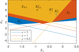
Figure 2: Stability regions $\mathcal{K}_{\rho}$, optimal feedbacks $K_{\rho}^{*}$ and stability boundaries $f_{1}=f_{2}=0$ for $\rho=0.5,\rho=1$ and $\rho=2$.

The set $\mathcal{C}$ obtained by Proposition 6, with $\mathcal{K}^{*}\subseteq\operatorname{int}(\mathcal{C})$ (see Remark 4), is given by $\mathcal{C}=[-0.94,-0.23]\times[4.49,5.97]$. Moreover, the condition $\mathcal{C}\subseteq\mathcal{K}_{\mathcal{P}}$ hold due to Proposition (5) and the obtained distances $d_{i}$ are depicted by solid black lines in Fig. 3.

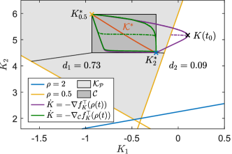
Figure 3: Visualization of the stability region $\mathcal{K}_{\mathcal{P}}$, the set $\mathcal{C}$ and trajectories of gradient flow and projected gradient flow for $\rho=0.5\to\rho=2$.

Quadratic stability of (42) is verified by Theorem 2 and the matrix $X=[0.9,-2.2;-2.2,7.7]$ satisfies the LMI condition (27) for all $\tilde{A}_{i},i=1,\dots,8$.

The trajectories of $\dot{K}=-\nabla f_{K}^{\top}(\rho)$ and $\dot{K}=-\nabla_{\mathcal{C}}f_{K}^{\top}(\rho)$ are shown for $K(0)=K^{*}_{0.5}$ in Fig. 3, where the parameter switches from $\rho=2$ to $\rho=0.5$. For the solid lines, the switch occurs after convergence to $K^{*}_{2}$ and $K^{*}_{0.5}$ is reached. For the dashed lines, the switch occurs prematurely at $t_{0}$, where the non-projected gradient flow yields $K(t_{0})$ outside the stability region $\mathcal{K}_{0.5}$ (see Fig. 3), leading to ill-defined behavior. Strictly speaking, the integral of the LQR cost $f_{K}(\rho(t))$ diverges due to the unstable feedback $K(t_{0})$, and the derivative $\nabla f_{K}(t_{0})$ is not defined. However, using vectorization, a negative LQR cost is observed, which is impossible by definition, and the cost diverges to $-\infty$ at the boundary of $\mathcal{K}_{0.5}$, where the trajectory reaches a steady state. In contrast, the projected gradient flow remains well-defined and converges to $K^{*}_{0.5}$ after the switch at $t_{0}$.

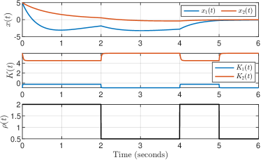
Figure 4: Trajectories of the states $x(t)$ and the feedback gains $K(t)$ for the fast-varying parameter trajectory $\rho(t)$.

Fig. 4 shows the trajectories of $x(t)$ and $K(t)$ for a fast-varying parameter trajectory $\rho(t)$ with step changes. A high learning rate ($\alpha\!=\!100$) ensures that $K(t)$ quickly converges to the optimal feedback during constant parameter intervals (see Remark 5). The dynamic controller yields an LQR cost of 488.9 over the $6\text{\,}\mathrm{s}$ simulation, significantly lower than the 660.3 obtained with the static feedback controller $K_{1.25}^{*}$. This $26\text{\,}\mathrm{\char 37\relax}$ reduction demonstrates improved transient performance.

VI Conclusion

This paper proposes a novel dynamic state-feedback controller for polytopic LPV systems based on a projected policy gradient flow that continuously minimizes the LQR cost while providing stability guarantees. We established conditions for quadratic stability of the LPV system that ensures exponential stability for arbitrarily fast-varying parameter trajectories. Sufficient conditions were also provided to ensure bounded trajectories of the controller and its convergence to the optimal feedback gains. Additionally, we proved asymptotic stability of the frozen-time closed-loop systems. Simulation results showcased the effectiveness of the controller in maintaining stability and improving transient performance.

-A Routh-Hurwitz Stability Criterion

The criterion states that a monic polynomial $p(s)=s^{n}+c_{1}s^{n-1}+c_{2}s^{n-2}+\ldots+c_{n-1}s+c_{n}$ has roots with negative real parts if and only if all the entries in the first column of the Routh table are strictly positive [29, Sec. 6.2-6.5]. The Routh table, with entries denoted by $R_{i,j}$, is constructed as follows

$$\begin{split}\begin{matrix}s^{n}&1&c_{2}&c_{4}&c_{6}&\cdots\\ s^{n-1}&c_{1}&c_{3}&c_{5}&\cdots\\ s^{n-2}&R_{3,1}&R_{3,2}&R_{3,3}&\cdots\\ s^{n-3}&R_{4,1}&R_{4,2}&R_{4,3}&\\ \vdots&\vdots&\vdots&\vdots\\ s^{1}&R_{n,1}&R_{n,2}&\\ s^{0}&c_{n}&\end{matrix},\end{split}$$ (43)

where $R_{i,j}=\left(R_{i-1,1}R_{i-2,j+1}-R_{i-2,1}R_{i-1,j+1}\right)/R_{i-1,1}$ for $3\!\leq\!i\!\leq\!n$, $1\!\leq\!j$, and missing terms are treated as zero.

References

- [1] Christian Hoffmann and Herbert Werner “A Survey of Linear Parameter-Varying Control Applications Validated by Experiments or High-Fidelity Simulations” In IEEE Transactions on Control Systems Technology 23.2, 2015, pp. 416–433
- [2] “Control of Linear Parameter Varying Systems with Applications” Springer Science & Business Media, 2012
- [3] Corentin Briat “Linear Parameter-Varying and Time-Delay Systems: Analysis, Observation, Filtering & Control” 3, Advances in Delays and Dynamics Springer, 2015
- [4] D. J. Leith and W. E. Leithead “Survey of gain-scheduling analysis and design” In Int. J. Control 73.11 Taylor & Francis, 2000, pp. 1001–1025
- [5] Jeff S. Shamma “Analysis and Design of Gain Scheduled Control Systems”, 1988
- [6] J.S. Shamma and M. Athans “Gain scheduling: potential hazards and possible remedies” In IEEE Control Systems Magazine 12.3, 1992, pp. 101–107
- [7] Fen Wu “Control of Linear Parameter Varying Systems”, 1995
- [8] A. Ilchmann, D.H. Owens and D. Prätzel-Wolters “Sufficient conditions for stability of linear time-varying systems” In Systems & Control Letters 9.2, 1987, pp. 157–163
- [9] Andrew P. White, Guoming Zhu and Jongeun Choi “Linear Parameter-Varying Control for Engineering Applications”, SpringerBriefs in Electrical and Computer Engineering, 2013
- [10] Wilson J. Rugh and Jeff S. Shamma “Research on gain scheduling” In Automatica 36.10, 2000, pp. 1401–1425
- [11] Fen Wu, Xin Hua Yang, Andy Packard and Greg Becker “Induced -norm control for LPV systems with bounded parameter variation rates” In International Journal of Robust and Nonlinear Control 6.9-10, 1996, pp. 983–998
- [12] P. Apkarian and R.J. Adams “Advanced gain-scheduling techniques for uncertain systems” In IEEE Transactions on Control Systems Technology 6.1, 1998, pp. 21–32
- [13] E. Feron, P. Apkarian and P. Gahinet “Analysis and synthesis of robust control systems via parameter-dependent Lyapunov functions” In IEEE Trans. Autom. Control 41.7, 1996, pp. 1041–1046
- [14] Franco Blanchini and Stefano Miani “Stabilization of LPV Systems: State Feedback, State Estimation, and Duality” In SIAM Journal on Control and Optimization 42.1, 2003, pp. 76–97
- [15] S.M Shahruz and S Behtash “Design of controllers for linear parameter-varying systems by the gain scheduling technique” In J. Math. Anal. Appl. 168.1, 1992, pp. 195–217
- [16] Carsten W Scherer “Mixed / control for time-varying and linear parametrically-varying systems” In International Journal of Robust and Nonlinear Control 6.9-10 Wiley Online Library, 1996, pp. 929–952
- [17] G. Becker and A. Packard “Robust performance of linear parametrically varying systems using parametrically-dependent linear feedback” In Syst. Control Lett. 23.3, 1994, pp. 205–215
- [18] P. Apkarian and P. Gahinet “A convex characterization of gain-scheduled controllers” In IEEE Transactions on Automatic Control 40.5, 1995, pp. 853–864
- [19] Pierre Apkarian, Pascal Gahinet and Greg Becker “Self-scheduled control of linear parameter-varying systems: a design example” In Automatica 31.9, 1995, pp. 1251–1261
- [20] C. Courties, J. Bernussou and G. Garcia “LPV control by dynamic output feedback” In Proc. Am. Control Conf. 4, 1999, pp. 2267–2271
- [21] E. Feron, V. Balakrishnan, S. Boyd and L. El Ghaoui “Numerical Methods for Related Problems” In 1992 American Control Conference, 1992, pp. 2921–2922
- [22] Earl Coddington and Norman Levinson “Theory Of Ordinary Differential Equations” McGraw-Hill, 1987
- [23] Jingjing Bu, Afshin Mesbahi and Mehran Mesbahi “Policy Gradient-based Algorithms for Continuous-time Linear Quadratic Control”, 2020 arXiv: https://arxiv.org/abs/2006.09178
- [24] Jingjing Bu, Afshin Mesbahi and Mehran Mesbahi “On Topological and Metrical Properties of Stabilizing Feedback Gains: the MIMO Case”, 2019 arXiv: https://arxiv.org/abs/1904.02737
- [25] H. Th. Jongen and Oliver Stein “Constrained Global Optimization: Adaptive Gradient Flows” In Frontiers in Global Optimization 74, 2003, pp. 223–236 Springer
- [26] Peter Lancaster and Leiba Rodman “Algebraic Riccati Equations” New York, USA: Oxford University Press Inc., 1995
- [27] James Munkres “Topology” Harlow, UK: Pearson Education Limited, 2014
- [28] Joao P Hespanha “Linear Systems Theory” Princeton, USA: Princeton University Press, 2018
- [29] Norman S Nise “Control Systems Engineering” John Wiley & Sons, 2019