Direct Algorithms for Reconstructing Small Conductivity Inclusions in Subdiffusion††thanks: The work of B. Jin is supported by Hong Kong RGC General Research Fund (Project 14306423), and a start-up fund from The Chinese University of Hong Kong.
Abstract
The subdiffusion model that involves a Caputo fractional derivative in time is widely used to describe anomalously slow diffusion processes. In this work we aim at recovering the locations of small conductivity inclusions in the model from boundary measurement, and develop novel direct algorithms based on the asymptotic expansion of the boundary measurement with respect to the size of the inclusions and approximate fundamental solutions. These algorithms involve only algebraic manipulations and are computationally cheap. To the best of our knowledge, they are first direct algorithms for the inverse conductivity problem in the context of the subdiffusion model. Moreover, we provide relevant theoretical underpinnings for the algorithms. Also we present numerical results to illustrate their performance under various scenarios, e.g., the size of inclusions, noise level of the data, and the number of inclusions, showing that the algorithms are efficient and robust.
keywords:
inclusion recovery, asymptotic expansion, direct algorithm, subdiffusion35R30, 65M32
1 Introduction
In this work, we aim at recovering small conductivity inclusions within a homogeneous background in subdiffusion processes. Let () be an open bounded Lipschitz domain with a boundary . Supose that there are small inclusions , , where and is a bounded Lipschitz domain in containing the origin, and let . The inclusions are assumed to be well separated from each other and from the boundary , i.e., there exist positive constants and such that for all , there holds
| (1) |
The background is homogeneous with a conductivity and the inclusion has a conductivity , where and are positive constants with , . The conductivity profile over the domain is given by
| (2) |
Consider the following initial boundary value problem:
| (3) |
where is the unit outward normal vector to the boundary , and the Neumann boundary data and the initial data satisfy the compatibility condition . Here denotes the left-sided Caputo fractional derivative of in time of order , defined by [16, p. 42]
where denotes Euler’s Gamma function. The model (3) is commonly known as the subdiffusion model, and can accurately describe anomalously slow diffusion processes. It has found many successful applications, e.g., solute transport in heterogeneous media [12, 6] and protein transport within membranes [24, 33]. The well-posedness of problem (3) in Sobolev spaces can be analyzed along the line of [25] and [16, Section 6.1].
The concerned inverse problem is to recover the locations of the inclusions from boundary measurement. It is related to nondestructive testing, i.e., locating anomalies inside a known homogeneous medium. This is a version of the inverse conductivity problem for the model (3). The uniqueness of identifying a general in the 1D case from one boundary flux was proved in [10]. The multi-dimensional case was studied in [28] and [9] for a general using the Dirichlet to Neumann map and a piecewise constant from one boundary flux, respectively. Kian et al [20] proved the unique determination of multiple coefficients from one boundary flux, excited by one specialized Dirichlet datum. Numerically, the reconstruction is commonly carried out using a regularized least-squares formulation. The numerical analysis of the schemes was given in [18, 17] for space-time or terminal data. Cen et al [9] employed the level set method to recover a piecewise constant . The regularization procedure is very flexible and works well for general conductivities, but solving the resulting optimization problems can be computationally demanding.
In this work, we develop novel direct algorithms for imaging small conductivity inclusions from the boundary measurement defined in (4). First we derive an asymptotic expansion of with respect to the size of the inclusions, cf. Theorem 2.1, which forms the basis for constructing the direct algorithms. The derivation relies on the coercivity of the Caputo fractional derivative (i.e., Alikhanov’s inequality [2]). One natural choice of the test function in is the fundamental solution to the model (3), but its accurate evaluation is highly nontrivial. One crucial step towards developing efficient algorithms is to use approximate fundamental solutions (i.e., truncating the asymptotic expansion of the reduced Green function). We analyze the perturbation of due to the approximate fundamental solution, and give sufficient conditions on the truncation level and the source location to ensure a similar asymptotic expansion of the resulting boundary measurement . The leading-order terms of the new asymptotic expansions lend themselves to the development of two computationally tractable algorithms, one for locating one inclusion, and the other for locating multiple inclusions, in both 2D and 3D cases. Moreover, we provide theoretical underpinnings for the algorithms. The numerical results show that the algorithms can accurately predict the locations for both circular and elliptical inclusions. To the best of our knowledge, they represent first direct algorithms for an inverse conductivity problem associated with the model (3).
The asymptotic expansion of the solutions with respect to the size of small inclusions has been extensively studied for standard elliptic and parabolic problems; see the monographs [4, 5] for in-depth treatments. The resulting asymptotic expansion can serve as a powerful computational tool for recovering the locations and shapes of small inclusions in elliptic and parabolic problems. Ammari et al [3] developed direct algorithms to recover the locations of small conductivity inclusions in the heat equation in the 2D case from boundary measurement, and analyzed the properties of the algorithms. Bouraoui et al [7, 8] extended the approach in [3] to identify locations and shape properties of small polygonal conductivity defects in the heat equation from partial boundary measurement. In this work, we utilize asymptotic expansions to recover the locations of small inclusions, which extends the 2D algorithms of the work [3] to the subdiffusion case, and also provide new algorithms in the 3D case. This development requires several tools from fractional calculus (e.g., integration by parts formula and Alikhanov’s inequality) and delicate analysis of the approximate fundamental solution, and the analysis of the algorithms is highly involved. These also represent the main technical novelties of the study.
The rest of the paper is organized as follows. In Section 2, we present an asymptotic analysis of the boundary measurement. In Section 3, we develop two direct algorithms for recovering small inclusions and provide relevant theoretical underpinnings. In Section 4, we present numerical experiments to complement the theoretical analysis. Finally, we give concluding remarks in Section 5. Throughout, denotes the space of absolutely continuous functions on . For any , denotes the right-sided Caputo derivative defined by
The notation denotes a generic constant which may change at each occurrence but it is always independent of .
2 Asymptotic expansion of boundary measurement
Now we establish the asymptotic expansion of the boundary measurement with respect to the size of small inclusions. This result will inspire the construction of direct imaging algorithms in Section 3.
2.1 Asymptotic expansion
To reconstruct the inclusions, we define the boundary measurement
| (4) |
where denotes surface integral, is a test function to be suitably chosen, and is the background solution satisfying
| (5) |
Throughout, and are taken to be smooth functions with continuous derivatives on the cylindrical domain . The existence, uniqueness and regularity of the solutions and to problems (3) and (5) can be found in [29, Theorems 3.5, 3.8 and 3.11].
We also define for and , which is the unique solution to
| (6) |
where is the outward unit normal vector to , and the subscripts and indicate the limit value as approaches from outside and from inside , respectively. Let
| (7) |
Then on the interface , the following two identities hold:
For , let
The matrix is known as the Pólya-Szegö polarization tensor associated with the inclusion and the conductivity [31]. The properties of were studied in [4, Chapter 3]. If the inclusion is a disk, then with being the identity matrix, is given by
| (8) |
We have the following asymptotic expansion of as under a mild condition on . Below we use the shorthand notation for , and for .
Theorem 2.1.
Let the test function satisfy
| (9) |
Then, for each fixed , with , there holds as
| (10) |
2.2 Proof of Theorem 2.1
First we recall several preliminary results on fractional calculus. See the monographs [30, 21, 16] for further details. We often use the Riemann-Liouville fractional integral of order , defined by [16, p. 22]
Then the following version of the fundamental theorem of calculus holds [16, Theorem 2.13]:
| (11) |
The next result gives an a priori estimate. We define the norm by
Lemma 2.2.
For , , and , let solve
| (12) |
Then there exists depending on , , and the Lipschitz character of and such that the following estimate holds
Proof 2.3.
By integration by parts, divergence theorem and the governing equation (12) for , we obtain
By Green’s identity on the subdomain , we obtain
By Alikhanov’s inequality [2, Lemma 1]
we have for all ,
Then the Cauchy-Schwarz inequality, and the trace inequality (for ) [14] imply
and similar bounds on the terms , . Consequently,
| (13) |
for some . Clearly, we have for any ,
| (14) |
Then, the choice , the identity (14) with and (11) give
Using the estimate (2.3) and Young’s inequality, we arrive at
which completes the proof of the lemma by choosing sufficiently small.
The next result gives an integral representation of the boundary measurement .
Lemma 2.4.
Proof 2.5.
The next result gives a crucial asymptotic expansion.
Lemma 2.6.
Proof 2.7.
The proof is based on mathematical induction on the number of inclusions. Actually we shall prove a stronger assertion (23). In the induction step, Lemma 2.2 plays a crucial role. Specifically, for any fixed , , and , let , be the solution to problem (3) with the presence of the first inclusions , for , and let
with . Also let for , with . For each fixed , with , the function satisfies
where the functions , , and are given by
It follows directly from Lemma 2.2 that
| (18) | ||||
Next we bound the first four terms of the inequality (18) for each fixed . Let . Note that due to the assumption (1). Moreover, since is bounded and as for each and , there exist such that
i.e., Then, changing variables leads to
| (19) | ||||
Let . Then similarly, due to the assumption (1), we have
Consequently,
| (20) | ||||
Next, note that the following identity holds:
Since for with (due to the assumption (1)), is bounded and as . Thus we have
Consequently, we deduce
| (21) | ||||
Furthermore, for each , since as , we have for due to (1). Hence,
| (22) | ||||
Note that the desired assertion (17) is one special case (with and ) of the following relation:
| (23) |
Below, we prove the assertion (23) by mathematical induction on . It suffices to estimate the last term in the fundamental estimate (18). For , we have . Note that
Then we deduce
| (24) |
Thus, the assertion (23) is proved for the case by combining the estimates (18)–(24). Now fix and assume that the assertion (23) holds for the case (instead of ). Then we have
| (25) |
Also, we have the identity
Since as , we have for with due to the assumption (1). Consequently,
| (26) | ||||
By repeating the argument for (24), we obtain
Also, the argument for the estimate (26) leads to
In addition, the induction hypothesis for the case gives
Combining the preceding three bounds yields
| (27) |
Finally, the assertion (23) is proved for all by the induction hypothesis for with (18)–(22) and (25)–(27). This completes the proof of the lemma.
Now we can give the proof of Theorem 2.1.
3 Direct reconstruction algorithms
Now we develop two direct algorithms for recovering small conductivity inclusions, and discuss relevant theoretical underpinnings.
3.1 Asymptotic expansions of fundamental solutions
The construction of the proposed algorithms relies on the fundamental solution to the model (3). For any , let be the fundamental solution satisfying
where denotes the Dirac delta function at . Let , with . Then by changing variables , we have
Thus, satisfies (9), and admits the asymptotic expansion (10) in Theorem 2.1. However, the accurate evaluation of is very challenging; see [1] for the 1D case (using Wright function). Thus, one has to use approximate fundamental solutions in the algorithms so as to ensure their computational tractability, and this greatly complicates the analysis of the algorithms. Following [32], we define the reduced Green function by
| (28) |
and we employ the following result from [32, Theorems 3.1 and 3.6]. Also the explicit expressions for the coefficients and for and can be found in [32, Remarks 3.2, 3.7 and Tables 1–2].
Lemma 3.1.
For any , there exist constants , with and such that the reduced Green functions for admit the following asymptotic expansions as :
Moreover, the asymptotics of can be obtained by termwise differentiation of .
We denote by the truncated asymptotic expansion of with terms (i.e., dropping the remainder in Lemma 3.1), and define the approximate fundamental solution with terms by
| (29) |
Below we take the test function . Note that no longer satisfies (9) for any and , and thus Theorem 2.1 does not directly apply to . We give suitable conditions on and to guarantee that the perturbation of is comparable with the remainder in (10) in Theorem 2.1 and that admits a similar asymptotic expansion. We shall see that this approximation requires the source point to be far away from , but is allowed to be small. The next result gives the expression of .
Lemma 3.2.
For each fixed and , is given by
where the auxiliary function is defined by for ,
Below we employ the boundary measurements for two choices of the background solution : harmonic functions and approximate fundamental solutions, and develop direct reconstruction algorithms based on these measurement data. We also provide relevant theoretical underpinnings. To indicate the dependence on , we use the notation .
3.2 Reconstructing one inclusion using harmonic functions
First we consider one inclusion for which we choose the background solution to be a harmonic function (i.e., ), with harmonic and time-independent such that . This choice has its origin in the constant current method [27]. We only discuss one circular inclusion, but the algorithm also works for inclusions of other shapes, cf. Section 4. To recover one circular inclusion of radius centered at , we take as the test function, with the truncation level and the source point properly chosen, and use measurements corresponding to background solutions , , where the vectors are linearly independent.
First we specify the assumption on and in .
Assumption 3.1.
and satisfy
| (30) | ||||
| (31) |
where the constants , and are independent of .
Below let , and for ,
with
Note that by [32, Remarks 3.2, 3.7], and thus over , the function is positive and attains the maximum at for fixed . Then for some constant , we have
| (32) |
Now we give an estimate of the perturbation due to the truncation of the approximate fundamental solution.
Lemma 3.4.
Proof 3.5.
From (28) and (29), we have, for all ,
| (34) | ||||
To estimate the right-hand side, by Lemmas 3.1 and 3.2, we derive, as ,
| (35) |
Note that and for . Also the estimate (31) in Assumption 3.1 gives
for independent of . By combining these relations with (34) and (35), we obtain, for sufficiently small ,
Finally, the condition (30) and the condition in Assumption 3.1 imply that, for sufficiently small ,
which gives the desired estimate (33).
The following theorem gives an asymptotic expansion of under Assumption 3.1.
Theorem 3.6.
Let Assumption 3.1 hold for and with sufficiently small . Then for any harmonic function , with satisfies
| (36) |
with . Furthermore, with , there exist , , and independent of such that
| (37) |
Proof 3.7.
Let . First, under Assumption 3.1, by (32) and the known asymptotics of [13, Section 2], we have uniformly in , and thus the assertion of Theorem 2.1 holds for . Next, using Lemma 2.6 and the trace lemma, we obtain the following estimate on defined in (16):
Moreover, the asymptotic relation as gives
Combining these relations gives
Then under Assumption 3.1 with sufficiently small , Lemma 3.4 yields
Next, Lemmas 3.1 and 3.2 with and (31) imply
| (38) |
with for some and independent of and . Moreover, by (38) with and (36) with the polarization tensor of one circular inclusion, cf. (8), we have
The relation (31) in Assumption 3.1 implies . Also note that for small enough, we have . These relations and (32) yield the inequality (37).
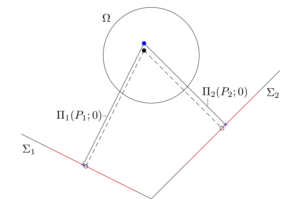
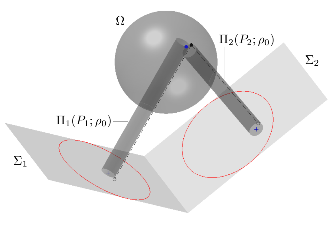
Now we describe a direct algorithm for locating one circular inclusion. We have measurements, corresponding to for . For , let be a line parallel to in 2D, and be a hyperplane orthogonal to in 3D. By the linear independence of , we have . The first step of the algorithm is to find the source point , , by solving the following equation for some :
| (39) |
The existence of a solution to (39) inside the orthogonal projection of onto for is given in Theorem 3.10(a) below. Let be the line if and the infinite cylinder of radius if , endowed with the axis of symmetry , . Let
Note that there always holds in 2D (i.e., is a line for ). The recovered location is given by
| (40) |
See Fig. 1 for schematic illustrations. We shall give an error estimate for this algorithm in Theorem 3.10(b). This algorithm in 2D is inspired by that in [4, Section 5.1]. We have extended it to the model (3) using and presented a new algorithm in 3D.
 |
 |
| (a) 2D | (b) 3D |
Next we discuss theoretical properties of the algorithm. We first give a result that motivates the construction of the algorithm. Let
| (41) |
be the leading-order term in (36), which approximates for small , cf. Theorem 3.6. The following result shows that the algorithm can exactly recover the location of the inclusion, if we use instead of when solving (39). Note that for , the remainder is absent, and the impact of on the reconstruction will be studied in Theorem 3.10.
Proposition 3.8.
Let . Then for , there exists a unique pair of solutions to (39) with replaced by . Furthermore, we have
The results also hold for any under the additional assumption .
Proof 3.9.
By [32, Remarks 3.2, 3.7 and Tables 1–2], the coefficients , and are all positive. Then there holds if and , or and . Then by the expression of in (8) (for a circular inclusion), the condition (and additionally in 3D) for is equivalent to (and also in 3D). This implies that is the orthogonal projection of onto , and hence .
Let be the orthogonal projection of onto for . In practice, the algorithm solves (39) using the data , , with for to obtain and , and to locate as (40). The following error bound on the recovered inclusion location holds.
Theorem 3.10.
Proof 3.11.
Let be as in Theorem 3.6. It follows from (37) that there exists such that for all , with , , there hold
| (42) | ||||
Next we discuss the 2D and 3D cases separately.
(i) 2D case. Let , with for , and be the line segment
| (43) |
Then is continuous on . By (42) and the intermediate value theorem, has at least one solution in . By the definition of , as , the line segment shrinks to , the projection of onto the line , and it is an interior point of , so part (a) holds in 2D. Let be any such pair of solutions. Since is in the region (43) for , the reconstruction defined by (40) satisfies
This and the condition implies the desired assertion in (b).
(ii) 3D case. For each , we consider the solid parallelogram
| (44) |
For each , the function , with , is continuous on . Note that for , every satisfies and . Then by (42) and Poincaré-Miranda theorem [26], has at least one solution in . As , the parallelogram shrinks to , which is again an interior point of , so part (a) also holds in 3D. Let be any such pair of solutions. Since for , the reconstruction satisfies
This and the condition imply the desired assertion in part (b).
Remark 3.12.
Theorem 3.10 requires linearly independent directions . The analysis shows that mutually orthogonal vectors lead to best conditioning for the reconstruction from the projection, and nearly parallel may impair the reconstruction accuracy.
3.3 Reconstructing multiple inclusions using approximate fundamental solutions
Now we consider the case of recovering multiple small circular inclusions. To this end, we choose the test function and the background solution for some with finitely many and properly chosen . The basic idea of the approach is related to the factorization method and MUSIC algorithm [23] in the sense that we shall construct an approximate indicator function to indicate the presence of small inclusions. We choose a truncation level and source points suitably, and obtain the data
| (45) |
with which we aim to reconstruct the locations of multiple inclusions. In the idealized case, i.e. choosing and for infinitely many , we can prove a sufficient criterion for locating inclusions. This important observation motivates the construction of an indicator function to indicate the inclusion locations in practice, using the finite amount of data (45). We focus the discussion on circular inclusions, but the algorithm is also applicable to inclusions of other shapes; see the numerical experiments in Section 4.
First we discuss the idealized case. Let be a nonempty open subset of , with . Let and be the Hilbert-Schmidt integral operators defined on , respectively, by
The operator serves as an idealized probing function to locate small inclusions from the measurement data. In view of the integral representation of in Lemma 2.4, the ranges of the operators and consist of analytic functions that analytically extend to and , respectively. We denote their extensions (to and , respectively) also by and . The next result gives a sufficient criterion for locating small conductivity inclusions. In the statement, we let
a ball centered at with a radius . Clearly is the set of inclusion centers. The proof of the theorem is technical and hence it is deferred to Appendix A.
Theorem 3.13.
For any , we have if, for every , the following identity holds
| (46) |
with
Further, for all , there exists an satisfying and some independent of such that
| (47) |
The second identity (47) in Theorem 3.13 shows that for all , the function has a singularity (only) at . The first identity (46) in Theorem 3.13 is obviously true for any in view of the inclusion and shows that if the singularity of is canceled out by with an optimal choice of and the degenerate size of the conductivity inclusions (i.e. ), then we have . This characterization of the set relies on the values of the functional inside , which are determined by the analytic extension from the open set . Instead of the singularity cancellation in the domain , we exploit the degeneracy of on the surface as a criterion for the numerical reconstruction of , which can be approximated using the discrete data , cf. (45). More precisely, we seek for points such that for each , the infimum of the functional over tends to zero as the inclusion size tends to zero. We restate the optimality of in terms of an orthogonal projection. Specifically, let be the orthogonal projection from onto the closure of the range of the operator . Theorem 3.13 suggests that an inclusion is located at if the mapping
blows up at , where denotes the Hilbert-Schmidt norm on , and is the identity operator. Thus, it provides an indicator function for locating the inclusion centers in the idealized case.
In practice, to use the finite data (45), we choose and suitably and construct an indicator function that approximates the mapping . The next result gives an asymptotic expansion of in (45), and its proof is similar to that of Theorem 3.6. Note that the leading-order term in (48) is a linear combination of the kernels of (see (8) for the expressions of for circular inclusions) but uses instead of .
Theorem 3.14.
Let and each point of satisfy Assumption 3.1 with sufficiently small . Then, for and with fixed , we have
| (48) |
with and moreover, for some independent of
with
To approximate the idealized indicator function , we need one additional assumption on the source points .
Assumption 3.2.
for all and , where is a family of pairwise disjoint open subsets of satisfying for all and for each fixed , and
Since a Hilbert-Schmidt integral operator with a square-integrable kernel is compact, is compact and admits Schmidt-representation [15, Theorem 1.1]
where is the sequence of positive singular values of (in descending order), and , are orthonormal singular vectors. Since forms an orthonormal basis of , we can define a sequence of projections onto by
The construction involves two steps: first approximate by
and then approximate by a fully discrete one. The next lemma is useful in analyzing the discrete approximation of .
Lemma 3.15.
Let be a sequence of compact linear operators on represented by
| (49) |
with positive singular values (ordered nonincreasingly) and orthonormal singular vectors , . If
then for each , we have
for some unitary transformations , where the constant depends only on the multiplicity of , and is the distance between and its nearest distinct singular value of .
Proof 3.16.
By [15, Corollary 1.6 in Chapter VI], we have
| (50) |
Let be the multiplicity of the -th singular value of , and for . From (50) and [11, Corollary 9], we deduce that for every , there exists an such that for all , ,
Thus, upon choosing some unitary transformations suitably, one can guarantee that for all , ,
with the constant .
To construct a discrete indicator function that approximates , for , we define for any
Also let be the matrix consisting of the leading left singular vectors of in (45), and . We construct a discrete indicator function by
| (51) |
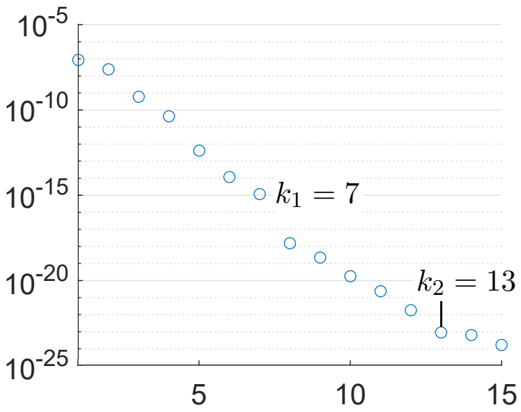
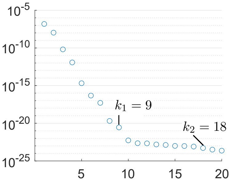
where denotes the Frobenius norm for matrices. In practice, the truncation level in the ratio (or ) is determined by the decay of the singular values of . The next result indicates that well approximates for and .
Theorem 3.17.
Let , , and . Suppose that Assumption 3.1 holds for and each point of with sufficiently small , and Assumption 3.2 holds for . Then, the following identities hold:
| (52) | ||||
| (53) |
where is the distance between and its nearest distinct singular value of , and the constants in in (52)–(53) are independent of .
Proof 3.18.
The integral kernels of the operators and are given, respectively, by
Let be the piecewise constant approximation of the kernel function defined almost everywhere on by
where is given in Assumption 3.2. Then, Assumption 3.2 implies
| (54) |
with
By Assumptions 3.1 and 3.2 and Lemmas 3.1 and 3.2, we obtain
| (55) |
where the constant in is independent of , , and . Combining the identity (54) with the estimate (55) gives the first desired relation (52).
Next, we define the following two operators and on : for any ,
For each , has finite rank and thus is compact. By [15, Theorem 1.1], admits the representation (49) for some positive sequence of descending order and orthonormal sequences . Then, the following identity holds:
By the triangle inequality, we get
| (56) | ||||
Now we estimate the two terms separately. First, the estimate (55) implies
| (57) | ||||
with the constant independent of . Thus is uniformly bounded (independent of ). Meanwhile, since the kernel function is smooth, Assumptions 3.1–3.2 and Lemmas 3.1–3.2 give
Thus, by Lemma 3.15, we have, for and ,
To bound , we define two kernel functions related to the operator :
Then, we have
In addition, by Theorem 3.14, we have
Combining the preceding three estimates gives
| (58) |
Finally, combining (57) and (58), we obtain (53) by letting in (56).
4 Numerical experiments and discussions
Now we present numerical results to illustrate the algorithms in Section 3. Throughout we take to be the unit disk , , and . We generate the data using a fully discrete scheme for problem (3) which employs the Galerkin finite element method with conforming linear elements in space and the L1 scheme in time [19, Chapters 2 and 4]. To accurately resolve the discontinuous conductivity, we employ finite element meshes graded around small inclusions, and divide the time interval into sub-intervals. The noisy data is generated by on , where the noise is randomly sampled in the finite element nodal values with a noise level , i.e., . Below we evaluate the algorithms in Sections 3.2 and 3.3 separately.
4.1 One inclusion
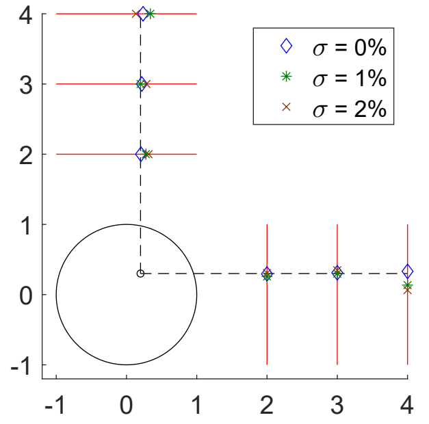
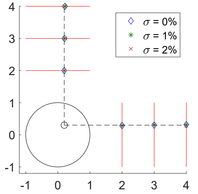
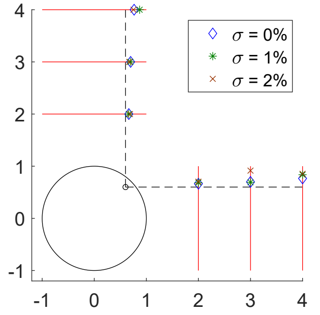
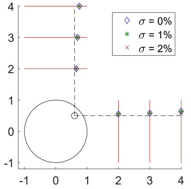
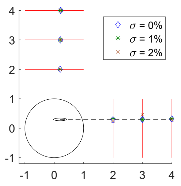
To recover one inclusion, we employ the data generated with two harmonic background solutions and , and the test function in for , where lies on the red line segment , cf. Fig. 2. We test the performance of the algorithm in Section 3.2.
Example 4.1.
Consider one circular inclusion , with four configurations . The conductivity is inside the inclusion.
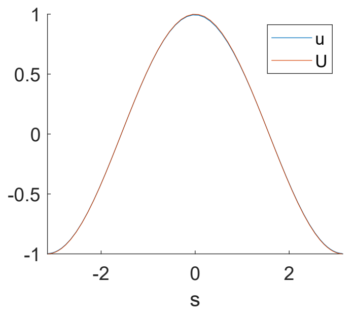
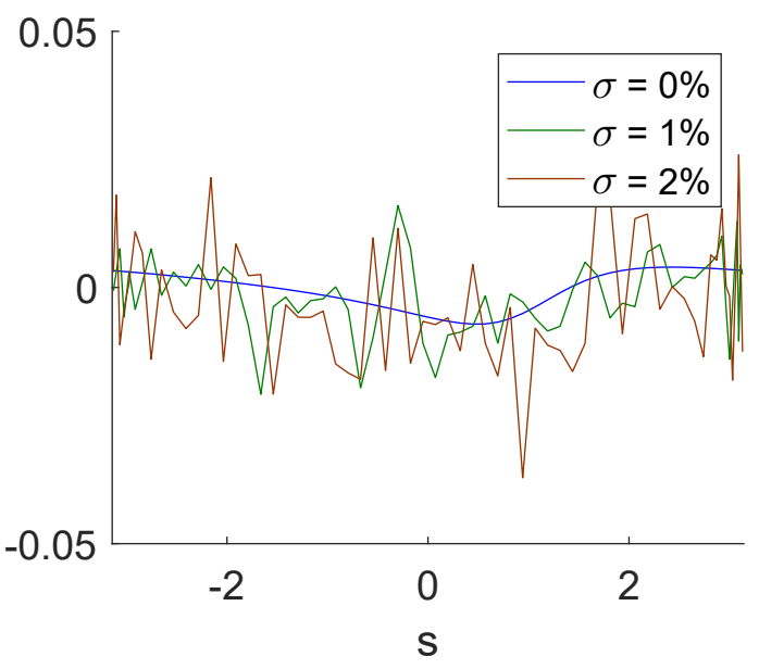
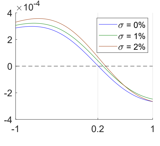
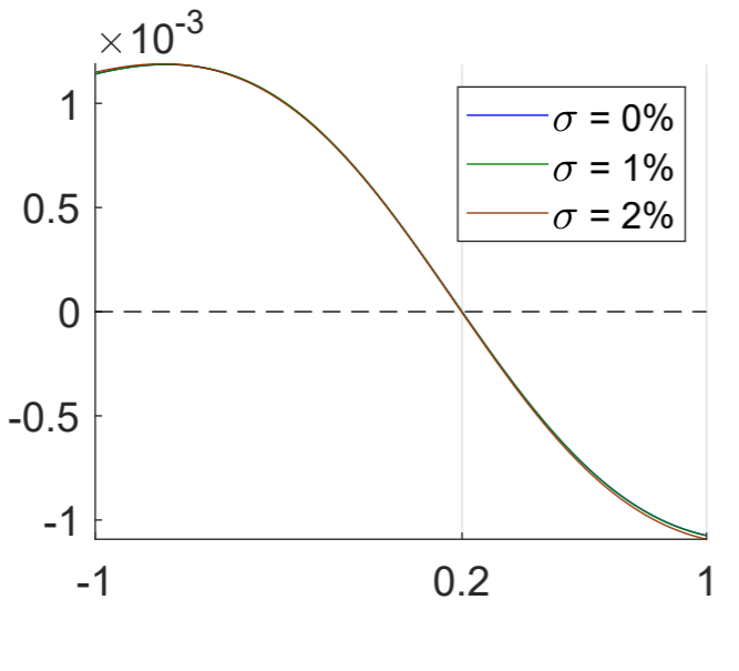
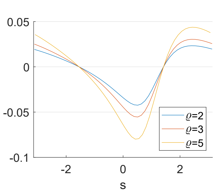
The reconstructions obtained by solving (39) are shown in Fig. 2. The inclusion locations are well resolved for both exact and noisy data. For the two cases and , we also show the impact of different noise levels on the data in Fig. 3. Note that the magnitude of increases with the size of the inclusion. Thus, in the presence of data noise of a fixed level , the noise appears relatively large for small inclusions, in view of the magnitude of the leading-order term in (36), and it can cause larger errors when solving for from (39), i.e., a bigger reconstruction error for a smaller inclusion. However, thanks to the beneficial smoothing effect of the weighted integral of in , the reconstruction obtained by solving (39) is fairly robust with respect to the additive noise in . Indeed, Fig. 3 shows that the values of are perturbed only very mildly even when the noise is relatively large compared with .
 |
 |
 |
 |
| (a) ((0.2,0.3),0.05) | (b) ((0.2,0.3),0.1) | (c)((0.6,0.6),0.05) | (d) ((0.6,0.5),0.1) |
 |
 |
 |
 |
 |
 |
 |
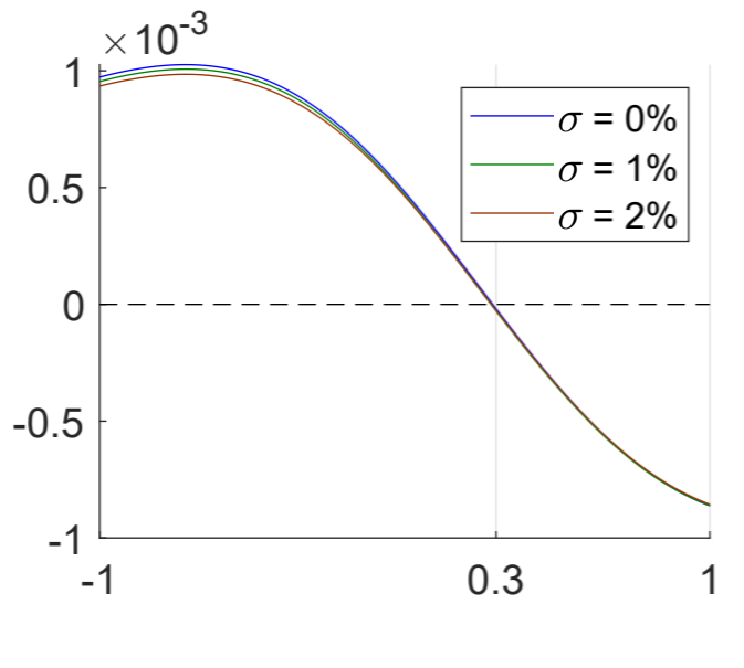 |
| (a) and | (b) | (c) versus | (d) versus |
Example 4.2.
Considers one elliptical inclusion , with an area and various aspect ratios . The conductivity inside the inclusion is .
 |
 |
 |
| (a) | (b) | (c) |
 |
 |
| (a) | (b) |
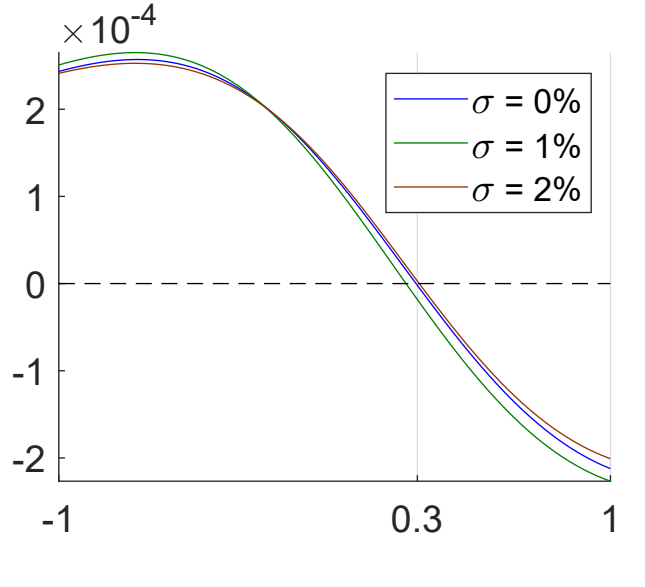
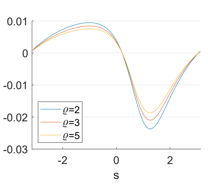
Fig. 4 shows the reconstruction results of one elliptical inclusion with various aspect ratios from noisy data. Interestingly, the reconstruction of the horizontal coordinate of the inclusion is more stable with respect to the noise than that of the vertical one. This can be explained by Fig. 5: the magnitude of is larger for than for for all aspect ratios . Then with a fixed level of noise, the noise is relatively larger for when than when , and thus the solution of is more stable with respect to the noise than that of . Nonetheless, the results in all cases are fairly good, and moreover, the algorithm in Section 3.2 is also applicable to non-circular inclusions.
4.2 Multiple inclusions
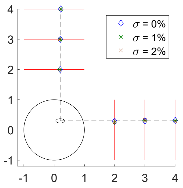
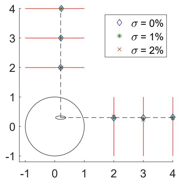
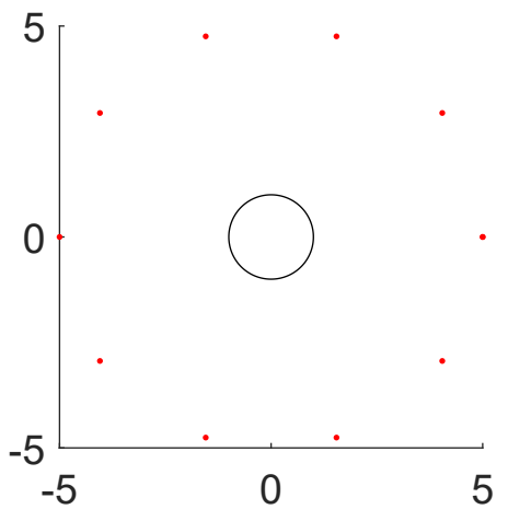
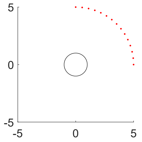
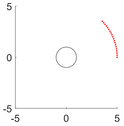
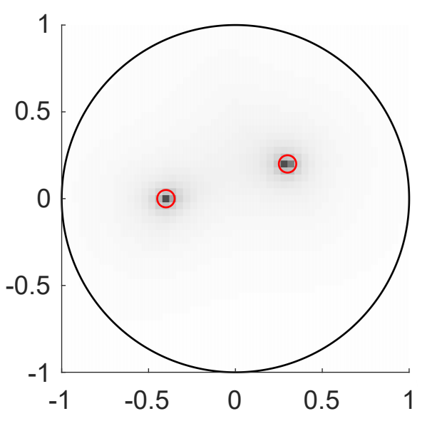
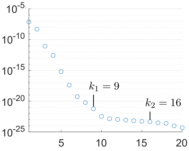
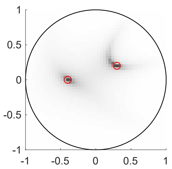
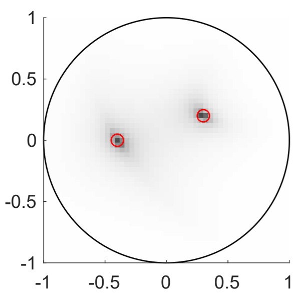
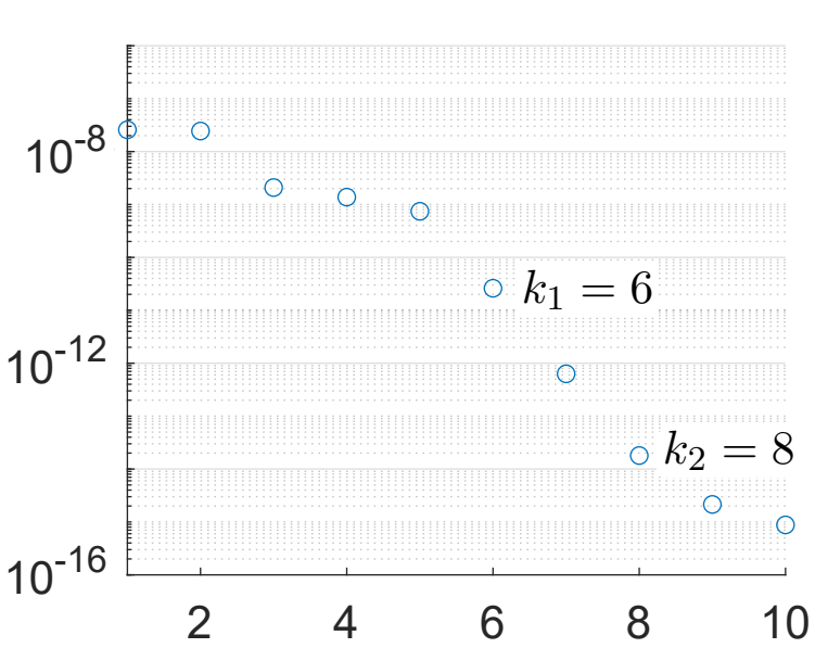
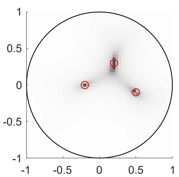
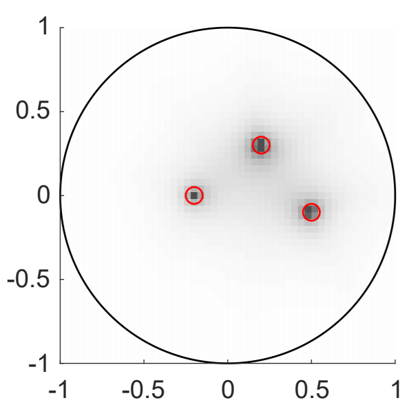
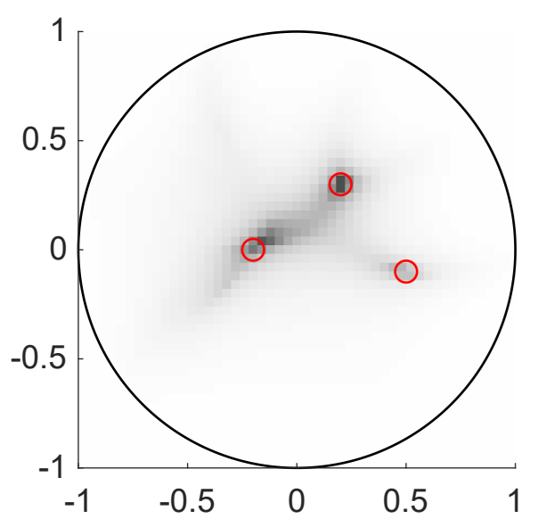
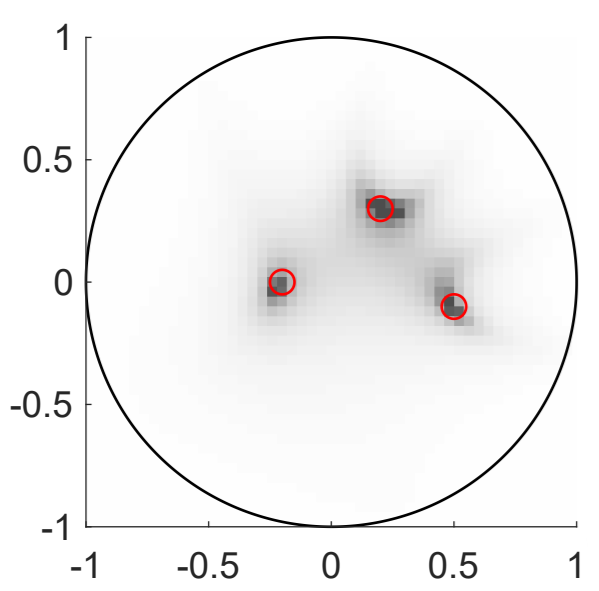
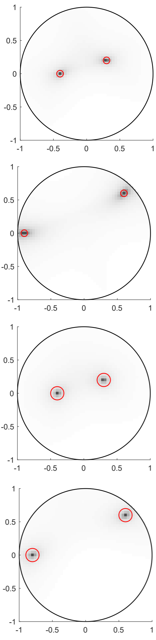
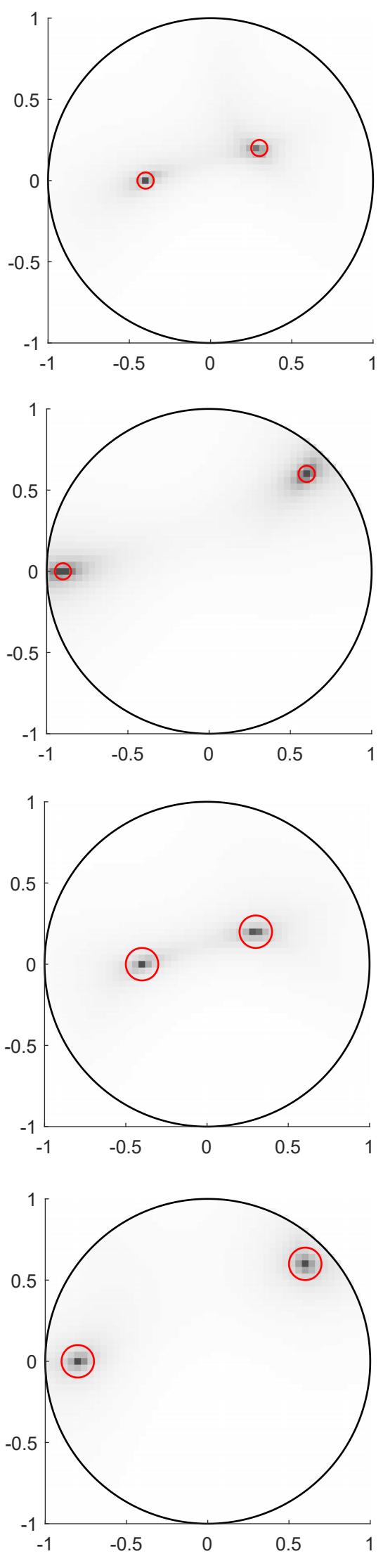
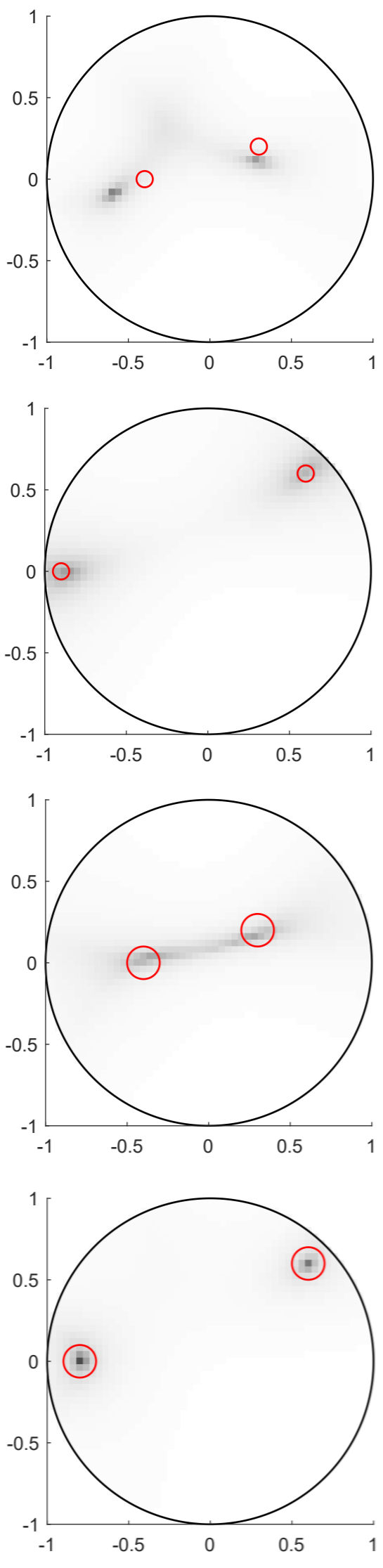
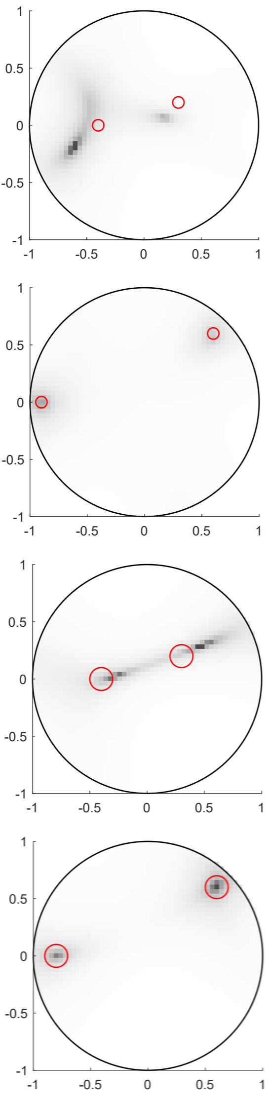
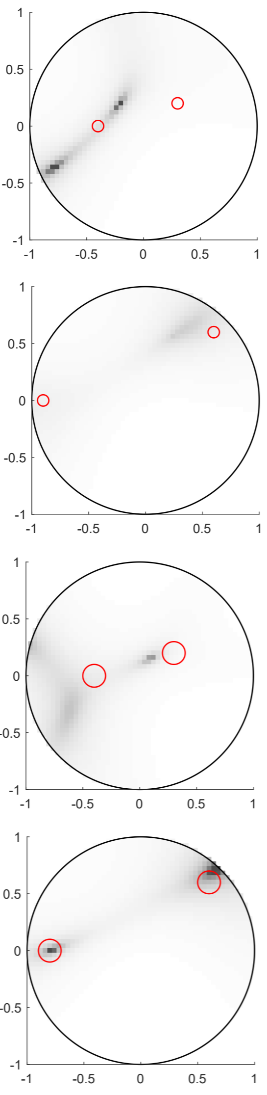
Now we consider the more challenging case of reconstructing multiple inclusions, using the algorithm in Section 3.3. The data are generated with the background solutions and the test function for . Below we fix at 10, and consider three configurations for the source points , cf. Fig. 6, including both full and limited aperture for measurement.
 |
 |
 |
| (i) | (ii) | (iii) |
Example 4.3.
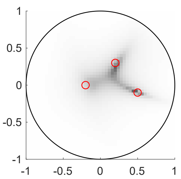
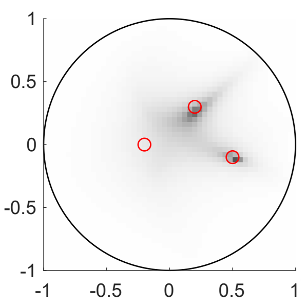
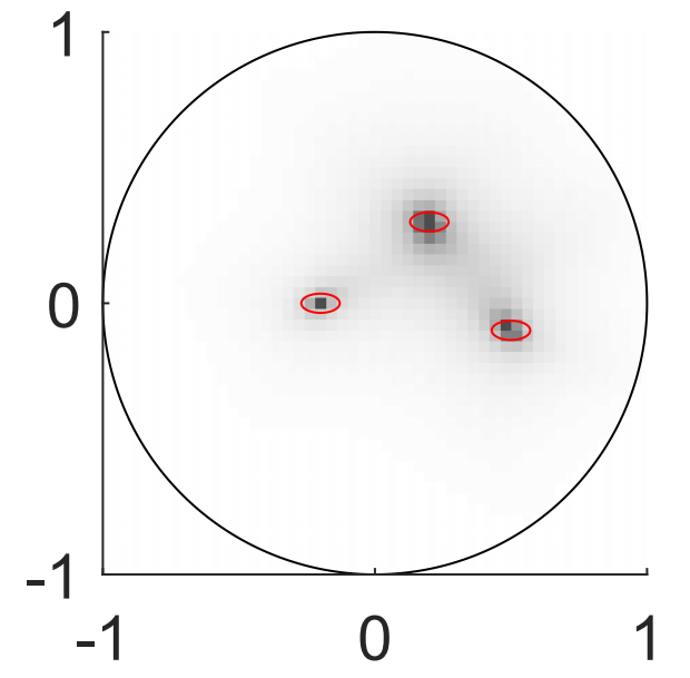
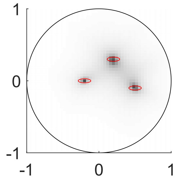
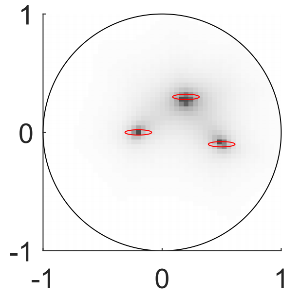
Consider circular inclusions , with and for , in two cases: (i) with and and (ii) with , and .
 |
 |
 |
 |
 |
 |
 |
 |
 |
| (a) singular values of | (b) | (c) |
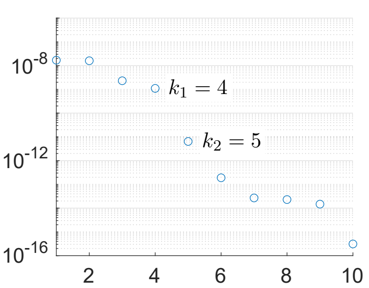
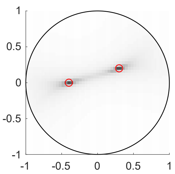
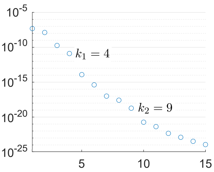
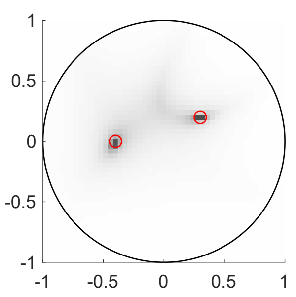
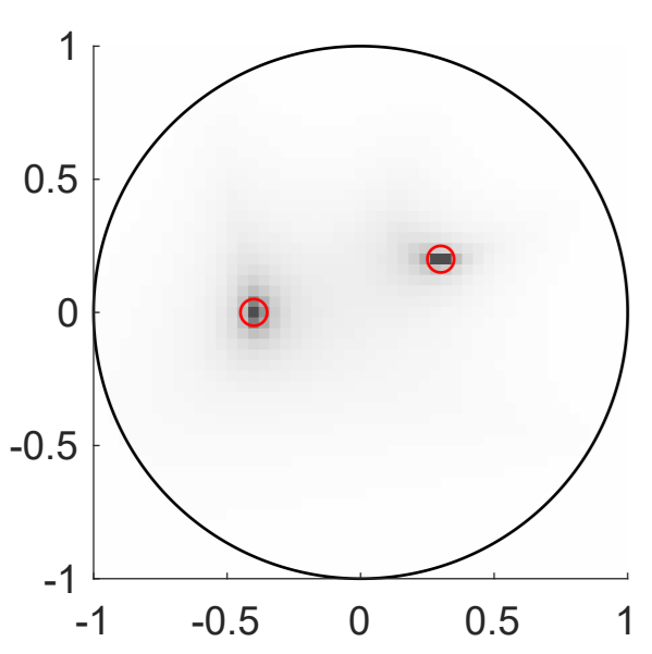
Figs. 7 and 8 show the reconstruction results for Example 4.3 (i) and (ii) with exact data, respectively. The singular values of (cf. (45)) decay rapidly, indicating its low-rank structure. With a suitable truncation level , the algorithm can accurately recover the locations, for all three configurations of observation apertures.
 |
 |
 |
 |
 |
 |
 |
 |
 |
| (a) singular values of | (b) | (c) |
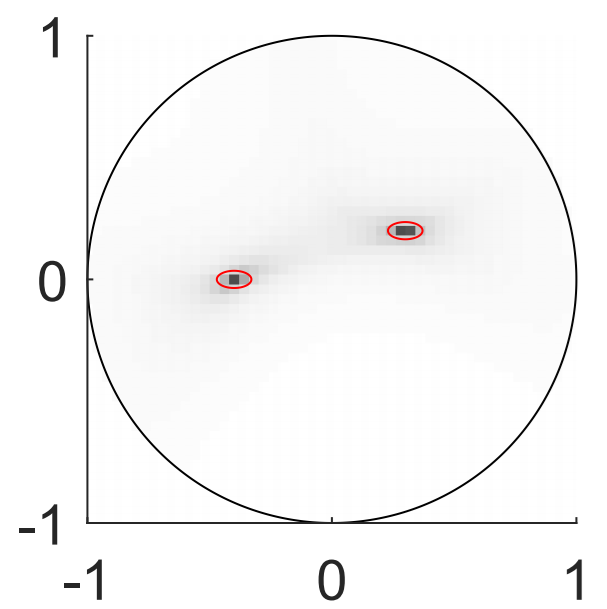
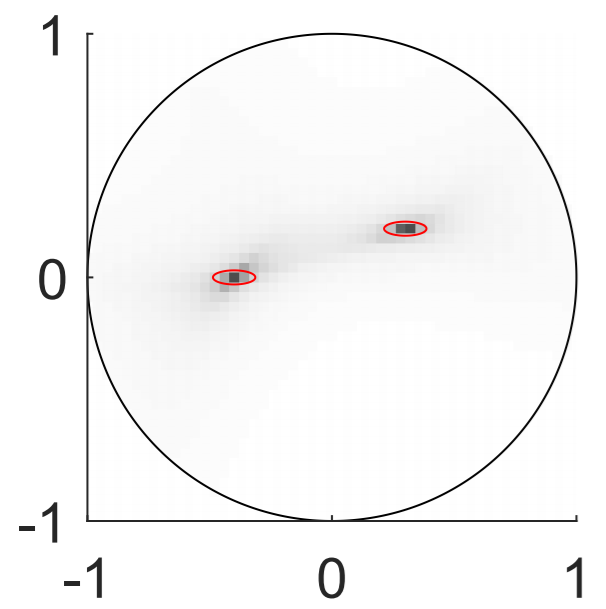
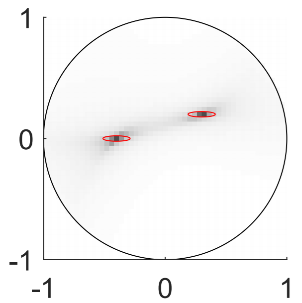
Example 4.4.
Consider two circular inclusions , where for , with . We consider different inclusion sizes and different locations .
In Fig. 9, we present the reconstruction results for Example 4.4, with the source points in Configuration (i) of Fig. 6. With a fixed level of noise, the recovery of the inclusion locations is more accurate either as the size of the inclusion increases or as the inclusions get closer to the boundary of the domain. This concurs with intuition that the inclusions with larger volume fractions or closer to the boundary generate stronger effective signals on the boundary and thus are easier to locate.
 |
 |
 |
 |
 |
Example 4.5.
Consider elliptical inclusions , with and for , where the aspect ratio , in two cases: (i) with and and (ii) with , and .
 |
 |
 |
 |
 |
 |
| (a) | (b) | (c) |
In Fig. 10, we show the reconstructions for Example 4.5 with exact data. The results indicate that the reconstructions remain fairly accurate for all the cases, even though the inclusions are not circular any more. Thus, the algorithm in Section 3.3 is also applicable to general inclusions other than circular ones.
5 Conclusion
In this work we have developed two direct algorithms for recovering the locations of small conductivity inclusions in the subdiffusion model from boundary measurement. The algorithms are based on the asymptotic expansion of the boundary measurement with respect to the size of small inclusions and essentially make use of approximate fundamental solutions. We have provided theoretical underpinnings for the algorithms for one and multiple circular inclusions. Several numerical experiments indicate that the algorithms can indeed accurately predict the locations of small circular and elliptical inclusions, including the case where data noise is present. Future works may include the analysis of the algorithms for more general conductivity inclusions as well as other types of measurements, e.g. partial boundary measurements or posteriori boundary measurements (i.e., over the time interval , with ).
Appendix A Proof of Theorem 3.13
We prove the two assertions by means of contradiction. Suppose that the identity (46) holds for some . Fix any , and let and be the characteristic function of the set . Since is a nonempty open set containing , we have . Choose any , and let be small enough so that . Then is analytic at , and hence
| (59) |
Meanwhile, by the definition of the operator , there holds
| (60) |
with
Note that the auxiliary function is smooth in since and satisfies for . Thus, we have
| (61) |
To bound the difference between (60) and (61), i.e., the integral , we split it into
| (62) |
where
with
Since for , we have . Since is smooth, there hold
| (63) |
Also from [22, Theorem 2.4 (i) and Theorem 2.5 (i-ii)], we have, for some and ,
| (64) |
By (63), (64) and changing variables from to , we derive
as . Similarly, we derive
as . Therefore, the right-hand side of (62) converges to as . This and the estimates (60)–(61) gives
| (65) |
Combining (65) with (59) gives
Then by the definition of , we have
where is independent of and . This contradicts the assumption (46). One can derive (47) in a similar way to (65).
References
- [1] L. Aceto and F. Durastante, Efficient computation of the Wright function and its applications to fractional diffusion-wave equations, ESAIM: Math. Model. Numer. Anal., 56 (2022), pp. 2181–2196.
- [2] A. Alikhanov, A priori estimates for solutions of boundary value problems for fractional-order equations, Differ. Equ., 46 (2010), pp. 660–666.
- [3] H. Ammari, E. Iakovleva, H. Kang, and K. Kim, Direct algorithms for thermal imaging of small inclusions, Multiscale Model. Simul., 4 (2005), pp. 1116–1136.
- [4] H. Ammari and H. Kang, Reconstruction of Small Inhomogeneities from Boundary Measurements, vol. 1846 of Lecture Notes in Mathematics, Springer-Verlag, Berlin, 2004.
- [5] , Polarization and Moment Tensors, Springer, New York, 2007.
- [6] B. Berkowitz, A. Cortis, M. Dentz, and H. Scher, Modeling non-fickian transport in geological formations as a continuous time random walk, Rev. Geophys., 44 (2006).
- [7] M. Bouraoui, L. El Asmi, and A. Khelifi, On an inverse boundary problem for the heat equation when small heat conductivity defects are present in a material, ZAMM Z. Angew. Math. Mech., 96 (2016), pp. 327–343.
- [8] M. Bouraoui, L. El Asmi, and A. Khelifi, Reconstruction of polygonal inclusions in a heat conductive body from dynamical boundary data, ESAIM Math. Model. Numer. Anal., 51 (2017), pp. 949–964.
- [9] S. Cen, B. Jin, Y. Liu, and Z. Zhou, Recovery of multiple parameters in subdiffusion from one lateral boundary measurement, Inverse Problems, 39 (2023), pp. 104001, 31.
- [10] J. Cheng, J. Nakagawa, M. Yamamoto, and T. Yamazaki, Uniqueness in an inverse problem for a one-dimensional fractional diffusion equation, Inverse Problems, 25 (2009), pp. 115002, 16.
- [11] D. K. Crane, M. S. Gockenbach, and M. J. Roberts, Approximating the singular value expansion of a compact operator, SIAM J. Numer. Anal., 58 (2020), pp. 1295–1318.
- [12] M. Dentz, A. Cortis, H. Scher, and B. Berkowitz, Time behavior of solute transport in heterogeneous media: transition from anomalous to normal transport, Adv. Water Res., 27 (2004), pp. 155–173.
- [13] S. D. Eidelman and A. N. Kochubei, Cauchy problem for fractional diffusion equations, J. Differential Equations, 199 (2004), pp. 211–255.
- [14] L. C. Evans and R. F. Gariepy, Measure Theory and Fine Properties of Functions, CRC Press, Boca Raton, FL, revised ed., 2015.
- [15] I. Gohberg, S. Goldberg, and M. A. Kaashoek, Classes of Linear Operators. Vol. I, Birkhäuser Verlag, Basel, 1990.
- [16] B. Jin, Fractional Differential Equations: an Approach via Fractional Derivatives, Springer, Cham, 2021.
- [17] B. Jin, X. Lu, Q. Quan, and Z. Zhou, Numerical recovery of the diffusion coefficient in diffusion equations from terminal measurement. Preprint, arXiv:2405.10708, 2024.
- [18] B. Jin and Z. Zhou, Numerical estimation of a diffusion coefficient in subdiffusion, SIAM J. Control Optim., 59 (2021), pp. 1466–1496.
- [19] , Numerical Treatment and Analysis of Time-Fractional Evolution Equations, Springer Nature, Cham, 2023.
- [20] Y. Kian, Z. Li, Y. Liu, and M. Yamamoto, The uniqueness of inverse problems for a fractional equation with a single measurement, Math. Ann., 380 (2021), pp. 1465–1495.
- [21] A. A. Kilbas, H. M. Srivastava, and J. J. Trujillo, Theory and Applications of Fractional Differential Equations, Elsevier Science B.V., Amsterdam, 2006.
- [22] K.-H. Kim and S. Lim, Asymptotic behaviors of fundamental solution and its derivatives to fractional diffusion-wave equations, J. Korean Math. Soc., 53 (2016), pp. 929–967.
- [23] A. Kirsch and N. Grinberg, The Factorization Method for Inverse Problems, Oxford University Press, Oxford, 2008.
- [24] S. C. Kou and X. S. Xie, Generalized Langevin equation with fractional Gaussian noise: subdiffusion within a single protein molecule, Phys. Rev. Lett., 93 (2004), p. 180603.
- [25] A. Kubica, K. Ryszewska, and M. Yamamoto, Time-Fractional Differential Equations—A Theoretical Tntroduction, Springer, Singapore, 2020.
- [26] W. Kulpa, The Poincaré-Miranda theorem, Amer. Math. Monthly, 104 (1997), pp. 545–550.
- [27] O. Kwon, J. K. Seo, and J.-R. Yoon, A real-time algorithm for the location search of discontinuous conductivities with one measurement, Comm. Pure Appl. Math., 55 (2002), pp. 1–29.
- [28] G. Li, D. Zhang, X. Jia, and M. Yamamoto, Simultaneous inversion for the space-dependent diffusion coefficient and the fractional order in the time-fractional diffusion equation, Inverse Problems, 29 (2013), pp. 065014, 36.
- [29] J. Mu, B. Ahmad, and S. Huang, Existence and regularity of solutions to time-fractional diffusion equations, Comput. Math. Appl., 73 (2017), pp. 985–996.
- [30] I. Podlubny, Fractional Differential Equations, Academic Press, Inc., San Diego, CA, 1999.
- [31] G. Pólya and G. Szegö, Isoperimetric Inequalities in Mathematical Physics, Princeton University Press, Princeton, 1951.
- [32] L. Qiu and J. Sim, A direct sampling method for time-fractional diffusion equation, Inverse Problems, 40 (2024), pp. 065006, 33.
- [33] K. Ritchie, X.-Y. Shan, J. Kondo, K. Iwasawa, T. Fujiwara, and A. Kusumi, Detection of non-brownian diffusion in the cell membrane in single molecule tracking, Biophys. J., 88 (2005), pp. 2266–2277.