A Preprocessing Framework for Efficient Approximate Bi-Objective Shortest-Path Computation in the Presence of Correlated Objectives

Abstract

The bi-objective shortest-path (BOSP) problem seeks to find paths between start and target vertices of a graph while optimizing two conflicting objective functions. We consider the BOSP problem in the presence of correlated objectives. Such correlations often occur in real-world settings such as road networks, where optimizing two positively correlated objectives, such as travel time and fuel consumption, is common. BOSP is generally computationally challenging as the size of the search space is exponential in the number of objective functions and the graph size. Bounded sub-optimal BOSP solvers such as A*pex alleviate this complexity by approximating the Pareto-optimal solution set rather than computing it exactly (given some user-provided approximation factor). As the correlation between objective functions increases, smaller approximation factors are sufficient for collapsing the entire Pareto-optimal set into a single solution. We leverage this insight to propose an efficient algorithm that reduces the search effort in the presence of correlated objectives. Our approach for computing approximations of the entire Pareto-optimal set is inspired by graph-clustering algorithms. It uses a preprocessing phase to identify correlated clusters within a graph and to generate a new graph representation. This allows a natural generalization of A*pex to run up to five times faster on DIMACS dataset instances, a standard benchmark in the field. To the best of our knowledge, this is the first algorithm proposed that efficiently and effectively exploits correlations in the context of bi-objective search while providing theoretical guarantees on solution quality.

1 Introduction and Related Work

In the bi-objective shortest-path (BOSP) problem (Ulungu and Teghem 1994; Skriver et al. 2000; Tarapata 2007), we are given a directed graph where each edge is associated with two cost components. A path $\pi$ dominates a path $\pi^{\prime}$ iff each cost component of $\pi$ is no larger than the corresponding component of $\pi^{\prime}$, and at least one component is strictly smaller. The goal is to compute the Pareto-optimal set of paths from a start vertex $v_{\text{s}}$ to a target vertex $v_{\text{t}}$, i.e., all undominated paths connecting $v_{\text{s}}$ to $v_{\text{t}}$.

BOSP models various real-world scenarios, such as minimizing both distance and tolls in road networks or finding short paths that ensure sufficient coverage in robotic inspection tasks (Fu et al. 2023).

A long line of research has extended the classical A* search algorithm to the multi-objective setting. MOA* (Stewart and White III 1991) and its successors (Mandow and De La Cruz 2008; Pulido, Mandow, and Pérez-de-la Cruz 2015) propose various techniques for improving performance, which were recently generalized into a unified framework (Ren et al. 2025).

BOSP is more challenging than single-objective search as it involves simultaneously optimizing two, often conflicting, objectives. The size of the Pareto-optimal solution set can be exponential in the size of the search space, making it computationally challenging to compute precisely (Ehrgott 2005; Breugem, Dollevoet, and van den Heuvel 2017).

While exact algorithms have been proposed for BOSP (Skyler et al. 2022; Hernández et al. 2023), we are often interested in approximating the Pareto-optimal solution set (see, e.g., (Perny and Spanjaard 2008; Tsaggouris and Zaroliagis 2009; Goldin and Salzman 2021)).

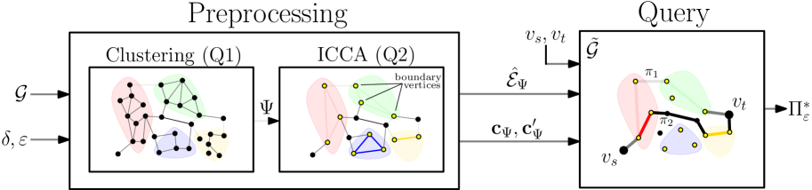
Figure 1: Illustration of the proposed algorithmic framework. An input graph $\mathcal{G}$ undergoes a preprocessing phase where regions with similar correlations are grouped into correlated clusters ($\Psi$) using an aggregation threshold ($\delta$). Subsequently, an Internal Cluster Cost Approximation (ICCA) process is performed for every correlated cluster to generate super-edges ($\hat{\mathcal{E}}_{\Psi}$) along with two cost functions ($\mathbf{c}_{\Psi},\mathbf{c}^{\prime}_{\Psi}$) for efficiently approximating (using a user-provided approximation factor $\boldsymbol{\varepsilon}$) the Pareto frontier of paths connecting the cluster’s boundary vertices. These are then used to construct a query graph $\tilde{\mathcal{G}}$ for efficiently computing $\Pi^{*}_{\boldsymbol{\varepsilon}}$, an approximation of the Pareto-optimal set for a bi-objective shortest-path query from $v_{\text{s}}$ to $v_{\text{t}}$.

We follow this line of work of approximating the Pareto-optimal solution set but focus on settings in which the objectives are positively correlated. Such correlations often exist in many real-world settings. For instance, in road networks, one may consider optimizing two positively correlated objectives such as travel time and fuel consumption. In the extreme case where there is perfect positive correlation between two objectives, the problem essentially collapses to a single-objective shortest-path problem and the Pareto-optimal set contains exactly one solution. Importantly, when the two objectives are strongly (though not perfectly) positively correlated, the Pareto-optimal set may contain many solutions but they are typically very similar in terms of their costs (Brumbaugh-Smith and Shier 1989; Mote, Murthy, and Olson 1991). Consequently, they can all be approximated by a single solution using a small value of approximation factor.

Surprisingly, despite the relevance to real-world applications and the potential to exploit correlation, this problem has largely been overlooked by the research community. Unfortunately, the correlation between the objectives can follow complex, non-uniform patterns that are challenging to exploit. Different regions of the graph can exhibit different levels of correlation, and their spatial distribution can significantly influence how large the approximation factor is required to be in order to approximate the entire Pareto frontier by a single solution.

Notable exceptions include empirical studies showing that, in the bi-objective setting, the cardinality of the Pareto-optimal set typically decreases as the positive correlation increases (Brumbaugh-Smith and Shier 1989; Mote, Murthy, and Olson 1991) and that, in the more general multi-objective setting, the size of the Pareto-optimal set increases significantly for negative (conflicting) correlations (Verel et al. 2013). Recently, Salzman et al. (2023) identified the potential of leveraging correlations to accelerate bi- and multi-objective search algorithms. To the best of our knowledge, our work is the first one to propose a practical, systematic approach to address this opportunity.

Our approach, summarized in Fig. 1, consists of a preprocessing phase and a query phase. In the preprocessing phase, regions, or clusters, of the bi-objective graph $\mathcal{G}$ with strong correlation between objectives are identified. The set of paths within each cluster that connect vertices that lie on the cluster’s boundary is efficiently approximated. In the query phase, a new graph is constructed that allows the search to avoid generating nodes within these clusters.

Key to our efficiency is a natural generalization of A*pex, a state-of-the-art approximate multi-objective shortest-path algorithm (Zhang et al. 2022). A*pex was chosen following its successful application in a variety of bi- and multi-objective settings (Zhang et al. 2024a, b, 2023a). We demonstrate the efficacy of our approach on the commonly-used DIMACS dataset, yielding runtime improvements of up to  $\times 5$ compared to running A*pex on the original graph.

2 Notation and Problem Formulation

We follow standard notation in BOSP (Salzman et al. 2023): Boldface indicates vectors, lower-case and upper-case symbols indicate elements and sets, respectively. $p_{i}$ is used to denote the $i$’th component of vector p.

Let $\textbf{p},\textbf{q}$ be two-dimensional vectors. We define their element-wise summation and multiplication as $\textbf{p}+\textbf{q}$ and $\textbf{p}\cdot\textbf{q}$, respectively. We say that p dominates q and denote this as $\textbf{p}\prec\textbf{q}$ iff $p_{1}\leq q_{1}$ and $p_{2}<q_{2}$ or if $p_{1}<q_{1}$ and $p_{2}\leq q_{2}$. When p does not dominate q, we write $\textbf{p}\nprec\textbf{q}$. For $\textbf{p}\neq\textbf{q}$, if $\textbf{p}\nprec\textbf{q}$ and $\textbf{q}\nprec\textbf{p}$, we say that p and q are mutually undominated. Given a set X of two-dimensional distinct vectors, we say that X is a mutually undominated set if all pairs of vectors in X are mutually undominated.

Let $\boldsymbol{\varepsilon}$ be another two-dimensional vector such that  $\varepsilon_{1},\varepsilon_{2}\geq~0$. We say that p $\boldsymbol{\varepsilon}$-dominates q and denote this as $\textbf{p}\preceq_{\boldsymbol{\varepsilon}}\textbf{q}$ iff $\forall i:\ p_{i}\leq(1+\varepsilon_{i})\cdot q_{i}$.

A bi-objective search graph is a tuple $\mathcal{G}=(\mathcal{V},\mathcal{E},\textbf{c})$, where $\mathcal{V}$ is the finite set of vertices, $\mathcal{E}\subseteq\mathcal{V}\times\mathcal{V}$ is the finite set of edges, and $\textbf{c}:\mathcal{E}\rightarrow\mathbb{R}^{2}_{\geq 0}$ is a cost function that associates a two-dimensional non-negative cost vector with each edge. A path $\pi$ from $v_{1}$ to $v_{n}$ is a sequence of vertices $v_{1},v_{2},\ldots,v_{n}$ such that $(v_{i},v_{i+1})\in\mathcal{E}$ for all $i\in~\{1,\ldots,n-1\}$. We define the cost of a path $\pi=v_{1},\ldots,v_{n}$ as $\textbf{c}(\pi)=\sum_{i=1}^{n-1}\textbf{c}(v_{i},v_{i+1})$. Finally, we say that $\pi$ dominates $\pi^{\prime}$ and denote this as $\pi\prec\pi^{\prime}$ iff $\textbf{c}(\pi)\prec\textbf{c}(\pi^{\prime})$.

Given a bi-objective search graph $\mathcal{G}=(\mathcal{V},\mathcal{E},\textbf{c})$ and two vertices $u,v\in\mathcal{V}$, we denote a minimal set of mutually undominated paths from $u$ to $v$ in $\mathcal{G}$ by $\Pi^{*}(u,v)$. Similarly, given an approximation factor $\boldsymbol{\varepsilon}$, we denote by $\Pi^{*}_{\boldsymbol{\varepsilon}}(u,v)$ a set of paths such that every path in $\Pi^{*}(u,v)$ is $\boldsymbol{\varepsilon}$-dominated by a path in $\Pi^{*}_{\boldsymbol{\varepsilon}}(u,v)$.

For the specific case of a query for start and target vertices $v_{\text{s}},v_{\text{t}}\in\mathcal{V}$ we set $\Pi^{*}:=\Pi^{*}(v_{\text{s}},v_{\text{t}})$ and $\Pi^{*}_{\boldsymbol{\varepsilon}}:=\Pi_{\boldsymbol{\varepsilon}}^{*}(v_{\text{s}},v_{\text{t}})$ and refer to them as a Pareto-optimal solution set and an $\boldsymbol{\varepsilon}$-approximate Pareto-optimal solution set, respectively. We call the costs of paths in $\Pi^{*}$ the Pareto frontier.

We call the problems of computing $\Pi^{*}$ and $\Pi^{*}_{\boldsymbol{\varepsilon}}$ the bi-objective shortest-path problem and bi-objective approximate shortest-path problem, respectively. In our work, we are interested in a slight variation of these problems where we wish to answer multiple bi-objective approximate shortest-path problems given a preprocessing stage. This is formalized in the following definition.

Problem 1.

Let $\mathcal{G}=(\mathcal{V},\mathcal{E},\textbf{c})$ be a bi-objective search graph and $\boldsymbol{\varepsilon}\in\mathbb{R}^{2}_{\geq 0}$ a user-provided approximation factor. Our problem calls for preprocessing the inputs $\mathcal{G}$ and $\boldsymbol{\varepsilon}$ such that, given a query in the form $v_{\text{s}},v_{\text{t}}\in\mathcal{V}$, we can efficiently compute $\Pi^{*}_{\boldsymbol{\varepsilon}}(v_{\text{s}},v_{\text{t}})$.

3 Algorithmic Background

This section provides the necessary algorithmic background for our framework. We begin in Sec. 3.1 by defining correlations between objectives in the context of graph search. Then, in Sec. 3.2, we overview A*pex.

3.1 Correlation in BOSP

Given two vectors $\mathbf{X}$ and $\mathbf{Y}$, the correlation coefficient $\rho_{\mathbf{X},\mathbf{Y}}$ quantifies the strength of their linear relationship (Pearson 1895), ranging from $-1$ (perfect negative correlation) to $1$ (perfect positive correlation). As $|\rho_{\mathbf{X},\mathbf{Y}}|$ approaches $1$, $\mathbf{X}$ and $\mathbf{Y}$ become more linearly dependent, meaning that $\mathbf{Y}$ can be closely approximated by a linear equation of the form $\mathbf{Y}=a\mathbf{X}+b$.

Definition 1 (correlation between objectives).

Let $E\subseteq\mathcal{E}$ be a set of edges such that each edge $e\in E$ is associated with cost $\textbf{c}(e)=\left(c_{1}(e),c_{2}(e)\right)$. Let $\boldsymbol{C_{1}}(E)$ ($\boldsymbol{C_{2}}(E)$ resp.) be a vector of size $|E|$ comprised of all $c_{1}(e)$ ($c_{2}(e)$ resp.) values of every edge $e\in E$. We define the correlation between objectives of the set $E$ as the correlation between vectors $\boldsymbol{C_{1}}(E)$ and $\boldsymbol{C_{2}}(E)$ and denote it as $\rho_{E}:=\rho_{\boldsymbol{C_{1}}(E),\boldsymbol{C_{2}}(E)}$.

Correlation between objectives is a common phenomenon. For instance, in the 9th DIMACS Implementation Challenge: Shortest Path dataset, a widely used benchmark in the BOSP research community, a strong correlation between objectives can be observed. Each instance in this dataset represents a road network graph from various areas in the USA and includes two objectives: driving time and travel distance. The correlation between objectives for an entire graph is roughly $\rho_{\mathcal{E}}~\approx~0.99$ for most DIMACS instances.

For brevity, when we mention a strong correlation, we specifically mean a strong positive correlation.

3.2 Approximating $\Pi^{*}$ using A*pex

In this section, we review A*pex (Zhang et al. 2022), a state-of-the-art multi-objective best-first search algorithm for approximating the Pareto-optimal solution set.

The efficiency of A*pex stems from how it represents subsets of the Pareto frontier using one representative path together with a lower bound on the rest of the paths in the subset. Specifically, an apex-path pair $\mathcal{AP}=\langle\mathbb{A},\pi\rangle$ consists of a cost vector $\mathbb{A}$, called the apex, and a path $\pi$, called the representative path. Conceptually, an apex-path pair represents a set of paths, that share the same start and final vertices, with its apex serving as the element-wise minimum of their cost vectors. We define the $\mathbb{g}$-value of $\mathcal{AP}$ as $\mathbb{g}(\mathcal{AP})=\mathbb{A}$ and $v(\mathcal{AP})$ to be the last vertex of $\pi$. The $\mathbb{f}$-value of $\mathcal{AP}$ is $\mathbb{f}(\mathcal{AP})=\mathbb{g}(\mathcal{AP})+\mathbb{h}(v(\mathcal{AP}))$. An apex-path pair $\mathcal{AP}$ is said to be $\boldsymbol{\varepsilon}$-bounded iff $\boldsymbol{c}(\pi)+~\mathbb{h}(v(\mathcal{AP}))\preceq_{\varepsilon}\mathbb{f}(\mathcal{AP})$.

A*pex maintains a priority queue Open, using $\boldsymbol{\varepsilon}$-bounded apex-path pairs as search nodes. At each iteration, A*pex extracts from Open the node $\mathcal{AP}=\langle\mathbb{A},\pi\rangle$ with the smallest $\mathbb{f}$-value. If the representative path $\pi$ has no chance to be part of the approximate solution set due to $\boldsymbol{\varepsilon}$-domination checks, the node is discarded. If it does and $v(\mathcal{AP})=v_{\text{t}}$, the node is added to the solution set. If none of the above holds, $\mathcal{AP}$ is expanded using each outgoing edge of $v(\mathcal{AP})$ to generate its successor apex-path pair $\mathcal{AP}^{\prime}=\langle\mathbb{A}^{\prime},\pi^{\prime}\rangle$. Formally, given an outgoing edge $e=~(v(\mathcal{AP}),v(\mathcal{AP}^{\prime}))$, $\mathcal{AP}^{\prime}$ is obtained by setting $\mathbb{A}^{\prime}$ to the element-wise sum of $\mathbb{A}$ and $\mathbb{c}(e)$, and setting $\mathbb{c}(\pi^{\prime})$ to the element-wise sum of $\mathbb{c}(\pi)$ and $\mathbb{c}(e)$ (see Fig. 2(a)). Since $\mathcal{AP}$ is $\boldsymbol{\varepsilon}$-bounded, $\mathcal{AP}^{\prime}$ is also $\boldsymbol{\varepsilon}$-bounded.

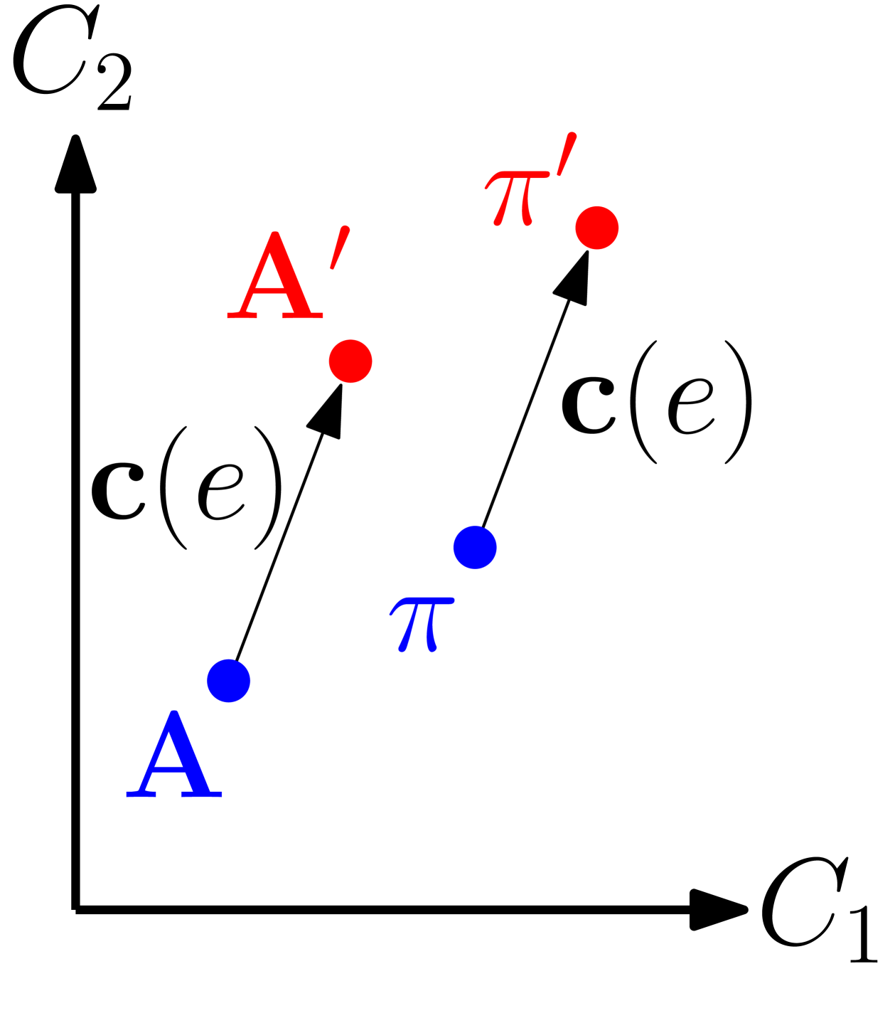
(a)

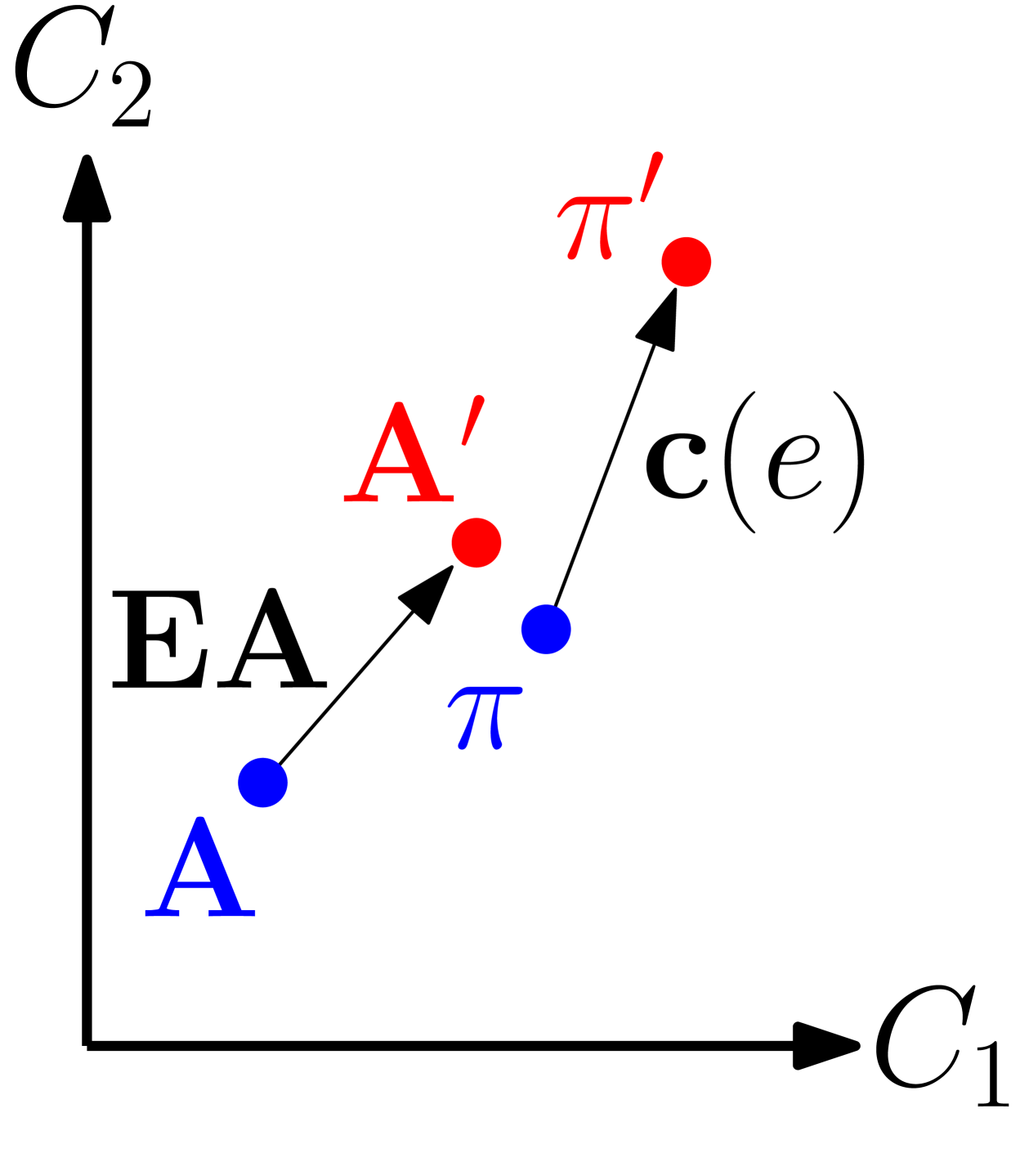
(b)

Figure 2: (a) A*pex expanding an apex-path pair $\mathcal{AP}=~\langle\mathbb{A},\pi\rangle$ by edge $e$ to obtain $\mathcal{AP}^{\prime}=\langle\mathbb{A^{\prime}},\pi^{\prime}\rangle$.
(b) GA*pex expanding an apex-path pair $\mathcal{AP}=\langle\mathbb{A},\pi\rangle$ by an apex-edge pair $\mathcal{AE}=\langle\mathbb{EA},{e}\rangle$ to obtain $\mathcal{AP}^{\prime}=\langle\mathbb{A^{\prime}},\pi^{\prime}\rangle$.

When A*pex adds an apex-path pair $\mathcal{AP}$ to Open, it first tries to merge $\mathcal{AP}$ with all other apex-path pairs in Open with the same $v(\mathcal{AP})$ to reduce the number of search nodes. When merging two apex-path pairs, the new apex is the element-wise minimum of the apexes of the two apex-path pairs, and the new representative path is either one of the original representative paths (see Fig. 3). If the resulting apex-path pair is $\boldsymbol{\varepsilon}$-bounded, the merged apex-path pair is used instead of the two original apex-path pairs.

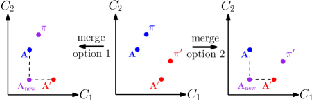
Figure 3: A*pex merge operation. The new apex-path pair’s representative path can be either $\pi$ or $\pi^{\prime}$.

When Open becomes empty, A*pex terminates and returns the representative paths of all apex-path pairs in the solution set as an $\boldsymbol{\varepsilon}$-approximate Pareto-optimal solution set.

4 Generalized A*pex (GA*pex)

As we will see, it will be useful to apply the notion of a representative path and an associated apex to arbitrary paths and not only to paths starting at $v_{\text{s}}$, for introducing super-edges. Thus, we introduce a natural generalization of edges which we call apex-edge pairs and show how apex-edge pairs can be seamlessly integrated into A*pex by generalizing the way A*pex expands apex-path pairs.

4.1 Apex-Edge Pair Description

Given vertices $u,v$, an apex-edge pair $\mathcal{AE}=\langle\mathbb{EA},{e}\rangle$ consists of a representative edge ${e}$ corresponding to a path connecting $u$ and $v$ and an edge apex $\mathbb{EA}$, which serves as a lower bound to a subset of the Pareto-optimal frontier of $\Pi^{*}(u,v)$. Similar to apex-path pairs, we say that an apex-edge pair $\mathcal{AE}$ is $\boldsymbol{\varepsilon}$-bounded iff $\mathbb{c}({e})\preceq_{\boldsymbol{\varepsilon}}\mathbb{EA}$.

We now generalize the expand operation of A*pex to account for apex-edge pairs. Let $\mathcal{AP}$ $=\langle\mathbb{A},\pi\rangle$ be an $\boldsymbol{\varepsilon}$-bounded apex-path pair, and let $\mathcal{AE}=\langle\mathbb{EA},{e}\rangle$ be an $\boldsymbol{\varepsilon}$-bounded apex-edge pair, where $e$ connects $v(\mathcal{AP})$ to some vertex $v^{\prime}$. Expanding $\mathcal{AP}$ by $\mathcal{AE}$ corresponds to a new apex-path pair $\mathcal{AP}^{\prime}=~\langle\mathbb{A^{\prime}},\pi^{\prime}\rangle$ where (i) $\pi^{\prime}:=\pi\cdot v$ with $\cdot$ denoting appending a vertex to a path, (ii) $\mathbb{c}(\pi^{\prime}):=\mathbb{c}(\pi)+\mathbb{c}({e})$, and (iii) $\mathbb{A}^{\prime}:=\mathbb{A}+\mathbb{EA}$ (see Fig. 2(b)).

Note. Given an edge $e$, we define the corresponding trivial apex-edge pair $\langle\mathbb{EA},e\rangle$ such that the edge apex $\mathbb{EA}$ equals $\mathbb{c}({e})$. Now, replacing every edge in a graph with the corresponding trivial apex-edge pair, the result of the expansion operation just described is identical to how A*pex expands apex-path pairs using edges. Similarly, running GA*pex (which we will describe shortly) when using only trivial apex-edge pairs is identical to how A*pex expands apex-path pairs using the corresponding edge.

4.2 Generalized A*pex

Formally, let $\mathcal{V}$ and $\mathcal{E}$ be a vertex set and edge set, respectively, and let $\mathbf{c},\mathbf{c^{\prime}}:\mathcal{E}\rightarrow\mathbb{R}^{2}_{\geq 0}$ be two bi-objective cost functions over the edge set $\mathcal{E}$ such that $\mathbf{c^{\prime}}(e)\preceq\mathbf{c}(e)$. We define $\hat{\mathcal{G}}:=(\mathcal{V},\mathcal{E},\mathbf{c},\mathbf{c^{\prime}})$ and refer to it as a generalized graph. For each edge $e$ in the generalized graph, we define the corresponding apex-edge pair $\mathcal{AE}=\langle\mathbb{EA},{e}\rangle$ such that $\mathbb{EA}$ and the cost of $e$ are $\mathbf{c^{\prime}}(e)$ and $\mathbf{c}(e)$, respectively.

In contrast to A*pex which runs on graphs, GA*pex runs on generalized graphs. However, the two algorithms only differ in how they expand apex-path pairs. Specifically, A*pex running on graph $\mathcal{G}=(\mathcal{V},\mathcal{E},\mathbf{c})$ is identical to GA*pex running on graph $\hat{\mathcal{G}}=(\mathcal{V},\mathcal{E},\mathbf{c},\mathbf{c^{\prime}})$ except that, when A*pex expands an apex-path pair using edge $e$, GA*pex expands the apex-path pair using $e$’s corresponding apex-edge pair.

Lemma 4.1.

Let $\mathcal{AP}=\langle\mathbb{A},\pi\rangle$ be an $\boldsymbol{\varepsilon}$-bounded apex-path pair, and let $\mathcal{AE}=\langle\mathbb{EA},{e}\rangle$ be an $\boldsymbol{\varepsilon}$-bounded apex-edge pair whose representative edge $e$ connects $v(\mathcal{AP})$ to some vertex $v^{\prime}$. If $\mathcal{AP}^{\prime}=~\langle\mathbb{A^{\prime}},\pi^{\prime}\rangle$ is the apex-path pair constructed by expanding $\mathcal{AP}$ by $\mathcal{AE}$, then $\mathcal{AP}^{\prime}$ is $\boldsymbol{\varepsilon}$-bounded.

Lemma 4.2.

Let $\mathcal{V}$ and $\mathcal{E}$ be a vertex set and edge set, respectively, and let $\mathbf{c},\mathbf{c^{\prime}}:\mathcal{E}\rightarrow\mathbb{R}^{2}_{\geq 0}$ be two bi-objective cost functions over the edge set $\mathcal{E}$ such that $\forall e\in\mathcal{E},\mathbf{c^{\prime}}(e)\preceq\mathbf{c}(e)$. Set $\boldsymbol{\varepsilon}:=\underset{e\in\mathcal{E}}{\max}\left(\mathbf{c}(e)/\mathbf{c^{\prime}}(e)-1\right)$. The Pareto-optimal solution set of paths between $v_{\text{s}}$ and $v_{\text{t}}$ in graph $\mathcal{G}=(\mathcal{V},\mathcal{E},\mathbf{c})$ is an $\boldsymbol{\varepsilon}$-approximation of the Pareto-optimal solution set of paths between $v_{\text{s}}$ and $v_{\text{t}}$ in graph $\mathcal{G}=(\mathcal{V},\mathcal{E},\mathbf{c^{\prime}})$.

Theorem 4.3.

Let $\hat{\mathcal{G}}=(\mathcal{V},\mathcal{E},\mathbf{c},\mathbf{c^{\prime}})$ be a generalized graph of graph $\mathcal{G}=(\mathcal{V},\mathcal{E},\mathbf{c})$. Let $v_{\text{s}},v_{\text{t}}\in~\mathcal{V}$ and recall that $\Pi^{*}$ denotes the Pareto-optimal set of paths connecting $v_{s}$ to $v_{t}$ in $\mathcal{G}$. Set $\boldsymbol{\varepsilon}:=\underset{e\in\mathcal{E}}{\max}\left(\mathbf{c}(e)/\mathbf{c^{\prime}}(e)-1\right)$ and let $\Pi^{*}_{\textsf{GA*pex}}$ be the output of GA*pex on $\hat{\mathcal{G}}$ when using an approximation factor $\boldsymbol{\varepsilon}$. Then, $\Pi^{*}_{\textsf{GA*pex}}\preceq_{\boldsymbol{\varepsilon}}\Pi^{*}$. Namely, running GA*pex on the generalized graph with approximation factor $\boldsymbol{\varepsilon}$ yields a Pareto-optimal solution set of paths between that is an $\boldsymbol{\varepsilon}$-approximation of the Pareto-optimal solution set of paths between in $\mathcal{G}$.

We omit the proofs of the lemmas and the theorem above.

5 Algorithmic Approach

In graph regions with a strong correlation between objectives, while there may be a large number of solutions in the Pareto-optimal solution set, they can typically all be $\boldsymbol{\varepsilon}$-dominated by a single solution using a small approximation factor. Following this insight, we propose an algorithmic framework (see Fig. 1) where, in a preprocessing phase (Sec. 5.1), we identify continuous regions with a strong correlation between objectives, which we call correlated clusters. To avoid having to run our BOSP search algorithm within each correlated cluster, we then compute a set of apex-edge pairs that allows the approximation of paths that traverse a correlated cluster. Given a query, these apex-edge pairs are used to construct a new graph, which we call the query graph, and to define a corresponding generalized query graph (Sec. 5.2). As we will see, running GA*pex on the generalized query graph allows us to compute $\Pi^{*}_{\boldsymbol{\varepsilon}}$ much faster than running A*pex on the original graph. The rest of this section formalizes our approach.

5.1 Correlation-Based Preprocessing

We start by introducing several key definitions.

Definition 2 (conforming edge).

Let $e\in\mathcal{E}$, $\delta>0$ be some threshold and $\ell$ be some two-dimensional line (i.e., $\ell:ax+by+1=0$ for some $a,b$ s.t. $a^{2}+b^{2}>0$). We say that an edge $e$ $\delta$-conforms with line $\ell$ iff $\texttt{dist}_{\perp}(\ell,\boldsymbol{c}(e))\leq\delta$. Here

$$\texttt{dist}_{\perp}(\ell,\boldsymbol{c}(e)):=\frac{|ac_{1}(e)+bc_{2}(e)+1|}{\sqrt{a^{2}+b^{2}}}.$$ (1)

Definition 3 (correlated cluster).

Given a graph $\mathcal{G}=(\mathcal{V},\mathcal{E})$, a $(\delta,\ell)$-correlated cluster of $\mathcal{G}$ is a subgraph $(V,E)$ of $\mathcal{G}$, s.t. (i) $V\subseteq\mathcal{V}$ and $E=(V\times V)\cap\mathcal{E}$ and (ii) $\forall e\in E$, we have that $e$ $\delta$-conforms with $\ell$.

As we will see, all the $(\delta,\ell)$-correlated clusters we will consider will use the same value of $\delta$. Thus, to simplify exposition and with a slight abuse of notation, we will refer to a $(\delta,\ell)$-correlated cluster $\psi$ simply as a cluster and use $\ell(\psi)$ to obtain the line that all edges of $\psi$ conform with.

Definition 4 (boundary vertices).

Let $\psi$ be a correlated cluster of $\mathcal{G}=(\mathcal{V},\mathcal{E})$. The set of boundary vertices of $\psi$ in $\mathcal{G}$, denoted as $B(\psi)$, is defined as

$$B(\psi):=\{u\in V_{\psi}\ |\ \exists v\in\mathcal{V}\setminus V_{\psi}~s.t.~(u,v)\in\mathcal{E}\ \text{or}\ (v,u)\in\mathcal{E}\}.$$

In other words, a vertex $u\in V_{\psi}$ is a boundary vertex iff it has at least one adjacent vertex $v\in\mathcal{V}\setminus V_{\psi}$.

In an $(\ell,\delta)$-correlated cluster of $\mathcal{G}$, small values of $\delta$ typically imply that the entire Pareto frontier of paths between the cluster’s boundary vertices can be approximated by a single solution, given a small $\boldsymbol{\varepsilon}$. This allows us to introduce a small number of apex-edge pairs that enable our approximate BOSP search algorithm to avoid expanding vertices within the correlated clusters.

Roughly speaking, we need to identify as many clusters as possible while maximizing their size. Large clusters can help reduce the search space by avoiding inner-cluster vertices. However, large clusters have boundary vertices that are far apart, what may lead to a large number of mutually-undominated paths. The preprocessing phase of our framework addresses two key questions:

1. How can we efficiently detect and delineate correlated clusters within the graph?

2. How can we efficiently compute an approximation of all mutually undominated paths connecting the boundary vertices of a cluster?

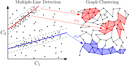
Figure 4: Detection and delineation of correlations between the two cost objectives (Q1). Left: a RANSAC-based approach is used to identify distinct linear modes in the 2D objectives space (Alg. 1). Right: the lines are then used for delineating correlated clusters within the graph.

Detecting and Clustering (Q1)

Algorithm 1 Multiple-line detection using RANSAC

Input:

1. Graph $\mathcal{G}=(\mathcal{V},\mathcal{E},\boldsymbol{c})$ where $\boldsymbol{c}$ is normalized

2. Allowed distance from the representative line $\delta$

3. Hyperparameters $n_{\text{hypotheses}}$, $n_{\text{min\_inliers}}$

Output: Set of identified line coefficients $\mathcal{L}$

1:$\mathcal{L}\leftarrow\emptyset$ $\triangleright$ Initialize set of detected lines

2:$E\leftarrow\mathcal{E}$ $\triangleright$ Initialize set of all edges

3:while ToContinue$()$ do

4:  $\mathcal{L}_{\text{candidates}}\leftarrow\emptyset$ $\triangleright$ Initialize candidate lines set

5:  for $m=1$ to $n_{\text{hypotheses}}$  do

6:   Sample two random edges $e_{i},e_{j}\in E$

7:   $\ell_{m}\leftarrow\texttt{LineFit}(e_{i},e_{j})$

8:   $\mathcal{I}_{m}\leftarrow\emptyset$ $\triangleright$ Initialize inliers set for $\ell_{m}$

9:   for each $e_{k}\in E$ do

10:     if $\texttt{dist}_{\perp}(\ell_{m},c(e_{k}))\leq\delta$ then $\triangleright$ Eq. (1)

11:      $\mathcal{I}_{m}\leftarrow\mathcal{I}_{m}\cup e_{k}$ $\triangleright$ Add $e_{k}$ as an inlier         

12:   if $|\mathcal{I}_{m}|>n_{\text{min\_inliers}}$ then

13:     $\mathcal{L}_{\text{candidates}}\leftarrow\mathcal{L}_{\text{candidates}}\cup\{(\ell_{m},|\mathcal{I}_{m}|)\}$      

14:  if $\mathcal{L}_{\text{candidates}}\neq\emptyset$ then

15:   Select $\ell^{*}$ from $\mathcal{L}_{\text{candidates}}$ with maximal inliers $\mathcal{I}^{*}$

16:   $\mathcal{L}\leftarrow\mathcal{L}\cup\ell^{*}$ $\triangleright$ Store best detected line

17:   $E\leftarrow E\setminus\mathcal{I}^{*}$ $\triangleright$ Remove inliers from sample set   

18:return $\mathcal{L}$

Given an input graph, our objective is to detect and delineate correlated clusters whose edges exhibit a strong correlation between objectives.

To motivate this step, consider a graph $\mathcal{G}=(\mathcal{V},\mathcal{E})$ containing two perfectly-correlated disjoint subsets $E_{1},E_{2}$ of $\mathcal{E}$. Since each set $E_{i}$ is perfectly correlated, all edge costs of $E_{i}$ lie on a line $\ell_{i}$ with parameters $a_{i},b_{i}$, which may differ. For example, time and distance may be perfectly correlated at any constant speed.

Merging $E_{1}$ and $E_{2}$ would not only break the perfect correlation in the group, but would also increase the minimal required $\boldsymbol{\varepsilon}$ for approximating the Pareto frontier of paths between boundary vertices using a single solution. The same argument holds even when the correlation is not perfect.

To this end, in order to detect distinct linear relationships in the 2-dimensional $(\boldsymbol{C_{1}},\boldsymbol{C_{2}})$ space, we utilize RANSAC (Random Sample Consensus) (Fischler and Bolles 1981), similar to Mahmood, Han, and Lee (2020). RANSAC is an iterative method for estimating model parameters from observed data while distinguishing inliers from outliers. In our case, it is adapted to distinguish between different linear relationships in the objective costs space.

Our RANSAC-based multi-line detection algorithm is summarized in Alg. 1. It takes as input a graph $\mathcal{G}$ with normalized edge costs, the allowed deviation threshold $\delta$, and two hyperparameters: $n_{\text{hypothesis}}$, the number of tested hypotheses before detecting a line and $n_{\text{min\_inliers}}$, the minimum number of inliers required to accept a detected line.

The algorithm iteratively samples two edges and fits a line through their 2D cost coordinates (Lines 6-7), ensuring a positive slope (i.e., a positive correlation). It then counts inliers - edges that $\delta$-conform with the fitted line (Lines 9-11). The fitted line with the most inliers is selected and added to $\mathcal{L}$, the set of detected lines (Lines 15-16). All corresponding inliers are then removed (Line 17), and the process repeats on the remaining data. This iterative procedure continues until termination conditions are met (Line 3), such as too few edges to sample from or reaching the iterations limit.

The left pane of Fig. 4 illustrates an example of two correlation lines identified using the proposed RANSAC method. Each line has a corresponding subset of cost samples that lie within a distance of up to $\delta$.

After computing $\mathcal{L}$ which captures the distinct linear relationships between objectives’ costs, our next step is to delineate the boundaries of the correlated clusters associated with each line. Inspired by Tarjan (1972), we propose a connected-components labeling algorithm for delineating the correlated clusters based on $\mathcal{L}$.

The algorithm maintains a set of unvisited graph vertices and terminates only when all vertices are visited. In each iteration, an unvisited vertex $u$ is randomly selected as the member of a new correlated cluster. Then, the algorithm examines all of $u$’s neighboring edges $E_{u}$. For each edge $e\in E_{u}$, we compute the set of lines $L_{u}\subset\mathcal{L}$ which $e$ conforms with. If there exists a line $\ell_{u}$ that all these edges conform to (i.e., $\bigcap_{e\in E_{u}}L_{u}\neq\emptyset$) then a new cluster $\psi_{u}$ is created and $u$ is added to the cluster’s vertex set. Now, a Depth-First Search (DFS) recursion is invoked for each neighboring vertex to expand the cluster. All neighbors are then removed from the set of unvisited vertices. This process is recursively repeated until not all of the current vertex’s neighboring edges conform to the cluster’s line $\ell_{u}$. Subsequently, a new vertex is randomly chosen from the unvisited vertices set, and the process repeats until all of the graph’s vertices are visited. The right pane of Fig. 4 illustrates an example of delineating three correlated clusters based on $\mathcal{L}$.

Internal Cluster Cost Approximation (ICCA) (Q2)

Let $\psi$ be a correlated cluster with vertices $\mathcal{V}_{\psi}$ and edges $\mathcal{E}_{\psi}$. For each boundary pair $b_{i},b_{j}\in B(\psi)$ we run A*pex with approximation factor $\boldsymbol{\varepsilon}$ on on the graph $(\mathcal{V}_{\psi},\mathcal{E}_{\psi})$. This yields a set of apex-path pairs $\mathcal{AP}^{1}_{i,j},\ldots,\mathcal{AP}^{n}_{i,j}$.

For each such apex-path pair $\mathcal{AP}^{k}_{i,j}=\langle\mathbb{A}^{k}_{i,j},\pi^{k}_{i,j}\rangle$, we introduce an edge which we call a super-edge $\hat{e}^{k}_{i,j}$ connecting $b_{i}$ to $b_{j}$ and associate it with two cost vectors $\mathbf{c}_{\psi},\mathbf{c^{\prime}}_{\psi}$ corresponding to the cost of the representative path and the apex-path pair’s apex, respectively.

Specifically, we set $\mathbf{c}_{\psi}(\hat{e}^{k}_{i,j}):=\mathbf{c}(\pi^{k}_{i,j})$ and $\mathbf{c^{\prime}}_{\psi}(\hat{e}^{k}_{i,j}):=\mathbf{c}(\mathcal{AP}^{k}_{i,j})$. We then set ${\hat{\mathcal{E}}_{\psi,i,j}}$ to be all the super-edges connecting $b_{i}$ and $b_{j}$ and ${\hat{\mathcal{E}}_{\psi}}:=\bigcup_{b_{i},b_{j}\in B(\psi),i\neq j}{\hat{\mathcal{E}}_{\psi,i,j}}$.

Example 1.

Consider the cluster $\psi$ depicted in Fig. 5, which contains three Pareto-optimal solution $\pi_{1},\pi_{2}$ and $\pi_{3}$ between $b_{i}$ and $b_{j}$ (Fig. 5(a)). Here, their costs are $(20,100),(80,30)$ and $(90,28)$, respectively. When running A*pex with an approximation factor of $\boldsymbol{\varepsilon}=[0.1,0.1]$, we obtain that the corresponding Pareto frontier (Fig. 5(b)) can be approximated using $\pi_{1}$ and $\pi_{2}$. In this example, A*pex terminated with two apex-path pairs $\mathcal{AP}^{1}_{ij},\mathcal{AP}^{2}_{ij}$. The first $\mathcal{AP}^{1}_{ij}$, is the trivial apex-path pair with both the representative path ($\pi_{1}$) and the apex having a cost of $(20,100)$ . The second $\mathcal{AP}^{2}_{ij}$, is the results of merging $\pi_{2}$ and $\pi_{3}$, with the representative path being $\pi_{2}$. Here, the apex cost $(80,28)$ which is the element-wise minimum between the costs of $\pi_{2}$ and $\pi_{3}$. super-edges $\hat{e}^{1}_{ij}$ and $\hat{e}^{2}_{ij}$ are added between $b_{i}$ and $b_{j}$ (Fig. 5(c)) with costs derived from $\mathcal{AP}^{1}_{ij}$ and $\mathcal{AP}^{2}_{ij}$, respectively. Specifically, $\mathbf{c}_{\psi}(\hat{e}^{1}_{ij})=\mathbf{c}^{\prime}_{\psi}(\hat{e}^{1}_{ij})=(20,100)$ and $\mathbf{c}_{\psi}(\hat{e}^{2}_{ij})=(80,30)$ while $\mathbf{c}^{\prime}_{\psi}(\hat{e}^{2}_{ij})=(80,28)$.

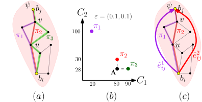
Figure 5: Introducing super-edges connecting the boundary vertices $b_{i}$ and $b_{j}$ in cluster $\psi$. See Example 1 for details.

5.2 Query Phase

Recall that in the query phase, we assume to have the graph $\mathcal{G}=(\mathcal{V},\mathcal{E})$ and the user-provided approximation factor $\boldsymbol{\varepsilon}$ as well the set of correlated clusters $\Psi$ generated during the preprocessing phase. Given a query $v_{\text{s}},v_{\text{t}}\in\mathcal{V}$ we wish to efficiently compute $\Pi^{*}_{\boldsymbol{\varepsilon}}(v_{\text{s}},v_{\text{t}})$.

We start by defining a new graph $\tilde{\mathcal{G}}$ which we call the query graph. $\tilde{\mathcal{G}}$, which will be implicitly constructed, contains super-edges that avoid having a search algorithm enter correlated clusters that do not include $v_{\text{s}}$ and $v_{\text{t}}$.

Each edge in the query graph will be associated with two cost functions which will induce a generalized query graph such that running GA*pex on this generalized query graph will allow us to efficiently compute $\Pi^{*}_{\boldsymbol{\varepsilon}}$.

Unfortunately, the branching factor of vertices in $\tilde{\mathcal{G}}$ may turn out to be quite large. Thus, we continue to describe how to use standard algorithmic practices to deal with it.

Query Graph

It will be convenient to assume that every vertex $v\in\mathcal{V}$ belongs to a correlated cluster. If $v$ was not assigned a cluster in the preprocessing phase, we will assign it with a trivial cluster $(\{v\},\emptyset,\ell_{v},\delta_{v})$ containing only $v$ and no edges and add the cluster to $\Psi$.

Let $\psi_{s}$ and $\psi_{t}$ denote the correlated clusters containing $v_{\text{s}}$ and $v_{\text{t}}$, respectively. We define the query graph $\tilde{\mathcal{G}}=(\tilde{\mathcal{V}},\tilde{\mathcal{E}})$ as follows:

$$\tilde{\mathcal{V}}=\underbrace{\left(V_{\psi_{s}},\cup\ V_{\psi_{t}}\right)}_{(\diamondsuit)}\cup\underbrace{\left(\cup_{\psi\in\Psi\setminus\{\psi_{s}\psi_{t}\}}B(\psi)\right)}_{(\heartsuit)},$$

$$\tilde{\mathcal{E}}=\underbrace{\left(\mathcal{E}\setminus\{E_{\psi}~|~\psi\in\Psi\setminus\{\psi_{s},\psi_{t}\}\}\right)}_{(\clubsuit)}\cup\underbrace{\left(\cup_{\psi\in\Psi\setminus\{\psi_{s},\psi_{t}\}}{\hat{\mathcal{E}}_{\psi}}\right)}_{(\spadesuit)}.$$

Namely, the vertices $\tilde{\mathcal{V}}$ include $(\diamondsuit)$ all vertices of clusters $\psi_{s}$ and $\psi_{t}$ and $(\heartsuit)$ all boundary vertices of the other clusters. The edges $\tilde{\mathcal{E}}$ include $(\clubsuit)$ all edges between clusters as well as all edges of clusters $\psi_{s}$ and $\psi_{t}$ and $(\spadesuit)$ all the super-edges of the clusters that are not $\psi_{s}$ and $\psi_{t}$.

We are now ready to define the generalized query graph $(\tilde{\mathcal{V}},\tilde{\mathcal{E}},\tilde{\mathbf{c}},\tilde{\mathbf{c}}^{\prime})$ corresponding to query graph. The only thing we need to describe are the edge costs functions $\tilde{\mathbf{c}}$ and $\tilde{\mathbf{c}}^{\prime}$. For each original edge $e\in\mathcal{E}$ we set $\tilde{\mathbf{c}}(e):=\mathbf{c}(e)$ and $\tilde{\mathbf{c}}^{\prime}(e):=\mathbf{c}(e)$. For each super-edge $\hat{e}\in\hat{\mathcal{E}}_{\psi}$ of cluster $\psi$ we set $\tilde{\mathbf{c}}(\hat{e}):=\mathbf{c}_{\psi}(\hat{e})$ and $\tilde{\mathbf{c}}^{\prime}(\hat{e}):=\mathbf{c}^{\prime}_{\psi}(\hat{e})$.

In the following example, we detail the part of the query graph corresponding to the correlated cluster depicted in Fig. 5 and the paths described in Example 1.

Example 2.

Consider the cluster $\psi$ detailed in Example 1 and assume that neither $v_{\text{s}}$ nor $v_{\text{t}}$ are in $V_{\psi}$. Let us consider the contribution of $\psi$ to the query graph $\tilde{\mathcal{G}}=(\mathcal{\tilde{V}},\mathcal{\tilde{E}})$. First, all boundary vertices of $\psi$ such as $b_{i}$ and $b_{j}$ will be added to $\mathcal{\tilde{V}}$ while internal vertices such as $u,v\in\mathcal{V}_{\psi}$ will not. Second, the super-edges of $\psi$ such as $\{\hat{e}^{1}_{ij},\hat{e}^{2}_{ij}\}$ are added to $\mathcal{\tilde{E}}$ as well as edges connecting boundary vertices of $\psi$ to vertices not in $\psi$. On the other hand, internal cluster’s edges, as $(u,v)$, are removed. Now, recall that before we can run GA*pex, we construct the generalized query graph $(\mathcal{\tilde{V}},\mathcal{\tilde{E}},\tilde{\mathbf{c}},\tilde{\mathbf{c}}^{\prime})$. For super-edges like $\hat{e}^{2}_{ij}\in\hat{\mathcal{E}}_{\psi}$, the costs will be $\tilde{\mathbf{c}}(\hat{e}^{2}_{ij})=\mathbf{c}_{\psi}(\hat{e}^{2}_{ij})=(80,30)$ and $\tilde{\mathbf{c}}^{\prime}(\hat{e}^{2}_{ij})=\mathbf{c}^{\prime}_{\psi}(\hat{e}^{2}_{ij})=(80,28)$.

Lemma 5.1.

For any correlated cluster $\psi$ and any two boundary vertices $b_{i},b_{j}\in B(\psi)$, the Pareto-optimal solution set $\Pi^{*}(b_{i},b_{j})$ in $(V_{\psi},E_{\psi},\mathbf{c}_{\psi})$ is an $\boldsymbol{\varepsilon}$-approximation set of the Pareto-optimal solution set $\Pi^{*}(b_{i},b_{j})$ in $(V_{\psi},E_{\psi},\mathbf{c^{\prime}}_{\psi})$.

We omit the proof of the lemma. The following theorem, stated without proof, summarizes the correctness of the generalized query graph construction.

Theorem 5.2.

Let $v_{\text{s}}$ and $v_{\text{t}}$ be the start and target vertices, respectively, of a search query. Running GA*pex on the generalized query graph yields an $\boldsymbol{\varepsilon}$-approximation of $\Pi^{*}$ in $\mathcal{G}$.

Lazy Edge Expansion

Recall that within a correlated cluster $\psi$, we connect all pairs of boundary vertices $b_{i},b_{j}\in~B(\psi)$ by one or more super-edges of the set $\hat{\mathcal{E}}_{\psi,i,j}$. Namely, the number of super-edges introduced is at least quadratic in the number of boundary vertices. Thus, the branching factor of $\tilde{\mathcal{G}}$ may dramatically increase. Unfortunately, large branching factors are known to dramatically slow down search-based algorithms (even single-objective ones) (Korf 1985; Edelkamp and Korf 1998).

To this end, we endow our search algorithm with a lazy edge-expansion strategy (Yoshizumi, Miura, and Ishida 2000) for the super-edges. Specifically, we maintain two edge lists for each vertex: regular edges and super-edges, both ordered lexicographically from low to high using the edge’s $\mathbb{f}$-value. When expanding a node, all successors derived from regular edges are pushed to Open as before. For super-edges, however, we follow a partial expansion approach: we iterate over super-edges in increasing lexicographic $\mathbb{f}$-value order and stop as soon as the first successor (originating from a super-edge) is inserted into Open. When a boundary vertex is popped from Open, we expand the next-best super-edge of its predecessor. I.e., the next unprocessed super-edge from the super-edges list of the predecessor. We refer to the adaptation of GA*pex as described above as Partial Expansion GA*pex (PE-GA*pex).

6 Evaluation

We implemented our algorithms using a combination of Python and C++. We ran all experiments on an HP ProBook 440 G8 Notebook with 16GB of memory. The A*pex and PE-GA*pex algorithms were implemented based on A*pex original C++ implementation. All experiments were executed on the NY, COL, NW and CAL DIMACS instances, which contain between 250K and 1.9M vertices.

As an optimization step for the ICCA process (Q2, Sec. 5.1), we employed a simple and efficient method for approximating $\Pi^{*}(b_{i},b_{j})$ without calling A*pex (as described in Sec. 5.1). Specifically, we ran two single-objective Dijkstra shortest-path queries, one for each objective, for the query $b_{i}\rightarrow b_{j}$ considering only the subgraph of cluster $\psi$. We then checked if the user-provided approximation factors is sufficient for $\boldsymbol{\varepsilon}$-dominating $\Pi^{*}(b_{i},b_{j})$ with a single solution. If so, this solution was used to obtain $\hat{\mathcal{E}}_{\psi,i,j}$. This straightforward step is usually one to two orders of magnitude faster than running A*pex directly.

6.1 Correlation-Based Preprocessing on DIMACS

Instance	$|\mathcal{V}|$	$|\tilde{\mathcal{V}}|$	$|\mathcal{E}|$	$|\tilde{\mathcal{E}}|$	$b(\mathcal{G})$	$b(\tilde{\mathcal{G}})$	Time [sec]	Space [GB]
NY	$26$	$4.3$	$73$	$110$	$2.8$	$25.7$	$39$	$0.5$
COL	$43$	$8.2$	$106$	$93$	$2.4$	$11.2$	$47$	$0.5$
NW	$121$	$18$	$284$	$227$	$2.4$	$12.7$	$127$	$0.9$
CAL	$189$	$25$	$466$	$360$	$2.5$	$14.3$	$208$	$1.7$

Table 1: Comparison of the size of $\mathcal{G}$ (original graph) and $\tilde{\mathcal{G}}$ (query graph) for $\boldsymbol{\varepsilon}=[0.01,0.01]$, including the number of vertices and edges (in tens of thousands), average branching factor $b$, and preprocessing time and space usage.

Recall that the DIMACS dataset is a standard benchmark in the field and is supposed to simulate real-world data. Thus, we start by reporting how our framework behaves on this dataset. Tbl. 1 compares the original graph $\mathcal{G}$ and the query graph $\tilde{\mathcal{G}}$ in terms of size (vertices, edges, average branching factor), as well as preprocessing time and space required for storing the optimal paths abstracted by super-edges. As expected, $\tilde{\mathcal{G}}$ consistently has dramatically fewer vertices but a higher branching factor when compared to $\mathcal{G}$. However, these two factors counterbalance each other, and both graphs have comparable number of edges.

We continue to visualize the objective correlation and how it manifests in our framework for the NY and CAL DIMACS instances. Plotting the edge costs as points in the bi-objective space (Fig. 7a,7c), we can see that the entire bi-objective space can be decomposed into four disjoint, highly-correlated linear relationships—a pattern observed consistently across the DIMACS dataset. These four modes of correlation were detected by the RANSAC method (Alg. 1). Importantly, each mode needs to be further subdivided into correlated clusters which are depicted in Fig. 7b,7d.

6.2 Lazy Edge Expansion Ablation Study

As demonstrated in Sec. 6.1, $\tilde{\mathcal{G}}$’s branching factor is much larger than $\mathcal{G}$’s which is why we suggested a lazy edge-expansion strategy (Sec. 5.2). To this end, we compare (Fig. 6(a)) the query execution times of GA*pex and PE-GA*pex on $\tilde{\mathcal{G}}$, across various DIMACS instances for an approximation factor of $\boldsymbol{\varepsilon}=[0.01,0.01]$. PE-GA*pex outperforms GA*pex for almost all instances with the speed up in query times reaching above $5\times$.

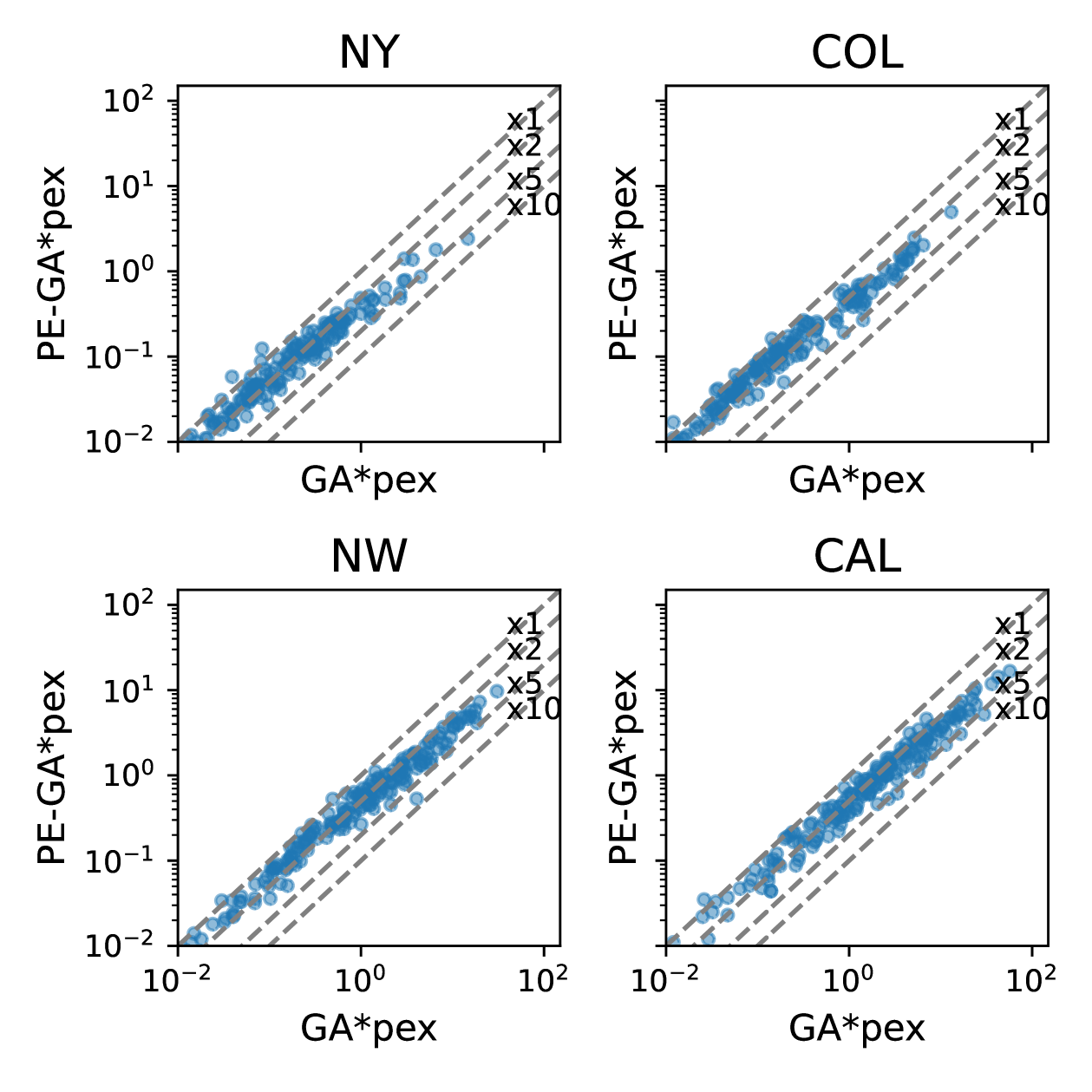
(a)

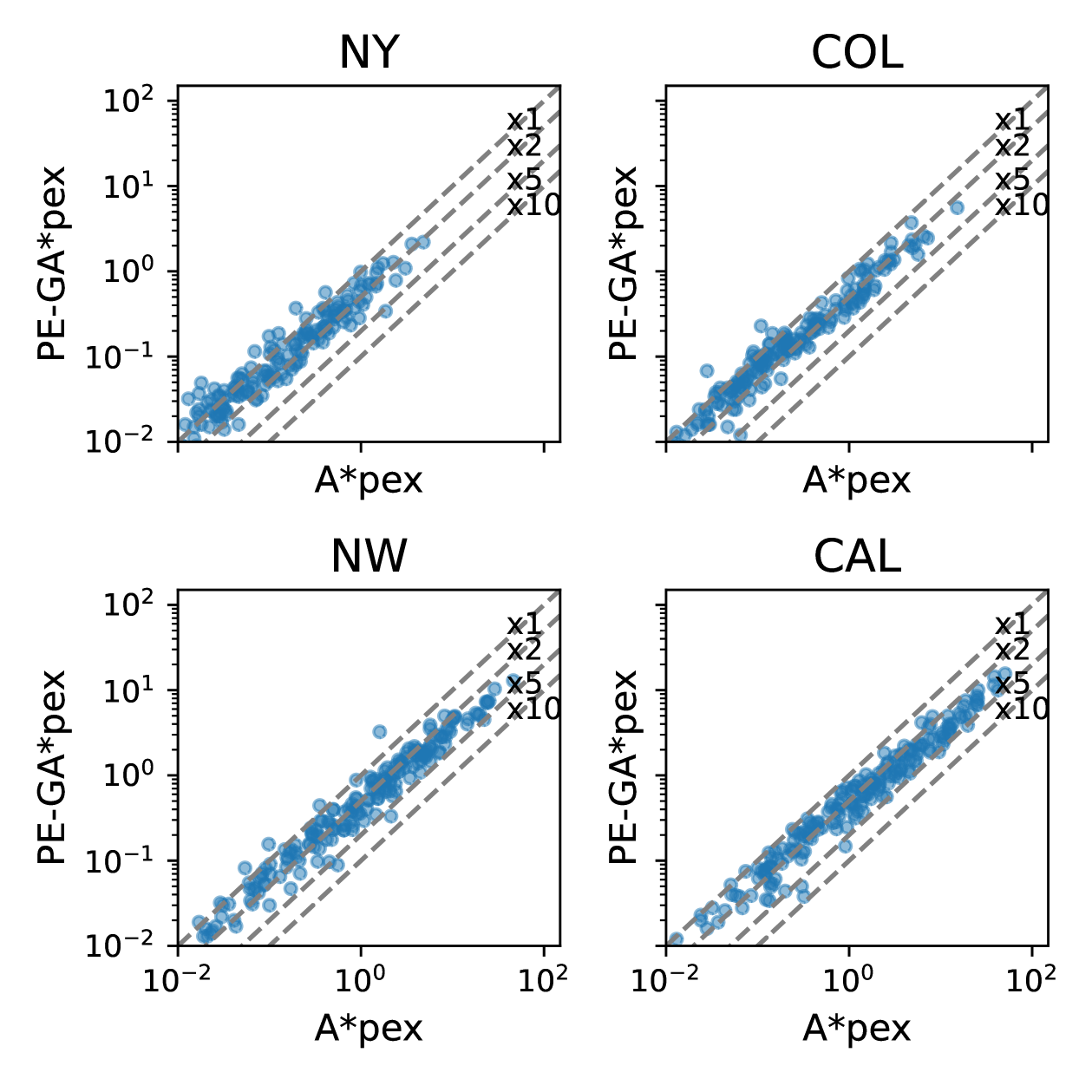
(b)

Figure 6: Running times (in seconds) on different queries and DIMACS instances for $\boldsymbol{\varepsilon}=[0.01,0.01]$. (a) Ablation study—comparing PE-GA*pex with GA*pex. (b) Approach evaluation—comparing PE-GA*pex with A*pex.

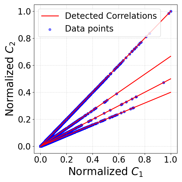
(a)

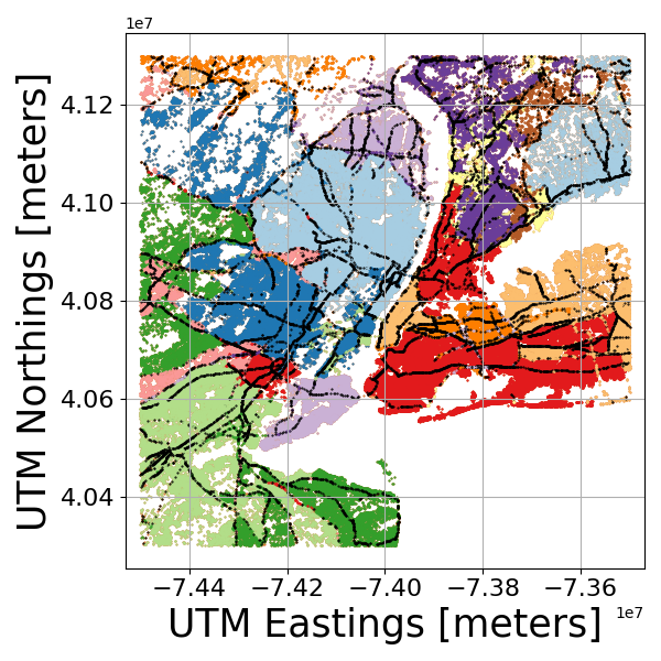
(b)

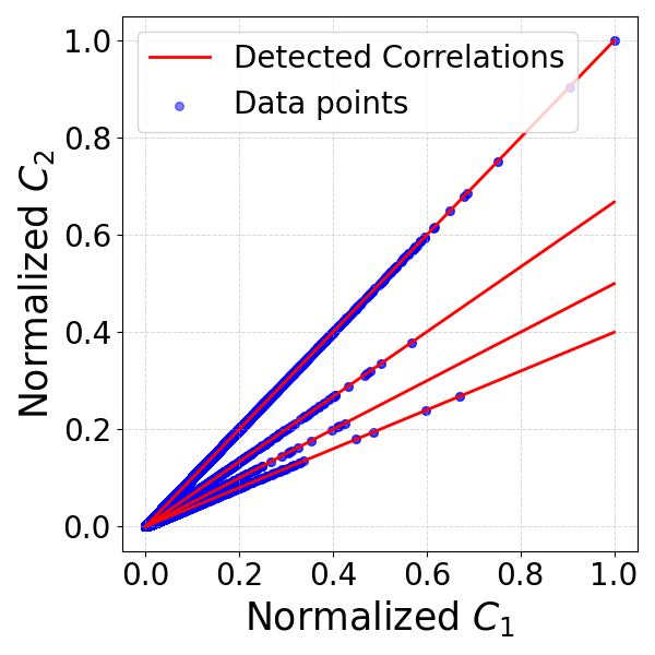
(c)

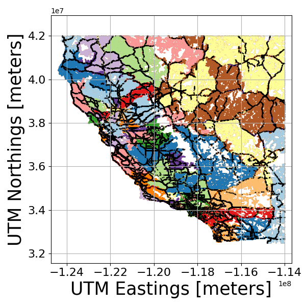
(d)

Figure 7: (a)+(c) Edge cost plotted on the 2D objective costs (blue dots) and linear correlations computed by Alg.1 (red lines) for the NY and CAL instances, respectively. (b)+(d) Geo-spatial display of NY’s and CAL’s correlated clusters (plotted as color patches), respectively, computed using the correlation clustering method (Sec. 5.1). Each cluster’s boundary vertices are marked in black dots.

6.3 PE-GA*pex Query Runtimes

We compare query running times of PE-GA*pex and A*pex, arguably the state-of-the-art algorithm for solving the approximate BOSP problem (without preprocessing) on various DIMACS roadmaps. We tested both on the highly-correlated DIMACS instances (Sec. 6.1) and then continue to generate a synthetic instances in which we took the DIMACS NY instance and randomly sampled edges costs to form three linear non-perfect correlations (Fig. 8(a)).

For the highly-correlated DIMACS instances, other than a small number of outliers, PE-GA*pex is always faster than A*pex with maximal speed ups being well above $5\times$ (Fig. 6(b)). For the synthetic NY-based instance, we preprocessed the graph using a fixed value of $\delta=0.05$ and four approximation factors $\boldsymbol{\varepsilon}~=~\bigl{\{}[0.001,0.001],[0.005,0.005],[0.01,0.01],[0.1,0.1]\bigr{\}}$. This combination of $\delta$ and $\boldsymbol{\varepsilon}$ keeps the number of vertices of $\tilde{\mathcal{G}}$ fixed while the average branching factor $b(\tilde{\mathcal{G}})$ increases as $\boldsymbol{\varepsilon}$-values decrease. Again, we compare query running times of PE-GA*pex and A*pex and can see (Fig. 8(b)) a dramatic speed up on most queries, reaching, in some instances, up to $1000\times$.

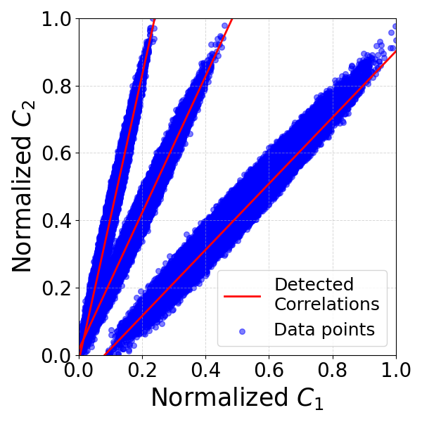
(a)

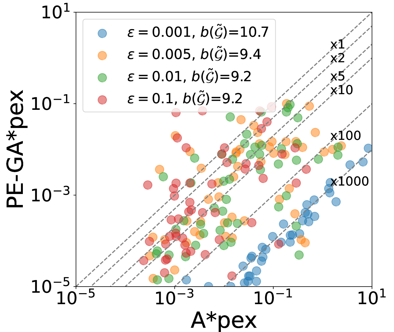
(b)

Figure 8: (a) Edge cost plotted on the 2D objective costs (blue dots) and linear correlations computed by Alg.1 (red lines) for the synthetic bi-objective graph. (b) Running times (in seconds) of A*pex and PE-GA*pex on different queries in a synthetic bi-objective graph for varying $\boldsymbol{\varepsilon}$ vectors.

7 Discussion and Future Work

In this work we presented the first practical, systematic approach to exploit correlation between objectives in BOSP. Our approach is based on a generalization to A*pex that is of independent interest and an immediate question is what other problems can make use of this new algorithmic building block. Our empirical evaluation on standard DIMACS benchmarks (Sec. 6) indicate that costs of edges in instances of this dataset follow a nearly-perfect correlation (Fig. 7(c)). Thus, this dataset may be too synthetic to represent real-world data and better benchmarks are in need (a gap already identified by Salzman et al. (2023)).

As for future work, in our framework we introduce $\delta$ to control which edges are considered to have the same correlation. This parameter is intimately related to the approximation factor $\boldsymbol{\varepsilon}$. Automatically choosing $\delta$ according to a given value of $\boldsymbol{\varepsilon}$ would reduce the algorithm’s parameters.

One other avenue for future work includes extending our framework to more than two objectives. This is highly challenging, as the number of correlated objectives may vary across different parts of the graph. Finally, it is extremely interesting to integrate our approach within the contraction hierarchies-based framework recently proposed by Zhang et al. (2023b) for exact BOSP problems.

References

- Breugem, Dollevoet, and van den Heuvel (2017) Breugem, T.; Dollevoet, T.; and van den Heuvel, W. 2017. Analysis of FPTASes for the multi-objective shortest path problem. Computers & Operations Research, 78: 44–58.
- Brumbaugh-Smith and Shier (1989) Brumbaugh-Smith, J.; and Shier, D. 1989. An empirical investigation of some bicriterion shortest path algorithms. European Journal of Operational Research, 43(2): 216–224.
- Edelkamp and Korf (1998) Edelkamp, S.; and Korf, R. E. 1998. The branching factor of regular search spaces. In Association for the Advancement of Artificial Intelligence (AAAI), 299–304.
- Ehrgott (2005) Ehrgott, M. 2005. Multicriteria optimization, volume 491. Springer Science & Business Media.
- Fischler and Bolles (1981) Fischler, M. A.; and Bolles, R. C. 1981. Random sample consensus: a paradigm for model fitting with applications to image analysis and automated cartography. Communications of the ACM, 24(6): 381–395.
- Fu et al. (2023) Fu, M.; Kuntz, A.; Salzman, O.; and Alterovitz, R. 2023. Asymptotically optimal inspection planning via efficient near-optimal search on sampled roadmaps. Int. J. Robotics Res., 42(4-5): 150–175.
- Goldin and Salzman (2021) Goldin, B.; and Salzman, O. 2021. Approximate bi-criteria search by efficient representation of subsets of the pareto-optimal frontier. In International Conference on Automated Planning and Scheduling (ICAPS), volume 31, 149–158.
- Hernández et al. (2023) Hernández, C.; Yeoh, W.; Baier, J. A.; Zhang, H.; Suazo, L.; Koenig, S.; and Salzman, O. 2023. Simple and efficient bi-objective search algorithms via fast dominance checks. Artificial intelligence, 314: 103807.
- Korf (1985) Korf, R. E. 1985. Depth-first iterative-deepening: An optimal admissible tree search. Artificial intelligence, 27(1): 97–109.
- Mahmood, Han, and Lee (2020) Mahmood, B.; Han, S.; and Lee, D.-E. 2020. BIM-based registration and localization of 3D point clouds of indoor scenes using geometric features for augmented reality. Remote Sensing, 12(14): 2302.
- Mandow and De La Cruz (2008) Mandow, L.; and De La Cruz, J. L. P. 2008. Multiobjective A* search with consistent heuristics. Journal of the ACM (JACM), 57(5): 1–25.
- Mote, Murthy, and Olson (1991) Mote, J.; Murthy, I.; and Olson, D. L. 1991. A parametric approach to solving bicriterion shortest path problems. European Journal of Operational Research, 53(1): 81–92.
- Pearson (1895) Pearson, K. 1895. VII. Note on regression and inheritance in the case of two parents. Proceedings of the royal society of London, 58(347-352): 240–242.
- Perny and Spanjaard (2008) Perny, P.; and Spanjaard, O. 2008. Near admissible algorithms for multiobjective search. In European Conference on Artificial Intelligence (ECAI), 490–494. IOS Press.
- Pulido, Mandow, and Pérez-de-la Cruz (2015) Pulido, F.-J.; Mandow, L.; and Pérez-de-la Cruz, J.-L. 2015. Dimensionality reduction in multiobjective shortest path search. Computers & Operations Research, 64: 60–70.
- Ren et al. (2025) Ren, Z.; Hernández, C.; Likhachev, M.; Felner, A.; Koenig, S.; Salzman, O.; Rathinam, S.; and Choset, H. 2025. EMOA*: A framework for search-based multi-objective path planning. Artificial Intelligence, 339: 104260.
- Salzman et al. (2023) Salzman, O.; Felner, A.; Zhang, H.; Chan, S.-H.; and Koenig, S. 2023. Heuristic-Search Approaches for the Multi-Objective Shortest-Path Problem: Progress and Research Opportunities [Survey Track]. In International Joint Conferences on Artificial Intelligence (IJCAI).
- Skriver et al. (2000) Skriver, A. J.; et al. 2000. A classification of bicriterion shortest path (BSP) algorithms. Asia Pacific Journal of Operational Research, 17(2): 199–212.
- Skyler et al. (2022) Skyler, S.; Atzmon, D.; Felner, A.; Salzman, O.; Zhang, H.; Koenig, S.; Yeoh, W.; and Ulloa, C. H. 2022. Bounded-cost bi-objective heuristic search. In Symposium on Combinatorial Search (SoCS), volume 15, 239–243.
- Stewart and White III (1991) Stewart, B. S.; and White III, C. C. 1991. Multiobjective a. Journal of the ACM (JACM), 38(4): 775–814.
- Tarapata (2007) Tarapata, Z. 2007. Selected multicriteria shortest path problems: An analysis of complexity, models and adaptation of standard algorithms. International Journal of Applied Mathematics and Computer Science, 17(2): 269–287.
- Tarjan (1972) Tarjan, R. 1972. Depth-first search and linear graph algorithms. SIAM Journal on Computing (SICOMP), 1(2): 146–160.
- Tsaggouris and Zaroliagis (2009) Tsaggouris, G.; and Zaroliagis, C. 2009. Multiobjective optimization: Improved FPTAS for shortest paths and non-linear objectives with applications. Theory of Computing Systems, 45(1): 162–186.
- Ulungu and Teghem (1994) Ulungu, E. L.; and Teghem, J. 1994. Multi-objective combinatorial optimization problems: A survey. Journal of Multi-Criteria Decision Analysis, 3(2): 83–104.
- Verel et al. (2013) Verel, S.; Liefooghe, A.; Jourdan, L.; and Dhaenens, C. 2013. On the structure of multiobjective combinatorial search space: MNK-landscapes with correlated objectives. European Journal of Operational Research, 227(2): 331–342.
- Yoshizumi, Miura, and Ishida (2000) Yoshizumi, T.; Miura, T.; and Ishida, T. 2000. A* with Partial Expansion for Large Branching Factor Problems. In Association for the Advancement of Artificial Intelligence (AAAI), 923–929.
- Zhang et al. (2024a) Zhang, H.; Salzman, O.; Felner, A.; Kumar, T. K. S.; and Koenig, S. 2024a. Bounded-Suboptimal Weight-Constrained Shortest-Path Search via Efficient Representation of Paths. In International Conference on Automated Planning and Scheduling (ICAPS), 680–688.
- Zhang et al. (2023a) Zhang, H.; Salzman, O.; Felner, A.; Kumar, T. K. S.; Skyler, S.; Ulloa, C. H.; and Koenig, S. 2023a. Towards Effective Multi-Valued Heuristics for Bi-objective Shortest-Path Algorithms via Differential Heuristics. In Symposium on Combinatorial Search (SoCS), 101–109.
- Zhang et al. (2023b) Zhang, H.; Salzman, O.; Felner, A.; Kumar, T. S.; Ulloa, C. H.; and Koenig, S. 2023b. Efficient multi-query bi-objective search via contraction hierarchies. In International Conference on Automated Planning and Scheduling (ICAPS), volume 33, 452–461.
- Zhang et al. (2024b) Zhang, H.; Salzman, O.; Felner, A.; Ulloa, C. H.; and Koenig, S. 2024b. A-A*pex: Efficient Anytime Approximate Multi-Objective Search. In Symposium on Combinatorial Search (SoCS), 179–187.
- Zhang et al. (2022) Zhang, H.; Salzman, O.; Kumar, T. S.; Felner, A.; Ulloa, C. H.; and Koenig, S. 2022. A*pex: Efficient approximate multi-objective search on graphs. In International Conference on Automated Planning and Scheduling (ICAPS), volume 32, 394–403.