Reconfigurable Defect States in Non-Hermitian Topolectrical Chains with Gain and Loss
Abstract
We investigate the interplay between the non-Hermitian skin effect (NHSE), parity-time (PT) symmetry, and topological defect states in a finite non-Hermitian Su-Schrieffer-Heeger (SSH) chain. In the conventional NHSE regime, non-reciprocal hopping leads to an asymmetric localization of all eigenstates at one edge of the system, including the bulk and topological edge states. However, the introduction of staggered gain and loss restores the symmetric localization of topological edge states while preserving the bulk NHSE. We further examine the response of defect states in this system, demonstrating that their spatial localization is dynamically controlled by the combined effects of NHSE and PT symmetry. Specifically, we identify three distinct regimes in which the defect states localize at the defect site, shift to the system’s edges, or become completely delocalized. These findings extend beyond previous works that primarily explored the activation and suppression of defect states through gain-loss engineering. To validate our theoretical predictions, we propose an experimental realization using a topolectrical circuit, where non-Hermitian parameters are implemented via impedance converter-based non-reciprocal elements. Circuit simulations confirm the emergence and tunability of defect states through voltage and admittance measurements, providing a feasible platform for experimental studies of non-Hermitian defect engineering. Our results establish a route for designing reconfigurable non-Hermitian systems with controllable topological defect states, with potential applications in robust signal processing and sensing.
I Introduction
In recent years, non-Hermitian systems [1, 2, 3, 4, 5, 6, 7, 8] have attracted significant attention owing to their unique properties and potential applications in various fields such as photonics [9, 10, 11], condensed matter physics [12, 13, 14, 15], and quantum computing [16, 17, 18, 19]. These systems have complex eigenvalues and non-orthogonal eigenvectors, making them fundamentally different from their Hermitian counterparts [20, 21, 22, 23].
One intriguing phenomenon in non-Hermitian systems is the non-Hermitian skin effect (NHSE) [24, 25, 4, 26, 27, 28, 29, 30], which refers to the localization of bulk states near the boundaries of the system. The NHSE has been observed in various non-Hermitian systems such as non-Hermitian photonic lattices [31, 32, 33], topolectrical (TE) circuits [34, 35, 36, 37, 38, 39, 40, 41, 42, 43, 44, 45], non-Hermitian topological insulators [46, 47, 48, 49, 50], and non-Hermitian quantum systems [30, 51, 52].
Topological edge states are a hallmark of topological phases of matter [53, 54, 55, 56, 40, 57, 58], and have been extensively studied in Hermitian systems. In recent years, the study of topological edge states has been extended to non-Hermitian systems [59, 60]. The coexistence of topological edge states and NHSE in non-Hermitian systems has been shown to lead to novel phenomena, such as the selective enhancement of topological zero modes [61]. Another intriguing feature of non-Hermitian systems is the existence of topological defect states [62, 63, 61, 64, 65, 66, 67, 68, 69], which are localized states that appear at the interface of two regions with different topological properties. These states have been studied in various non-Hermitian systems, such as non-Hermitian photonic lattices [70] and non-Hermitian topological insulators [68]. Recently, Stegmaier et al. (Ref. 68) demonstrated the critical role of system symmetry in the emergence of defect states within a configuration comprising two non-Hermitian chains, each characterized by staggered gain/loss terms and connected via a central defect site. Specifically, they revealed that defect states are present when the system exhibits parity-time (PT) and anti-PT (APT) symmetries, but are absent under conditions of broken-PT (BPT) symmetry. However, the model employed by Stegmaier et al. did not incorporate any coupling asymmetry within the chain. Consequently, the interplay between defect states, topological edge states and the localization effects attributed to NHSE, remained unexplored.
In this paper, we investigate the effect of the NHSE on the localization properties of defect and edge states in non-Hermitian systems. We show that the NHSE drags not only the bulk states but also the edge states towards the boundary, resulting in the localization of both types of eigenstates near the boundary. We further explore the possibility of enhancing the localization properties of the edge states by introducing staggered gain and loss potential to the sublattice sites. This results in the superimposition of the NHSE and edge state localization at opposite edges.
We further analyze the effect of the gain/loss term on defect states. We introduce balanced gain/loss terms on the A/B sublattice sites of a Su-Schrieffer-Heeger (SSH) chain while leaving the defect states passive. By modulating the gain/loss terms, we observe different types of eigenstates and localization properties depending on the PT symmetry of the system. Interestingly, we find that defect states appear only in the PT- and APT-symmetric cases and are suppressed in the broken PT-symmetric case. We explain analytically the observed correlation between the emergence and localization of the defect states and the PT symmetry. Additionally, we propose an experimental realization of our model using a non-hermitian TE circuit. This circuit design validates our theoretical predictions through its electrical characteristics, such as voltage and admittance responses, by demonstrating the presence and control of defect states via non-Hermitian parameters. The capability to switch topological defect states and adjust their localization has significant implications for defect engineering in non-Hermitian systems.
II Characteristics of pristine non-Hermitian SSH chain with loss and gain
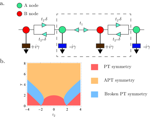
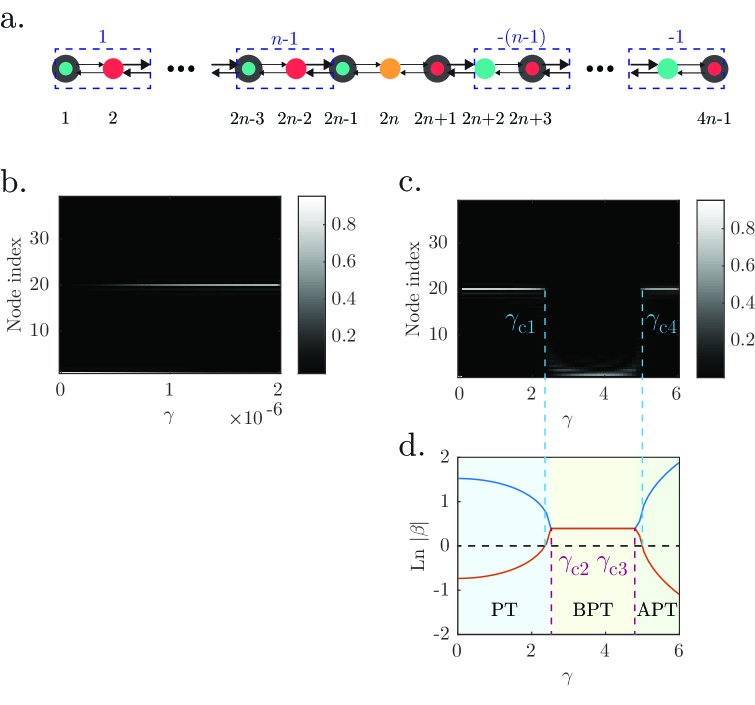
We investigate the emergence of the NHSE and topological edge states in a generic one-dimensional lattice model with two sublattice nodes denoted as A and B nodes (refer to Fig. 1a). Specifically, we focus on a modified non-Hermitian SSH chain with reciprocal intra-chain () and non-reciprocal inter-chain () coupling in which gain () and loss () are present at the A and B nodes, respectively. Under periodic conditions, the Bloch Hamiltonian of the system is given by
| (1) |
where is the th Pauli matrix, and denote the intra- and inter-cell couplings, respectively, and the degree of non-reciprocity in the inter-unit cell couplings, which may be achieved, for example, via the use of negative impedance converters at current inversion (INICs) in a TE realization [44, 71, 43, 38]. As above-mentioned, represents the staggered gain and loss terms. The corresponding eigenvalues are given by
| (2) |
Unless otherwise stated, we assume the case where and that . All the eigenenergies of the bulk states in a finite open chain are real when , which corresponds to the PT-symmetric case. However, at large values of the gain/loss term, i.e., , the eigenenergies become imaginary in the anti PT-symmetric phase. At intermediate values of at which , the eigenvalue spectrum contains a mixture of real and imaginary eigenenergies, which is referred to as the broken PT-symmetric case. These three phases are delineated in the phase diagram drawn in Fig. 1b.
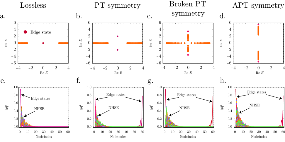
We analyze the evolution of the edge and NHSE states for the three different PT symmetry cases by plotting the complex eigenenergy and eigenstate spatial distributions under varying gain/loss strengths in Fig. 2.
We first consider the case with . The Hamiltonian in Eq. (1) exhibits a chiral symmetry, i.e., with . The chiral symmetry protects the topologically nontrivial states, which are characterized by a winding number. One way to calculate this winding number is to convert Eq. (1) into a Hermitian form via a similarity transform as described below.
In the absence of the loss/gain term (i.e. ), the Hamiltonian in Eq. (1) under OBC can be written in the real space basis as
| (3) |
where is the basis state for the th unit cell, is the basis state for the A / Bth sublattice, and . can be converted into a Hermitian Hamiltonian via a similarity transformation operator :
| (4) |
where
| (5) |
and
| (6) |
| (7) |
It can be seen by a direct comparison of Eqs. (3) and (5) that in the latter corresponds to in the former (in other words, the interchain coupling of is replaced by the . In the original SSH chain with gain/loss but without coupling asymmetry (i.e., ), we can obtain the completely real or imaginary eigenspectrum if and , respectively. Hence, for the non-Hermitian SSH chain if we replace the by the , the condition for entirely real and complex eigenspectrum is then given by and , respectively). Eqs. (3) and (5) share the same eigenvalues while their corresponding eigenvectors are scaled relative to each other by an exponential factor of . A consequence of this is that topological phase of the non-Hermitian Hamiltonian in Eq. (3) can be predicted by calculating the winding number of its Hermitian counterpart in Eq. (5). This winding number is given by
| (8) |
For the case where the winding number is nonzero, two topological zero-energy edge states appear in the complex energy spectrum (see Fig. 2a where the two degenerate edge states occur at .). The asymmetry in the inter-chain couplings results in the exponential localization of all the eigenstates, which is a direct consequence of NHSE (see Fig. 2e-h). For a bulk state, this exponential accumulation arises from the shift of wavevector from a real value, under PBC to a complex value of under OBC, where is the inverse decay length related to the non-Bloch factor, which is given by , .
In Fig. 2, the given system parameters yield a value in the range , which results in all bulk states to be localized at the left edge (Figs. 2e-h). It is worth noting that the NHSE causes both of the topological edge states to be displaced towards the preferred edge (i.e., the left edge in the case depicted by Fig. 2e) when . This behavior is different from the Hermitian case where the two edge states are localized at two opposite ends [72]. In contrast, a non-zero restores the localization of the edge states to the two end nodes (Figs. 2f-h) seen in the Hermitian case. The restoration is independent of the NHSE localization of the bulk states remains largely unchanged by the insertion of the gain/loss term. Additionally, the alternating gain/loss term does not significantly affect the decay lengths of the bulk or topological edge states (Fig. 2f-h). Therefore, one can surmise that it is the presence of onsite gain/loss potential rather than its sign which causes one of the topological edge states to be spatially separated from the NHSE localized bulk states.
We will now analytically explain the observed behavior of the topological edge states by considering the concept of the edge Hamiltonian. For a finite system of unit cells described by the Hermitian Hamiltonian , the edge Hamiltonian is constructed by projecting into the basis of ,which correspond to the normalized wavefunctions at the first unit cells of the edge states for semi-infinite systems localized along the left and right edges truncated to unit cells. Explicitly, the basis states are given by
| (9) | ||||
| (10) |
where
| (11) |
are normalization factors introduced so that , and the unit cells are numbered from 0 to . When , is then given by
| (12) |
The eigenvalues of , , are then approximately the eigenenergies of the topological edge states of Eq. (5) while its eigenvectors would approximate the corresponding wavefunctions of the edge states. Note that the similarity transformation of Eq. (4) implies that if is an eigenstate of , then is an eigenstate of . By using the fact that where is defined in Eq. (6) and are defined in Eqs. (9) and (10), respectively, is then given by
| (13) |
Depending on the signs of and , the corresponding topological edge state may be localized at the left (right) edge for positive (negative) values of the logarithm. For the parameter set in Fig. 2e, both of the topological edge states are localized at the left edge.
We now include the finite gain / loss term, i.e., the Hamiltonian is modified as
| (14) |
Projecting the above into the basis of , we obtain
| (15) | ||||
| (16) |
It can be observed from the definitions of in Eq. (11) that as , and . The ratio of the magnitude of the term relative to that of the term therefore becomes smaller as the system size increases, and the eigenvalues of Eq. (16) , which correspond to the eigenenergies of the edge states, switch from real to imaginary and approach . This trend can be observed in Fig. 2b to Fig. 2d. Moreover, in the limit of large , the eigenvectors of Eq. (16) approach where and take the explicit forms of
| (17) | ||||
| (18) |
Under our assumptions of and , the factor of in has a magnitude that is larger than 1, which implies that with an eigenenergy near will be localized along the right edge. If , then , which has an eigenenergy of approximately ,will be localized along the left edge opposite from . Thus, under this condition, the introduction of a finite gain / loss term will result in the recovery of the conventional topological edge state configuration, i.e., with the two edge states localized at opposite edges of a sufficiently large system, as seen in Figs. 2f – g.
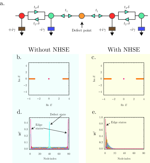
Now, we investigate the interplay between non-Hermiticity and topological defect states by studying a finite SSH chain with a defective node (indicated by the orange circle) that disrupts the alternating series of and couplings between neighboring nodes (refer to Fig. 3a). For a start, we assume there is no gain/loss term. We plot the corresponding eigenvalue and eigenstate distributions both with and without non-Hermiticity in Fig. 3b-e.
In the absence of non-Hermiticity (i.e., ), we observe zero-energy edge and defect states, as shown in Fig. 3b. These defect states are localized at the defective node, and there are two edge states in the eigenstate distribution, which are respectively localized at the two edges as shown in Fig. 3d. We then insert a finite non-Hermiticity into the system by setting the non-reciprocity factor to a finite value. Interestingly, although the eigenenergy spectrum remains largely unchanged (compare Fig. 3b with Fig. 3c), the defect states either vanish or move to one of the edges along with all of the bulk states which comprise of the NHSE localization (see Fig. 3e). Additionally, one of the topological edge states also shift to the other edge, joining the other edge state, as well as defect and bulk states localized there. Consequently, one can control the emergence and disappearance of the topological defect states merely by turning on or off the non-Hermiticity of the system.
Note that, in the homogenous state without defect, the left and right edge states are degenerate, and they will be dragged to the preferred side of NHSE. However, if the degeneracy of the left and right edge states are broken, the edge states will not be dragged by the NHSE, contrary to conventional expectations. As discussed in details in the next section, the breaking of degeneracy may occur in a heterojunction system with defect states and gain/loss potentials corresponding to different PT symmetries (symmetric, antisymmetric and broken). Additionally, we also note that the NHSE leads to the localization of all states towards the preferred edge only if there is matching non-Hermitian coupling asymmetry parameter across the defect states. Conversely, if the decay length of the non-Hermitian bulk states on either side of the defect states is unequal, the bulk states experiencing NHSE in the two segments will not converge to one edge by crossing the defect states.
III Effect of gain/loss on the defect states
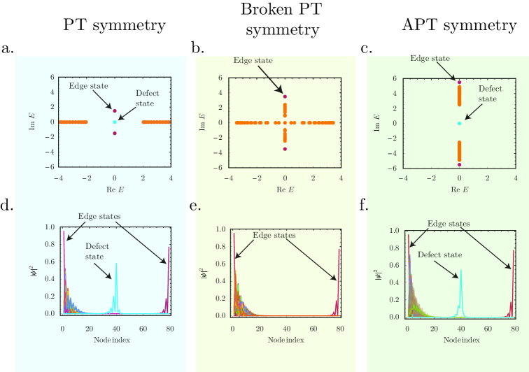
We now investigate the effect of gain/loss terms on the characteristics of the defect states [73, 74]. To do so, we add a balanced gain/loss term to the nodes respectively, while leaving the defect node passive, as shown in Fig. 3a. As before, by varying the factor, we can realize all three PT symmetries, i.e., the PT-symmetric, BPT-symmetric, and APT-symmetric cases, the eigenspectra of which are depicted in Figs. 4a to 4c, respectively. Interestingly, in the presence of a finite , defect states survive only in the PT- and APT-symmetric cases (see Fig. 4d,f), but are absent in the broken PT-symmetric case (see Fig. 4e). Energy-wise, the defect states are located at , while the edge states are located at . In all cases, we simultaneously observe both the NHSE and topological edge state localization.
To explain these observations in detail, we adopt the labeling scheme in Fig. 5a for a finite open chain containing complete unit cells (i.e., a pair of A and B-sublattice nodes) on either side of the three nodes comprising the defect and its immediate neighbors. We number the unit cells from 1 to for the unit cells to the left of the defect, and from to -1 for the unit cells on the right of the defect (blue labels above the chain in Fig. 5a). We concurrently number the individual nodes in the chain from 1 to (black labels below the chain in Fig. 5a).
Denoting the state of the entire chain as , we write the wavefunction of the th complete unit cell on the left of the defect as where ranges from 1 to , that of the th complete unit cell on the right of the defect as where to -1, and similarly that of the th individual node as . Note then that in this labeling scheme, , and , as indicated in Fig. 5a.
At , Eq. (3) for a periodic system can be written in the Bloch matrix form as
| (19) |
We observe from our numerical results that when defect states do exist in the defective chain, these defect states are pinned at the eigenenergy of [75]. We therefore focus on the zero-energy eigenstates. Eq. 19 admits two zero-energy eigenvectors, one of which is at and the other one of which is at where the superscript refers to the case here. The wavefunctions at the th unit cell to the left and right of the defect can thus be written as
| (20) | ||||
| (21) |
where is an unknown weight to be solved for.
Notice that () satisfies the boundary condition that the wavefunction must vanish at the node immediately to the left (right) of the leftmost (rightmost) node of the chain, i.e., (). To obtain the complete wavefunction of the chain, we apply the condition that the wavefunction must satisfy the Schroedinger equation at , , and which leads to the following equations:
| (22) | ||||
| (23) | ||||
| (24) |
Recalling that and (refer to Fig. 5a) and using the definitions of in Eqs. (20) and (21), the solution of Eqs. 22 to 24 yields
| (25) | ||||
| (26) | ||||
| (27) | ||||
| (28) | ||||
| (29) |
These expressions imply that at , only alternating nodes starting from the leftmost node in the chain have finite probability densities, as denoted by the thick black boundaries around these nodes in Fig. 5a. The defect node here serves as a transition point between the unit cells to its left, in which only the A sublattice nodes have finite probability densities, and the unit cells to its right, in which only the B sublattice nodes have finite probability densities. In particular, from Eqs. (25) and (29), the wavefunctions at the leftmost node and rightmost node are given by
| (30) | ||||
| (31) |
For and having an opposite sign to , as is the case here, the pre-factor of in implies that leading to eigenstate localization on the left edge of the chain, as shown in Figs. 3e and 5b.
When has a finite value, the zero-energy eigenvectors of become at and at where and, for ,
| (32) | ||||
| (33) |
Notice that the s are proportional to and vanish when .
To satisfy the boundary conditions that the wavefunction must vanish at the node immediately to the left of the leftmost node of the chain (i.e., ) and at the node immediately to the right of the rightmost node of the chain (i.e., ), assume the forms of
| (34) | |||
| (35) |
It can then be seen that the wavefunctions two nodes to the left () of the defect and two nodes to the right of the defect () are respectively given by
| (36) | ||||
| (37) |
where we have neglected terms proportional to and in Eqs. (36) and (37), respectively, because these terms are much smaller in comparison. These expressions imply that when and , as is the case here, the wavefunction amplitudes around the defect become exponentially larger than the ones at the edges ( and , respectively) by the factors of approximately and , respectively. This results in the localization of the wavefunction around the defect with the increase of (since both and are proportional to ), as shown by the shift of the white line denoting high probability density from node index to , which corresponds to the node index of the defect site when exceeds a value of approximately (see Fig. 5b). This can be shown more explicitly by solving the set of equations for the Schroedinger equation at nodes to analogous to Eqs. (22) to (24) which yield the expressions for the wavefunctions at the leftmost (), defect (), and rightmost () nodes as
| (38) | ||||
| (39) | ||||
| (40) |
Notice that at large , the wavefunction at the defect (see Eq. 39) becomes exponentially larger than the wavefunctions at the left and right ends of the system (Eq. 38 and Eq. 40) because of the factor of in the former. This results in the localization of the wavefunction in the vicinity of the defect site for much of the PT regime, as shown in 4a and Fig. 5c.
The above arguments for the localization of the wavefunction around the defect are contingent on and and break down when these conditions no longer hold. As shown in Fig. 5d, the values of and converge as is increased from 0. At the critical value of , both and become larger than 1. When this occurs, the wavefunction is no longer localized around the defect because localization at the defect requires the wavefunction to the left of the defect to be localized to the right, i.e., , and the wavefunction to the right of the defect to be localized to the left, i.e. . Instead, when both and are larger (smaller) than 1, we have the situation where the wavefunction is localized at the right (left) edge of the entire chain (see Fig. 5c).
As is increased further beyond , becomes equal to . This corresponds to the BPT phase at which falls within the generalized Brillouin zone, which is defined as the loci of energies at which . Since , this implies that both are simultaneously either larger or smaller than 1, and hence the zero-energy eigenstates are localized at either the right or left edge of the chain but not around the defect in the BPT regime, as shown in4b and Fig. 5b. As is increased further, and diverge when is increased beyond and the system enters the APT regime. When is increased further beyond , becomes larger than 1 while smaller than 1, and the wavefunction becomes localized around the defect again (Fig. 4f). Thus, whether the wavefunction localization occurs at the defect site or at the system boundaries depend intimately on the eigenspectrum and its location in the GBZ, and the corresponding PT-symmetry of the system.
IV Proposal for the Experimental Realization of Defect States in a Topolectrical Circuit
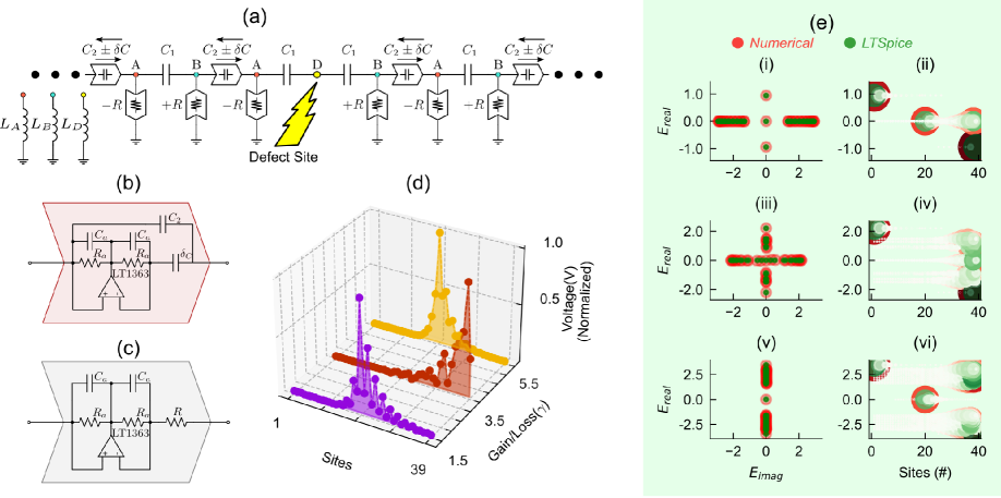
We designed an electrical circuit to realize the proposed model, and verify the interplay between non-Hermiticity, edge states, and topological defect states. Fig. 6(a) shows the circuit schematic with a total of nodes, including a defect site node in the middle. All other nodes are denoted as either or . Intra-cell coupling between nodes and is achieved with reciprocal capacitance , while inter-cell coupling is achieved with non-reciprocal capacitance . The non-reciprocal capacitance is realized using impedance converters at current inversion (INIC)[44, 71, 43, 38].
To drive the circuit at a frequency of kHz, nodes , , and are grounded through inductors , , and respectively, where , , and . To ensure consistency with our numerical results, we used nF, nF, nF, mH, mH, and mH. Additionally, to incorporate the on-site gain and loss term , we utilized positive and negative resistances () using INIC. To operate the circuit in PT, BPT, and APT regimes at the resonant frequency of 100 kHz, we used , , and respectively. Figs. 6(b) and (c) show the circuit schematic for non-reciprocal capacitance and using INIC. We chose and pF after analyzing the stability of the Operational Amplifier operating at kHz.
Fig. 6(d) shows the normalized node voltage profile when the circuit nodes were excited with current sources. For the PT symmetric case (, ), high voltage accumulation at the defect nodes confirms the theoretical predictions in 4(d). When the circuit operates in the Broken PT symmetric regime (, ), the defect node voltages disappear, appearing only at the right edges due to the presence of NHSE. However, under the APT symmetry (, ), the defect voltage accumulation reappears despite the presence of NHSE.
Fig. 6(e) shows the admittance eigenvalue spectrum and eigenstates reconstructed from the LTSpice simulations, compared with numerically calculated results. Red circles represent the numerical results, and green circles denote results from LTSpice simulations. By applying Kirchhoff’s current law, the circuit system response can be described by , where is the admittance matrix or circuit Laplacian, is the circuit Green’s function, and the vector components of and correspond to the input currents and voltages at the nodes. For an alternating current with angular frequency , the circuit Laplacian under periodic boundary conditions can be related to the lattice Hamiltonian by the relation, . To reconstruct the circuit Laplacian, we injected current to each node separately and measured all node voltages. These node voltages represent the first column of the circuit Green’s function, with being the circuit Laplacian.
For example, Fig. 6(e) (i)-(ii) shows the comparison for the circuit operating in the PT symmetric regime. Fig. 6(e)(i) shows that the theoretical admittance eigenspectrum (red) matches well with the energy values obtained from the LTSpice simulations (green). The eigenstates from the circuit Laplacian also match well with the theoretical results. In Fig. 6(e)(ii), higher accumulation at the defect node (Node ) with zero admittance energy is observed, while other states with zero admittance accumulate along the right edge. Additionally, there is edge state accumulation with admittance value of (normalized unit of ). Fig. 6(e)(iv) shows the results for the Broken PT symmetric case, where eigenstate accumulation at the defect node is no longer observed. However, in the APT case, the defect state reappears. These results confirm the practical implementation of the proposed defect model via a topolectrical circuit. As electrical circuits are versatile in design and operation, this implementation can be useful for practical applications.
V Conclusion
In conclusion, we have explored the interplay between NHSE and gain/loss terms with the topological edge and defect states in a finite SSH chain. As is well-known, the SSH chain hosts topological edge states localized at both ends of the chain. In the presence of conventional NHSE induced by non-reciprocity, both the topological edge states as well as bulk states are dragged towards a single preferred edge. However, with the introduction of staggered gain and loss terms to the sublattice sites, the topological edge states recover their original localization at both edges, while the bulk states retain their localization at the preferred edge. We also introduced defect sites in the chain and analyzed the properties of the resulting defect states under the influence of the NHSE and the underlying PT symmetry of the system. Interestingly, we found that the NHSE as well as the PT symmetry can modulate the localization of the defect state to occur either at the defect site or at the edges of the SSH chain, or to suppress the localization of the defect state completely. This is in contrast to the Stegmaier et al. (Ref. 68), which focused primarily on the activation / deactivation of defect states through gain / loss engineering. We also provided the analytical basis of this phenomenon of NHSE-controlled localization of defect states by evaluating the spatial profile of the eigenstates. Moreover, we proposed an experimental realization of our model using a TE circuit constructed from basic components such as capacitors, inductors, resistors and operational amplifiers. This circuit design validates our theoretical predictions by demonstrating the presence and control of defect states through its electrical characteristics, including voltage and admittance responses, modulated by non-Hermitian parameters. The ability to switch topological defect states and adjust their localization has significant implications for defect engineering in non-Hermitian systems. Our study provides new insights into the interplay between non-hermiticity and topological defect states, for the design and engineering of non-Hermitian systems with controllable and switchable defect states.
Acknowledgments
This work is supported by the Ministry of Education (MOE) of Singapore Tier-II Grant MOE-T2EP50121-0014 (NUS Grant No. A-8000086-01-00), and MOE Tier-I FRC Grant (NUS Grant No. A-8000195-01-00).
References
- Leykam et al. [2017] D. Leykam, K. Y. Bliokh, C. Huang, Y. D. Chong, and F. Nori, Edge modes, degeneracies, and topological numbers in non-hermitian systems, Phy. Rev. Lett. 118, 040401 (2017).
- Rafi-Ul-Islam et al. [2024a] S. Rafi-Ul-Islam, Z. B. Siu, M. S. H. Razo, and M. Jalil, Saturation dynamics in non-hermitian topological sensing systems, ArXiv preprint arXiv:2406.19629 (2024a).
- Ashida et al. [2020] Y. Ashida, Z. Gong, and M. Ueda, Non-hermitian physics, Adv. Phys. 69, 249 (2020).
- Siu et al. [2023] Z. B. Siu, S. Rafi-Ul-Islam, and M. B. Jalil, Terminal-coupling induced critical eigenspectrum transition in closed non-hermitian loops, Sci. Rep. 13, 22770 (2023).
- Rafi-Ul-Islam et al. [2024b] S. Rafi-Ul-Islam, Z. B. Siu, M. S. H. Razo, and M. Jalil, Exceptional points and braiding topology in non-hermitian systems with long-range coupling, ArXiv preprint arXiv:2407.04691 (2024b).
- Bergholtz et al. [2021] E. J. Bergholtz, J. C. Budich, and F. K. Kunst, Exceptional topology of non-hermitian systems, Rev. Mod. Phys. 93, 015005 (2021).
- Rafi-Ul-Islam et al. [2023a] S. Rafi-Ul-Islam, Z. B. Siu, H. Sahin, M. S. H. Razo, and M. Jalil, Twisted topology and bipolar non-hermitian skin effect induced by long-range asymmetric coupling, ArXiv preprint arXiv:2312.12780 (2023a).
- Gong et al. [2018] Z. Gong, Y. Ashida, K. Kawabata, K. Takasan, S. Higashikawa, and M. Ueda, Topological phases of non-hermitian systems, Phys. Rev. X 8, 031079 (2018).
- Yan et al. [2023] Q. Yan, B. Zhao, R. Zhou, R. Ma, Q. Lyu, S. Chu, X. Hu, and Q. Gong, Advances and applications on non-hermitian topological photonics, Nanophotonics (2023).
- Feng et al. [2017] L. Feng, R. El-Ganainy, and L. Ge, Non-hermitian photonics based on parity–time symmetry, Nat. Photon. 11, 752 (2017).
- Longhi [2018] S. Longhi, Parity-time symmetry meets photonics: A new twist in non-hermitian optics, Europhys. Lett. 120, 64001 (2018).
- Santra and Cederbaum [2002] R. Santra and L. S. Cederbaum, Non-hermitian electronic theory and applications to clusters, Phys. Rep. 368, 1 (2002).
- Wang et al. [2018] M. Wang, L. Ye, J. Christensen, and Z. Liu, Valley physics in non-hermitian artificial acoustic boron nitride, Phy. Rev. Lett. 120, 246601 (2018).
- Bagarello et al. [2016] F. Bagarello, R. Passante, and C. Trapani, Non-hermitian hamiltonians in quantum physics, Springer Proc. Phys. 184 (2016).
- Rafi-Ul-Islam et al. [2024c] S. Rafi-Ul-Islam, Z. B. Siu, M. S. H. Razo, H. Sahin, and M. B. Jalil, From knots to exceptional points: Emergence of topological features in non-hermitian systems with long-range coupling, Phys. Rev. B 110, 045444 (2024c).
- Zhang et al. [2019] D.-J. Zhang, Q.-h. Wang, and J. Gong, Time-dependent pt-symmetric quantum mechanics in generic non-hermitian systems, Phys. Rev. A 100, 062121 (2019).
- Longhi [2010] S. Longhi, Optical realization of relativistic non-hermitian quantum mechanics, Phy. Rev. Lett. 105, 013903 (2010).
- Bender et al. [2007] C. M. Bender, D. C. Brody, H. F. Jones, and B. K. Meister, Faster than hermitian quantum mechanics, Phy. Rev. Lett. 98, 040403 (2007).
- Ju et al. [2019] C.-Y. Ju, A. Miranowicz, G.-Y. Chen, and F. Nori, Non-hermitian hamiltonians and no-go theorems in quantum information, Phys. Rev. A 100, 062118 (2019).
- Hahn et al. [2016] C. Hahn, Y. Choi, J. W. Yoon, S. H. Song, C. H. Oh, and P. Berini, Observation of exceptional points in reconfigurable non-hermitian vector-field holographic lattices, Nat. Commun. 7, 12201 (2016).
- El-Ganainy et al. [2018] R. El-Ganainy, K. G. Makris, M. Khajavikhan, Z. H. Musslimani, S. Rotter, and D. N. Christodoulides, Non-hermitian physics and pt symmetry, Nat. Phys. 14, 11 (2018).
- Sahin et al. [2024] H. Sahin, H. Akgün, Z. B. Siu, S. Rafi-Ul-Islam, J. F. Kong, M. B. Jalil, and C. H. Lee, Protected chaos in a topological lattice, Adv. Sci. , e03216 (2024).
- Zhang et al. [2023] X. Zhang, B. Zhang, H. Sahin, Z. B. Siu, S. Rafi-Ul-Islam, J. F. Kong, B. Shen, M. B. Jalil, R. Thomale, and C. H. Lee, Anomalous fractal scaling in two-dimensional electric networks, Commun. Phys. 6, 151 (2023).
- Okuma et al. [2020] N. Okuma, K. Kawabata, K. Shiozaki, and M. Sato, Topological origin of non-hermitian skin effects, Phy. Rev. Lett. 124, 086801 (2020).
- Rafi-Ul-Islam et al. [2024d] S. M. Rafi-Ul-Islam, Z. B. Siu, H. Sahin, M. S. H. Razo, and M. B. A. Jalil, Twisted topology of non-hermitian systems induced by long-range coupling, Phys. Rev. B 109, 045410 (2024d).
- Rafi-Ul-Islam et al. [2024e] S. Rafi-Ul-Islam, Z. B. Siu, M. S. H. Razo, and M. Jalil, Dynamic manipulation of non-hermitian skin effect through frequency in topolectrical circuits, ArXiv preprint arXiv:2410.16914 (2024e).
- Rafi-Ul-Islam et al. [2025] S. Rafi-Ul-Islam, Z. B. Siu, M. S. H. Razo, and M. B. Jalil, Critical non-hermitian skin effect in a cross-coupled hermitian chain, Phys. Rev. B 111, 115415 (2025).
- Li et al. [2020] L. Li, C. H. Lee, S. Mu, and J. Gong, Critical non-hermitian skin effect, Nat. Commun. 11, 5491 (2020).
- Zhang et al. [2022] K. Zhang, Z. Yang, and C. Fang, Universal non-hermitian skin effect in two and higher dimensions, Nat. Commun. 13, 2496 (2022).
- Song et al. [2019] F. Song, S. Yao, and Z. Wang, Non-hermitian skin effect and chiral damping in open quantum systems, Phy. Rev. Lett. 123, 170401 (2019).
- Zhong et al. [2021] J. Zhong, K. Wang, Y. Park, V. Asadchy, C. C. Wojcik, A. Dutt, and S. Fan, Nontrivial point-gap topology and non-hermitian skin effect in photonic crystals, Phys. Rev. B 104, 125416 (2021).
- Zhu et al. [2020] X. Zhu, H. Wang, S. K. Gupta, H. Zhang, B. Xie, M. Lu, and Y. Chen, Photonic non-hermitian skin effect and non-bloch bulk-boundary correspondence, Phys. Rev. Res. 2, 013280 (2020).
- Song et al. [2020] Y. Song, W. Liu, L. Zheng, Y. Zhang, B. Wang, and P. Lu, Two-dimensional non-hermitian skin effect in a synthetic photonic lattice, Phys. Rev. Appl. 14, 064076 (2020).
- Rafi-Ul-Islam et al. [2020a] S. Rafi-Ul-Islam, Z. Bin Siu, and M. B. Jalil, Topoelectrical circuit realization of a weyl semimetal heterojunction, Commun. Phys. 3, 72 (2020a).
- Liu et al. [2021] S. Liu, R. Shao, S. Ma, L. Zhang, O. You, H. Wu, Y. J. Xiang, T. J. Cui, and S. Zhang, Non-hermitian skin effect in a non-hermitian electrical circuit, Research (2021).
- Rafi-Ul-Islam et al. [2020b] S. Rafi-Ul-Islam, Z. B. Siu, C. Sun, and M. B. Jalil, Realization of weyl semimetal phases in topoelectrical circuits, New J. Phys. 22, 023025 (2020b).
- Sahin et al. [2023] H. Sahin, Z. B. Siu, S. Rafi-Ul-Islam, J. F. Kong, M. B. Jalil, and C. H. Lee, Impedance responses and size-dependent resonances in topolectrical circuits via the method of images, Phys. Rev. B 107, 245114 (2023).
- Rafi-Ul-Islam et al. [2022a] S. Rafi-Ul-Islam, H. Sahin, Z. B. Siu, and M. B. Jalil, Interfacial skin modes at a non-hermitian heterojunction, Phys. Rev. Res. 4, 043021 (2022a).
- Helbig et al. [2020] T. Helbig, T. Hofmann, S. Imhof, M. Abdelghany, T. Kiessling, L. Molenkamp, C. Lee, A. Szameit, M. Greiter, and R. Thomale, Generalized bulk–boundary correspondence in non-hermitian topolectrical circuits, Nat. Phys. 16, 747 (2020).
- Rafi-Ul-Islam et al. [2023b] S. Rafi-Ul-Islam, Z. B. Siu, H. Sahin, and M. B. Jalil, Valley hall effect and kink states in topolectrical circuits, Phys. Rev. Res. 5, 013107 (2023b).
- Rafi-Ul-Islam et al. [2021a] S. Rafi-Ul-Islam, Z. B. Siu, and M. B. Jalil, Non-hermitian topological phases and exceptional lines in topolectrical circuits, New J. Phys. 23, 033014 (2021a).
- Hofmann et al. [2020] T. Hofmann, T. Helbig, F. Schindler, N. Salgo, M. Brzezińska, M. Greiter, T. Kiessling, D. Wolf, A. Vollhardt, A. Kabaši, et al., Reciprocal skin effect and its realization in a topolectrical circuit, Phys. Rev. Res. 2, 023265 (2020).
- Rafi-Ul-Islam et al. [2022b] S. Rafi-Ul-Islam, Z. B. Siu, H. Sahin, C. H. Lee, and M. B. Jalil, Unconventional skin modes in generalized topolectrical circuits with multiple asymmetric couplings, Phys. Rev. Res. 4, 043108 (2022b).
- Rafi-Ul-Islam et al. [2021b] S. Rafi-Ul-Islam, Z. B. Siu, and M. B. Jalil, Topological phases with higher winding numbers in nonreciprocal one-dimensional topolectrical circuits, Phys. Rev. B 103, 035420 (2021b).
- Xu et al. [2021] K. Xu, X. Zhang, K. Luo, R. Yu, D. Li, and H. Zhang, Coexistence of topological edge states and skin effects in the non-hermitian su-schrieffer-heeger model with long-range nonreciprocal hopping in topoelectric realizations, Phys. Rev. B 103, 125411 (2021).
- Zhang et al. [2021] X. Zhang, Y. Tian, J.-H. Jiang, M.-H. Lu, and Y.-F. Chen, Observation of higher-order non-hermitian skin effect, Nat. Commun. 12, 5377 (2021).
- Rafi-Ul-Islam et al. [2023c] S. Rafi-Ul-Islam, Z. B. Siu, H. Sahin, and M. B. Jalil, Conductance modulation and spin/valley polarized transmission in silicene coupled with ferroelectric layer, Journal of Magnetism and Magnetic Materials 571, 170559 (2023c).
- Kawabata et al. [2020] K. Kawabata, M. Sato, and K. Shiozaki, Higher-order non-hermitian skin effect, Phys. Rev. B 102, 205118 (2020).
- Rafi-Ul-Islam et al. [2023d] S. Rafi-Ul-Islam, Z. B. Siu, H. Sahin, and M. Jalil, Engineering higher-order dirac and weyl semimetallic phase in 3d topolectrical circuits, ArXiv preprint arXiv:2303.10911 (2023d).
- Lin et al. [2021] Z. Lin, S. Ke, X. Zhu, and X. Li, Square-root non-bloch topological insulators in non-hermitian ring resonators, Opt. Express 29, 8462 (2021).
- Rafi-Ul-Islam et al. [2024f] S. Rafi-Ul-Islam, Z. B. Siu, M. S. H. Razo, and M. Jalil, Anomalous non-hermitian skin effects in coupled hermitian chains with cross-coupling, ArXiv preprint arXiv:2410.21846 (2024f).
- Okuma and Sato [2021] N. Okuma and M. Sato, Quantum anomaly, non-hermitian skin effects, and entanglement entropy in open systems, Phys. Rev. B 103, 085428 (2021).
- Rafi-Ul-Islam et al. [2022c] S. Rafi-Ul-Islam, Z. B. Siu, H. Sahin, C. H. Lee, and M. B. Jalil, System size dependent topological zero modes in coupled topolectrical chains, Phys. Rev. B 106, 075158 (2022c).
- Fujita et al. [2011] T. Fujita, M. Jalil, S. Tan, and S. Murakami, Gauge fields in spintronics, J. Appl. Phys. 110 (2011).
- Rafi-Ul-Islam et al. [2024g] S. Rafi-Ul-Islam, Z. B. Siu, H. Sahin, and M. B. Jalil, Chiral surface and hinge states in higher-order weyl semimetallic circuits, Phys. Rev. B 109, 085430 (2024g).
- Obana et al. [2019] D. Obana, F. Liu, and K. Wakabayashi, Topological edge states in the su-schrieffer-heeger model, Phys. Rev. B 100, 075437 (2019).
- Hafezi et al. [2013] M. Hafezi, S. Mittal, J. Fan, A. Migdall, and J. Taylor, Imaging topological edge states in silicon photonics, Nat. Photon. 7, 1001 (2013).
- Rafi-Ul-Islam et al. [2022d] S. Rafi-Ul-Islam, Z. B. Siu, H. Sahin, and M. B. Jalil, Type-ii corner modes in topolectrical circuits, Phys. Rev. B 106, 245128 (2022d).
- Yuce [2018] C. Yuce, Edge states at the interface of non-hermitian systems, Phys. Rev. A 97, 042118 (2018).
- Esaki et al. [2011] K. Esaki, M. Sato, K. Hasebe, and M. Kohmoto, Edge states and topological phases in non-hermitian systems, Phys. Rev. B 84, 205128 (2011).
- Poli et al. [2015] C. Poli, M. Bellec, U. Kuhl, F. Mortessagne, and H. Schomerus, Selective enhancement of topologically induced interface states in a dielectric resonator chain, Na.Commun. 6, 6710 (2015).
- Blanco-Redondo et al. [2016] A. Blanco-Redondo, I. Andonegui, M. J. Collins, G. Harari, Y. Lumer, M. C. Rechtsman, B. J. Eggleton, and M. Segev, Topological optical waveguiding in silicon and the transition between topological and trivial defect states, Phys. Rev. Lett. 116, 163901 (2016).
- Lang et al. [2018] L.-J. Lang, Y. Wang, H. Wang, and Y. D. Chong, Effects of non-Hermiticity on Su-Schrieffer-Heeger defect states, Phys. Rev. B 98, 094307 (2018), publisher: American Physical Society.
- Cui et al. [2020] W.-X. Cui, L. Qi, Y. Xing, S. Liu, S. Zhang, and H.-F. Wang, Localized photonic states and dynamic process in nonreciprocal coupled su-schrieffer-heeger chain, Opt. Express 28, 37026 (2020).
- Kong et al. [2020] Z.-X. Kong, Y.-F. Zhang, H.-X. Hao, and W.-J. Gong, Energy spectra of coupled su-schrieffer-heeger chains with-symmetric imaginary boundary potentials, Phys. Scr. 95, 115801 (2020).
- Garmon and Noba [2021] S. Garmon and K. Noba, Reservoir-assisted symmetry breaking and coalesced zero-energy modes in an open pt-symmetric su-schrieffer-heeger model, Phys. Rev. A 104, 062215 (2021).
- Teo and Hughes [2017] J. C. Teo and T. L. Hughes, Topological defects in symmetry-protected topological phases, Annu. Rev. Condens. Matter Phys. 8, 211 (2017).
- Stegmaier et al. [2021] A. Stegmaier, S. Imhof, T. Helbig, T. Hofmann, C. H. Lee, M. Kremer, A. Fritzsche, T. Feichtner, S. Klembt, S. Höfling, et al., Topological defect engineering and p t symmetry in non-hermitian electrical circuits, Phys. Rev. Lett. 126, 215302 (2021).
- Barkeshli et al. [2013] M. Barkeshli, C.-M. Jian, and X.-L. Qi, Classification of topological defects in abelian topological states, Phys. Rev. B 88, 241103 (2013).
- Pan et al. [2018] M. Pan, H. Zhao, P. Miao, S. Longhi, and L. Feng, Photonic zero mode in a non-hermitian photonic lattice, Nat. Commun. 9, 1308 (2018).
- Rafi-Ul-Islam et al. [2022e] S. Rafi-Ul-Islam, Z. B. Siu, H. Sahin, C. H. Lee, and M. B. Jalil, Critical hybridization of skin modes in coupled non-hermitian chains, Phys. Rev. Res. 4, 013243 (2022e).
- Yao and Wang [2018] S. Yao and Z. Wang, Edge states and topological invariants of non-hermitian systems, Phys.Rev. Lett. 121, 086803 (2018).
- Munoz et al. [2018] F. Munoz, F. Pinilla, J. Mella, and M. I. Molina, Topological properties of a bipartite lattice of domain wall states, Sci. Rep. 8, 17330 (2018).
- Zurita et al. [2023] J. Zurita, C. E. Creffield, and G. Platero, Fast quantum transfer mediated by topological domain walls, Quantum 7, 1043 (2023).
- Marques and Dias [2022] A. Marques and R. Dias, Generalized lieb’s theorem for noninteracting non-hermitian n-partite tight-binding lattices, Phys. Rev. B 106, 205146 (2022).