A Roadmap for neutrino charge assignments in $U(2)_{F}$ Flavor Models: Implications for LFV processes and leptonic anomalous magnetic moments

Abstract

We build upon a simple $U(2)_{F}$ model of flavor, in which all fermion masses and mixing hierarchies arise from powers of two small parameters controlling $U(2)_{F}$ breaking. In the original formulation, an isomorphism to the discrete $D_{6}\times U(1)_{F}$ symmetry was invoked to generate a Majorana neutrino mass term. Here, we retain the successful features of that model for the charged leptons and quarks, while exploring alternative neutrino charge assignments within the $U(2)_{F}$ framework. This approach allows us to generate Majorana neutrino masses via the seesaw mechanism without introducing any additional symmetries nor invoking any isomorphism. We further examine the implications of our models for Lepton Flavor Violating (LFV) decays, analyzing the processes $\mu\rightarrow e\gamma$, $\tau\rightarrow\mu\gamma$ and $\tau\rightarrow e\gamma$ and their connection with the leptonic anomalous magnetic moments. We show that within the Standard Model Effective Field Theory (SMEFT) approach the current limits on the branching ratios of LFV decays obtained in our $U(2)_{F}$ models are not compatible with the anomaly observed for $(g-2)_{\mu}$, thereby suggesting that either $(g-2)_{\mu}$ must be very close to the Standard Model predictions or the invoked flavor symmetry is not appropriate to describe the current anomalies.

1 Introduction

In the last two decades, neutrino physics has undergone a strong revolution. The reason is related to the discovery of neutrino oscillations Super-Kamiokande:1998kpq , which are described by 6 real parameters: 2 mass squared differences $\Delta m_{\text{sol}}^{2}$ and $\Delta m_{\text{atm}}^{2}$, 3 mixing angles $\theta_{12}$, $\theta_{23}$ and $\theta_{13}$, and a CP violating phase $\delta_{\text{CP}}$. The presence of two mass squared differences implies that at least two of the three neutrino masses are nonzero, in contrast with the original formulation of the Standard Model (SM) where neutrinos were assumed massless Gaillard:1998ui .

Despite the increasingly precise knowledge of the oscillation parameters, several aspects of neutrino physics remain unknown. From the experimental point of view, current oscillation experiments could not be able to measure the absolute neutrino mass scale and present a limited capability of discerning a possible CP violation in the lepton sector as well as the neutrino mass ordering. From the theoretical point of view, there are no fully satisfactory theories which explain why neutrinos are massive and why their masses are so smaller compared to those of the other fermios. Moreover, the true nature of neutrinos, namely whether they are Dirac or Majorana particles Majorana:1937vz remains unknown. The neutrino mixing pattern makes also difficult to find a connection between quark and lepton properties; this is a part of the well-known flavor problem King:2003xn ; Feruglio:2015jfa ; Abbas:2023ivi . Indeed a different flavor mixing structure between quarks and leptons clearly emerges if we compare the entries of $V_{\text{CKM}}$ (the Cabibbo-Kobayashi-Maskawa matrix Cabibbo:1963yz ; Kobayashi:1973fv ) and $U_{\text{PMNS}}$ (the Pontecorvo-Maki-Nakagawa-Sakata matrix Pontecorvo:1957cp ; Pontecorvo:1957qd ; Maki:1962mu ; Pontecorvo:1967fh ): the former is almost diagonal, while the entries of the latter are almost all comparable to each other.

The search for an answer to all these questions and the need to give a flavor structure to the SM particles led to the proposal of various flavor symmetries, which constitute an extension to the SM gauge group $SU(3)_{C}\otimes SU(2)_{L}\otimes U(1)_{Y}$ and under which the three particle families transform in the same way. The general idea is the following: introduce one or more new scalar fields, which are neutral under the SM but charged under the chosen flavor symmetry. These fields, known as flavons, transform according to some irreducible representation of the flavor symmetry group. Flavons interact with leptons and the Higgs field according to the most general flavor-invariant Lagrangian, which is built considering all matter fields assigned to specific irreducible representations of the flavor group. The crucial point is that the flavons interact differently with various leptons, meaning the interactions are not universal. This non-uniform coupling allows for the construction of an invariant Lagrangian that, after flavor and gauge symmetry breaking, gives rise to the observed mixing matrix and mass spectrum.

Early oscillation data were well-compatible with a highly symmetric lepton mixing pattern, the Tri-Bi-Maximal (TB) one Harrison:2002er ; Harrison:2002kp ; Xing:2002sw ; Harrison:2002et ; Harrison:2003aw , which implies $\sin^{2}\theta_{12}=1/3$, $\sin^{2}\theta_{23}=1/2$ and $\theta_{13}=0$ and could be realized by non-abelian discrete symmetry (NADS) groups. Among the simplest groups we find $S_{3}$ Feruglio:2007hi , $A_{4}$ Altarelli:2005yp , and $S_{4}$ Bazzocchi:2009pv . However, since the discovery that the reactor mixing angle $\theta_{13}$ is nonzero DayaBay:2012fng , this approach has gradually lost interest, as these models require (large) deviations from the leading-order predictions in order to be successful Giarnetti:2024vgs — deviations that, we emphasize, can be nonetheless obtained from next-to-leading order corrections or by taking into account corrections from the charged lepton sector.

Recently Feruglio:2017spp , the NADS has regained popularity due to intriguing work on modular symmetries. These have been extensively studied within the context of string theory Feruglio:2019ybq . Interestingly, Feruglio demonstrated that it is always possible to find an isomorphism from the modular finite group $\Gamma_{N}$ of level $N\in\mathbb{N}$ to a non-abelian discrete symmetry group. In particular, for $N\leq 5$ the modular finite groups are isomorphic to $S_{3},A_{4},S_{4}$ and $A_{5}$. These models have attracted considerable attention, among other reasons, because they involve few free parameters, they do not generally require the presence of scalar fields like the flavons and are, therefore, more minimal and predictive. A list of few examples of such models follows: $\Gamma_{2}\cong S_{3}$ Kobayashi:2018vbk ; Marciano:2024nwm , $\Gamma_{3}\cong A_{4}$ Kobayashi:2018wkl ; Criado:2018thu ; Kobayashi:2018scp ; Okada:2018yrn ; Okada:2019uoy ; Ding:2019zxk ; Asaka:2019vev ; Okada:2021qdf ; Nomura:2022mgf ; Devi:2023vpe , $\Gamma_{4}\cong S_{4}$ Ding:2019gof ; Penedo:2018nmg ; Novichkov:2018ovf ; deMedeirosVarzielas:2019cyj and $\Gamma_{5}\cong A_{5}$ Criado:2019tzk ; Novichkov:2018nkm ; Ding:2019xna . Besides the NADS, alternative possibilities for addressing the neutrino mass and mixing problem based on continuous symmetries can be explored. The most minimal formulation relies on the addition of an abelian $U(1)_{F}$ symmetry group Leurer:1992wg ; Leurer:1993gy ; Dreiner:2003hw ; Petcov:1982ya ; Arcadi:2022ojj , whose main critical issue is its limited predictivity due to the large number of free parameters. For this reason, one can consider more predictive, though less minimal, models — such as those based on a $U(2)_{F}$ flavor symmetry Linster:2018avp ; Falkowski:2015zwa ; Barbieri:1995uv ; Barbieri:1997tu ; Dudas:2013pja . The original interest on these models was certainly related to their ability to explain the values of quark masses and mixing Barbieri:1995uv ; Barbieri:1997tu . But it has been also shown that, once extended to the neutrino sector, the $U(2)_{F}$ symmetry is able to adjust the values of the lepton mixing parameters. In addition, the New Physics (NP) interactions can induce Lepton Flavor Violating (LFV) decays and new contributions to the muon magnetic moment $(g-2)_{\mu}$ that, nowadays, has resumed a lot of interests because of the apparent disagreement among the latest measurements and the SM prediction Muong-2:2023cdq ; Muong-2:2021ojo ; Muong-2:2006rrc . This raises the interesting question of whether the same NP that explains neutrino masses and mixing could also mediate LFV processes — and under what constraints — and whether it might also be responsible for the anomalous magnetic moment of the muon. Numerous studies in the literature have explored this direction. For example, the electron and muon magnetic moments have been thoroughly analyzed within the framework of the Standard Model Effective Field Theory (SMEFT) Buchmuller:1985jz ; Grzadkowski:2010es ; Alonso:2013hga , where the new physics is assumed to lie above the Electroweak (EW) scale Panico:2018hal ; Aebischer:2021uvt ; Allwicher:2021rtd ; Kley:2021yhn . Other works investigate the connection between the muon’s anomalous magnetic moment $(g-2)_{\mu}$ and LFV processes, including scenarios involving modular flavor symmetries Kobayashi:2021pav ; Kobayashi:2022jvy , $U(2)_{L_{L}}\otimes U(2)_{E_{R}}$ flavor model Tanimoto:2023hse , and extended scalar sectors Chowdhury:2015sla ; DeJesus:2020yqx ; Esch:2016jyx ; Giarnetti:2023dcr ; Giarnetti:2024psj .

Driven by these motivations, we study a non-supersymmetric $U(2)_{F}$ model of flavor, which is inspired by the analyses performed in Linster:2018avp where the proposed model has been shown to reproduce the quarks and leptons observables. However, differently from Linster:2018avp where a $D_{6}\times U(1)_{F}$ flavor symmetry is introduced for getting Majorana neutrino masses from the Weinberg operator, we provide see-saw neutrino Majorana mass terms solely within $U(2)_{F}$ by relaxing the charge requirements and making use of the arbitrariness in the assignment of the $U(2)_{F}$ quantum numbers to the right-handed (RH) neutrinos.

The paper is organized as follows: in Sec. 2, we describe the relevant features of our constructions. In Sec. 3 we provide a catalog of possible neutrino mass matrices, obtained via the type-I see-saw mechanism. Subsequently we derive predictions on the physical observables $m_{\beta}$ and $m_{\beta\beta}$. In Sec. 4, we analyse the LFV decays in light of the $(g-2)_{\mu}$ anomalous magnetic moment and we discuss our results in the Conclusions, Sec. 5.

2 A realistic $U(2)_{F}$ model of flavor

The first $U(2)_{F}$ models have been proposed in Barbieri:1995uv ; Barbieri:1997tu in the context of SUSY, with flavor quantum numbers compatible with a unified SO(10) gauge group. In that case, the special structure of quark mass matrices lead to the prediction $V_{ub}/V_{cb}=m_{u}/m_{c}$ (with $V\equiv V_{CKM}$), which is strongly disfavored by the data. However, it was shown that a viable $U(2)_{F}$ model with flavor quantum numbers compatible only with an unified $SU(5)$ gauge group was possible Dudas:2013pja ; Falkowski:2015zwa . This class of models does not require the presence of SUSY.

In this paper we will follow the latter approach; the breaking of the $U(2)_{F}$ flavor symmetry is described by two flavons $\phi$ and $\chi$, whose VEVs determine the hierarchical structure of the mass matrices in the various fermionic sectors of the SM.

2.1 The charged lepton sector

We work with a global $U(2)_{F}$ symmetry, which is broken slightly below a cutoff scale $\Lambda$, corresponding to the mass scale of the new degrees of freedom. This mass scale must be very high to ensure that such additional dynamics do not affect the low-energy phenomenology we are interested in. It can be demonstrated that $U(2)_{F}$ is locally isomorphic to $SU(2)_{F}\times U(1)_{F}$. Here we briefly revise the sucessfull construction described in Linster:2018avp , whose field quantum numbers are the good ones to reproduce the quarks masses and CKM mixing as well as the ratio of the charged lepton masses, see Table 1, Linster:2018avp ; Falkowski:2015zwa .

Fields / Representations	$\mathbf{SU(2)_{F}}$	$\mathbf{U(1)_{F}}$
$L_{a}$ ,  $D_{a}$ ,  $Q_{a}$ ,  $U_{a}$ ,  $E_{a}$    ($a=1,2$)	$2$	+$1$
$Q_{3}$ ,  $U_{3}$ ,  $E_{3}$	$1$	+$0$
$L_{3}$ ,  $D_{3}$	$1$	+$1$
$\phi_{a}$    ($a=1,2$)	$2$	$-1$
$\chi$	$1$	$-1$

Table 1: $SU(2)_{F}$ and $U(1)_{F}$ quantum numbers of SM fermions and flavons. The SM fermions are organized into representations of the Standard Model gauge group. The Higgs is a singlet under both $SU(2)_{F}$ and $U(1)_{F}$.

Here, $L$ and $Q$ contain the SM left-handed lepton doublet and quark doublet, respectively, while $E$, $D$ and $U$ are the SM right-handed electron, down quark and up quark. Each representation has three generations corresponding to the three flavors. As we can see from Table 1, the first two generations transform as $SU(2)_{F}$ doublets and the third generations as singlets. It is worth specifying that $SU(2)_{F}$ doublets and singlets should not be confused with the $SU(2)_{L}$ isospin doublets and singlets of the SM. Regarding the scalar fields, the Higgs ($H$) is a singlet under both $SU(2)_{F}$ and $U(1)_{F}$, while the flavons $\phi$ and $\chi$ are an $SU(2)_{F}$ doublet and singlet, respectively. This charge assignments are compatible with an $SU(5)$ GUT structure Georgi:1974sy , on which we will not further elaborate in this paper.

Since fermions are charged under $U(2)_{F}$, constructing invariant terms in the Lagrangian necessitates additional flavon insertions. This leads to the following form of the charged lepton Lagrangian:

$$\begin{split}\mathcal{L}_{e}&=\frac{e_{11}}{\Lambda^{6}}\chi^{4}(\widetilde{\phi}L)_{1}(\widetilde{\phi}E)_{1}H+\frac{e_{12}}{\Lambda^{2}}\chi^{2}(LE)_{1}H+\frac{e_{13}}{\Lambda^{3}}\chi^{2}(\widetilde{\phi}L)_{1}E_{3}H\ +\\ &+\frac{e_{22}}{\Lambda^{2}}(\phi L)_{1}(\phi E)_{1}H+\frac{e_{23}}{\Lambda}(\phi L)_{1}E_{3}H+\frac{e_{31}}{\Lambda^{4}}\chi^{3}L_{3}(\widetilde{\phi}E)_{1}H\ +\\ &+\frac{e_{32}}{\Lambda^{2}}\chi L_{3}(\phi E)_{1}H+\frac{e_{33}}{\Lambda}\chi L_{3}E_{3}H\ ,\end{split}$$ (1)

where $\widetilde{\phi}=i\sigma_{2}\phi^{*}$. With the notation $(AB)_{1}$ we refer to the contraction of the fields $A$ and $B$ into an $SU(2)_{F}$ singlet.

The two flavon fields acquire the following vacuum expectation values (VEVs):

$$\langle\phi\rangle=\begin{pmatrix}\varepsilon_{\phi}\Lambda\\ 0\\ \end{pmatrix}\hskip 36.98866pt\text{and}\hskip 36.98866pt\langle\chi\rangle=\varepsilon_{\chi}\Lambda\ ,$$ (2)

where we assume that $\varepsilon_{\phi,\chi}\ll 1$ (and they will be used as our expansion parameters) and $\Lambda$ is the cut-off scale of the effective theory. These flavon VEVs determine the presence of the powers of $\varepsilon_{\phi}$ and $\varepsilon_{\chi}$ in the entries of the Yukawa matrices, which bring out the hierarchies.

It was shown in Refs. Linster:2018avp ; Falkowski:2015zwa that the quark and charged lepton mass ratios, along with the CKM matrix elements, can be accommodated within their $1\sigma$ experimental ranges at a scale of 10 TeV by taking

$$\varepsilon_{\phi}\sim\lambda^{2}\hskip 42.67912pt\text{and}\hskip 42.67912pt\varepsilon_{\chi}\sim\lambda^{2\text{\textdiv}3}\ ,$$ (3)

where $\lambda=0.2$ is roughly the Wolfenstein parameter Liu:2014gla , which correspond, to a first approximation, to the sine of the Cabibbo angle Roy:2014nua .

Since we are going to use it later on this paper, it is worth showing the Yukawa matrix of the charged lepton sector, obtained from the Lagrangian of eq. (1):

$$Y_{e}\approx\begin{pmatrix}e_{11}\varepsilon_{\phi}^{2}\varepsilon_{\chi}^{4}&e_{12}\varepsilon_{\chi}^{2}&e_{13}\varepsilon_{\phi}\varepsilon_{\chi}^{2}\\ -e_{12}\varepsilon_{\chi}^{2}&e_{22}\varepsilon_{\phi}^{2}&e_{23}\varepsilon_{\phi}\\ e_{31}\varepsilon_{\phi}\varepsilon_{\chi}^{3}&e_{32}\varepsilon_{\phi}\varepsilon_{\chi}&e_{33}\varepsilon_{\chi}\\ \end{pmatrix}\ ,$$ (4)

where $e_{ij}$ are (in general) complex $\mathcal{O}(1)$ coefficients.

3 The neutrino sector revised

In this Section, we will assume both the existence of the right-handed (RH) neutrinos and Lepton Number Violation (LNV) interactions. The three generations of RH neutrinos $N_{i}$ transform as singlets under the Standard Model gauge group and, in general, as a given representation $N$ under the flavor symmetry group. In Linster:2018avp , an attempt to apply the $U(2)_{F}$ to neutrinos was already done. However, they restricted the analysis only on positive (or null) $U(1)_{F}$ charges and considered only the possibility in which the first two generations of $N$ transform as an $SU(2)_{F}$ doublet, while the third as a singlet. This latter assumption, which seems to be the most natural (it follows that of left-handed neutrinos, see Table 1), lead to predictions that are incompatible with the physical data. In addition to the previous attempts, we consider here all other possible $SU(2)_{F}$ and $U(1)_{F}$ quantum numbers for $N_{1}$, $N_{2}$ and $N_{3}$, on which we impose no constraints related to their signs. As we will see, this arbitrariness leads to a large number of neutrino mass matrix structures, which we will call patterns. Each mass matrix pattern will be analyzed in order to see whether they are able to reproduce neutrino masses and mixing.

3.1 Catalog of possible mass matrices

The three generations of the right-handed neutrinos can transform under $SU(2)_{F}$ in three different ways, which correspond to three different Models, as follows:

• Model S: $N_{1}$, $N_{2}$ and $N_{3}$ transform as 3 independent $SU(2)_{F}$ singlets;

• Model D: $N_{a}$ ($a=1,2$) transform as a doublet of $SU(2)_{F}$, while $N_{3}$ as a singlet;

• Model T: $N_{i}$ ($i=1,2,3$) transform as a triplet of $SU(2)_{F}$.

A graphical representation of the three Models is reported in Fig. 1.

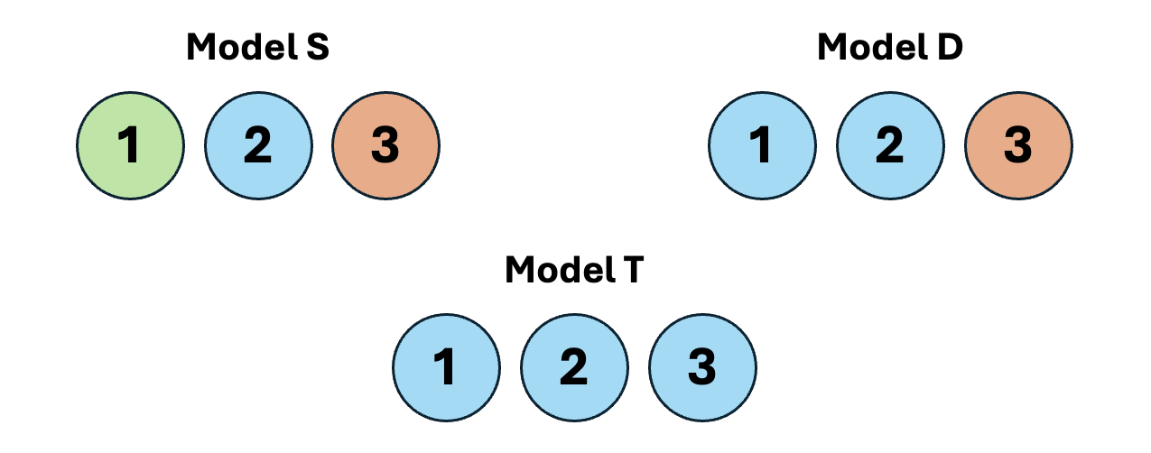
Figure 1: Graphic representation of the three Models that come out in the $SU(2)_{F}$ application to Majorana neutrinos. The numbers $1,2,3$ correspond to $N_{1},N_{2},N_{3}$. Different colours correspond to different $SU(2)_{F}$ representations (for example, Model D has the blue corresponding to the doublet and the red corresponding to the singlet).

Notice that in Model D one should consider three different sub-cases, corresponding to the three different dispositions of the singlet (it can be $N_{1}$, $N_{2}$ or $N_{3}$). However, it can be demonstrated that these three cases are equivalent and give the same results, so we will consider only the case in which $N_{3}$ is the singlet, as quoted above.

The Yukawa couplings and the Majorana mass term reads:

$$\mathcal{L}_{\nu}=L^{T}Y_{\nu}NH+\frac{1}{2}N^{T}M_{\nu}N+h.c.\ ,$$ (5)

where $Y_{\nu}$ is the Yukawa matrix, $M_{\nu}$ is the Majorana mass matrix. In the Model S, all the three generations of $N$ are $SU(2)_{F}$ singlets, so their $U(1)_{F}$ charges will be indicated as three different variables $X_{1}$, $X_{2}$ and $X_{3}$. The $U(2)_{F}$ invariant Yukawa coupling terms for the Model S are:

$$\begin{split}\mathcal{L}_{\nu}^{yuk(S)}&=\frac{y_{11}}{\Lambda^{1+\lvert 2+X_{1}\rvert}}\chi^{\lvert 2+X_{1}\rvert}(\widetilde{\phi}L)_{1}N_{1}H+\frac{y_{12}}{\Lambda^{1+\lvert 2+X_{2}\rvert}}\chi^{\lvert 2+X_{2}\rvert}(\widetilde{\phi}L)_{1}N_{2}H\\ &+\frac{y_{13}}{\Lambda^{1+\lvert 2+X_{3}\rvert}}\chi^{\lvert 2+X_{3}\rvert}(\widetilde{\phi}L)_{1}N_{3}H+\frac{y_{21}}{\Lambda^{1+\lvert X_{1}\rvert}}\chi^{\lvert X_{1}\rvert}(\phi L)_{1}N_{1}H\\ &+\frac{y_{22}}{\Lambda^{1+\lvert X_{2}\rvert}}\chi^{\lvert X_{2}\rvert}(\phi L)_{1}N_{2}H+\frac{y_{23}}{\Lambda^{1+\lvert X_{3}\rvert}}\chi^{\lvert X_{3}\rvert}(\phi L)_{1}N_{3}H\\ &+\frac{y_{31}}{\Lambda^{\lvert 1+X_{1}\rvert}}\chi^{\lvert 1+X_{1}\rvert}L_{3}N_{1}H+\frac{y_{32}}{\Lambda^{\lvert 1+X_{2}\rvert}}\chi^{\lvert 1+X_{2}\rvert}L_{3}N_{2}H\\ &+\frac{y_{33}}{\Lambda^{\lvert 1+X_{3}\rvert}}\chi^{\lvert 1+X_{3}\rvert}L_{3}N_{3}H\ .\end{split}$$ (6)

For each possible coupling of the Lagrangian, we have shown the leading order (LO) term only, i.e. the one with the least number of flavon fields. $y_{ij}$ are $\mathcal{O}(1)$ complex coefficients. For the Majorana mass term we have instead:

$$\begin{split}\mathcal{L}_{\nu}^{M(S)}&=\frac{k_{11}}{\Lambda^{\lvert 2X_{1}\rvert}}\chi^{\lvert 2X_{1}\rvert}N_{1}N_{1}+\frac{k_{12}}{\Lambda^{\lvert X_{1}+X_{2}\rvert}}\chi^{\lvert X_{1}+X_{2}\rvert}N_{1}N_{2}\\ &+\frac{k_{13}}{\Lambda^{\lvert X_{1}+X_{3}\rvert}}\chi^{\lvert X_{1}+X_{3}\rvert}N_{1}N_{3}+\frac{k_{22}}{\Lambda^{\lvert 2X_{2}\rvert}}\chi^{\lvert 2X_{2}\rvert}N_{2}N_{2}\\ &+\frac{k_{23}}{\Lambda^{\lvert X_{2}+X_{3}\rvert}}\chi^{\lvert X_{2}+X_{3}\rvert}N_{2}N_{3}+\frac{k_{33}}{\Lambda^{\lvert 2X_{3}\rvert}}\chi^{\lvert 2X_{3}\rvert}N_{3}N_{3}\ ,\end{split}$$ (7)

where $k_{ij}$ are $\mathcal{O}(1)$ complex coefficients.

After inserting the flavon VEVs of eq. (2), the dependence on $\Lambda$ disappears and, writing the Lagrangian in the compact form of eq. (5), we derive the following Yukawa matrix and Majorana mass matrix:

$$Y_{\nu}^{S}=\begin{pmatrix}y_{11}\varepsilon_{\phi}\varepsilon_{\chi}^{\lvert 2+X_{1}\rvert}&y_{12}\varepsilon_{\phi}\varepsilon_{\chi}^{\lvert 2+X_{2}\rvert}&y_{13}\varepsilon_{\phi}\varepsilon_{\chi}^{\lvert 2+X_{3}\rvert}\\ y_{21}\varepsilon_{\phi}\varepsilon_{\chi}^{\lvert X_{1}\rvert}&y_{22}\varepsilon_{\phi}\varepsilon_{\chi}^{\lvert X_{2}\rvert}&y_{23}\varepsilon_{\phi}\varepsilon_{\chi}^{\lvert X_{3}\rvert}\\ y_{31}\varepsilon_{\chi}^{\lvert 1+X_{1}\rvert}&y_{32}\varepsilon_{\chi}^{\lvert 1+X_{2}\rvert}&y_{33}\varepsilon_{\chi}^{\lvert 1+X_{3}\rvert}\\ \end{pmatrix}$$ (8)

and

$$M_{\nu}^{S}=M\begin{pmatrix}k_{11}\varepsilon_{\chi}^{\lvert 2X_{1}\rvert}&k_{12}\varepsilon_{\chi}^{\lvert X_{1}+X_{2}\rvert}&k_{13}\varepsilon_{\chi}^{\lvert X_{1}+X_{3}\rvert}\\ k_{12}\varepsilon_{\chi}^{\lvert X_{1}+X_{2}\rvert}&k_{22}\varepsilon_{\chi}^{\lvert 2X_{2}\rvert}&k_{23}\varepsilon_{\chi}^{\lvert X_{2}+X_{3}\rvert}\\ k_{13}\varepsilon_{\chi}^{\lvert X_{1}+X_{3}\rvert}&k_{23}\varepsilon_{\chi}^{\lvert X_{2}+X_{3}\rvert}&k_{33}\varepsilon_{\chi}^{\lvert 2X_{3}\rvert}\\ \end{pmatrix}\ ,$$ (9)

where $M$ is the mass scale of the RH neutrinos, which we expect to be of order $10^{14}~\text{GeV}$, as in the usual see-saw. It is worth noting that the model is not supersymmetric, so whenever an exponent in the two matrices becomes negative, we can still replace the scalar field $\chi$ with its conjugated to ensure that only positive powers in the expansion parameter $\varepsilon_{\chi}$ appear.

The light neutrino mass matrix $m_{\nu}^{M}$ is obtained via the type-I see-saw mechanism Brdar:2019iem , according to the master formula:

$$m_{\nu}^{M}=-v^{2}\ Y_{\nu}M_{\nu}^{-1}Y_{\nu}^{T}\ .$$ (10)

As this expression holds for all three models, we omit the superscripts from $Y_{\nu}$ and $M_{\nu}$ to simplify the notation.

The choice of charges for the right-handed neutrinos leads to differences in the parametric structure of the neutrino mass matrix because of the moduli in (8) and (9), which act as a sign change on the arguments of the exponentials when they become negative. For example, for $X_{1},X_{2},X_{3}\geq 0$ all the quantities within the moduli in $Y_{\nu}^{S}$ and $M_{\nu}^{S}$ are $\geq 0$, for $(X_{1},X_{2},X_{3})=(-1,0,0)$ some are negative and for $X_{1},X_{2},X_{3}\leq-2$ they are all negative. For each case we will have a different resulting matrix. Thus, for the same Model, we get a finite number of different mass matrices, that we call patterns. We will discuss more about that in the following.

In Model D, the $U(1)_{F}$ charges are $X_{D}$ and $X_{3}$, associated with the $N_{a}$ ($a=1,2$) doublet and $N_{3}$, respectively. The two terms of the Lagrangian are in this case:

$$\begin{split}\mathcal{L}_{\nu}^{yuk(D)}&=\frac{y_{11}}{\Lambda^{2+\lvert 3+X_{D}\rvert}}\chi^{\lvert 3+X_{D}\rvert}(\widetilde{\phi}L)_{1}(\widetilde{\phi}N)_{1}H+\frac{y_{12}}{\Lambda^{\lvert 1+X_{D}\rvert}}\chi^{\lvert 1+X_{D}\rvert}(LN)_{1}H\\ &+\frac{y_{13}}{\Lambda^{1+\lvert 2+X_{3}\rvert}}\chi^{\lvert 2+X_{3}\rvert}(\widetilde{\phi}L)_{1}N_{3}H+\frac{y_{22}}{\Lambda^{2+\lvert X_{D}-1\rvert}}\chi^{\lvert X_{D}-1\rvert}(\phi L)_{1}(\phi N)_{1}H\\ &+\frac{y_{23}}{\Lambda^{1+\lvert X_{3}\rvert}}\chi^{\lvert X_{3}\rvert}(\phi L)_{1}N_{3}H+\frac{y_{31}}{\Lambda^{1+\lvert 2+X_{D}\rvert}}\chi^{\lvert 2+X_{D}\rvert}L_{3}(\widetilde{\phi}N)_{1}H\\ &+\frac{y_{32}}{\Lambda^{1+\lvert X_{D}\rvert}}\chi^{\lvert X_{D}\rvert}L_{3}(\phi N)_{1}H+\frac{y_{33}}{\Lambda^{\lvert 1+X_{3}\rvert}}\chi^{\lvert 1+X_{3}\rvert}L_{3}N_{3}H\end{split}$$ (11)

and

$$\begin{split}\mathcal{L}_{\nu}^{M(D)}&=\frac{k_{11}}{\Lambda^{2+\lvert 2+2X_{D}\rvert}}\chi^{\lvert 2+2X_{D}\rvert}(\widetilde{\phi}N)_{1}(\widetilde{\phi}N)_{1}+\frac{k_{12}}{\Lambda^{2+\lvert 2X_{D}\rvert}}\chi^{\lvert 2X_{D}\rvert}(\widetilde{\phi}N)_{1}(\phi N)_{1}\\ &+\frac{k_{13}}{\Lambda^{1+\lvert 1+X_{D}+X_{3}\rvert}}\chi^{\lvert 1+X_{D}+X_{3}\rvert}(\widetilde{\phi}N)_{1}N_{3}\\ &+\frac{k_{22}}{\Lambda^{2+\lvert 2X_{D}-2\rvert}}\chi^{\lvert 2X_{D}-2\rvert}(\phi N)_{1}(\phi N)_{1}\\ &+\frac{k_{23}}{\Lambda^{1+\lvert X_{D}+X_{3}-1\rvert}}\chi^{\lvert X_{D}+X_{3}-1\rvert}(\phi N)_{1}N_{3}+\frac{k_{33}}{\Lambda^{\lvert 2X_{3}\rvert}}\chi^{\lvert 2X_{3}\rvert}N_{3}N_{3}\ .\end{split}$$ (12)

Inserting the flavon VEVs in eqs. (11) and (12), we obtain

$$Y_{\nu}^{D}\approx\begin{pmatrix}y_{11}\varepsilon_{\phi}^{2}\varepsilon_{\chi}^{\lvert 3+X_{D}\rvert}&y_{12}\varepsilon_{\chi}^{\lvert 1+X_{D}\rvert}&y_{13}\varepsilon_{\phi}\varepsilon_{\chi}^{\lvert 2+X_{3}\rvert}\\ -y_{12}\varepsilon_{\chi}^{\lvert 1+X_{D}\rvert}&y_{22}\varepsilon_{\phi}^{2}\varepsilon_{\chi}^{\lvert X_{D}-1\rvert}&y_{23}\varepsilon_{\phi}\varepsilon_{\chi}^{\lvert X_{3}\rvert}\\ y_{31}\varepsilon_{\phi}\varepsilon_{\chi}^{\lvert 2+X_{D}\rvert}&y_{32}\varepsilon_{\phi}\varepsilon_{\chi}^{\lvert X_{D}\rvert}&y_{33}\varepsilon_{\chi}^{\lvert 1+X_{3}\rvert}\\ \end{pmatrix}\,,$$ (13)

and

$$M_{\nu}^{D}=M\begin{pmatrix}k_{11}\varepsilon_{\phi}^{2}\varepsilon_{\chi}^{\lvert 2+2X_{D}\rvert}&k_{12}\varepsilon_{\phi}^{2}\varepsilon_{\chi}^{\lvert 2X_{D}\rvert}&k_{13}\varepsilon_{\phi}\varepsilon_{\chi}^{\lvert 1+X_{D}+X_{3}\rvert}\\ k_{12}\varepsilon_{\phi}^{2}\varepsilon_{\chi}^{\lvert 2X_{D}\rvert}&k_{22}\varepsilon_{\phi}^{2}\varepsilon_{\chi}^{\lvert 2X_{D}-2\rvert}&k_{23}\varepsilon_{\phi}\varepsilon_{\chi}^{\lvert X_{D}+X_{3}-1\rvert}\\ k_{13}\varepsilon_{\phi}\varepsilon_{\chi}^{\lvert 1+X_{D}+X_{3}\rvert}&k_{23}\varepsilon_{\phi}\varepsilon_{\chi}^{\lvert X_{D}+X_{3}-1\rvert}&k_{33}\varepsilon_{\chi}^{\lvert 2X_{3}\rvert}\\ \end{pmatrix}\,.$$ (14)

Note that in the (12) entry of the Majorana mass matrix, the term without $\epsilon_{\phi}^{2}$ (corresponding to $(NN)_{1}$) vanishes because of the antisymmetric nature of the $SU(2)_{F}$ singlet contraction. For this reason, a double insertion of the flavon $\phi$ is required. The light neutrino mass is given by eq. (10) and, also in this case, there are a finite number of different patterns.

Finally, for Model T, the three RH neutrinos transform as a triplet $N_{i}$ ($i=1,2,3$) under the $U(1)_{F}$ symmetry group, with charge $X_{T}$. The two $U(2)_{F}$ invariant terms of the Lagrangian are therefore

$$\begin{split}\mathcal{L}_{\nu}^{yuk(T)}&=\frac{y_{11}}{\Lambda^{3+\lvert 4+X_{T}\rvert}}\chi^{\lvert 4+X_{T}\rvert}(\widetilde{\phi}\widetilde{\phi}\widetilde{\phi}LN)_{1}H+\frac{y_{12}}{\Lambda^{1+\lvert 2+X_{T}\rvert}}\chi^{\lvert 2+X_{T}\rvert}(\widetilde{\phi}LN)_{1}H\\ &+\frac{y_{13}}{\Lambda^{1+\lvert X_{T}\rvert}}\chi^{\lvert X_{T}\rvert}(\phi LN)_{1}H+\frac{y_{23}}{\Lambda^{3+\lvert X_{T}-2\rvert}}\chi^{\lvert X_{T}-2\rvert}(\phi\phi\phi LN)_{1}H\\ &+\frac{y_{31}}{\Lambda^{2+\lvert 3+X_{T}\rvert}}\chi^{\lvert 3+X_{T}\rvert}L_{3}(\widetilde{\phi}\widetilde{\phi}N)_{1}H+\frac{y_{32}}{\Lambda^{2+\lvert 1+X_{T}\rvert}}\chi^{\lvert 1+X_{T}\rvert}L_{3}(\phi\widetilde{\phi}N)_{1}H\\ &+\frac{y_{33}}{\Lambda^{2+\lvert X_{T}-1\rvert}}\chi^{\lvert X_{T}-1\rvert}L_{3}(\phi\phi N)_{1}H\end{split}$$ (15)

and

$$\begin{split}\mathcal{L}_{\nu}^{M(T)}&=\frac{k_{11}}{\Lambda^{4+\lvert 4+2X_{T}\rvert}}\chi^{\lvert 4+2X_{T}\rvert}(\widetilde{\phi}\widetilde{\phi}N\widetilde{\phi}\widetilde{\phi}N)_{1}+\frac{k_{12}}{\Lambda^{4+\lvert 2+2X_{T}\rvert}}\chi^{\lvert 2+2X_{T}\rvert}(\widetilde{\phi}\widetilde{\phi}N\widetilde{\phi}\phi N)_{1}\\ &+\frac{k_{13}}{\Lambda^{\lvert 2X_{T}\rvert}}\chi^{\lvert 2X_{T}\rvert}(NN)_{1}+\frac{k_{23}}{\Lambda^{4+\lvert 2X_{T}-2\rvert}}\chi^{\lvert 2X_{T}-2\rvert}(\phi\phi N\phi\widetilde{\phi}N)_{1}\\ &+\frac{k_{33}}{\Lambda^{4+\lvert 2X_{T}-4\rvert}}\chi^{\lvert 2X_{T}-4\rvert}(\phi\phi N\phi\phi N)_{1}\ ,\end{split}$$ (16)

where the subscript "1" indicates, as before, the singlet contraction of all fields within the parentheses.

If we insert the flavon VEVs in eqs. (15) and (16), we obtain

$$Y_{\nu}^{T}\approx\begin{pmatrix}y_{11}\varepsilon_{\phi}^{3}\varepsilon_{\chi}^{\lvert 4+X_{T}\rvert}&y_{12}\varepsilon_{\phi}\varepsilon_{\chi}^{\lvert 2+X_{T}\rvert}&\sqrt{2}y_{13}\varepsilon_{\phi}\varepsilon_{\chi}^{\lvert X_{T}\rvert}\\ -\sqrt{2}y_{12}\varepsilon_{\phi}\varepsilon_{\chi}^{\lvert 2+X_{T}\rvert}&-y_{13}\varepsilon_{\phi}\varepsilon_{\chi}^{\lvert X_{T}\rvert}&y_{23}\varepsilon_{\phi}^{3}\varepsilon_{\chi}^{\lvert X_{T}-2\rvert}\\ y_{31}\varepsilon_{\phi}^{2}\varepsilon_{\chi}^{\lvert 3+X_{T}\rvert}&y_{32}\varepsilon_{\phi}^{2}\varepsilon_{\chi}^{\lvert 1+X_{T}\rvert}&y_{33}\varepsilon_{\phi}^{2}\varepsilon_{\chi}^{\lvert X_{T}-1\rvert}\\ \end{pmatrix}$$ (17)

and

$$M_{\nu}^{T}=M\begin{pmatrix}k_{11}\varepsilon_{\phi}^{4}\varepsilon_{\chi}^{\lvert 4+2X_{T}\rvert}&k_{12}\varepsilon_{\phi}^{4}\varepsilon_{\chi}^{\lvert 2+2X_{T}\rvert}&k_{13}\varepsilon_{\chi}^{\lvert 2X_{T}\rvert}\\ k_{12}\varepsilon_{\phi}^{4}\varepsilon_{\chi}^{\lvert 2+2X_{T}\rvert}&-k_{13}\varepsilon_{\chi}^{\lvert 2X_{T}\rvert}&k_{23}\varepsilon_{\phi}^{4}\varepsilon_{\chi}^{\lvert 2X_{T}-2\rvert}\\ k_{13}\varepsilon_{\chi}^{\lvert 2X_{T}\rvert}&k_{23}\varepsilon_{\phi}^{4}\varepsilon_{\chi}^{\lvert 2X_{T}-2\rvert}&k_{33}\varepsilon_{\phi}^{4}\varepsilon_{\chi}^{\lvert 2X_{T}-4\rvert}\\ \end{pmatrix}\ ,$$ (18)

from which we get the light neutrino mass matrix with the various patterns.

3.1.1 Classification of the matrices

When we analyzed the reliability of the $U(2)_{F}$ model on quarks and charged leptons (see Section 2.1), we said that the fermion mass ratios and the CKM entries can be approximately reproduced following the parameterization of the VEVs given in eq. (3). Therefore, we consider the following two cases:

$$\varepsilon_{\phi}=\varepsilon_{\chi}=\lambda^{2}\ ,$$ (19)

$$\varepsilon_{\phi}=\lambda^{2}\hskip 17.07182pt\text{and}\hskip 17.07182pt\varepsilon_{\chi}=\lambda^{3}\ ,$$ (20)

so that all patterns are characterized by the powers of a single parameter $\lambda$. We refer to the A-Scenario as that corresponding to eq. (19) and to the B-Scenario as that of eq. (20).

We have therefore the following situation: there are three different Models (Model S, D and T) arising from the transformation properties of the three generations of $N$ under $SU(2)_{F}$. For each Model, there is a finite number of different patterns arising from different choices of the $U(1)_{F}$ charges for the three RH neutrinos $N_{i}$ and these patterns change depending on whether A-Scenario or B-Scenario is considered.

It is worth to notice that there are many cases in which different $U(1)_{F}$ charge assignments lead to the same mass matrix at LO. For example, if we consider Model D with A-Scenario, we have the same LO pattern for different charge assignments $(X_{D},X_{3})=\{(-2,-1),(-1,-1),(-2,-2)\}$. We have chosen to identify as equal two different mass matrices if they differ by terms that are at least a factor $\lambda^{4}$ smaller than the leading term. Taking this into account, the total number of patterns, considering all the possible $U(1)_{F}$ charges and the two possible Scenarios, are so distributed:

• 48 for Model S;

• 46 for Model D;

• 10 for Model T.

As a result, we can identify 104 distinct structures for the Majorana light neutrino mass matrix.

3.2 Numerical Analysis

We test whether each pattern is able to reproduce the six dimensionless low-energy observables in Table 2 by performing a fit to the parameter set $\{e_{ij},y_{ij},k_{ij}\}$. We perform a $\chi^{2}$ analysis based on

$$\chi^{2}(p_{i})=\sum_{j=1}^{6}\left(\frac{q_{j}(p_{i})-q_{j}^{\text{b-f}}}{\sigma_{j}}\right)^{2}\,,$$ (21)

where $q_{j}^{\text{b-f}}$ and $\sigma_{j}$ are, respectively, the best-fit values and the $1\sigma$ uncertainties from Table 2. On the other hand, $q_{j}(p_{i})$ are the predicted observables obtained from the parameter set $p_{i}=\{e_{ij},y_{ij},k_{ij}\}$. Since in our approach neutrinos are Majorana particles, in our numerical analysis the mixing angles are extracted from the PMNS mixing matrix $U\equiv{U_{L}^{\ell}}^{{\dagger}}U_{L}^{\nu}$ parametrized as:

$$U=\begin{pmatrix}c_{12}c_{13}&s_{12}c_{13}&s_{13}e^{-i\delta_{\text{CP}}}\\ -s_{12}c_{23}-c_{12}s_{23}s_{13}e^{i\delta_{\text{CP}}}&c_{12}c_{23}-s_{12}s_{23}s_{13}e^{i\delta_{\text{CP}}}&s_{23}c_{13}\\ s_{12}s_{23}-c_{12}c_{23}s_{13}e^{i\delta_{\text{CP}}}&-c_{12}s_{23}-s_{12}c_{23}s_{13}e^{i\delta_{\text{CP}}}&c_{23}c_{13}\end{pmatrix}\text{diag}(e^{-i\alpha_{1}},e^{-i\alpha_{2}},1)\,,$$ (22)

where $c_{ij}\equiv\cos\theta_{ij}$, $s_{ij}\equiv\sin\theta_{ij}$ and $(\alpha_{1},\alpha_{2})$ are the two Majorana phases.

We assume that the source of CP violation originates solely from the neutrino sector. Therefore, in the numerical analysis, we consider the parameters $k_{ij}$ and $y_{ij}$ as complex numbers, with a free phase ranging from $0$ to $2\pi$ and a modulus lying within a range $[\lambda,\lambda^{-1}]$. On the other hand, the $e_{ij}$ are taken as real parameters within a range $[\lambda,\lambda^{-1}]$. It is worth noting that the CP violating phase $\delta_{\text{CP}}$ has not been considered in the fit due to its current large uncertainty Esteban:2024eli which does not exclude, at high significance, any viable value and will only be measured by future oscillation experiments DUNE:2020jqi ; Hyper-Kamiokande:2018ofw ; Alekou:2022emd ; ESSnuSB:2023ogw ; Agarwalla:2022xdo ; thus, the phases in the parameters are not subject to experimental constraints. To explore the parameter space and minimize the $\chi^{2}$ function in eq. (21), we used an algorithm inspired by the approach presented in Ref. Novichkov:2021cgl . We also required that the Yukawa hierarchy arises solely by the $U(2)_{F}$ flavor symmetry breaking. To enforce this, we introduced a parameter, the Parameter of Metric Goodness ($\text{P}_{\mathrm{MG}}$), which is defined as:

$$\text{P}_{\mathrm{MG}}=\sum_{j}\text{log}^{2}(|\gamma_{j}^{p_{i}}|)\,,$$ (23)

where $\gamma_{j}^{p_{i}}$ is any parameter belonging to the set $p_{i}$. This measure accounts for the absolute value of each free parameter in the model. We consider a fit to be satisfactory if there is at least one set of parameters for which $\chi^{2}\lesssim 20$ and $\text{P}_{\mathrm{MG}}\lesssim 30$, given the number of parameters in our models.

Parameter	bfp $\pm 1\sigma$ NO	bfp $\pm 1\sigma$ IO
$\theta_{12}/^{\circ}$	$33.68^{+0.73}_{-0.70}$	$33.68^{+0.73}_{-0.70}$
$\theta_{23}/^{\circ}$	$43.3^{+1.0}_{-0.8}$	$47.9^{+0.7}_{-0.9}$
$\theta_{13}/^{\circ}$	$8.56^{+0.11}_{-0.11}$	$8.59^{+0.11}_{-0.11}$
$\alpha\equiv\Delta m^{2}_{\text{sol}}/|\Delta m^{2}_{\text{atm}}|$	$0.0298\pm 0.0008$	$0.0302\pm 0.0008$
$m_{e}/m_{\mu}$	$0.0048\pm 0.0002$
$m_{\mu}/m_{\tau}$	$0.0565\pm 0.0045$

Table 2: Neutrino observables and charged lepton mass ratios with their $1\sigma$ ranges. Neutrino observables are taken from NuFIT 6.0 using the dataset with Super-Kamiokande atmospheric data Esteban:2024eli , while the mass ratios of charged leptons are taken from Feruglio:2017spp . Here $\Delta m^{2}_{\text{sol}}\equiv(m_{2}^{2}-m_{1}^{2})$ and $\Delta m^{2}_{\text{atm}}\equiv|m_{3}^{2}-m_{j}^{2}|$ ($j=1$ for Normal Ordering and $j=2$ for Inverted Ordering). Also, the "Normal Ordering" and the "Inverted Ordering" for the neutrino mass hierarchy are indicated with NO and IO, respectively. The running of low-energy neutrino observables can be neglected since in our fits we do not obtain a quasi-degenerate spectrum Antusch:2003kp .

We obtained 13 viable patterns, all of which provide valid results only in Normal Ordering (NO) hypothesis, 6 for Model S and 7 for Model D; we will analyzed them in detail in the next Subsection, see Table 3. No patterns for Model T were capable of reproducing neutrino data. In the Appendix B, we report the fit results in Tables 5 and 6, from which it can be seen that each of the 13 models yields a very small $\chi^{2}$ value. This is not unexpected, as the large number of free parameters makes it likely to find configurations that reproduce the observables used as input. However, a $\chi^{2}<1$ alone does not guarantee the quality of the fit, since even with a large parameter space the fit might still suffer from a high degree of fine-tuning. To keep this aspect under control, we use the normalised Altarelli-Blankenburg measure $d_{\text{FT}}$ Altarelli:2010at :

$$d_{\text{FT}}=\frac{\displaystyle\sum_{i}\left|\frac{\text{par}_{i}}{\delta\text{par}_{i}}\right|}{\displaystyle\sum_{i}\left|\frac{\text{obs}_{i}}{\sigma_{i}}\right|}\,.$$ (24)

The fine-tuning measure defined in eq. (24) quantifies the sensitivity of the fit to variations in the model parameters. Specifically, for each parameter, $|\text{par}_{i}|$ denotes its best-fit value, while $|\delta\text{par}_{i}|$ represents the amount by which the parameter must be shifted—keeping all others fixed—to increase the $\chi^{2}$ by one unit above its minimum. If even a small deviation from the best-fit value results in a significant increase in $\chi^{2}$, the model is considered fine-tuned. To make this measure comparable across different scenarios, it is normalised by the sum of the ratios between the best-fit values of the observables and their associated uncertainties.

Comparing Tables 5 and 6, we find that the patterns of Model D are more fine-tuned that those of Model S, because the latter have a lower $d_{\text{FT}}$. In particular, this parameter is very large for the patterns D3 A and D5 B, about which we will discuss in the next Section.

It is worth to notice that all the values of $\chi^{2}+\text{P}_{\mathrm{MG}}$ reported on the last row of the tables in Appendix B are less than 30, so we can state that the Yukawa hierarchies are mainly due to the $U(2)_{F}$ breaking.

3.3 Viable patterns

As we mentioned above, our numerical fit procedure returned 13 viable patterns in the hypothesis of NO. This is the first prediction of the $U(2)_{F}$ model of flavor: the inverted ordering (IO) scenario is not compatible with the physical oscillation parameters and the charged lepton mass ratios. The structure of the 13 viable patterns, in which each entry of the matrix contains the leading order (LO) term in $\lambda$, are reported in Table 3, where we have grouped the matrices with the same structure in terms of the parameter $\lambda$. We assigned a nomenclature to classify the different patterns: the first letter in the entries of the first column indicates the transformation properties of $(N_{1},N_{2},N_{3})$ under $SU(2)_{F}$, the consecutive number differentiates between the various patterns for the same Model and the final letter corresponds to the Scenario (A for eq. (19) and B for eq. (20)).

Pattern	Charges	LO mass matrix in terms of $\lambda$
S1 A S2 A D1 A D2 A	$(1,0,-2)$ $(1,1,-2)$ $(1,-2)$ $(2,-2)$	$\begin{pmatrix}\lambda^{4}&\lambda^{4}&\lambda^{4}\\ \lambda^{4}&\lambda^{4}&\lambda^{4}\\ \lambda^{4}&\lambda^{4}&\lambda^{4}\\ \end{pmatrix}$
S3 A S4 A	$(2,1,-2)$ $(2,2,-2)$	$\begin{pmatrix}\lambda^{12}&\lambda^{8}&\lambda^{8}\\ \lambda^{8}&\lambda^{4}&\lambda^{4}\\ \lambda^{8}&\lambda^{4}&\lambda^{4}\\ \end{pmatrix}$
D3 A D4 A	$(0,1)$ $(1,0)$	$\begin{pmatrix}\lambda^{4}&1&\lambda^{4}\\ 1&1/\lambda^{4}&1\\ \lambda^{4}&1&\lambda^{4}\\ \end{pmatrix}$
S1 B S2 B	$(1,0,-2)$ $(1,1,-2)$	$\begin{pmatrix}\lambda^{4}&\lambda^{4}&\lambda^{5}\\ \lambda^{4}&\lambda^{4}&\lambda^{5}\\ \lambda^{5}&\lambda^{5}&\lambda^{6}\\ \end{pmatrix}$
D1 B D2 B	$(1,-2)$ $(2,-2)$	$\begin{pmatrix}\lambda^{8}&\lambda^{6}&\lambda^{7}\\ \lambda^{6}&\lambda^{4}&\lambda^{5}\\ \lambda^{7}&\lambda^{5}&\lambda^{6}\\ \end{pmatrix}$
D5 B	$(0,0)$	$\begin{pmatrix}\lambda^{8}&\lambda^{2}&\lambda^{7}\\ \lambda^{2}&\lambda^{4}&\lambda\\ \lambda^{7}&\lambda&\lambda^{6}\\ \end{pmatrix}$

Table 3: The 13 viable patterns after the numerical fit, with their corresponding $U(1)_{F}$ charges ($(X_{1},X_{2},X_{3})$ for Model S and $(X_{D},X_{3})$ for Model D). In the right column, the corresponding mass matrices with the entries at LO are given in terms of the parameter $\lambda$ (we remind that $\lambda=0.2$).

The fact that there are no patterns for Model T is not surprising: in Section 3.1, we stated that this Model has only one $U(1)_{F}$ charge $X_{T}$, so the resulting mass matrices have fewer parameters than those of Model S and D making the fit to the neutrino observables less successful.

An interesting feature belonging to all good patterns is that the absolute value of the $U(1)_{F}$ charges of RH neutrinos does not exceed 2. Furthermore, we can see from the first row of Table 3 that 4 good patterns have an anarchical structure. The anarchical models can be considered as a particular case of degenerate models with $m_{i}^{2}\sim\Delta m_{atm}^{2}$. In this class of models, mass degeneracy is replaced by the principle that all mass matrices are structureless in the neutrino sector Altarelli:2004za . The neutrino mass anarchy has been studied in the literature, see e.g. Hall:1999sn ; Haba:2000be ; Altarelli:2002sg ; deGouvea:2003xe ; deGouvea:2012ac ; Altarelli:2012ia ; Babu:2016aro ; Fortin:2017iiw . In many cases, it has been shown that experimental data can be accounted for by anarchical matrices, which can also provide successful predictions Lu:2014cla ; Jeong:2012zj .

If we perform a rough perturbative analysis of the 13 viable patterns of Table 3 considering only the predicted values of the solar to atmospheric mass differences ratio $\alpha$, it can be verified that the structure of the patterns D3 A, D4 A and D5 B leads to $\alpha$’s in disagreement with the expected value of $\sim 0.03$ (see Table 2). In particular, the D5 B pattern forces $\alpha$ to take values very close to 1, while the structure of D3 A and D4 A leads to $\alpha\sim\lambda^{16}$. The latter two patterns are not considered viable in Linster:2018avp . However, in our numerical analysis, the patterns D3 A and D4 A have been found to be compatible with experimental observables at the cost of forcing some parameters to be small. For instance, in D3 A, the largest entry of the neutrino mass matrix is $(m_{\nu}^{M})_{22}\propto k_{23}^{2}/\lambda^{4}$. Thus, lowering only $\lvert k_{23}\rvert$ and making it close to the minimum value considered acceptable ($k_{23}\sim\lambda$) it is possible to reduce the gap between the corresponding large eigenvalue (which in NO is $m_{3}$) and the other two obtaining a reasonable $\alpha$. For the same reason, in D4 A we have to lower $\lvert k_{22}\rvert$ and $\lvert k_{23}\rvert$, while in D5 B we need to decrease $\lvert k_{33}\rvert$ and $\lvert y_{32}\rvert$ to obtain a value of $\alpha$ different from 1. For the patterns D3 A and D5 B, this aspect also manifests in a large value of the fine-tuning parameter $d_{\text{FT}}$, as we previously anticipated. As we will see in the next Subsection, these requirements on the parameters also cause the lowering of the three eigenvalues, and therefore of the lightest mass $m_{L}$. The best fit value for the PMNS matrix phase $\delta$ is not shown in our results and will not be discussed further since we checked that there is actually no preferred value for it.

3.4 Predictions on neutrino observables

3.4.1 Predictions on $m_{\beta\beta}$

An important role in the study of neutrino physics is played by neutrinoless double beta ($0\nu 2\beta$) decays, which would confirm the Majorana nature of these particles. In the hypothesis of the existence of light Majorana neutrinos, the rate of the $0\nu 2\beta$ decay would depend on the so-called effective Majorana mass parameter $m_{\beta\beta}$, which depends on neutrino masses, mixing angles and CP-violating phases in the following way Mei:2024kvs :

$$\lvert m_{\beta\beta}\rvert=\left|\sum_{i}(U_{ei})^{2}m_{i}\right|\ ,$$ (25)

where $U_{ei}$ are the PMNS elements of the first row.

In Fig. 2, we present the plots of $\lvert m_{\beta\beta}\rvert$ versus $m_{L}$, which is the lightest neutrino mass ($m_{1}$ for the NO hypothesis). We classified the 13 viable patterns into four categories based on the Model (S or D) and the Scenario (A or B).

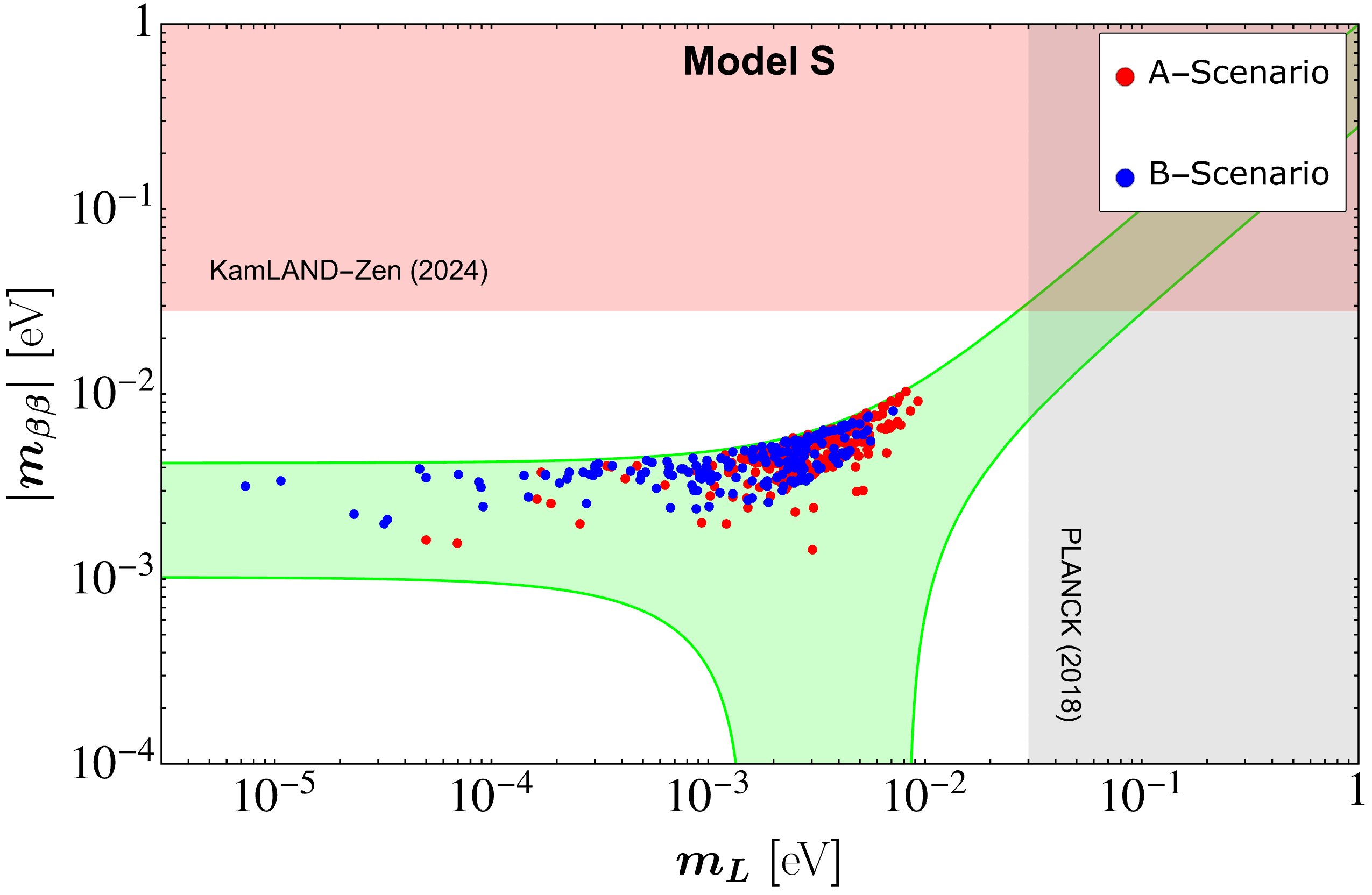
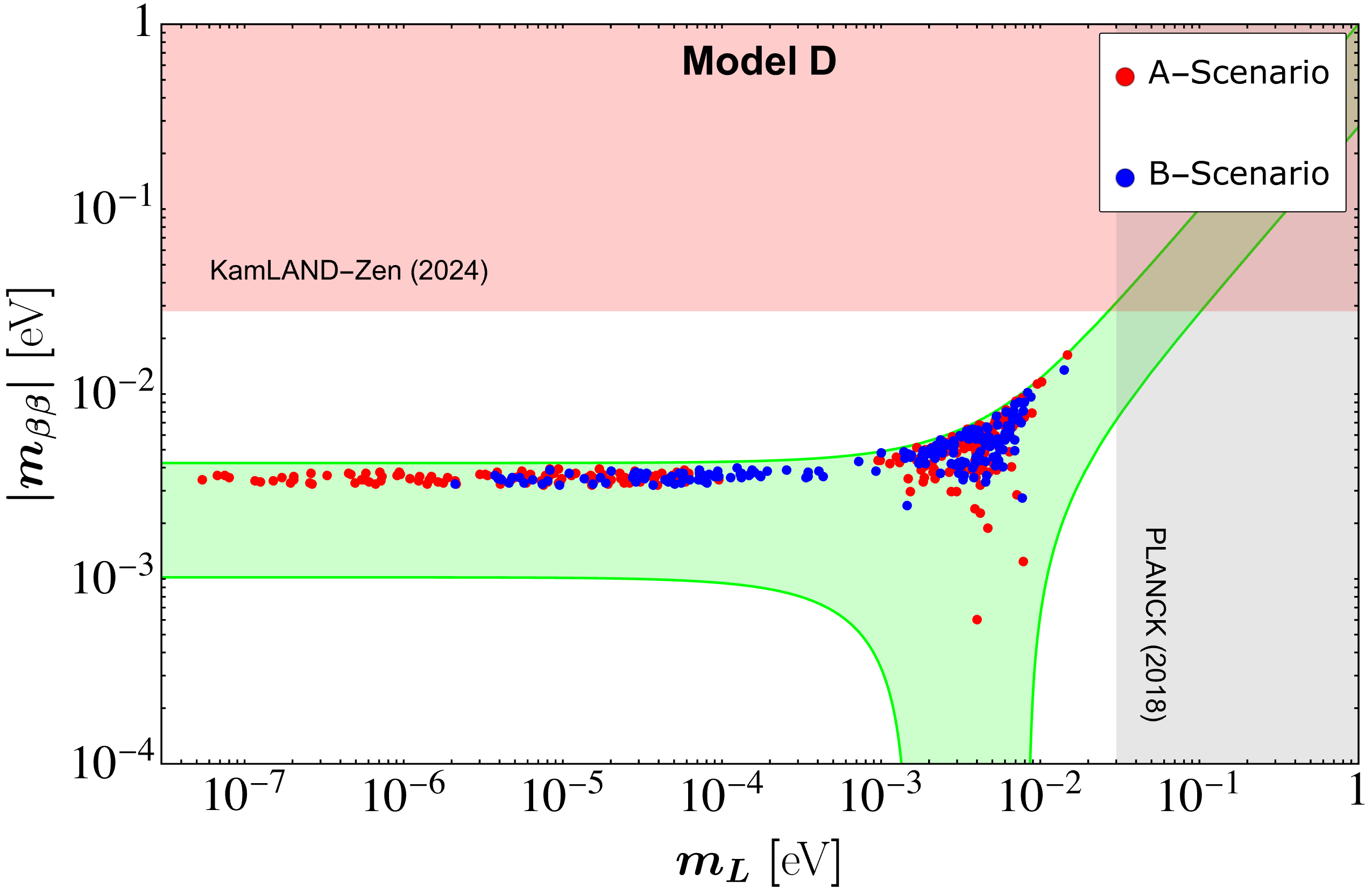
Figure 2: Distributions of the absolute value of $m_{\beta\beta}$ in terms of the lightest neutrino mass $m_{L}$. For each plot, all the valid representations for the viable patterns belonging to the given Model are collected, with a red or blue point, respectively, for Scenario A or B. The green zone corresponds to the $3\sigma$ confidence region for NO. The red exclusion region corresponds to the latest KamLAND-Zen upper limit on $\lvert m_{\beta\beta}\rvert$ KamLAND-Zen:2024eml , while the grey exclusion region corresponds to the PLANCK 2018 upper limit on $m_{L}$ Planck:2018vyg ; DiValentino:2019dzu .

If we call representation a particular set of parameters $\{e_{ij},y_{ij},k_{ij}\}$, from which we can derive the corresponding mass matrix $m_{\nu}^{M}$ and PMNS matrix $U$, we define such a representation as valid if it reproduces the six observables of Table 2 within the experimental $3\sigma$ ranges, which are taken from NuFIT 6.0 Esteban:2024eli using the dataset with SK atmospheric data. Each point in the two plots corresponds to a valid representation; the point is red for A-Scenario (see eq. (19)) or blue for B-Scenario (see eq. (20)). Each plot gathers the valid representations of all the viable patterns corresponding to the given Model (S or D). We can note from the plots that there are no points with $\lvert m_{\beta\beta}\rvert>20\ \text{meV}$. Currently, the most stringent experimental constraint comes from KamLAND-Zen, which provides an upper bound on $\lvert m_{\beta\beta}\rvert$ of 28 meV at $90\%$ confidence level (CL) KamLAND-Zen:2024eml (see the red exclusion region in the two plots of Fig. 2). However, upcoming experiments, such as CUPID CUPID:2022jlk , LEGEND-1000 LEGEND:2021bnm and nEXO nEXO:2021ujk , aim to reach sensitivities beyond $10\ \text{meV}$. In particular, the nEXO experiment is designed to reach an upper limit on $\lvert m_{\beta\beta}\rvert$ down to 4.7 meV, which nonetheless is not enough to probe most of the possible $\lvert m_{\beta\beta}\rvert$ obtainable in our models.

In Fig. 2 we can also see an upper bound on the lightest mass $m_{L}$ (grey exclusion region), arising from PLANCK 2018 cosmology measurements combined with the Baryonic Acoustic Oscillations (BAO) data Planck:2018vyg ; DiValentino:2019dzu , which provide an upper bound $\sum_{i}m_{i}\leq 0.12\ \text{eV}$ at $95\%$ CL. This bound translates to the bound on the lightest neutrino mass, that is, for NO, $m_{L}\lesssim 30\ \text{meV}$. These bounds will be improved by the combination of the future experiment results on CMB, galaxy surveys and dark matter measurements. Some examples are given by CMB-S4 CMB-S4:2016ple ; Calabrese:2016eii ; Dvorkin:2022bsc , CORE CORE:2016npo , EUCLID Audren:2012vy ; Sprenger:2018tdb , the Large Synoptic Survey Telescope (LSST) LSST:2008ijt , DESI Font-Ribera:2013rwa ; DESI:2024mwx and the Square Kilometre Arrey (SKA) Zegeye:2024jdc . These future experiments may be able to probe smaller masses; however, it is difficult to provide a precise estimate of the future upper bounds on $\sum_{i}m_{i}$ since these results strongly depend on the cosmological model. An example is given by DESI:2025ejh , where the new DESI measures provide negative neutrino masses as the best-fit values. This is a strong indication that the cosmological model used to derive those values may be incorrect.

If we look at the Model D plot (upper panel in Fig. 2), there is a tail disconnected from the point cluster in both Scenarios. This tail reaches very small values of the lightest mass $m_{L}$. For the Model D patterns with A-Scenario (red points), this tail is due to the D3 A and D4 A patterns. As already mentioned, these two patterns have some Majorana parameters forced to take small values, and this constraints lead to very low $m_{L}$ (some points in the plot reach $m_{L}<10^{-7}\ \text{eV}$). We can therefore say that patterns D3 A and D4 A, which in Linster:2018avp are not considered compatible with the observables, are able to reproduce the experimental data at the cost of forcing the value of some Majorana parameters. As a consequence, these patterns predict very small values of the lightest mass $m_{L}$. In a similar fashion, it can be found that the tail for Scenario B (the blue points in Fig. 2) is due to the pattern D5 B. In this case, however, the $m_{L}$ values do not fall below $10^{-6}\ \text{eV}$.

It is also interesting to note that, disregarding the tail of Model D, the cluster of points is slightly more dispersed for Model S patterns (bottom panel in Fig. 2). This is due to the fact that Model S has two more free parameters than Model D.

3.4.2 Predictions on $m_{\beta}$

We now turn our interests on the effective electron neutrino mass $m_{\beta}$, which determines the endpoint of the beta decay spectrum. This parameter is defined in the following way Franklin:2018adt :

$$m_{\beta}=\sqrt{\sum_{i}\lvert U_{ei}\rvert^{2}m_{i}^{2}}\ .$$ (26)

The best constraint comes from KATRIN experiment, which investigates the kinematics of the tritium beta spectrum near its kinematical endpoint Katrin:2024tvg . In Fig. 3 we report our results for $m_{\beta}$ versus $m_{L}$ for both Model S and Model D viable patterns.

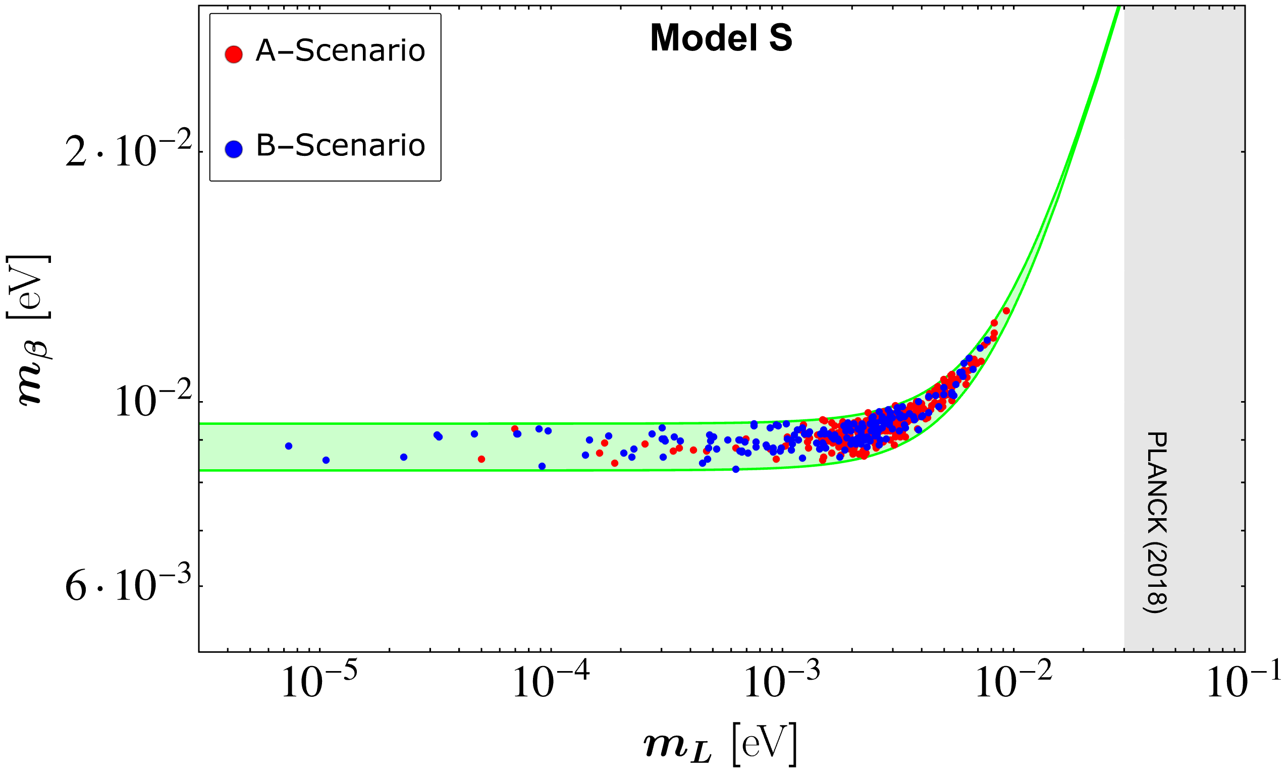
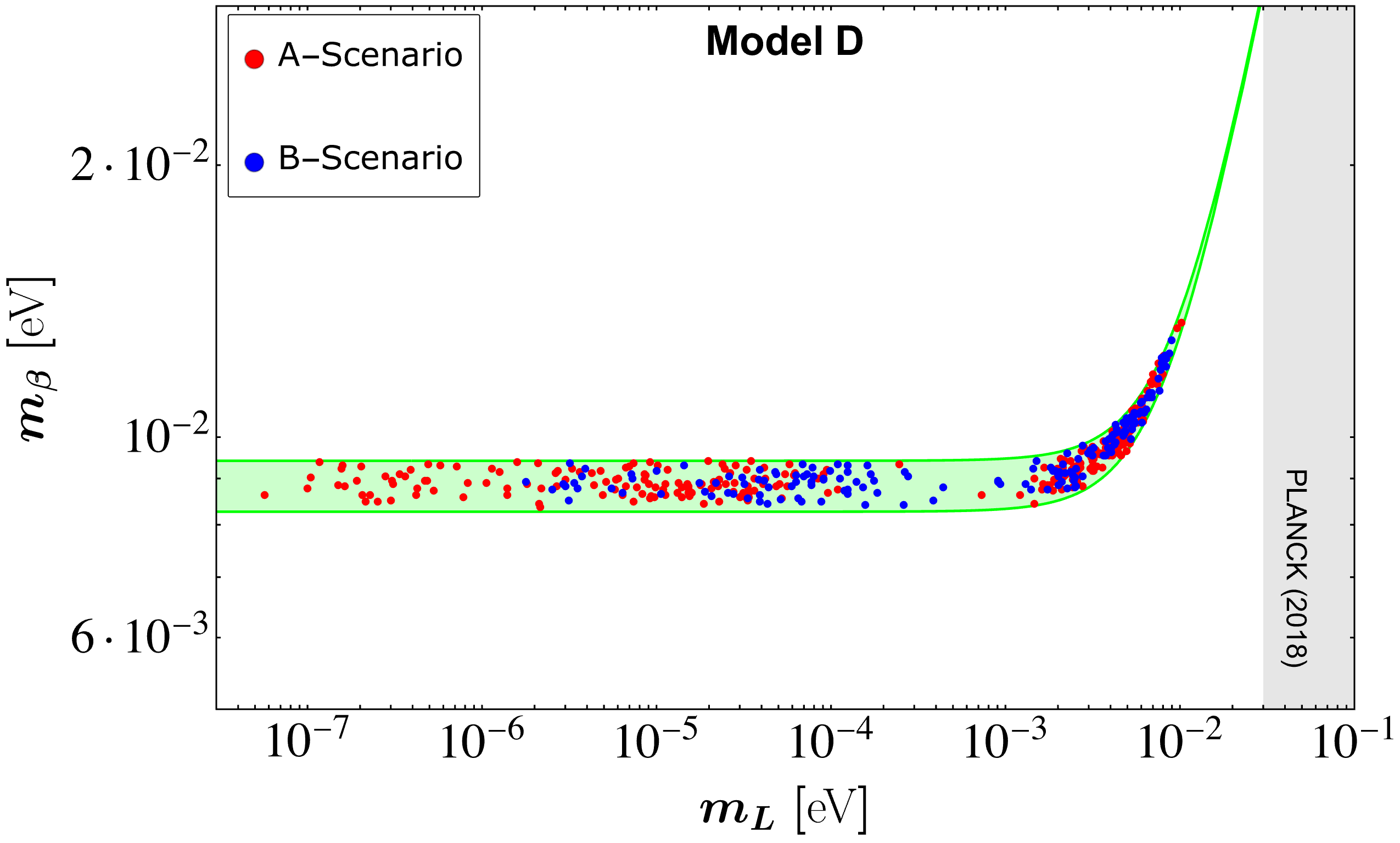
Figure 3: Distribution of $m_{\beta}$ in terms of the lightest neutrino mass $m_{L}$. For each plot, all the valid representations for the viable patterns belonging to the given Model are collected, with a red or blue point, respectively, for Scenario A or B. The green zone corresponds to the $3\sigma$ confidence region for NO, while the grey exclusion region corresponds to the PLANCK 2018 upper limit on $m_{L}$ Planck:2018vyg ; DiValentino:2019dzu .

Also in this case, each point corresponds to a particular valid representation (red for A-Scenario and blue for B-Scenario). From the two plots, it emerges that all the $m_{\beta}$ predictions are below 20 meV, a value significantly lower than the KATRIN upper bound $m_{\beta}<450\ \text{meV}$ (at $90\%$ CL), which is not shown in the plots. There are some interesting experiments in the pipeline. The most important are the Project 8 experiment Project8:2022wqh , which aims to reach the sensitivity of 40 meV for $m_{\beta}$, and the ECHo Gastaldo:2013wha ; Mantegazzini:2023igy and HOLMES experiments Alpert:2014lfa ; HOLMES:2016spk , which exploit the electron capture of ${}^{163}\text{Ho}$ and are expected to reach a sensitivity to $m_{\beta}$ on the order of 100 meV. The grey exclusion region in the two plots corresponds to the PLANCK 2018 upper bound ($m_{L}\lesssim 30\ \text{meV}$), which we have already discussed in Section 3.4.1.

The disconnected tail at very low values of $m_{L}$ in the Model D plot (bottom panel in Fig. 3) is caused by the same patterns discussed for the case of $\lvert m_{\beta\beta}\rvert$.

4 LFV decays and the muon anomalous magnetic moment

The electric and magnetic dipole moments offer valuable low-energy insights into potential New Physics (NP) beyond the Standard Model. Over the years, the long-standing tension in the anomalous magnetic moment of the muon $a_{\mu}=(g-2)_{\mu}/2$ has emerged as one the most compelling probe of NP. Recently, a new measurement at Fermilab has been reported using data collected in Run-2 and Run-3, in 2019 and 2020, respectively Muong-2:2023cdq . Systematic uncertanties were reduced by more than a factor of two compared to both the earlier E989 measurements at Fermilab Muong-2:2021ojo and the previous results from BNL Muong-2:2006rrc . Also, a complementary strategy to the Fermilab experiment based on ultracold muons is being pursued at J-PARC Razuvaev:2017uty ; Otani:2018kpl .

The latest measurements reveal a 5.1$\sigma$ discrepancy with the SM prediction $a_{\mu}^{\text{SM}}$ Muong-2:2023cdq ; Muong-2:2021ojo ; Muong-2:2006rrc :

$$\Delta a_{\mu}=a_{\mu}^{\text{Exp}}-a_{\mu}^{\text{SM}}=(249\pm 49)\times 10^{-11}\,.$$ (27)

However, it must be noted that the SM prediction suffers from uncertainties; in order to maintain them under control, recent advances have included into the theory prediction the hadronic vacuum polarization Keshavarzi:2018mgv , hadronic light-by-light scattering Colangelo:2017fiz ; Blum:2019ugy and higher-order hadronic corrections Jegerlehner:2009ry . Further studies are expected to clarify these theoretical differences in the near future, confirming or not the existence of such an anomaly.

If the anomalous magnetic moment of the muon is due to some NP, its effects could manifest in the Lepton Flavor Violating (LFV) decay in the charged lepton sector. We consider the $\ell_{\alpha}\rightarrow\ell_{\beta}\gamma$ decays, among which the most severe constraint comes from the branching ratio $\mathcal{B}(\mu\to e\gamma)<4.2\times 10^{-13}\,(90\%\text{ C.L.})$ by the MEG experiment MEG:2016leq . Whereas, the current upper-bounds for $\mathcal{B}(\tau\to\mu\gamma)$ and $\mathcal{B}(\tau\to e\gamma)$ are $4.4\times 10^{-8}$ BaBar:2009hkt and $3.3\times 10^{-8}$ Belle:2021ysv , respectively. Assuming that new degrees of freedom lie above the electroweak scale and can be integrated out, we analyze the electric and magnetic dipole moments of leptons within the framework of the SM Effective Field Theory. In particular, we focus on LFV transitions by exploring two complementary scenarios. In the first, we impose the current experimental constraint on $(g-2)_{\mu}$, and show that in our models it is not possible to simultaneously satisfy this constraint and the stringent experimental bounds on the decays $\ell_{\alpha}\rightarrow\ell_{\beta}\gamma$. In the second scenario, we relax the assumption on $(g-2)_{\mu}$ and demonstrate that effective operators can account for LFV processes without violating existing experimental limits.

4.1 The leptonic dipole operator

If the SM is understood as an EFT valid at the electroweak scale, new higher-dimensional operators $\mathcal{O}^{(n)}_{i}$ should be considered in the Effective Lagrangian, suppressed by a high-energy scale $\Lambda$ (which is in general a different scale with respect to the cut-off scale introduced in Section 2):

$$\mathcal{L}_{\text{SMEFT}}=\mathcal{L}_{\text{SM}}+\left(\sum_{n=1}^{d}\sum_{i}\frac{\mathcal{C}^{(n)}_{i}}{\Lambda^{n-4}}\mathcal{O}^{(n)}_{i}+\text{H.c.}\right)\,,\quad\text{for}\,\,d>4\,,$$ (28)

where $n=5,\dots,d$ runs over the dimension of the effective operator labeled by $i=1,\dots$ and $\mathcal{C}^{(n)}_{i}$ are dimensionless Wilson Coefficients (WCs). Notice that we dropped the flavor structures in the WCs as well as in the effective operators; we will explicitly show them when needed in the following. Below the electroweak symmetry breaking, the LFV processes are dictated by the dimension-6 leptonic dipole operators given as (in the left-right basis):

$$\mathcal{O}^{(6)}_{LR}=\frac{v}{\sqrt{2}}\bar{E}_{L}\sigma^{\mu\nu}E_{R}F_{\mu\nu}\,,$$ (29)

where $E_{L}$ and $E_{R}$ denote three flavors of left-handed and right-handed leptons, respectively. Also, $F_{\mu\nu}$ is the electromagnetic field strength tensor and $v\simeq 246$ GeV denotes the VEV of the Higgs doublet $H$. The operator in eq. (29) encodes the source of lepton flavor violation that we want to study as arising from our model. Thus, the relevant dipole effective Lagrangian is:

$$\mathcal{L}_{\text{dipole}}=\frac{1}{\Lambda^{2}}\left(\mathcal{C}^{\prime}_{LR}\mathcal{O}^{(6)}_{LR}+\mathcal{C}^{\prime}_{RL}\mathcal{O}^{(6)}_{RL}\right)\,,\quad\quad{\mathcal{C}^{\prime}}^{\dagger}_{RL}=\mathcal{C}^{\prime}_{LR}=\begin{pmatrix}\mathcal{C}_{ee}^{\prime}&\mathcal{C}^{\prime}_{e\mu}&\mathcal{C}^{\prime}_{e\tau}\\ \mathcal{C}^{\prime}_{\mu e}&\mathcal{C}^{\prime}_{\mu\mu}&\mathcal{C}^{\prime}_{\mu\tau}\\ \mathcal{C}^{\prime}_{\tau e}&\mathcal{C}^{\prime}_{\tau\mu}&\mathcal{C}^{\prime}_{\tau\tau}\end{pmatrix}\,,$$ (30)

where the prime of the WCs means that we are working in the mass-eigenstate basis of the charged leptons. The anomalous magnetic moment of the charged lepton $\ell$ can be written at the tree level in terms of the WCs of the dipole operator as follows:

$$\Delta a_{\ell}=\frac{4m_{\ell}}{e}\frac{v}{\sqrt{2}}\frac{1}{\Lambda^{2}}\Re\left[\mathcal{C}^{\prime}_{\ell\ell}\right]\,.$$ (31)

Then, using the input value $\Delta a_{\mu}=249\times 10^{-11}$ we obtain:

$$\frac{1}{\Lambda^{2}}\Re\left[\mathcal{C}^{\prime}_{\mu\mu}\right]=1.0\times 10^{-5}\text{ TeV}^{-2}\,.$$ (32)

On the other hand, the tree-level expression of the radiative LFV Branching Ratio (BR) reads:

$$\mathcal{B}\left(\ell_{\alpha}\rightarrow\ell_{\beta}\gamma\right)=\frac{m^{3}_{\ell_{\alpha}}\,v^{2}}{8\pi\Gamma_{\ell_{\alpha}}}\frac{1}{\Lambda^{4}}\bigg{(}|\mathcal{C}^{\prime}_{\alpha\beta}|^{2}+|\mathcal{C}^{\prime}_{\beta\alpha}|^{2}\bigg{)}\,,$$ (33)

where $\Gamma_{\ell_{\alpha}}$ is the total decay width of the lepton $\ell_{\alpha}$. Thus, using the current upper bounds from the latest experiments on the LFV processes listed in Table 4, it is possible to obtain the upper bounds of the Wilson Coefficients. The most stringent bound comes from the $\mu\rightarrow e\gamma$ and it gives:

$$\frac{1}{\Lambda^{2}}\Re\left[\mathcal{C}^{\prime}_{e\mu(\mu e)}\right]=2.1\times 10^{-10}\text{ TeV}^{-2}\,,$$ (34)

while, from branching ratios of the other LFV decays $\tau\rightarrow\mu\gamma$ and $\tau\rightarrow e\gamma$, we obtain:

$$\frac{1}{\Lambda^{2}}\Re\left[\mathcal{C}^{\prime}_{\mu\tau(\tau\mu)}\right]=2.65\times 10^{6}\text{ TeV}^{-2}\,,\quad\frac{1}{\Lambda^{2}}\Re\left[\mathcal{C}^{\prime}_{e\tau(\tau e)}\right]=2.35\times 10^{6}\text{ TeV}^{-2}\,,$$ (35)

respectively.

Observables	Exp.-SM/Bound	Wilson Coef. in $1/\Lambda^{2}$ $[\textbf{TeV}^{-2}$]
$\Delta a_{\mu}$	$249\times 10^{-11}$ Muong-2:2023cdq ; Muong-2:2021ojo ; Muong-2:2006rrc	$\Re\left[C^{\prime}_{\mu\mu}\right]=1.0\times 10^{-5}$
$\mathcal{B}(\mu\rightarrow e\gamma)$	$<4.2\times 10^{-13}$ MEG:2016leq	$|C^{\prime}_{e\mu\,(\mu e)}|<2.1\times 10^{-10}$
$\mathcal{B}(\tau\rightarrow\mu\gamma)$	$<4.2\times 10^{-8}$ BaBar:2009hkt ; Belle:2021ysv	$|C^{\prime}_{\mu\tau\,(\tau\mu)}|<2.65\times 10^{-6}$
$\mathcal{B}(\tau\rightarrow e\gamma)$	$<3.3\times 10^{-8}$ BaBar:2009hkt ; Belle:2021ysv	$|C^{\prime}_{e\tau\,(\tau e)}|<2.35\times 10^{-6}$

Table 4: Relevant observables and their current upper bounds from the latest experiments. In the last column the corresponding values of the Wilson coefficients presented in $1/\Lambda^{2}\left(\text{TeV}^{-2}\right)$ unit.

In our analysis, we consider the WC to be evaluated at the weak scale, neglecting the small effect of running below that scale Buttazzo:2020ibd . In the third column of Table 4, we report the values of the Wilson coefficients (in units of $1/\Lambda^{2}$ $[\text{TeV}^{-2}]$) corresponding to the upper bounds of the considered LFV processes.

4.2 Numerical analyses

Let us discuss the dipole operator in our model. Since in the SMEFT approach the low-energy predictions will not depend on the transformation properties of the flavons under the $U(2)_{F}$, our analyses will only be about the difference between the A-Scenario and B-Scenario, i.e. we will distinguish the models only by the value of the symmetry breaking parameters $\epsilon_{\phi}$ and $\epsilon_{\chi}$.

The flavor structure of the dipole operator is the same as the Yukawa matrix in eq. (4), which is diagonalized by the unitary transformation $U_{L}^{\dagger}YU_{R}$. The unitary matrices can be parametrized as

$$U_{L(R)}=U_{L(R)}^{23}\,U_{L(R)}^{13}\,U_{L(R)}^{12}\,,$$ (36)

and the rotations are given by:

$$U^{12}=\begin{pmatrix}c_{12}&s_{12}&0\\ -s_{12}&c_{12}&0\\ 0&0&1\end{pmatrix}\,,\quad U^{13}=\begin{pmatrix}c_{13}&0&s_{13}\\ 0&1&0\\ -s_{13}&0&c_{13}\end{pmatrix}\,,\quad U^{23}=\begin{pmatrix}1&0&0\\ 0&c_{23}&s_{23}\\ 0&-s_{23}&c_{23}\end{pmatrix}\,,$$ (37)

where $c_{ij}=\cos\theta_{ij}$ and $s_{ij}=\sin\theta_{ij}$. Also, notice that in general the mixing matrices $U_{L,R}$ would contain three phases (one for each rotation). However, since in our model the charged lepton Yukawa matrix is chosen to be real, such phases are irrelevant (inserting a CP-violation source in the charged lepton sector and then considering non-zero phases in the $U_{L,R}$ matrices would not change our results.)

In the mass-eigenstate basis of the charged leptons, the Wilson Coefficients associated with the dipole operator will be $\mathcal{C}^{\prime}_{\alpha\beta}=(U_{L}^{\dagger}\,\mathcal{C}\,U_{R})_{\alpha\beta}$. The predictions on the LFV processes will depend on the flavor structure of the dipole operator which directly originates from the $U(2)_{F}$ flavor symmetry, from the unitary matrices $U_{L,R}$ which are determined according to the best-fit analyses presented in Sec. 3.2 and from the numerical values of the Wilson Coefficient, that must to be understood as free parameters of the theory. In our numerical analyses the latter are extracted uniformly in the $[\lambda,\lambda^{-1}]$ range. Also, for the sake of simplicity, we assume them to be real, since our results will not depend on the imaginary part of the WCs.

4.2.1 Predictions of the $(g-2)_{e,\tau}$

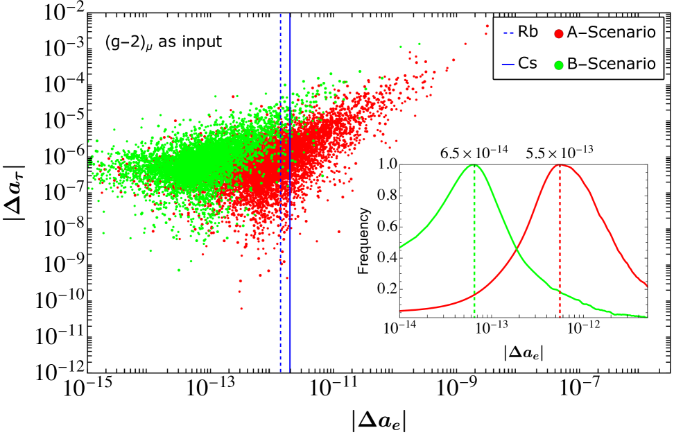
Figure 4: Correlations among $|\Delta a_{e}|$ and $|\Delta a_{\tau}|$ arising in the A-Scenario (B-Scenario) and represented with red (green) points, obtained considering the reference value for the anomalous magnetic moment as listed in Table 4. The numerical analysis is done assigning random values to the Wilson Coefficients in the $[\lambda,\lambda^{-1}]$ interval. In solid (dashed) blue line the 3$\sigma$ bound for the expected deviation from the SM prediction of the electron magnetic moment according to the latest observations based on Cesium (Rubidium) atomic recoil experiments. In the inset, with the same color code, we show the frequency distributions of the value of $\Delta a_{e}$ in A-Scenario and B-Scenario. See the main text for further details.

Let us assume that the dipole operator is responsible for the observed $(g-2)_{\mu}$. Thus, we impose the input value listed in Table 4 for the $\mathcal{C}_{\mu\mu}^{\prime}$ and we discuss the electron and the $\tau$ anomalous magnetic moments in our models.

The latest measurements of $(g-2)_{e,\tau}$ Hanneke:2008tm give

$$a_{e}^{\text{exp}}=1159652180.73(28)\times 10^{-12}\,,$$ (38)

and this must be compared to the SM prediction which strongly depends on the input value of the fine-structure constant $\alpha$. The latest two measurements based on the Rubidium Morel:2020dww and Cesium Parker:2018vye atomic recoil experiments are in a significant tension, despite being both compatible with the SM prediction within $1\sigma$ and $2.5\sigma$, respectively:

$$\Delta a_{e}^{\text{Rb}}=a_{e}^{\text{exp}}-a_{e}^{\text{SM,Rb}}= \,(+8\pm 0)\times 0^{-13}\,,$$ (39)

$$\Delta a_{e}^{\text{Cs}}=a_{e}^{\text{exp}}-a_{e}^{\text{SM,Cs}}= \,(-8\pm 6)\times 0^{-13}\,.$$

The aforementioned tension arises mostly due to their opposite signs. However, our model does not favor one sign over the other and, for this reason, we will focus only on the absolute value of the electron magnetic moment. The ratios of the diagonal components of the Wilson Coefficients in the A-Scenario and B-Scenario are (up to $\mathcal{O}\left(\lambda^{4}\,\sqrt{m_{e}/m_{\mu}}\right)$):

$$\textbf{A-Scenario}\,, \left|\frac{\mathcal{C}^{\prime}_{ee}}{\mathcal{C}^{\prime}_{\mu\mu}}\right|\sim\frac{m_{e}}{m_{\mu}}\left(1+2\sqrt{\frac{m_{\mu}}{m_{e}}}\frac{\sqrt{\cos{\theta_{23}^{L}}}}{\sin{\theta_{23}^{R}}}\frac{\mathcal{C}_{e\mu}\lambda^{2}}{\left(\cos{\theta_{23}^{L}\mathcal{C}_{\mu\tau}-\sin{\theta_{23}^{R}\mathcal{C}_{\tau\tau}}}\right)}\right)\,,$$ (40)

$$\textbf{B-Scenario}\,, \left|\frac{\mathcal{C}^{\prime}_{ee}}{\mathcal{C}^{\prime}_{\mu\mu}}\right|\sim\frac{m_{e}}{m_{\mu}}\left(1-\frac{\left(1-\cos{\theta_{23}^{R}}\right)\mathcal{C}_{\mu\mu}\lambda^{2}}{\sin{\theta_{23}^{R}}\mathcal{C}_{\tau\tau}}\right)\,,$$

where $\theta_{23}^{L}$ and $\theta_{23}^{R}$ are the mixing angles contained in the $U_{L}$ and $U_{R}$ unitary matrices, respectively. Both the A- and B-Scenarios agree on the prediction of the ratio $|\mathcal{C}^{\prime}_{ee}/\mathcal{C}^{\prime}_{\mu\mu}|\sim m_{e}/m_{\mu}$ at the Leading Order (LO), but it is evident that the Next-To-Leading Order (NLO) contribution in the A-Scenario is enhanced by a multiplicative factor $\sqrt{m_{\mu}/m_{e}}$. This implies that the A-Scenario predicts a generally bigger $|\Delta a_{e}|$ compared to the B-Scenario. This is evident in Fig. 4, where the $|\Delta a_{e}|\text{ vs }|\Delta a_{\tau}|$ is shown. We performed a scan on the WCs extracting their modulus flat in $[\lambda,\lambda^{-1}]$, with the red (green) points referring to A-Scenario (B-Scenario) predictions. The solid (dashed) vertical blue lines refer to the $3\sigma$ upper bounds for the $|\Delta a_{e}|$ from the latest experiments based on Cesium (Rubidium) atomic recoils. It is evident that the B-Scenario predicts a smaller value of $|\Delta a_{e}|$, while the predictions of $|\Delta a_{\tau}|$ do not manifest any difference between the two classes of models. In order to understand what the preferred predicted value of $\Delta a_{e}$ in each scenario is, we show its frequency distribution in the inset plot of Fig. 4. We normalized the frequency distribution to 1 and show it for both A and B scenarios, in red and green, respectively. The values corresponding to the peak of the distributions are:

$$\textbf{\small{{A-Scenario}}}: \Delta a_{e}=\frac{4m_{e}}{e}\frac{v}{\sqrt{2}}\frac{1}{\Lambda^{2}}\Re[\mathcal{C}^{\prime}_{ee}]\simeq 5\times 0^{-13}\,,$$ (41)

$$\textbf{\small{{B-Scenario}}}: \Delta a_{e}=\frac{4m_{e}}{e}\frac{v}{\sqrt{2}}\frac{1}{\Lambda^{2}}\Re[\mathcal{C}^{\prime}_{ee}]\simeq 0\times 0^{-14}\,.$$

It is worth to mention that the predicted values are inside the current $3\sigma$ upper bounds and, for this reason, it is not possible to test our models of flavor at present. A similar analysis for $\Delta a_{\tau}$ gives:

$$\Delta a_{\tau}=\frac{4m_{\tau}}{e}\frac{v}{\sqrt{2}}\frac{1}{\Lambda^{2}}\Re[\mathcal{C}^{\prime}_{\tau\tau}]\simeq 6.9\times 10^{-7}\,,$$ (42)

for both the scenarios. Due to the lack of more precise measurements, we cannot use this prediction to test our models.

Notice that, for both the electron and tau anomalous magnetic moments, our results are approximately in agreement with the naive scaling $\Delta a_{\ell}\approx m_{\ell}^{2}$ Giudice:2012ms , even though the presence of the additional $U(2)_{F}$ flavor symmetry introduces slight deviations.

4.2.2 LFV decays $\ell_{\alpha}\rightarrow\ell_{\beta}\gamma$ in light of $(g-2)_{\mu}$

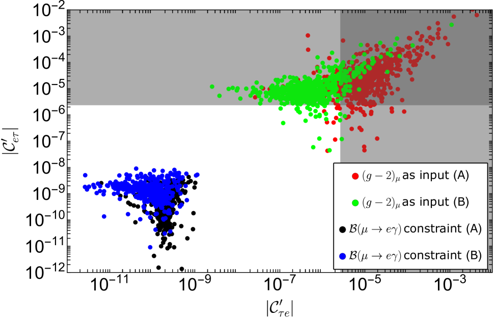
Figure 5: $\big{|}\mathcal{C}^{\prime}_{e\tau}\big{|}$ in $1/\Lambda^{2}[\text{TeV}^{-2}]$ unit versus $\big{|}\mathcal{C}^{\prime}_{\tau e}\big{|}$. The dark grey region is excluded by the experiments. In red (green) the predictions in the A-Scenario (B-Scenario) in light of the $(g-2)_{\mu}$. In black (blue) the predictions in the A-Scenario (B-Scenario) relaxing the requirement to reproduce the current $(g-2)_{\mu}$ value and using the current upper bound $\mathcal{B}(\mu\rightarrow e\gamma)$ as a constraint.

The NP responsible for the observed anomalous magnetic moment of the muon could manifest in LFV decays. In the following, we will investigate the predictions of LFV decays in our model in light of the $(g-2)_{\mu}$, whose most severe bound comes from the MEG experiment $\mathcal{B}(\mu\rightarrow e\gamma)<4.2\times 10^{-13}$ MEG:2016leq .

The relevant WC ratios are:

1. 
   

   $$\bigg{|}\frac{\mathcal{C}^{\prime}_{e\mu}}{\mathcal{C}^{\prime}_{\mu\mu}}\bigg{|}\sim \frac{1}{\sqrt{\cos\theta_{23}^{L}}}\sqrt{\frac{m_{e}}{m_{\mu}}}+\cot{\theta_{23}^{R}}\frac{\mathcal{C}_{e\mu}\lambda^{2}}{\cos{\theta_{23}^{L}}\mathcal{C}_{\mu\tau}-\sin{\theta_{23}^{L}}\mathcal{{C}_{\tau\tau}}}+\mathcal{O}(\lambda^{4})\,,$$ (43)

   $$\bigg{|}\frac{\mathcal{C}^{\prime}_{\mu e}}{\mathcal{C}^{\prime}_{\mu\mu}}\bigg{|}\sim \sqrt{\cos\theta_{23}^{L}}\sqrt{\frac{m_{e}}{m_{\mu}}}+\cot{\theta_{23}^{R}}\frac{\mathcal{C}_{e\mu}\lambda^{2}}{\cos{\theta_{23}^{L}}\mathcal{C}_{\mu\tau}-\sin{\theta_{23}^{L}}\mathcal{{C}_{\tau\tau}}}+\mathcal{O}(\lambda^{2}\sqrt{m_{e}/m_{\mu}})\,;$$

   
   

2. 
   

   $$\bigg{|}\frac{\mathcal{C}^{\prime}_{e\mu}}{\mathcal{C}^{\prime}_{\mu\mu}}\bigg{|}\sim \frac{1}{\sqrt{\cos\theta_{23}^{L}}}\sqrt{\frac{m_{e}}{m_{\mu}}}+\cot{\theta_{23}^{R}}\frac{\mathcal{C}_{e\mu}\lambda^{2}}{\cos{\theta_{23}^{L}}\mathcal{C}_{\mu\tau}-\sin{\theta_{23}^{L}}\mathcal{{C}_{\tau\tau}}}+\mathcal{O}(\lambda^{4})\,,$$ (44)

   $$\bigg{|}\frac{\mathcal{C}^{\prime}_{\mu e}}{\mathcal{C}^{\prime}_{\mu\mu}}\bigg{|}\sim \sqrt{\cos\theta_{23}^{L}}\sqrt{\frac{m_{e}}{m_{\mu}}}+\cot{\theta_{23}^{R}}\frac{\mathcal{C}_{e\mu}\lambda^{2}}{\cos{\theta_{23}^{L}}\mathcal{C}_{\mu\tau}-\sin{\theta_{23}^{L}}\mathcal{{C}_{\tau\tau}}}+\mathcal{O}(\lambda^{2}\sqrt{m_{e}/m_{\mu}})\,.$$

Our models do not manifest a suppression of $\mathcal{C}^{\prime}_{e\mu}$ compared with $\mathcal{C}^{\prime}_{\mu e}$. It means that even though the angular distribution with respect to the muon polarization can distinguish between $\mu_{R}\rightarrow e_{L}\gamma$ and $\mu_{L}\rightarrow e_{R}\gamma$ Okada:1999zk , this cannot be used to probe our models at present. Also, it is evident that assuming all the WCs to be of $\mathcal{O}(1)$, for both the A-Scenario and the B-Scenario the $\mathcal{C}^{\prime}_{e\mu(\mu e)}$ is suppressed by at most an $\mathcal{O}(10^{-2})$ with respect to $\mathcal{C}^{\prime}_{\mu\mu}$, which implies that $\mathcal{C}^{\prime}_{e\mu(\mu e)}\sim\mathcal{O}(10^{-7})$. Therefore, following eq. (33), the predicted $\mathcal{B}(\mu\rightarrow e\gamma)$ violates the current experimental upper bound listed in Table 4 by $2\div 3$ orders of magnitude. This is not surprising because the same NP couples similarly to the electron and muon BSM sectors so that

$$\mathcal{B}(\mu\rightarrow e\gamma)=\dfrac{\alpha m_{\mu}^{2}}{16m_{e}\Gamma_{\mu}}\big{|}\Delta a_{\mu}\Delta a_{e}\big{|}\,,$$ (45)

where $\alpha$ is the fine-structure constant and $\Gamma_{\mu}$ the total decay width of the muon.

Thus, using the anomalous magnetic moment of the muon as an input value together with the predicted $\Delta a_{e}$ in our models, a violation of the latest MEG bound on the $\mu\rightarrow e\gamma$ is unavoidable unless a fine-tuning on the WCs is invoked. Also, the predicted BRs of the radiative LFV decays $\tau\rightarrow e\gamma$ and $\tau\rightarrow\mu\gamma$ exceed the latest upper-bounds: $\mathcal{B}(\tau\to e\gamma)<4.4\times 10^{-8}$ BaBar:2009hkt and $\mathcal{B}(\tau\to\mu\gamma)<3.3\times 10^{-8}$ Belle:2021ysv . To keep the text readable, we leave the analytical expressions of the associated Wilson Coefficient ratios in Appendix A and we only present here the numerical results in Figs. 5 and 6. The absolute values of the relevant WCs in the A-Scenario and B-Scenario are shown in red and green circles, respectively.

It is evident that using the value of the $(g-2)_{\mu}$ anomaly as input, all models violate the latest upper bounds of the LFV decays involving tauons (listed in Table 4). On the other hand, we can relax the requirement to reproduce the anomalous magnetic moment of the muon and impose the condition that our models satisfy the most severe bound of $\mu\rightarrow e\gamma$. The result will be that the predicted $(g-2)_{e,\mu}$ are strongly suppressed according to the expected relation in eq. (45) and the SM predictions will be essentially recovered. In addition, the other LFV decays $\tau\rightarrow e\gamma$ and $\tau\rightarrow\mu\gamma$ rates will be predicted according to the latest upper bounds. This is shown in Figs. 5 and 6 where the black and blue circles represent the relevant absolute values of the WCs imposing the constraint $\mathcal{B}(\mu\rightarrow e\gamma)$ in the A-Scenario and B-Scenario, respectively.
It is important to highlight that, within an $U(2)_{F}$ flavor model, the current experimental limits on the branching ratios of LFV decays are not compatible with the observed $\Delta a_{\mu}$. This suggests that the current $(g-2)_{\mu}$ deviation from the Standard Model cannot be consistently explained unless the electron and muon sectors are effectively decoupled. This can be accomplished, for instance, by invoking UV completions. However, this is beyond the scope of this paper and we leave it for a possible follow-up study.

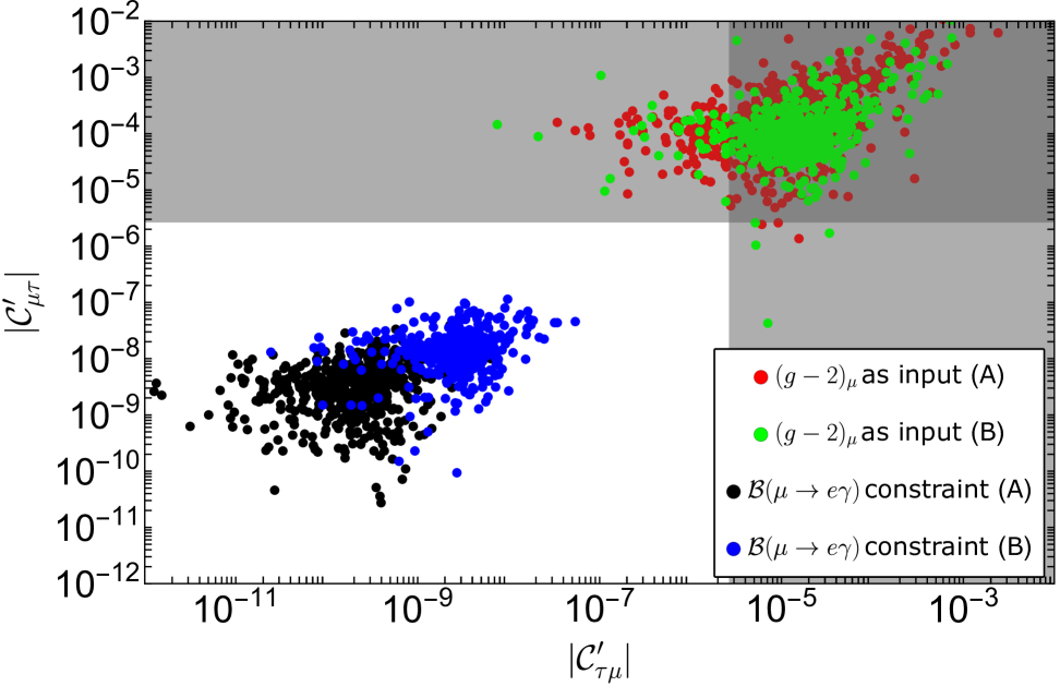
Figure 6: $\big{|}\mathcal{C}^{\prime}_{e\tau}\big{|}$ in $1/\Lambda^{2}[\text{TeV}^{-2}]$ unit versus $\big{|}\mathcal{C}^{\prime}_{\tau e}\big{|}$. The dark grey region is excluded by the experiments. The color code is the same as of Fig. 5.

5 Conclusions

The discovery of neutrino oscillations, and hence the fact that neutrinos are massive, has introduced a wide range of unanswered questions into particle physics. For this reason, it has become of fundamental importance to construct a flavor symmetry capable not only of predicting the mass spectrum across generations, but also of accounting for the mixing patterns of both neutrinos and quarks, which exhibit markedly different features. In this work, we wanted to extend to the neutrino sector the model presented in Linster:2018avp where an $U(2)_{F}$ flavor symmetry, isomorphic to $SU(2)_{F}\times U(1)_{F}$, has been proposed to predict quark and leptons masses and mixings with the introduction of two flavons: an $SU(2)_{F}$ doublet $\phi$ and a singlet $\chi$. Such a model failed to recover the observed neutrino mass spectrum via type-I see-saw when some assumptions on the quantum numbers of Majorana neutrinos under the flavor symmetry were made. We show that: a) relaxing the requirement that the $SU(2)_{F}$ structure of Majorana neutrino should reflect the $SU(2)_{F}$ structure of lepton doublets and b) allowing for them to assume also negative $U(1)_{F}$ charges, it is possible to fit all neutrinos and leptons observables successfully. In order to make a complete classification of all possible charge assignments, we distinguished three different classes of Models, depending on the $SU(2)_{F}$ structure of Majorana neutrinos:

• Model S: the three Majorana neutrinos are singlets under $SU(2)_{F}$

• Model D: two Majorana neutrinos ($N_{1}$ and $N_{2}$) are in a flavor doublet while $N_{3}$ is a singlet

• Model T: the three Majorana neutrinos transform as a flavor triplet.

Successively, using the see-saw type-I mechanism, we searched for all the possible light neutrino mass matrices scanning over the $U(1)_{F}$ charges of Majorana neutrinos. By considering mass matrix patterns as distinct when the difference between corresponding entries was at least of order $\lambda^{4}$ (with $\lambda\sim 0.2$) smaller than the leading term of that entry, we identified a total of 104 different patterns. We further classified them in A and B scenarios according on whether the flavons VEVs were considered of the same order of magnitude or hierarchical (that is, $\varepsilon_{\chi}/\varepsilon_{\phi}\sim\lambda$), respectively. Performing a fit on the neutrino observables (mixing angles and $\Delta m_{ij}^{2}$) as well as on the ratios of charged leptons masses, we found 13 patterns which reproduce all the observables in a satisfactory way with very low $\chi^{2}$ values and with a relatively small fine-tuning, estimated through the $d_{FT}$ parameter. For all unknown couplings, we left the modulus to vary in the range [$\lambda$, $\lambda^{-1}$] and the phases in the whole $[0,2\pi)$ range. Out of the 13 patterns, 6 were part of Model S (with two of them belonging to the B-Scenario) while 7 were part of the Model D (with 3 being of the B-Scenario category). No Model T patterns succeeded in the fit, due to small number of free parameters which introduced strong, unbreakable correlations among observables. The main conclusions derived from a detailed analysis of the 13 patterns are:

• All the viable patterns could reproduce only the Normal Ordering.

• With some particular choices of charges, anarchical neutrino mixing matrices were found. These particular patterns are known to be able to fit neutrino observable.

• The tentative choice for Majorana charges made in Linster:2018avp was discarded since, from analytical expressions, it could not reproduce the neutrino mass spectrum. However, their charge choice appeared in one of our 13 viable patterns. We demonstrated that, in this particular case, it is still possible to correctly reproduce the value of $\alpha=\Delta m_{21}^{2}/\Delta m^{2}_{31}$ by lowering only one parameter of the Majorana mass matrix to a value similar to $\lambda$. This feature has been observed also in other two viable patterns. The main consequence of this is the lowering of the predicted lightest neutrino mass down to $10^{-7}$ eV.

• All the viable patters predict an effective Majorana mass parameter $m_{\beta\beta}$ between $10^{-3}$ and $10^{-2}$ eV, which might be close to the reaches of future $0\nu\beta\beta$ experiments. On the other hand, the predicted effective neutrino mass $m_{\beta}$ is too low (less than 20 meV) to be reachable by current and next-generation experiments involving tritium decays or Holmium electron capture.

We further observed that, given the presence of unbounded and uncorrelated phases, our model could not predict any specific value of the PMNS CP-violating phase $\delta$.
In the final part of our study, we performed an analysis on the leptons dipole operators and on the LFV decays within the 13 selected patters. In particular, we assumed all the new physics mediating the processes to be integrated out and, in an EFT approach, we studied the predictions of our $U(2)_{F}$ models. We found out that, if we assume the $(g-2)_{\mu}$ anomaly as input for our analysis, then the predictions on the LFV process $\mu\to e\gamma$ are already excluded by current measurements. However, if we set the current bounds on $\mu\to e\gamma$ as input, we lower the prediction on $(g-2)_{\mu}$, setting consistent bounds on other processes like $\tau\to e\gamma$, $\tau\to\mu\gamma$ and on the electron and $\tau$ dipole moment. Therefore, if future theoretical calculations Keshavarzi:2018mgv ; Colangelo:2017fiz ; Blum:2019ugy ; Jegerlehner:2009ry or updated experimental analyses Muong-2:2015xgu will reduce the tension in the $(g-2)_{\mu}$ anomaly, our simple $U(2)_{F}$ flavor model could offer a fully consistent framework not only for explaining neutrino masses and mixing, but also for accommodating new physics capable of mediating LFV processes.

Acknoledgements

SM thanks C. Hagedorn for useful discussions and comments. SM acknowledges financial support from the project "consolidaciòn investigadora" CNS2022-13600.

Appendix A $(g-2)_{\mu}$ versus the LFV processes $\tau\rightarrow e\gamma$ and $\tau\rightarrow\mu\gamma$

In Sec. 4.2.2 we used the analytical expansions in eqs. (43,44) to affirm that, by using the $(g-2)_{\mu}$ value as an input for our numerical analysis, the upper-bound for the $\mu\rightarrow e\gamma$ is violated. In this Appendix we want to follow a similar reasoning for the LFV radiative decays of the tauons. Therefore, we present the correlations between the muon anomalous magnetic moment and the LFV radiative processes $\tau\rightarrow e\gamma$ and $\tau\rightarrow\mu\gamma$.

The ratios of the relevant WC are:

1. 
   

   $$\bigg{|}\frac{\mathcal{C}^{\prime}_{e\tau}}{\mathcal{C}^{\prime}_{\mu\mu}}\bigg{|}\sim \frac{\cot{\theta_{23}^{R}}}{\sqrt{\cos{\theta_{23}^{L}}}}\sqrt{\frac{m_{e}}{m_{\mu}}}+\frac{\mathcal{C}_{e\mu}\lambda^{2}}{\kappa}+\mathcal{O}(\lambda^{4})\,,$$ (46)

   $$\bigg{|}\frac{\mathcal{C}^{\prime}_{\tau e}}{\mathcal{C}^{\prime}_{\mu\mu}}\bigg{|}\sim \sqrt{\cos{\theta_{23}^{L}}}\sqrt{\frac{m_{e}}{m_{\mu}}}\left(\frac{\sin{\theta_{23}^{L}}\mathcal{C}_{\mu\tau}+\cos{\theta_{23}^{L}}\mathcal{C}_{\tau\tau}}{\kappa}\right)-\frac{\sin{\theta_{23}^{L}\mathcal{C}_{e\mu}\lambda^{2}}}{\sin{\theta_{23}^{R}}\kappa}+\mathcal{O}\left(\lambda^{2}\sqrt{m_{e}/m_{\mu}}\right)\,,$$

   $$\bigg{|}\frac{\mathcal{C}^{\prime}_{\mu\tau}}{\mathcal{C}^{\prime}_{\mu\mu}}\bigg{|}\sim \cot{\theta_{23}^{R}}+\left(\frac{\cos{\theta_{23}^{L}}\mathcal{C}_{\mu\mu}-\sin{\theta_{23}^{L}}\mathcal{C}_{\tau\mu}}{{\sin^{2}{\theta_{23}^{R}}}\kappa}\right)\lambda^{2}+\mathcal{O}\left(m_{e}/m_{\mu}\right)\,,$$

   $$\bigg{|}\frac{\mathcal{C}^{\prime}_{\tau\mu}}{\mathcal{C}^{\prime}_{\mu\mu}}\bigg{|}\sim \frac{\sin{\theta_{23}^{L}}\mathcal{C}_{\mu\tau}+\cos{\theta_{23}^{L}}\mathcal{C}_{\tau\tau}}{\kappa}+\cot{\theta_{23}^{R}}\left(\frac{\mathcal{C}_{\mu\tau}\mathcal{C}_{\tau\tau}-\mathcal{C}_{\mu\mu}\mathcal{C}_{\tau\tau}}{\kappa^{2}}\right)\lambda^{2}+\mathcal{O}\left(m_{e}/m_{\mu}\right)\,,$$

2. 
   

   $$\bigg{|}\frac{\mathcal{C}^{\prime}_{e\tau}}{\mathcal{C}^{\prime}_{\mu\mu}}\bigg{|}\sim \frac{\cot{\theta_{23}^{R}}}{\sqrt{\cos{\theta_{23}^{L}}}}\sqrt{\frac{m_{e}}{m_{\mu}}}+\mathcal{O}\left(\lambda^{2}\sqrt{m_{e}/m_{\mu}}\right)\,,$$ (47)

   $$\bigg{|}\frac{\mathcal{C}^{\prime}_{\tau e}}{\mathcal{C}^{\prime}_{\mu\mu}}\bigg{|}\sim \sqrt{\cos{\theta_{23}^{L}}}\tan{\theta_{23}^{L}}\sqrt{\frac{m_{e}}{m_{\mu}}}+\mathcal{O}\left(\lambda\sqrt{m_{e}/m_{\mu}}\right)\,,$$

   $$\bigg{|}\frac{\mathcal{C}^{\prime}_{\mu\tau}}{\mathcal{C}^{\prime}_{\mu\mu}}\bigg{|}\sim \cot{\theta_{23}^{R}}+\frac{\mathcal{C}_{\mu\mu}\,\lambda^{2}}{{\sin^{2}{\theta_{23}^{R}}}\mathcal{C}_{\mu\tau}}+\mathcal{O}(\lambda^{3})\,,$$

   $$\bigg{|}\frac{\mathcal{C}^{\prime}_{\tau\mu}}{\mathcal{C}^{\prime}_{\mu\mu}}\bigg{|}\sim \tan{\theta_{23}^{L}}+\frac{\mathcal{C}_{\tau\tau}\,\lambda\,\left(\cos{\theta_{23}^{L}\mathcal{C}_{\mu\tau}+\sin{\theta_{23}^{L}}\mathcal{C}_{\tau\tau}\,\lambda}\right)}{\mathcal{C}_{\mu\tau}^{2}}+\mathcal{O}(\lambda^{3})\,.$$

where $\kappa=(\sin{\theta_{23}^{L}}\mathcal{C}_{\tau\tau}-\cos{\theta_{23}^{L}}\mathcal{C}_{\mu\tau})$. The analytical expansions in eqs. (47,46) prove that, if we consider the $(g-2)_{\mu}$ as an input value, our models violate the latest upper-bounds (see Table 4) for the radiative LFV decays $\tau\rightarrow e\gamma$ and $\tau\rightarrow\mu\gamma$, as it is confirmed by the numerical analysis in Figs. 5 and 6.

Appendix B Fit results

The following two tables contain the best-fit parameters for the 13 viable patterns (6 for Model S and 7 for Model D). The complete procedure of the numerical fit is accurately reported in Section 3.2.

Pattern	S1 A	S2 A	S3 A	S4 A	S1 B	S2 B
$e_{11}$	-0.33	-3.25	2.98	-2.02	3.01	-4.34
$e_{12}$	-0.44	-0.88	-0.41	-0.59	-2.15	-3.27
$e_{13}$	4.09	3.81	-2.20	4.13	0.33	-1.04
$e_{22}$	4.11	-0.53	2.76	2.53	1.86	-2.96
$e_{23}$	-3.74	3.78	2.72	3.03	-0.93	-1.41
$e_{31}$	1.23	3.63	0.60	0.91	3.71	2.29
$e_{32}$	2.76	-3.90	3.99	3.57	1.07	-1.51
$e_{33}$	1.86	-0.28	0.82	0.39	2.52	3.27
$y_{11}$	1.31	-1.33	-3.31	-3.07	3.22	3.35
$y_{12}$	1.73	-3.55	-1.60	-2.02	-3.68	-3.95
$y_{13}$	1.03	2.15	-4.20	-4.04	-0.56	0.48
$y_{21}$	3.06	4.31	-3.39	-3.27	0.95	-3.71
$y_{22}$	-2.41	0.48	1.40	-0.38	3.85	1.53
$y_{23}$	2.93	1.15	-1.85	-2.96	-0.65	-2.78
$y_{31}$	-1.19	-3.00	-2.90	-2.13	-4.27	-4.24
$y_{32}$	3.66	-3.01	-0.52	0.41	2.77	0.36
$y_{33}$	0.34	-1.80	1.65	4.06	2.19	1.98
$k_{11}$	-1.21	1.09	-4.12	-1.66	4.19	0.29
$k_{12}$	1.81	1.33	0.42	4.06	-1.57	-1.71
$k_{13}$	-3.89	1.94	-0.24	0.78	1.66	-3.52
$k_{22}$	3.94	3.37	-1.57	-1.95	1.29	-2.85
$k_{23}$	-2.75	-3.58	4.01	0.38	2.60	0.73
$k_{33}$	1.09	1.55	-0.54	-1.35	-1.82	-2.89
$\sin^{2}{\theta_{12}}$	0.302	0.302	0.302	0.308	0.307	0.305
$\sin^{2}{\theta_{13}}$	0.0222	0.0225	0.0225	0.0219	0.0224	0.0222
$\sin^{2}{\theta_{23}}$	0.454	0.457	0.454	0.458	0.458	0.458
$\alpha$	0.0294	0.0292	0.0296	0.0294	0.0296	0.0295
$r_{12}$	0.0048	0.0048	0.0047	0.0048	0.0048	0.0048
$r_{23}$	0.0547	0.0561	0.0567	0.0565	0.0571	0.0563
$\chi^{2}$	0.24	0.45	0.64	0.70	0.34	0.23
$d_{\text{FT}}$	7.12	4.19	12.2	6.02	5.53	5.72
$\chi^{2}+\text{P}_{\mathrm{MG}}$	27.00	26.62	26.22	25.97	24.19	29.04

Table 5: Best-fit values and fit parameters for Model S viable patterns. For the parameters $e_{ij}$, $y_{ij}$ and $k_{ij}$ we reported only the real part of their best-fit values.

Pattern	D1 A	D2 A	D3 A	D4 A	D1 B	D2 B	D5 B
$e_{11}$	1.00	-1.47	0.92	-3.18	1.69	0.94	-0.74
$e_{12}$	-0.32	-0.53	0.34	-0.31	-2.69	3.38	-1.28
$e_{13}$	0.62	-1.76	-2.15	3.60	2.15	0.89	1.95
$e_{22}$	-3.30	-3.01	3.18	0.92	-3.81	-2.33	-1.83
$e_{23}$	-2.67	3.10	-2.24	-2.40	1.19	-1.40	0.50
$e_{31}$	-2.06	-1.63	3.39	-3.94	-1.65	4.01	3.82
$e_{32}$	2.11	4.13	-3.88	2.65	-2.64	3.30	-3.68
$e_{33}$	-2.23	-0.65	-3.97	1.06	3.20	-2.77	2.61
$y_{11}$	2.36	-1.76	3.30	3.74	1.64	3.02	2.97
$y_{12}$	-1.02	0.76	2.86	-2.87	-2.72	3.29	-1.13
$y_{13}$	2.15	3.37	3.54	-3.98	0.36	0.42	-2.24
$y_{22}$	-3.05	3.89	-1.14	2.47	-1.61	-0.75	3.20
$y_{23}$	-1.11	-1.78	-2.58	-3.15	-2.56	2.08	3.28
$y_{31}$	-3.49	0.72	2.82	-0.38	-1.41	-3.40	3.32
$y_{32}$	3.44	-1.59	3.79	2.50	0.86	4.32	0.88
$y_{33}$	2.92	2.39	-0.42	-1.15	-3.64	1.02	1.26
$k_{11}$	1.61	3.55	-1.40	-1.61	3.21	4.05	2.10
$k_{12}$	-3.40	3.37	-3.92	-3.44	1.44	1.10	-3.50
$k_{13}$	-2.55	-3.41	2.31	3.76	0.39	-1.80	1.60
$k_{22}$	2.20	4.00	3.23	-1.59	1.86	3.67	-0.34
$k_{23}$	-0.95	3.05	0.28	-2.29	-0.62	0.77	1.12
$k_{33}$	3.65	0.56	1.82	-3.49	2.16	-2.11	-0.25
$\sin^{2}{\theta_{12}}$	0.297	0.305	0.305	0.297	0.300	0.305	0.303
$\sin^{2}{\theta_{13}}$	0.0221	0.0222	0.0221	0.0219	0.0223	0.0222	0.0222
$\sin^{2}{\theta_{23}}$	0.452	0.447	0.451	0.455	0.444	0.457	0.450
$\alpha$	0.0298	0.0295	0.0296	0.0304	0.0296	0.0298	0.0295
$r_{12}$	0.0048	0.0048	0.0048	0.0048	0.0048	0.0048	0.0048
$r_{23}$	0.0571	0.0577	0.0546	0.0569	0.0553	0.0570	0.0572
$\chi^{2}$	0.39	0.24	0.35	1.96	0.38	0.30	0.06
$d_{\text{FT}}$	17.1	7.03	37.6	4.26	8.41	3.31	45.0
$\chi^{2}+\text{P}_{\mathrm{MG}}$	24.44	27.71	28.10	28.43	19.97	22.33	22.07

Table 6: Best-fit values and fit parameters for Model D viable patterns. For the parameters $e_{ij}$, $y_{ij}$ and $k_{ij}$ we reported only the real part of their best-fit values.

References

- (1) Super-Kamiokande collaboration, Evidence for oscillation of atmospheric neutrinos, Phys. Rev. Lett. 81 (1998) 1562 [hep-ex/9807003].
- (2) M.K. Gaillard, P.D. Grannis and F.J. Sciulli, The Standard model of particle physics, Rev. Mod. Phys. 71 (1999) S96 [hep-ph/9812285].
- (3) E. Majorana, Teoria simmetrica dell’elettrone e del positrone, Nuovo Cim. 14 (1937) 171.
- (4) S.F. King and I.N.R. Peddie, Neutrino physics and the flavor problem, J. Korean Phys. Soc. 45 (2004) S443 [hep-ph/0312235].
- (5) F. Feruglio, Pieces of the Flavour Puzzle, Eur. Phys. J. C 75 (2015) 373 [1503.04071].
- (6) G. Abbas, R. Adhikari, E.J. Chun and N. Singh, The problem of flavour, Eur. Phys. J. Plus 140 (2025) 73 [2308.14811].
- (7) N. Cabibbo, Unitary Symmetry and Leptonic Decays, Phys. Rev. Lett. 10 (1963) 531.
- (8) M. Kobayashi and T. Maskawa, CP Violation in the Renormalizable Theory of Weak Interaction, Prog. Theor. Phys. 49 (1973) 652.
- (9) B. Pontecorvo, Mesonium and anti-mesonium, Sov. Phys. JETP 6 (1957) 429.
- (10) B. Pontecorvo, Inverse beta processes and nonconservation of lepton charge, Zh. Eksp. Teor. Fiz. 34 (1957) 247.
- (11) Z. Maki, M. Nakagawa and S. Sakata, Remarks on the unified model of elementary particles, Prog. Theor. Phys. 28 (1962) 870.
- (12) B. Pontecorvo, Neutrino Experiments and the Problem of Conservation of Leptonic Charge, Zh. Eksp. Teor. Fiz. 53 (1967) 1717.
- (13) P.F. Harrison, D.H. Perkins and W.G. Scott, Tri-bimaximal mixing and the neutrino oscillation data, Phys. Lett. B 530 (2002) 167 [hep-ph/0202074].
- (14) P.F. Harrison and W.G. Scott, Symmetries and generalizations of tri - bimaximal neutrino mixing, Phys. Lett. B 535 (2002) 163 [hep-ph/0203209].
- (15) Z.-z. Xing, Nearly tri bimaximal neutrino mixing and CP violation, Phys. Lett. B 533 (2002) 85 [hep-ph/0204049].
- (16) P.F. Harrison and W.G. Scott, mu - tau reflection symmetry in lepton mixing and neutrino oscillations, Phys. Lett. B 547 (2002) 219 [hep-ph/0210197].
- (17) P.F. Harrison and W.G. Scott, Permutation symmetry, tri - bimaximal neutrino mixing and the S3 group characters, Phys. Lett. B 557 (2003) 76 [hep-ph/0302025].
- (18) F. Feruglio and Y. Lin, Fermion Mass Hierarchies and Flavour Mixing from a Minimal Discrete Symmetry, Nucl. Phys. B 800 (2008) 77 [0712.1528].
- (19) G. Altarelli and F. Feruglio, Tri-bimaximal neutrino mixing from discrete symmetry in extra dimensions, Nucl. Phys. B 720 (2005) 64 [hep-ph/0504165].
- (20) F. Bazzocchi, L. Merlo and S. Morisi, Fermion Masses and Mixings in a S(4)-based Model, Nucl. Phys. B 816 (2009) 204 [0901.2086].
- (21) Daya Bay collaboration, Observation of electron-antineutrino disappearance at Daya Bay, Phys. Rev. Lett. 108 (2012) 171803 [1203.1669].
- (22) A. Giarnetti, S. Marciano and D. Meloni, On Quark–Lepton Mixing and the Leptonic CP Violation, Universe 10 (2024) 345 [2407.02487].
- (23) F. Feruglio, Are neutrino masses modular forms?, in From My Vast Repertoire …: Guido Altarelli’s Legacy, A. Levy, S. Forte and G. Ridolfi, eds., pp. 227–266 (2019), DOI [1706.08749].
- (24) F. Feruglio and A. Romanino, Lepton flavor symmetries, Rev. Mod. Phys. 93 (2021) 015007 [1912.06028].
- (25) T. Kobayashi, K. Tanaka and T.H. Tatsuishi, Neutrino mixing from finite modular groups, Phys. Rev. D 98 (2018) 016004 [1803.10391].
- (26) S. Marciano, D. Meloni and M. Parriciatu, Minimal seesaw and leptogenesis with the smallest modular finite group, JHEP 05 (2024) 020 [2402.18547].
- (27) T. Kobayashi, Y. Shimizu, K. Takagi, M. Tanimoto, T.H. Tatsuishi and H. Uchida, Finite modular subgroups for fermion mass matrices and baryon/lepton number violation, Phys. Lett. B 794 (2019) 114 [1812.11072].
- (28) J.C. Criado and F. Feruglio, Modular Invariance Faces Precision Neutrino Data, SciPost Phys. 5 (2018) 042 [1807.01125].
- (29) T. Kobayashi, N. Omoto, Y. Shimizu, K. Takagi, M. Tanimoto and T.H. Tatsuishi, Modular A4 invariance and neutrino mixing, JHEP 11 (2018) 196 [1808.03012].
- (30) H. Okada and M. Tanimoto, CP violation of quarks in modular invariance, Phys. Lett. B 791 (2019) 54 [1812.09677].
- (31) H. Okada and M. Tanimoto, Towards unification of quark and lepton flavors in modular invariance, Eur. Phys. J. C 81 (2021) 52 [1905.13421].
- (32) G.-J. Ding, S.F. King and X.-G. Liu, Modular A4 symmetry models of neutrinos and charged leptons, JHEP 09 (2019) 074 [1907.11714].
- (33) T. Asaka, Y. Heo, T.H. Tatsuishi and T. Yoshida, Modular invariance and leptogenesis, JHEP 01 (2020) 144 [1909.06520].
- (34) H. Okada, Y. Shimizu, M. Tanimoto and T. Yoshida, Modulus linking leptonic CP violation to baryon asymmetry in A4 modular invariant flavor model, JHEP 07 (2021) 184 [2105.14292].
- (35) T. Nomura, H. Okada and Y. Shoji, SU(4)C × SU(2)L× U(1)R models with modular A4 symmetry, PTEP 2023 (2023) 023B04 [2206.04466].
- (36) M.R. Devi, Retrieving texture zeros in 3+1 active-sterile neutrino framework under the action of modular-invariants, 2303.04900.
- (37) G.-J. Ding, S.F. King, X.-G. Liu and J.-N. Lu, Modular S4 and A4 symmetries and their fixed points: new predictive examples of lepton mixing, JHEP 12 (2019) 030 [1910.03460].
- (38) J.T. Penedo and S.T. Petcov, Lepton Masses and Mixing from Modular Symmetry, Nucl. Phys. B 939 (2019) 292 [1806.11040].
- (39) P.P. Novichkov, J.T. Penedo, S.T. Petcov and A.V. Titov, Modular S4 models of lepton masses and mixing, JHEP 04 (2019) 005 [1811.04933].
- (40) I. de Medeiros Varzielas, S.F. King and Y.-L. Zhou, Multiple modular symmetries as the origin of flavor, Phys. Rev. D 101 (2020) 055033 [1906.02208].
- (41) J.C. Criado, F. Feruglio and S.J.D. King, Modular Invariant Models of Lepton Masses at Levels 4 and 5, JHEP 02 (2020) 001 [1908.11867].
- (42) P.P. Novichkov, J.T. Penedo, S.T. Petcov and A.V. Titov, Modular A5 symmetry for flavour model building, JHEP 04 (2019) 174 [1812.02158].
- (43) G.-J. Ding, S.F. King and X.-G. Liu, Neutrino mass and mixing with modular symmetry, Phys. Rev. D 100 (2019) 115005 [1903.12588].
- (44) M. Leurer, Y. Nir and N. Seiberg, Mass matrix models, Nucl. Phys. B 398 (1993) 319 [hep-ph/9212278].
- (45) M. Leurer, Y. Nir and N. Seiberg, Mass matrix models: The Sequel, Nucl. Phys. B 420 (1994) 468 [hep-ph/9310320].
- (46) H.K. Dreiner and M. Thormeier, Supersymmetric Froggatt-Nielsen models with baryon and lepton number violation, Phys. Rev. D 69 (2004) 053002 [hep-ph/0305270].
- (47) S.T. Petcov, On Pseudodirac Neutrinos, Neutrino Oscillations and Neutrinoless Double beta Decay, Phys. Lett. B 110 (1982) 245.
- (48) G. Arcadi, S. Marciano and D. Meloni, Neutrino mixing and leptogenesis in a model, Eur. Phys. J. C 83 (2023) 137 [2205.02565].
- (49) M. Linster and R. Ziegler, A Realistic Model of Flavor, JHEP 08 (2018) 058 [1805.07341].
- (50) A. Falkowski, M. Nardecchia and R. Ziegler, Lepton Flavor Non-Universality in B-meson Decays from a U(2) Flavor Model, JHEP 11 (2015) 173 [1509.01249].
- (51) R. Barbieri, G.R. Dvali and L.J. Hall, Predictions from a U(2) flavor symmetry in supersymmetric theories, Phys. Lett. B 377 (1996) 76 [hep-ph/9512388].
- (52) R. Barbieri, L.J. Hall and A. Romanino, Consequences of a U(2) flavor symmetry, Phys. Lett. B 401 (1997) 47 [hep-ph/9702315].
- (53) E. Dudas, G. von Gersdorff, S. Pokorski and R. Ziegler, Linking Natural Supersymmetry to Flavour Physics, JHEP 01 (2014) 117 [1308.1090].
- (54) Muon g-2 collaboration, Measurement of the Positive Muon Anomalous Magnetic Moment to 0.20 ppm, Phys. Rev. Lett. 131 (2023) 161802 [2308.06230].
- (55) Muon g-2 collaboration, Measurement of the Positive Muon Anomalous Magnetic Moment to 0.46 ppm, Phys. Rev. Lett. 126 (2021) 141801 [2104.03281].
- (56) Muon g-2 collaboration, Final Report of the Muon E821 Anomalous Magnetic Moment Measurement at BNL, Phys. Rev. D 73 (2006) 072003 [hep-ex/0602035].
- (57) W. Buchmuller and D. Wyler, Effective Lagrangian Analysis of New Interactions and Flavor Conservation, Nucl. Phys. B 268 (1986) 621.
- (58) B. Grzadkowski, M. Iskrzynski, M. Misiak and J. Rosiek, Dimension-Six Terms in the Standard Model Lagrangian, JHEP 10 (2010) 085 [1008.4884].
- (59) R. Alonso, E.E. Jenkins, A.V. Manohar and M. Trott, Renormalization Group Evolution of the Standard Model Dimension Six Operators III: Gauge Coupling Dependence and Phenomenology, JHEP 04 (2014) 159 [1312.2014].
- (60) G. Panico, A. Pomarol and M. Riembau, EFT approach to the electron Electric Dipole Moment at the two-loop level, JHEP 04 (2019) 090 [1810.09413].
- (61) J. Aebischer, W. Dekens, E.E. Jenkins, A.V. Manohar, D. Sengupta and P. Stoffer, Effective field theory interpretation of lepton magnetic and electric dipole moments, JHEP 07 (2021) 107 [2102.08954].
- (62) L. Allwicher, P. Arnan, D. Barducci and M. Nardecchia, Perturbative unitarity constraints on generic Yukawa interactions, JHEP 10 (2021) 129 [2108.00013].
- (63) J. Kley, T. Theil, E. Venturini and A. Weiler, Electric dipole moments at one-loop in the dimension-6 SMEFT, Eur. Phys. J. C 82 (2022) 926 [2109.15085].
- (64) T. Kobayashi, H. Otsuka, M. Tanimoto and K. Yamamoto, Modular symmetry in the SMEFT, Phys. Rev. D 105 (2022) 055022 [2112.00493].
- (65) T. Kobayashi, H. Otsuka, M. Tanimoto and K. Yamamoto, Lepton flavor violation, lepton (g 2)μ,e and electron EDM in the modular symmetry, JHEP 08 (2022) 013 [2204.12325].
- (66) M. Tanimoto and K. Yamamoto, Electron EDM and LFV decays in the light of Muon with U(2) flavor symmetry, Eur. Phys. J. C 84 (2024) 252 [2310.16325].
- (67) T.A. Chowdhury and S. Nasri, Lepton Flavor Violation in the Inert Scalar Model with Higher Representations, JHEP 12 (2015) 040 [1506.00261].
- (68) A.S. De Jesus, S. Kovalenko, F.S. Queiroz, C. Siqueira and K. Sinha, Vectorlike leptons and inert scalar triplet: Lepton flavor violation, , and collider searches, Phys. Rev. D 102 (2020) 035004 [2004.01200].
- (69) S. Esch, M. Klasen, D.R. Lamprea and C.E. Yaguna, Lepton flavor violation and scalar dark matter in a radiative model of neutrino masses, Eur. Phys. J. C 78 (2018) 88 [1602.05137].
- (70) A. Giarnetti, J. Herrero-Garcia, S. Marciano, D. Meloni and D. Vatsyayan, Neutrino masses from new Weinberg-like operators: phenomenology of TeV scalar multiplets, JHEP 05 (2024) 055 [2312.13356].
- (71) A. Giarnetti, J. Herrero-García, S. Marciano, D. Meloni and D. Vatsyayan, Neutrino masses from new seesaw models: low-scale variants and phenomenological implications, Eur. Phys. J. C 84 (2024) 803 [2312.14119].
- (72) H. Georgi and S.L. Glashow, Unity of All Elementary Particle Forces, Phys. Rev. Lett. 32 (1974) 438.
- (73) Z. Liu and Y.-L. Wu, Leptonic CP Violation and Wolfenstein Parametrization for Lepton Mixing, Phys. Lett. B 733 (2014) 226 [1403.2440].
- (74) S. Roy, S. Morisi, N.N. Singh and J.W.F. Valle, The Cabibbo angle as a universal seed for quark and lepton mixings, Phys. Lett. B 748 (2015) 1 [1410.3658].
- (75) V. Brdar, A.J. Helmboldt, S. Iwamoto and K. Schmitz, Type-I Seesaw as the Common Origin of Neutrino Mass, Baryon Asymmetry, and the Electroweak Scale, Phys. Rev. D 100 (2019) 075029 [1905.12634].
- (76) I. Esteban, M.C. Gonzalez-Garcia, M. Maltoni, I. Martinez-Soler, J.a.P. Pinheiro and T. Schwetz, NuFit-6.0: updated global analysis of three-flavor neutrino oscillations, JHEP 12 (2024) 216 [2410.05380].
- (77) DUNE collaboration, Long-baseline neutrino oscillation physics potential of the DUNE experiment, Eur. Phys. J. C 80 (2020) 978 [2006.16043].
- (78) Hyper-Kamiokande collaboration, Hyper-Kamiokande Design Report, 1805.04163.
- (79) A. Alekou et al., The European Spallation Source neutrino super-beam conceptual design report, Eur. Phys. J. ST 231 (2022) 3779 [2206.01208].
- (80) ESSnuSB collaboration, The ESSnuSB Design Study: Overview and Future Prospects, Universe 9 (2023) 347 [2303.17356].
- (81) S.K. Agarwalla, S. Das, A. Giarnetti, D. Meloni and M. Singh, Enhancing sensitivity to leptonic CP violation using complementarity among DUNE, T2HK, and T2HKK, Eur. Phys. J. C 83 (2023) 694 [2211.10620].
- (82) P. Novichkov, Aspects of the Modular Symmetry Approach to Lepton Flavour, Ph.D. thesis, SISSA, Trieste, 2021.
- (83) S. Antusch, J. Kersten, M. Lindner and M. Ratz, Running neutrino masses, mixings and CP phases: Analytical results and phenomenological consequences, Nucl. Phys. B 674 (2003) 401 [hep-ph/0305273].
- (84) G. Altarelli and G. Blankenburg, Different Paths to Fermion Masses and Mixings, JHEP 03 (2011) 133 [1012.2697].
- (85) G. Altarelli and F. Feruglio, Models of neutrino masses and mixings, New J. Phys. 6 (2004) 106 [hep-ph/0405048].
- (86) L.J. Hall, H. Murayama and N. Weiner, Neutrino mass anarchy, Phys. Rev. Lett. 84 (2000) 2572 [hep-ph/9911341].
- (87) N. Haba and H. Murayama, Anarchy and hierarchy, Phys. Rev. D 63 (2001) 053010 [hep-ph/0009174].
- (88) G. Altarelli, F. Feruglio and I. Masina, Models of neutrino masses: Anarchy versus hierarchy, JHEP 01 (2003) 035 [hep-ph/0210342].
- (89) A. de Gouvea and H. Murayama, Statistical Test of Anarchy, Phys. Lett. B 573 (2003) 94 [hep-ph/0301050].
- (90) A. de Gouvea and H. Murayama, Neutrino Mixing Anarchy: Alive and Kicking, Phys. Lett. B 747 (2015) 479 [1204.1249].
- (91) G. Altarelli, F. Feruglio, I. Masina and L. Merlo, Repressing Anarchy in Neutrino Mass Textures, JHEP 11 (2012) 139 [1207.0587].
- (92) K.S. Babu, A. Khanov and S. Saad, Anarchy with Hierarchy: A Probabilistic Appraisal, Phys. Rev. D 95 (2017) 055014 [1612.07787].
- (93) J.-F. Fortin, N. Giasson and L. Marleau, Anarchy and Neutrino Physics, JHEP 04 (2017) 131 [1702.07273].
- (94) X. Lu and H. Murayama, Neutrino Mass Anarchy and the Universe, JHEP 08 (2014) 101 [1405.0547].
- (95) K.S. Jeong and F. Takahashi, Anarchy and Leptogenesis, JHEP 07 (2012) 170 [1204.5453].
- (96) D. Mei, K. Dong, A. Warren and S. Bhattarai, Impact of recent updates to neutrino oscillation parameters on the effective Majorana neutrino mass in 0 decay, Phys. Rev. D 110 (2024) 015026 [2404.19624].
- (97) KamLAND-Zen collaboration, Search for Majorana Neutrinos with the Complete KamLAND-Zen Dataset, 2406.11438.
- (98) Planck collaboration, Planck 2018 results. VI. Cosmological parameters, Astron. Astrophys. 641 (2020) A6 [1807.06209].
- (99) E. Di Valentino, A. Melchiorri and J. Silk, Cosmological constraints in extended parameter space from the Planck 2018 Legacy release, JCAP 01 (2020) 013 [1908.01391].
- (100) CUPID collaboration, CUPID: The Next-Generation Neutrinoless Double Beta Decay Experiment, J. Low Temp. Phys. 211 (2023) 375.
- (101) LEGEND collaboration, The Large Enriched Germanium Experiment for Neutrinoless Decay: LEGEND-1000 Preconceptual Design Report, 2107.11462.
- (102) nEXO collaboration, nEXO: neutrinoless double beta decay search beyond 1028 year half-life sensitivity, J. Phys. G 49 (2022) 015104 [2106.16243].
- (103) CMB-S4 collaboration, CMB-S4 Science Book, First Edition, 1610.02743.
- (104) E. Calabrese, D. Alonso and J. Dunkley, Complementing the ground-based CMB-S4 experiment on large scales with the PIXIE satellite, Phys. Rev. D 95 (2017) 063504 [1611.10269].
- (105) C. Dvorkin et al., Dark Matter Physics from the CMB-S4 Experiment, in Snowmass 2021, 3, 2022 [2203.07064].
- (106) CORE collaboration, Exploring cosmic origins with CORE: Cosmological parameters, JCAP 04 (2018) 017 [1612.00021].
- (107) B. Audren, J. Lesgourgues, S. Bird, M.G. Haehnelt and M. Viel, Neutrino masses and cosmological parameters from a Euclid-like survey: Markov Chain Monte Carlo forecasts including theoretical errors, JCAP 01 (2013) 026 [1210.2194].
- (108) T. Sprenger, M. Archidiacono, T. Brinckmann, S. Clesse and J. Lesgourgues, Cosmology in the era of Euclid and the Square Kilometre Array, JCAP 02 (2019) 047 [1801.08331].
- (109) LSST collaboration, LSST: from Science Drivers to Reference Design and Anticipated Data Products, Astrophys. J. 873 (2019) 111 [0805.2366].
- (110) A. Font-Ribera, P. McDonald, N. Mostek, B.A. Reid, H.-J. Seo and A. Slosar, DESI and other dark energy experiments in the era of neutrino mass measurements, JCAP 05 (2014) 023 [1308.4164].
- (111) DESI collaboration, DESI 2024 VI: cosmological constraints from the measurements of baryon acoustic oscillations, JCAP 02 (2025) 021 [2404.03002].
- (112) D. Zegeye, T. Crawford, J. Chluba, M. Remazeilles and K. Grainge, The Square Kilometer Array as a Cosmic Microwave Background Experiment, 2406.04326.
- (113) DESI collaboration, Constraints on Neutrino Physics from DESI DR2 BAO and DR1 Full Shape, 2503.14744.
- (114) G.B. Franklin, The KATRIN Neutrino Mass Measurement: Experiment, Status, and Outlook, in 13th Conference on the Intersections of Particle and Nuclear Physics, 9, 2018 [1809.10603].
- (115) Katrin collaboration, Direct neutrino-mass measurement based on 259 days of KATRIN data, 2406.13516.
- (116) Project 8 collaboration, The Project 8 Neutrino Mass Experiment, in Snowmass 2021, 3, 2022 [2203.07349].
- (117) L. Gastaldo et al., The Electron Capture 163Ho Experiment ECHo: an overview, J. Low Temp. Phys. 176 (2014) 876 [1309.5214].
- (118) F. Mantegazzini, N. Kovac, C. Enss, A. Fleischmann, M. Griedel and L. Gastaldo, Development and characterisation of high-resolution microcalorimeter detectors for the ECHo-100k experiment, Nucl. Instrum. Meth. A 1055 (2023) 168564 [2301.06455].
- (119) B. Alpert et al., HOLMES - The Electron Capture Decay of 163Ho to Measure the Electron Neutrino Mass with sub-eV sensitivity, Eur. Phys. J. C 75 (2015) 112 [1412.5060].
- (120) HOLMES collaboration, Measuring the electron neutrino mass with improved sensitivity: the HOLMES experiment, JINST 12 (2017) C02046 [1612.03947].
- (121) G.P. Razuvaev, S. Bae, H. Choi, S. Choi, H.S. Ko, B. Kim et al., The low energy muon beam profile monitor for the muon g2/EDM experiment at J-PARC, JINST 12 (2017) C09001.
- (122) M. Otani, J-PARC E34 g-2/EDM experiment, PoS HQL2018 (2018) 066.
- (123) A. Keshavarzi, D. Nomura and T. Teubner, Muon and : a new data-based analysis, Phys. Rev. D 97 (2018) 114025 [1802.02995].
- (124) G. Colangelo, M. Hoferichter, M. Procura and P. Stoffer, Dispersion relation for hadronic light-by-light scattering: two-pion contributions, JHEP 04 (2017) 161 [1702.07347].
- (125) T. Blum, N. Christ, M. Hayakawa, T. Izubuchi, L. Jin, C. Jung et al., Hadronic Light-by-Light Scattering Contribution to the Muon Anomalous Magnetic Moment from Lattice QCD, Phys. Rev. Lett. 124 (2020) 132002 [1911.08123].
- (126) F. Jegerlehner and A. Nyffeler, The Muon g-2, Phys. Rept. 477 (2009) 1 [0902.3360].
- (127) MEG collaboration, Search for the lepton flavour violating decay with the full dataset of the MEG experiment, Eur. Phys. J. C 76 (2016) 434 [1605.05081].
- (128) BaBar collaboration, Searches for Lepton Flavor Violation in the Decays tau+- — e+- gamma and tau+- — mu+- gamma, Phys. Rev. Lett. 104 (2010) 021802 [0908.2381].
- (129) Belle collaboration, Search for lepton-flavor-violating tau-lepton decays to at Belle, JHEP 10 (2021) 19 [2103.12994].
- (130) D. Buttazzo and P. Paradisi, Probing the muon anomaly with the Higgs boson at a muon collider, Phys. Rev. D 104 (2021) 075021 [2012.02769].
- (131) T.S. Roussy et al., An improved bound on the electron’s electric dipole moment, Science 381 (2023) adg4084 [2212.11841].
- (132) ACME collaboration, Improved limit on the electric dipole moment of the electron, Nature 562 (2018) 355.
- (133) D.M. Kara, I.J. Smallman, J.J. Hudson, B.E. Sauer, M.R. Tarbutt and E.A. Hinds, Measurement of the electron’s electric dipole moment using YbF molecules: methods and data analysis, New J. Phys. 14 (2012) 103051 [1208.4507].
- (134) ACME collaboration, Methods, Analysis, and the Treatment of Systematic Errors for the Electron Electric Dipole Moment Search in Thorium Monoxide, New J. Phys. 19 (2017) 073029 [1612.09318].
- (135) Muon (g-2) collaboration, An Improved Limit on the Muon Electric Dipole Moment, Phys. Rev. D 80 (2009) 052008 [0811.1207].
- (136) Belle collaboration, Search for the electric dipole moment of the tau lepton, Phys. Lett. B 551 (2003) 16 [hep-ex/0210066].
- (137) W. Bernreuther, L. Chen and O. Nachtmann, Electric dipole moment of the tau lepton revisited, Phys. Rev. D 103 (2021) 096011 [2101.08071].
- (138) D. Hanneke, S. Fogwell and G. Gabrielse, New Measurement of the Electron Magnetic Moment and the Fine Structure Constant, Phys. Rev. Lett. 100 (2008) 120801 [0801.1134].
- (139) L. Morel, Z. Yao, P. Cladé and S. Guellati-Khélifa, Determination of the fine-structure constant with an accuracy of 81 parts per trillion, Nature 588 (2020) 61.
- (140) R.H. Parker, C. Yu, W. Zhong, B. Estey and H. Müller, Measurement of the fine-structure constant as a test of the Standard Model, Science 360 (2018) 191 [1812.04130].
- (141) G.F. Giudice, P. Paradisi and M. Passera, Testing new physics with the electron g-2, JHEP 11 (2012) 113 [1208.6583].
- (142) Y. Okada, K.-i. Okumura and Y. Shimizu, Mu – e gamma and mu – 3 e processes with polarized muons and supersymmetric grand unified theories, Phys. Rev. D 61 (2000) 094001 [hep-ph/9906446].
- (143) A. Crivellin and M. Hoferichter, Combined Explanations of , and Implications for a Large Muon EDM, PoS ALPS2019 (2020) 009 [1905.03789].
- (144) R. Dermisek, K. Hermanek and N. McGinnis, Muon g-2 in two-Higgs-doublet models with vectorlike leptons, Phys. Rev. D 104 (2021) 055033 [2103.05645].
- (145) A. Crivellin, D. Mueller and F. Saturnino, Correlating h→+- to the Anomalous Magnetic Moment of the Muon via Leptoquarks, Phys. Rev. Lett. 127 (2021) 021801 [2008.02643].
- (146) Muon g-2 collaboration, Muon (g-2) Technical Design Report, 1501.06858.