Lorentz Local Canonicalization:
How to Make Any Network Lorentz-Equivariant

Abstract

Lorentz-equivariant neural networks are becoming the leading architectures for high-energy physics. Current implementations rely on specialized layers, limiting architectural choices. We introduce Lorentz Local Canonicalization (LLoCa), a general framework that renders any backbone network exactly Lorentz-equivariant. Using equivariantly predicted local reference frames, we construct LLoCa-transformers and graph networks. We adapt a recent approach to geometric message passing to the non-compact Lorentz group, allowing propagation of space-time tensorial features. Data augmentation emerges from LLoCa as a special choice of reference frame. Our models surpass state-of-the-art accuracy on relevant particle physics tasks, while being $4\times$ faster and using $5$–$100\times$ fewer FLOPs.

1 Introduction

Many significant recent discoveries in the natural sciences are enhanced by Machine Learning (ML) CMS collaboration (2012); ATLAS collaboration (2012); Jumper et al. (2021); Wang et al. (2023). In particular, High Energy Physics (HEP) experiments profit from ML as a vast amount of data is available Guest et al. (2018); Kasieczka et al. (2019); Butter et al. (2023). For instance, the Large Hadron Collider (LHC) at CERN collects data at rates which are unmatched in the natural sciences, seeking to explain the most fundamental building blocks of nature Centre (2021).

The collision between two highly-energetic particles produces a multitude of scattered particles. The physical laws which govern the dynamics of these particles respect Lorentz symmetry, the symmetry group of special relativity. Incorporating the Lorentz symmetry in neural networks, in the form of Lorentz equivariance, has proven to be critical for physics tasks which require data efficiency and high accuracy Gong et al. (2022); Bogatskiy et al. (2022); Ruhe et al. (2023); Spinner et al. (2024). However, existing Lorentz-equivariant architectures often rely on task-specific building blocks which impede the general applicability of Lorentz-equivariant networks in the field. Other more versatile equivariant architectures impose prohibitive computational costs, limiting usability at scale, and increasing the energy footprint from training.

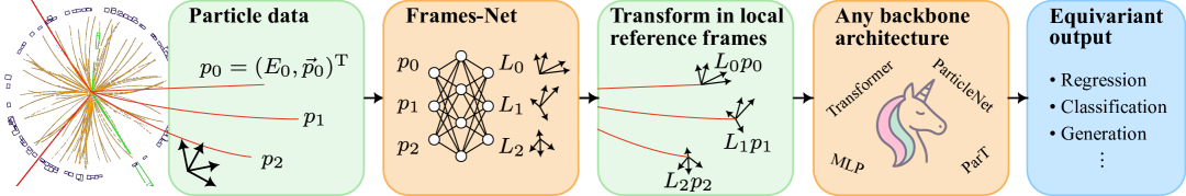
Figure 1: Lorentz Local Canonicalization (LLoCa) for making any architecture Lorentz-equivariant. The input consists of a set of particles each associated with an energy and momentum (and possibly other particle features). The particle features are transformed into learned local reference frames, turning them into Lorentz-invariant local features. The local features can then be processed by any backbone architecture to produce exactly Lorentz-equivariant outputs for a variety of possible tasks. Without including additional domain-specific priors, our approach elevates the performance of domain-agnostic models, such as a vanilla transformer, to the SOTA in the field (see e.g. Fig. 3).

In this work, we address these limitations by introducing a method that guarantees exact, but also partial and approximate, Lorentz equivariance with minimal additional computational costs. Our approach is agnostic to the architecture of the model, enabling the adaptation of existing graph neural networks (GNNs) and transformers to Lorentz-equivariant neural networks. We make the following contributions:

• To the best of our knowledge, we introduce the first (local) canonicalization framework for Lorentz-equivariant deep learning, a novel approach that does not rely on specialized layers to achieve internal representations of space-time tensors. We present a novel approach for Lorentz-equivariant prediction of local reference frames and adapt a recently proposed approach Lippmann et al. (2025) for geometric message passing to the non-compact Lorentz group. In particular, we propose a variant of scaled dot-product attention based on the Minkowski product that leverages efficient off-the-shelf attention implementations.

• Our framework is readily applicable to any non-equivariant backbone architectures. It is easy to integrate and can significantly improve the training and inference times over Lorentz-equivariant architectures that use specialized layers.

• In several experiments, we demonstrate the efficacy of exact Lorentz equivariance by achieving state-of-the-art or competitive results using a powerful Lorentz-equivariant transformer and by making several domain-specific networks Lorentz-equivariant.

• Our framework allows for a fair comparison between data augmentation and exact Lorentz equivariance. Our experiments support the superiority of Lorentz-equivariant models when ample training data is available in HEP, while data-augmentation yields the highest accuracy when training data is scarce.

• Unlike prior equivariant models, our approach incurs only a moderate computational overhead, with a 10–30% increase in FLOPs and a 30–110% increase in training time compared to non-equivariant baselines. Compared to other SOTA Lorentz-equivariant architectures, our models train up to $4\times$ faster and use $5$–$100\times$ fewer FLOPs. Upon acceptance, we will make all our code and a new dataset for QFT amplitude regression publicly available.

2 Background

Lorentz group.

The theory of special relativity Einstein (1905); Poincaré (1906) is built on two postulates: (i) the laws of physics take the same form in every inertial reference frame, and (ii) the speed of light $c$ is identical for all observers. Together they imply that every inertial observer must agree on a single scalar quantity, the spacetime interval $\Delta s^{2}=c^{2}\Delta t^{2}-\Delta\vec{x}^{2}$. Adopting natural units ($c=1$), we formalize it with the Minkowski product

$$\langle x,y\rangle=x^{0}y^{0}-x^{1}y^{1}-x^{2}y^{2}-x^{3}y^{3}\;.$$ (1)

The Minkowski product acts on column four-vectors $x=(x^{0},\vec{x})^{T}\in\mathbb{R}^{4}$, which can be decomposed into a temporal part $x^{0}$ and a spatial part $\vec{x}=(x^{1},x^{2},x^{3})^{T}$. Equation (1) can be compactly written as $x^{T}gy$ using the Minkowski metric $g=\text{diag}(1,-1,-1,-1)$ (Minkowski, 1908). Hence, frame-to-frame transformations can be represented as matrices $\Lambda\in\mathbb{R}^{4\times 4}$ that preserve the Minkowski product, i.e. that fulfill $\Lambda^{T}g\Lambda=g$. The inverse transformation is given by $\Lambda^{-1}=g\Lambda^{T}g$. Lorentz transformations $\Lambda$ act on four-vectors $x$ as $x\to x^{\prime}=\Lambda x$. The collection of all Lorentz transformations constitutes the Lorentz group $\text{O}(1,3)$. In the following we will focus on the special orthochronous Lorentz group $\text{SO}^{+}(1,3)$, which emerges as a subgroup with the constraints $\det\Lambda=1,\Lambda_{00}>0$.

A convenient parametrization of a Lorentz transformation $\Lambda\in\mathrm{SO}^{+}(1,3)$ is obtained via polar decomposition, which factors the transformation into a purely spatial rotation $R$ and a boost $B$

$$\Lambda=RB=\begin{pmatrix}1&\vec{0}^{T}\\ \vec{0}&\tilde{R}\end{pmatrix}\begin{pmatrix}\gamma&-\gamma\vec{\beta}^{T}\\ -\gamma\vec{\beta}&I_{3}+(\gamma-1)\frac{\vec{\beta}\vec{\beta}^{T}}{\vec{\beta}^{2}}\end{pmatrix},\qquad\gamma=(1-\vec{\beta}^{2})^{-1/2}.$$ (2)

In this decomposition, $R$ leaves the time component of a four-vector untouched while the submatrix $\tilde{R}\in\mathbb{R}^{3\times 3}$ rotates its spatial coordinates. Meanwhile, $B$ performs a hyperbolic “rotation” that mixes time with a chosen spatial direction determined by the dimensionless velocity vector $\vec{\beta}$. The Lorentz factor $\gamma=(1-\vec{\beta}^{2})^{-1/2}$ encodes the amount of time-dilation and length-contraction introduced by the boost. Every four-vector $p=(p^{0},\vec{p})$, with positive norm $m=(\langle p,p\rangle)^{1/2}$, defines such a boost $B(p)$ with velocity $\vec{\beta}=\vec{p}/p_{0}$.

Group representations.

To characterize how transformations of a group $G$ act on elements of a vector space $V$, we use a group representation: a map $\rho$ that assigns an invertible matrix $\rho(g)\in\mathrm{GL}(V)$ to each group element such that $\rho(g_{1}g_{2})=\rho(g_{1})\rho(g_{2})$ holds for any pair of group elements $g_{1},g_{2}\in G$. In this expression, $g_{1}g_{2}$ is the group product and $\rho(g_{1})\rho(g_{2})$ the matrix product. For instance, four-vectors transform under the 4-dimensional vector representation of the Lorentz group, $x^{\prime}=\Lambda x$, or in components, $x^{\prime\mu}=\sum_{\nu}{\Lambda^{\mu}}_{\nu}x^{\nu}$. Higher-order tensor representations follow the pattern

$$f^{\prime\mu_{1}...\mu_{n}}=\left(\rho(\Lambda)f\right)^{\mu_{1}\dots\mu_{n}}=\sum_{\nu_{1}\dots\nu_{n}}\Lambda^{\mu_{1}}_{\phantom{\mu_{1}}\nu_{1}}\ ...\ \Lambda^{\mu_{n}}_{\phantom{\mu_{n}}\nu_{n}}f^{\nu_{1}...\nu_{n}}.$$ (3)

A tensor with $n$ indices is said to have order $n$; each index runs over four spacetime directions, so the associated representation acts on a $4^{n}$-dimensional space.

Equivariance.

Geometric deep learning takes advantage of the symmetries already present in a problem instead of forcing the model to “rediscover” them from data Cohen (2021); Bronstein et al. (2021). An operation $f$ is equivariant to a symmetry group $G$ when the group action commutes with the function, i.e. $f(g\cdot x)=g\cdot f(x)$ for any $g\in G$. Invariance of $f$ emerges as a special case of equivariance if the output is invariant under group actions, $f(g\cdot x)=f(x)$.

High-energy physics.

In most steps of a HEP analysis pipeline, the data takes the form of a set of particles. Each particle is characterized by its discrete particle type as well as its energy $E$ and three-momentum $\vec{p}$ which make up the four-momentum $p=(E,\vec{p})^{T}\in\mathbb{R}^{4}$. Four-momenta transform in the vector representation of the Lorentz group. Examples for particle types are fundamental particles like electrons, photons, quarks and gluons as well as reconstructed objects like “jets“ Salam (2010). In addition to the particle mass $m=(\langle p,p\rangle)^{1/2}$, particles might be described by extra scalar information depending on the application. Particle data is typically processed with permutation-equivariant architectures such as graph networks and transformers, with each particle corresponding to one node or token in a fully connected graph.

Lorentz symmetry breaking.

Although the underlying dynamics of high-energy physics respect the full Lorentz group $\mathrm{SO}^{+}(1,3)$, the experimental environment in HEP introduces explicit symmetry breaking. The proton beams as well as the detector geometry single out a preferred spatial axis, breaking the symmetry of rotations around axes orthogonal to the beam direction. Further, reconstruction algorithms use the transverse momentum $(p_{x}^{2}+p_{y}^{2})^{1/2}$ to define jets, a quantity which is only invariant under rotations around the beam axis. As a result, many collider observables retain at most a residual $\mathrm{SO}(2)$ symmetry of rotations about the beam axis. In particular, the classification score in Sec. 5.1 is only $\mathrm{SO}(2)$-equivariant, while the regression target in Sec. 5.2 is fully Lorentz-equivariant.

Nevertheless, Lorentz-equivariant networks outperform $\mathrm{SO}(2)$-invariant networks in tasks with partial Lorentz symmetry breaking Gong et al. (2022); Bogatskiy et al. (2022); Ruhe et al. (2023); Spinner et al. (2024). This is achieved through a flexible symmetry breaking strategy that preserves Lorentz-equivariant hidden representations. Typically, fixed reference four-vectors such as the global time direction $(1,0,0,0)$ and beam axis $(0,0,0,1)$ are provided as inputs, restricting equivariance to transformations that leave these vectors invariant.

3 Related work

Lorentz-equivariant architectures.

Neural networks with exact Lorentz equivariance have emerged as a powerful tool for HEP analyses. A basic approach achieves Lorentz invariance by projecting the particle cloud onto all pairwise Minkowski inner products and processing the results with an MLP Spinner et al. (2024); Bresó et al. (2024). The lack of permutation equivariance in this design is overcome by PELICAN Bogatskiy et al. (2022), which uses layers that capture all permutation-equivariant mappings on edge features. Predicting non-scalar quantities such as four-vectors demands internal features that transform in Lorentz group representations. LorentzNet Gong et al. (2022) uses scalar and vector channels, while CGENN Ruhe et al. (2023) and L-GATr Spinner et al. (2024); Brehmer et al. (2024b) adopt geometric algebra representations, including antisymmetric second-order tensors. CGENN and LorentzNet use message passing, whereas L-GATr relies on self-attention. Unlike these models, LLoCa supports arbitrary representations with fewer architectural constraints and improved efficiency.

Equivariance by local canonicalization.

An alternative approach to achieve equivariance is to transform the input data into a canonical reference frame. An arbitrary backbone network then acts on the canonicalized input before a final transformation back to the initial reference frame provides the equivariant output. Unlike global canonicalization, local canonicalization Kaba et al. (2023) facilitates that similar local substructures will yield similar local features. Several methods have been proposed to find a global canonical orientation for 3D point cloud data (Zhao et al., 2020; Li et al., 2021; Zhao et al., 2022; Baker et al., 2024), or a local canonicalization for the compact group of 3D rotations and reflections (Wang and Zhang, 2022; Luo et al., 2022; Du et al., 2024). However, to the best of our knowledge, there exist no equivalents for the non-compact Lorentz group. As shown in Lippmann et al. (2025), properly transforming tensorial objects between reference frames during message passing substantially increases the expressivity of the architecture. We extend their solution to the Lorentz group.

Scaling of exact equivariance vs. data augmentation.

Recent work has begun to probe approximate symmetries in neural networks (Langer et al., 2024) and to question whether exact equivariance improves data scaling laws of neural networks (Brehmer et al., 2024a; Lippmann et al., 2025). Building on local canonicalization, our framework enables a controlled comparison: it allows us to evaluate an exactly Lorentz-equivariant model and an equally engineered, non-equivariant counterpart trained with data augmentation on equal footing. We conduct several experiments to investigate how both types of models scale with the amount of training data.

4 Methods

The general idea of our framework is the following (cf. Fig. 1): for every particle, or node, we predict a local reference frame which transforms equivariantly under general Lorentz transformations. Then, we express the particle features in the predicted local reference frames, therefore transforming them into Lorentz-invariant features which can be processed by any backbone network. We obtain a Lorentz-equivariant prediction by transforming the space-time objects back to the global reference frame. In its minimal version, only local scalar information is exchanged between nodes, a constraint that significantly limits the expressivity of the architecture. We instead propose to group particle features into tensor representations and consistently construct tensorial space-time messages, extending the method proposed by Lippmann, Gerhartz et al. Lippmann et al. (2025).

4.1 Local reference frames

A local reference frame $L$ is constructed from a set of four four-vectors $u_{0},u_{1},u_{2},u_{3}$ (“vierbein”) that form an orthonormal basis in Minkowski space, i.e. they satisfy the condition

$$\sum_{\mu,\nu}{u_{a}}^{\mu}{u_{b}}^{\nu}g_{\mu\nu}=g_{ab}\;.$$ (4)

The transformation behavior of four-vectors $u_{i}\to\Lambda u_{i}$ implies that the local reference frames $L$ transform as $L\to L\Lambda^{-1}$ if constructed from row vectors in the following way

$$L=\begin{pmatrix}\rule[2.15277pt]{14.22636pt}{0.55pt}\ {u_{0}^{T}g}\ \rule[2.15277pt]{14.22636pt}{0.55pt}\\ \rule[2.15277pt]{14.22636pt}{0.55pt}\ {u_{1}^{T}g}\ \rule[2.15277pt]{14.22636pt}{0.55pt}\\ \rule[2.15277pt]{14.22636pt}{0.55pt}\ {u_{2}^{T}g}\ \rule[2.15277pt]{14.22636pt}{0.55pt}\\ \rule[2.15277pt]{14.22636pt}{0.55pt}\ {u_{3}^{T}g}\ \rule[2.15277pt]{14.22636pt}{0.55pt}\\ \end{pmatrix}\quad\overset{\Lambda}{\to}\quad L^{\prime}=\begin{pmatrix}\rule[2.15277pt]{14.22636pt}{0.55pt}\ u_{0}^{T}\Lambda^{T}g\ \rule[2.15277pt]{14.22636pt}{0.55pt}\\ \rule[2.15277pt]{14.22636pt}{0.55pt}\ u_{1}^{T}\Lambda^{T}g\ \rule[2.15277pt]{14.22636pt}{0.55pt}\\ \rule[2.15277pt]{14.22636pt}{0.55pt}\ u_{2}^{T}\Lambda^{T}g\ \rule[2.15277pt]{14.22636pt}{0.55pt}\\ \rule[2.15277pt]{14.22636pt}{0.55pt}\ u_{3}^{T}\Lambda^{T}g\ \rule[2.15277pt]{14.22636pt}{0.55pt}\\ \end{pmatrix}=L\Lambda^{-1}.$$ (5)

In the final step, we insert two Minkowski metrics as $I_{4}=gg$, allowing us to identify the inverse transformation $\Lambda^{-1}=g\Lambda^{T}g$. With this relation, the orthonormality condition (4) becomes $LgL^{T}=g$, the defining property of Lorentz transformations. In Sec. 4.5, we explicitly construct local reference frames $L$ that satisfy both conditions introduced above. When working with sets of particles, a separate local reference frame can be assigned to each particle, see Fig. 1.

4.2 Local canonicalization

Local four-vectors $x_{L}=Lx$ are defined by transforming global four-vectors $x$ into the local reference frame $L$. Thanks to the transformation rule $L\to L\Lambda^{-1}$, these local vectors remain invariant under global Lorentz transformations $\Lambda$, i.e. $x_{L}=Lx\to x^{\prime}_{L}=L\Lambda^{-1}\Lambda x=Lx=x_{L}$. This property readily generalizes to general Lorentz tensors $f$, which transform as $f\to f^{\prime}=\rho(\Lambda)f$. For features in the local reference frame $f_{L}=\rho(L)f$ we find

$$f_{L}\overset{\Lambda}{\to}f^{\prime}_{L}=\rho(L^{\prime})f^{\prime}=\rho(L\Lambda^{-1})\rho(\Lambda)f=\rho(L\Lambda^{-1}\Lambda)f=\rho(L)f=f_{L}.$$ (6)

The local particle features $f_{L}$ can be processed with any backbone architecture without violating their Lorentz invariance, cf. Fig. 1. Finally, output features $y$ in the global reference frame are extracted using the inverse transformation $y=\rho(L^{-1})f_{L}$. These output features $y$ are equivariant under Lorentz transformations

$$y\overset{\Lambda}{\to}y^{\prime}=\rho(L^{\prime-1})f^{\prime}_{L}=\rho(\Lambda L^{-1})f_{L}=\rho(\Lambda)\rho(L^{-1})f_{L}=\rho(\Lambda)y.$$ (7)

4.3 Tensorial messages between local reference frames

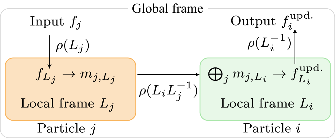
Figure 2: Tensorial message passing in LLoCa. Lorentz-invariant local messages are transformed between local reference frames.

Consider a system of $N$ particles, where a message is sent from particle $j$ to particle $i$. The message $m_{j,L_{j}}$ in the local reference frame $L_{j}$ is Lorentz-invariant, as it is constructed from the invariant particle features $f_{L_{j}}$. To communicate this message to particle $i$ in reference frame $L_{i}$, we apply the reference frame transformation matrix $L_{i}L_{j}^{-1}$, which gives the transformed message:

$$m_{j,L_{i}}=\rho(L_{i}L_{j}^{-1})m_{j,L_{j}}.$$ (8)

The message representation $\rho$ is a hyperparameter that can be chosen according to the problem. Our implementation supports general tensor representations following Eq. (3), though in practice, we find an equal mix of scalar and vector representations sufficient for our applications. Regardless of the chosen representation, the received message $m_{j,L_{i}}$ remains invariant since the transformation matrix $L_{i}L_{j}^{-1}$ is invariant:

$$L_{i}L_{j}^{-1}\overset{\Lambda}{\to}L^{\prime}_{i}L^{\prime-1}_{j}=L_{i}\Lambda^{-1}(L_{j}\Lambda^{-1})^{-1}=L_{i}\Lambda^{-1}\Lambda L_{j}^{-1}=L_{i}L_{j}^{-1}.$$ (9)

This formalism can be easily integrated into any message passing paradigm. Writing $\phi$ and $\psi$ for unconstrained neural networks and $\bigoplus$ for a permutation-invariant aggregation operation, the updated features for particle $i$ can be written as:

$$f^{\text{updated}}_{L_{i}}=\psi\bigg{(}f_{L_{i}},\bigoplus_{j=1}^{N}\phi\big{(}\rho(L_{i}\ L_{j}^{-1})\ m_{j,L_{j}}\big{)}\bigg{)}.$$ (10)

We extend this framework proposed by Lippmann, Gerhartz et al. Lippmann et al. (2025) to the Lorentz group, see Fig. 2.

Tensorial scaled dot-product attention.

A particularly prominent example of message passing is scaled dot-product attention Vaswani et al. (2017). We obtain scaled dot-product attention with tensorial message passing as a special case of Eq. (10)

$$f^{\text{updated}}_{L_{i}}=\sum_{j=1}^{N}\operatorname{softmax}\left(\frac{1}{\sqrt{d}}\Big{\langle}\ q_{L_{i}},\rho(L_{i}L_{j}^{-1})k_{L_{j}}\Big{\rangle}\right)\ \rho(L_{i}L_{j}^{-1})\ v_{L_{j}}.$$ (11)

The objects $q_{L_{j}},k_{L_{i}},v_{L_{j}}$ are the $d$-dimensional queries, keys and values, each expressed and computed in the respective local reference frame starting from the respective local node features $f_{L_{i}},f_{L_{j}}$. The softmax normalizes the attention weights over all sending nodes. The Minkowski product $\langle\cdot,\cdot\rangle$ reduces to the Euclidean product if the queries, keys and values are assigned to scalar representations $\rho$. For higher-order representations, we find that Minkowski attention outperforms Euclidean attention, see App. D. Since the Minkowski product is Lorentz-invariant,

$$\langle q_{L_{i}},\rho(L_{i}L_{j}^{-1})k_{L_{j}}\rangle=\langle\rho(L_{i}^{-1})q_{L_{i}},\rho(L_{i}^{-1})\rho(L_{i}L_{j}^{-1})k_{L_{j}}\rangle=\langle\rho(L_{i}^{-1})q_{L_{i}},\rho(L_{j}^{-1})k_{L_{j}}\rangle.$$ (12)

That is, keys and queries can simply be transformed into the global frame of reference, in which all Minkowski products can be efficiently evaluated. This facilitates the use of highly optimized scaled dot-product attention implementations Dao et al. (2022).

4.4 Relation to data augmentation

Architectures with local canonicalization achieve Lorentz equivariance if the local reference frames satisfy Eq. (5), imposing strong constraints on their construction. Non-equivariant networks emerge as a special case where the local reference frames are the identity, $L=1$. Data augmentation also emerges as a special case, where one global reference frame is drawn from a given distribution of Lorentz transformations. Implementing non-equivariant networks and data augmentation as special cases of equivariant networks enables a fair comparison between these three choices.

4.5 Constructing local reference frames

We now describe how to construct local reference frames for a set of particles, the typical data type in high-energy physics. Local reference frames $L$ have to satisfy the Lorentz group condition $L^{T}gL=g$ and transform as $L\to L^{\prime}=L\Lambda^{-1}$ under Lorentz transformations $\Lambda$. The local reference frames are constructed in two steps: first we use a simple Lorentz-equivariant architecture to predict three four-vectors for each particle. The four-vectors are then used to construct the local reference frames $L$ following a deterministic algorithm.

In a system of $N$ particles, each particle is described by its four-momentum $p_{i}$ and additional scalar attributes $s_{i}$, such as the particle type. For each particle $i$, the three four-vectors are predicted as

$$v_{i,k}=\sum_{j=1}^{N}\operatorname{softmax}\Big{(}\varphi_{k}(s_{i},s_{j},\langle p_{i},p_{j}\rangle)\Big{)}(p_{i}+p_{j})\quad\text{ for }k=0,1,2.$$ (13)

Algorithm 1 Local reference frames via polar decomposition

1:$v_{0},v_{1},v_{2}\in\mathbb{R}^{4}$ with $v^{\prime}_{i}=\Lambda v_{i}$, $\langle v_{0},v_{0}\rangle>0$

2:$L^{T}gL=g$ and $L\to L^{\prime}=L\Lambda^{-1}$

3:$B\leftarrow B(v_{0})$ using Eq. (2)

4:$w_{k}\leftarrow Bv_{k}$ for $k=1,2$

5:$\vec{u}_{1},\vec{u}_{2},\vec{u}_{3}\leftarrow\operatorname{GramSchmidt}(\vec{w}_{1},\vec{w}_{2})$

6:$\tilde{R}\leftarrow(\vec{u}_{1},\vec{u}_{2},\vec{u}_{3})^{T}$

7:$R\leftarrow\begin{pmatrix}1&\vec{0}^{T}\\ \vec{0}&\tilde{R}\\ \end{pmatrix}$

8:$L\leftarrow RB$

This operation is Lorentz-equivariant because it constructs four-vectors as a linear combination of four-vectors with scalar coefficients Villar et al. (2021). The function $\varphi$ is an MLP operating on Lorentz scalars with three output channels. Empirically, we find that a network $\varphi$ that is significantly smaller than the backbone network is already sufficient, see App. C. To ensure positive and normalized weights, a softmax is applied across the weights of all sending nodes. This constrains the resulting vectors $v_{i,k}$ to have positive inner products $\langle v_{i,k},v_{i,k}\rangle>0$, given that the input particles have positive inner products and positive energy $p_{i}^{0}>0$. We observe that the softmax operation significantly improves numerical stability during the subsequent orthonormalization procedure. Indeed, large boosts $B$ may lead to numerical instabilities. However, although the particles $p_{i}$ are highly boosted, we find that the predicted vectors $v_{i,k}$ typically are not, resulting in stable training. In tasks where symmetry breaking effects reduce full Lorentz symmetry to a subgroup, we incorporate reference particles (cf. Sec. 2) which are needed only for the local frame prediction.

For each particle $i$, the local reference frame $L_{i}$ is constructed from the three four-vectors $v_{i,k},k=0,1,2$ using polar decomposition, cf. Eq. (2). For readability, we omit the particle index $i$ from here on. As outlined in Alg. 1, the boost $B(v_{0})$ is built from $v_{0}$, while the rotation $R$ is derived from $v_{1}$ and $v_{2}$. These two vectors are first transformed with the same boost and then orthonormalized via the Gram-Schmidt algorithm. Linear independence of $v_{1}$ and $v_{2}$ is required, but we find this holds reliably for systems with $N\geq 3$ particles. Alg. 1 is equivalent to a Gram-Schmidt algorithm in Minkowski space; see App. B for details and a proof that $L$ satisfies the transformation rule $L\to L\Lambda^{-1}$. The above construction contains equivariantly predicted rotations for $\mathrm{SO}(3)$-equivariant architectures as a special case with $v_{0}=(1,0,0,0)$, though this restricted variant yields inferior performance, see App. D.

5 Experiments

We now demonstrate the effectiveness of Lorentz Local Canonicalization (LLoCa) for a range of different architectures on two relevant tasks in HEP. We start from the classification of jets, or “jet tagging”. Then, we present extensive studies on the QFT amplitudes regression.

5.1 Jet tagging

Jet tagging is the identification of the mother particle which initiated the spray of hadrons, a “jet”, from a set of reconstructed particles. This task plays a key role in HEP workflows, where even marginal gains in classification performance lead to purer datasets and reduced data-taking time – ultimately saving experimental resources. For this application the big-data regime is most interesting, because simulating training data is cheap. Therefore, we use the JetClass dataset Qu et al. (2024), a modern benchmark dataset that contains 125M jets divided into 10 classes.

The ParticleNet Qu and Gouskos (2020) and ParT Qu et al. (2024) networks are established jet tagging architectures in the high-energy physics community. ParticleNet uses dynamic graph convolutions, and ParT is a transformer with class attention Touvron et al. (2021) and a learnable attention bias based on Lorentz-invariant edge attributes. We use the LLoCa framework to make both architectures Lorentz-equivariant with minimal adaptations to the official implementation, see Tab. 1. Further, we compare against a vanilla transformer and its LLoCa adaptation (cf. Sec. 4.3), see App. C for details.

Without any hyperparameter tuning, the Lorentz-equivariant models based on LLoCa consistently outperform their non-equivariant counterparts, at the cost of some extra training time and FLOPs (see Tab. 1). Interestingly, LLoCA can elevate the performance of the domain-agnostic transformer to the performance of the domain-specific ParT architecture. This indicates that LLoCa provides an effective inductive bias, without the need for specialized architectural designs.

Table 1: LLoCa consistently improves the performance of non-equivariant architectures. For classification on the JetClass dataset we compare accuracy, area under the ROC curve (AUC) as well as training time on a H100 GPU and FLOPs for a forward pass with batch size 1 for the JetClass dataset from Qu et al. (2024). For our models, accuracy and AUC metrics are significant up to the last digit. LLoCa improves domain-specific architectures and elevates a vanilla transformer to competitive accuracy (* indicates Lorentz equivariance). For more metrics, see Tab. 5.

Model	Accuracy ($\uparrow$)	AUC ($\uparrow$)	Time	FLOPs
PFN (Komiske et al., 2019)	0.7720	0.97140	$3$h	$3$M
P-CNN (Sirunyan et al., 2020)	0.8090	0.97890	$3$h	$12$M
MIParT (Wu et al., 2025)	0.8610	0.98780	–	–
L-GATr* (Brehmer et al., 2024b)	0.8660	0.98850	$180$h	$2060$M
ParticleNet (Qu and Gouskos, 2020)	0.8440	0.98490	$27$h	$413$M
LLoCa-ParticleNet*	0.845	0.9852	$41$h	$517$M
ParT (Qu et al., 2024)	0.8610	0.98770	$38$h	$211$M
LLoCa-ParT*	0.864	0.9882	$67$h	$315$M
Transformer	0.855	0.9867	$17$h	$210$M
LLoCa-Transformer*	0.864	0.9882	$33$h	$301$M

5.2 QFT amplitude regression

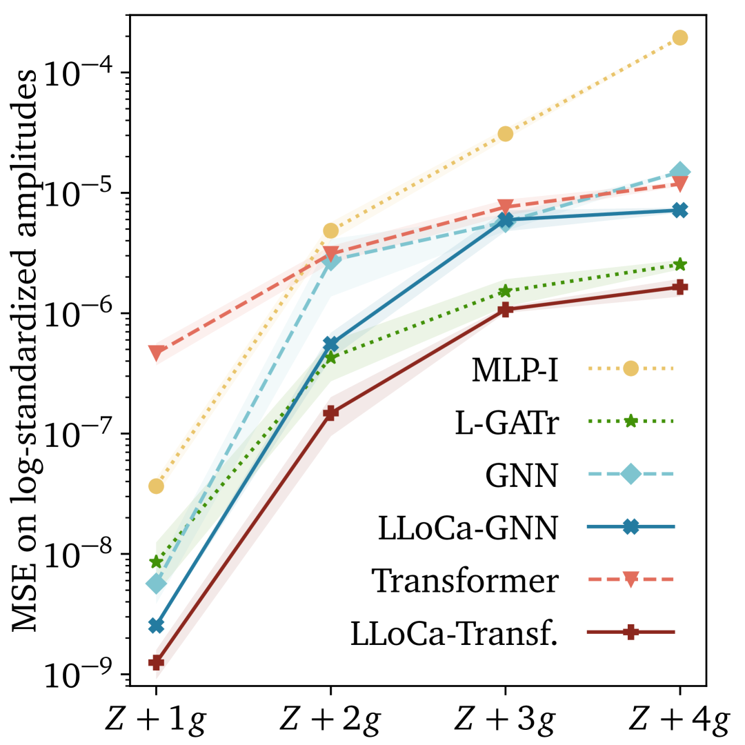
Model	MSE$\times 10^{-6}$ ($\downarrow$)		FLOPs	Time
MLP-I Spinner et al. (2024)	$195.0$ $\pm$	2	$0.1$M	$0.6$h
LGATr Spinner et al. (2024)	$2.5$ $\pm$	0.2	$1160.0$M	$19.5$h
GNN	$14.9$ $\pm$	0.3	$9.9$M	$1.3$h
LLoCa-GNN	7.2 $\pm$	0.3	$10.6$M	$2.3$h
Transformer	$11.9$ $\pm$	0.5	$10.6$M	$3.5$h
LLoCa-Transformer	00 1.5 $\pm$	0.1	$11.3$M	$4.5$h

Figure 3: LLoCa surpasses SOTA performance while being $\boldsymbol{4\times}$ faster. The collisions of two particles produces a single $Z$ boson and $n=1,2,3,4$ many gluons $g$ (x-ticks $Z+ng$). LLoCa significantly improves the prediction of interaction amplitudes of the non-equivariant GNN and transformer. Left: Our LLoCa-Transformer achieves state-of-the-art results over all four multiplicities. Right: Accuracy and compute for $Z+4g$. The LLoCa-Transformer uses a tenth of the FLOPs and a quarter of the training time relative to the second most accurate model. Uncertainties are standard deviations over three runs. See App. C for more details.

In collisions of fundamental particles, the occurrence of a specific final state is governed by a probability. This probability is a function of the four-momenta of the incoming and outgoing particles, as well as their particle types. Using the framework of Quantum Field Theory (QFT), we can calculate this probability or “amplitude” in a perturbative expansion. Neural surrogates Badger and Bullock (2020); Maˆıtre and Truong (2021); Aylett-Bullock et al. (2021); Maˆıtre and Truong (2023); Badger et al. (2023); Bresó et al. (2024); Spinner et al. (2024) can greatly speed up this process, since the factorial growth of possible interactions with increasing particle number often makes exact evaluation unfeasible. The exact Lorentz invariance of amplitudes makes them a prime candidate for a LLoCa surrogate model.

We follow Spinner et al. (2024) and benchmark our Lorentz Local Canonicalization (LLoCa) approach on the process $q\bar{q}\to Z+ng$, the production of a $Z$ boson with $n=1,\dots,4$ additional gluons from a quark-antiquark pair. The surrogates are trained for each value of $n$ separately. We evaluate the neural surrogates in terms of the standardized Mean Squared Error (MSE) between the predictions and ground truth amplitudes. Architectures and training details are described in App. C.

LLoCa allows us to upgrade any non-equivariant baselines and directly study the benefits of built-in Lorentz equivariance. To that end, we construct LLoCa adaptations of a baseline graph neural network (GNN) and a vanilla transformer as described in Sec. 4.3. For comparison, we consider a simple MLP acting on Lorentz-invariants (MLP-I) Bresó et al. (2024) and the performant L-GATr Spinner et al. (2024). LLoCa consistently improves the accuracy of non-equivariant architectures, see Fig. 3. Crucially, without including additional domain-specific priors, our LLoCa-Transformer achieves state-of-the-art-performance, outperforming the significantly more expensive L-GATr architecture over the entire range of multiplicities.

Message representations.

Table 2: Effectiveness of tensorial messages. LLoCa-Transformer with different hidden tensor representations on $Z+4g$ QFT amplitude regression.

Method	MSE ($\times 10^{-6}$)
Non-equivariant	$11.9$ $\pm$	0.8
Global canonical.	$5.9$ $\pm$	0.4
LLoCa ($16$ scalars)	$54.0$ $\pm$	3
LLoCa (single 2-tensor)	$2.4$ $\pm$	0.3
LLoCa ($4$ vectors)	$2.0$ $\pm$	0.2
LLoCa ($8$ scalars, $2$ vectors)	$1.5$ $\pm$	0.1

Beyond the improvements obtained through exact Lorentz equivariance, we have identified the tensorial message passing in LLoCa (cf. Sec. 4.3) as a crucial factor for expressive message passing based on local canonicalization. We compare the performance of the LLoCa-transformer with different message representations in the 16-dimensional attention head, see Tab. 2. We compare 16 scalars against four 4-dimensional vectors, a single 16-dimensional second-order tensor representations as well as our default of eight scalars combined with two four-vectors. All tensorial representations significantly outperform the scalar message passing. For reference, we include the non-equivariant transformer and the same model with global canonicalization (one shared learned reference frame to every particle).

Lorentz equivariance at scale.

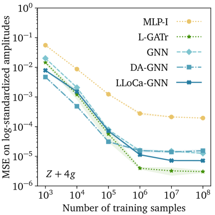
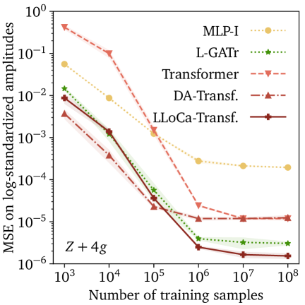
Figure 4: Data efficiency of LLoCa networks. Lorentz-equivariant amplitude regression for $Z+4g$ production is more data efficient in the large data regime for both graph networks (left) and transformers (right). Perhaps surprisingly, data augmentation (DA) outperforms equivariance for small datasets.

Lorentz equivariance introduces a strong inductive bias in neural networks, typically at the cost of extra compute. Data augmentation provides a cheap alternative which aims at learning approximate Lorentz equivariance directly from data. LLoCa includes data augmentation as a special case, allowing us to directly compare exact Lorentz equivariance (LLoCa) with data augmentation (DA) using the same backbone architecture and training parameters. For this purpose, we focus on the most complicated process $Z+4g$ and train surrogate models with different fractions of the training dataset, see Fig. 4. Augmented trainings outperform the non-equivariant baseline for small training datasets due to the symmetry group information encoded in data augmentations, but the two approaches agree for large dataset sizes where model expressivity becomes the limiting factor. The Lorentz-equivariant models surpass the competition in this big-data regime due to their increased expressivity at fixed parameter count. Interestingly, we observe that trainings with data augmentation outperform even the Lorentz-equivariant models for small training dataset sizes. We include extensive ablation studies on the method used for local canonicalization, tensorial message representations, and data augmentation in App. D.

5.3 Computational efficiency

While Lorentz-equivariant architectures offer valuable inductive biases, they often come with significant computational overhead compared to the corresponding non-equivariant architectures. To evaluate this trade-off, we report both nominal FLOPs – which capture architectural complexity – and empirical training time, which also reflects implementation efficiency, in Tab. 1 and Fig. 3. Our LLoCa models introduce a modest increase in computational cost, with FLOPs rising by 10–30% and training time by 30–110%, depending on the task and architecture. In contrast, the state-of-the-art L-GATr architecture Spinner et al. (2024) incurs significantly higher costs, with a $5$–$100\times$ increase in FLOPs and a $4\times$ increase in training time relative to our LLoCa-Transformer.

6 Conclusion

Particle physics provides ample data and studies systems that exhibit Lorentz symmetry. Neural networks that respect Lorentz symmetry have emerged as essential tools in accurately analyzing the data and modeling the underlying physics. However, existing Lorentz-equivariant architectures introduce large computational costs and rely on specialized building blocks, which limits the architectural design space and hinders the transfer of deep learning progress from other modalities. We address these issues by introducing Lorentz Local Canonicalization (LLoCa), a novel framework that can make any off-the-shelf architecture Lorentz-equivariant. In several experiments, we have demonstrated the effectiveness of LLoCa by achieving state-of-the-art results even with domain-agnostic backbone architectures. Furthermore, our approach significantly improves established domain-specific but non-equivariant architectures, without any hyperparameter tuning. While the LLoCa framework introduces a computational overhead, our LLoCa models are still significantly faster at training and inference than other SOTA Lorentz-equivariant networks. We hope that LLoCa facilitates the design of novel Lorentz-equivariant architectures and helps to bridge innovations between machine learning in particle physics and other domains.

Acknowledgements

The authors thank Víctor Bresó for generating the amplitude regression datasets. They are also grateful to Huilin Qu for assistance with the JetClass dataset and for support with the ParticleNet and ParT implementations. Further thanks go to Johann Brehmer, Víctor Bresó, Jesse Thaler, and Henning Bahl for valuable discussions and insightful feedback on the manuscript.

The authors acknowledge support by the state of Baden-Württemberg through bwHPC and the German Research Foundation (DFG) through the grants INST 35/1597-1 FUGG and INST 39/1232-1 FUGG. Computational resources have been provided by the supercomputing facilities of the Université catholique de Louvain (CISM/UCL) and the Consortium des Équipements de Calcul Intensif en Fédération Wallonie Bruxelles (CÉCI) funded by the Fond de la Recherche Scientifique de Belgique (F.R.S.-FNRS) under convention 2.5020.11 and by the Walloon Region. The present research benefited from computational resources made available on Lucia, the Tier-1 supercomputer of the Walloon Region, infrastructure funded by the Walloon Region under the grant agreement n°1910247.

J.S. and T.P. are supported by the Baden-Württemberg-Stiftung through the program Internationale Spitzenforschung, project Uncertainties — Teaching AI its Limits (BWST_IF2020-010), the Deutsche Forschungsgemeinschaft (DFG, German Research Foundation) under grant 396021762 – TRR 257 Particle Physics Phenomenology after the Higgs Discovery. J.S. is funded by the Carl-Zeiss-Stiftung through the project Model-Based AI: Physical Models and Deep Learning for Imaging and Cancer Treatment. L.F. is supported by the Fonds de la Recherche Scientifique - FNRS under Grant No. 4.4503.16. P.L. and F.A.H. acknowledge funding by Deutsche Forschungsgemeinschft (DFG, German Research Foundation) – Projektnummer 240245660 - SFB 1129.

This work is supported by Deutsche Forschungsgemeinschaft (DFG) under Germany’s Excellence Strategy EXC-2181/1 - 390900948 (the Heidelberg STRUCTURES Excellence Cluster).

Appendix A Tensor representation

The tensor representation is introduced in Eq. 3. The tensor representation is a group representation of the Lorentz group $\mathrm{O}(1,3)$ and is used in this paper to define the transformation behavior of tensorial space-time features when transformed in or out of local reference frames.

Proof representation property.

The representation property follows from the fact that the $4\times 4$ Lorentz transform matrices itself form a representation. For any $\Lambda_{1},\Lambda_{2}\in\mathrm{SO}^{+}(1,3)$ we have

$$[\rho(\Lambda_{1})\rho(\Lambda_{2})T]^{\mu_{1}...\mu_{n}} ={{\Lambda_{1}}^{\mu_{1}}}_{\rho_{1}}\ ...\ {{\Lambda_{1}}^{\mu_{n}}}_{\rho_{n}}{{\Lambda_{2}}^{\rho_{1}}}_{\nu_{1}}\ ...\ {{\Lambda_{2}}^{\rho_{n}}}_{\nu_{n}}T^{\nu_{1}...\nu_{n}}$$

$$={(\Lambda_{1}\Lambda_{2})^{\mu_{1}}}_{\nu_{1}}\ ...\ {(\Lambda_{1}\Lambda_{2})^{\mu_{n}}}_{\nu_{n}}=[\rho(\Lambda_{1}\Lambda_{2})T]^{\mu_{1}...\mu_{n}}$$ (14)

Representation hidden features.

The input and output representations are determined by the input data and the prediction task. Contrarily, the internal representations are chosen as hyperparameters. In our framework, we choose a direct sum of tensor representations, which again forms a representation. A feature $f$ will transform under $\rho_{\mathrm{f}}=\rho_{1}\oplus...\oplus\rho_{k}$ with a block diagonal matrix:

$$\rho_{\mathrm{f}}(\Lambda)f=\begin{pmatrix}\rho_{1}(\Lambda)\\ &\ddots\\ &&\rho_{k}(\Lambda)\end{pmatrix}f$$ (15)

So that the composition of scalar, vectorial and tensorial features can be chosen freely. The feature dimension of $f$ will be given by $\dim(f)=\dim(\rho_{1})+...+\dim(\rho_{k})$.

Appendix B Background information on the construction of local reference frames

B.1 Gram-Schmidt algorithm in Minkowski space

In this section we discuss how to construct reference frames $L$ that satisfy the transformation behaviour $L\to L\Lambda^{-1}$ of Eq. (5) directly with a Gram-Schmidt orthonormalization algorithm adapted for Minkowski vectors. Similar to Alg. 1, this algorithm starts from three Lorentz vectors $v_{0},v_{1},v_{2}$ and returns a local reference frame $L$. The difference to Alg. 1 is that there $L$ is decomposed into a rotation and a boost, whereas here we construct $L$ directly from a set of four orthonormal vectors, as illustrated in Eq. (5).

We identified two advantages to the polar decomposition approach (PD) described in Alg. 1 compared to the Gram-Schmidt algorithm in Minkowski space ($\mathrm{GS}^{4}$) described above. First, the PD has the conceptional advantage of explicitly seperating the boost and rotation. This allows to easily study properties of the boost and rotation parts independently, identify the special cases of a pure boost and a pure rotation, and for example constrain the magnitude of the boost vector $v_{0}$. Second, we find that the PD approach of boosting into a reference frame typical for the particle set and then orthonormalising two vectors in that frame is numerically more stable than the $\mathrm{GS}^{4}$ approach of directly orthonormalising a set of three vectors. Throughout our experiments, we find that the PD and $\mathrm{GS}^{4}$ approaches yield similar performance, see App. D, with the tendency of PD being slightly better in all our experiments.

Starting from three Lorentz vectors $v_{0},v_{1},v_{2}$, we apply the following algorithm to obtain four four-vectors $u_{0},u_{1},u_{2},u_{3}$ that satisfy Eq. (4)

$$\operatorname{norm}(v) =\frac{v}{\|v\|+\epsilon},$$

$$a_{i} =\operatorname{norm}(v_{i})\quad\text{for}\quad i=0,1,2,$$

$$u_{0} =a_{0},$$

$$u_{1} =\operatorname{norm}\left(a_{1}-u_{0}\frac{\langle a_{1},u_{0}\rangle}{\langle u_{0},u_{0}\rangle}\right),$$

$$u_{2} =\operatorname{norm}\left(a_{2}-u_{0}\frac{\langle a_{2},u_{0}\rangle}{\langle u_{0},u_{0}\rangle}-u_{1}\frac{\langle a_{2},u_{1}\rangle}{\langle u_{1},u_{1}\rangle}\right),$$

$$u_{3}^{\mu} =\sum_{\nu,\rho,\sigma,\kappa}g^{\mu\nu}\epsilon_{\nu\rho\sigma\kappa}u_{0}^{\rho}u_{1}^{\sigma}u_{2}^{\kappa}.$$ (16)

We use $\epsilon=10^{-15}$ and the absolute value of the Lorentz inner product $\|x\|=\sqrt{|\langle x,x\rangle|}$. The last line uses the Minkowski index notation to construct $u_{3}$ using the totally antisymmetric tensor $\epsilon_{\mu\nu\rho\sigma}$, the extension of the cross product to Minkowski space. This tensor is defined as $\epsilon_{0123}=1$, and it flips sign under permutation of any pair of indices.

When constructing the local reference frames $L$ from this orthonormal set of vectors $u_{0},u_{1},u_{2},u_{3}$, it is important to additionally transform them into covectors $u_{k}^{T}g$, where $u_{k}$ denote the vectors constructed in the algorithm above.

B.2 Proof that polar decomposition via Alg. 1 is equivalent to a Gram-Schmidt algorithm in Minkowski space

Let us first consider the Gram-Schmidt algorithm in Minkowski space (denoted by $\mathrm{GS}^{4}$). As for Alg. 1 we start from the set of four-vectors $v_{k},k=0,1,2$ as predicted by Eq. (13), assuming $\langle v_{0},v_{0}\rangle>0$. Now, we use the Gram-Schmidt algorithm in Minkowski space described in Eq. (B.1), to orthonormalize the three vectors: $\{u_{k}\}_{k=0,1,2,3}=\mathrm{GS}^{4}(v_{0},v_{1},v_{2})$. Then, the transformation matrix constructed from these orthonormal vectors is

$$L^{\mathrm{GS}}=\begin{pmatrix}\rule[2.15277pt]{14.22636pt}{0.55pt}\ {u_{0}^{T}g}\ \rule[2.15277pt]{14.22636pt}{0.55pt}\\ \rule[2.15277pt]{14.22636pt}{0.55pt}\ {u_{1}^{T}g}\ \rule[2.15277pt]{14.22636pt}{0.55pt}\\ \rule[2.15277pt]{14.22636pt}{0.55pt}\ {u_{2}^{T}g}\ \rule[2.15277pt]{14.22636pt}{0.55pt}\\ \rule[2.15277pt]{14.22636pt}{0.55pt}\ {u_{3}^{T}g}\ \rule[2.15277pt]{14.22636pt}{0.55pt}\end{pmatrix}$$ (17)

Eq. 17 has the correct transformation behavior $L\to L\Lambda^{-1}$ as shown in Eq. (5) since $\{u_{k}\}_{k=0,1,2,3}$ are also four-vectors due to the Lorentz-equivariance of $\mathrm{GS}^{4}$. According to the polar decomposition, we can decompose a proper Lorentz transformation into a pure rotation $R$ and a general boost $B$. By realizing that

$$L=RB=\begin{pmatrix}1&0\\ 0&\tilde{R}\end{pmatrix}\begin{pmatrix}\gamma&-\gamma\vec{\beta}^{\mathrm{T}}\\ -\gamma\vec{\beta}&...\end{pmatrix}=\begin{pmatrix}\gamma&-\gamma\vec{\beta}^{\mathrm{T}}\\ ...&...\end{pmatrix},$$ (18)

we can identify the boost part of a Lorentz transformation from the first row, i.e. if we consider $L^{\mathrm{GS}}=R^{\mathrm{GS}}B^{\mathrm{GS}}$

$$B^{\mathrm{GS}}=B(\vec{\beta}=-\vec{u}_{0}/u_{0}^{0})=:B(u_{0}).$$ (19)

Also note that $u_{0}=v_{0}/\langle v_{0},v_{0}\rangle$ due to the design of $\mathrm{GS}^{4}$, therefore $B(u_{0})=B(v_{0})$. Consequently, the pure rotation $R^{\mathrm{GS}}$ is given by

$$R^{\mathrm{GS}}=L^{\mathrm{GS}}{(B^{\mathrm{GS}})}^{-1}=\begin{pmatrix}\rule[2.15277pt]{14.22636pt}{0.55pt}\ {u_{0}^{T}gB(v_{0})^{-1}}\ \rule[2.15277pt]{14.22636pt}{0.55pt}\\ \rule[2.15277pt]{14.22636pt}{0.55pt}\ {u_{1}^{T}gB(v_{0})^{-1}}\ \rule[2.15277pt]{14.22636pt}{0.55pt}\\ \rule[2.15277pt]{14.22636pt}{0.55pt}\ {u_{2}^{T}gB(v_{0})^{-1}}\ \rule[2.15277pt]{14.22636pt}{0.55pt}\\ \rule[2.15277pt]{14.22636pt}{0.55pt}\ {u_{3}^{T}gB(v_{0})^{-1}}\ \rule[2.15277pt]{14.22636pt}{0.55pt}\end{pmatrix}.$$ (20)

We now show that the local frame from the polar decomposition (PD) presented in Alg. 1, $L^{\mathrm{PD}}$, is equivalent to $L^{\mathrm{GS}}$. Starting from the same set of four-vectors $v_{k},k=0,1,2$, we first construct the rest frame boost of $B(v_{0})$. Since $B(u_{0})=B(v_{0})$, the boosts in polar decomposition and Minkowski Gram-Schmidt are equal, $B^{\mathrm{PD}}=B^{\mathrm{GS}}$. To prove that the rotation parts agree as well, $R^{\mathrm{PD}}=R^{\mathrm{GS}}$, we first show that $\{(0,\mathrm{GS}^{3}(B(v_{0})v_{1},B(v_{0})v_{2}))_{k}\}_{k=0,1,2}=\{\mathrm{GS}^{4}(B(v_{0})v_{0},B(v_{0})v_{1},B(v_{0})v_{2})_{k}\}_{k=1,2,3}$. Indeed,

$$u_{0}=\mathrm{norm}(B(v_{0})v_{0})=(1,\vec{0})\;,$$

$$\langle a_{1},u_{0}\rangle=(a_{1}^{0}u_{0}^{0},\vec{0})\;,\qquad u_{1}^{0}=\mathrm{norm}(a_{1}^{0}(1-u_{0}^{0}{{}^{2}}))=0\;,$$ (21)

and similarly for the other vectors $u_{2},u_{3}$. Therefore, the first component of the $\mathrm{GS}^{4}$ vectors different from $v_{0}$ is always zero while the spatial components are equal to those obtain from $\mathrm{GS}^{3}$. Since $\mathrm{GS}^{4}$ is Lorentz-equivariant, we have $\mathrm{GS}^{4}(B(v_{0})v_{0},B(v_{0})v_{1},B(v_{0})v_{2})=B(v_{0})\mathrm{GS}^{4}(v_{0},v_{1},v_{2})=B(v_{0})\{u_{k}\}_{k=0,1,2,3}$. We finally obtain that the pure rotation $R^{\mathrm{PD}}$ is the Lorentz transformation which in its rows contains the covectors corresponding to the orthonormal four-vectors $\{B(v_{0})u_{k}\}_{k=0,1,2,3}$, namely:

$$R^{\mathrm{PD}}=\begin{pmatrix}\rule[2.15277pt]{14.22636pt}{0.55pt}\ u_{0}^{T}B(v_{0})^{T}g\ \rule[2.15277pt]{14.22636pt}{0.55pt}\\ \rule[2.15277pt]{14.22636pt}{0.55pt}\ u_{1}^{T}B(v_{0})^{T}g\ \rule[2.15277pt]{14.22636pt}{0.55pt}\\ \rule[2.15277pt]{14.22636pt}{0.55pt}\ u_{2}^{T}B(v_{0})^{T}g\ \rule[2.15277pt]{14.22636pt}{0.55pt}\\ \rule[2.15277pt]{14.22636pt}{0.55pt}\ u_{3}^{T}B(v_{0})^{T}g\ \rule[2.15277pt]{14.22636pt}{0.55pt}\\ \end{pmatrix}=\begin{pmatrix}\rule[2.15277pt]{14.22636pt}{0.55pt}\ {u_{0}^{T}gB(v_{0})^{-1}}\ \rule[2.15277pt]{14.22636pt}{0.55pt}\\ \rule[2.15277pt]{14.22636pt}{0.55pt}\ {u_{1}^{T}gB(v_{0})^{-1}}\ \rule[2.15277pt]{14.22636pt}{0.55pt}\\ \rule[2.15277pt]{14.22636pt}{0.55pt}\ {u_{2}^{T}gB(v_{0})^{-1}}\ \rule[2.15277pt]{14.22636pt}{0.55pt}\\ \rule[2.15277pt]{14.22636pt}{0.55pt}\ {u_{3}^{T}gB(v_{0})^{-1}}\ \rule[2.15277pt]{14.22636pt}{0.55pt}\end{pmatrix}=R^{\mathrm{GS}},$$ (22)

where in the last step we have inserted $I_{4}=gg$ and then identified $B(v_{0})^{-1}=gB(v_{0})^{T}g$. We indeed find that also the rotational part of the two local reference frames is the same which concludes the proof.

Since $L^{\mathrm{PD}}=L^{\mathrm{GS}}$, the correct transformation behavior $L\to L\Lambda^{-1}$ of the local reference frame based on Alg. 1 immediately follows from the correct transformation behavior of $L^{\mathrm{GS}}$.

Appendix C Experimental details

C.1 Constructing local reference frames

Here we give additional details on the local reference frame construction presented in Sec. 4.5. We use double precision for precision-critical operations to minimize sources of equivariance violation. In particular, we use double precision for all operations in the vector prediction (13) and the polar decomposition in Algorithm 1, except for the neural network $\varphi_{k}(s_{i},s_{j},\langle p_{i},p_{j}\rangle)$ which is evaluated in single precision.

Equivariant vector prediction

We use the same architecture for the network $\varphi_{k}$ in all experiments, a MLP with 2 layers and 128 hidden channels. We find that extending Eq. 13 by two normalization steps slightly improves numerical stability. The modified relation reads

$$\tilde{v}_{i,k}=\sum_{j=1}^{N}\operatorname{Softmax}\Big{(}\varphi_{k}(s_{i},s_{j},\langle p_{i},p_{j}\rangle)\Big{)}\frac{p_{i}+p_{j}}{\|p_{i}+p_{j}\|},\qquad v_{i,k}=\tilde{v}_{i,k}\Big{/}\sqrt{\sum_{i=1}^{n}\|\tilde{v}_{i,k}\|^{2}},$$ (23)

where $\|a\|=\sqrt{\langle a,a\rangle}$ and $i=1\dots N$ runs over the $N$ particles in the set. Note that $\|\tilde{v}_{i,k}\|\geq 0$ and $\|p_{i}+p_{j}\|\geq 0$ by construction.

Gram-Schmidt orthonormalization

Here we describe the operation $\operatorname{GramSchmidt}(\vec{w}_{1},\vec{w}_{2})$ in Algorithm 1 in more detail

$$\operatorname{norm}(\vec{v}) =\frac{\vec{v}}{\|\vec{v}\|+\epsilon},$$

$$\vec{u}_{1} =\operatorname{norm}\left(\vec{a}_{1}\right),$$

$$\vec{u}_{2} =\operatorname{norm}\left(\vec{a}_{2}-\vec{a}_{1}(\vec{a}_{1}\cdot\vec{u}_{1})\right),$$

$$\vec{u}_{3} =\vec{u}_{1}\times\vec{u}_{2}.$$ (24)

We use $\epsilon=10^{-15}$, and $\times$ denotes the cross product. The resulting vectors $\vec{u}_{1},\vec{u}_{2},\vec{u}_{3}$ are orthonormal, i.e. they satisfy $\vec{u}_{i}\cdot\vec{u}_{j}=\delta_{ij}$.

C.2 QFT amplitude regression

Dataset

The amplitude regression datasets are generated in complete analogy to Spinner et al. [2024]. The Monte Carlo generator MadGraph Alwall et al. [2011] is used to generate particle configurations for a given process following the phase-space distribution predicted in QFT. Each data point contains the kinematics of the two colliding quarks, the intermediate $Z$ bosons, and the additional gluons. The events have unit weight and, therefore, closely simulate the distributions which can be observed in the experiments. The amplitude is re-evaluated using a standalone MadGraph package and stored with the particle kinematics. Physics-motivated cuts are needed to avoid divergent regions. We apply a cut on the transverse momentum, $p_{T}>20\;\text{GeV}$, and on the angular distance between gluons, $\Delta R>0.4$.

The $Z+\{1,2,3\}g$ datasets contain 10M events, while we generate 100M events for the more challenging $Z+4g$ dataset to complete our scaling studies. The evaluation of the models is performed on the same independent dataset used in Spinner et al. [2024]. The amplitudes $A$ are preprocessed with a logarithmic transformation followed by a standardization,

$$A^{\prime}=\frac{\log A-\overline{\log A}}{\sigma_{\log A}}\;.$$ (25)

The input four-momenta are rescaled by the standard deviation of the entire dataset. Finally, we remove the alignment along the z-axis in two steps. First, we boost the inputs in the reference frame of the sum of the two incoming particles, also called center-of-mass frame. Then, we apply a random general Lorentz transformation.

Models

Our GNN and LLoCa-GNN share the same graph neural network backbone. The GNN consists of three edge convolution blocks. In each convolution, the message passing network is an MLP with three hidden layers with 128 hidden channels. The message between nodes is constructed from the kinematic features of the particles and one additional edge feature defined as the Minkowski product of the two particles. We include as additional node features the one-hot encoded particle type. The aggregation of the messages is done with a simple summation. For the LLoCa-GNN, we use 64 channels each for scalar and vector representations, i.e. 64 scalars and 16 vectors. The GNN and the LLoCa-GNN have $2.5\cdot 10^{5}$ parameters and $2.7\cdot 10^{5}$ parameters, respectively.

Our Transformer and LLoCa-Transformer networks use kinematic features and one-hot encoded particle types as inputs. These features are encoded with a linear layer in a latent representation with 128 channels. Each transformer block performs a multi-head self-attention with eight heads followed by a fully-connected MLP with two layers and GELU nonlinearities. Similar to the LLoCa-GNN, the latent representation of the LLoCa-Transformer is divided into 50% scalar and 50% vector features. We stack eight transformer blocks, totaling $10^{6}$ parameters for both networks. The LLoCa-Transformer has $2\times 10^{4}$ additional parameters.

The other Lorentz-equivariant baseline, L-GATr, is taken from its official repository. We only modify the number of hidden multivector channels to 20, such that the number of parameters of all our transformer models is roughly $10^{6}$, matching the LLoCa-Transformer. The inputs of the MLP-I baseline are all the possible Lorentz-invariant features. The neural networks consists of five hidden layers with 128 hidden channels each, summing up to $5.5\times 10^{4}$ learnable parameters.

Training

All models are trained with a batch size of 1024 and using the Adam optimizer with $\beta=[0.99,0.999]$ to optimize the network weights for $2\cdot 10^{5}$ iterations. We use PyTorchs ReduceLROnPlateau learning rate scheduler to decrease the learning rate by a factor 0.3 if no improvements in the validation loss are observed in the last 20 validations. We validate our models every $10^{4}$ iterations; if $10^{4}$ iterations are less than 50 epochs then we validate every 50 epochs. The L-GATr baseline is trained using its default settings. We change the learning rate to ReduceLROnPlateau and the batch size to 1024 after finding improved accuracy. The models are trained on a single A100 GPU.

Data augmentation

In our framework, to train with data augmentation we have to sample global reference frames that are elements of the respected symmetry group. We follow the polar decomposition discussed in App. B to define global frames. We sample uniformly distributed rotations represented as quaternions. While it is feasible to uniformly sample rotation matrices on the 3D-sphere, the non-compactness of the Lorentz group makes it impossible to uniformly sample boost matrices. We therefore sample each component of the boost velocity from a Gaussian distribution $\mathcal{N}(0.0,0.1)$, truncated at three standard deviations. The selection of this distribution follows from a limited scan over the mean and standard deviation. We set the center-of-mass of the two incoming particles as reference frame on top of which we apply the sampled Lorentz transformation.

Timing and FLOPs

We evaluate the total training time and the FLOPs per forward pass for the amplitude regression networks. Training times are measured within our code environment on an A100 GPU, excluding overhead from data loading, validation, and testing. FLOPs per forward pass are computed for $Z+4g$ events using PyTorch’s torch.utils.flop_counter.FlopCounterMode. The results for both training time and FLOPs are summarized in Fig. 3.

C.3 Jet tagging

Dataset

We use the JetClass tagging dataset of Qu et al. [2024]. The data samples are organized as point clouds, simulated in the CMS experiment environment at detector level. For details on the simulation process, see Qu et al. [2024]. The number of particles per jet varies between 10 and 100, typically averaging 30–50 depending on the jet type. Each particle is described by its four-momentum, six features encoding particle type, and four additional variables capturing trajectory displacement. The dataset comprises 10 equally represented classes and is split into 100 million events for training, 20 million for testing, and 5 million for validation. Accuracy and AUC are used as global evaluation metrics, and class-specific background rejection rates at fixed signal efficiency are reported in Tab. 5.

Models

Our implementations of LLoCa-ParticleNet and LLoCa-ParT are based on the latest official versions of ParticleNet and ParT. We apply minimal modifications to the original codebases. In LLoCa-ParticleNet, we transform the sender’s local features from its own local frame to that of the receiver, and perform the k-nearest-neighbors search using four-momenta expressed in each node’s local frame. In LLoCa-ParT, we similarly evaluate edge features – used to compute the attention bias – based on four-momenta in local frames. Additionally, we implement tensorial message passing in the particle attention blocks, as described in Sec. 4.3, while retaining standard scalar message passing for class attention. Unlike the official ParT implementation, which uses automatic mixed precision, our LLoCa-ParT implementation employs single precision throughout to avoid potential equivariance violations caused by numerical precision limitations.

Our baseline transformer is a simplified variant of ParT, maintaining a similar overall network architecture. Whereas ParT aggregates particle information using class attention, our baseline instead employs mean aggregation. Furthermore, the learnable attention bias present in ParT is omitted in our design, leading to a significant gain in evaluation time. Consistent with ParT, we use 128 hidden channels and expand the number of hidden units in each attention block’s MLP by a factor of four. While ParT includes eight particle attention blocks followed by two class attention blocks, our baseline transformer consists of ten standard attention blocks, followed by mean aggregation.

Category	Variable	Definition
Kinematics	$\Delta\eta$	difference in pseudorapidity $\eta$ between the particle and the jet axis
	$\Delta\phi$	difference in azimuthal angle $\phi$ between the particle and the jet axis
	$\log p_{T}$	logarithm of the particle’s transverse momentum $p_{T}$
	$\log E$	logarithm of the particle’s energy
	$\log\frac{p_{T}}{p_{T}({\text{jet}})}$	logarithm of the particle’s $p_{T}$ relative to the jet $p_{T}$
	$\log\frac{E}{E({\text{jet}})}$	logarithm of the particle’s energy relative to the jet energy
	$\Delta R$	angular separation between the particle and the jet axis ($\sqrt{(\Delta\eta)^{2}+(\Delta\phi)^{2}}$)
Particle identification	charge	electric charge of the particle
	Electron	if the particle is an electron ($|\text{pid}|$=11)
	Muon	if the particle is a muon ($|\text{pid}|$=13)
	Photon	if the particle is a photon (pid=22)
	CH	if the particle is a charged hadron ($|\text{pid}|$=211 or 321 or 2212)
	NH	if the particle is a neutral hadron ($|\text{pid}|$=130 or 2112 or 0)
Trajectory displacement	$\tanh d_{0}$	hyperbolic tangent of the transverse impact parameter value
	$\tanh d_{z}$	hyperbolic tangent of the longitudinal impact parameter value
	$\sigma_{d_{0}}$	error of the measured transverse impact parameter
	$\sigma_{d_{z}}$	error of the measured longitudinal impact parameter

Table 3: Input features for the JetClass dataset Qu et al. [2024]. Kinetic features in the global frame are used as symmetry breaking during prediction of the local frames.

The inputs to all our models are the particle four-momenta $p_{i}$ combined with the 17 particle-wise features described in Tab. 3. Following Eq. (13), the Frames-Net $\varphi$ receives pairwise inner products based on the four-momenta $p_{i}$ combined with the 17 particle-wise features in Tab. 3 as scalars $s_{i}$. Note that the 7 kinematics features are not invariant under Lorentz transformations, we discuss this aspect below in more detail. For the backbone network, the kinematic features $\Delta\eta,\Delta\phi,\log p_{T},\log E,\log p_{T}/p_{T,\mathrm{j}et},\log E/E_{\mathrm{j}et},\Delta R$ are all expressed in the respective local reference frames. The 6 particle identification features and the 4 trajectory displacement features are treated like scalars, i.e. they are not transformed when moving to the local reference frames. The backbone network input is then constructed from these combined 17 features.

For all models, we break Lorentz equivariance by including additional symmetry-breaking inputs in two ways. First, the 7 kinematic features listed in Tab. 3 are only invariant under the unbroken $\mathrm{SO(2)}$ subgroup of rotations around the beam axis, but included in the list of Lorentz scalars $s_{i}$ that serves as input to the Frames-Net. Second, we append additional three “reference particles” to the particle set that serves as input for the local reference frame prediction described in Sec. 4.5. These reference particles are the time direction $(1,0,0,0)$ as well as the beam direction and its counterpart $(1,0,0,\pm 1)$. Together, they define the time and beam directions as two reference directions which will stay fixed for all inputs, effectively breaking the Lorentz-equivariance down to the transformations that keep these two directions unchanged. We note that two of the three reference vectors would already be sufficient, and also already one of the two ways of Lorentz symmetry breaking would be sufficient in principle. The effect of symmetry-breaking inputs is discussed in App. D.

Training

For both LLoCa-ParT and LLoCa-ParticleNet, we adopt the same training hyperparameters as the official implementations, without any additional tuning. Specifically, models are trained for 1,000,000 iterations with a batch size of 512, using the Ranger optimizer as implemented in the official ParT and ParticleNet repositories. A constant learning rate is applied for the first 700,000 iterations, followed by exponential decay. We use a learning rate of 0.01 for LLoCa-ParticleNet and 0.001 for LLoCa-ParT.

Our Transformer and LLoCa-Transformer models are trained with the same number of iterations, batch size, and initial learning rate as LLoCa-ParT, but use the AdamW optimizer in conjunction with a cosine annealing learning rate schedule.

Timing and FLOPs

To compare the training costs of the different tagging networks, we evaluate both training time and FLOPs per forward pass. Training times are measured within our code environment on an H100 GPU, excluding overhead from data loading, validation, and testing. FLOPs per forward pass are computed for events containing 50 particles using PyTorch’s torch.utils.flop_counter.FlopCounterMode. The results for both training time and FLOPs are summarized in Tab. 1.

Appendix D Additional results

In this section, we present additional results for the QFT amplitude regression and jet tagging experiments.

D.1 QFT amplitude regression

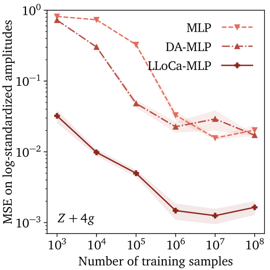
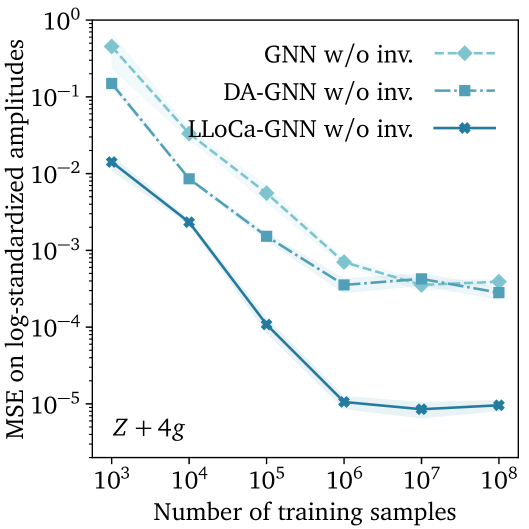
Figure 5: Comparison between LLoCa models and their non-equivariant counterparts. We consider a simple MLP (left) and a graph network that does not use additional Lorentz invariant edge features (right). The global frames for the data augmentation (DA) results are sampled as described in App. C.

More Lorentz-equivariant architectures

Following the guiding principle of our contribution, we present other architectures that are turned into Lorentz-equivariant via local canonicalization. We study the same graph network without including the Lorentz-invariant edge features $\langle p_{i},p_{j}\rangle$ as arguments for the main network. The other baseline we consider is a simple MLP with four-momenta as inputs. We do not include non-trivial frame-to-frame transformations following (10), effectively allowing only scalar message. The architecture is still Lorentz-equivariant due to Sec. 4.2. In Fig. 5 we repeat the same scaling study as presented in Sec. 5. Although these two models are not competitive with the models presented in Sec. 5, we observe significant improvements from introducing Lorentz-equivariance.

Frames-Net regularization

Besides the message representations discussed in Tab. 2, the main design choice of LLoCa is the architecture of the FramesNet $\varphi$ described in Sec. 4.5. We consider several choices and train LLoCa-Transformers on the $Z+4g$ dataset for different training dataset sizes, see Fig. 6. First, we find that the default Frames-Net (“Learnable LLoCa”) tends to overfit at larger training dataset sizes than the main network. We tackle this by using a dropout rate of 0.2 when less than $10^{5}$ training events are available (“Learnable LLoCa + Dropout”). We do not use dropout for larger training dataset sizes because we find that it affects the network performance. A similar effect can be achieved by decreasing the size of the Frames-Net (“Learnable small LLoCa”), where we use 16 instead of 128 hidden channels. However, we find that decreasing the network size slightly degrades performance in the large-data regime. We find that a Frames-Net with parameters fixed after initialization (“Fixed LLoCa”) still outperforms the non-equivariant counterpart. When little training data is available, a fixed Frames-Net combined with a dropout rate of 0.2 (“Fixed LLoCa + Dropout”) even achieves the best performance.

Constructing local reference frames

Our default approach for constructing local reference frames based on a polar decomposition is equivalent to a direct Gram-Schmidt algorithm in Minkowski space and removing the boost yields the special case of local reference frames for $\mathrm{SO}(3)$-equivariant architectures, see Sec. 4.5 and App. B. We now put these observations to the test and train LLoCa-Transformers on different training dataset sizes of the $Z+4g$ dataset, see Fig. 6. First, we find that a direct Gram-Schmidt algorithm in Minkowski space ($\mathrm{GS}^{4}$) shows very similar performance to our default polar decomposition approach (PD). The special case of $\mathrm{SO}(3)$-equivariance obtained by only including the rotation part ($\mathrm{GS}^{3}$) yields significantly worse performance due to the reduced symmetry group. All approaches show a very similar scaling behaviour with the training dataset size.

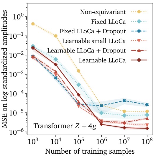
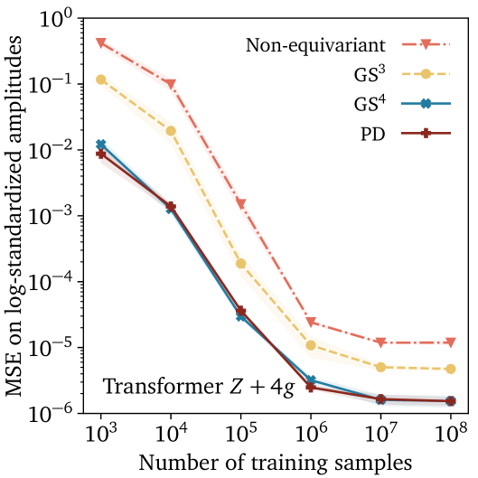
Figure 6: Design choices when constructing local reference frames. Left: Effect of the network architecture used for the Frames-Net $\varphi$. We use “Learnable LLoCa” in all other experiments, and “Learnable LLoCa + Dropout” when less than $10^{5}$ training events are available. Right: Comparison of different orthonormalization schemes. We use “PD” in all other experiments.

Attention inner product

For the scaled dot-product attention discussed in Eq. (11), we use the Minkowski product to project keys onto queries. We find that this design choice significantly outperforms the naive choice of Euclidean attention, see Tab. 4.

Table 4: Benefit of Minkowski attention compared to Euclidean attention. We show results for the LLoCa-Transformer on the full $Z+4g$ dataset.

Attention	MSE ($\times 10^{-6}$)
Euclidean	3.6 $\pm$ 0.6
Minkowski	1.5 $\pm$ 0.1

D.2 Jet tagging

More evaluation metrics

In addition to the global evaluation metrics reported in Tab. 1, we report class-wise background rejection rates in Tab. 5.

	$H\to b\bar{b}$	$H\to c\bar{c}$	$H\to gg$	$H\to 4q$	$H\to l\nu q\bar{q}^{\prime}$	$t\to bq\bar{q}^{\prime}$	$t\to bl\nu$	$W\to q\bar{q}^{\prime}$	$Z\to q\bar{q}$
	Rej50%	Rej50%	Rej50%	Rej50%	Rej99%	Rej50%	Rej99.5%	Rej50%	Rej50%
PFN Komiske et al. [2019]	2924	841	75	198	265	797	721	189	159
P-CNN [Sirunyan et al., 2020]	4890	1276	88	474	947	2907	2304	241	204
ParticleNet Qu and Gouskos [2020]	7634	2475	104	954	3339	10526	11173	347	283
ParT Qu et al. [2024]	10638	4149	123	1864	5479	32787	15873	543	402
MIParT Wu et al. [2025]	10753	4202	123	1927	5450	31250	16807	542	402
L-GATr Brehmer et al. [2024b]	12987	4819	128	2311	6116	47619	20408	588	432
Transformer (ours)	10753	3333	116	1369	4630	24390	17857	415	334
LLoCa-Transf.* (ours)	11628	4651	125	2037	5618	39216	17241	548	410
LLoCa-ParT* (ours)	11561	4640	125	2037	5900	41667	19231	552	419
LLoCa-ParticleNet* (ours)	7463	2833	105	1072	3155	10753	9302	403	306

Table 5: Background rejection rates $1/\epsilon_{B}$ for the JetClass dataset Qu et al. [2024]. For each class, $\mathrm{Rej}_{N\%}$ represents the inverse signal fraction at fixed background rejection rate $N\%$. Lorentz-equivariant methods are marked with an asterisk*. See Tab. 1 for the global accuracy and AUC.

Effect of Lorentz symmetry breaking

We follow the approach of Ref. Spinner et al. [2024], Brehmer et al. [2024b] of using fully Lorentz-equivariant models and breaking their symmetry instead of considering models that are only equivariant under the $\mathrm{SO}(2)$ symmetry of rotations around the beam direction. Note that the baseline models ParticleNet, ParT, MIParT and our Transformer are all $\mathrm{SO}(2)$-invariant, because their inputs are invariant under $\mathrm{SO}(2)$ transformations.

As described in App. C, we use two independent methods to break the Lorentz symmetry down to the $\mathrm{SO}(2)$ subgroup of rotations around the beam direction. They are (a) including features in the list of Lorentz-invariant inputs $s_{i}$ in Eq. (13) that are only invariant under the unbroken subgroup (non-invariant scalars, or NIS), and (b) including reference vectors (RV) pointing in the directions orthogonal to the unbroken subgroup as additional particles. The additional NIS and RV inputs are described in more detail in App. C. In Tab. 6 we study the effect of this design choice.

To study the impact of Lorentz symmetry breaking, we directly compare the cases of “No symmetry breaking” with only “RV”, only “NIS”, and our default of including both “RV & NIS”. The Lorentz-equivariant model that does not include any source of symmetry breaking is significantly worse and only marginally better than the non-equivariant approach, because it constrains the model to assign an equal tagging score to input jets with different physical meaning. The models trained with symmetry breaking through the “RV”, “NIS” and “RV & NIS” approaches all have a sufficient amount of symmetry breaking included, but still yield slightly different results. We also compare to a $\mathrm{SO}(3)$-equivariant model using the same reference vectors and non-invariant scalars to break the symmetry down to the unbroken subgroup of rotations around the beam direction.

Symmetry breaking	All classes		$H\to b\bar{b}$	$H\to c\bar{c}$	$H\to gg$	$H\to 4q$	$H\to l\nu q\bar{q}^{\prime}$	$t\to bq\bar{q}^{\prime}$	$t\to bl\nu$	$W\to q\bar{q}^{\prime}$	$Z\to q\bar{q}$
	Accuracy	AUC	Rej50%	Rej50%	Rej50%	Rej50%	Rej99%	Rej50%	Rej99.5%	Rej50%	Rej50%
Non-equivariant	0.855	0.9867	10753	3333	116	1369	4630	24390	17857	415	334
SO(3)-equivariant RV & NIS	0.863	0.9880	11976	4619	124	2030	5571	37037	16394	545	407
No symmetry breaking	0.856	0.9870	9756	3781	113	1660	4762	24692	15385	465	351
RV	0.861	0.9877	11494	4444	122	1923	5222	34483	17391	521	398
NIS	0.863	0.9881	11300	4630	124	1983	5249	40817	17544	547	405
RV & NIS (default)	0.864	0.9882	11628	4651	125	2037	5618	39216	17241	548	410

Table 6: Impact of symmetry breaking for jet tagging. LLoCa-Transformer accuracy, AUC, and background rejection $1/\epsilon_{B}$ for different symmetry-breaking approaches. We compare the effect of symmetry breaking with reference vectors (RV) and non-invariant scalars (NIS) with the case of no symmetry breaking as well as a non-equivariant and a $\mathrm{SO}(3)$-equivariant model (which also uses symmetry breaking with RV&NIS).

References

- Alwall et al. [2011] Johan Alwall, Michel Herquet, Fabio Maltoni, Olivier Mattelaer, and Tim Stelzer. MadGraph 5 : Going Beyond. JHEP, 06:128, 2011. doi: 10.1007/JHEP06(2011)128.
- ATLAS collaboration [2012] ATLAS collaboration. Observation of a new particle in the search for the Standard Model Higgs boson with the ATLAS detector at the LHC. Physics Letters B, 716(1):1–29, 2012.
- Aylett-Bullock et al. [2021] Joseph Aylett-Bullock, Simon Badger, and Ryan Moodie. Optimising simulations for diphoton production at hadron colliders using amplitude neural networks. Journal of High Energy Physics, 2021(8):1–30, 2021.
- Badger and Bullock [2020] Simon Badger and Joseph Bullock. Using neural networks for efficient evaluation of high multiplicity scattering amplitudes. Journal of High Energy Physics, 2020(6):1–26, 2020.
- Badger et al. [2023] Simon Badger, Anja Butter, Michel Luchmann, Sebastian Pitz, and Tilman Plehn. Loop amplitudes from precision networks. SciPost Physics Core, 6(2):034, 2023.
- Baker et al. [2024] Justin Baker, Shih-Hsin Wang, Tommaso de Fernex, and Bao Wang. An explicit frame construction for normalizing 3D point clouds. In Forty-first International Conference on Machine Learning, 2024.
- Bogatskiy et al. [2022] Alexander Bogatskiy, Timothy Hoffman, David W. Miller, and Jan T. Offermann. Pelican: Permutation equivariant and lorentz invariant or covariant aggregator network for particle physics, 2022.
- Brehmer et al. [2024a] Johann Brehmer, Sönke Behrends, Pim de Haan, and Taco Cohen. Does equivariance matter at scale? arXiv preprint arXiv:2410.23179, 2024a.
- Brehmer et al. [2024b] Johann Brehmer, Víctor Bresó, Pim de Haan, Tilman Plehn, Huilin Qu, Jonas Spinner, and Jesse Thaler. A lorentz-equivariant transformer for all of the lhc. arXiv preprint arXiv:2411.00446, 2024b.
- Bresó et al. [2024] Víctor Bresó, Gudrun Heinrich, Vitaly Magerya, and Anton Olsson. Interpolating amplitudes, 2024. URL https://arxiv.org/abs/2412.09534.
- Bronstein et al. [2021] Michael M Bronstein, Joan Bruna, Taco Cohen, and Petar Veličković. Geometric deep learning: Grids, groups, graphs, geodesics, and gauges. arXiv preprint arXiv:2104.13478, 2021.
- Butter et al. [2023] Anja Butter, Tilman Plehn, Steffen Schumann, Simon Badger, Sascha Caron, Kyle Cranmer, Francesco Armando Di Bello, Etienne Dreyer, Stefano Forte, Sanmay Ganguly, et al. Machine learning and LHC event generation. SciPost Physics, 14(4):079, 2023.
- Centre [2021] CERN Data Centre. Key facts and figures, 2021. URL https://information-technology.web.cern.ch/sites/default/files/CERNDataCentre_KeyInformation_Nov2021V1.pdf.
- CMS collaboration [2012] CMS collaboration. Observation of a new boson at a mass of 125 GeV with the CMS experiment at the LHC. Physics Letters B, 716(1):30–61, 2012.
- Cohen [2021] Taco Cohen. Equivariant Convolutional Networks. PhD thesis, University of Amsterdam, 2021.
- Dao et al. [2022] Tri Dao, Dan Fu, Stefano Ermon, Atri Rudra, and Christopher Ré. FlashAttention: Fast and memory-efficient exact attention with IO-awareness. Advances in Neural Information Processing Systems, 35:16344–16359, 2022.
- Du et al. [2024] Yuanqi Du, Limei Wang, Dieqiao Feng, Guifeng Wang, Shuiwang Ji, Carla P Gomes, Zhi-Ming Ma, et al. A new perspective on building efficient and expressive 3D equivariant graph neural networks. Advances in Neural Information Processing Systems, 36, 2024.
- Einstein [1905] Albert Einstein. Zur Elektrodynamik bewegter Körper. Annalen der Physik, 4, 1905.
- Gong et al. [2022] Shiqi Gong, Qi Meng, Jue Zhang, Huilin Qu, Congqiao Li, Sitian Qian, Weitao Du, Zhi-Ming Ma, and Tie-Yan Liu. An efficient lorentz equivariant graph neural network for jet tagging. Journal of High Energy Physics, 2022(7), July 2022. ISSN 1029-8479. doi: 10.1007/jhep07(2022)030. URL http://dx.doi.org/10.1007/JHEP07(2022)030.
- Guest et al. [2018] Dan Guest, Kyle Cranmer, and Daniel Whiteson. Deep learning and its application to LHC physics. Annual Review of Nuclear and Particle Science, 68:161–181, 2018.
- Jumper et al. [2021] John Jumper, Richard Evans, Alexander Pritzel, Tim Green, Michael Figurnov, Olaf Ronneberger, Kathryn Tunyasuvunakool, Russ Bates, Augustin Žídek, Anna Potapenko, et al. Highly accurate protein structure prediction with alphafold. nature, 596(7873):583–589, 2021.
- Kaba et al. [2023] Sékou-Oumar Kaba, Arnab Kumar Mondal, Yan Zhang, Yoshua Bengio, and Siamak Ravanbakhsh. Equivariance with learned canonicalization functions. In International Conference on Machine Learning, pages 15546–15566. PMLR, 2023.
- Kasieczka et al. [2019] Gregor Kasieczka, Tilman Plehn, Anja Butter, Kyle Cranmer, Dipsikha Debnath, Barry M Dillon, Malcolm Fairbairn, Darius A Faroughy, Wojtek Fedorko, Christophe Gay, et al. The machine learning landscape of top taggers. SciPost Physics, 7(1):014, 2019.
- Komiske et al. [2019] Patrick T Komiske, Eric M Metodiev, and Jesse Thaler. Energy flow networks: deep sets for particle jets. Journal of High Energy Physics, 2019(1):1–46, 2019.
- Langer et al. [2024] Marcel F Langer, Sergey N Pozdnyakov, and Michele Ceriotti. Probing the effects of broken symmetries in machine learning. arXiv preprint arXiv:2406.17747, 2024.
- Li et al. [2021] Feiran Li, Kent Fujiwara, Fumio Okura, and Yasuyuki Matsushita. A closer look at rotation-invariant deep point cloud analysis. In Proceedings of the IEEE/CVF International Conference on Computer Vision, pages 16218–16227, 2021.
- Lippmann et al. [2025] Peter Lippmann, Gerrit Gerhartz, Roman Remme, and Fred A Hamprecht. Beyond canonicalization: How tensorial messages improve equivariant message passing. In The Thirteenth International Conference on Learning Representations, 2025.
- Luo et al. [2022] Shitong Luo, Jiahan Li, Jiaqi Guan, Yufeng Su, Chaoran Cheng, Jian Peng, and Jianzhu Ma. Equivariant point cloud analysis via learning orientations for message passing. In Proceedings of the IEEE/CVF Conference on Computer Vision and Pattern Recognition, pages 18932–18941, 2022.
- Maˆıtre and Truong [2023] D Maître and H Truong. One-loop matrix element emulation with factorisation awareness. Journal of High Energy Physics, 2023(5):1–21, 2023.
- Maˆıtre and Truong [2021] Daniel Maître and Henry Truong. A factorisation-aware matrix element emulator. Journal of High Energy Physics, 2021(11):1–24, 2021.
- Minkowski [1908] Hermann Minkowski. Die Grundgleichungen für die elektromagnetischen Vorgänge in bewegten Körpern. Nachrichten von der Gesellschaft der Wissenschaften zu Göttingen, Mathematisch-Physikalische Klasse, 1908:53–111, 1908.
- Poincaré [1906] Henri Poincaré. Sur la dynamique de l’électron. Circolo Matematico di Palermo, 1906.
- Qu and Gouskos [2020] Huilin Qu and Loukas Gouskos. Jet tagging via particle clouds. Physical Review D, 101(5), March 2020. ISSN 2470-0029. doi: 10.1103/physrevd.101.056019. URL http://dx.doi.org/10.1103/PhysRevD.101.056019.
- Qu et al. [2024] Huilin Qu, Congqiao Li, and Sitian Qian. Particle transformer for jet tagging, 2024.
- Ruhe et al. [2023] David Ruhe, Johannes Brandstetter, and Patrick Forré. Clifford group equivariant neural networks. In Advances in Neural Information Processing Systems, volume 37, 2023.
- Salam [2010] Gavin P. Salam. Towards Jetography. Eur. Phys. J. C, 67:637–686, 2010. doi: 10.1140/epjc/s10052-010-1314-6.
- Sirunyan et al. [2020] Albert M Sirunyan et al. Identification of heavy, energetic, hadronically decaying particles using machine-learning techniques. JINST, 15(06):P06005, 2020. doi: 10.1088/1748-0221/15/06/P06005.
- Spinner et al. [2024] Jonas Spinner, Victor Bresó, Pim De Haan, Tilman Plehn, Jesse Thaler, and Johann Brehmer. Lorentz-equivariant geometric algebra transformers for high-energy physics. In Advances in Neural Information Processing Systems, volume 37, 2024. URL https://arxiv.org/abs/2405.14806.
- Touvron et al. [2021] Hugo Touvron, Matthieu Cord, Alexandre Sablayrolles, Gabriel Synnaeve, and Hervé Jégou. Going deeper with image transformers. In Proceedings of the IEEE/CVF international conference on computer vision, pages 32–42, 2021.
- Vaswani et al. [2017] Ashish Vaswani, Noam Shazeer, Niki Parmar, Jakob Uszkoreit, Llion Jones, Aidan N Gomez, Łukasz Kaiser, and Illia Polosukhin. Attention is all you need. Advances in Neural Information Processing Systems, 30, 2017.
- Villar et al. [2021] Soledad Villar, David W Hogg, Kate Storey-Fisher, Weichi Yao, and Ben Blum-Smith. Scalars are universal: Equivariant machine learning, structured like classical physics. Advances in Neural Information Processing Systems, 34:28848–28863, 2021.
- Wang et al. [2023] Hanchen Wang, Tianfan Fu, Yuanqi Du, Wenhao Gao, Kexin Huang, Ziming Liu, Payal Chandak, Shengchao Liu, Peter Van Katwyk, Andreea Deac, et al. Scientific discovery in the age of artificial intelligence. Nature, 620(7972):47–60, 2023.
- Wang and Zhang [2022] Xiyuan Wang and Muhan Zhang. Graph neural network with local frame for molecular potential energy surface. In Learning on Graphs Conference, pages 19–1. PMLR, 2022.
- Wu et al. [2025] Yifan Wu, Kun Wang, Congqiao Li, Huilin Qu, and Jingya Zhu. Jet tagging with more-interaction particle transformer*. Chin. Phys. C, 49(1):013110, 2025. doi: 10.1088/1674-1137/ad7f3d.
- Zhao et al. [2022] Chen Zhao, Jiaqi Yang, Xin Xiong, Angfan Zhu, Zhiguo Cao, and Xin Li. Rotation invariant point cloud analysis: Where local geometry meets global topology. Pattern Recognition, 127:108626, 2022.
- Zhao et al. [2020] Yongheng Zhao, Tolga Birdal, Jan Eric Lenssen, Emanuele Menegatti, Leonidas Guibas, and Federico Tombari. Quaternion equivariant capsule networks for 3D point clouds. In European conference on computer vision, pages 1–19. Springer, 2020.