Tools for Characterizing the Numerical Error of Stellar Oscillation Codes

Abstract

Stellar oscillation codes are software instruments that evaluate the normal-mode frequencies of an input stellar model. While inter-code comparisons are often used to confirm the correctness of calculations, they are not suitable for characterizing the numerical error of an individual code. To address this issue, we introduce a set of tools — ‘error measures’ — that facilitate this characterization. We explore the behavior of these error measures as calculation parameters, such as the number of radial grid points used to discretize the oscillation equations, are varied; and we summarize this behavior via an idealized error model. While our analysis focuses on the GYRE code, it remains broadly applicable to other oscillation codes.

tablenum

1 Introduction

Recent space photometry missions, including MOST (Walker et al., 2003), CoRoT (Baglin et al., 2006), Kepler (Borucki et al., 2010), and TESS (Ricker et al., 2014), have provided time-series measurements of oscillations in myriad stars spanning the Hertzsprung-Russell diagram. The technique of asteroseismology (e.g., Aerts et al., 2010) can leverage these data into quantitative constraints on the global properties (mass, radius, age, metallicity, etc.) and detailed interior structures of the stars observed.

A key ingredient in asteroseismic modeling is a stellar oscillation code, a software instrument that evaluates the normal-mode frequencies of an input stellar model. Many such codes are described in the literature; examples include MAD (Dupret, 2001), LP-PUL (Córsico & Benvenuto, 2002), PULSE (Brassard & Charpinet, 2008), ADIPLS (Christensen-Dalsgaard, 2008), GraCo (Moya & Garrido, 2008), NOSC (Provost, 2008), OSC (Scuflaire et al., 2008), filou (Suárez & Goupil, 2008), LNAWENR (Suran, 2008), CAFEIN (Valsecchi et al., 2013), and GYRE (Townsend & Teitler, 2013; Townsend et al., 2018; Goldstein & Townsend, 2020; Sun et al., 2023). Given the community’s increasing reliance on these complex software packages, it is important to verify that they yield results that are not only precise but also accurate.

Historically, a number of papers have examined the problem of code verification. In considering the oscillations of polytropic models, Mullan & Ulrich (1988) employ a convergence criterion that the change in mode frequencies, upon increasing the number of radial grid points used to discretize the oscillation equations, drops below a prescribed threshold. Such an approach can ensure that frequencies are precise, but does not by itself also guarantee accuracy. In a subsequent paper, Christensen-Dalsgaard & Mullan (1994) expand on this work by undertaking a comprehensive comparison between the polytrope-model frequencies evaluated by a pair of independent oscillation codes. More recently, Moya et al. (2008) compare many of the codes cited above, as applied to realistic stellar models.

Inter-code comparisons provide confidence that oscillation codes are yielding reliable results. However, their utility is limited when it comes to characterizing the numerical error of an individual code — for instance, diagnosing the various mechanisms that contribute toward this error, and exploring whether these mechanisms behave as expected from theoretical considerations. Such characterizations can potentially highlight hidden bugs, and are key to deciding if and how the code can further be improved.

Within this context, the present paper introduces a set of tools for characterizing the numerical error of oscillation codes. We introduce these tools — ‘error measures’ — in Section 2, and demonstrate their application to the GYRE code in Section 3. We summarize our findings in Section 4, and discuss some of the practicalities of using the tools in the context of asteroseismic studies.

2 Error measures

The numerical error of an oscillation code can in principle be quantified by comparing the code’s outputs (eigenfrequencies, eigenfunctions, etc.) against exact solutions. In practice, however, the latter are known only for the simple and quite artificial case of the homogeneous compressible sphere (see Pekeris, 1938). To proceed, therefore, we heed these words from Christensen-Dalsgaard & Berthomieu (1991): “The only practical way of estimating the numerical error in the computed frequencies is to compare results obtained with different numbers of mesh [grid] points”.

The general process is straightforward: run a code multiple times while varying the number of radial grid points $N$, and explore how its outputs change with $N$. As a straightforward example, one might follow Mullan & Ulrich (1988) and focus on how the frequency $\sigma$ of a given mode depends on $N$. However, as we already mention above, this approach ensures precision but does not guarantee accuracy. The problem lies with the choice of $\sigma$ as the output to monitor; by itself, it furnishes no indication that it lies close to the correct value. To address this, we introduce the concept of an error measure $\mathcal{E}$, fulfilling the following criteria:

1. $\mathcal{E}$ must be calculable from the outputs of the oscillation code;

2. $\mathcal{E}$ must be insensitive to non-physical quantities such as the normalization of eigenfunctions;

3. $\mathcal{E}$ must approach zero as numerical solutions approach exact solutions of the oscillation equations.

The last criterion is key to ensuring that precision and accuracy go hand-in-hand. In the subsections that follow, we introduce three specific definitions of the error measure. To keep the presentation compact, we defer much of the detailed mathematical formalism to Appendix A.

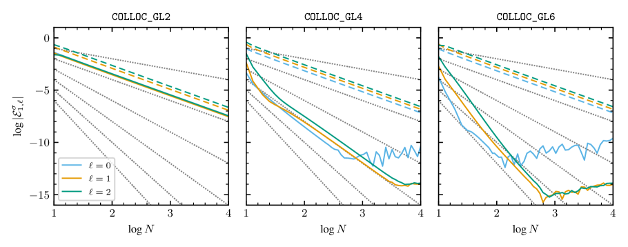
Figure 1: The frequency error measure $\mathcal{E}^{\sigma}_{n,\ell}$ plotted as a function of the number of grid points $N$, for $n=1$, $\ell=0,1,2$ modes of the $n_{\rm poly}=1$ polytrope. The panels show differing choices of the discretization scheme, indicated at top. Solid (dashed) lines show data evaluated using the Newton-Coates (trapezoidal) quadrature schemes. To help asses the rate of convergence, the dotted lines indicate $|\mathcal{E}^{\sigma}_{n,\ell}|=N^{-j}$ for $j=1,\ldots,6$.

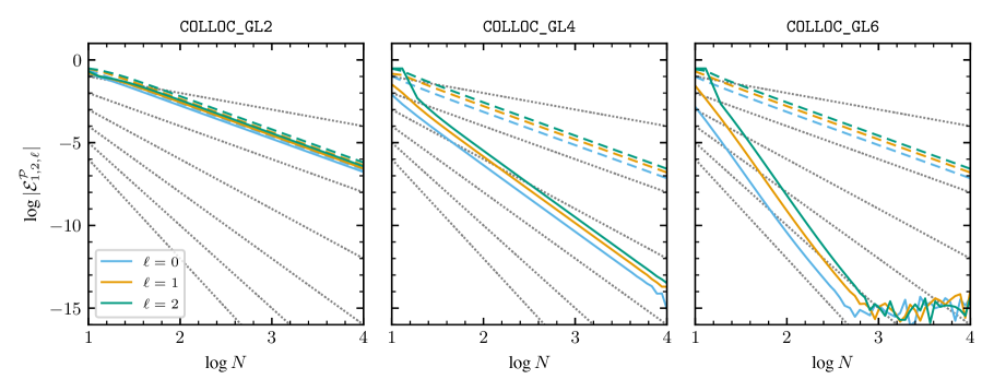
Figure 2: As in Fig. 1, except that the orthogonality error measure $\mathcal{E}^{\mathcal{P}}_{n,n^{\prime},\ell}$ is now plotted for $(n,n^{\prime})=(1,2)$ modes.

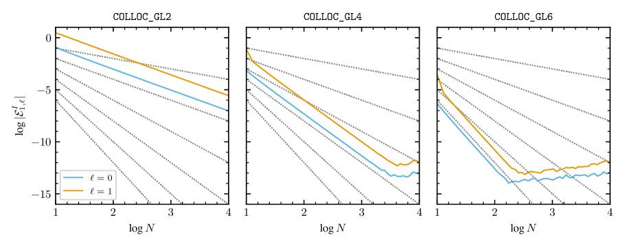
Figure 3: As in Fig. 1, except that the first-integral error measure $\mathcal{E}^{I}_{n,\ell}$ is now plotted for $n=1$ modes. Note that this error measure is defined only for $\ell=0,1$, and thus no $\ell=2$ curve is shown.

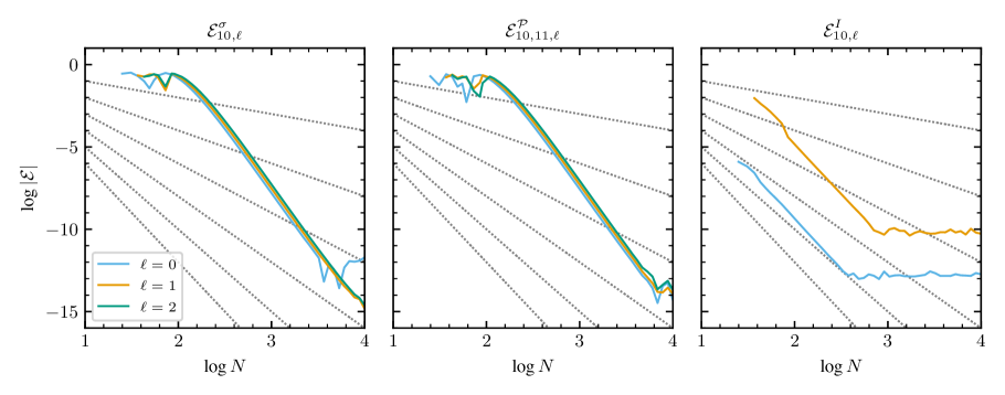
Figure 4: The $\mathcal{E}^{\sigma}_{n,\ell}$, $\mathcal{E}^{\mathcal{P}}_{n,n^{\prime},\ell}$ and $\mathcal{E}^{I}_{n,\ell}$ error measures plotted as a function of the number of grid points $N$, for $(n,n^{\prime})=(10,11)$, $\ell=0,1,2$ modes of the $n_{\rm poly}=1$ polytrope. All calculations use the COLLOC_GL6 discretization scheme. The dotted lines are the same as in previous figures. No data are shown at small $N$ because GYRE is unable to find the requisite modes on such coarse grids.

2.1 Frequency error measure

As discussed in Appendix A.2, the frequency of a mode can be evaluated from various integrals over its eigenfunctions. For numerical solutions, this ‘integral’ frequency will not agree exactly with the eigenfrequency output by the oscillation code, and we introduce the frequency error measure

$$\mathcal{E}^{\sigma}_{n,\ell}\equiv\frac{\sigma^{\rm e}_{n,\ell}-\sigma^{\rm i}_{n,\ell}}{\sigma^{\rm e}_{n,\ell}}$$ (1)

to quantify their relative difference. Here, $\sigma^{\rm e}_{n,\ell}$ is the eigenfrequency output by the code, and $\sigma^{\rm i}_{n,\ell}$ is the integral frequency evaluated using equation (A8); throughout, the subscripts $n$ and $\ell$ denote the radial order and harmonic degree, respectively, of the mode.

2.2 Orthogonality error measure

As discussed in Appendix A.3, the displacement eigenfunctions of a pair of oscillation modes with the same harmonic degree but different radial orders ($n,n^{\prime}$) are orthogonal if the surface term (A6) satisfies $\mathcal{S}_{n,n^{\prime},\ell}=\mathcal{S}_{n^{\prime},n,\ell}^{\ast}$. Numerical solutions will not satisfy this property exactly, and we introduce the orthogonality error measure

$$\mathcal{E}^{\mathcal{P}}_{n,n^{\prime},\ell}\equiv\frac{\mathcal{P}_{n,n^{\prime},\ell}}{\left(\mathcal{P}_{n,n,\ell}\,\mathcal{P}_{n^{\prime},n^{\prime},\ell}\right)^{1/2}},$$ (2)

to quantify the discrepancy; here, the inner product $\mathcal{P}_{n,n^{\prime},\ell}$ is defined in equation (A4). In accordance with criterion (ii), above, the denominator ensures that this measure remains independent of the arbitrary normalization of eigenfunctions.

2.3 First-Integral Error Measure

As shown by Takata (2006a), the oscillation equations for radial ($\ell=0$) and dipole ($\ell=1$) modes admit first integrals that vanish everywhere for solutions that remain regular at the origin. Once again, numerical solutions to the equations will not satisfy this property exactly, and we introduce the first-integral error measure

$$\mathcal{E}^{I}_{n,\ell}\equiv\frac{\max(I_{n,\ell})-\min(I_{n,\ell})}{\mathcal{P}_{n,n,\ell}^{1/2}}$$ (3)

to quantify the discrepancy. Here, $I_{n,\ell}$ ($\ell=0,1$) are the first integrals defined in equations (42) and (43) of Takata (2006a) for radial and dipole cases, respectively; and the $\min()$ and $\max()$ operators denote the minimum and maximum value attained over all points of the radial grid. As with equation (2), the denominator ensures that this measure is independent of eigenfunction normalization.

3 Calculations

For a variety of stellar models, we explore how the error measures introduced above behave as a function of the number of radial grid points $N$. We use release 8.0 of the GYRE code, which includes support for the evaluated models discussed in Section 3.1. At the stellar surface $r=R$ we impose the zero-pressure mechanical boundary condition

$$\delta\tilde{P}_{n,\ell}\equiv\tilde{P}_{n,\ell}^{\prime}-g\,\rho\,\tilde{\xi}_{{\rm r};n,\ell}=0,$$ (4)

together with the potential boundary condition

$$\frac{\operatorname{d}\!{\tilde{\Phi}_{n,\ell}^{\prime}}}{\operatorname{d}\!{r}}+\frac{\ell+1}{r}\tilde{\Phi}_{n,\ell}^{\prime}=-4\pi\,G\,\rho\,\tilde{\xi}_{{\rm r};n,\ell}$$ (5)

(see, e.g., Cox, 1980). Together, these boundary conditions mean that $\mathcal{S}_{n,n^{\prime},\ell}=\mathcal{S}_{n^{\prime},n,\ell}^{\ast}$ (see equation A14), and thus eigenfunctions should be orthogonal. We briefly discuss the impact of other boundary-condition choices in Section 4.

With the exception of a few special cases that we highlight when necessary, the grids employed by GYRE consist of $N=6K+1$ points uniformly distributed in fractional radius $0\leq x\equiv r/R\leq 1$, where $K$ is an integer. This choice allows us to evaluate integrals (for instance, those appearing in equations A8 and A13) using composite 7-point Newton-Coates quadrature (Press et al., 1992) across $K$ sub-intervals. The motivation here is to ensure that the quadrature truncation error remains small in comparison to the other sources of numerical error arising in the calculations.

3.1 Evaluated models

We first consider stellar models where the internal structure can be evaluated from closed-form expressions. The most simple are the polytropes with indices $n_{\rm poly}=0$, 1 and 5; in these cases, GYRE calculates the structure of the model on-the-fly using the analytic solutions to the Lane-Emden equation (see, e.g., Horedt, 2004). Setting aside the $n_{\rm poly}=0$ case (which corresponds to the homogeneous compressible sphere, and as discussed above is special), in this section we focus on the $n_{\rm poly}=1$ and $n_{\rm poly}=5$ polytropes, together with a composite polytrope formed from a combination of these.

3.1.1 $n_{\rm poly}=1$ polytrope

We begin by exploring the behavior of the error measures in the case of an $n_{\rm poly}=1$ polytrope. For this, and for all other polytrope models considered, we adopt a canonical first adiabatic index $\Gamma_{1}=5/3$. Figure 1 plots the frequency error measure $\mathcal{E}^{\sigma}_{n,\ell}$ as a function of $N$, for $n=1$, $\ell=0,1,2$ modes. The three panels correspond to different choices of the numerical scheme used to discretize the oscillation equations onto the radial grid. GYRE implements a multiple-shooting approach where the relationship between dependent variables at adjacent grid points is treated as an initial-value problem (IVP). The COLLOC_GLi schemes ($i=2,4,6$) referenced in the figure solve this IVP using Gauss-Legendre collocation (e.g., Ascher et al., 1995), an implicit Runge-Kutta method with $i/2$ intermediate stages.

The frequency error measures plotted in each panel display broadly similar behavior. Initially, they decay rapidly with increasing $N$, asymptoting toward a scaling $\mathcal{E}^{\sigma}_{n,\ell}\sim N^{-i}$. This continues until $\mathcal{E}^{\sigma}_{n,\ell}$ drops to $\approx 10^{-11}$ ($\approx 10^{-14}$) for the radial (respectively, non-radial) modes; beyond these limits, the error measures grow approximately linearly with $N$, with significant variability from one value to the next.

The asymptotic-decay regime arises when the truncation error of the discretization scheme makes the dominant contribution toward $\mathcal{E}^{\sigma}_{n,\ell}$. Theoretically, the local truncation error of the COLLOC_GL$i$ scheme is $O(h^{i+1})$, where $h=(N-1)^{-1}\approx N^{-1}$ is the spacing between adjacent grid points. This yields a global error scaling as $\sim N(N-1)^{-i-1}\approx N^{-i}$, as seen in each panel of the figure.

The switch to the slow-growth regime occurs when the dominant contribution toward $\mathcal{E}^{\sigma}_{n,\ell}$ transitions to round-off error. GYRE performs all calculations using IEEE 754 binary64 floating-point arithmetic, which has a 53-bit significand and therefore suffers a relative rounding error of up to $2^{-53}\approx${10}^{-16}$$ during each arithmetic operation. The round-off errors from a sequence of arithmetic operations accumulate approximately in proportion to the operation count, which in GYRE’s case scales with $N$ — hence, the approximately linear growth of the error measures plotted in the figure, once accumulated round-off error becomes dominant.

The dashed lines in Fig. 1 show the consequence of using trapezoidal quadrature to evaluate the integrals in equation (A8), instead of the Newton-Coates scheme described previously. While the output from GYRE remains unaltered by this choice, the frequency error measure in the asymptotic-decay regime now behaves as $\mathcal{E}^{\sigma}_{n,\ell}\sim N^{-2}$, because the $O(h^{3})$ local truncation error of trapezoidal quadrature dominates the truncation error of the discretization schemes [for comparison, the local truncation error of the Newton-Coates quadrature scheme is $O(h^{9})$].

Fig. 1 confirms that GYRE performs as expected, although the radial mode seems to be considerably more affected by round-off error than the other modes, which warrants further investigation. Continuing our analysis, Figs. 2 and 3 reprise Fig. 1 by plotting $\mathcal{E}^{\mathcal{P}}_{1,2,\ell}$ and $\mathcal{E}^{I}_{1,\ell}$, respectively, as a function of $N$. In each case, the same general behavior as before is seen: error measures decaying rapidly with the expected asymptotic scalings, and then slowly growing when round-off error takes over.

So far we focus on $n=1$ modes, whose eigenfunctions vary slowly with radius. As a final look at the $n_{\rm poly}=1$ polytrope, Fig. 4 reprises the right-hand (COLLOC_GL6) panels of the previous figures, but now considering modes with radial orders $(n,n^{\prime})=(10,11)$ (in the interests of brevity, we no longer show the results from calculations using the COLLOC_GL2 or COLLOC_GL4 schemes). The same general behavior as before is seen, but for the frequency and orthogonality error measures the approach toward the asymptotic $\mathcal{E}\sim N^{-6}$ scaling is delayed until larger $N$ is reached. This is a consequence of the more-oscillatory eigenfunctions of the high-order modes; smaller $h$ is needed to resolve the eigenfunctions and realize the expected $O(h^{7})$ local truncation error of the discretization scheme.

3.1.2 $n_{\rm poly}=5$ Polytrope

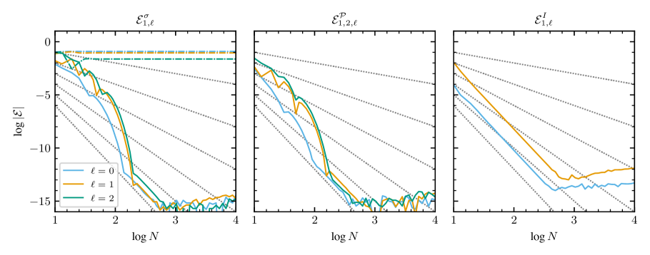
Figure 5: As in Fig. 4, but now for $(n,n^{\prime})=(1,2)$, $\ell=0,1,2$ modes of the $n_{\rm poly}=5$ polytrope. In the left-hand panel, the dot-dashed lines show the impact of neglecting the surface term $\mathcal{S}_{n,n,\ell}$ term in equation (1).

To explore the impact of a finite surface density, we now consider an $n_{\rm poly}=5$ polytrope truncated at the point where the Lane-Emden dependent variable reaches the value $\vartheta=0.2$. This implies a density $\rho_{\rm s}=0.2^{5}\,\rho_{\rm c}$ at the stellar surface (where $\rho_{\rm c}$ is the central density), meaning that the surface term $\mathcal{S}_{n,n^{\prime},\ell}$ does not generally vanish — although, with the zero-pressure boundary condition (4), it remains the case that $\mathcal{S}_{n,n^{\prime},\ell}=\mathcal{S}_{n^{\prime},n,\ell}^{\ast}$ (see the brief discussion following equation A14).

For this model, Fig. 5 reprises the COLLOC_GL6 panels of Figs. 1–3. The error measures are in line with the expectations established by the $n_{\rm poly}=1$ case, although in the left-hand and center panels the $\mathcal{E}\sim N^{-6}$ asymptotic scalings are not reached until $N\gtrsim 100$. In the left-hand panel, the dot-dashed lines reveal the consequence of neglecting the surface term: once $N\gtrsim 30$, $\mathcal{E}^{\sigma}_{n,\ell}$ shows no appreciable change with further increase in $N$, indicating that the defect introduced by this neglect has become the dominant contributor toward the frequency error measure.

3.1.3 Composite $n_{\rm poly}=5,1$ polytrope

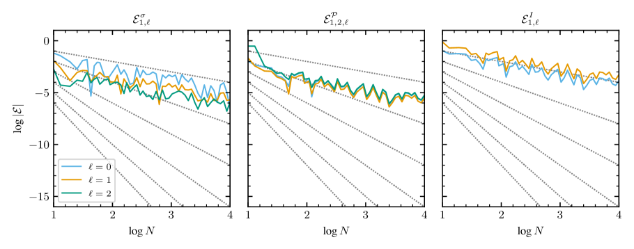
Figure 6: As in Fig. 5, but now for $(n,n^{\prime})=(1,2)$, $\ell=0,1,2$ modes of the $n_{\rm poly}=5,1$ composite polytrope.

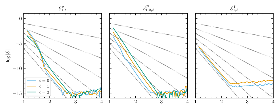
Figure 7: As in Fig. 6, except that a pair of sub-grids linked at the core-envelope boundary ($x_{\rm b}\approx 0.577$) is used.

The two polytrope models examined so far are characterized by a smoothly varying interior structure. To explore the impact of sharp structural features, we now consider a composite polytrope constructed by matching analytic solutions for an $n_{\rm poly}=5$ core and an $n_{\rm poly}=1$ envelope (see Eggleton et al., 1998, for details). Although density and pressure are continuous throughout this model, there is a jump in the density gradient and hence the Brunt-Väisälä frequency at the core-envelope boundary, which we chose to place at radial coordinate $x_{\rm b}=3^{-1/2}\approx 0.577$.

Figure 6 reveals that the error measures for this model behave quite differently than with the previous ones. In each panel, the data are noisy but follow the trend $\mathcal{E}\sim N^{-1}$. This slowed convergence is a consequence of the Brunt-Väisälä frequency jump. As shown by Gear & Østerby (1984), an order-$q$ discontinuity in the coefficients of an IVP introduces a local $O(h^{q})$ error in numerical solutions that do not resolve the discontinuity. In the present case $q=1$, leading to a $\sim N^{-1}$ contribution toward the error measures that quickly comes to dominate other sources of error. The noise arises because certain specific choices of $N$ place a grid point close to $x_{\rm b}$, somewhat mitigating the problem.

The fix here is simple: we split the grid into two sub-grids linked at the core-envelope boundary; the first spans $x\in[0,x_{\rm b}]$, the second $x\in[x_{\rm b},1]$, and solutions are required to be continuous across the boundary. Within each sub-grid, points are distributed as described in Section 3. Figure 7 demonstrates that this approach successfully eliminates the error from the discontinuity, allowing the expected $\mathcal{E}\sim N^{-6}$ scalings to emerge.

3.2 Interpolated models

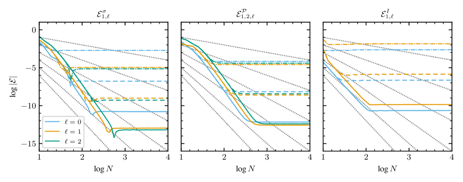
Figure 8: The $\mathcal{E}^{\sigma}_{n,\ell}$, $\mathcal{E}^{\mathcal{P}}_{n,n^{\prime},\ell}$ and $\mathcal{E}^{I}_{n,\ell}$ error measures plotted as a function of the number of grid points $N$, for $(n,n^{\prime})=(1,2)$, $\ell=0,1,2$ modes of the tabulated $n_{\rm poly}=3$ polytrope. The number of tabulation points is $M=11$ (dot-dashed), $M=101$ (dashed) and $M=1001$ (solid). The black dotted lines are the same as in previous figures.

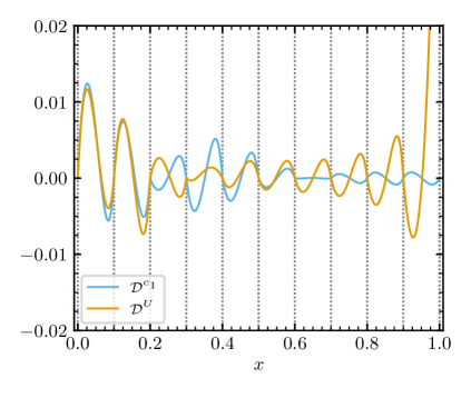
Figure 9: The defects $\mathcal{D}^{c_{1}}$ and $\mathcal{D}^{U}$ plotted as a function of fractional radius $x\equiv r/R$ for the tabulated $n_{\rm poly}=3$ polytrope with $M=11$ points. The vertical dotted lines mark these points’ abscissae.

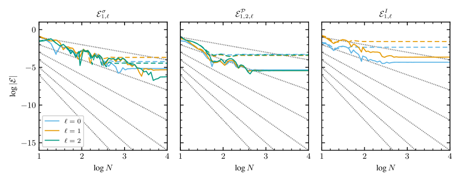
Figure 10: As in Fig. 8, but now showing results from the solar-like MESA model. The number of tabulation points is $M=389$ (dashed) and $M=3621$ (solid).

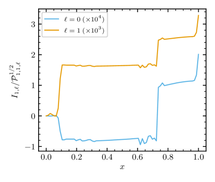
Figure 11: The first integral $I_{n,\ell}$ plotted as a function of fractional radius $x\equiv r/R$ for $n=1$, $\ell=0,1$ modes of the solar-like MESA model with $M=3621$ tabulation points.

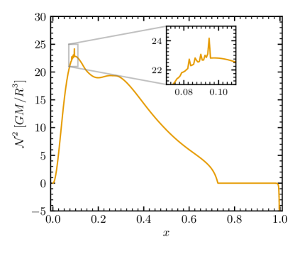
Figure 12: The square of the Brunt-Väisälä frequency $\mathcal{N}^{2}$ plotted as a function of fractional radius $x\equiv r/R$ for the solar-like MESA model with $M=3621$ tabulation points.

The analytic stellar models considered so far are helpful for illustrating the behavior of the error measures, but they are not representative use-cases for oscillation codes. More typically, a model is supplied to a code as a tabulation of various structural quantities throughout the interior of the star. In general, the radial grid of this tabulation does not match that used to discretize the oscillation equations, and some kind of interpolation is therefore required. These interpolated models are the focus of the present section.

3.2.1 $n_{\rm poly}=3$ polytrope

We first consider an $n_{\rm poly}=3$ polytrope tabulated on a uniform $M$-point radial grid. The tabulation consists of three set of values: $\{\xi_{j}\}$ ($j=1,2,\ldots,M$) representing the independent variable in the Lane-Emden equation, $\{\vartheta_{j}\}$ representing the corresponding dependent variable, and $\{\vartheta^{\prime}_{j}\}$ representing its first derivative. These data are calculated by applying the LSODAR differential-equation solver from ODEPACK (Hindmarsh, 1983) to the Lane-Emden equation, with a relative tolerance parameter $10^{-15}$. They are used by GYRE to construct piecewise cubic Hermite interpolants for both $\vartheta(\xi)$ and $\vartheta^{\prime}(\xi)$, allowing the stellar structure to be evaluated at locations that fall between the tabulation points.

Figure 8 plots the three error measures as a function of $N$, for tabulations composed of $M=11$, 101 and 1001 points. All three error measures initially decay rapidly, asymptoting toward the expected $\mathcal{E}\sim N^{-6}$ scalings, before plateauing at constant values. This stalled convergence is a consequence of the model interpolation: although the cubic interpolants exactly satisfy the Lane-Emden equation at the tabulation points, elsewhere they do not. Therefore, the model is slightly inconsistent with the stellar structure equations.

To illustrate the inconsistencies, we introduce the defects

$$\mathcal{D}^{c_{1}} \equiv\frac{\operatorname{d}\!{\ln c_{1}}}{\operatorname{d}\!{\ln x}}-\left(3-U\right),$$ (6)

$$\mathcal{D}^{U} \equiv\frac{\operatorname{d}\!{\ln U}}{\operatorname{d}\!{\ln x}}-\left(-\frac{V}{\Gamma_{1}}-A^{\ast}-U+3\right)$$

(here, $V$, $A^{\ast}$, $U$ and $c_{1}$ are the coefficients appearing in the dimensionless oscillation equations; see, e.g., Unno et al., 1989). These defects are derived from equations (20) and (21), respectively, of Takata (2006a), in such a way that they both vanish when the equilibrium stellar structure locally conserves mass. Figure 9 plots the defects as a function of $x$, for the $n_{\rm poly}=3$ polytrope tabulated with $M=11$ points. With the exception of the tabulation points (where $\mathcal{D}^{c_{1}}=\mathcal{D}^{U}=0$ by construction), it is generally the case that the defects are non-zero, highlighting the breakdown of mass conservation.

The net effect of this breakdown is to introduce additional terms on the right-hand side of the error measures (1–3), that are independent of $N$ but decrease with increasing $M$ because finer tabulations reduce the magnitude of both $\mathcal{D}^{c_{1}}$ and $\mathcal{D}^{U}$. For the data shown in the figure, switching from $M=11$ to $M=101$, and likewise from $M=101$ to $M=1001$, yields a $\approx 10^{-4}$ reduction in the error-measure plateaus, indicating that the errors from interpolation inconsistency scale as $\sim M^{-4}$.

3.2.2 MESA model

We now consider models constructed using release 24.03.01 of the MESA stellar evolution code (Paxton et al., 2011, 2013, 2015, 2018, 2019; Jermyn et al., 2023). We evolve a $1\text{\,}\mathrm{M}_{\odot}$ solar-metallicity star from the zero-age main sequence until its luminosity reaches $1\text{\,}\mathrm{L}_{\odot}$, providing a simple approximation to the present-day Sun. We repeat this exercise for two different choices of MESA’s grid refinement parameter, mesh_delta_coeff = 2.0 and mesh_delta_coeff = 0.2, leading to tabulation with $M=389$ and $M=3621$ points, respectively. From these data, GYRE constructs piecewise cubic monotonic interpolants (Steffen, 1990) for $V_{2}\equiv x^{-2}V$, $A^{\ast}$, $U$, $c_{1}$ and $\Gamma_{1}$.

Figure 10 repeats the $n_{\rm poly}=3$ calculations for the two MESA models. The error measures exhibit the same stalled convergence as in Fig. 8, which again is a consequence of the model interpolation (although now the error-measure plateau scales as $\sim M^{-2}$). However, prior to the stall the error measures decrease as $\sim N^{-2}$, albeit with significant noise. This behavior is reminiscent of Fig. 6, where the unresolved structural discontinuity in the composite polytrope results in slowed convergence. To examine what features in the MESA models might be responsible for this behavior, Fig. 11 plots the first integrals $I_{n,\ell}$ as a function of $x$ for the $n=1$, $\ell=0,1$ modes of the $M=389$ model, discretized on a grid with $N=77$ points. At three locations $x\approx 0.09,0.73,0.99$ the first integrals change rapidly, resulting in significant contributions toward the $\mathcal{E}^{I}_{n,\ell}$ error measure. Examining the model structure, each of these locations can be identified with features in the Brunt-Väisälä frequency profile (plotted in Fig. 12) that prove challenging to GYRE:

• At $x=0.09$ there are small-scale oscillations in $\mathcal{N}^{2}$. These arise from corresponding fluctuations in the gradient of the mean molecular weight, produced by the retreating boundary of a transient convective core during early main-sequence evolution.

• At $x=0.73$, there is an abrupt change in the gradient of $\mathcal{N}^{2}$. This arises from transition between the radiative interior ($\mathcal{N}^{2}>0$) and convective envelope ($\mathcal{N}^{2}\approx 0$).

• At $x=0.99$, $\mathcal{N}^{2}$ grows rapidly to large, negative values. This arises from the transition to inefficient, highly super-adiabatic convection in the surface layers.

Each of these features appear to GYRE as order-2 discontinuities in $A^{\ast}\equiv rg^{-1}\mathcal{N}^{2}$, and therefore introduces additional contributions $\sim N^{-2}$ toward the error measures that result in the slowed convergence seen in Fig. 10. In principle, a judicious choice of grid-point distribution can eliminate these contributions, as was successfully done with the composite polytrope in Section 3.1.3. However, while an optimized grid may accelerate the convergence of the error measures at small $N$, it has no effect on the plateaus seen in Fig. 10 toward larger $N$. We confirm this by repeating the calculations using GYRE’s built-in grid-refinement strategies, which place grid points based on the behavior of both the equilibrium stellar structure and the eigenfunctions. This results in no significant reduction in the error measure plateaus. We are therefore left with the conclusion that only way to push down these plateaus is to use models with finer (larger-$M$) tabulations.

4 Summary & Discussion

In the previous sections we introduce three measures, $\mathcal{E}^{\sigma}_{n,\ell}$, $\mathcal{E}^{\mathcal{P}}_{n,n^{\prime},\ell}$, and $\mathcal{E}^{I}_{n,\ell}$, as tools for characterizing the numerical error in solutions to the oscillation equations. For a variety of stellar models, we explore how these error measures respond to changes in the number of radial grid points $N$ used to discretize the oscillation equations, and/or the number of points $M$ in the tabulation of the stellar structure. To summarize the results from this investigation, we propose an idealized model for the behavior of the error measures as a function of $N$ and $M$:

$$|\mathcal{E}|\approx a_{\rm d}N^{-b_{\rm d}}+a_{\rm q}N^{-b_{\rm q}}+a_{\rm c}N^{-b_{\rm c}}+a_{\rm r}N+a_{\rm i}M^{-b_{\rm i}}.$$ (7)

Each term on the right-hand side represents a particular source of numerical error, with the $a$ coefficients setting the magnitude of the error and the $b$ coefficients determining its scaling with $N$ or $M$. In detail:

• the $a_{\rm d}N^{-b_{\rm d}}$ term represents the truncation error arising from the discretization of the oscillation equations. For a discretization scheme with local error $O(h^{i+1})$, $b_{\rm d}=i$.

• the $a_{\rm q}N^{-b_{\rm q}}$ term represents the truncation error arising from the quadrature used to evaluate the integral terms in the definitions of $\mathcal{E}^{\sigma}_{n,\ell}$ and $\mathcal{E}^{\mathcal{P}}_{n,n^{\prime},\ell}$. For a quadrature scheme with local error $O(h^{i+1})$, $b_{\rm q}=i$. The $\mathcal{E}^{I}_{n,\ell}$ error measure does not require quadrature, and so has $a_{\rm q}=0$.

• the $a_{\rm c}N^{-b_{\rm c}}$ term represents the error arising from the lowest-order discontinuity (or discontinuities) in the equilibrium stellar structure. If this discontinuity has an order $q$, then $b_{\rm c}=q$.

• the $a_{\rm r}N$ term represents the accumulated round-off error.

• the $a_{\rm i}M^{-b_{\rm i}}$ term represents the inconsistencies arising from interpolation of tabulated models. Evaluated models do not require interpolation, and so have $a_{\rm i}=0$.

This model does not account for calculation mistakes — for instance, neglecting non-zero surface terms when evaluating $\mathcal{E}^{\sigma}_{n,\ell}$ (see the dot-dashed curves in the left-hand panels of Figs. 5). Moreover, it is intended to be descriptive rather than prescriptive — a way of understanding the behavior of error measures, rather than predicting this behavior a priori.

Although our calculations focus exclusively on the GYRE code, other oscillation codes can benefit from a similar exploration of the error measures’ functional dependence on $N$ and $M$. In addition to verifying basic code correctness, such exercises can furnish a mechanism for selecting $N$, $M$ values that strike an appropriate balance between computational cost and accuracy. In this context, we expect smaller $\mathcal{E}$ to correspond to more-accurate solutions; however, to place this connection on a more quantitative footing, it behooves us to consider the semantics of each error measure — what actually is being measured?

To clarify the meaning of the frequency error measure, we write the $\sigma^{\rm e}_{n,\ell}$ and $\sigma^{\rm i}_{n,\ell}$ terms appearing on the right-hand side of equation (1) as the sum of the exact frequency $\sigma_{n,\ell}$ and a numerical error:

$$\sigma^{\rm e}_{n,\ell}=\sigma_{n,\ell}+\Delta\sigma^{\rm e}_{n,\ell},\qquad\sigma^{\rm i}_{n,\ell}=\sigma_{n,\ell}+\Delta\sigma^{\rm i}_{n,\ell}.$$ (8)

Then, equation (1) becomes

$$\mathcal{E}^{\sigma}_{n,\ell}=\frac{\Delta\sigma^{\rm e}_{n,\ell}-\Delta\sigma^{\rm i}_{n,\ell}}{\sigma_{n,\ell}}$$ (9)

where we have neglected terms that have a combined error order of second or beyond. From this, we can establish the inequality

$$|\mathcal{E}^{\sigma}_{n,\ell}|\leq 2\max\left(\left|\frac{\Delta\sigma^{\rm e}_{n,\ell}}{\sigma_{n,\ell}}\right|,\left|\frac{\Delta\sigma^{\rm i}_{n,\ell}}{\sigma_{n,\ell}}\right|\right),$$ (10)

and so the frequency error measure sets a lower bound on the magnitude of the relative error in $\sigma^{\rm e}_{n,\ell}$ or $\sigma^{\rm i}_{n,\ell}$, whichever is greater. Turning this statement around, if it is required that the relative error in the eigenfrequency be less than some threshold $E$, then it is necessary that $|\mathcal{E}^{\sigma}_{n,\ell}|\leq 2E$. Unfortunately, this condition is not also sufficient; circumstances situations can potentially arise where $|\mathcal{E}^{\sigma}_{n,\ell}|$ is significantly smaller than $E$, but the relative errors in both $\sigma^{\rm e}_{n,\ell}$ and $\sigma^{\rm i}_{n,\ell}$ remain larger than $E$.

The situation is somewhat improved in cases where the surface term satisfies $\mathcal{S}_{n,n^{\prime},\ell}=\mathcal{S}_{n^{\prime},n,\ell}^{\ast}$ — for instance, due to adoption of the zero-pressure boundary condition (4). The variational principle then predicts that $(\Delta\sigma^{\rm i}_{n,\ell}/\sigma_{n,\ell})\sim(\Delta\sigma^{\rm e}_{n,\ell}/\sigma_{n,\ell})^{2}$. In the limit $|\Delta\sigma^{\rm e}_{n,\ell}/\sigma_{n,\ell}|\ll 1$, the second term in the numerator of equation (9) can be neglected, and equation (10) then reduces to

$$|\mathcal{E}^{\sigma}_{n,\ell}|\approx\left|\frac{\Delta\sigma^{\rm e}_{n,\ell}}{\sigma_{n,\ell}}\right|,$$ (11)

indicating that the frequency error measure is the relative error in the eigenfrequency. However, a word of caution here (echoing the remarks in section 4 of Christensen-Dalsgaard et al., 1979): $\Delta\sigma^{\rm i}_{n,\ell}$ includes a contribution from the truncation error that arises when evaluating the integrals in equation (A8), and this contribution is not subject to the variational principle. Therefore, neglecting $\Delta\sigma^{\rm i}_{n,\ell}$ requires that a sufficiently accurate quadrature scheme be used.

Interpreting the orthogonality error measure is rather more straightforward: it represents the cosine of the angle in the Hilbert space defined by the inner products $\mathcal{P}_{n,n^{\prime},\ell}$. This information is useful when expanding solutions to certain problems in a superposition of eigenfunctions — for instance, when calculating the response of a star to tidal forcing by a companion object (see, e.g., Burkart et al., 2012; Fuller & Lai, 2012). Then, $\mathcal{E}^{\mathcal{P}}_{n,n^{\prime},\ell}$ can be used to quantify the level of numerical leakage between terms in the expansion.

The meaning of the first-integral error measure is perhaps the most elusive. The first integrals derived by Takata (2006a) should vanish everywhere when a star is isolated from any outside gravitational influence. Therefore, $\mathcal{E}^{I}_{n,\ell}\neq 0$ indicates the contamination of numerical eigenfunctions with additional perturbations that arise from an external distribution of mass. Knowing what this distribution is seems to have little practical value; however, knowing where in the star the resulting contamination occurs is certainly useful. We demonstrate this in Figs. 11 and Fig. 12, where the jumps in the $I_{0}$ and $I_{1}$ first integrals allows us swiftly to diagnose features in the $\mathcal{N}^{2}$ profile that are causing difficulties for GYRE.

With these considerations, we return now the question of selecting appropriate values for $N$ and $M$. For asteroseismic optimization studies (e.g., Aerts et al., 2018), where the goal is to construct a (tabulated) stellar evolutionary model whose numerical eigenfrequencies match a set of observed frequencies to within some relative tolerance $E$, we propose the following course of action:

1. For a model with a given $M$, create plots of $\mathcal{E}^{\sigma}_{n,\ell}$ as a function of $N$ for modes of interest, and identify the regimes where the various terms in equation (7) are dominant.

2. If interpolation errors mean that $|\mathcal{E}^{\sigma}_{n,\ell}|>E$ for all $N$ considered, then construct a new model with a larger $M$ and repeat step (i). As part of this process, inspecting the defects $\mathcal{D}^{c_{1}}$, $\mathcal{D}^{U}$ defined in equation (6) may prove useful in identifying where additional tabulation points should be placed.

3. If $|\mathcal{E}^{\sigma}_{n,\ell}|<E$ once $N$ exceeds some threshold $N_{\rm thr}$, then adopt the eigenfrequencies at $N_{\rm th}$. If a smaller $N_{\rm th}$ is desired (for instance, in the interests of computational efficiency), then step (i) can be repeated using higher-order discretization or quadrature schemes, or a distribution of grid points that’s optimized to resolve discontinuities (the choice here depending on which error term is dominant). Richardson extrapolation (e.g., Press et al., 1992; Christensen-Dalsgaard & Mullan, 1994) can also be applied in tandem with these approaches, to achieve further reductions in $N_{\rm th}$.

Step (ii) will likely be the costliest in this procedure, as the computational cost of stellar evolution calculations is usually much larger than oscillation calculations. Therefore, future work should prioritize finding ways (other than increasing $M$) to reduce the impact of interpolation errors — for instance, by devising a set of interpolants that are locally consistent with the stellar structure equations.

There also remains a need to examine the influence of outer boundary conditions on the error measures. Our choice of the zero-pressure mechanical boundary condition (4) and the potential condition (5) is primarily motivated by simplicity, but also leads to favorable mathematical outcomes (e.g., that $\mathcal{S}_{n,n^{\prime},\ell}=\mathcal{S}_{n^{\prime},n,\ell}^{\ast}$, implying the orthogonality of eigenfunctions). However, this choice may sacrifice some degree of physical realism: stars possess atmospheres that extend beyond their formal surfaces, and boundary conditions should adequately account for the fact that oscillations can and do penetrate out into these superficial layers.

In this regard, Unno et al. (1989, their section 18.1) present a more-general formulation of the surface boundary conditions, that approximates the oscillation equations in the atmosphere as having spatially constant coefficients. When adopting this formulation, it is appropriate to extend the upper bounds of the $\mathcal{W}_{n,n^{\prime},\ell}$ and $\mathcal{P}_{n,n^{\prime},\ell}$ integrals (equations A5 and A4) to include the atmosphere; this can be done by leveraging the explicit solutions to the constant-coefficient equations (see, e.g., equation 18.36 of Unno et al., 1989). However, we anticipate that additional contributions to the error measures will arise due to the approximations made in treating the atmosphere. We plan to explore this matter in detail in a future paper.

On a closing note, we highlight that the tools and analysis presented here address only one part of the asteroseismic code verification problem. It is equally important to explore the numerical errors arising in the stellar evolution calculations that feed into oscillation codes. The recent work by Li & Joyce (2025) is an important step in this direction.

Appendix A Mathematical Formalism

In this appendix we lay out the formalism that provides the basis for the error measures introduced in Section 2. The goal is to provide sufficient detail that there can be no ambiguity in their definition. Throughout, we assume a context of linear, adiabatic oscillations of spherical, non-rotating stars.

A.1 Perturbation Forms

The linearized fluid equations describing small departures from the equilibrium state of a star can be separated in all three spherical-polar coordinates $(r,\theta,\phi)$ and in time $t$. For a mode with radial order $n$, harmonic degree $\ell$ and azimuthal order $m$, we express the fluid displacement perturbation vector in the form

$$\boldsymbol{\xi}_{n,\ell,m}(\mathbf{r};t)=\left\{\tilde{\xi}_{{\rm r};n,\ell}(r)\,\mathbf{e}_{r}+\tilde{\xi}_{{\rm h};n,\ell}(r)\left[\mathbf{e}_{\theta}\,\frac{\partial{}}{\partial{\theta}}+\mathbf{e}_{\phi}\,\frac{1}{\sin\theta}\,\frac{\partial{}}{\partial{\phi}}\right]\right\}\,Y^{m}_{\ell}(\theta,\phi)\,\exp{(-\mathrm{i}\,\sigma_{n,\ell}\,t)}.$$ (A1)

Here, $\mathbf{r}$ denotes the position vector; $(\mathbf{e}_{r},\mathbf{e}_{\theta},\mathbf{e}_{\phi})$ are the spherical-polar basis vectors at $\mathbf{r}$; and $Y^{m}_{\ell}$ is a spherical harmonic. The accompanying Eulerian perturbations to the pressure $P$ and self-gravitational potential $\Phi$ take the form

$$P^{\prime}_{n,\ell,m}(\mathbf{r};t) =\tilde{P}_{n,\ell}^{\prime}(r)\,Y^{m}_{\ell}(\theta,\phi)\,\exp{(-\mathrm{i}\,\sigma_{n,\ell}\,t)},$$ (A2)

$$\Phi^{\prime}_{n,\ell,m}(\mathbf{r};t) =\tilde{\Phi}_{n,\ell}^{\prime}(r)\,Y^{m}_{\ell}(\theta,\phi)\,\exp{(-\mathrm{i}\,\sigma_{n,\ell}\,t)},$$

respectively.

In these expressions, the functions with tilde accents ($\tilde{\xi}_{{\rm r};\ell,n},\tilde{P}_{\ell,n}^{\prime}$, etc.) encapsulate the radial dependencies of perturbations. They are the eigenfunctions of a two-point boundary value problem (BVP) constructed from a coupled system of ordinary differential equations and boundary conditions (see, e.g., section 14.1 of Unno et al., 1989); the corresponding eigenvalue is $\sigma_{n,\ell}^{2}$, with $\sigma_{n,\ell}$ being the angular frequency of the oscillation mode.

A.2 Integral Expression for Mode Frequencies

As demonstrated by many authors (see, e.g., Epstein, 1950; Chandrasekhar, 1964; Goossens & Smeyers, 1974; Schwank, 1976; Cox, 1980; Christensen-Dalsgaard, 1982; Kawaler et al., 1985; Unno et al., 1989), the frequency of an oscillation mode can be expressed in terms of integrals over the mode’s eigenfunctions. Most derivations of this relationship make specific assumptions about the boundary conditions applied at the stellar surface; here, we present a somewhat more-general approach.

We begin from equation (14.18) of Unno et al. (1989), which originates in the linearized momentum equation. Adapting this equation to our notation, and performing the integrals over $\theta$ and $\phi$, we obtain the relationship

$$\sigma_{n,\ell}^{2}\,\mathcal{P}_{n,n^{\prime},\ell}=\mathcal{W}_{n,n^{\prime},\ell}+\mathcal{S}_{n,n^{\prime},\ell},$$ (A3)

where

$$\mathcal{P}_{n,n^{\prime},\ell}=\int_{0}^{R}\left[\tilde{\xi}_{{\rm r};n,\ell}\,\tilde{\xi}_{{\rm r};n^{\prime},\ell}^{\ast}+\ell(\ell+1)\,\tilde{\xi}_{{\rm h};n,\ell}\,\tilde{\xi}_{{\rm h};n^{\prime},\ell}^{\ast}\right]\,\rho\,r^{2}\,\operatorname{d}\!{r},$$ (A4)

defines an inner product between the displacement perturbation eigenvectors for a pair of modes with indices $(n,\ell)$ and $(n^{\prime},\ell)$,

$$\mathcal{W}_{n,n^{\prime},\ell}=\int_{0}^{R}\left\{\frac{1}{\rho^{2}c^{2}}\tilde{P}_{n,\ell}^{\prime}\tilde{P}_{n^{\prime},\ell}^{\prime\ast}+\mathcal{N}^{2}\,\tilde{\xi}_{{\rm r};n,\ell}\tilde{\xi}_{{\rm r};n^{\prime},\ell}^{\ast}-\frac{1}{4\pi G\rho}\left[\frac{\partial{\tilde{\Phi}_{n,\ell}^{\prime}}}{\partial{r}}+\frac{\ell+1}{r}\tilde{\Phi}_{n,\ell}^{\prime}\right]\left[\frac{\partial{\tilde{\Phi}_{n^{\prime},\ell}^{\prime}}}{\partial{r}}+\frac{\ell+1}{r}\tilde{\Phi}_{n^{\prime},\ell}^{\prime}\right]^{\ast}\right\}\,\rho\,r^{2}\,\operatorname{d}\!{r},$$ (A5)

defines a generalized weight integral for the same pair of modes, and

$$\mathcal{S}_{n,n^{\prime},\ell}=\left\{r^{2}\left[\left(\tilde{P}_{n,\ell}^{\prime}+\rho\,\tilde{\Phi}_{n,\ell}^{\prime}\right)\tilde{\xi}_{{\rm r};n^{\prime},\ell}^{\ast}+\frac{1}{4\pi G}\tilde{\Phi}_{n,\ell}^{\prime}\left(\frac{\operatorname{d}\!{\tilde{\Phi}_{n^{\prime},\ell}^{\prime}}}{\operatorname{d}\!{r}}+\frac{\ell+1}{r}\tilde{\Phi}_{n^{\prime},\ell}^{\prime}\right)^{\ast}\right]\right\}_{r=R},$$ (A6)

is a surface term, with $R$ the stellar radius. In these expressions,

$$c^{2}\equiv\frac{\Gamma_{1}P}{\rho},\qquad\mathcal{N}^{2}\equiv\frac{g}{r}\left(\frac{1}{\Gamma_{1}}\frac{\operatorname{d}\!{\ln P}}{\operatorname{d}\!{\ln r}}-\frac{\operatorname{d}\!{\ln\rho}}{\operatorname{d}\!{\ln r}}\right),$$ (A7)

are the squares of the adiabatic sound speed and Brunt-Väisälä frequency, respectively, $\rho$ is the density, $g$ the gravitational acceleration, and $\Gamma_{1}$ the first adiabatic exponent.

Setting $n^{\prime}=n$ in equation (A3) yields, after a little rearrangement,

$$\sigma_{n,\ell}=\left[\frac{\mathcal{W}_{n,n,\ell}+\mathcal{S}_{n,n,\ell}}{\mathcal{P}_{n,n,\ell}}\right]^{1/2}$$ (A8)

which constitutes our formulation of the integral expression for mode frequencies. Other formulations are possible, which in certain circumstances may exhibit better numerical behavior (see, for instance, the discussion in appendix D of Christensen-Dalsgaard, 1982).

The integrals appearing in equations (A4) and (A5) adopt the stellar radius $R$ as the upper limit. However, we note that the integral expression (A8) remains valid for any other choice of upper limit, as long as the surface term $\mathcal{S}_{n,n,\ell}$ is evaluated at the same location.

A.3 Orthogonality of Eigenfunctions

We now consider the conditions under which oscillation eigenfunctions are mutually orthogonal. Observing that $\mathcal{P}_{n^{\prime},n,\ell}=\mathcal{P}_{n,n^{\prime},\ell}^{\ast}$ and $\mathcal{W}_{n^{\prime},n,\ell}=\mathcal{W}_{n,n^{\prime},\ell}^{\ast}$, it follows from equation (A3) that

$$\left(\sigma_{n,\ell}^{2}-\sigma_{n^{\prime},\ell}^{2\ast}\right)\mathcal{P}_{n,n^{\prime},\ell}=\mathcal{S}_{n,n^{\prime},\ell}-\mathcal{S}_{n^{\prime},n,\ell}^{\ast}.$$ (A9)

When $n^{\prime}=n$, this reduces to

$$\left(\sigma_{n,\ell}^{2}-\sigma_{n,\ell}^{2\ast}\right)\mathcal{P}_{n,n,\ell}=\mathcal{S}_{n,n,\ell}-\mathcal{S}_{n,n,\ell}^{\ast}.$$ (A10)

If $\operatorname{Im}(\mathcal{S}_{n,n,\ell})=0$, then the right-hand side of this equation vanishes,

$$\left(\sigma_{n,\ell}^{2}-\sigma_{n,\ell}^{2\ast}\right)\mathcal{P}_{n,n,\ell}=0;$$ (A11)

given that non-trivial solutions have $\mathcal{P}_{n,n,\ell}>0$, this indicates that the eigenvalues $\sigma_{n,\ell}^{2}$ are real.

Returning to equation (A9), if $\mathcal{S}_{n,n^{\prime},\ell}=\mathcal{S}_{n^{\prime},n,\ell}^{\ast}$ then

$$\left(\sigma_{n,\ell}^{2}-\sigma_{n^{\prime},\ell}^{2}\right)\mathcal{P}_{n,n^{\prime},\ell}=0.$$ (A12)

Assuming that no degeneracies exist among the eigenvalues (see section 14.1 of Unno et al., 1989, for a brief discussion of this assumption), the term in parentheses is non-zero when $n^{\prime}\neq n$ and so

$$\mathcal{P}_{n,n^{\prime},\ell}=0,$$ (A13)

indicating that eigenfunctions of modes with differing radial orders but the same harmonic degree are orthogonal to each other. This is equivalent to the statement that the oscillation BVP is self-adjoint, and leads to the well-known result (e.g., Chandrasekhar, 1964; Lynden-Bell & Ostriker, 1967) that a variational approach can be used to refine its eigenvalues.

With the potential boundary condition (5), the condition $\mathcal{S}_{n,n^{\prime},\ell}=\mathcal{S}_{n^{\prime},n,\ell}^{\ast}$ necessary for orthogonality simplifies to

$$\left(\tilde{P}_{n,\ell}^{\prime}\,\tilde{\xi}_{{\rm r};n^{\prime},\ell}^{\ast}\right)_{r=R}=\left(\tilde{P}_{n^{\prime},\ell}^{\prime\ast}\,\tilde{\xi}_{{\rm r};n,\ell}\right)_{r=R}$$ (A14)

This is satisfied by the zero-pressure boundary condition (4), but can also be satisfied by other boundary conditions such as the rigid-lid condition $\tilde{\xi}_{{\rm r};n,\ell}=0$.

References

- Aerts et al. (2010) Aerts, C., Christensen-Dalsgaard, J., & Kurtz, D. W. 2010, Asteroseismology (Springer, Dordrecht)
- Aerts et al. (2018) Aerts, C., Molenberghs, G., Michielsen, M., et al. 2018, ApJS, 237, 15
- Ascher et al. (1995) Ascher, U. M., Mattheij, R. M. M., & Russell, R. D. 1995, Numerical Solution of Boundary Value Problems for Ordinary Differential Equations (SIAM, Philadelphia)
- Astropy Collaboration et al. (2013) Astropy Collaboration, Robitaille, T. P., Tollerud, E. J., et al. 2013, A&A, 558, A33
- Astropy Collaboration et al. (2018) Astropy Collaboration, Price-Whelan, A. M., Sipőcz, B. M., et al. 2018, AJ, 156, 123
- Astropy Collaboration et al. (2022) Astropy Collaboration, Price-Whelan, A. M., Lim, P. L., et al. 2022, ApJ, 935, 167
- Baglin et al. (2006) Baglin, A., Auvergne, M., Boisnard, L., et al. 2006, in 36th COSPAR Scientific Assembly, 3749
- Borucki et al. (2010) Borucki, W. J., Koch, D., Basri, G., et al. 2010, Science, 327, 977
- Brassard & Charpinet (2008) Brassard, P., & Charpinet, S. 2008, Ap&SS, 316, 107
- Burkart et al. (2012) Burkart, J., Quataert, E., Arras, P., & Weinberg, N. N. 2012, MNRAS, 421, 983
- Chandrasekhar (1964) Chandrasekhar, S. 1964, ApJ, 139, 664
- Christensen-Dalsgaard (1982) Christensen-Dalsgaard, J. 1982, MNRAS, 199, 735
- Christensen-Dalsgaard (2008) —. 2008, Ap&SS, 316, 113
- Christensen-Dalsgaard & Berthomieu (1991) Christensen-Dalsgaard, J., & Berthomieu, G. 1991, in Solar Interior and Atmosphere (University of Arizona Press, Tucson), 401–478
- Christensen-Dalsgaard et al. (1979) Christensen-Dalsgaard, J., Gough, D. O., & Morgan, J. G. 1979, A&A, 73, 121
- Christensen-Dalsgaard & Mullan (1994) Christensen-Dalsgaard, J., & Mullan, D. J. 1994, MNRAS, 270, 921
- Córsico & Benvenuto (2002) Córsico, A. H., & Benvenuto, O. G. 2002, Ap&SS, 279, 281
- Cox (1980) Cox, J. P. 1980, Princeton Series in Astrophysics, Vol. 2, Theory of Stellar Pulsation (Princeton University Press)
- Dupret (2001) Dupret, M. A. 2001, A&A, 366, 166
- Dziembowski (1971) Dziembowski, W. A. 1971, Acta Astron., 21, 289
- Eggleton et al. (1998) Eggleton, P. P., Faulkner, J., & Cannon, R. C. 1998, MNRAS, 298, 831
- Epstein (1950) Epstein, I. 1950, ApJ, 112, 6
- Fuller & Lai (2012) Fuller, J., & Lai, D. 2012, MNRAS, 420, 3126
- Gear & Østerby (1984) Gear, C. W., & Østerby, O. 1984, ACM Transactions on Mathematical Software (TOMS), 10, 23
- Goldstein & Townsend (2020) Goldstein, J., & Townsend, R. H. D. 2020, ApJ, 899, 116
- Goossens & Smeyers (1974) Goossens, M., & Smeyers, P. 1974, Ap&SS, 26, 137
- Hindmarsh (1983) Hindmarsh, A. C. 1983, in IMACS Transactions on Scientific Computation, Vol. 1, 55–64
- Horedt (2004) Horedt, G. P. 2004, Astrophysics and Space Science Library, Vol. 306, Polytropes - Applications in Astrophysics and Related Fields (Kluwer, Dordrecht)
- Hunter (2007) Hunter, J. D. 2007, Computing in Science & Engineering, 9, 90
- Jermyn et al. (2023) Jermyn, A. S., Bauer, E. B., Schwab, J., et al. 2023, ApJS, 265, 15
- Kawaler et al. (1985) Kawaler, S. D., Winget, D. E., & Hansen, C. J. 1985, ApJ, 295, 547
- Li & Joyce (2025) Li, Y., & Joyce, M. 2025, ApJ, submitted (arXiv:2501.13207)
- Lynden-Bell & Ostriker (1967) Lynden-Bell, D., & Ostriker, J. P. 1967, MNRAS, 136, 293
- Moya & Garrido (2008) Moya, A., & Garrido, R. 2008, Ap&SS, 316, 129
- Moya et al. (2008) Moya, A., Christensen-Dalsgaard, J., Charpinet, S., et al. 2008, Ap&SS, 316, 231
- Mullan & Ulrich (1988) Mullan, D. J., & Ulrich, R. K. 1988, ApJ, 331, 1013
- Paxton et al. (2011) Paxton, B., Bildsten, L., Dotter, A., et al. 2011, ApJS, 192, 3
- Paxton et al. (2013) Paxton, B., Cantiello, M., Arras, P., et al. 2013, ApJS, 208, 4
- Paxton et al. (2015) Paxton, B., Marchant, P., Schwab, J., et al. 2015, ApJS, 220, 15
- Paxton et al. (2018) Paxton, B., Schwab, J., Bauer, E. B., et al. 2018, ApJS, 234, 34
- Paxton et al. (2019) Paxton, B., Smolec, R., Schwab, J., et al. 2019, ApJS, 243, 10
- Pekeris (1938) Pekeris, C. L. 1938, ApJ, 88, 189
- Press et al. (1992) Press, W. H., Teukolsky, S. A., Vetterling, W. T., & Flannery, B. P. 1992, Numerical recipes in FORTRAN, 2nd edn. (Cambridge University Press, Cambridge)
- Provost (2008) Provost, J. 2008, Ap&SS, 316, 135
- Ricker et al. (2014) Ricker, G. R., Winn, J. N., Vanderspek, R., et al. 2014, in Proc. SPIE, Vol. 9143, Space Telescopes and Instrumentation 2014: Optical, Infrared, and Millimeter Wave, 914320
- Schwank (1976) Schwank, D. C. 1976, Ap&SS, 43, 459
- Scuflaire et al. (2008) Scuflaire, R., Montalbán, J., Théado, S., et al. 2008, Ap&SS, 316, 149
- Steffen (1990) Steffen, M. 1990, A&A, 239, 443
- Suárez & Goupil (2008) Suárez, J. C., & Goupil, M. J. 2008, Ap&SS, 316, 155
- Sun et al. (2023) Sun, M., Townsend, R. H. D., & Guo, Z. 2023, ApJ, 945, 43
- Suran (2008) Suran, M. D. 2008, Ap&SS, 316, 163
- Takata (2006a) Takata, M. 2006a, PASJ, 58, 759
- Takata (2006b) —. 2006b, PASJ, 58, 893
- Townsend et al. (2018) Townsend, R. H. D., Goldstein, J., & Zweibel, E. G. 2018, MNRAS, 475, 879
- Townsend & Kawaler (2023) Townsend, R. H. D., & Kawaler, S. D. 2023, RNAAS, 7, 166
- Townsend & Teitler (2013) Townsend, R. H. D., & Teitler, S. A. 2013, MNRAS, 435, 3406
- Unno et al. (1989) Unno, W., Osaki, Y., Ando, H., Saio, H., & Shibahashi, H. 1989, Nonradial oscillations of stars, 2nd edn. (University of Tokyo Press, Tokyo)
- Valsecchi et al. (2013) Valsecchi, F., Farr, W. M., Willems, B., Rasio, F. A., & Kalogera, V. 2013, ApJ, 773, 39
- Walker et al. (2003) Walker, G., Matthews, J., Kuschnig, R., et al. 2003, PASP, 115, 1023