Parameter-Efficient Fine-Tuning
with Column Space Projection

Abstract

Fine-tuning large language models (LLMs) with minimal computational overhead is essential for efficiently adapting them to downstream tasks under resource constraints. Parameter-efficient fine-tuning (PEFT) methods, such as Low-Rank Adaptation (LoRA), facilitate this by updating only a small subset of parameters. However, recent studies show that LoRA diverges from full fine-tuning (Full FT) in its learning behavior, particularly in terms of spectral properties. Motivated by these findings, we propose PiCa, the first theoretically grounded PEFT method based on the spectral properties of fine-tuned weights. PiCa projects gradients onto the low-rank column subspace of pre-trained weights and exhibits learning patterns more closely aligned with Full FT. Furthermore, we show that combining PiCa with weight sharing drastically reduces the number of trainable parameters without compromising performance, enabling to achieve superior performance than LoRA using 13$\times$ fewer trainable parameters. Extensive experiments demonstrate PiCa achieves the state-of-the-art performance compared to existing PEFT methods.

1 Introduction

Fine-tuning large language models (LLMs) is crucial for achieving high performance on downstream tasks. However, full fine-tuning (Full FT) of all model parameters is often prohibitively expensive in terms of computation and memory. To address this, parameter-efficient fine-tuning (PEFT) methods houlsby2019parameter have emerged as a practical alternative, enabling the adaptation of LLMs with minimal parameter updates. Among these, Low-Rank Adaptation (LoRA) hu2022lora has gained widespread popularity due to its simplicity and effectiveness. Instead of updating the full set of pre-trained weights $W_{0}$ to learn $W^{*}=W_{0}+\Delta W$, LoRA freezes $W_{0}$ and trains a pair of low-rank matrices $A$ and $B$ that approximate the weight update, i.e., $\Delta W=AB$. This approach is practically effective, as it preserves the original architecture and introduces no additional inference cost.

However, recent studies have revealed fundamental differences between LoRA and Full FT in terms of their learning patterns shuttleworth2024lora ; liu2024dora . Notably, Shuttleworth et al. shuttleworth2024lora have shown that LoRA and Full FT converge to different solutions with distinct spectral characteristics. As shown in Fig. 1, fully fine-tuned model maintains spectral similarity with the pre-trained model, whereas LoRA-tuned models exhibit intruder dimensions–singular vectors with large associated singular values that are nearly orthogonal to those of the original weight.

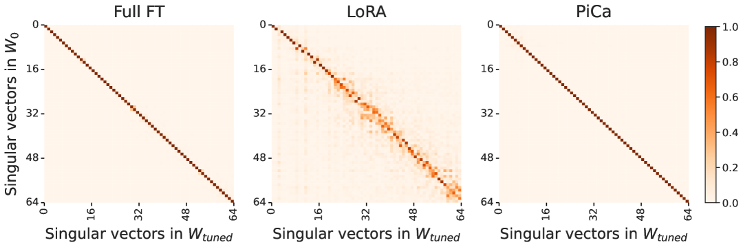
Figure 1: Spectral similarities between Full FT, LoRA, and PiCa in a representative example for DeBERTaV3_base. Color indicates the absolute cosine similarity between the singular vectors of pre-trained and fine-tuned weight matrices. Full FT and PiCa largely preserve spectral structure, whereas LoRA exhibits substantial deviation.

Though not explicitly motivated by these findings, recent PEFT methods have begun to exploit the spectral structure of pre-trained weights lingam2024svft ; meng2024pissa . One such example is Singular Vectors-guided Fine-Tuning (SVFT) lingam2024svft , which constructs a sparse, weighted combination of a model’s pre-trained singular vectors to achieve strong performance with fewer trainable parameters. Despite its empirical success, SVFT lacks a strong theoretical foundation for its reliance on pre-trained singular vectors. Moreover, it requires storing the full set of singular vectors during training, which leads to considerable memory overhead—an important drawback in the resource-constrained settings where PEFT is most critical (see Section 4.3 for experimental results).

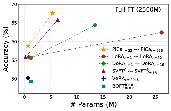
Figure 2: Average accuracy as a function of the number of trainable parameters on Commonsense Reasoning datasets using Gemma-2B. PiCa demonstrates superior performance compared to baseline methods with similar parameter budgets.

Derived from the spectral properties of fine-tuned weights in Fig. 1, we propose Parameter-efficient Fine-tuning with Column Space Projection (PiCa)–the first theoretically-grounded solution that leverages the column space of pre-trained weights spanned by their singular vectors. PiCa projects gradients onto the low rank column subspace based on principal singular vectors, exhibiting learning patterns close to Full FT. Unlike SVFT, our approach does not incur additional memory overhead from storing full singular vectors, making it significantly more practical in resource-constrained environments. Furthermore, we show that combining PiCa with weight sharing can significantly reduce the number of trainable parameters—surpassing even the most parameter-efficient configurations of other methods (e.g., rank-1 LoRA and DoRA). Our experiments across various models and datasets demonstrate that PiCa consistently outperforms baseline methods under comparable parameter budgets, as illustrated in Fig. 2.

Our contributions can be summarized as follows:

• We introduce PiCa, the first theoretically-grounded PEFT method based on the spectral properties of fine-tuned weights. PiCa projects gradients onto the low-rank column subspace of pre-trained weights, guided by their principal singular vectors, and exhibits learning patterns more closely aligned with Full FT.

• Extensive experiments demonstrate that PiCa achieves competitive or superior performance compared to existing PEFT methods. In particular, PiCa consistently outperforms the state-of-the-art baseline, SVFT, across all datasets and models, while SVFT incurs up to 25% extra memory overhead.

• We demonstrate that PiCa with weight sharing significantly reduces the number of trainable parameters up to 7$\times$ without compromising performance. This enables PiCa to achieve superior performance than LoRA using up to 13$\times$ fewer trainable parameters.

2 Related Work

Parameter-efficient fine-tuning

In adapting LLMs for downstream tasks, while Full FT often yields superior performance on these tasks, its substantial memory requirements have motivated the development of various PEFT methods that aim to achieve comparable performance with reduced computational overhead. Recently highlighted approaches include low rank approximation hu2022lora ; liu2024dora ; kopiczko2023vera , orthogonal reparametrization qiu2023controlling ; boft , and Singular Value Decomposition (SVD)-based approaches lingam2024svft ; meng2024pissa .

In particular, LoRA and its variants hu2022lora ; liu2024dora ; kopiczko2023vera have significant attention due to its simplicity and efficiency, based on approximating the update matrix $\Delta W$ using low-rank decomposition. However, recent studies suggest a performance gap compared to Full FT along with distinct learning behaviors. For instance, DoRA liu2024dora observes that LoRA exhibits a relatively high correlation between the magnitude and direction changes compared to Full FT. Moreover, Shuttleworth et al. shuttleworth2024lora highlights that there exists fundamentally different spectral characteristics between the outcomes of Full FT and LoRA.

On the other hand, methods leveraging the structure of pre-trained weights, specifically through their SVD components, have been explored lingam2024svft ; meng2024pissa . PiSSA meng2024pissa has reported that initializing the A and B matrices of LoRA using the SVD results of the pre-trained weights achieves better performance than standard LoRA. SVFT lingam2024svft utilizes the entire singular vectors of the pre-trained weights as a basis and employs a sparse matrix for updates. While SVFT achieves significant parameter reduction and better performance compared to LoRA, it requires substantial memory due to the need to store the entire singular vectors.

Although these SVD-based methods have shown empirical success, they often lack a strong theoretical foundation that provides an analytical justification for their methods. In contrast, we develop a method based on a theoretical proof that the optimal rank-$r$ approximation of $\Delta W$ can be achieved by the singular vectors of the pre-trained weights, which aligns with our empirical findings. We further validate this theoretical result through extensive experiments, demonstrating its effectiveness.

Weight sharing

Prior research has explored weight sharing to reduce the number of parameters in neural networks press-wolf-2017-using ; inan2016tying . More recently, this concept of weight sharing has been adapted within the LoRA framework kopiczko2023vera ; renduchintala2023tied ; zhou2025bishare ; shen2024sharelora ; song2024sharelora . For instance, VeRA kopiczko2023vera introduces a frozen random projection matrix shared across all layers, combined with trainable scaling vectors. Furthermore, recent works renduchintala2023tied ; song2024sharelora explore different strategies of combining freezing, training, and sharing both projection matrices and scaling vectors. While demonstrating progress in parameter reduction, these prior approaches tend to be highly sensitive to randomly initialized projection matrices and often their performance is below that of standard LoRA. However, in PiCa, we construct projection matrix based on structure of pre-trained weights for each layer and share trainable weights across layers with the same function role. This approach allows significant reduction of trainable parameters without performance degradation.

3 Methodology

Background

As first noted by shuttleworth2024lora and illustrated in Fig. 1, Full FT tends to preserve both the similarity of singular vectors and the ordering of their corresponding singular values between the pre-trained weight $W_{0}$ and the fine-tuned weight $W^{*}$. In contrast, LoRA fails to maintain this structure, resulting in a loss of spectral consistency. This observation suggests that the transformation from the singular vectors of $W_{0}$ to those of $W^{*}$ can be formalized as a structured perturbation of the form $I+E$, where $I$ is an identity matrix and $E$ is a matrix with small-magnitude entries.

Building on this insight, the following section demonstrates that the weight difference $\Delta W$ can be effectively approximated by projecting onto the principal column space of $W_{0}$. We provide theoretical justification for this claim and introduce PiCa, a method that leverages the spectral properties of pre-trained weights to more closely resemble the learning behavior of full fine-tuning within a low-rank adaptation framework, as shown in Fig. 1.

3.1 Parameter-Efficient Fine-Tuning with Column Space Projection (PiCa)

In this section, we present a mathematical justification of PiCa showing that projecting $\Delta W$ onto the top-$r$ principal components of the pre-trained weight matrix $W_{0}$ retains the essential directions of adaptation. The notations used in this paper are described in Appendix A. We begin by recalling a foundational result in low-rank approximation:

Lemma 3.1 (Eckart–Young Theorem eckart1936approximation ).

Let $A\in\mathbb{R}^{m\times n}$ have a Singular Value Decomposition (SVD) $A=U\Sigma V^{\top}$ with singular values $\sigma_{1}\geq\cdots\geq\sigma_{\min(m,n)}\geq 0$. The best rank-$r$ approximation $A_{r}=\sum_{i=1}^{r}\sigma_{i}u_{i}v_{i}^{\top}$ satisfies

$$A_{r}=\operatorname{argmin}_{\operatorname{rank}(B)\leq r}\|A-B\|_{F},$$

with minimum error $\|A-A_{r}\|_{F}^{2}=\sum_{i=r+1}^{\min(m,n)}\sigma_{i}^{2}$.

Based on the minimum error of the best rank-$r$ approximation provided by Lemma 3.1, we now derive an upper bound on the error incurred when projecting $\Delta W$ onto the column space spanned by the top-$r$ singular vectors of $W_{0}$:

Theorem 1.

Let $W_{0}=U\Sigma V^{\top}\in\mathbb{R}^{m\times n}$ be the Singular Value Decomposition (SVD) of $W_{0}$, where $\Sigma=\text{diag}(\sigma_{1}(W_{0}),\dots,\sigma_{\min(m,n)}(W_{0}))$. Suppose the fine-tuned matrix $W^{*}\in\mathbb{R}^{m\times n}$ has the form

$$W^{*}=(UP)\Sigma^{*}(VQ)^{\top},$$

where:

• $UP$ and $VQ$ are the left and right singular vectors of $W^{*}$, respectively.

• $\Sigma^{*}=\text{diag}(\sigma_{1}(W^{*}),\dots,\sigma_{\min(m,n)}(W^{*}))$,

• $P=I_{m}+E^{P}$ and $Q=I_{n}+E^{Q}$, with $|E^{P}_{ij}|<\epsilon$, $|E^{Q}_{ij}|<\epsilon$  for all $i,j$,

Let $\Delta W=W^{*}-W_{0}$, and let $U_{r}\in\mathbb{R}^{m\times r}$ be the top-$r$ left singular vectors of $W_{0}$. Then, the approximation error incurred by projecting $\Delta W$ onto the subspace spanned by $U_{r}$ is upper bounded as follows:

$$\left\|\Delta W-U_{r}U_{r}^{\top}\Delta W\right\|_{F}^{2}\leq\sum_{i=r+1}^{\min(m,n)}\sigma_{i}^{2}(\Delta W)+\mathcal{O}(\epsilon).$$

The complete proof of Theorem 1 is detailed in Appendix B.

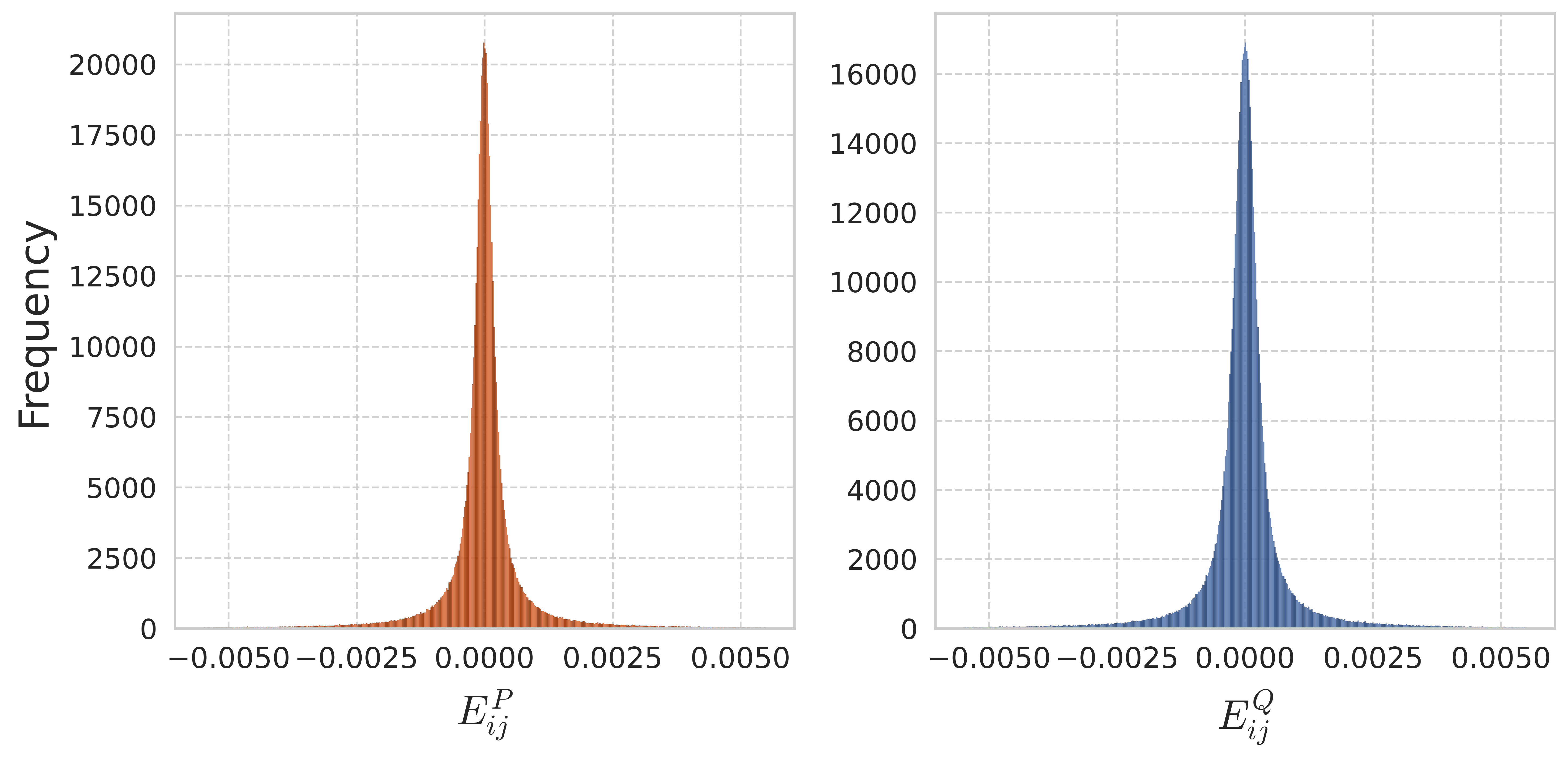
Figure 3: Distribution of perturbations $E_{ij}^{P}$ and $E_{ij}^{Q}$ across all weight matrix elements. Most values are tightly concentrated around zero, validating that $\mathcal{O}(\epsilon)$ is negligible in practice.

Theorem 1 shows that projecting the weight update onto the column space of the top singular vectors of $W_{0}$ yields a near-optimal low-rank approximation in Frobenius norm. The error is bounded by the residual singular values beyond rank $r$, plus a small perturbation due to the structured transformation. Empirical evidence in Fig. 3 using DeBERTaV3_base shows that the elements of perturbation matrices $E^{P}$ and $E^{Q}$ are highly concentrated near zero, indicating that the $\mathcal{O}(\epsilon)$ term is negligible in practice.

Formulation

Based on Theorem 1, we introduce PiCa, which leverages the low rank column subspace spanned by principal singular vectors. Let $W_{0}\in\mathbb{R}^{m\times n}$ denote a weight matrix from the pre-trained model. To enable efficient adaptation, we introduce a structured low-rank update $\Delta W$, guided by SVD of $W_{0}$:

$$W_{0}=U\Sigma V^{\top},$$

where $U\in\mathbb{R}^{m\times m}$ and $V\in\mathbb{R}^{n\times n}$ are orthogonal matrices containing the left and right singular vectors of $W_{0}$, and $\Sigma\in\mathbb{R}^{m\times n}$ is a diagonal matrix of singular values.

We construct $\Delta W$ using the top-$r$ left singular vectors of $W_{0}$, denoted by $U_{r}\in\mathbb{R}^{m\times r}$, as follows:

$$\Delta W=U_{r}B,$$

where $B\in\mathbb{R}^{r\times n}$ is a trainable matrix initialized with zero and $U_{r}$ remains fixed during fine-tuning. Then, the layer output under PiCa is given by:

$$Y=X(W_{0}+\Delta W)=X(W_{0}+U_{r}B),$$

where $X\in\mathbb{R}^{L\times m}$ is the input and $Y\in\mathbb{R}^{L\times n}$ is the output.

Column space projection of gradients

As presented in Table 1, PiCa can be interpreted through the lens of gradient projection. In Table 1, (1a)-(3a) illustrate the gradient update in full fine-tuning with fixed $W_{0}$, while (2a)-(2c) show the gradient update in PiCa. Notably, $U_{r}U_{r}^{\top}$ in (2c) represents the orthogonal projector onto the principal subspace spanned by the top-$r$ left singular vectors of the pre-trained weight matrix $W_{0}$. Comparing (2c) with (1c), we can observe that the PiCa update is equivalent to projecting the full fine-tuning gradient onto the column space formed by $U_{r}$. As the effective update of $\Delta W$ lies within this subspace, proved by Theorem 1, projecting gradients onto this subspace can be interpreted as restricting learning patterns to most informative directions with the greatest spectral significance, mitigating the effect of noisy or less relevant updates.

Table 1: Comparison of gradient update mechanisms in Full FT and PiCa

Full FT	PiCa
$\begin{array}[]{r@{\quad}l}\text{(1a)}&Y=X(W_{0}+\Delta W)\\ \text{(1b)}&\dfrac{\partial\mathcal{L}}{\partial(\Delta W)}=X^{\top}\dfrac{\partial\mathcal{L}}{\partial Y}\\ \text{(1c)}&\Delta W\leftarrow\Delta W-\eta\cdot X^{\top}\dfrac{\partial\mathcal{L}}{\partial Y}\end{array}$	$\begin{array}[]{r@{\quad}l}\text{(2a)}&Y=X(W_{0}+U_{r}B)\\ \text{(2b)}&\dfrac{\partial\mathcal{L}}{\partial B}=U_{r}^{\top}\left(X^{\top}\dfrac{\partial\mathcal{L}}{\partial Y}\right)\\ \text{(2c)}&\Delta W\leftarrow\Delta W-\eta\cdot U_{r}U_{r}^{\top}(X^{\top}\dfrac{\partial\mathcal{L}}{\partial Y})\end{array}$

3.2 Weight sharing

Although projecting updates onto the principal subspace already yields strong performance with significantly fewer trainable parameters compared to LoRA, we further enhance the efficiency of PiCa by incorporating weight sharing. Specifically, we share the $B$ matrices across layers that serve the same functional roles and have identical tensor shapes, expressed as:

$$\Delta W^{f,i}=U_{r}^{f,i}B^{f},\quad f\in\{\text{query,key,value,\ldots}\},\quad i\in\{1,2,\dots,L\},$$

where $f$ and $i$ represent the functional group and layer index, respectively; $\Delta W^{f,i}\in\mathbb{R}^{m\times n}$, $U_{r}^{f,i}\in\mathbb{R}^{m\times r}$, and $B^{f}\in\mathbb{R}^{r\times n}$. This strategy significantly reduces the number of trainable parameters, which allows for the use of higher ranks $r$ with minimal additional memory overhead.

Unlike prior approaches kopiczko2023vera ; renduchintala2023tied that primarily rely on random projection matrices for weight sharing, our method leverages layer-specific projection matrices $U_{r}^{f,i}$ derived from the structure of the pre-trained weights $W_{0}^{f,i}$ for each layer $i$ of group $f$. This allows us to capture the distinct characteristics and pretrained knowledge encoded in each $W_{0}^{f,i}$. Given the use of unique projection matrices per layer, we posit that the trainable matrix $B^{f}$ can be effectively shared across layers with the same functionality, facilitating efficient adaptation to downstream tasks.

Notably, using higher ranks $r$ not only increases the expressive capacity of the shared matrix $B^{f}$, but also enables the use of larger projection matrices $U_{r}^{f,i}$, resulting in more effective exploitation of pretrained knowledge through a greater number of singular vectors. Our extensive experiments demonstrate the effectiveness of weight sharing in PiCa, which reduces the number of trainable parameters by up to 7$\times$ without compromising performance (see Sec. 4.3 for details).

Table 2: Performance on Mathematical Reasoning benchmarks (GSM-8K and MATH). #Params indicates the number of trainable parameters. The best and second-best PEFT methods are highlighted in bold and underlined, respectively. For Gemma-7B, we set $r=16$ to ensure the number of trainable parameters remains below that of rank-1 LoRA. For SVFT${}_{d}^{R}$, we use $d=16$ for Gemma models and $d=12$ for LLaMA-3 models. In the high-rank setting, PiCa consistently achieves the best performance across all models and datasets, while using the fewest trainable parameters.

Method	Gemma-2B			Gemma-7B			LLaMA-3-8B
	#Params	GSM-8K	MATH	#Params	GSM-8K	MATH	#Params	GSM-8K	MATH
Full-FT	2.5B	52.69	17.94	8.5B	74.67	25.70	8.0B	64.13	16.24
$\text{BOFT}^{b=8}_{m=2}$	1.22M	36.01	12.13	2.90M	71.79	28.98	4.35M	67.09	21.64
$\text{DoRA}_{r=1}$	1.19M	35.35	13.04	3.26M	74.37	26.28	2.55M	68.30	21.96
$\text{LoRA}_{r=1}$	0.82M	32.97	13.04	0.82M	72.40	26.28	1.77M	68.84	20.94
$\text{VeRA}_{r=1024}$	0.63M	36.77	14.12	0.43M	71.11	27.04	0.98M	63.76	20.28
SVFTP	0.19M	40.34	14.38	0.43M	73.50	27.30	0.48M	69.22	20.44
PiCar=32	0.67M	41.32	15.22	0.64M	74.30	28.92	1.38M	73.54	24.14
$\text{LoRA}_{r=32}$	26.2M	43.06	15.50	68.8M	76.57	29.34	56.6M	75.89	24.74
$\text{DoRA}_{r=16}$	13.5M	44.27	16.18	35.5M	74.52	29.84	29.1M	75.66	24.72
SVFT${}^{R}_{\text{d}}$	6.35M	50.03	15.56	19.8M	76.81	29.98	13.1M	75.90	24.22
PiCar=256	5.37M	52.77	16.36	10.22M	78.39	30.16	11.01M	76.12	24.88

Table 3: Performance on Commonsense Reasoning benchmarks. #Params refers to the number of trainable parameters. The best and second-best PEFT methods are highlighted in bold and underlined text, respectively. In the high-rank setting, PiCa achieves state-of-the-art performance on 7 out of 8 datasets, using over 13$\times$ fewer parameters than LoRA and about half the parameters of SVFT.

Method	#Params	BoolQ	PIQA	SIQA	HS	WG	ARC-e	ARC-c	OBQA	Avg.
Full-FT	8.5B	72.32	87.32	76.86	91.07	81.76	92.46	82.87	89.00	84.19
DoRAr=1	3.31M	68.22	86.72	75.23	91.14	78.13	91.87	83.19	86.20	82.59
VeRAr=2048	1.49M	64.25	86.28	74.04	86.96	69.00	92.76	82.33	82.00	79.70
LoRAr=1	0.82M	65.44	86.28	75.02	89.91	75.92	91.79	81.91	85.40	81.46
SVFTP	0.51M	67.92	86.45	75.47	86.92	74.03	91.80	81.21	83.00	80.85
PiCar=16	0.64M	70.95	86.29	76.00	91.42	76.32	92.89	83.19	85.60	82.83
LoRAr=32	68.8M	71.55	87.95	77.27	91.80	79.71	92.67	82.16	86.40	83.69
DoRAr=16	35.5M	71.46	87.59	76.35	92.11	78.29	92.00	80.63	85.60	83.00
SVFT${}_{d=8}^{B}$	9.80M	71.90	86.96	76.28	91.55	78.76	92.80	83.11	85.40	83.35
PiCar=128	5.11M	72.84	87.98	77.79	92.82	79.40	93.14	83.62	88.20	84.47

Table 4: Performance of DeBERTaV3_base on the GLUE benchmark. #Params refers to the number of trainable parameters. The best and second-best PEFT methods are highlighted in bold and underlined text, respectively. While using more than 2.5$\times$ fewer parameters than $\text{SVFT}_{d=2}^{R}$, PiCa outperforms it on all datasets.

Method	#Params	MNLI	SST-2	MRPC	CoLA	QQP	QNLI	RTE	STS-B	Avg.
Full-FT	183.83M	89.90	95.63	89.46	69.19	92.40	94.03	83.75	91.60	88.25
$\text{LoRA}_{r=8}$	1.33M	90.65	94.95	89.95	69.82	93.87	91.99	85.20	91.60	88.50
$\text{LoRA}_{r=1}$	0.17M	90.12	95.64	86.43	69.13	91.43	94.18	87.36	91.52	88.23
$\text{DoRA}_{r=4}$	0.75M	89.92	95.41	89.10	69.37	91.53	94.14	87.00	91.80	88.53
$\text{BOFT}^{b=8}_{m=2}$	0.75M	90.25	96.44	92.40	72.95	92.10	94.23	88.81	91.92	89.89
$\text{VeRA}_{r=1024}$	0.09M	89.93	95.53	87.94	69.06	90.40	93.24	87.00	88.71	87.73
$\textsc{SVFT}^{P}$	0.06M	89.69	95.41	88.77	70.95	90.16	94.27	87.24	91.80	88.54
SVFT${}^{R}_{d=2}$	0.28M	89.97	95.99	88.99	72.61	91.50	93.90	88.09	91.73	89.10
PiCar=16	0.11M	90.20	96.00	91.40	73.10	91.60	94.20	89.20	91.80	89.69

4 Experiments

4.1 Experimental settings

We evaluate the effectivenss of PiCa across a diverse set of Natural Language Processing (NLP) tasks, covering Natural Language Generation (NLG), Commonsense Reasoning, and Natural Language Understanding (NLU). For NLG tasks, we fine-tune our model on the MetaMathQA-40K dataset yu2023metamath and assess its performance on the GSM-8K gsm8k and MATH hendrycks2021measuring datasets. Furthermore, we conduct evaluations on eight commonsense reasoning benchmarks: BoolQ boolq , PIQA piqa , SIQA socialiqa , HellaSwag hellaswag , Winogrande winogrande , ARC-Easy/ARC-Challenge arc , and OpenBookQA openbookqa . For NLU tasks, we utilize the GLUE benchmark glue . We report matched accuracy for MNLI, Matthew’s correlation for CoLA, Pearson correlation for STS-B, and accuracy for all other tasks. We employ the Gemma-2B/7B gemma , and LLaMA-3-8B llama3 models for NLG tasks and adopt the DeBERTaV3-base debertav3 model for NLU tasks. To ensure a fair comparison, hyperparameters and training protocols are aligned with those outlined in lingam2024svft . Unless explicitly mentioned, we use PiCa with weight sharing for all experiments. Further details are provided in the Appendix C.

4.2 Results

For a fair comparison, we follow lingam2024svft and evaluate the effectiveness of PiCa across three different tasks: NLG, Commonsense Reasoning, and NLU. The comparison baselines include LoRA hu2022lora , DoRA liu2024dora , BOFT boft , VeRA kopiczko2023vera , and SVFT lingam2024svft . All baseline results in Table 2, 3, and 4 are sourced from lingam2024svft .

Natural Language Generation

In Table 2, we provide results on mathematical question answering, comparing our method against baseline PEFT methods across three different base models ranging from 2B to 8B parameters. Our experiments include two configurations of PiCa: a high-rank setting with fewer trainable parameters than SVFT^R, and a low-rank configuration with fewer trainable parameters than rank 1 LoRA. As shown in Table 2, our high-rank PiCa consistently achieves superior performance while using the fewest trainable parameters across all models and datasets. In the low-rank setting, PiCa achieves either the best or second-best performance. Although SVFT^P uses fewer trainable parameters, it requires a substantially larger number of non-trainable parameters, resulting in higher GPU memory usage than our high-rank PiCa (see Section 4.3 for experimental results).

Commonsense Reasoning

In Table 3, we evaluate commonsense reasoning performance on eight benchmark datasets using Gemma-7B, following the same experimental setup as in the NLG task. We compare both high-rank and low-rank configurations of our method against PEFT baselines. In both settings, PiCa outperforms all baselines on average across the eight datasets. In the high-rank setting, our method achieves state-of-the-art performance on seven out of eight datasets while using over 13$\times$ fewer parameters than LoRA, and it consistently outperforms SVFT on all eight datasets with approximately half the number of parameters. In the low-rank setting, PiCa also achieves the best average performance, surpassing rank 1 DoRA while using more than 5$\times$ fewer parameters. Compared to SVFT^P, our method delivers superior performance on seven out of eight datasets, with an average improvement of nearly two percentage points. Similar trends are observed with Gemma-2B (see Appendix C.2).

Natural Language Understanding

Table 4 presents the results on the GLUE benchmark using DeBERTaV3_base. Compared to LoRA with rank 8, our method achieves over one percentage point higher average performance. While using more than 2.5$\times$ fewer parameters than SVFT${}_{d=2}^{R}$, our method outperforms it on all datasets. Furthermore, despite using over 7$\times$ fewer parameters than BOFT, our method achieves comparable average performance.

Table 5: Comparison of additional parameters and training memory for different methods on Gemma-2B. Training memory denotes the peak GPU memory usage during fine-tuning. Due to the presence of additional non-trainable parameters, SVFT requires up to 25% more memory than PiCa, even when it has fewer trainable parameters.

Method	Additional Params		Training Memory	Performance
	#Trainable	#Non-trainable		GSM-8K	MATH
SVFTP	0.19M	380.04M	20.23GB	40.34	14.38
SVFT${}^{R}_{d=16}$	6.35M	380.04M	20.68GB	50.03	15.57
PiCar=256	5.37M	113.25M	16.73GB	52.77	16.36

4.3 Further analysis

Analysis of memory consumption during fine-tuning

In this section, we present a comparative analysis of training memory usage between PiCa and the state-of-the-art baseline, SVFT. Training memory is measured with peak GPU memory usage during fine-tuning. As shown in Table 5, although both SVFT^P and SVFT${}^{R}_{d=16}$ significantly reduce the number of trainable parameters, they require over 380M additional non-trainable parameters that must be stored during fine-tuning and consume up to 25% more GPU memory than PiCa_r=256. This overhead stems from SVFT’s factorization of weight updates as $\Delta W=UMV^{\top}$, where $U\in\mathbb{R}^{m\times m}$ and $V\in\mathbb{R}^{n\times n}$ are the singular vectors of the pre-trained weight matrix $W_{0}\in\mathbb{R}^{m\times n}$. Although $U$ and $V$ remain non-trainable, SVFT must retain them throughout fine-tuning, incurring substantial memory costs. This comparison demonstrates that PiCa offers a more efficient solution, particularly in resource-constrained environments where memory I/O remains a critical bottleneck.

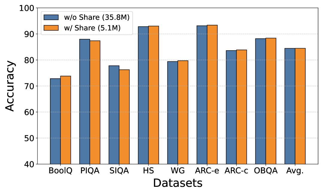
(a) Accuracy across Commonsense Reasoning datasets with and without weight sharing. Weight sharing reduces the number of trainable parameters by up to 7× without compromising performance.

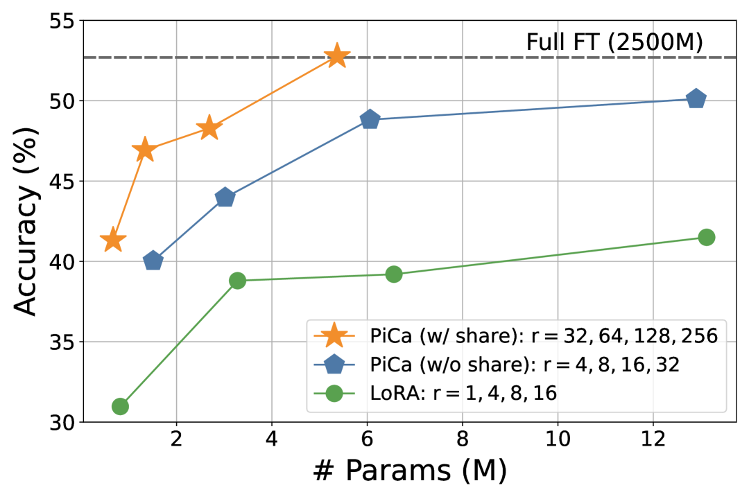
(b) Accuracy on GSM-8K under varying rank settings. Weight sharing consistently yields superior performance under similar parameter budgets.

Figure 4: Ablation study of weight sharing across different datasets and rank configurations.

Ablation study of weight sharing

In Fig. 4(a), we analyze the impact of weight sharing in PiCa across eight Commonsense Reasoning datasets using Gemma-7B. We compare two configurations: PiCa with rank 16 and no weight sharing (35.8M trainable parameters) and PiCa with rank 128 and weight sharing (5.1M trainable parameters). The results show that PiCa with weight sharing consistently achieves performance comparable to its ablation without sharing. This demonstrates that incorporating weight sharing into PiCa can reduce the number of trainable parameters by approximately 7$\times$ without degrading performance.

Furthermore, we conduct an additional study on the effect of weight sharing under varying rank settings using the GSM-8K benchmark with Gemma-2B. As shown in Fig. 4(b), PiCa consistently outperforms LoRA at comparable parameter budgets, regardless of whether weight sharing is applied. Notably, PiCa with rank 32 and weight sharing matches the performance of LoRA with rank 16, while requiring a similar number of trainable parameters comparable as rank 1 LoRA. Moreover, increasing the rank to 256 enables PiCa to reach the performance of Full FT, while still using fewer parameters than LoRA with rank 8. These results underscore the effectiveness of weight sharing in PiCa, which consistently achieves superior performance under similar parameter budgets compared to both LoRA and its no-sharing ablation.

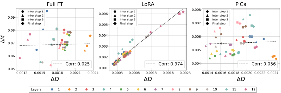
Figure 5: Analysis of the magnitude and directional updates of weight matrices in (a) Full FT, (b) LoRA, and (c) PiCa across different layers and training steps. Different markers denote training steps, while colors indicate different layers. LoRA shows a strong positive correlation between $\Delta D$ and $\Delta W$, whereas Full FT and PiCa exhibit similar learning patterns with negligible correlation.

Analysis of magnitude and direction updates

Following liu2024dora , we analyze changes in weight magnitude and direction during fine-tuning using DeBERTaV3${}_{\text{base}}$. We decompose the weight matrix $W\in\mathbb{R}^{d\times k}$ as $W=mV/||V||_{c}$, where $m\in\mathbb{R}^{1\times k}$ is the magnitude vector, $V\in\mathbb{R}^{d\times k}$ is the directional matrix, and $||\cdot||_{c}$ is the column-wise norm. We compute the magnitude change as $\Delta M=\sum_{n=1}^{k}|m_{\text{tuned}}^{n}-m_{0}^{n}|/{k}$ and the directional change as $\Delta D=\sum_{n=1}^{k}(1-\mathbf{cos}(V_{\text{tuned}}^{n},W_{0}^{n}))/{k}$, measuring the differences between pre-trained and fine-tuned weights.

We fine-tune all layers and evaluate these metrics across four training checkpoints for all layers of the query matrix under Full FT, LoRA, and PiCa. Consistent with the findings of liu2024dora , we observe that Full FT and LoRA exhibit distinct learning patterns in both magnitude and direction, as illustrated in Fig. 5. In particular, LoRA shows a positive correlation between $\Delta D$ and $\Delta W$ with a value of 0.974, whereas Full FT displays more varied learning pattern with negligible correlation with a value of 0.025. While PiCa is designed to align with Full FT in terms of spectral properties, our analysis in Fig. 5 shows that it also closely matches Full FT in directional and magnitude update patterns.

5 Discussion

While PiCa shares the same goal as LoRA in enabling efficient adaptation, it introduces a minor limitation during inference. Specifically, LoRA requires loading the stored weight matrices $A$ and $B$, computing their product, and adding the result to the pretrained weights. In contrast, PiCa stores only a much smaller shared matrix $B$, but must perform an additional SVD on the pretrained weights $W_{0}$ at load time to recover the projection matrix $A$. This presents a trade-off between storage cost and computational overhead during model initialization. If the initialization overhead is a concern, one can optionally store $A$, as in LoRA. Nonetheless, in scenarios where multiple task-specific adaptations are required from a single base model, PiCa offers greater scalability: a shared set of task-agnostic $A$ matrices can be precomputed and paired with multiple sets of lightweight task-specific $B$ matrices, enabling efficient adaptation across diverse tasks.

6 Conclusion

In this work, we introduce PiCa, a theoretically grounded PEFT method that projects gradients onto the low-rank column subspace of pre-trained weights, preserving their spectral structure and aligning more closely with Full FT. Unlike SVFT, PiCa avoids the memory overhead of storing full singular vectors and, when combined with weight sharing, significantly reduces the number of trainable parameters without compromising performance. Extensive experiments across diverse datasets and models demonstrate that PiCa achieves superior or competitive performance compared to existing PEFT methods. In future work, we aim to extend PiCa to more dynamic and practical settings such as multi-task adaptation and continual learning, where efficient and scalable fine-tuning is critical.

Appendix

Appendix A Preliminaries

A.1 Notation

Notation 1.

The following notation is used throughout this paper:

• For any matrix $A\in\mathbb{R}^{m\times n}$, let $\sigma_{i}(A)$ denote its $i$-th largest singular value, with $\sigma_{1}(A)\geq\sigma_{2}(A)\geq\cdots\geq\sigma_{\min(m,n)}(A)\geq 0$.

• $\|A\|_{F}$: Frobenius norm of matrix $A$, defined as $\|A\|_{F}=\sqrt{\sum_{i,j}A_{ij}^{2}}$.

• $\|A\|_{2}$: Spectral norm of matrix $A$, defined as $\|A\|_{2}=\sigma_{1}(A)$.

• $A_{ij}$: Entry at the $i$-th row and $j$-th column of matrix $A$.

• $I_{k}$: Identity matrix of size $k\times k$.

• $\text{diag}(a_{1},\dots,a_{n})$: Diagonal matrix with entries $a_{1},\dots,a_{n}$.

A.2 Preliminary Results

Lemma A.1 (Weyl’s Inequality for Singular Values weyl1912asymptotische ).

Let $A,B\in\mathbb{R}^{m\times n}$. Then, for all $i=1,\dots,\min(m,n)$:

$$|\sigma_{i}(A+B)-\sigma_{i}(A)|\leq\|B\|_{2}.$$

Lemma A.2 (Invariance of Frobenius Norm under Orthogonal Transformations).

Let $A\in\mathbb{R}^{m\times n}$, and let $U\in\mathbb{R}^{m\times m}$ and $V\in\mathbb{R}^{n\times n}$ be orthogonal matrices. Then:

$$\|UAV^{T}\|_{F}=\|A\|_{F}.$$

Appendix B Proof of Theorem

Theorem 1.

Let $W=U\Sigma V^{\top}\in\mathbb{R}^{m\times n}$ be the Singular Value Decomposition (SVD) of $W$, where $\Sigma=\text{diag}(\sigma_{1}(W),\dots,\sigma_{\min(m,n)}(W))$. Suppose the fine-tuned matrix $W^{*}\in\mathbb{R}^{m\times n}$ has the form

$$W^{*}=(UP)\Sigma^{*}(VQ)^{\top},$$

where:

• $UP$ and $VQ$ are the left and right singular vectors of $W^{*}$, respectively.

• $\Sigma^{*}=\text{diag}(\sigma_{1}(W^{*}),\dots,\sigma_{\min(m,n)}(W^{*}))$,

• $P=I_{m}+E^{P}$ and $Q=I_{n}+E^{Q}$, with $|E^{P}_{ij}|<\epsilon$, $|E^{Q}_{ij}|<\epsilon$  for all $i,j$,

Let $\Delta W=W^{*}-W$, and let $U_{r}\in\mathbb{R}^{m\times r}$ be the top-$r$ left singular vectors of $W$. Then, the approximation error incurred by projecting $\Delta W$ onto the subspace spanned by $U_{r}$ is upper bounded as follows:

$$\left\|\Delta W-U_{r}U_{r}^{\top}\Delta W\right\|_{F}^{2}\leq\sum_{i=r+1}^{\min(m,n)}\sigma_{i}^{2}(\Delta W)+\mathcal{O}(\epsilon).$$

Proof.

We derive the inequality through a series of steps, decomposing the perturbation, analyzing the projection error, and bounding the terms using spectral and entrywise techniques.

B.1 Decompose the Perturbation

The perturbed matrix is:

$$W^{*}=U(I_{m}+E^{P})\Sigma^{*}(I_{n}+E^{Q})^{\top}V^{\top}.$$

The perturbation is:

$$\Delta W=W^{*}-W=U\left[(I_{m}+E^{P})\Sigma^{*}(I_{n}+E^{Q})^{\top}-\Sigma\right]V^{\top}.$$

Define:

$$H=(I_{m}+E^{P})\Sigma^{*}(I_{n}+E^{Q})^{\top}-\Sigma,$$

so:

$$\Delta W=UHV^{\top}.$$

Expand:

$$(I_{m}+E^{P})\Sigma^{*}(I_{n}+E^{Q})^{\top}=\Sigma^{*}+E^{P}\Sigma^{*}+\Sigma^{*}(E^{Q})^{\top}+E^{P}\Sigma^{*}(E^{Q})^{\top}.$$

Thus:

$$H=\Sigma^{*}-\Sigma+E^{P}\Sigma^{*}+\Sigma^{*}(E^{Q})^{\top}+E^{P}\Sigma^{*}(E^{Q})^{\top}.$$

Let:

$$D=\Sigma^{*}-\Sigma,\quad E_{1}=E^{P}\Sigma^{*},\quad E_{2}=\Sigma^{*}(E^{Q})^{\top},\quad E_{3}=E^{P}\Sigma^{*}(E^{Q})^{\top}.$$

So:

$$H=D+E_{1}+E_{2}+E_{3}.$$

The matrix $D$ is diagonal:

$$D_{ii}=\sigma_{i}(W^{*})-\sigma_{i}(W)\quad\text{for }i\leq\min(m,n),\quad D_{ij}=0\text{ if }i\neq j.$$

B.2 Projection Error Analysis

The projection error is:

$$\|\Delta W-U_{r}U_{r}^{\top}\Delta W\|_{F}^{2}.$$

Since $\Delta W=UHV^{\top}$, and $U_{r}^{\top}U=[I_{r}\;0]$, we have:

$$U_{r}U_{r}^{\top}\Delta W=U\begin{bmatrix}I_{r}&0\\ 0&0\end{bmatrix}HV^{\top}.$$

Thus:

$$\Delta W-U_{r}U_{r}^{\top}\Delta W=U\left(H-\begin{bmatrix}I_{r}&0\\ 0&0\end{bmatrix}H\right)V^{\top}.$$

Define:

$$P_{r}=\begin{bmatrix}I_{r}&0\\ 0&0\end{bmatrix}.$$

By Lemma A.2, frobenius norm is:

$$\|\Delta W-U_{r}U_{r}^{\top}\Delta W\|_{F}^{2}=\|H-P_{r}H\|_{F}^{2}=\sum_{i=r+1}^{m}\sum_{j=1}^{n}H_{ij}^{2}.$$

B.3 Entry-wise bounds

For $i>r$, compute $H_{ij}$:

$$H_{ij}=D_{ij}+E_{1,ij}+E_{2,ij}+E_{3,ij}.$$

B.3.1 Diagonal Terms ($j=i$)

$$H_{ii}=\sigma_{i}(W^{*})-\sigma_{i}(W)+E^{P}_{ii}\sigma_{i}(W^{*})+\sigma_{i}(W^{*})E^{Q}_{ii}+\sum_{k=1}^{\min(m,n)}E^{P}_{ik}\sigma_{k}(W^{*})E^{Q}_{ik}.$$

Define:

$$D_{ii}=\sigma_{i}(W^{*})-\sigma_{i}(W),\quad E_{1,ii}=E^{P}_{ii}\sigma_{i}(W^{*})$$

$$E_{2,ii}=\sigma_{i}(W^{*})E^{Q}_{ii},\quad E_{3,ii}=\sum_{k=1}^{\min(m,n)}E^{P}_{ik}\sigma_{k}(W^{*})E^{Q}_{ik}.$$

Bound using $|E^{P}_{ij}|<\epsilon$, $|E^{Q}_{ij}|<\epsilon$:

$$|E_{1,ii}|\leq\epsilon\sigma_{i}(W^{*}),$$

$$|E_{2,ii}|\leq\epsilon\sigma_{i}(W^{*}),$$

$$|E_{3,ii}|\leq\epsilon^{2}\sum_{k=1}^{\min(m,n)}\sigma_{k}(W^{*})\leq\epsilon^{2}{\min(m,n)}\sigma_{\max}(W^{*}).$$

B.3.2 Off-Diagonal Terms ($j\neq i$)

$$H_{ij}=E^{P}_{ij}\sigma_{j}(W^{*})+\sigma_{i}(W^{*})E^{Q}_{ji}+\sum_{k=1}^{\min(m,n)}E^{P}_{ik}\sigma_{k}(W^{*})E^{Q}_{jk}.$$

Define:

$$E_{1,ij}=E^{P}_{ij}\sigma_{j}(W^{*}),\quad E_{2,ij}=\sigma_{i}(W^{*})E^{Q}_{ji},\quad E_{3,ij}=\sum_{k=1}^{\min(m,n)}E^{P}_{ik}\sigma_{k}(W^{*})E^{Q}_{jk}.$$

Bound:

$$|E_{1,ij}|\leq\epsilon\sigma_{j}(W^{*}),$$

$$|E_{2,ij}|\leq\epsilon\sigma_{i}(W^{*}),$$

$$|E_{3,ij}|\leq\epsilon^{2}\min(m,n)\sigma_{\max}(W^{*}).$$

B.4 Sum Squared Entries

The projection error is:

$$\sum_{i=r+1}^{m}\sum_{j=1}^{n}H_{ij}^{2}=\sum_{i=r+1}^{\min(m,n)}H_{ii}^{2}+\sum_{i=r+1}^{m}\sum_{\begin{subarray}{c}j=1\\ j\neq i\end{subarray}}^{n}H_{ij}^{2}.$$

For diagonal terms:

$$H_{ii}^{2}=(\sigma_{i}(W^{*})-\sigma_{i}(W))^{2}+2(\sigma_{i}(W^{*})-\sigma_{i}(W))(E_{1,ii}+E_{2,ii}+E_{3,ii})+(E_{1,ii}+E_{2,ii}+E_{3,ii})^{2}.$$

Bound the cross term:

$$2(\sigma_{i}(W^{*})-\sigma_{i}(W))(E_{1,ii}+E_{2,ii}+E_{3,ii})\leq 2|\sigma_{i}(W^{*})-\sigma_{i}(W)|(|E_{1,ii}|+|E_{2,ii}|+|E_{3,ii}|).$$

The quadratic term:

$$(E_{1,ii}+E_{2,ii}+E_{3,ii})^{2}\leq 3(E_{1,ii}^{2}+E_{2,ii}^{2}+E_{3,ii}^{2}).$$

Sum:

$$\sum_{i=r+1}^{\min(m,n)}H_{ii}^{2}\leq\sum_{i=r+1}^{\min(m,n)}(\sigma_{i}(W^{*})-\sigma_{i}(W))^{2}+\epsilon C_{1}+\epsilon^{2}C_{2}.$$

Where:

$$C_{1}=\sum_{i=r+1}^{\min(m,n)}2|\sigma_{i}(W^{*})-\sigma_{i}(W)|(2\sigma_{i}(W^{*})+\epsilon\min(m,n)\sigma_{max}(W^{*}))$$

$$C_{2}=\sum_{i=r+1}^{\min(m,n)}3(2\sigma_{i}^{2}(W^{*})+\epsilon^{2}\min(m^{2},n^{2})\sigma_{max}^{2}(W^{*})\$$

For off-diagonal terms:

$$\sum_{i=r+1}^{m}\sum_{\begin{subarray}{c}j=1\\ j\neq i\end{subarray}}^{n}H_{ij}^{2}=\sum_{i=r+1}^{m}\sum_{\begin{subarray}{c}j=1\\ j\neq i\end{subarray}}^{n}(E_{1,ij}+E_{2,ij}+E_{3,ij})^{2}\leq\sum_{i=r+1}^{m}\sum_{\begin{subarray}{c}j=1\\ j\neq i\end{subarray}}^{n}3(E_{1,ij}^{2}+E_{2,ij}^{2}+E_{3,ij}^{2})\leq\epsilon^{2}C_{3}.$$

Where:

$$C_{3}=\sum_{i=r+1}^{m}\sum_{\begin{subarray}{c}j=1\\ j\neq i\end{subarray}}^{n}3(\sigma_{j}^{2}(W^{*})+\sigma_{i}^{2}(W^{*})+\epsilon^{2}\min(m^{2},n^{2})\sigma_{max}^{2}(W^{*}))$$

Therefore:

$$\sum_{i=r+1}^{m}\sum_{j=1}^{n}H_{ij}^{2}\leq\sum_{i=r+1}^{\min(m,n)}(\sigma_{i}(W^{*})-\sigma_{i}(W))^{2}+\epsilon C_{1}+\epsilon^{2}C_{2}+\epsilon^{2}C_{3}$$

B.5 Spectral Norm Bounds

Recall:

$$H=D+E_{1}+E_{2}+E_{3}.$$

By Lemma A.2:

$$\sigma_{i}(\Delta W)=\sigma_{i}(H)$$

Since $UP$ and $VQ$ are singular vectors of $W^{*}$, $P$ and $Q$ are orthogonal matrices. Therefore:

$$\sigma_{i}(D)=|\sigma_{i}(\Sigma^{*})-\sigma_{i}(\Sigma)|=|\sigma_{i}(W^{*})-\sigma_{i}(W)|,\ \forall i$$

By Lemma A.1:

$$|\sigma_{i}(H)-\sigma_{i}(D)|=|\sigma_{i}(\Delta W)-|\sigma_{i}(W*)-\sigma_{i}(W)||\leq\|E_{1}+E_{2}+E_{3}\|_{2}=\|E_{total}\|$$

Bound:

$$\|E_{1}\|_{2}\leq\|E^{P}\|_{2}\sigma_{\max}(W^{*})\leq\|E^{P}\|_{F}\sigma_{\max}(W^{*})\leq\sqrt{mn}\epsilon\sigma_{\max}(W^{*}),$$

$$\|E_{2}\|_{2}\leq\sqrt{mn}\epsilon\sigma_{\max}(W^{*}),$$

$$\|E_{3}\|_{2}\leq mn\epsilon^{2}\sigma_{\max}(W^{*}).$$

Thus:

$$\|E_{total}\|_{2}\leq 2\sqrt{mn}\epsilon\sigma_{\max}(W^{*})+mn\epsilon^{2}\sigma_{\max}(W^{*}).$$

To bound $\sum_{i=r+1}^{\min(m,n)}(\sigma_{i}(W^{*})-\sigma_{i}(W))^{2}$, we express $\sigma_{i}(W^{*})-\sigma_{i}(W)$ in terms of $\sigma_{i}(\Delta W)$.

Consider the identity:

$$|\sigma_{i}(W^{*})-\sigma_{i}(W)|=\sigma_{i}(\Delta W)-(\sigma_{i}(\Delta W)-|\sigma_{i}(W^{*})-\sigma_{i}(W)|).$$

Let:

$$\delta_{i}=\sigma_{i}(\Delta W)-|\sigma_{i}(W^{*})-\sigma_{i}(W)|,$$

Then

$$|\sigma_{i}(W^{*})-\sigma_{i}(W)|=\sigma_{i}(\Delta W)-\delta_{i}.$$

where

$$|\delta_{i}|\leq\|E_{\text{total}}\|_{2}$$

Square both sides:

$$(\sigma_{i}(W^{*})-\sigma_{i}(W))^{2}=(\sigma_{i}(\Delta W)-\delta_{i})^{2}=\sigma_{i}^{2}(\Delta W)-2\sigma_{i}(\Delta W)\delta_{i}+\delta_{i}^{2}.$$

Since $|\delta_{i}|\leq\|E_{\text{total}}\|_{2}$, we bound the terms:

• Cross term: $|2\sigma_{i}(\Delta W)\delta_{i}|\leq 2\sigma_{i}(\Delta W)\|E_{\text{total}}\|_{2}$

• Quadratic term: $\delta_{i}^{2}\leq\|E_{\text{total}}\|_{2}^{2}$.

Thus:

$$(\sigma_{i}(W^{*})-\sigma_{i}(W))^{2}\leq\sigma_{i}^{2}(\Delta W)+2\sigma_{i}(\Delta W)\|E_{\text{total}}\|_{2}+\|E_{\text{total}}\|_{2}^{2}.$$

Summing over $i=r+1$ to $\min(m,n)$:

$$\sum_{i=r+1}^{\min(m,n)}(\sigma_{i}(W^{*})-\sigma_{i}(W))^{2}\leq \sum_{i=r+1}^{\min(m,n)}\sigma_{i}^{2}(\Delta W)+2\|E_{\text{total}}\|_{2}\sum_{i=r+1}^{\min(m,n)}\sigma_{i}(\Delta W)$$

$$+ (\min(m,n)-r)\|E_{\text{total}}\|_{2}^{2}.$$

Therefore:

$$\sum_{i=r+1}^{\min(m,n)}(\sigma_{i}(W^{*})-\sigma_{i}(W))^{2}\leq\sum_{i=r+1}^{\min(m,n)}\sigma_{i}^{2}(\Delta W)+\epsilon C_{4}+\epsilon^{2}C_{5}.$$

Where:

$$C_{4}=2(2\sqrt{mn}\sigma_{\max}(W^{*})+mn\epsilon\sigma_{\max}(W^{*}))\sum_{i=r+1}^{\min(m,n)}\sigma_{i}(\Delta W)$$

$$C_{5}=(\min(m,n)-r)(2\sqrt{mn}\sigma_{\max}(W^{*})+mn\epsilon\sigma_{\max}(W^{*}))^{2}$$

Combine:

$$\|\Delta W-U_{r}U_{r}^{\top}\Delta W\|_{F}^{2}\leq \sum_{i=r+1}^{\min(m,n)}\sigma_{i}^{2}(\Delta W)+\epsilon C_{1}+\epsilon^{2}C_{2}+\epsilon^{2}C_{3}+\epsilon C_{4}+\epsilon^{2}C_{5}$$

$$= \sum_{i=r+1}^{\min(m,n)}\sigma_{i}^{2}(\Delta W)+\epsilon C$$

where:

$$C=(C_{1}+\epsilon C_{2}+\epsilon C_{3}+C_{4}+\epsilon C_{5})$$

∎

Appendix C Implementation Details and Additional Experiments

To ensure a direct and unbiased comparison with existing baseline methods, we adopted the same experimental setup as outlined in SVFT lingam2024svft . For consistency, all baseline results were also sourced from lingam2024svft , enabling a fair evaluation of our method’s performance.

C.1 Implementation Details

Natural Language Generation

Table 6 presents the hyperparameter configurations employed for these experiments. For the Gemma model family, PiCa is applied to the $Q,K,V,U,D$ matrices, while for the LLaMA-3-8B model, the $Q,K,V,U,D,O,G$ matrices are targeted. The experimental codebase and evaluation procedures are adapted from https://github.com/VijayLingam95/SVFT.git, and the fine-tuning dataset are sourced from https://huggingface.co/datasets/meta-math/MetaMathQA-40K.

Table 6: Hyperparameter setup used for fine-tuning on MetaMathQA-40K.

Hyperparameter	Gemma-2B		Gemma-7B		LLaMA-3-8B
Optimizer	AdamW
Warmup Ratio	0.1
LR Schedule	Cosine
Max Seq. Len.	512
# Epochs	2
Batch Size	64
Rank	32	256	16	256	32	256
Learning Rate	1E-03	9E-04	1E-04	5E-05	2E-04	2E-04

Commonsense Reasoning

We follow the setting outlined in prior work lingam2024svft , fine-tuning on 15K examples. The hyperparameter configurations for these experiments are detailed in  Table 7. We utilize the same set of matrices as in the natural language generation tasks. The codebase, including training and evaluation data, is sourced from https://github.com/VijayLingam95/SVFT.git.

Table 7: Hyperparameter setup used for fine-tuning on commonsense-15K.

Hyperparameter	Gemma-2B		Gemma-7B
Optimizer	AdamW
Warmup Steps	100
LR Schedule	Linear
Max Seq. Len.	512
# Epochs	3
Batch Size	64
Rank	32	256	16	128
Learning Rate	1E-03	9E-04	3E-04	8E-05

Natural Language Understanding

We fine-tune DeBERTaV3_base debertav3 , applying PiCa to all linear layers within each transformer block. We constrain hyperparameter optimization to moderate adjustments of the learning rate and the number of training epochs. For rigorous comparison, we employ identical model sequence lengths to those reported by lingam2024svft ; boft . The precise hyperparameter settings utilized in these experiments are specified in Table 8.

Table 8: Hyperparameter setup used for DeBERTaV3_base on the GLUE benchmark.

Method	Dataset	MNLI	SST-2	MRPC	CoLA	QNLI	QQP	RTE	STS-B
	Optimizer	AdamW
	Warmup Ratio	0.1
	LR Schedule	Linear
	Batch Size	32
	Max Seq. Len.	256	128	320	64	512	320	320	128
PiCar=16	Learning Rate	3E-04	1E-03	2E-03	8E-4	3E-04	1E-04	1E-03	3E-03
	# Epochs	5	7	35	50	5	15	40	15

C.2 Commonsense Reasoning with Gemma-2B

We evaluate PiCa on commonsense reasoning tasks with Gemma-2B. The results are presented in Table 9. PiCa achieves the highest average performance across both high- and low-rank settings, outperforming the second-best method by approximately 2–3 percentage points.

Table 9: Performance on Commonsense Reasoning benchmarks using Gemma-2B. #Params refers to the number of trainable parameters. The best and second-best PEFT methods are highlighted in bold and underlined text, respectively. PiCa achieves state-of-the-art average performance across both high- and low-rank settings, outperforming the second-best method by up to 3 percentage points.

Method	#Params	BoolQ	PIQA	SIQA	HS	WG	ARC-e	ARC-c	OBQA	Avg.
Full-FT	2.5B	63.57	74.10	65.86	70.00	61.95	75.36	59.72	69.00	67.45
$\text{BOFT}^{b=8}_{m=2}$	1.22M	59.23	63.65	47.90	29.93	50.35	59.04	42.66	41.00	49.22
VeRAr=2048	0.66M	62.11	64.31	49.18	32.00	50.74	58.08	42.83	42.60	50.23
LoRAr=1	0.82M	62.20	69.31	56.24	32.47	51.53	69.52	48.80	56.40	55.81
DoRAr=1	1.19M	62.17	68.77	55.93	32.95	51.22	68.81	48.72	55.60	55.52
SVFTP	0.19M	62.26	70.18	56.70	32.47	47.04	69.31	50.08	58.40	55.81
PiCar=32	0.67M	62.11	71.76	60.13	36.49	50.59	73.74	52.56	63.20	58.82
LoRAr=32	26.2M	63.11	73.44	63.20	47.79	52.95	74.78	57.16	67.00	62.43
DoRAr=16	13.5M	62.87	73.93	65.34	53.16	55.51	76.43	59.55	68.40	64.40
SVFT${}_{B}^{d=16}$	6.35M	63.42	73.72	63.86	71.21	59.58	73.69	54.77	66.60	65.86
PiCa r=256	5.37M	63.91	75.57	64.38	71.75	60.62	77.44	58.70	68.40	67.60

References

- [1] Neil Houlsby, Andrei Giurgiu, Stanislaw Jastrzebski, Bruna Morrone, Quentin De Laroussilhe, Andrea Gesmundo, Mona Attariyan, and Sylvain Gelly. Parameter-efficient transfer learning for nlp. In International conference on machine learning, pages 2790–2799. PMLR, 2019.
- [2] Edward J Hu, Yelong Shen, Phillip Wallis, Zeyuan Allen-Zhu, Yuanzhi Li, Shean Wang, Lu Wang, Weizhu Chen, et al. Lora: Low-rank adaptation of large language models. ICLR, 1(2):3, 2022.
- [3] Reece Shuttleworth, Jacob Andreas, Antonio Torralba, and Pratyusha Sharma. Lora vs full fine-tuning: An illusion of equivalence. arXiv preprint arXiv:2410.21228, 2024.
- [4] Shih-Yang Liu, Chien-Yi Wang, Hongxu Yin, Pavlo Molchanov, Yu-Chiang Frank Wang, Kwang-Ting Cheng, and Min-Hung Chen. Dora: Weight-decomposed low-rank adaptation. In Forty-first International Conference on Machine Learning, 2024.
- [5] Vijay Chandra Lingam, Atula Neerkaje, Aditya Vavre, Aneesh Shetty, Gautham Krishna Gudur, Joydeep Ghosh, Eunsol Choi, Alex Dimakis, Aleksandar Bojchevski, and Sujay Sanghavi. Svft: Parameter-efficient fine-tuning with singular vectors. Advances in Neural Information Processing Systems, 37:41425–41446, 2024.
- [6] Fanxu Meng, Zhaohui Wang, and Muhan Zhang. Pissa: Principal singular values and singular vectors adaptation of large language models. Advances in Neural Information Processing Systems, 37:121038–121072, 2024.
- [7] Dawid J Kopiczko, Tijmen Blankevoort, and Yuki M Asano. Vera: Vector-based random matrix adaptation. arXiv preprint arXiv:2310.11454, 2023.
- [8] Zeju Qiu, Weiyang Liu, Haiwen Feng, Yuxuan Xue, Yao Feng, Zhen Liu, Dan Zhang, Adrian Weller, and Bernhard Schölkopf. Controlling text-to-image diffusion by orthogonal finetuning. Advances in Neural Information Processing Systems, 36:79320–79362, 2023.
- [9] Weiyang Liu, Zeju Qiu, Yao Feng, Yuliang Xiu, Yuxuan Xue, Longhui Yu, Haiwen Feng, Zhen Liu, Juyeon Heo, Songyou Peng, Yandong Wen, Michael J. Black, Adrian Weller, and Bernhard Schölkopf. Parameter-efficient orthogonal finetuning via butterfly factorization. In The Twelfth International Conference on Learning Representations, 2024.
- [10] Ofir Press and Lior Wolf. Using the output embedding to improve language models. In Mirella Lapata, Phil Blunsom, and Alexander Koller, editors, Proceedings of the 15th Conference of the European Chapter of the Association for Computational Linguistics: Volume 2, Short Papers, pages 157–163, Valencia, Spain, April 2017. Association for Computational Linguistics.
- [11] Hakan Inan, Khashayar Khosravi, and Richard Socher. Tying word vectors and word classifiers: A loss framework for language modeling. arXiv preprint arXiv:1611.01462, 2016.
- [12] Adithya Renduchintala, Tugrul Konuk, and Oleksii Kuchaiev. Tied-lora: Enhancing parameter efficiency of lora with weight tying. arXiv preprint arXiv:2311.09578, 2023.
- [13] Yuhua Zhou, Ruifeng Li, Changhai Zhou, Fei Yang, and Aimin PAN. Bi-share loRA: Enhancing the parameter efficiency of loRA with intra-layer and inter-layer sharing, 2025.
- [14] Zheyu Shen, Guoheng Sun, Yexiao He, Ziyao Wang, Yuning Zhang, Souvik Kundu, Eric P. Xing, Hongyi Wang, and Ang Li. ShareloRA: Less tuning, more performance for loRA fine-tuning of LLMs, 2024.
- [15] Yurun Song, Junchen Zhao, Ian G Harris, and Sangeetha Abdu Jyothi. Sharelora: Parameter efficient and robust large language model fine-tuning via shared low-rank adaptation. arXiv preprint arXiv:2406.10785, 2024.
- [16] Carl Eckart and Gale Young. The approximation of one matrix by another of lower rank. Psychometrika, 1(3):211–218, 1936.
- [17] Longhui Yu, Weisen Jiang, Han Shi, Jincheng Yu, Zhengying Liu, Yu Zhang, James T. Kwok, Zhenguo Li, Adrian Weller, and Weiyang Liu. Metamath: Bootstrap your own mathematical questions for large language models, 2023.
- [18] Karl Cobbe, Vineet Kosaraju, Mohammad Bavarian, Mark Chen, Heewoo Jun, Lukasz Kaiser, Matthias Plappert, Jerry Tworek, Jacob Hilton, Reiichiro Nakano, Christopher Hesse, and John Schulman. Training verifiers to solve math word problems. arXiv preprint arXiv:2110.14168, 2021.
- [19] Dan Hendrycks, Collin Burns, Saurav Kadavath, Akul Arora, Steven Basart, Eric Tang, Dawn Song, and Jacob Steinhardt. Measuring mathematical problem solving with the math dataset, 2021.
- [20] Christopher Clark, Kenton Lee, Ming-Wei Chang, Tom Kwiatkowski, Michael Collins, and Kristina Toutanova. Boolq: Exploring the surprising difficulty of natural yes/no questions, 2019.
- [21] Yonatan Bisk, Rowan Zellers, Ronan Le Bras, Jianfeng Gao, and Yejin Choi. Piqa: Reasoning about physical commonsense in natural language. In Thirty-Fourth AAAI Conference on Artificial Intelligence, 2020.
- [22] Maarten Sap, Hannah Rashkin, Derek Chen, Ronan LeBras, and Yejin Choi. Socialiqa: Commonsense reasoning about social interactions, 2019.
- [23] Rowan Zellers, Ari Holtzman, Yonatan Bisk, Ali Farhadi, and Yejin Choi. Hellaswag: Can a machine really finish your sentence? In Proceedings of the 57th Annual Meeting of the Association for Computational Linguistics, 2019.
- [24] Keisuke Sakaguchi, Ronan Le Bras, Chandra Bhagavatula, and Yejin Choi. Winogrande: An adversarial winograd schema challenge at scale, 2019.
- [25] Peter Clark, Isaac Cowhey, Oren Etzioni, Tushar Khot, Ashish Sabharwal, Carissa Schoenick, and Oyvind Tafjord. Think you have solved question answering? try arc, the ai2 reasoning challenge, 2018.
- [26] Todor Mihaylov, Peter Clark, Tushar Khot, and Ashish Sabharwal. Can a suit of armor conduct electricity? a new dataset for open book question answering, 2018.
- [27] Alex Wang, Amanpreet Singh, Julian Michael, Felix Hill, Omer Levy, and Samuel Bowman. GLUE: A multi-task benchmark and analysis platform for natural language understanding. In Proceedings of the 2018 EMNLP Workshop BlackboxNLP: Analyzing and Interpreting Neural Networks for NLP, pages 353–355, Brussels, Belgium, November 2018. Association for Computational Linguistics.
- [28] Gemma Team, Thomas Mesnard, Cassidy Hardin, Robert Dadashi, Surya Bhupatiraju, Shreya Pathak, Laurent Sifre, Morgane Rivière, Mihir Sanjay Kale, Juliette Love, et al. Gemma: Open models based on gemini research and technology. arXiv preprint arXiv:2403.08295, 2024.
- [29] Meta AI. Introducing meta llama 3: The most capable openly available llm to date. April 2024.
- [30] Pengcheng He, Jianfeng Gao, and Weizhu Chen. Debertav3: Improving deberta using electra-style pre-training with gradient-disentangled embedding sharing, 2023.
- [31] Hermann Weyl. Das asymptotische verteilungsgesetz der eigenwerte linearer partieller differentialgleichungen (mit einer anwendung auf die theorie der hohlraumstrahlung). Mathematische Annalen, 71:441–479, 1912.