How to Improve the Robustness of Closed-Source Models on NLI

Abstract

Closed-source Large Language Models (LLMs) have become increasingly popular, with impressive performance across a wide range of natural language tasks. These models can be fine-tuned to further improve performance, but this often results in the models learning from dataset-specific heuristics that reduce their robustness on out-of-distribution (OOD) data. Existing methods to improve robustness either perform poorly, or are non-applicable to closed-source models because they assume access to model internals, or the ability to change the model’s training procedure. In this work, we investigate strategies to improve the robustness of closed-source LLMs through data-centric methods that do not require access to model internals. We find that the optimal strategy depends on the complexity of the OOD data. For highly complex OOD datasets, upsampling more challenging training examples can improve robustness by up to 1.5%. For less complex OOD datasets, replacing a portion of the training set with LLM-generated examples can improve robustness by 3.7%. More broadly, we find that large-scale closed-source autoregressive LLMs are substantially more robust than commonly used encoder models, and are a more appropriate choice of baseline going forward.

How to Improve the Robustness of Closed-Source Models on NLI

Joe Stacey¹, Lisa Alazraki¹, Aran Ubhi¹, Beyza Ermis², Aaron Mueller³, Marek Rei^{1 1}Imperial College London, ²Cohere Labs, ³Northeastern University & Technion – IIT {j.stacey20, lisa.alazraki20, marek.rei}@imperial.ac.uk aran.ubhi@me.com, beyza@cohere.com, aa.mueller@northeastern.edu

1 Introduction

Large Language Models (LLMs) now perform impressively across a range of natural language understanding tasks OpenAI et al. (2024); Team et al. (2024); Cohere et al. (2025), with models learning from in-context examples in the prompt Brown et al. (2020). Fine-tuning LLMs often leads to further improvements Alizadeh et al. (2025); Qin et al. (2024), but it can also cause models to learn dataset-specific shortcuts that harm generalisation to out-of-distribution (OOD) data Lampinen et al. (2025); Berglund et al. (2024). We investigate whether it is possible to maintain the substantial in-distribution performance gains from fine-tuning, while mitigating the corresponding loss in robustness.

The effect of non-robust shortcuts and potential mitigation strategies have been extensively studied for smaller-scale encoder models Ravichander et al. (2023); Mahabadi et al. (2020); McCoy et al. (2019); Clark et al. (2019); He et al. (2019); Belinkov et al. (2019a); Gururangan et al. (2018); Poliak et al. (2018), but little work exists on improving the robustness of fine-tuned, large-scale autoregressive LLMs. This gap is especially relevant for closed-source LLMs, which are increasingly deployed in practice but do not allow access to model internals or any modification of the training process Negru et al. (2025); Lee et al. (2025); Cheng and Amiri (2024); Stacey et al. (2022a). We therefore aim to introduce robustness strategies that can be applied to closed-source LLMs, with no access to the model internals and without being able to change the training procedure used when training through an API.

We focus on the task of Natural Language Inference (NLI), following a large body of prior work using this task to test model robustness (see Appendix A). As fine-tuning closed-source models with large-scale NLI datasets can be cost prohibitive, we instead consider a fixed training budget of 10,000 instances. We find that for NLI, closed-source autoregressive LLMs fine-tuned with this number of examples perform similarly in-distribution, but with substantially better robustness than encoder models trained with 50x larger datasets.

Our proposed methods to improve the robustness of closed-source models involve: 1) selecting challenging examples to include in our fixed-size training set, or 2) leveraging the few-shot ability of LLMs to generate and label new training instances. Unlike prior work that augments training data with large volumes of synthetic examples Hosseini et al. (2024); Banerjee et al. (2024a); Wang et al. (2023b); Chen et al. (2023); Wu et al. (2022); Liu et al. (2022), we consider whether these LLM-generated examples, or the challenging training instances we identify, should replace a subset of the existing annotated data, keeping within a fixed training budget.

Our contributions are:

1. We provide a comprehensive evaluation of closed-source LLMs, comparing them with encoder models across a wide range of out-of-distribution test sets (Section 5.1)

2. We show that closed-source LLMs outperform encoder-based models by a large margin in terms of robustness – despite being trained on fewer than 2% of the data (Section 5.1)

3. We propose a range of strategies to better represent challenging examples in the training data for closed-source models, improving their robustness on complex OOD datasets (Section 5.3)

4. We investigate the impact of synthetic data generation methods on model robustness, finding that training with some LLM-generated data can lead to improvements of up to 3.7% on less complex OOD data (Section 5.4)

2 Related Work

Debiasing methods can either mitigate against known Mahabadi et al. (2020); Utama et al. (2020a); Clark et al. (2019); He et al. (2019) or unknown Utama et al. (2020b); Cheng and Amiri (2024); Clark et al. (2020); Sanh et al. (2021) dataset biases. These approaches typically involve weighting the loss of more biased examples Mahabadi et al. (2020); Clark et al. (2019, 2020), or incorporating soft predictions from an intentionally biased model during training Mahabadi et al. (2020); Utama et al. (2020a). However, debiasing against one type of bias can inadvertently increase reliance on others Ravichander et al. (2023), limiting the generalisability of these methods. Moreover, such techniques are not applicable to closed-source LLMs, where the training process is inaccessible.

Rather than targeting specific biases, NLI models can be made more robust by better representing minority examples during training. These can be identified via model misclassifications on the training data Liu et al. (2021), high variance across pruned subnetworks Du et al. (2023a), or label flips during training Yaghoobzadeh et al. (2021). Alternatively, Korakakis and Vlachos (2023) use a minimax objective to upweight loss on more challenging examples. Inspired by these methods, we aim to improve the representation of such challenging examples during training.

The rise of LLMs has made data augmentation a popular approach for improving performance and robustness, using large-scale synthetic datasets as additional training data Wu et al. (2022); Liu et al. (2022); Wang et al. (2023b); Chen et al. (2023); Hosseini et al. (2024); Banerjee et al. (2024a). One challenge with using LLM-generated data is the limited few-shot labelling capabilities of LLMs on NLI Hosseini et al. (2024); Lu et al. (2023). This can be partially overcome by fine-tuning a data generation model Hosseini et al. (2024), using human annotation Liu et al. (2022); He et al. (2023b), using a teacher model to provide an estimated label distribution Stacey and Rei (2024) or applying gradient surgery Guo et al. (2024).

In contrast to prior work, which relies on model internals (debiasing), large-scale augmentation, or external supervision, we propose a practical approach tailored to closed-source LLMs. Our methods improve robustness by: (1) upsampling challenging examples within a fixed training budget, and (2) selectively replacing training data with synthetic examples generated via LLM prompting – without fine-tuning or additional teacher models. This offers a simple, cost-effective path towards training robust models under the constraints of closed-source deployment (e.g. API constraints).

For a more comprehensive review of NLI robustness work, see Appendix A.

3 Methods

Our goal is to improve the robustness of a closed-source LLM, $\mathcal{M}$, under a fixed training budget. We assume a limited number of annotated examples can be used for fine-tuning, and we aim to make the most effective use of this budget by selectively identifying more challenging examples, and removing other examples to preserve our fixed training budget. Let $\mathcal{D}=\{(x_{1},y_{1}),\ldots,(x_{n},y_{n})\}$ denote a large NLI dataset, where each $x_{i}$ is a premise–hypothesis pair and $y_{i}\in\{\text{entailment, neutral, contradiction}\}$. We define an initial training subset $\mathcal{D}_{\text{init}}\subset\mathcal{D}$ of size $m$, which is used to fine-tune $\mathcal{M}$, resulting in a baseline model $\mathcal{M}_{\text{base}}$.

We then construct two additional subsets: $\mathcal{D}_{\text{up}}$, representing new, challenging examples to include in the training set, and $\mathcal{D}_{\text{down}}\subset\mathcal{D}_{\text{init}}$, representing existing examples to remove such that the final training set $(\mathcal{D}_{\text{init}}\cup\mathcal{D}_{\text{up}})\setminus\mathcal{D}_{\text{down}}$ maintains size $m$. This ensures all training configurations are directly comparable in terms of size. We also control for shifts in label distribution, ensuring $|\mathcal{D}_{\text{up}}^{c}|=|\mathcal{D}_{\text{down}}^{c}|\leq\mathcal{K}$ for each label $c$, where $\mathcal{D}_{\text{up}}^{c}$ denotes examples in $\mathcal{D}_{\text{up}}$ with label $c$.

When inference is required to select examples from outside $\mathcal{D}_{\text{init}}$, we define a candidate pool $\mathcal{D}_{\text{potential}}\subset\mathcal{D}\setminus\mathcal{D}_{\text{init}}$ with $|\mathcal{D}_{\text{potential}}|=m$, to reduce cost. While inference is cheaper than fine-tuning, applying it to the full dataset (often over 500k examples) is still computationally expensive.

For a summary of these dataset subsets and their roles, see Appendix B. We now describe several strategies for constructing $\mathcal{D}_{\text{up}}$, either selecting challenging training examples, or using LLMs to generate new synthetic examples.

3.1 Uncertainty Sampling

The confidence of model predictions can suggest how challenging an instance is, with high confidence in the correct class suggesting a lack of difficulty, while high confidence in the wrong class may instead suggest annotation errors Swayamdipta et al. (2020). We therefore choose examples based on maximising the uncertainty of the model predictions, choosing $\mathcal{D}_{up}^{c}$ as the top $\mathcal{K}$ examples in $\mathcal{D}_{potential}^{c}$ with the highest entropy over the soft predictions from $\mathcal{M}_{base}$. This assumes the availability of the model output probabilities. Unlike Swayamdipta et al. (2020); Liu et al. (2022), we cannot compute training-time prediction variability due to the closed-source nature of our models.

3.2 Difficulty Score Sampling

We aim to exploit the wide-ranging capabilities of few-shot LLMs, using the models to assess the difficulty of each instance in the training set, before using this information to help improve the robustness of the fine-tuned LLM. To achieve this, we prompt $\mathcal{M}$ to assess the difficulty of each labelled instance in $\mathcal{D}_{potential}$, providing a score from 1 to 10, before choosing the top $\mathcal{K}$ scored examples from $\mathcal{D}_{potential}^{c}$. We also experiment with finding scores for the label correctness, plausibility and fluency of each example.

3.3 Misclassified Sampling

Inspired by prior work upsampling minority examples Liu et al. (2021); Yaghoobzadeh et al. (2021), we use our baseline model $\mathcal{M}_{base}$ to make predictions on $\mathcal{D}_{potential}$, choosing $\mathcal{K}$ examples for each class that were misclassified. As fewer than $\mathcal{K}$ examples may be misclassified for a particular class, we have $|\mathcal{D}_{up}^{c}|=|\mathcal{D}_{down}^{c}|\leq\mathcal{K}$. While the resulting training data may contain examples with incorrect labelling, the average difficulty of the training sample is also likely to be greater.

3.4 Hypothesis Concat Sampling

Rather than selecting $\mathcal{D}_{up}$ as a subset of $\mathcal{D}\setminus\mathcal{D}_{init}$, we experiment with deriving more complex instances using the examples in $\mathcal{D}\setminus\mathcal{D}_{init}$. Specifically, we identify instances with the same premise, and concatenate their corresponding hypotheses to create more challenging examples.

To assign a label to these new instances, we use the following simple rules: if any single hypothesis is a contradiction, then the combined hypothesis is a contradiction. Otherwise, if any single hypothesis is neutral, then the combined hypothesis is neutral. If there is no contradiction or neutral hypothesis, then the combined hypothesis must be entailment. This strategy allows us to create more challenging instances out of the existing NLI training data. We choose $\mathcal{D}_{up}^{c}$ by randomly selecting $\mathcal{K}$ instances that concatenate $\mathcal{H}$ hypotheses, where the concatenated hypotheses belong to class c.

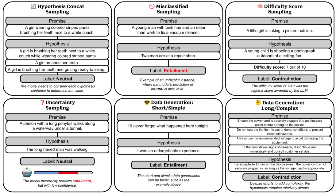
Figure 1: Examples of a training instance in $\mathcal{D}_{up}$ from our different methods.

3.5 Few-Shot LLM Data Generation

We generate additional, synthetic data using $\mathcal{M}$, our LLM before the fine-tuning, without relying on any external models. This data is produced in a zero-shot setting across a range of domains (see Appendix P), with each instance containing a single-sentence premise and hypothesis (Short & Simple Generation). We also use $\mathcal{M}$ to label unlabelled data generated for the MNLI Williams et al. (2018) training domains provided by Stacey and Rei (2024) (MNLI Domains Generation), which was generated by an older text-curie-001 GPT-3 model. To increase data complexity, we prompt the LLM to generate a four-sentence premise (Long & Simple Generation). To further raise the difficulty, we also prompt it to specify how the hypothesis relates to multiple parts of the premise, resulting in more contextually dependent examples (Long & Complex Generation - see Appendix M for details).

Finally, we investigate whether label quality can be improved, given that LLMs are known to be unreliable annotators. Models trained on LLM-generated labels can underperform compared to those trained on human annotated data Mohta et al. (2023), with previous work cautioning against fully relying on LLMs for annotation Ahmed et al. (2024); Brassard et al. (2022). While few-shot LLM annotation has shown promise for some tasks Calderon et al. (2025); Gilardi et al. (2023); Törnberg (2023), it remains unreliable for NLI Lu et al. (2023); Hosseini et al. (2024). Inspired by the if in doubt, discard approach from task-oriented dialogue Stacey et al. (2024a), we generate eight few-shot predictions from $\mathcal{M}$ per instance, and retain only those for which all predictions agree.

4 Experiments

		Challenge-OOD							Standard-OOD
	SNLI	r1	r2	r3	COPA	INLI-I	WANLI	Avg.	MNLI-m	MNLI-mm	FEVER	Scitail	INLI-NLI	Avg.
Encoder models (full training data):
RoBERTa-large	92.63	42.90	29.36	28.28	51.12	47.72	56.32	42.62	85.82	85.26	66.41	71.07	76.04	76.92
DeBERTa-base	92.64	40.34	34.08	31.82	50.92	36.88	57.91	41.99	84.68	85.25	63.68	75.82	72.17	76.32
DeBERTa-large	93.13	53.15	41.53	37.13	51.38	45.80	61.55	48.42	87.75	88.02	68.42	74.93	78.49	79.52
Debiasing methods w/ DeBERTa-large:
JTT	90.86	51.40	40.65	35.92	53.33	43.08	61.68	47.67$\downarrow$	85.47	85.70	67.06	74.09	77.52	77.97$\downarrow$
PoE	87.67	47.58	40.65	40.17	50.53	89.80	55.53	54.04$\uparrow$	79.43	79.21	62.43	81.60	69.68	74.47$\downarrow$
Reweight	91.78	52.35	41.80	40.33	50.30	67.55	59.56	51.98$\uparrow$	86.36	85.67	68.00	81.75	77.18	79.79$\uparrow$
LLMs (with 10,000 training instances):
Command R	91.14	63.58	55.78	52.88	56.60	66.84	61.21	59.48$\uparrow$	86.99	87.02	70.37	85.84	82.35	82.51$\uparrow$
Gemini-2.0-Flash	92.61	72.68	64.10	61.45	75.76	58.82	62.61	65.90$\uparrow$	88.30	88.54	71.56	73.42	85.09	81.38$\uparrow$
GPT-4o-mini	92.47	65.98	58.10	55.38	56.20	61.42	60.62	59.62$\uparrow$	86.93	87.24	71.21	72.55	80.21	79.63$\uparrow$

Table 1: The performance of RoBERTa Liu et al. (2019) and DeBERTa He et al. (2021, 2023a) models fine-tuned on the full SNLI training set are compared to Command R, Gemini-2.0-Flash and GPT-4o-mini models fine-tuned with just 10,000 instances. Accuracy is tested across a range our challenging NLI test sets (Challenge-OOD) and our other NLI test sets (Standard-OOD). We additionally measure performance of JTT, PoE and Example Reweighting for a DeBERTa-base model. The best results are in bold. $\uparrow$ and $\downarrow$ show better or worse average performance compared to the DeBERTa-large baseline.

We evaluate $\mathcal{M}$, $\mathcal{M}_{base}$ and each of our proposed methods on a diverse set of out-of-distribution NLI datasets, including WANLI Liu et al. (2022), ANLI Nie et al. (2020a), Scitail Khot et al. (2018), MNLI Williams et al. (2018), and INLI Havaldar et al. (2025). We also include FEVER-NLI Thorne et al. (2018); Nie et al. (2019), a fact verification dataset reformulated as NLI, and COPA-NLI, a new dataset we introduce by converting the Balanced-COPA commonsense QA dataset Kavumba et al. (2019); Gordon et al. (2012) into a challenging NLI test set (Appendix O). For INLI, we report separate results for the challenging implied entailment subset (INLI-I), and the remaining subset (INLI-NLI). We categorise each NLI dataset as either Challenge-OOD or Standard-OOD, defining Challenge-OOD as any dataset where our GPT-4o-mini baseline achieves below 70% accuracy. As a baseline, we also include Random Sampling, where we choose $\mathcal{D}_{up}^{c}$ as $\mathcal{K}$ randomly selected examples from $\mathcal{D}_{potential}^{c}$. We use SNLI Bowman et al. (2015) as our training data, with additional experiments using MNLI training data in Appendix D.

We test the robustness of three models available for fine-tuning as closed-source models: GPT-4o-mini (gpt-4o-mini-2024-07-18), Command R (base_type_chat), and Gemini-2.0-flash (gemini-2.0-flash-001). Unless stated otherwise, our experiments use GPT-4o-mini as a baseline. Despite the large cost involved, to mitigate the high variance in OOD predictions McCoy et al. (2020), each reported result is an average from fine-tuning five models using different random seeds.

Each of our proposed methods is designed without access to the out-of-distribution (OOD) data and uses no OOD-based hyper-parameter tuning. While tuning hyper-parameters on OOD data has been found to lead to strong robustness gains, we argue that this is a less realistic robustness setting. In our experiments, we set $\mathcal{K}$ to 5% of the training sample size, and fix $m$ at 10,000 training instances. We set $\mathcal{H}$ to be 3 for our Hypothesis Concat Sampling. When training the encoder models, we train the models with the full SNLI training data, in line with common practice. More detail about hyper-parameter choices can be found in Appendix N.

Finally, while some of the methods for identifying examples in $\mathcal{D}_{up}$ can also be used to identify examples for $\mathcal{D}_{down}$, this is not possible for all methods. Therefore, for comparability across methods, we choose $\mathcal{D}_{down}$ by random sampling from $\mathcal{D}_{init}$, avoiding making further changes to the training distribution. In Appendix H, we explore the effect of using alternative strategies for $\mathcal{D}_{\text{down}}$.

5 Results

		Challenge-OOD							Standard-OOD
	SNLI	r1	r2	r3	COPA	INLI-I	WANLI	Avg.	MNLI-m	MNLI-mm	FEVER	Scitail	INLI-NLI	Avg.
Baselines:
Baseline (10k)	92.47	65.98	58.10	55.38	56.20	61.42	60.62	59.62	86.93	87.24	71.21	72.55	80.21	79.63
Random Sampling	92.55	65.80	58.66	55.37	56.48	60.60	60.15	59.51$\downarrow$	86.94	87.00	71.17	69.56	81.15	79.16 $\downarrow$
Sampling:
Misclassified Sampling	92.32	65.48	57.98	52.73	62.94	56.88	60.32	59.39$\downarrow$	86.87	87.06	71.85	67.52	79.80	78.62 $\downarrow$
Hypothesis Concat Sampling	92.56	65.72	58.14	55.88	62.84	62.04	60.00	60.77$\uparrow$	86.55	86.69	70.81	69.88	80.71	78.93 $\downarrow$
Difficulty Score Sampling	92.66	67.48	59.10	56.42	58.84	59.54	61.40	60.46$\uparrow$	87.64	87.66	71.61	71.88	80.81	79.92 $\uparrow$
Uncertainty Sampling	92.80	67.42	58.60	55.12	63.68	60.60	60.99	61.07$\uparrow$	88.14	88.24	71.57	71.47	82.01	80.28 $\uparrow$
Generated Data:
MNLI Domains Generation	92.59	67.72	57.96	54.00	54.80	56.04	62.89	58.90$\downarrow$	87.79	88.34	72.97	80.98	85.90	83.20 $\uparrow$
Short & Simple Generation	92.47	68.88	58.14	53.43	56.28	52.02	64.11	58.81$\downarrow$	87.88	88.66	73.48	81.67	84.76	83.29 $\uparrow$
Long & Simple Generation	92.53	69.62	60.40	52.58	55.22	50.00	62.75	58.43$\downarrow$	88.08	88.88	73.05	78.97	83.33	82.46 $\uparrow$
Long & Complex Generation	92.64	67.24	59.04	56.03	55.68	61.14	60.35	59.91$\uparrow$	87.56	88.03	72.06	76.20	85.73	81.92 $\uparrow$

Table 2: Accuracy of GPT-4o-mini, fine-tuned with 10,000 training instances, compared to our sampling and synthetic methods for improving the robustness of this closed-source model. $\uparrow$ and $\downarrow$ show better or worse average performance compared to the baseline. The best results are in bold. See Appendix L for standard deviations.

5.1 Comparing LLMs to Encoder Models

Closed-source LLMs are considerably more robust than smaller encoder-based models, despite achieving similar in-distribution performance (Table 1). This gap is particularly noticeable for Challenge-OOD datasets, where LLMs outperform encoder models by more than 10 percentage points. Notably, this robustness is achieved using only 10,000 training instances – less than 2% of the 550k examples used to train each encoder. While encoder models perform competitively on WANLI, they perform poorly on each of the ANLI datasets and the INLI-implied examples (Table 1). On the Standard-OOD datasets, we also observe a degradation in performance, although this is not as pronounced.

Applying existing robustness methods can lead to some improvements on the Challenge-OOD datasets. Among them, Product of Experts has the largest improvement (+5.62% - see Table 1), however performance remains substantially below each of the LLMs tested. Just Train Twice reduces performance on Challenge-OOD (-0.75%) and Standard-OOD (-1.55%), which we analyse further in Appendix F.

Our findings suggest that smaller encoder models are no longer appropriate baselines for measuring model robustness, despite the continued use of these models Cheng and Amiri (2024); Honda et al. (2024); Koulakos et al. (2024); Stacey and Rei (2024); Zang and Liu (2024).

5.2 Few-shot Performance

As expected, we find that few-shot predictions from $\mathcal{M}$ are substantially worse on SNLI-test (-7.45%), but are also more robust, with improvements of 5.13% and 3.40% respectively on Challenge-OOD and Standard-OOD compared to $\mathcal{M}_{base}$ (see Appendix C). This contrasts with the findings from Mosbach et al. (2023), who compare models either using in-context learning or fine-tuning, with just 16 training examples. As we increase the size of the fine-tuning data, we find that in-distribution performance increases, but with no improvement in model robustness (see Appendix C).

5.3 Sampling Results

Selecting more complex examples for training leads to better performance on challenging out-of-distribution test sets (Table 2). These examples can also yield small improvements on less challenging test sets, although not consistently. Uncertainty Sampling is the most promising method, improving Challenge-OOD performance by an average of 1.45%, and Standard-OOD by 0.65% (Table 2). We also experiment with this method when training on MNLI, finding similar improvements (Appendix D). These improvements align with the intuition that instances with high prediction entropy represent ambiguous or under-represented cases in the training data. Including these examples helps the model generalise beyond overly confident or shortcut-driven examples.

Our next best method, Difficulty Score Sampling, improved performance on Challenge-OOD by 0.85%, but with smaller improvements on Standard-OOD. On the other hand, Hypothesis Concat Sampling improves performance on Challenge-OOD (+1.15%), although with a drop in performance on Standard-OOD (-0.69%).

Not all methods improve performance. Misclassified Sampling, inspired by Just Train Twice Liu et al. (2021), proves ineffective. A qualitative analysis of the examples chosen for $\mathcal{D}_{up}$ reveals a large number of annotation errors for this method (see Section 5.5), suggesting why performance is mostly worse with this method.

To better understand the magnitude of our improvements, we compare these improvements to prior work training on SNLI and evaluating on MNLI, a popular robustness setting (Table 3). Despite using a much stronger baseline, our improvements on MNLI are comparable in magnitude. We additionally analyse the hard, ambiguous and easy splits for MNLI-matched provided by Cosma et al. (2024), with each sampling method proving most effective on either the hard or the ambiguous test splits (Appendix E).

We explore variants of the best-performing methods. For Difficulty Score Sampling, we test alternative scoring functions, and for Uncertainty Sampling, we restrict upsampling to correctly predicted but uncertain examples. Neither adaptation yields further improvements (Appendix I). We also apply Uncertainty Sampling to maths datasets and observe a small performance gain, with average OOD accuracy increasing from 19.11 to 19.86 across seven different datasets (Appendix K).

		MNLI-m		MNLI-mm
Method	Baseline	Acc	Imp	Acc	Imp
Baselines (with OOD hyper-parameter tuning):
Hyp-only adversary1	LSTM	47.24	+1.38	49.24	+1.67
Ensemble-adversaries2	LSTM	54.18	+0.80	52.81	(0.10)
Product of Experts3	BERT	73.61	(0.79)	73.49	(0.49)
Debiased Focal Loss3	BERT	73.58	(0.82)	74.00	+0.02
Baselines (no OOD hyper-parameter tuning):
ATA, EBD-Reg4	BERT	72.51	+0.38	73.25	+0.85
Rationale supervision5	BERT	73.19	+0.91	73.36	+0.84
NILE6	RoBERTa	77.07	(2.22)	77.22	(2.07)
LIREx7	RoBERTa	79.85	(0.27)	79.79	+0.06
KD${}_{\text{ens}}$+aug8	DeBERTa	85.77	+1.21	86.18	+1.40
Our best methods:
Uncertainty Sampling	GPT-4o-mini	88.14	+1.21	88.24	+1.00
Short & Simple Generation	GPT-4o-mini	87.88	+0.95	88.66	+1.42
Long & Complex Generation	GPT-4o-mini	87.56	+0.63	88.03	+0.79

Table 3: Our most successful methods compared to improvements from prior work. ¹Belinkov et al. (2019a), ²Stacey et al. (2020), ³Mahabadi et al. (2020), ⁴Zang and Liu (2024), ⁵Stacey et al. (2022a), ⁶Kumar and Talukdar (2020), ⁷Zhao and Vydiswaran (2021), ⁸Stacey and Rei (2024).

5.4 Data Generation Results

		Challenge-OOD							Standard-OOD
	SNLI	r1	r2	r3	COPA	INLI-I	WANLI	Avg.	MNLI-m	MNLI-mm	FEVER	Scitail	INLI-NLI	Avg.
GPT-4o-mini:
Baseline (10k)	92.47	65.98	58.10	55.38	56.20	61.42	60.62	59.62	86.93	87.24	71.21	72.55	80.21	79.63
Short & Simple Generation	92.47	68.88	58.14	53.43	56.28	52.02	64.11	58.81$\downarrow$	87.88	88.66	73.48	81.67	84.76	83.29 $\uparrow$
Long & Complex Generation	92.64	67.24	59.04	56.03	55.68	61.14	60.35	59.91$\uparrow$	87.56	88.03	72.06	76.20	85.73	81.92 $\uparrow$
Command R:
Baseline (10k)	91.14	63.58	55.78	52.88	56.60	66.84	61.21	59.48$\uparrow$	86.99	87.02	70.37	85.84	82.35	82.51
Short & Simple Generation	91.04	61.48	52.50	50.23	54.30	58.10	62.11	56.45$\downarrow$	87.79	87.68	71.09	88.47	83.19	83.64$\uparrow$
Long & Complex Generation	91.46	62.62	54.34	52.12	55.00	64.60	60.02	58.12$\downarrow$	86.81	87.10	71.27	85.27	85.43	83.18$\uparrow$
Gemini-2.0-Flash:
Baseline (10k)	92.61	72.68	64.10	61.45	75.76	58.82	62.61	65.90	88.30	88.54	71.56	73.42	85.09	81.38
Short & Simple Generation	92.71	75.90	65.38	62.47	83.46	67.08	64.73	69.84$\uparrow$	88.82	88.53	72.94	77.94	67.08	82.94$\uparrow$
Long & Complex Generation	92.54	76.28	67.22	64.28	68.28	66.36	62.78	67.53$\uparrow$	88.61	89.01	73.01	75.30	87.67	82.72$\uparrow$

Table 4: Testing our data generation methods for GPT-4o-mini, Command R and Gemini-2.0-Flash. As Command R and Gemini do not provide probability scores, we do not also test our Uncertainty Sampling method.

Adding LLM-generated synthetic data during training substantially improves performance on Standard-OOD, with gains ranging from 2.29% to 3.66% across methods. Table 2 shows that every Standard-OOD test set benefits from the inclusion of synthetic data.

Due to the relatively simple entailment relationships provided in our synthetic data, we mostly see a reduction in performance on Challenge-OOD (see Table 2). An exception is the Long & Complex Generation, which maintains the baseline performance on Challenge-OOD. Interestingly, simply increasing premise length does not lead to any improvements, with the Short & Simple Generation outperforming the Long & Simple Generation for both Challenge-OOD and Standard-OOD. This suggests that the benefit of synthetic examples lies less in their surface complexity (e.g., length), and more in the diversity or novelty of entailment relationships they introduce. Simply adding verbose inputs may not increase semantic difficulty.

We additionally test our data generation methods with Command R and Gemini-2.0-Flash (Table 4), finding that both the Short & Simple and the Long & Complex Generation methods improve performance on Standard-OOD. Across models, the Short & Simple Generation consistently outperforms the Long & Complex Generation on Standard-OOD, while the Long & Complex Generation performs better on Challenge-OOD.

We test whether the if in doubt, discard validation method is necessary for strong performance with LLM-generated data. The validation improves Challenge-OOD performance for the Long & Complex Generation method (+1.30%; see Appendix G), but has no impact on Standard-OOD or when applied to the MNLI Domains Generation method. These results suggest that the validation method is most beneficial when applied to more challenging synthetic examples. Finally, when training on MNLI instead of SNLI, we find that improvements are limited to Challenge-OOD (see Long & Complex Generation, Appendix D), suggesting that the additional synthetic data is most helpful for single domain datasets.

5.5 Analysis of $\mathcal{D}_{up}$

We analyse the examples selected for $\mathcal{D}_{up}$ by manually inspecting 50 examples per method and assigning a difficulty score between 1-10. We also review the label annotations for each method.

Misclassified Sampling has both the highest average difficulty score (5.92), and the most annotation errors (54%). The next highest difficulty score is from Uncertainty Sampling (5.26), with an annotation error rate of 24%. There is a large overlap between the two methods, with 33.1% of $\mathcal{D}_{up}$ shared between the two methods. Uncertainty Sampling appears to retain many of the valuable examples from Misclassified Sampling while avoiding its high rate of label errors.

Difficulty Score Sampling yields a lower average difficulty score (4.44) but also fewer annotation errors (16%). This difficulty score remains higher than that of the original SNLI training data (3.84), which contains only 4% annotation errors.

For the data generation methods, the Long & Complex Generation produces more difficult examples than the original training data (average difficulty score of 4.52 vs. 3.84), while the Short & Simple Generation yields less difficult examples (3.40). Both methods have fewer annotation errors than the sampling approaches, with rates of 12% and 4% respectively.

5.6 Summary of Findings

Across our experiments, we find that closed-source LLMs substantially outperform encoder-based models in robustness, despite being fine-tuned on less than 2% of the data. Among sampling strategies, Uncertainty Sampling consistently yields the strongest improvements on Challenge-OOD datasets, while Short & Simple Generation proves most effective for improving Standard-OOD performance. The effectiveness of each method depends not only on example difficulty but also on label quality: Misclassified Sampling selects difficult but noisy examples, whereas Uncertainty Sampling achieves a better trade-off between informativeness and correctness. For generation-based methods, more complex examples such as those in Long & Complex Generation help preserve or improve performance on harder test sets. Our findings highlight the importance of carefully balancing difficulty and reliability when constructing training data for more robust fine-tuned models.

6 Discussion

6.1 Task Subjectivity

Labelling entailment relationships can be subjective, either because of different, valid interpretations of the same instance Liu et al. (2022), or due to the ambiguous definitions of each class Pavlick and Kwiatkowski (2019). Instead, entailment relationships could be better understood as a likelihood rather than using discrete entailment labels Zhang et al. (2017); Nie et al. (2020b). We find that this task ambiguity is a particular issue for OOD evaluation, with subtle differences in how the task is interpreted across different datasets. For example, there can be different assumptions about how likely an entailment hypothesis should be, and whether relevant background knowledge needs to be explicitly stated in the premise. For example, in SNLI no explicit evidence is required in the premise to support the hypothesis ‘The boy has one head’, but in Scitail the hypothesis ‘One example of matter is water’ is not always entailed.

6.2 OOD Dataset Selection

The most popular datasets for measuring NLI robustness have been adversarial test sets associated with specific biases, such as HANS McCoy et al. (2019), SNLI-hard Gururangan et al. (2018), or the NLI stress tests Naik et al. (2018). While some previous work evaluates on a wider range of out-of-distribution test sets, this often relies on hyper-parameter tuning on the out-of-distribution data Belinkov et al. (2019a); Stacey et al. (2020); Mahabadi et al. (2020, 2021). By using modern LLMs as our baseline models, we have been able to measure model robustness on a wider range of challenging OOD NLI datasets, providing a more comprehensive measure of model robustness.

6.3 Human Annotated Data vs Synthetic Data

Replacing LLM generated data with human annotated data has previously been shown to improve performance Mohta et al. (2023), even if only replacing a small sample of examples Ashok and May (2024). However, the success of LLM-generated data depends on both the task, and the level of expertise of the annotator Calderon et al. (2025), which is often crowd-source workers for NLI. We argue that using synthetically generated training data is particularly helpful for improving robustness, as it can offer a different distribution from the human annotated training data. We suggest that these benefits can often outweigh issues with label quality.

7 Conclusion

We investigate methods for improving the robustness of closed-source fine-tuned LLMs, aiming to maintain the strong in-distribution performance achieved after fine-tuning, while also mitigating the corresponding loss in model robustness. We find that for the most complex OOD data, the best strategy is to train with more challenging training examples. However, for less challenging OOD data, replacing some of the training examples with LLM-generated data is the best strategy and can lead to substantial improvements.

Finally, our results show that LLMs are considerably more robust than existing encoder model baselines, especially on challenging OOD test sets, and we advocate for using these models as baselines for future work improving NLI robustness.

Appendix A Additional Related Work

A.1 Model Debiasing

Model centric debiasing methods for NLI mostly involve either weighting the loss of training examples based on a bias models predictions Mahabadi et al. (2020); Clark et al. (2019); Ghaddar et al. (2021); Du et al. (2023b); Rajic et al. (2022); Xiong et al. (2021), adding the bias model soft predictions, log probabilities, or attention scores during training to encourage the model to instead focus on unbiased features Mahabadi et al. (2020); Clark et al. (2019); He et al. (2019); Sanh et al. (2021); Wang et al. (2023a); Xiong et al. (2021), adjusting a model’s soft probabilities at inference time based on the predictions of a biased model Udomcharoenchaikit et al. (2022); Tian et al. (2022), or encouraging a model to be less confident when a bias model or perturbed input can result in correct predictions Utama et al. (2020a); Cheng and Amiri (2024); Du et al. (2021). Each of these methods accommodate a variety of ways of choosing the bias model, which include identifying specific dataset biases He et al. (2019); Clark et al. (2019); Du et al. (2023b), including the hypothesis-only NLI bias Mahabadi et al. (2020); He et al. (2019), using models that are not large enough Sanh et al. (2021); Clark et al. (2020) or do not contain enough training data Utama et al. (2020b), or finally, using features from earlier layers in the model Wang et al. (2025); Ghaddar et al. (2021).

For LSTM models Hochreiter and Schmidhuber (1997), adversarial training has also been effective at removing dataset biases, either removing these biases from a model representations Belinkov et al. (2019a, b); Stacey et al. (2020) or embeddings Zhou and Bansal (2020). Despite the success of adversarial training with LSTM models, we are not aware of any work showing that these methods can also be successfully applied to transformer-based NLI models.

A.2 Data Augmentation

An increasingly common approach for improving model robustness involves exploiting recent advances in LLMs to generate synthetic datasets, creating large volumes of additional training data. This additional training data has proved helpful, both for improving robustness Hosseini et al. (2024); Chen et al. (2023); Wang et al. (2023b); Liu et al. (2022); Wu et al. (2022) and improving in-distribution performance Banerjee et al. (2024b). Instead of using LLMs to generate additional training instances, new examples can also be created by perturbing existing training examples Minervini and Riedel (2018); Zhou and Bansal (2020); Liu et al. (2020); Min et al. (2020). This can involve paraphrasing Zhou and Bansal (2020), swapping the subject and object in the input sentences Min et al. (2020), adding additional text at the end of the inputs Zhou and Bansal (2020), swapping the hypothesis and premise Liu et al. (2020), or using first-order logic rules Minervini and Riedel (2018). New examples can also be created using human annotation Kaushik et al. (2020); Yanaka et al. (2019); He et al. (2023b).

Whether human-annotated or LLM generated, augmented data used to improve robustness is either: 1) created by making small changes to either the hypothesis or premise Chen et al. (2023); Yanaka et al. (2019); Min et al. (2020); Wen et al. (2022), 2) created to be similar to challenging or unbiased examples in the training domain Liu et al. (2022); Wu et al. (2022); He et al. (2023b); Wang et al. (2023b), or 3) created as entirely new instances in different domains Hosseini et al. (2024); Stacey and Rei (2024).

A.3 Data Filtering

Rather than augment a dataset with additional examples, a dataset can be filtered to remove biased examples Wu et al. (2022); Bras et al. (2020a), helping to improve robustness. In its simplest form, dataset filtering can involve a filtering process to remove examples that have been identified as having a sufficient level of bias Ravichander et al. (2023). Wu et al. (2022) introduce an algorithm for iteratively removing biased instances, considering whether hand-crafted features correlate to a specific class using z-statistics Gardner et al. (2021). Alternatively, Bras et al. (2020b) iteratively partition a dataset into a train and test partition, training on the training examples, before evaluating on the test examples. This process is repeated, each time choosing different train and test splits, with examples filtered out which are most commonly predicted as the correct label when they are in the test split. This process is repeated for a set number of steps, resulting in a reduced, less biased dataset.

A.4 Improving Robustness with Explanations

Recent work has also investigate whether NLI robustness can be improved with the use of explanations, using human annotated explanations during training Stacey et al. (2022a); Ross et al. (2022); Koulakos et al. (2024); Zang and Liu (2024) with the e-SNLI human annotated explanations Camburu et al. (2018). Models can learn from the human explanations by supervising the CLS token in the final layer of the model Stacey et al. (2022a), or by training models to generate explanations alongside making class label predictions Ross et al. (2022); Koulakos et al. (2024); Ludan et al. (2023). However, not all past work using explanations during training has led to improvements in robustness (Kumar and Talukdar, 2020; Zhao and Vydiswaran, 2021; Camburu et al., 2018). Recent work has also tested whether including chain of thought explanations with in-context examples improves robustness Mueller et al. (2024); He et al. (2024b), with mixed results.

A.5 Learning from Minority Examples

Minority examples can be defined as instances that counter common spurious patterns in a dataset Tu et al. (2020). Modifying the training process can help models to learn more from these minority examples, improving out-of-distribution performance for NLI Korakakis and Vlachos (2023); Liu et al. (2021); Yaghoobzadeh et al. (2021). Liu et al. (2021) test a fine-tuned model on its own training data, identifying minority examples as the instances misclassified in the training set. Then these examples were upsampled during a second round of training. Similarly, Yaghoobzadeh et al. (2021) identify training examples that were misclassified, but also including examples that were predicted as the wrong class at some point during training. A second phase of training then trained only on these minority examples. Rather than identifying minority examples as those that a single model has misclassified, ensembles can also be used to better identify these examples, with minority examples defined as any training instance that any model in an ensemble has incorrectly predicted Stacey and Rei (2024).

A.6 Improving Robustness with Knowledge Distillation

NLI robustness has also been studied in the context of knowledge distillation, where the distillation process is modified to produce more robust student models. This can involve smoothing the teacher soft predictions Du et al. (2023a); Jafari et al. (2021), or applying methods inspired by Just Train Twice Liu et al. (2021) to learn more from challenging examples Du et al. (2023a); Stacey and Rei (2024). Using additional unlabelled examples can also improve the robustness of NLI student models, generating additional examples by masking individual words and adversarially generating words to replace these masks Rashid et al. (2021); Li et al. (2021); Haidar et al. (2022), or using LLMs to generate unlabelled data that can be used during distillation Stacey and Rei (2024).

A.7 Distributionally Robust Optimization

Sagawa et al. (2020) demonstrate how Distributionally Robust Optimization (DRO) can improve the robustness of NLI models, training models with the objective of minimising the worst-group loss. Sagawa et al. (2020) segment MNLI instances into groups based on the class (entailment, neutral or contradiction), and whether there is a negation term present, creating six groups from these different possible combinations. During training, the loss for instances in each group are adjusted, with this adjustment depending on the loss so far during training for the groups they belong to. Sagawa et al. (2020) find that DRO improves the robustness on instances belonging to the worst group during inference, although with lower overall performance. Rather than using known heuristics, subsequent work has identified automatic methods for identifying the training groups Bao and Barzilay (2022); Bao et al. (2021); Paranjape et al. (2023). The worst-group performance tested by Sagawa et al. (2020) can also be improved by simply adjusting the class imbalance between groups in the training data Idrissi et al. (2021).

A.8 Atomic Decomposition Methods

The task of NLI can be decomposed into different atoms, with predictions made separately for individual atoms. These predictions are then aggregated into instance-level model predictions, with some evidence this can lead to robustness improvements. The atom-level decomposition can involve segmenting hypotheses into spans, and making predictions for each hypothesis span independently, which can improve robustness when there is limited training data Stacey et al. (2022b). Alternatively, decomposing each premise into a list of atomic facts, and making predictions for each premise fact independently can result in out-of-distribution improvements Stacey et al. (2024b).

Rather than decompose each hypothesis or premise, Negru et al. (2025) train a model to edit (or morph) a premise step by step until it matches the hypothesis, using a fine-tuned NLI model to track how entailment changes over these intermediate steps. During inference, model predictions are aggregated based on the entailment predictions at each step, decomposing the task into a series of smaller inference steps. This decomposition process was found to improve the model’s generalisation abilities. Symbolic methods can also improve robustness, with Kalouli et al. (2020) using a symbolic approach (combined with a standard neural model) to make predictions based on the differences between the premise and hypothesis. This also resulted in NLI out-of-distribution improvements.

A.9 Further NLI Robustness Strategies

Further strategies to improve NLI robustness include: supervising gradients of instances based on the difference between each instance and a corresponding counterfactual Teney et al. (2020), using Variational Information Bottleneck’s to improve the robustness of models in a low resource setting Mahabadi et al. (2021), and introducing a mixture of experts model that trains different classifiers on top of a BERT encoder, weighting the soft probabilities of each expert Honda et al. (2024). Finally, Lee et al. (2025) find that using prompt tuning can improve robustness compared to other fine-tuning strategies, tuning the prompt tokens that have the least importance for dev set predictions.

Appendix B Notation for Dataset Subsets

Symbol	Description
$\mathcal{D}$	Full NLI dataset (all available annotated examples).
$\mathcal{D}_{\text{init}}$	Initial training subset used to fine-tune the base model ($|\mathcal{D}_{\text{init}}|=m$).
$\mathcal{D}_{\text{potential}}$	Candidate examples from $\mathcal{D}\setminus\mathcal{D}_{\text{init}}$ considered for upsampling.
$\mathcal{D}_{\text{up}}$	New, challenging examples selected to improve robustness.
$\mathcal{D}_{\text{down}}$	Subset of $\mathcal{D}_{\text{init}}$ removed to make room for $\mathcal{D}_{\text{up}}$, preserving fixed budget.

Table 5: Notation summary for dataset subsets used in our training strategies.

To aid readability, we provide a summary of the dataset subsets in Table 5 used throughout our methods section. This includes the roles of each subset in training and evaluation.

Appendix C Baseline Analysis

We experiment with training our baseline model $\mathcal{M}_{base}$ with 5k, 10k and 20k training instances, to understand whether training with more data improves in-distribution or out-of-distribution performance (Table 6). Overall, we find that more fine-tuning data improves in-distribution performance, but without improvements in model robustness. Our few-shot baseline using $\mathcal{M}$ is substantially worse on SNLI-test, but also substantially more robust on Standard-OOD and Challenge-OOD.

		Challenge-OOD							Standard-OOD
	SNLI	r1	r2	r3	COPA	INLI-I	WANLI	Avg.	MNLI-m	MNLI-mm	FEVER	Scitail	INLI-NLI	Avg.
GPT-4o-mini baselines:
5k baseline	92.18	65.92	57.70	55.68	56.40	61.04	61.51	59.71	86.93	87.46	71.45	76.54	82.38	80.95
10k baseline	92.47	65.98	58.10	55.38	56.20	61.42	60.62	59.62	86.93	87.24	71.21	72.55	80.21	79.63
20k baseline	92.78	66.06	57.54	54.83	58.98	60.54	59.46	59.57	87.32	87.10	71.20	69.65	80.61	79.18
Few-shot baseline	85.02	77.00	63.90	58.33	63.60	60.80	64.88	64.75	84.62	85.09	73.53	84.62	87.30	83.03

Table 6: We compare our baseline with 10k training instances to a baseline with twice this amount, showing that more training examples has led to better robustness, but worse performance on SNLI-test. As expected, we also show that our baseline has substantially better performance than a few-shot baseline $\mathcal{M}$. Unlike all previous experiments, the few-shot baseline uses a single seed rather than an average of 5 seeds.

Appendix D Experiments Training on MNLI

		Challenge-OOD							Standard-OOD
	MNLI-m	r1	r2	r3	COPA	INLI-I	WANLI	Avg.	SNLI-dev	SNLI-test	FEVER	Scitail	INLI-NLI	Avg.
GPT-4o-mini - MNLI training data:
Baseline (10k)	90.73	68.72	56.56	52.58	50.08	47.10	65.54	56.76	91.81	91.38	73.18	85.58	86.05	85.60
Uncertainty Sampling	91.09	70.80	58.68	54.53	50.02	49.48	65.57	58.18$\uparrow$	91.43	91.10	73.45	85.52	86.53	85.61$\uparrow$
Short & Simple Generation	90.45	68.17	55.84	52.08	50.14	46.28	66.45	56.50$\downarrow$	91.38	91.08	73.42	85.79	86.08	85.55$\downarrow$
Long & Complex Generation	90.52	67.92	57.12	53.85	50.70	50.32	65.14	57.51$\uparrow$	91.71	91.34	73.59	85.97	86.81	85.88$\uparrow$

Table 7: We experiment with our best performing methods when training on MNLI, a dataset with five different training domains.

We additionally experiment with using MNLI as our training data instead of SNLI, while replacing the MNLI-matched and MNLI-mismatched validation sets in Standard-OOD with SNLI-dev and SNLI-test. Similar to our results with the SNLI training data, we find improvements on Challenge-OOD when using Uncertainty Sampling (+1.42, see Table 7). These improvements are of a similar magnitude to the improvements observed when training on SNLI (+1.45, see Table 2). Using the Uncertainty Sampling method with MNLI training data also maintains the baseline performance on Standard-OOD (+0.01%, see Table 7).

We find that the Long & Complex Generation method also improves performance on Challenge-OOD (+0.75, see Table 7). This is a larger improvement compared to our results training on SNLI (+0.29, see Table 7). However, unlike our experiments training on SNLI, we do not see the same performance improvements on Standard-OOD from our data generation methods. As the MNLI training data already contains data from five different domains, we suggest that including additional, diverse LLM-generated training data is less beneficial in this case.

Appendix E Additional SNLI and MNLI analysis

We use the hard, ambiguous and easy splits provided by Cosma et al. (2024) to understand why our methods have a performance advantage when evaluated on MNLI, and whether this is driven by improvements on more challenging examples. Table 8 shows how the out-of-distribution improvements on MNLI from our sampling methods are largest on either the hard or the ambiguous test splits. For Misclassified Sampling and Difficulty Score Sampling, the largest performance improvement is on the Hard test set, whereas for Hypothesis Concat Sampling and Uncertainty Sampling the largest increase is on the Ambiguous test set. For SNLI, the differences between the baseline and our method are smaller, with our methods providing no clear advantage over the baseline model.

For the data generation methods, we consistently see improvements on the Easy test split. However, surprisingly, there are also improvements on the Hard test splits when using the LLM-generated synthetic data.

	SNLI			MNLI-m
Method	Hard	Amb.	Easy	Hard	Amb.	Easy
Baselines:
GPT-4o-mini	67.98	89.68	97.47	59.27	80.90	91.89
Our methods:
Misclassified Sampling	68.20	89.44	97.27	60.49	80.65	91.69
Difficulty Score Sampling	67.85	89.98	97.68	61.30	81.25	92.49
Hypothesis Concat Sampling	67.80	90.18	97.50	58.30	81.56	91.39
Uncertainty Sampling	68.20	90.04	97.81	61.01	82.31	92.99
Short and Simple Generation	68.15	89.70	97.43	64.42	77.55	93.08
Long & Simple Generation	67.97	89.69	97.56	63.65	79.54	93.08
Long & Complex Generation	68.05	89.99	97.62	59.31	81.13	92.68

Table 8: Performance of our methods on Hard, Ambiguous and Easy test splits of SNLI and MNLI-matched.

Appendix F Just Train Twice Further Analysis

		Challenge-OOD							Standard-OOD
	SNLI	r1	r2	r3	COPA	INLI-I	WANLI	Avg.	MNLI-m	MNLI-mm	FEVER	Scitail	INLI-NLI	Avg.
RoBERTa-large
Baseline	92.63	42.90	29.36	28.28	51.12	47.72	56.32	42.62	85.82	85.26	66.41	71.07	76.04	76.92
With Just Train Twice	89.08	39.64	30.94	29.03	51.36	41.31	56.15	40.81	79.24	79.39	63.92	68.97	72.07	72.72
DeBERTA-base
Baseline	92.64	40.34	34.08	31.82	50.92	36.88	57.91	41.99	84.68	85.25	63.38	75.82	72.17	76.32
With Just Train Twice	89.49	40.12	34.86	31.53	51.96	36.60	56.92	42.00	80.50	81.78	62.97	75.71	69.94	74.18
DeBERTA-large:
Baseline	93.13	53.15	41.53	37.13	51.38	45.80	61.55	48.42	87.75	88.02	68.42	74.93	78.49	79.52
With Just Train Twice	90.86	51.40	40.65	35.92	53.33	43.08	61.68	47.68$\uparrow$	85.47	85.70	67.06	74.09	77.52	77.97$\downarrow$

Table 9: The performance of RoBERTa Liu et al. (2019) and DeBERTa He et al. (2021, 2023a) baseline models, and the same models after applying Just Train Twice.

To better understand the impact of Just Train Twice (JTT) on different encoder models, we try implementing this method with DeBERTa-base, DeBERTa-large and RoBERTa-large. In each case, we find no improvements compared to the baseline, with a large drop in performance on the Standard-OOD test sets (see Table 9).

We further investigate whether JTT can help on adversarial tests sets designed around specific biases. We find that after training on MNLI, OOD performance increases on HANS from 75.88% to 76.93% when applying JTT. Our results suggest that JTT can be effective for specific challenge test sets, but this method often does not improve robustness more generally across a wider range of OOD test sets.

Appendix G If in Doubt, Discard Validation

We investigate the effect of using if in doubt, discard validation to improve the quality of our labelled data. While there is an improvement of 1.30% for the Long & Complex Generation on Challenge-OOD (Table 10), there is no corresponding improvement on Standard-OOD. We also find little difference in performance on the MNLI Domains Generation, for either Challenge-OOD or Standard-OOD. We conclude that the if in doubt, discard validation is helpful for the most complex LLM-generated data, but is otherwise not required.

		Challenge-OOD							Standard-OOD
	SNLI	r1	r2	r3	COPA	INLI-I	WANLI	Avg.	MNLI-m	MNLI-mm	FEVER	Scitail	INLI-NLI	Avg.
GPT-4o-mini - MNLI Domains Generation:
Without validation	92.48	68.56	58.08	54.18	52.96	54.92	63.02	58.62	87.71	88.20	73.39	81.23	86.21	83.35
With Validation	92.59	67.72	57.96	54.00	54.80	56.04	62.89	58.90	87.79	88.34	72.97	80.98	85.90	83.20
GPT-4o-mini - Long & Complex Generation:
Without validation	92.48	68.52	59.74	52.22	57.58	50.34	63.26	58.61	88.02	88.74	73.03	79.67	83.34	82.56
With Validation	92.64	67.24	59.04	56.03	55.68	61.14	60.35	59.91	87.56	88.03	72.06	76.20	85.73	81.92

Table 10: We compare results for our data generation methods, showing performance with and without the if in doubt, discard validation.

Appendix H Selecting both $\mathcal{D}_{down}$ and $\mathcal{D}_{up}$

		Challenge-OOD							Standard-OOD
	SNLI	r1	r2	r3	COPA	INLI-I	WANLI	Avg.	MNLI-m	MNLI-mm	FEVER	Scitail	INLI-NLI	Avg.
GPT-4o-mini - Uncertainty Sampling:
Up selection	92.80	67.42	58.60	55.12	63.68	60.60	60.99	61.07	88.14	88.24	71.57	71.47	82.01	80.28
Up and down	92.83	67.16	59.54	54.97	60.14	60.74	61.51	60.68	87.93	88.11	71.46	71.93	82.33	80.35$\uparrow$
GPT-4o-mini - Difficulty Score Sampling:
Up selection	92.66	67.48	59.10	56.42	61.40	60.46	61.51	60.68	87.64	87.66	71.64	71.88	80.81	79.92
Up and down	92.68	66.86	57.96	56.35	57.58	64.94	60.39	60.68	86.77	86.96	71.18	71.38	81.12	79.48

Table 11: We experiment with selecting new examples for $\mathcal{D}_{up}$ using our Uncertainty Sampling, while also choosing examples for $\mathcal{D}_{down}$ as the most confident predictions within $\mathcal{D}_{init}$. ‘Up selection’ refers to the Uncertainty Sampling method defined in the paper, where we choose examples based on their uncertainty, and randomly choose examples in $\mathcal{D}_{init}$ for $\mathcal{D}_{down}$. ‘Up and down’ also chooses $\mathcal{D}_{down}$ based on model confidence. We also perform a similar experiment with our Difficulty Score Sampling method, choosing $\mathcal{D}_{down}$ based on the lowest difficulty scores.

We experiment with using our sampling methods to choose both $\mathcal{D}_{down}$ and $\mathcal{D}_{up}$, using both the Uncertainty Sampling and Difficulty Score Sampling methods. For Uncertainty Sampling, we choose $\mathcal{D}_{up}$ as the examples with the highest entropy in $\mathcal{D}_{potential}$, while choosing $\mathcal{D}_{down}$ as the examples with the lowest entropy in $\mathcal{D}_{init}$. Similarly, for Difficulty Score Sampling, we choose $\mathcal{D}_{down}$ as the examples in $\mathcal{D}_{init}$ with the lowest difficulty score.

We find that using our methods to also select examples for $\mathcal{D}_{down}$ makes little difference to performance (Table 13). This suggests that additionally including a small number of complex examples has a much greater effect than removing a small number of easier examples from the model’s training data.

Appendix I Difficulty Score Sampling

		Challenge-OOD							Standard-OOD
	SNLI	r1	r2	r3	COPA	INLI-I	WANLI	Avg.	MNLI-m	MNLI-mm	FEVER	Scitail	INLI-NLI	Avg.
GPT-4o-mini - Difficulty Score Sampling:
C + D	92.55	67.42	58.34	54.98	57.58	59.54	61.08	59.82	87.93	87.79	71.59	70.62	80.61	79.71
D	92.66	67.48	59.10	56.42	61.40	60.46	61.51	60.68	87.64	87.66	71.64	71.88	80.81	79.92
C + D + P + F	92.41	67.92	57.94	55.50	59.64	56.32	61.07	59.73	87.94	87.82	71.35	72.39	80.93	80.09

Table 12: We experiment with different methods for combining the scores provided by the baseline model $\mathcal{M}$ before fine-tuning. These scores are identified by asking the model to make few-shot assessments about the examples in $\mathcal{D}_{potential}$. The available scores are: C (correctness), D (difficulty), P (plausibility), F (fluency). C + D is the configuration used in the main paper.

We investigate introducing a wider range of scores to measure the quality of NLI training examples, beyond the difficulty score used within our Difficulty Score Sampling. We try two different configurations, firstly including a score for label quality and summing this together with the difficulty score, and secondly, also adding scores for the plausibility and fluency of the instances (see Table 12).

While using the combination of all of the scores (difficulty, correctness, plausibility and fluency) performs slightly better on Standard-OOD, performance is worse on Challenge-OOD. We conclude that including the additional scores does not help to improve model robustness.

Appendix J Uncertainty Sampling

		Challenge-OOD							Standard-OOD
	SNLI	r1	r2	r3	COPA	INLI-I	WANLI	Avg.	MNLI-m	MNLI-mm	FEVER	Scitail	INLI-NLI	Avg.
GPT-4o-mini - Uncertainty Sampling:
Uncertainty Sampling	92.80	67.42	58.60	55.12	63.68	60.60	60.99	61.07	88.14	88.24	71.57	71.47	82.01	80.28
Uncertainty Sampling (correct only)	92.68	66.90	57.52	54.88	57.10	59.06	61.62	59.51	88.21	88.24	71.77	75.39	80.88	80.90

Table 13: We experiment with only choosing examples for $\mathcal{D}_{up}$ for Uncertainty Sampling if the predictions from the baseline model $\mathcal{M}_{base}$ are correct.

With the aim of reducing label noise with our Uncertainty Sampling method, we experiment with only choosing examples for $\mathcal{D}_{up}$ which are correctly predicted by $\mathcal{M}$ (see Table 13). This means we choose examples where the model is correct, but still uncertain. We find however that this restriction results in worse robustness on Challenge-OOD, presumably because the selected examples are now less complex. We do however find a small improvement in Standard-OOD performance.

Appendix K Maths Datasets

	ID		OOD
	Calc-Ape210k	AQuA-RAT	MinervaMath	MATH500	Omni-MATH500	AMC23	OlympiadBench	HMMT	Avg.
Few-shot	29.02	30.73	14.66	22.73	12.46	20.00	9.31	1.14	15.86
10k baseline	49.05	32.11	36.44	23.74	13.84	16.50	10.02	1.14	19.11
Uncertainty Sampling ($\mathcal{K}$ = 15%)	49.24	33.67	36.65	23.33	14.25	14.50	10.61	1.81	19.26
Uncertainty Sampling ($\mathcal{K}$ = 50%)	48.74	32.93	37.70	23.08	14.58	19.00	10.14	1.59	19.86

Table 14: We test our Uncertainty Sampling method on maths datasets after training on 10k instances from Calc-Ape, before testing performance on other out-of-distribution maths datasets. We experiment with selecting $\mathcal{K}$ = |$\mathcal{D}_{up}$| = 0.15 $\times$ |$\mathcal{D}_{init}$|, similar to our NLI experiments, and $\mathcal{K}$ = |$\mathcal{D}_{up}$| = 0.50 $\times$ |$\mathcal{D}_{init}$|.

As our Uncertainty Sampling method is directly applicable to a range of other NLP tasks, we experiment with applying this method to maths datasets. We train our model on 10,000 instances from Calc-Ape210k Kadlčík et al. (2023), before evaluating on AQuA-RAT Ling et al. (2017), MinervaMATHLewkowycz et al. (2022), MATH500 Lightman et al. (2024), Omni-MATH500 Gao et al. (2025), AMC23 Yang et al. (2024), OlympiadBench He et al. (2024a) and HMMT Roucher et al. (2025). Similar to our experiments with NLI, with aim to evaluate out-of-distribution performance on a wide range of datasets.

For AQuA-RAT, we predict numerical answers rather than choosing multiple choice labels (also without providing the model with the multiple choice answers in the prompt). We also remove questions requiring “All of the above” or “None of the above” as answers, reducing the test set from 254 to 218 samples. For MinervaMATH, MATH500, Omni-MATH500, OlympiadBench and HMMT we remove questions with answers that are not a number. This reduces the test sets to 191, 396, 321, 505 and 88 instances respectively. For HMMT, this involves merging HMMT Feb. 23, HMMT Feb 24 and HMMT Feb. 25. To be consistent with our NLI experiments, and to avoid larger fine-tuning costs, we do not train our model to generate chain-of-thought answers.

We experiment with $\mathcal{K}$ = |$\mathcal{D}_{up}$| = 0.15 $\times$ |$\mathcal{D}_{init}$|, similar to our NLI experiments. But unlike NLI, there is less variety in the complexity of the different training examples in Calc-Ape210k, so we also experiment with $\mathcal{K}$ = |$\mathcal{D}_{up}$| = 0.50 $\times$ |$\mathcal{D}_{init}$|. We find that when we set $\mathcal{K}$ = |$\mathcal{D}_{up}$| = 0.50, Uncertainty Sampling improves out-of-distribution performance by 0.75% percentage points (from 19.11% to 19.86%), an increase of 3.9%.

Appendix L Method Standard Deviations

		Challenge-OOD							Standard-OOD
	SNLI	r1	r2	r3	COPA	INLI-I	WANLI		MNLI-m	MNLI-mm	FEVER	Scitail	INLI-NLI
Baselines:
Baseline (10k)	0.001	0.008	0.011	0.009	0.023	0.043	0.007		0.005	0.007	0.007	0.034	0.012
Random sampling	0.001	0.007	0.014	0.017	0.047	0.053	0.017		0.009	0.011	0.010	0.025	0.007
Sampling:
Misclassified Sampling	0.002	0.012	0.008	0.022	0.077	0.067	0.014		0.007	0.009	0.007	0.017	0.010
Hypothesis Concat Sampling	0.001	0.017	0.011	0.011	0.075	0.041	0.009		0.007	0.006	0.008	0.024	0.009
Difficulty Score Sampling	0.002	0.011	0.015	0.023	0.031	0.054	0.014		0.006	0.007	0.006	0.027	0.011
Uncertainty Sampling	0.002	0.015	0.016	0.016	0.055	0.042	0.009		0.006	0.004	0.005	0.027	0.009
Generated Data:
MNLI Domains Generation	0.002	0.018	0.009	0.017	0.013	0.030	0.008		0.005	0.003	0.005	0.011	0.030
Short & Simple Generation	0.001	0.015	0.026	0.027	0.025	0.046	0.014		0.004	0.002	0.010	0.019	0.017
Long & Simple Generation	0.002	0.011	0.013	0.011	0.034	0.029	0.016		0.001	0.003	0.003	0.016	0.017
Long & Complex Generation	0.002	0.011	0.008	0.008	0.014	0.006	0.010		0.002	0.002	0.006	0.025	0.006

Table 15: Standard deviations for our results in Table 2. Standard deviations are from 5 seeds.

We provide all of the standard deviations for Table 2 in Table 15. As expected, the variance is often large for out-of-distribution test sets McCoy et al. (2020). We therefore use 5 random seeds for every experiment (in both the main paper and the appendix), and we compare average performance across multiple different OOD datasets (using our average scores for the Challenge-OOD and Standard-OOD datasets).

Appendix M Generating Complex Hypotheses

When generating synthetic data with more complex entailment relationships, we use the following prompts to encourage hypotheses that are related to multiple parts of the premise input:

• Contradiction Strategy 1: "From the premise above, randomly pick two sentences, label them sentence 1 and sentence 2. Then construct a sentence that contradicts sentence 1, does not contradict sentence 2, but mentions something related to sentence 2"

• Contradiction Strategy 2: "From the premise above, randomly pick two sentences, label them sentence 1 and sentence 2. Then construct a two sentence output which contains one sentence implied by sentences 1 and 2, and another sentence that contradicts one of them."

• Neutral Strategy 1: "From the premise above, randomly pick two sentences, label them sentence 1 and sentence 2. Then construct a sentence that relates to both sentences 1 and 2, but is not implied by them."

• Neutral Strategy 2: "From the premise above, randomly pick two sentences, label them sentence 1 and sentence 2. Then construct a two sentence output which contains one sentence implied by sentences 1 and 2, and another sentence that is not implied by them."

• Entailment Strategy 1: "From the premise above, randomly pick two sentences, label them sentence 1 and sentence 2. Then construct a sentence that is implied by both sentences 1 and 2, relating to both of these."

• Entailment Strategy 2: "Provide a very short, concise fact that is strictly implied by a specific part of the premise above. Don’t do something obvious."

Appendix N Hyper-parameter Tuning

When fine-tuning our encoder models, for DeBERTa-base and DeBERTa-large we use a learning rate of $10^{-}6$, training for two epochs, while for RoBERTa-large we use a learning rate of $5\times 10^{-}6$. For GPT-4o-mini, Command R and Gemini-2.0-Flash, we use the default fine-tuning parameters. We do this to consider a realistic scenario where additional funds may not be available for further hyper-parameter tuning. For GPT-4o-mini, this involves training for 2 epochs, with the learning rate multiplier set to 1.8. For Command R, we fine-tune for a single epoch (with a learning rate of 0.01), while for Gemini-2.0-Flash we also use the default of 13 epochs.

We use the following checkpoints for each model: gpt-4o-mini-2024-07-18 for GPT-4o-mini, gemini-2.0-flash-001 for Gemini, and the ‘Base Type Chat’ model for fine-tuning Command R.

When using $\mathcal{M}$ to make few-shot predictions, we use three in-context samples, each with chain of thought reasoning.

Appendix O COPA-NLI

Instances in the Balanced-COPA dataset consist of a premise, and two choices, with the task of choosing which of the two choices is the most like cause or effect of the premise. For COPA-NLI, we use the same premise, but incorporating both choices into the hypothesis statement. When the task is to determine the cause of the premise, we use the following template for the hypothesis: “[choice_1] is a more likely cause of this than [choice_2]", with a label of entailment or non-entailment. Then, for instances when we determine which sentence is the most likely effect of the premise, we use the following hypothesis template: “[choice_1] is a more likely effect of this than “[choice_2’]". We duplicate each instance in Balanced-COPA, changing the order of the two choices in the hypothesis and changing the NLI label.

Appendix P Unlabelled Data Domain Information

When using our LLMs to generate additional data for 51 domains, we ask the LLM to either ‘Provide a single sentence’ or ‘Provide an output with four sentences’ about: ‘about a workplace’, ‘about the founding fathers’, ‘from a review of a book’, ‘overheard from radio podcast’, ‘that you might say to a tourist when recommending a specific location’, ‘describing your favourite place in the city’, ‘that you would never want to hear’, ‘that you might overhear on public transport’, ‘about someone you admire’, ‘about someone historically significant’, ‘from a boring website’, ‘to explain a complicated concept’, ‘that you only hear in films’, ‘from a not so famous speech’, ‘that you might read in a blog about geography’, ‘that might surprise me’, ‘you remember from when someone read you the riot act’, ‘from some song lyrics’, ‘extract from a made-up newspaper’, ‘describing a musician’, ‘that you might hear in a battle’, ‘from a propaganda leaflet’, ‘with a fact that surprised you’, ‘from a Shakespeare play’, ‘containing a joke’, ‘extract from Poirot’, ‘explaining investment banking to a graduate student’, ‘describing the history of mathematics’, ‘about railways’, ‘that you might read in a formal legal contract’, ‘describing a medical procedure’, ‘that you could hear in an airplane cabin’, ‘giving orders on a submarine’, ‘with technical analysis’, ‘describing the plants grown in a garden’, ‘explaining an animal found in the rainforest’, ‘found in the instructions for a electrical item’, ‘from a poem’, ’from a detailed a technical report’, ‘in slang’, “describing a tactical analysis of the team’s strategy", ‘overheard between two people in a pub’, ‘from a review of an NLP paper submitted for peer review’, ‘with a surprising historical fact’, ‘that you could have overheard in the Great Exhibition’, ’about farming’, ‘that you could hear in an undergraduate lecture’, ‘describing the properties of an element in the periodic table’, ‘that might be interesting to an economist’, ‘describing a scientific advancement’ or ‘to describe an object in the British Museum’.

Appendix Q Unlabelled Data Additional Filtering

When using the unlabelled data for the MNLI training domains provided by Stacey and Rei (2024), we observe a number of cases where multiple premise and hypotheses have been generated by an LLM for a single instance. We filter out instances that contain the words ‘premise’, ‘hypothesis’, ‘entailment’, ‘neutral’, ‘contradiction’, ‘implies’ or ‘implied’. We also filter out premises with ‘sure!’, ‘can i help’, ‘happy to help’ and ‘no problem’. We further filter examples ending in a question mark or exclamation mark, and where two sentences have been combined without correct punctuation.

References

- Ahmed et al. (2024) Toufique Ahmed, Premkumar T. Devanbu, Christoph Treude, and Michael Pradel. 2024. Can llms replace manual annotation of software engineering artifacts? CoRR, abs/2408.05534.
- Alizadeh et al. (2025) Meysam Alizadeh, Maël Kubli, Zeynab Samei, Shirin Dehghani, Mohammadmasiha Zahedivafa, Juan Diego Bermeo, Maria Korobeynikova, and Fabrizio Gilardi. 2025. Open-source llms for text annotation: a practical guide for model setting and fine-tuning. J. Comput. Soc. Sci., 8(1):17.
- Ashok and May (2024) Dhananjay Ashok and Jonathan May. 2024. A little human data goes a long way. arXiv preprint arXiv:2410.13098.
- Banerjee et al. (2024a) Sourav Banerjee, Anush Mahajan, Ayushi Agarwal, and Eishkaran Singh. 2024a. First train to generate, then generate to train: Unitedsynt5 for few-shot NLI. CoRR, abs/2412.09263.
- Banerjee et al. (2024b) Sourav Banerjee, Anush Mahajan, Ayushi Agarwal, and Eishkaran Singh. 2024b. First train to generate, then generate to train: Unitedsynt5 for few-shot nli. Preprint, arXiv:2412.09263.
- Bao and Barzilay (2022) Yujia Bao and Regina Barzilay. 2022. Learning to split for automatic bias detection. CoRR, abs/2204.13749.
- Bao et al. (2021) Yujia Bao, Shiyu Chang, and Regina Barzilay. 2021. Predict then interpolate: A simple algorithm to learn stable classifiers. In Proceedings of the 38th International Conference on Machine Learning, ICML 2021, 18-24 July 2021, Virtual Event, volume 139 of Proceedings of Machine Learning Research, pages 640–650. PMLR.
- Belinkov et al. (2019a) Yonatan Belinkov, Adam Poliak, Stuart Shieber, Benjamin Van Durme, and Alexander Rush. 2019a. Don‘t take the premise for granted: Mitigating artifacts in natural language inference. In Proceedings of the 57th Annual Meeting of the Association for Computational Linguistics, pages 877–891, Florence, Italy. Association for Computational Linguistics.
- Belinkov et al. (2019b) Yonatan Belinkov, Adam Poliak, Stuart Shieber, Benjamin Van Durme, and Alexander Rush. 2019b. On adversarial removal of hypothesis-only bias in natural language inference. In Proceedings of the Eighth Joint Conference on Lexical and Computational Semantics (*SEM 2019), pages 256–262, Minneapolis, Minnesota. Association for Computational Linguistics.
- Berglund et al. (2024) Lukas Berglund, Meg Tong, Maximilian Kaufmann, Mikita Balesni, Asa Cooper Stickland, Tomasz Korbak, and Owain Evans. 2024. The reversal curse: Llms trained on "a is b" fail to learn "b is a". In The Twelfth International Conference on Learning Representations, ICLR 2024, Vienna, Austria, May 7-11, 2024. OpenReview.net.
- Bowman et al. (2015) Samuel R. Bowman, Gabor Angeli, Christopher Potts, and Christopher D. Manning. 2015. A large annotated corpus for learning natural language inference. In Proceedings of the 2015 Conference on Empirical Methods in Natural Language Processing, pages 632–642, Lisbon, Portugal. Association for Computational Linguistics.
- Bras et al. (2020a) Ronan Le Bras, Swabha Swayamdipta, Chandra Bhagavatula, Rowan Zellers, Matthew E. Peters, Ashish Sabharwal, and Yejin Choi. 2020a. Adversarial filters of dataset biases. In Proceedings of the 37th International Conference on Machine Learning, ICML 2020, 13-18 July 2020, Virtual Event, volume 119 of Proceedings of Machine Learning Research, pages 1078–1088. PMLR.
- Bras et al. (2020b) Ronan Le Bras, Swabha Swayamdipta, Chandra Bhagavatula, Rowan Zellers, Matthew E. Peters, Ashish Sabharwal, and Yejin Choi. 2020b. Adversarial filters of dataset biases. CoRR, abs/2002.04108.
- Brassard et al. (2022) Ana Brassard, Benjamin Heinzerling, Pride Kavumba, and Kentaro Inui. 2022. COPA-SSE: Semi-structured explanations for commonsense reasoning. In Proceedings of the Thirteenth Language Resources and Evaluation Conference, pages 3994–4000, Marseille, France. European Language Resources Association.
- Brown et al. (2020) Tom B. Brown, Benjamin Mann, Nick Ryder, Melanie Subbiah, Jared Kaplan, Prafulla Dhariwal, Arvind Neelakantan, Pranav Shyam, Girish Sastry, Amanda Askell, Sandhini Agarwal, Ariel Herbert-Voss, Gretchen Krueger, Tom Henighan, Rewon Child, Aditya Ramesh, Daniel M. Ziegler, Jeffrey Wu, Clemens Winter, and 12 others. 2020. Language models are few-shot learners. In Advances in Neural Information Processing Systems 33: Annual Conference on Neural Information Processing Systems 2020, NeurIPS 2020, December 6-12, 2020, virtual.
- Calderon et al. (2025) Nitay Calderon, Roi Reichart, and Rotem Dror. 2025. The alternative annotator test for llm-as-a-judge: How to statistically justify replacing human annotators with llms. CoRR, abs/2501.10970.
- Camburu et al. (2018) Oana-Maria Camburu, Tim Rocktäschel, Thomas Lukasiewicz, and Phil Blunsom. 2018. e-snli: Natural language inference with natural language explanations. In Advances in Neural Information Processing Systems 31: Annual Conference on Neural Information Processing Systems 2018, NeurIPS 2018, December 3-8, 2018, Montréal, Canada, pages 9560–9572.
- Chen et al. (2023) Zeming Chen, Qiyue Gao, Antoine Bosselut, Ashish Sabharwal, and Kyle Richardson. 2023. DISCO: Distilling counterfactuals with large language models. In Proceedings of the 61st Annual Meeting of the Association for Computational Linguistics (Volume 1: Long Papers), pages 5514–5528, Toronto, Canada. Association for Computational Linguistics.
- Cheng and Amiri (2024) Jiali Cheng and Hadi Amiri. 2024. FairFlow: Mitigating dataset biases through undecided learning for natural language understanding. In Proceedings of the 2024 Conference on Empirical Methods in Natural Language Processing, pages 21960–21975, Miami, Florida, USA. Association for Computational Linguistics.
- Clark et al. (2019) Christopher Clark, Mark Yatskar, and Luke Zettlemoyer. 2019. Don‘t take the easy way out: Ensemble based methods for avoiding known dataset biases. In Proceedings of the 2019 Conference on Empirical Methods in Natural Language Processing and the 9th International Joint Conference on Natural Language Processing (EMNLP-IJCNLP), pages 4069–4082, Hong Kong, China. Association for Computational Linguistics.
- Clark et al. (2020) Christopher Clark, Mark Yatskar, and Luke Zettlemoyer. 2020. Learning to model and ignore dataset bias with mixed capacity ensembles. In Findings of the Association for Computational Linguistics: EMNLP 2020, pages 3031–3045, Online. Association for Computational Linguistics.
- Cohere et al. (2025) Team Cohere, :, Aakanksha, Arash Ahmadian, Marwan Ahmed, Jay Alammar, Milad Alizadeh, Yazeed Alnumay, Sophia Althammer, Arkady Arkhangorodsky, Viraat Aryabumi, Dennis Aumiller, Raphaël Avalos, Zahara Aviv, Sammie Bae, Saurabh Baji, Alexandre Barbet, Max Bartolo, Björn Bebensee, and 211 others. 2025. Command a: An enterprise-ready large language model. Preprint, arXiv:2504.00698.
- Cosma et al. (2024) Adrian Cosma, Stefan Ruseti, Mihai Dascalu, and Cornelia Caragea. 2024. How hard is this test set? NLI characterization by exploiting training dynamics. In Proceedings of the 2024 Conference on Empirical Methods in Natural Language Processing, pages 2990–3001, Miami, Florida, USA. Association for Computational Linguistics.
- Du et al. (2021) Mengnan Du, Varun Manjunatha, Rajiv Jain, Ruchi Deshpande, Franck Dernoncourt, Jiuxiang Gu, Tong Sun, and Xia Hu. 2021. Towards interpreting and mitigating shortcut learning behavior of NLU models. In Proceedings of the 2021 Conference of the North American Chapter of the Association for Computational Linguistics: Human Language Technologies, pages 915–929, Online. Association for Computational Linguistics.
- Du et al. (2023a) Mengnan Du, Subhabrata Mukherjee, Yu Cheng, Milad Shokouhi, Xia Hu, and Ahmed Hassan Awadallah. 2023a. Robustness challenges in model distillation and pruning for natural language understanding. In Proceedings of the 17th Conference of the European Chapter of the Association for Computational Linguistics, pages 1766–1778, Dubrovnik, Croatia. Association for Computational Linguistics.
- Du et al. (2023b) Yanrui Du, Jing Yan, Yan Chen, Jing Liu, Sendong Zhao, Qiaoqiao She, Hua Wu, Haifeng Wang, and Bing Qin. 2023b. Less learn shortcut: Analyzing and mitigating learning of spurious feature-label correlation. In Proceedings of the Thirty-Second International Joint Conference on Artificial Intelligence, IJCAI 2023, 19th-25th August 2023, Macao, SAR, China, pages 5039–5048. ijcai.org.
- Gao et al. (2025) Bofei Gao, Feifan Song, Zhe Yang, Zefan Cai, Yibo Miao, Qingxiu Dong, Lei Li, Chenghao Ma, Liang Chen, Runxin Xu, Zhengyang Tang, Benyou Wang, Daoguang Zan, Shanghaoran Quan, Ge Zhang, Lei Sha, Yichang Zhang, Xuancheng Ren, Tianyu Liu, and Baobao Chang. 2025. Omni-MATH: A universal olympiad level mathematic benchmark for large language models. In The Thirteenth International Conference on Learning Representations.
- Gardner et al. (2021) Matt Gardner, William Merrill, Jesse Dodge, Matthew Peters, Alexis Ross, Sameer Singh, and Noah A. Smith. 2021. Competency problems: On finding and removing artifacts in language data. In Proceedings of the 2021 Conference on Empirical Methods in Natural Language Processing, pages 1801–1813, Online and Punta Cana, Dominican Republic. Association for Computational Linguistics.
- Ghaddar et al. (2021) Abbas Ghaddar, Phillippe Langlais, Mehdi Rezagholizadeh, and Ahmad Rashid. 2021. End-to-end self-debiasing framework for robust NLU training. In Findings of the Association for Computational Linguistics: ACL-IJCNLP 2021, pages 1923–1929, Online. Association for Computational Linguistics.
- Gilardi et al. (2023) Fabrizio Gilardi, Meysam Alizadeh, and Maël Kubli. 2023. Chatgpt outperforms crowd-workers for text-annotation tasks. CoRR, abs/2303.15056.
- Gordon et al. (2012) Andrew Gordon, Zornitsa Kozareva, and Melissa Roemmele. 2012. SemEval-2012 task 7: Choice of plausible alternatives: An evaluation of commonsense causal reasoning. In *SEM 2012: The First Joint Conference on Lexical and Computational Semantics – Volume 1: Proceedings of the main conference and the shared task, and Volume 2: Proceedings of the Sixth International Workshop on Semantic Evaluation (SemEval 2012), pages 394–398, Montréal, Canada. Association for Computational Linguistics.
- Guo et al. (2024) Xu Guo, Zilin Du, Boyang Li, and Chunyan Miao. 2024. Generating synthetic datasets for few-shot prompt tuning. CoRR, abs/2410.10865.
- Gururangan et al. (2018) Suchin Gururangan, Swabha Swayamdipta, Omer Levy, Roy Schwartz, Samuel Bowman, and Noah A. Smith. 2018. Annotation artifacts in natural language inference data. In Proceedings of the 2018 Conference of the North American Chapter of the Association for Computational Linguistics: Human Language Technologies, Volume 2 (Short Papers), pages 107–112, New Orleans, Louisiana. Association for Computational Linguistics.
- Haidar et al. (2022) Md Akmal Haidar, Mehdi Rezagholizadeh, Abbas Ghaddar, Khalil Bibi, Phillippe Langlais, and Pascal Poupart. 2022. CILDA: Contrastive data augmentation using intermediate layer knowledge distillation. In Proceedings of the 29th International Conference on Computational Linguistics, pages 4707–4713, Gyeongju, Republic of Korea. International Committee on Computational Linguistics.
- Havaldar et al. (2025) Shreya Havaldar, Hamidreza Alvari, John Palowitch, Mohammad Javad Hosseini, Senaka Buthpitiya, and Alex Fabrikant. 2025. Entailed between the lines: Incorporating implication into nli. Preprint, arXiv:2501.07719.
- He et al. (2024a) Chaoqun He, Renjie Luo, Yuzhuo Bai, Shengding Hu, Zhen Thai, Junhao Shen, Jinyi Hu, Xu Han, Yujie Huang, Yuxiang Zhang, Jie Liu, Lei Qi, Zhiyuan Liu, and Maosong Sun. 2024a. OlympiadBench: A challenging benchmark for promoting AGI with olympiad-level bilingual multimodal scientific problems. In Proceedings of the 62nd Annual Meeting of the Association for Computational Linguistics (Volume 1: Long Papers), pages 3828–3850, Bangkok, Thailand. Association for Computational Linguistics.
- He et al. (2019) He He, Sheng Zha, and Haohan Wang. 2019. Unlearn dataset bias in natural language inference by fitting the residual. In Proceedings of the 2nd Workshop on Deep Learning Approaches for Low-Resource NLP (DeepLo 2019), pages 132–142, Hong Kong, China. Association for Computational Linguistics.
- He et al. (2023a) Pengcheng He, Jianfeng Gao, and Weizhu Chen. 2023a. Debertav3: Improving deberta using electra-style pre-training with gradient-disentangled embedding sharing. In The Eleventh International Conference on Learning Representations, ICLR 2023, Kigali, Rwanda, May 1-5, 2023. OpenReview.net.
- He et al. (2021) Pengcheng He, Xiaodong Liu, Jianfeng Gao, and Weizhu Chen. 2021. Deberta: decoding-enhanced bert with disentangled attention. In 9th International Conference on Learning Representations, ICLR 2021, Virtual Event, Austria, May 3-7, 2021. OpenReview.net.
- He et al. (2024b) Xuanli He, Yuxiang Wu, Oana-Maria Camburu, Pasquale Minervini, and Pontus Stenetorp. 2024b. Using natural language explanations to improve robustness of in-context learning. In Proceedings of the 62nd Annual Meeting of the Association for Computational Linguistics (Volume 1: Long Papers), pages 13477–13499, Bangkok, Thailand. Association for Computational Linguistics.
- He et al. (2023b) Zexue He, Marco Tulio Ribeiro, and Fereshte Khani. 2023b. Targeted data generation: Finding and fixing model weaknesses. In Proceedings of the 61st Annual Meeting of the Association for Computational Linguistics (Volume 1: Long Papers), pages 8506–8520, Toronto, Canada. Association for Computational Linguistics.
- Hochreiter and Schmidhuber (1997) Sepp Hochreiter and Jürgen Schmidhuber. 1997. Long short-term memory. Neural computation, 9(8):1735–1780.
- Honda et al. (2024) Ukyo Honda, Tatsushi Oka, Peinan Zhang, and Masato Mita. 2024. Not eliminate but aggregate: Post-hoc control over mixture-of-experts to address shortcut shifts in natural language understanding. Transactions of the Association for Computational Linguistics, 12:1268–1289.
- Hosseini et al. (2024) Mohammad Javad Hosseini, Andrey Petrov, Alex Fabrikant, and Annie Louis. 2024. A synthetic data approach for domain generalization of NLI models. In Proceedings of the 62nd Annual Meeting of the Association for Computational Linguistics (Volume 1: Long Papers), pages 2212–2226, Bangkok, Thailand. Association for Computational Linguistics.
- Idrissi et al. (2021) Badr Youbi Idrissi, Martín Arjovsky, Mohammad Pezeshki, and David Lopez-Paz. 2021. Simple data balancing achieves competitive worst-group-accuracy. CoRR, abs/2110.14503.
- Jafari et al. (2021) Aref Jafari, Mehdi Rezagholizadeh, Pranav Sharma, and Ali Ghodsi. 2021. Annealing knowledge distillation. In Proceedings of the 16th Conference of the European Chapter of the Association for Computational Linguistics: Main Volume, pages 2493–2504, Online. Association for Computational Linguistics.
- Kadlčík et al. (2023) Marek Kadlčík, Michal Štefánik, Ondřej Sotolář, and Vlastimil Martinek. 2023. Calc-x and calcformers: Empowering arithmetical chain-of-thought through interaction with symbolic systems. In Proceedings of the The 2023 Conference on Empirical Methods in Natural Language Processing: Main track, Singapore, Singapore. Association for Computational Linguistics.
- Kalouli et al. (2020) Aikaterini-Lida Kalouli, Richard Crouch, and Valeria de Paiva. 2020. Hy-NLI: a hybrid system for natural language inference. In Proceedings of the 28th International Conference on Computational Linguistics, pages 5235–5249, Barcelona, Spain (Online). International Committee on Computational Linguistics.
- Kaushik et al. (2020) Divyansh Kaushik, Eduard H. Hovy, and Zachary Chase Lipton. 2020. Learning the difference that makes A difference with counterfactually-augmented data. In 8th International Conference on Learning Representations, ICLR 2020, Addis Ababa, Ethiopia, April 26-30, 2020. OpenReview.net.
- Kavumba et al. (2019) Pride Kavumba, Naoya Inoue, Benjamin Heinzerling, Keshav Singh, Paul Reisert, and Kentaro Inui. 2019. When choosing plausible alternatives, clever hans can be clever. In Proceedings of the First Workshop on Commonsense Inference in Natural Language Processing, pages 33–42, Hong Kong, China. Association for Computational Linguistics.
- Khot et al. (2018) Tushar Khot, Ashish Sabharwal, and Peter Clark. 2018. Scitail: A textual entailment dataset from science question answering. In Proceedings of the Thirty-Second AAAI Conference on Artificial Intelligence, (AAAI-18), the 30th innovative Applications of Artificial Intelligence (IAAI-18), and the 8th AAAI Symposium on Educational Advances in Artificial Intelligence (EAAI-18), New Orleans, Louisiana, USA, February 2-7, 2018, pages 5189–5197. AAAI Press.
- Korakakis and Vlachos (2023) Michalis Korakakis and Andreas Vlachos. 2023. Improving the robustness of NLI models with minimax training. In Proceedings of the 61st Annual Meeting of the Association for Computational Linguistics (Volume 1: Long Papers), pages 14322–14339, Toronto, Canada. Association for Computational Linguistics.
- Koulakos et al. (2024) Alexandros Koulakos, Maria Lymperaiou, Giorgos Filandrianos, and Giorgos Stamou. 2024. Enhancing adversarial robustness in natural language inference using explanations. In Proceedings of the 7th BlackboxNLP Workshop: Analyzing and Interpreting Neural Networks for NLP, pages 105–117, Miami, Florida, US. Association for Computational Linguistics.
- Kumar and Talukdar (2020) Sawan Kumar and Partha Talukdar. 2020. NILE : Natural language inference with faithful natural language explanations. In Proceedings of the 58th Annual Meeting of the Association for Computational Linguistics, pages 8730–8742, Online. Association for Computational Linguistics.
- Lampinen et al. (2025) Andrew K. Lampinen, Arslan Chaudhry, Stephanie C. Y. Chan, Cody Wild, Diane Wan, Alex Ku, Jörg Bornschein, Razvan Pascanu, Murray Shanahan, and James L. McClelland. 2025. On the generalization of language models from in-context learning and finetuning: a controlled study. Preprint, arXiv:2505.00661.
- Lee et al. (2025) Mingyu Lee, Junho Kim, Jun-Hyung Park, and SangKeun Lee. 2025. Continual debiasing: A bias mitigation framework for natural language understanding systems. Expert Syst. Appl., 271:126593.
- Lewkowycz et al. (2022) Aitor Lewkowycz, Anders Andreassen, David Dohan, Ethan Dyer, Henryk Michalewski, Vinay Ramasesh, Ambrose Slone, Cem Anil, Imanol Schlag, Theo Gutman-Solo, Yuhuai Wu, Behnam Neyshabur, Guy Gur-Ari, and Vedant Misra. 2022. Solving quantitative reasoning problems with language models. In Proceedings of the 36th International Conference on Neural Information Processing Systems, NIPS ’22, Red Hook, NY, USA. Curran Associates Inc.
- Li et al. (2021) Tianda Li, Ahmad Rashid, Aref Jafari, Pranav Sharma, Ali Ghodsi, and Mehdi Rezagholizadeh. 2021. How to select one among all ? an empirical study towards the robustness of knowledge distillation in natural language understanding. In Findings of the Association for Computational Linguistics: EMNLP 2021, pages 750–762, Punta Cana, Dominican Republic. Association for Computational Linguistics.
- Lightman et al. (2024) Hunter Lightman, Vineet Kosaraju, Yuri Burda, Harrison Edwards, Bowen Baker, Teddy Lee, Jan Leike, John Schulman, Ilya Sutskever, and Karl Cobbe. 2024. Let’s verify step by step. In The Twelfth International Conference on Learning Representations.
- Ling et al. (2017) Wang Ling, Dani Yogatama, Chris Dyer, and Phil Blunsom. 2017. Program induction by rationale generation: Learning to solve and explain algebraic word problems. ACL.
- Liu et al. (2022) Alisa Liu, Swabha Swayamdipta, Noah A. Smith, and Yejin Choi. 2022. WANLI: Worker and AI collaboration for natural language inference dataset creation. In Findings of the Association for Computational Linguistics: EMNLP 2022, pages 6826–6847, Abu Dhabi, United Arab Emirates. Association for Computational Linguistics.
- Liu et al. (2021) Evan Zheran Liu, Behzad Haghgoo, Annie S. Chen, Aditi Raghunathan, Pang Wei Koh, Shiori Sagawa, Percy Liang, and Chelsea Finn. 2021. Just train twice: Improving group robustness without training group information. In Proceedings of the 38th International Conference on Machine Learning, ICML 2021, 18-24 July 2021, Virtual Event, volume 139 of Proceedings of Machine Learning Research, pages 6781–6792. PMLR.
- Liu et al. (2020) Tianyu Liu, Zheng Xin, Xiaoan Ding, Baobao Chang, and Zhifang Sui. 2020. An empirical study on model-agnostic debiasing strategies for robust natural language inference. In Proceedings of the 24th Conference on Computational Natural Language Learning, pages 596–608, Online. Association for Computational Linguistics.
- Liu et al. (2019) Yinhan Liu, Myle Ott, Naman Goyal, Jingfei Du, Mandar Joshi, Danqi Chen, Omer Levy, Mike Lewis, Luke Zettlemoyer, and Veselin Stoyanov. 2019. Roberta: A robustly optimized bert pretraining approach. Preprint, arXiv:1907.11692.
- Lu et al. (2023) Yuxuan Lu, Bingsheng Yao, Shao Zhang, Yun Wang, Peng Zhang, Tun Lu, Toby Jia-Jun Li, and Dakuo Wang. 2023. Human still wins over LLM: an empirical study of active learning on domain-specific annotation tasks. CoRR, abs/2311.09825.
- Ludan et al. (2023) Josh Magnus Ludan, Yixuan Meng, Tai Nguyen, Saurabh Shah, Qing Lyu, Marianna Apidianaki, and Chris Callison-Burch. 2023. Explanation-based finetuning makes models more robust to spurious cues. In Proceedings of the 61st Annual Meeting of the Association for Computational Linguistics (Volume 1: Long Papers), pages 4420–4441, Toronto, Canada. Association for Computational Linguistics.
- Mahabadi et al. (2020) Rabeeh Karimi Mahabadi, Yonatan Belinkov, and James Henderson. 2020. End-to-end bias mitigation by modelling biases in corpora. In Proceedings of the 58th Annual Meeting of the Association for Computational Linguistics, pages 8706–8716, Online. Association for Computational Linguistics.
- Mahabadi et al. (2021) Rabeeh Karimi Mahabadi, Yonatan Belinkov, and James Henderson. 2021. Variational information bottleneck for effective low-resource fine-tuning. In 9th International Conference on Learning Representations, ICLR 2021, Virtual Event, Austria, May 3-7, 2021. OpenReview.net.
- McCoy et al. (2020) Thomas McCoy, Junghyun Min, and Tal Linzen. 2020. BERTs of a feather do not generalize together: Large variability in generalization across models with similar test set performance. In Proceedings of the Third BlackboxNLP Workshop on Analyzing and Interpreting Neural Networks for NLP, pages 217–227, Online. Association for Computational Linguistics.
- McCoy et al. (2019) Thomas McCoy, Ellie Pavlick, and Tal Linzen. 2019. Right for the wrong reasons: Diagnosing syntactic heuristics in natural language inference. In Proceedings of the 57th Annual Meeting of the Association for Computational Linguistics, pages 3428–3448, Florence, Italy. Association for Computational Linguistics.
- Min et al. (2020) Junghyun Min, Thomas McCoy, Dipanjan Das, Emily Pitler, and Tal Linzen. 2020. Syntactic data augmentation increases robustness to inference heuristics. In Proceedings of the 58th Annual Meeting of the Association for Computational Linguistics, pages 2339–2352, Online. Association for Computational Linguistics.
- Minervini and Riedel (2018) Pasquale Minervini and Sebastian Riedel. 2018. Adversarially regularising neural NLI models to integrate logical background knowledge. In Proceedings of the 22nd Conference on Computational Natural Language Learning, pages 65–74, Brussels, Belgium. Association for Computational Linguistics.
- Mohta et al. (2023) Jay Mohta, Kenan E. Ak, Yan Xu, and Mingwei Shen. 2023. Are large language models good annotators? In Proceedings on "I Can’t Believe It’s Not Better: Failure Modes in the Age of Foundation Models" at NeurIPS 2023 Workshops, 16 December 2023, New Orleans, Louisiana, USA, volume 239 of Proceedings of Machine Learning Research, pages 38–48. PMLR.
- Mosbach et al. (2023) Marius Mosbach, Tiago Pimentel, Shauli Ravfogel, Dietrich Klakow, and Yanai Elazar. 2023. Few-shot fine-tuning vs. in-context learning: A fair comparison and evaluation. In Findings of the Association for Computational Linguistics: ACL 2023, pages 12284–12314, Toronto, Canada. Association for Computational Linguistics.
- Mueller et al. (2024) Aaron Mueller, Albert Webson, Jackson Petty, and Tal Linzen. 2024. In-context learning generalizes, but not always robustly: The case of syntax. In Proceedings of the 2024 Conference of the North American Chapter of the Association for Computational Linguistics: Human Language Technologies (Volume 1: Long Papers), pages 4761–4779, Mexico City, Mexico. Association for Computational Linguistics.
- Naik et al. (2018) Aakanksha Naik, Abhilasha Ravichander, Norman Sadeh, Carolyn Rose, and Graham Neubig. 2018. Stress test evaluation for natural language inference. In Proceedings of the 27th International Conference on Computational Linguistics, pages 2340–2353, Santa Fe, New Mexico, USA. Association for Computational Linguistics.
- Negru et al. (2025) Vlad-Andrei Negru, Robert Vacareanu, Camelia Lemnaru, Mihai Surdeanu, and Rodica Potolea. 2025. Morphnli: A stepwise approach to natural language inference using text morphing. CoRR, abs/2502.09567.
- Nie et al. (2019) Yixin Nie, Haonan Chen, and Mohit Bansal. 2019. Combining fact extraction and verification with neural semantic matching networks. In The Thirty-Third AAAI Conference on Artificial Intelligence, AAAI 2019, The Thirty-First Innovative Applications of Artificial Intelligence Conference, IAAI 2019, The Ninth AAAI Symposium on Educational Advances in Artificial Intelligence, EAAI 2019, Honolulu, Hawaii, USA, January 27 - February 1, 2019, pages 6859–6866. AAAI Press.
- Nie et al. (2020a) Yixin Nie, Adina Williams, Emily Dinan, Mohit Bansal, Jason Weston, and Douwe Kiela. 2020a. Adversarial NLI: A new benchmark for natural language understanding. In Proceedings of the 58th Annual Meeting of the Association for Computational Linguistics, pages 4885–4901, Online. Association for Computational Linguistics.
- Nie et al. (2020b) Yixin Nie, Xiang Zhou, and Mohit Bansal. 2020b. What can we learn from collective human opinions on natural language inference data? In Proceedings of the 2020 Conference on Empirical Methods in Natural Language Processing (EMNLP), pages 9131–9143, Online. Association for Computational Linguistics.
- OpenAI et al. (2024) OpenAI, Josh Achiam, Steven Adler, Sandhini Agarwal, Lama Ahmad, Ilge Akkaya, Florencia Leoni Aleman, Diogo Almeida, Janko Altenschmidt, Sam Altman, Shyamal Anadkat, Red Avila, Igor Babuschkin, Suchir Balaji, Valerie Balcom, Paul Baltescu, Haiming Bao, Mohammad Bavarian, Jeff Belgum, and 262 others. 2024. Gpt-4 technical report. Preprint, arXiv:2303.08774.
- Paranjape et al. (2023) Bhargavi Paranjape, Pradeep Dasigi, Vivek Srikumar, Luke Zettlemoyer, and Hannaneh Hajishirzi. 2023. AGRO: adversarial discovery of error-prone groups for robust optimization. In The Eleventh International Conference on Learning Representations, ICLR 2023, Kigali, Rwanda, May 1-5, 2023. OpenReview.net.
- Pavlick and Kwiatkowski (2019) Ellie Pavlick and Tom Kwiatkowski. 2019. Inherent disagreements in human textual inferences. Transactions of the Association for Computational Linguistics, 7:677–694.
- Poliak et al. (2018) Adam Poliak, Jason Naradowsky, Aparajita Haldar, Rachel Rudinger, and Benjamin Van Durme. 2018. Hypothesis only baselines in natural language inference. In Proceedings of the Seventh Joint Conference on Lexical and Computational Semantics, pages 180–191, New Orleans, Louisiana. Association for Computational Linguistics.
- Qin et al. (2024) Libo Qin, Qiguang Chen, Xiachong Feng, Yang Wu, Yongheng Zhang, Yinghui Li, Min Li, Wanxiang Che, and Philip S. Yu. 2024. Large language models meet nlp: A survey. Preprint, arXiv:2405.12819.
- Rajic et al. (2022) Frano Rajic, Ivan Stresec, Axel Marmet, and Tim Postuvan. 2022. Using focal loss to fight shallow heuristics: An empirical analysis of modulated cross-entropy in natural language inference. CoRR, abs/2211.13331.
- Rashid et al. (2021) Ahmad Rashid, Vasileios Lioutas, and Mehdi Rezagholizadeh. 2021. MATE-KD: Masked adversarial TExt, a companion to knowledge distillation. In Proceedings of the 59th Annual Meeting of the Association for Computational Linguistics and the 11th International Joint Conference on Natural Language Processing (Volume 1: Long Papers), pages 1062–1071, Online. Association for Computational Linguistics.
- Ravichander et al. (2023) Abhilasha Ravichander, Joe Stacey, and Marek Rei. 2023. When and why does bias mitigation work? In Findings of the Association for Computational Linguistics: EMNLP 2023, pages 9233–9247, Singapore. Association for Computational Linguistics.
- Ross et al. (2022) Alexis Ross, Matthew Peters, and Ana Marasovic. 2022. Does self-rationalization improve robustness to spurious correlations? In Proceedings of the 2022 Conference on Empirical Methods in Natural Language Processing, pages 7403–7416, Abu Dhabi, United Arab Emirates. Association for Computational Linguistics.
- Roucher et al. (2025) Aymeric Roucher, Albert Villanova del Moral, Thomas Wolf, Leandro von Werra, and Erik Kaunismäki. 2025. ‘smolagents‘: a smol library to build great agentic systems. https://github.com/huggingface/smolagents.
- Sagawa et al. (2020) Shiori Sagawa, Pang Wei Koh, Tatsunori B. Hashimoto, and Percy Liang. 2020. Distributionally robust neural networks. In 8th International Conference on Learning Representations, ICLR 2020, Addis Ababa, Ethiopia, April 26-30, 2020. OpenReview.net.
- Sanh et al. (2021) Victor Sanh, Thomas Wolf, Yonatan Belinkov, and Alexander M. Rush. 2021. Learning from others’ mistakes: Avoiding dataset biases without modeling them. In 9th International Conference on Learning Representations, ICLR 2021, Virtual Event, Austria, May 3-7, 2021. OpenReview.net.
- Stacey et al. (2022a) Joe Stacey, Yonatan Belinkov, and Marek Rei. 2022a. Supervising model attention with human explanations for robust natural language inference. Proceedings of the AAAI Conference on Artificial Intelligence, 36(10):11349–11357.
- Stacey et al. (2024a) Joe Stacey, Jianpeng Cheng, John Torr, Tristan Guigue, Joris Driesen, Alexandru Coca, Mark Gaynor, and Anders Johannsen. 2024a. LUCID: LLM-generated utterances for complex and interesting dialogues. In Proceedings of the 2024 Conference of the North American Chapter of the Association for Computational Linguistics: Human Language Technologies (Volume 4: Student Research Workshop), pages 56–74, Mexico City, Mexico. Association for Computational Linguistics.
- Stacey et al. (2024b) Joe Stacey, Pasquale Minervini, Haim Dubossarsky, Oana-Maria Camburu, and Marek Rei. 2024b. Atomic inference for NLI with generated facts as atoms. In Proceedings of the 2024 Conference on Empirical Methods in Natural Language Processing, pages 10188–10204, Miami, Florida, USA. Association for Computational Linguistics.
- Stacey et al. (2022b) Joe Stacey, Pasquale Minervini, Haim Dubossarsky, and Marek Rei. 2022b. Logical reasoning with span-level predictions for interpretable and robust NLI models. In Proceedings of the 2022 Conference on Empirical Methods in Natural Language Processing, pages 3809–3823, Abu Dhabi, United Arab Emirates. Association for Computational Linguistics.
- Stacey et al. (2020) Joe Stacey, Pasquale Minervini, Haim Dubossarsky, Sebastian Riedel, and Tim Rocktäschel. 2020. Avoiding the Hypothesis-Only Bias in Natural Language Inference via Ensemble Adversarial Training. In Proceedings of the 2020 Conference on Empirical Methods in Natural Language Processing (EMNLP), pages 8281–8291, Online. Association for Computational Linguistics.
- Stacey and Rei (2024) Joe Stacey and Marek Rei. 2024. Distilling robustness into natural language inference models with domain-targeted augmentation. In Findings of the Association for Computational Linguistics: ACL 2024, pages 2239–2258, Bangkok, Thailand. Association for Computational Linguistics.
- Swayamdipta et al. (2020) Swabha Swayamdipta, Roy Schwartz, Nicholas Lourie, Yizhong Wang, Hannaneh Hajishirzi, Noah A. Smith, and Yejin Choi. 2020. Dataset cartography: Mapping and diagnosing datasets with training dynamics. In Proceedings of the 2020 Conference on Empirical Methods in Natural Language Processing (EMNLP), pages 9275–9293, Online. Association for Computational Linguistics.
- Team et al. (2024) Gemini Team, Rohan Anil, Sebastian Borgeaud, Jean-Baptiste Alayrac, Jiahui Yu, Radu Soricut, Johan Schalkwyk, Andrew M. Dai, Anja Hauth, Katie Millican, David Silver, Melvin Johnson, Ioannis Antonoglou, Julian Schrittwieser, Amelia Glaese, Jilin Chen, Emily Pitler, Timothy Lillicrap, Angeliki Lazaridou, and 1331 others. 2024. Gemini: A family of highly capable multimodal models. Preprint, arXiv:2312.11805.
- Teney et al. (2020) Damien Teney, Ehsan Abbasnejad, and Anton van den Hengel. 2020. Learning what makes a difference from counterfactual examples and gradient supervision. In Computer Vision - ECCV 2020 - 16th European Conference, Glasgow, UK, August 23-28, 2020, Proceedings, Part X, volume 12355 of Lecture Notes in Computer Science, pages 580–599. Springer.
- Thorne et al. (2018) James Thorne, Andreas Vlachos, Christos Christodoulopoulos, and Arpit Mittal. 2018. FEVER: a large-scale dataset for fact extraction and VERification. In Proceedings of the 2018 Conference of the North American Chapter of the Association for Computational Linguistics: Human Language Technologies, Volume 1 (Long Papers), pages 809–819, New Orleans, Louisiana. Association for Computational Linguistics.
- Tian et al. (2022) Bing Tian, Yixin Cao, Yong Zhang, and Chunxiao Xing. 2022. Debiasing nlu models via causal intervention and counterfactual reasoning. Proceedings of the AAAI Conference on Artificial Intelligence, 36(10):11376–11384.
- Törnberg (2023) Petter Törnberg. 2023. Chatgpt-4 outperforms experts and crowd workers in annotating political twitter messages with zero-shot learning. CoRR, abs/2304.06588.
- Tu et al. (2020) Lifu Tu, Garima Lalwani, Spandana Gella, and He He. 2020. An empirical study on robustness to spurious correlations using pre-trained language models. Transactions of the Association for Computational Linguistics, 8:621–633.
- Udomcharoenchaikit et al. (2022) Can Udomcharoenchaikit, Wuttikorn Ponwitayarat, Patomporn Payoungkhamdee, Kanruethai Masuk, Weerayut Buaphet, Ekapol Chuangsuwanich, and Sarana Nutanong. 2022. Mitigating spurious correlation in natural language understanding with counterfactual inference. In Proceedings of the 2022 Conference on Empirical Methods in Natural Language Processing, pages 11308–11321, Abu Dhabi, United Arab Emirates. Association for Computational Linguistics.
- Utama et al. (2020a) Prasetya Ajie Utama, Nafise Sadat Moosavi, and Iryna Gurevych. 2020a. Mind the trade-off: Debiasing NLU models without degrading the in-distribution performance. In Proceedings of the 58th Annual Meeting of the Association for Computational Linguistics, pages 8717–8729, Online. Association for Computational Linguistics.
- Utama et al. (2020b) Prasetya Ajie Utama, Nafise Sadat Moosavi, and Iryna Gurevych. 2020b. Towards debiasing NLU models from unknown biases. In Proceedings of the 2020 Conference on Empirical Methods in Natural Language Processing (EMNLP), pages 7597–7610, Online. Association for Computational Linguistics.
- Wang et al. (2023a) Fei Wang, James Y. Huang, Tianyi Yan, Wenxuan Zhou, and Muhao Chen. 2023a. Robust natural language understanding with residual attention debiasing. In Findings of the Association for Computational Linguistics: ACL 2023, pages 504–519, Toronto, Canada. Association for Computational Linguistics.
- Wang et al. (2023b) Xiaoyue Wang, Xin Liu, Lijie Wang, Yaoxiang Wang, Jinsong Su, and Hua Wu. 2023b. IBADR: an iterative bias-aware dataset refinement framework for debiasing NLU models. In Proceedings of the 2023 Conference on Empirical Methods in Natural Language Processing, pages 9176–9186, Singapore. Association for Computational Linguistics.
- Wang et al. (2025) Xiaoyue Wang, Xin Liu, Lijie Wang, Suhang Wu, Jinsong Su, and Hua Wu. 2025. A simple yet effective self-debiasing framework for transformer models. Artif. Intell., 339:104258.
- Wen et al. (2022) Jiaxin Wen, Yeshuang Zhu, Jinchao Zhang, Jie Zhou, and Minlie Huang. 2022. AutoCAD: Automatically generate counterfactuals for mitigating shortcut learning. In Findings of the Association for Computational Linguistics: EMNLP 2022, pages 2302–2317, Abu Dhabi, United Arab Emirates. Association for Computational Linguistics.
- Williams et al. (2018) Adina Williams, Nikita Nangia, and Samuel Bowman. 2018. A broad-coverage challenge corpus for sentence understanding through inference. In Proceedings of the 2018 Conference of the North American Chapter of the Association for Computational Linguistics: Human Language Technologies, Volume 1 (Long Papers), pages 1112–1122, New Orleans, Louisiana. Association for Computational Linguistics.
- Wu et al. (2022) Yuxiang Wu, Matt Gardner, Pontus Stenetorp, and Pradeep Dasigi. 2022. Generating data to mitigate spurious correlations in natural language inference datasets. In Proceedings of the 60th Annual Meeting of the Association for Computational Linguistics (Volume 1: Long Papers), pages 2660–2676, Dublin, Ireland. Association for Computational Linguistics.
- Xiong et al. (2021) Ruibin Xiong, Yimeng Chen, Liang Pang, Xueqi Cheng, Zhi-Ming Ma, and Yanyan Lan. 2021. Uncertainty calibration for ensemble-based debiasing methods. In Advances in Neural Information Processing Systems 34: Annual Conference on Neural Information Processing Systems 2021, NeurIPS 2021, December 6-14, 2021, virtual, pages 13657–13669.
- Yaghoobzadeh et al. (2021) Yadollah Yaghoobzadeh, Soroush Mehri, Remi Tachet des Combes, T. J. Hazen, and Alessandro Sordoni. 2021. Increasing robustness to spurious correlations using forgettable examples. In Proceedings of the 16th Conference of the European Chapter of the Association for Computational Linguistics: Main Volume, pages 3319–3332, Online. Association for Computational Linguistics.
- Yanaka et al. (2019) Hitomi Yanaka, Koji Mineshima, Daisuke Bekki, Kentaro Inui, Satoshi Sekine, Lasha Abzianidze, and Johan Bos. 2019. HELP: A dataset for identifying shortcomings of neural models in monotonicity reasoning. In Proceedings of the Eighth Joint Conference on Lexical and Computational Semantics (*SEM 2019), pages 250–255, Minneapolis, Minnesota. Association for Computational Linguistics.
- Yang et al. (2024) An Yang, Beichen Zhang, Binyuan Hui, Bofei Gao, Bowen Yu, Chengpeng Li, Dayiheng Liu, Jianhong Tu, Jingren Zhou, Junyang Lin, Keming Lu, Mingfeng Xue, Runji Lin, Tianyu Liu, Xingzhang Ren, and Zhenru Zhang. 2024. Qwen2.5-math technical report: Toward mathematical expert model via self-improvement. Preprint, arXiv:2409.12122.
- Zang and Liu (2024) Jianxiang Zang and Hui Liu. 2024. Explanation based bias decoupling regularization for natural language inference. In 2024 International Joint Conference on Neural Networks (IJCNN), pages 1–8. IEEE.
- Zhang et al. (2017) Sheng Zhang, Rachel Rudinger, Kevin Duh, and Benjamin Van Durme. 2017. Ordinal common-sense inference. Transactions of the Association for Computational Linguistics, 5:379–395.
- Zhao and Vydiswaran (2021) Xinyan Zhao and V. G. Vinod Vydiswaran. 2021. Lirex: Augmenting language inference with relevant explanations. In Thirty-Fifth AAAI Conference on Artificial Intelligence, AAAI 2021, Thirty-Third Conference on Innovative Applications of Artificial Intelligence, IAAI 2021, The Eleventh Symposium on Educational Advances in Artificial Intelligence, EAAI 2021, Virtual Event, February 2-9, 2021, pages 14532–14539. AAAI Press.
- Zhou and Bansal (2020) Xiang Zhou and Mohit Bansal. 2020. Towards robustifying NLI models against lexical dataset biases. In Proceedings of the 58th Annual Meeting of the Association for Computational Linguistics, pages 8759–8771, Online. Association for Computational Linguistics.