Estimation of multivariate traces of states given partial classical information

Abstract

Bargmann invariants of order $n$, defined as multivariate traces of quantum states $\text{Tr}[\rho_{1}\rho_{2}\ldots\rho_{n}]$, are useful in applications ranging from quantum metrology to certification of nonclassicality. A standard quantum circuit used to estimate Bargmann invariants is the cycle test. In this work, we propose generalizations of the cycle test applicable to a situation where $n$ systems are given and unknown, and classical information on $m$ systems ($m\leq n)$ is available, allowing estimation of invariants of order $n+m$. Our main result is a generalization of results on 4th order invariants appearing in ‘double’ weak values from Chiribella et al. [Phys. Rev. Research 6, 043043 (2024)]. The use of classical information on some of the states enables circuits on fewer qubits and with fewer gates, decreasing the experimental requirements for their estimation, and enabling multiple applications we briefly review.

I Introduction

Bargmann invariants [1, 2, 3, 4, 5, 6] are multivariate traces of quantum states. These are defined as

$$\Delta_{n}(\pmb{\varrho})=\text{Tr}[\rho_{1}\rho_{2}\ldots\rho_{n}],$$ (1)

where $n$ is defined to be the order of the invariant and $\pmb{\varrho}\equiv(\rho_{1},\ldots,\rho_{n})\in\mathcal{D}(\mathcal{H})^{n}$ is a tuple of quantum states, where $\mathcal{D}(\mathcal{H})$ denotes the set of density matrices associated to the Hilbert space $\mathcal{H}$. The values $\Delta_{n}(\pmb{\varrho})$ are invariant under the transformation

$$(\rho_{1},\rho_{2},\ldots,\rho_{n})\mapsto(U\rho_{1}U^{\dagger},U\rho_{2}U^{\dagger},\ldots,U\rho_{n}U^{\dagger})$$ (2)

for any unitary $U:\mathcal{H}\to\mathcal{H}$.

The investigation of generic multivariate traces of matrices for understanding quantum mechanical properties of physical systems goes back to the very beginning of quantum theory, e.g. in $n$-point correlation functions for quantum statistical mechanics [7]. These multivariate traces of quantum states have multiple applications, motivating the development of efficient ways for measuring them. In photonics, their phases  are known as collective photonic phases [9, 10], and have been measured for invariants of up to fourth order [11, 12, 13, 14]. They are essential for the complete characterization of multiphoton indistinguishability [15, 16], as required by linear-optical photonic quantum computation [9, 17].

Already the simplest Bargmann invariants have their utility. Second order invariants $\text{Tr}[\rho_{1}\rho_{2}]$, also known as two-state overlaps, have been shown to provide sufficient information for witnessing various nonclassical resources of quantum states such as quantum coherence [18, 19, 20, 21], nonstabilizerness [22, 23], preparation contextuality [21, 24], Kochen–Specker contextuality [20], indistinguishability [25, 26, 19], and Hilbert space dimension [19, 24]. Two-state overlaps can be semi-device independently self-tested [27] and be used for certifying properties of distributed quantum computers [28], symmetry of quantum channels [29], and for performing efficient fidelity-based certification of almost all quantum states [30].

There are various applications requiring Bargmann invariants of order $n>2$. Third-order invariants describe weak values [31, 32, 33] and standard Kirkwood–Dirac (KD) quasiprobability representations [34, 35, 36, 37, 38, 39]. Some experimentally relevant situations actually require the estimation of invariants of order $n>3$. For example, consider four pure states $\{|\phi_{1}\rangle\langle\phi_{i}|\}_{i=1}^{4}$ such that $\langle\phi_{1}|\phi_{3}\rangle=\langle\phi_{2}|\phi_{4}\rangle=0$. In such a case, all third-order invariants $\Delta_{3}(\phi_{i},\phi_{j},\phi_{k})$ are equal to zero yet the fourth-order invariant may be non-null. This implies that this invariant is not a function of the other third-order invariants. Moreover, as pointed out in Ref. [17], in general when states are not pure one must estimate multivariate traces of states of large orders in order to completely characterize the relational information classes (i.e., completely solve the unitary invariance problem). Other situations where one must estimate higher-order invariants of (in general) mixed quantum states are for spectrum estimation $\{\text{Tr}[\rho^{k}]\}_{k}$ [40, 41, 42, 43, 44, 35, 45], entanglement spectroscopy [46], quantifying entanglement and nonstabilizerness [47, 48], characterizing topological order, quantum phase transitions and emergent irreversibility [49, 50], performing quantum error mitigation [51, 52], Gibbs state preparation [53], and virtual cooling [54]. Measurements of 5th-order invariants $\text{Tr}[\rho_{1}\rho_{2}\rho_{3}\rho_{4}\rho_{5}]$ enable the characterization of the degree of incompatibility between observables [55], and of information scrambling and quantum chaos via out-of-time-ordered correlators (OTOCs) [56, 35, 57, 58]. Invariants of even higher order appear in the description of sequential weak measurements [59] and of the Pancharatnam phase [60, 61] acquired after a sequence of projective measurements [62, 63, 64]. It is well known that the Pancharatnam phase is connected to geometric phases, also known as Berry phases [65, 66, 2, 6, 3, 4, 5, 67].

Having clarified the many applications provided by estimating $n$-th order Bargmann invariants for which $n\geq 3$, we note that state of the art quantum circuits aimed at measuring $\Delta_{n}(\pmb{\varrho})$ require the application of at least $n$ Fredkin gates on at least $n$ qubits [68, 17]. This protocol for estimating Bargmann invariants is known as the cycle test protocol. A detailed comparison between estimating $\Delta_{n}(\pmb{\varrho})$ using the cycle test and other approaches can be found in Ref. [35]. The current implementations of the cycle test quantum circuits assume no prior information of the tuple $\pmb{\varrho}$. The states in $\pmb{\varrho}$ can be unknown inputs, and the estimation works even when no prior classical description—e.g. their complete tomographic information, or a classical description of a state preparation circuit—is available. In other words, the quantum circuits from Refs. [68, 17] work even if the input states are provided by another party. This raises the question: How can prior classical information improve the estimation of invariants using the cycle test?

Recently, Chiribella et al. [69] showed, using a variation of the swap test, that it is possible to estimate the quantity $\text{Tr}[\rho_{1}A\rho_{2}B]$, where $A$ and $B$ are two known observables. This implies that choosing $A$ and $B$ to be related to quantum states the same circuits can estimate fourth order invariants. This significantly simplifies tests of such higher-order Bargmann invariants provided that one has the ability to perform some degree of classical postprocessing on the observed data, and provided classical information on a subset of the quantum states is available.

In this work, we advance the results of Ref. [69]. We demonstrate how their circuits can be straightforwardly generalized to estimate Bargmann invariants (1) of any order by replacing the swap test with its generalized version, the cycle test [17]. We refer to our scheme as a measurement-enhanced cycle test, and therefore to the scheme from Ref. [69] as a measurement-enhanced swap test. Our results reveal intriguing trade-offs between the ability to estimate higher-order Bargmann invariants, the quantum memory required, the need for controlled unitaries (such as Fredkin gates), and the availability of prior classical information about observables. Using our scheme, it is possible to act unitarily on $n^{\prime}$ systems to estimate Bargmann invariants of order $n=n^{\prime}+m$ ($m\leq n^{\prime})$, provided that we have a classical description of the $m$ quantum states in order to implement the measurements $A_{k}=\{\rho_{k},\mathbb{1}-\rho_{k}\}$ for each state $\rho_{k}$ whose classical description is given, as illustrated in Fig. 1.

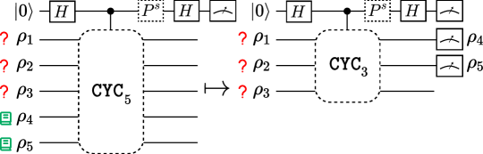
Figure 1: Main result. Quantum circuits for estimating multivariate traces—expressed as $\Delta_{n}(\pmb{\varrho})=\text{Tr}[\rho_{1}\ldots\rho_{n}]=\text{Tr}[\mathtt{CYC}_{n}(\rho_{1}\otimes\ldots\otimes\rho_{n})]$ where $\mathtt{CYC}_{n}$ is a unitary—such as the cycle test [17] typically assume that all input states are either fully unknown (e.g., black-box preparations) or need to be physically prepared on demand. We show that if classical descriptions of $m\leq\lfloor n/2\rfloor$ of these states are available, one can trade the cost of preparing those $m$ states for the cost of measurement and classical post-processing. This substitution relaxes the circuit requirements for estimating such invariants. The figure shows the case of $n=5$ and $m=2$.

The results of Chiribella et al. [69] demonstrate that the swap test can be employed to estimate $\text{Tr}[\rho_{1}A\rho_{2}B]$. Motivated by this, a natural question is whether variations of the destructive swap test [70]—without auxiliary qubits or Fredkin gates—can also be a useful alternative to estimate such multivariate traces in some regimes. Here, we focus on the simplest case of third-order invariants for single-qubit states. We show that it is possible to estimate third-order invariants using circuit variations of a destructive swap test. Nevertheless, we argue that this approach is impractical. While we present a scheme for estimating these invariants given classical state information of one of the three states, the excessive number of required measurements and post-processing renders it useless compared to standard methods or simply performing state tomography.

Although measurement-enhanced versions of destructive tests may not be useful, we are motivated by the goal of estimating invariants destructively. We therefore discuss how to implement destructive cycle tests, which avoid the need for auxiliary qubits to estimate Bargmann invariants, and present a quantum circuit implementation of a destructive 3-cycle test for estimating any third-order Bargmann invariant.

Outline. The remainder of this work is structured as follows. Sec. II presents background on standard tests for estimating Bargmann invariants. It begins with well known schemes for estimating second-order invariants in Sec. II.1, followed by higher-order invariants in Sec. II.2. Section II.3 presents the results by Chiribella et al. [69], which we later generalize in Sec. III. We dub our generalized protocol the measurement-enhanced cycle test, encompassing the standard cycle test scheme, the swap test scheme, and the protocol from Ref. [69] as as specific instances. Section IV investigates if improvements are possible by considering variations of the so-called destructive swap test. In that section we show how to use the destructive swap test to estimate third-order invariants, describe how to implement destructive cycle tests, and present a quantum circuit for estimating third-order invariants. Finally, Sec. V concludes with a discussion of our results, applications, and future directions.

II Background

II.1 Quantum circuits for measuring two-state overlaps

Starting with quantum circuits used to estimate $\text{Tr}[\rho\sigma]$, we first review the swap test [71, 72]. Let us denote by $\mathtt{SWAP}:\mathcal{H}\otimes\mathcal{H}\to\mathcal{H}\otimes\mathcal{H}$ the swap unitary operation such that $\mathtt{SWAP}(\ket{u}\otimes\ket{v})=\ket{v}\otimes\ket{u}$, for every $\ket{u},\ket{v}\in\mathcal{H}$. Given a basis $\{|i\rangle\}_{i}$ for $\mathcal{H}$ we can write the swap unitary as

$$\mathtt{SWAP}=\sum_{i,j}|i\rangle\langle j|\otimes|j\rangle\langle i|,$$

from which it is elementary to show that for general density matrices $\rho_{1},\rho_{2}\in\mathcal{D}(\mathcal{H})$ it holds that

$$\text{Tr}[\rho_{1}\rho_{2}]=\text{Tr}[\mathtt{SWAP}(\rho_{1}\otimes\rho_{2})].$$ (3)

It is then possible to use this relation to propose a quantum circuit for estimating the two-state overlap, known as the swap test [72]. This test performs an Hadamard test [73] where the unitary $U=\mathtt{SWAP}$. When necessary, to specify that we swap systems $\mathcal{H}_{a}$ and $\mathcal{H}_{b}$, we will also write $\mathtt{SWAP}_{a,b}$. The swap test was recently re-discovered by employing machine learning techniques [74, 75] and is illustrated in Fig. 2. For a generalization of this test to multi-qudit systems $\mathcal{H}=(\mathbb{C}^{d})^{\otimes n}$ or to infinite dimensional systems, we refer the reader to Refs. [76, 77, 78, 77].

As can be seen in Fig. 2, to estimate the two-state overlap using the swap test we perform measurements in the auxiliary qubit, leaving the other systems unmeasured. Therefore, the product state $\rho_{1}\otimes\rho_{2}$ is then projected onto another quantum state without being destroyed in the process. Contrastingly, the destructive swap test [70, 29, 18] requires no auxiliary qubit, and uses the fact that the swap operator can be expended in the Bell basis. Therefore, the destructive swap test estimates $\text{Tr}[\rho_{1}\rho_{2}]$ by making a Bell measurement on the bipartite system. The quantum circuit implementation is shown in Fig. 3.

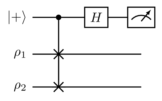
Figure 2: Circuit implementing a swap test. The inputs are two quantum states and an auxiliary qubit system (also known as a control system) that is put in a coherent state $|+\rangle\langle+|\otimes\rho_{1}\otimes\rho_{2}$. A controlled swap (also known as a Fredkin gate) between the auxiliary qubit and the two states is performed. an Hadamard gate is applied to the auxiliary qubit that is then measured in the $Z$ basis $\{|0\rangle,|1\rangle\}$. The two-state overlap is recovered via the relation $p(0)=(1+\text{Tr}[\rho_{1}\rho_{2}])/2$.

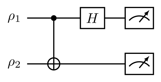
Figure 3: Circuit implementing a destructive swap test. The input state is $\rho_{1}\otimes\rho_{2}$. One then performs a Bell measurement, which is implemented by a CNOT followed by an Hadamard on the first system, and local $Z$ measurements. Assuming each system is a single qubit, the two-state overlap is recovered via the relation $p(1,1)={(1-\text{Tr}[\rho_{1}\rho_{2}])}/{2}$. For generic multi-qubit systems see Ref. [29].

For both tests shown in Figs. 2 and 3 we can imagine that a form of delegated quantum computation is happening, where we do not have complete information of the quantum states that are sent to us by another party. We can perform the quantum computation for this party and return to them the value $\text{Tr}[\rho_{1}\rho_{2}]$ we infer without ever knowing the actual states they prepared.

II.2 Quantum circuits for measuring Bargmann invariants

It is possible to generalize the argument made for the swap test in order to estimate higher-order Bargmann invariants with different implementations of an Hadamard test. We follow Refs. [17, 68]. We start noticing that, for every $n$-tuple of quantum states $\pmb{\varrho}\in\mathcal{D}(\mathcal{H})^{n}$, we can write (1) as

$$\Delta_{n}(\pmb{\varrho})=\text{Tr}[\mathtt{CYC}_{n}(\rho_{1}\otimes\rho_{2}\otimes\ldots\otimes\rho_{n})],$$ (4)

where $\mathtt{CYC}_{n}$ is a unitary associated to the action of a cyclic permutation of $n$ elements

$$(a_{1},a_{2},a_{3}\ldots,a_{n-1},a_{n})\stackrel{{\scriptstyle C_{n}}}{{\mapsto}}(a_{2},a_{3},\ldots,a_{n-1},a_{n},a_{1}).$$ (5)

When $n=2$ we have that $\mathtt{CYC}_{2}\equiv\mathtt{SWAP}$, and we recover Eq. (3). For $n\geq 3$, we know that $\Delta_{n}(\pmb{\varrho})\in\mathbb{C}$ [64]. We can estimate $\Delta_{n}(\varrho)$ using an Hadamard test for which $U=\mathtt{CYC}_{n}$. This type of test is known as the cycle test [17].

Different instances of the cycle test [17] consider different decompositions of $\mathtt{CYC}_{n}$ into different elementary gates. A possible choice is via the sequence of swap unitaries,

$$\mathtt{CYC}_{n}=\mathtt{SWAP}_{n-1,n}\ldots\mathtt{SWAP}_{2,3}\mathtt{SWAP}_{1,2}.$$ (6)

This leads to the circuit implementation of the cycle test shown in Fig. 4. Note that when $n=2$ this reduces to the swap test from Fig. 4.

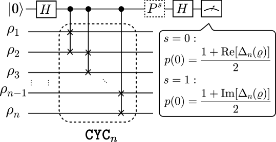
Figure 4: Circuit implementing a cycle test. We show an instance of an Hadamard test, where the unitary $\mathtt{CYC}_{n}$ is the unitary representation of a cyclic permutation $C_{n}$ of $n$ symbols. We initialize a quantum memory of $n+1$ systems in a product state. The first wire in the circuit represents a single qubit system. The remaining wires represent systems of dimension $d\geq 2$. After the controlled cycle operation a gate $P^{s}=\text{diag}(1,i^{s})$ is applied to the auxiliary qubit, later measured with the computational basis. When $s=0$, measuring the auxiliary qubit yields the real part of the Bargmann invariant, while when $s=1$ the imaginary part.

Depending on how the $n$-cycle unitary operator $\mathtt{CYC}_{n}$ is decomposed into SWAPs (or other unitary gates), each such decomposition yields a different quantum circuit capable of estimating Bargmann invariants. One way of improving the depth of the quantum circuit just described is by using entangled states as auxiliary systems, instead of a single-qubit control system as in Fig. 4. We refer to Refs. [17, 68] for details.

So far, all the quantum circuits considered for estimating Bargmann invariants allow for the possibility that all the quantum states in $\pmb{\varrho}$ are provided by another party. In this way, it is natural that the circuits to estimate Bargmann invariants of $n$ unknown quantum states requires $n$ systems to be available as a quantum memory to be used in the quantum computation.

However, as recently shown in Ref. [69], it is possible to estimate third and fourth-order Bargmann invariants using just the swap test circuit from Fig. 2. They do not explicitly consider this specific use as they focus on the estimation of weak values [31, 79, 33]. Yet, it is trivial to see that their protocol can be used for this purpose. Intriguingly, this allows one to use a quantum circuit with two systems (and an additional single qubit auxiliary system) to estimate Bargmann invariants of order up to four. This gain is not only in the accessible memory, but also in the number of necessary Fredkin gates required as a standard cycle test to estimate a fourth-order invariant would need three Fredkin gates. The key insight here is that these circuits require classical information on two of the four states. In what follows, we briefly review the results from Ref. [69].

II.3 The measurement protocol by Chiribella et al.

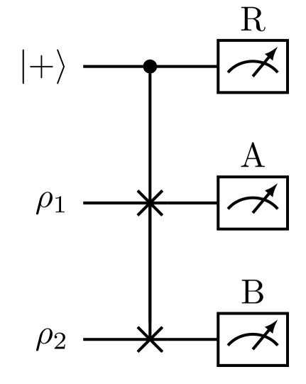
Figure 5: Quantum circuit considered by Chiribella et al. [69]. The input state is $|+\rangle\langle+|\otimes\rho_{1}\otimes\rho_{2}$. The first wire represents a single qubit system, while the remaining wires represent generic single qudit systems. We apply a Fredkin gate between all three systems and perform local measurements. The auxiliary qubit is measured with the positive operator-valued measure (POVM) $R$ from Eq. (7). The other systems are measured with generic POVMs $A$ and $B$. We dub this a measurement-enhanced swap test since the measurements of $A,\,B$ allow for the estimation of $\text{Tr}[\rho_{1}A\rho_{2}B]$, otherwise inaccessible to the standard swap test—hence the ‘enhancement’ in the order of the accessible multivariate trace.

The relevant quantum circuit is shown in Fig. 5. From it, Ref. [69] shows how to estimate $\text{Tr}[\rho_{1}A\rho_{2}B]$, where $A$ and $B$ are positive operator-valued measures (POVMs) [80]. Suppose we have access to a tripartite system $\mathcal{H}_{C}\otimes\mathcal{H}_{S_{1}}\otimes\mathcal{H}_{S_{2}}\equiv\mathbb{C}^{2}\otimes\mathcal{H}\otimes\mathcal{H}$, where $\mathcal{H}$ is an arbitrary finite dimensional Hilbert space. The system $\mathcal{H}_{C}=\mathbb{C}^{2}$ is our control (or auxiliary) qubit. The algorithm proceeds as follows:

1. Prepare a tripartite product state $|+\rangle\langle+|\otimes\rho_{1}\otimes\rho_{2}$, where $|+\rangle=\nicefrac{{1}}{{\sqrt{2}}}(|0\rangle+|1\rangle)\in\mathbb{C}^{2}$, while $\rho_{1},\rho_{2}\in\mathcal{D}(\mathcal{H})$ are generic.

2. Apply the controlled $\mathtt{SWAP}$ gate, that we denote as $\mathtt{cSWAP}$ .

3. Measure system $\mathcal{H}_{S_{1}}$ with a POVM $A=\{P_{j}\}_{j}$.

4. Measure system $\mathcal{H}_{S_{2}}$ with a POVM $B=\{Q_{k}\}_{k}$.

5. Measure the auxiliary qubit system $\mathcal{H}_{C}$ with a POVM $\{R_{c}\}_{c=0}^{3}$ given by

   $$R_{0} =\frac{1}{2}|+\rangle\langle+|, R_{1} =\frac{1}{2}|-\rangle\langle-|,$$

   $$R_{2} =\frac{1}{2}|+_{i}\rangle\langle+_{i}|, R_{3} =\frac{1}{2}|-_{i}\rangle\langle-_{i}|,$$ (7)

   where $|\pm\rangle=\nicefrac{{1}}{{\sqrt{2}}}(|0\rangle\pm|1\rangle)$ and $|\pm_{i}\rangle=\nicefrac{{1}}{{\sqrt{2}}}(|0\rangle\pm i|1\rangle)$.

From this protocol, one obtains the following joint distribution:

$$p(j,k,c|\rho_{1},\rho_{2})=$$

$$=\text{Tr}[(P_{j}\otimes Q_{k}\otimes R_{c})\,\mathtt{cSWAP}(\rho_{1}\otimes\rho_{2}\otimes|+\rangle\langle+|)\mathtt{cSWAP}^{\dagger}].$$

As shown by Ref. [69], sampling from this distribution allows us to learn the real and imaginary part of the complex values

$$q(j,k|\rho_{1},\rho_{2}):=\text{Tr}[P_{j}\rho_{1}Q_{k}\rho_{2}].$$

To see this, let us consider for simplicity the case where $B=\mathbb{1}$. In this case, the joint distribution simplifies to

$$p(j,c|\rho_{1},\rho_{2}) =\frac{1}{8}\Bigr{(}\text{Tr}[P_{j}\rho_{1}]+\text{Tr}[P_{j}\rho_{2}]$$

$$+2\theta(1-c)(-1)^{c}\text{Re}[\text{Tr}[P_{j}\rho_{1}\rho_{2}]]$$

$$-2\theta(c-2)(-1)^{c}\text{Im}[\text{Tr}[P_{j}\rho_{1}\rho_{2}]]\Bigr{)},$$ (8)

where $\theta(t)$ is the Heaviside step function [69, Eq.(10), Appendix A] and $c\in\{0,1,2,3\}$. We will generalize these results later in Sec. III.

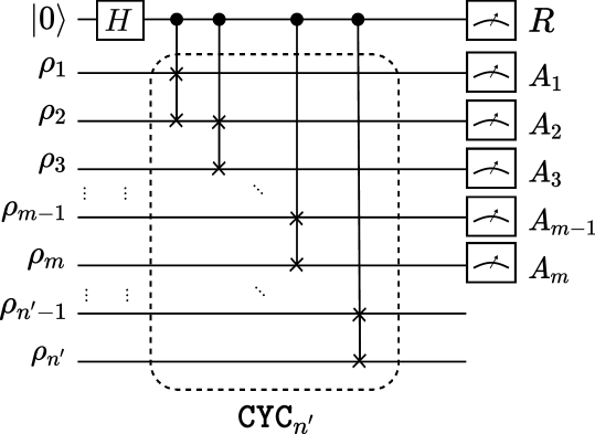
Figure 6: Circuit implementing a measurement-enhanced cycle test. The number of unknown $d$-dimensional quantum states is $n^{\prime}$ and the number of known states is $m\leq n^{\prime}$. The order of the estimated multivariate trace is $n=n^{\prime}+m$. Up to the measurements, the circuit is the same as the one we show in Fig. 4. We perform the POVM measurement $R$ on the auxiliary qubit (see Eq. (7)) and local measurements to $m\leq n^{\prime}$ systems using the POVMs $A_{1},\,\ldots,\,A_{m}$.

Note that in this case estimating this quantity has different demands in terms of prior knowledge of its constituents. While the quantum states $\rho_{1},\rho_{2}\in\mathcal{D}(\mathcal{H})$ can be completely unknown by who implements the quantum circuit, the operators $P_{j},Q_{k}$ must be known. We shall refer to this quantum algorithm as a measurement-enhanced swap test, as it allows us to estimate more than just two-state overlaps (hence the ‘enhancement’) given that we can perform the measurements $A,\,B$. Specifically, we can see that if $A=\{\rho_{3},\mathbb{1}-\rho_{3}\}$ and $B=\mathbb{1}$ we have that the resulting construction shown above for $p(j,c|\rho_{1},\rho_{2})$ becomes

$$p(\rho_{3},0)=\frac{1}{8}\Bigr{(}\text{Tr}[\rho_{1}\rho_{3}]+\text{Tr}[\rho_{2}\rho_{3}]+2\text{Re}[\text{Tr}[\rho_{1}\rho_{2}\rho_{3}]]\Bigr{)},$$

where we have let $P_{j}\equiv\rho_{3}$, $c=0$, and $p(\rho_{3},0)\equiv p(\rho_{3},0|\rho_{1},\rho_{2})$. Hence we conclude that we can learn from this estimation the real part of the third-order Bargmann invariant. Letting $c>2$ allows us to infer the imaginary part of the third-order invariant. In what follows, we will generalize the protocol introduced by Ref. [69], and then discuss how one can use it to measure multivariate traces of states.

III Measurement-enhanced
cycle test

Fix $n\in\mathbb{N}$ to be any integer greater than or equal to $2$. Our goal is to estimate a Bargmann invariant $\text{Tr}[\rho_{1}\ldots\rho_{n}]$ of order $n$. The number of unknown $d$-dimensional quantum states entering the quantum circuit is $n^{\prime}\leq n$, and we denote them as the tuple $\pmb{\varrho}=(\rho_{1},\ldots,\rho_{n^{\prime}})$, while the number of quantum states for which we have classical tomographic information is $0\leq m\leq n^{\prime}$ such that $n^{\prime}+m=n$, and we denote this as the tuple $\widetilde{\pmb{\varrho}}=(\widetilde{\rho}_{1},\ldots,\widetilde{\rho}_{m})$. As we have done previously, we will next introduce how to estimate multivariate traces of states and observables using a generalization of the protocol introduced by Chiribella et al. and then show how the estimation of Bargmann invariants is a particular instance. In what follows, the $d$-dimensional quantum systems have any finite dimension, and only the auxiliary system is taken to be a single-qubit system.

We start by considering a generalization of the quantum circuit from Fig. 5. Instead of the $\mathtt{cSWAP}$ considered in Fig. 5 we let the controlled unitary to be $\mathtt{cCYC}_{n}$, i.e. a controlled operation of the unitary $\mathtt{CYC}_{n}$. We show one possible implementation of such controlled unitary in Fig. 4. Letting $\varrho:=\rho_{1}\otimes\rho_{2}\otimes\ldots\otimes\rho_{n^{\prime}}$ to be the input system on our circuit, the first operation performed is as follows

$$|+\rangle\langle+|\otimes\varrho\longmapsto\mathtt{cCYC}_{n^{\prime}}(|+\rangle\langle+|\otimes\varrho)\mathtt{cCYC}_{n^{\prime}}^{\dagger},$$ (9)

where

$$\mathtt{cCYC}_{n^{\prime}}=|0\rangle\langle 0|\otimes\mathbb{1}+|1\rangle\langle 1|\otimes\mathtt{SWAP}_{n^{\prime},n^{\prime}-1}\ldots\mathtt{SWAP}_{12}.$$ (10)

This leaves the entire system in the state

$$\frac{1}{2}|0\rangle\langle 0|\otimes\varrho+\frac{1}{2}|1\rangle\langle 1|\otimes\mathtt{CYC}_{n^{\prime}}(\varrho)+$$

$$+\frac{1}{2}\Bigr{(}|0\rangle\langle 1|\otimes\sum_{\mathbf{a}}p_{\mathbf{a}}|a_{2}\rangle\langle a_{1}|\otimes\ldots\otimes|a_{1}\rangle\langle a_{n^{\prime}}|+\mathrm{h.\,c.}\Bigr{)},$$

where $\mathbf{a}=(a_{1},a_{2},\ldots,a_{n^{\prime}})$ is a multi-index label which we use as $\sum_{\mathbf{a}}\equiv\sum_{a_{1},a_{2},\ldots,a_{n^{\prime}}}$. Moreover $p_{\mathbf{a}}=p_{a_{1}}^{1}p_{a_{2}}^{2}\ldots p_{a_{n^{\prime}}}^{n^{\prime}}$ is the product statistics, and we have written each state $\rho_{i}$ in terms of some—not necessarily known—convex combination of pure quantum states $\rho_{i}=\sum_{a_{i}}p_{a_{i}}^{i}|a_{i}\rangle\langle a_{i}|.$ We have also used

$$\mathtt{CYC}_{n^{\prime}}(|a_{1},a_{2},\ldots,a_{n^{\prime}}\rangle) =|a_{2},\ldots,a_{n^{\prime}},a_{1}\rangle.$$

If we stop here, measuring the auxiliary qubit in the $X$ ($Y$) basis performs the cycle test operation for estimating the real (imaginary) part of a $n^{\prime}$-th order Bargmann invariants [17, 35]. Now let us assume that not only the control qubit is measured on the $X$ basis, but also the first $m\leq n^{\prime}$ systems, for some fixed value $m$, are measured with respect to POVMs $A_{1}=\{P_{j_{1}}\}_{j_{1}}$, $\ldots$, $A_{m}=\{P_{j_{m}}\}_{j_{m}}$. This yields a joint probability distribution

$$p(j_{1},\ldots,j_{m},\pm) = \frac{1}{4}\Bigl{(}\prod_{i=1}^{m}\operatorname{Tr}[P_{j_{i}}\rho_{i}]+\prod_{i=1}^{m}\operatorname{Tr}[P_{j_{i}}\rho_{i+1}]\pm\sum_{\mathbf{a}}p_{\mathbf{a}}\langle a_{2}|P_{j_{1}}|a_{1}\rangle\langle a_{3}|P_{j_{2}}|a_{2}\rangle\ldots\langle a_{m+1}|P_{j_{m}}|a_{m}\rangle\times$$

$$\times \langle a_{m+2}|a_{m+1}\rangle\ldots\langle a_{n^{\prime}}|a_{n^{\prime}-1}\rangle\langle a_{1}|a_{n^{\prime}}\rangle\pm\mathrm{c.\,c.}\Bigr{)}$$

$$= \frac{1}{4}\Bigl{(}\prod_{i=1}^{m}\operatorname{Tr}[P_{j_{i}}\rho_{i}]+\prod_{i=1}^{m}\operatorname{Tr}[P_{j_{i}}\rho_{i+1}]\pm\sum_{\mathbf{a}}p_{\mathbf{a}}\langle a_{1}|a_{n^{\prime}}\rangle\langle a_{n^{\prime}}|a_{n^{\prime}-1}\rangle\ldots\langle a_{m+2}|a_{m+1}\rangle\times$$

$$\times \langle a_{m+1}|P_{j_{m}}|a_{m}\rangle\ldots\langle a_{3}|P_{j_{2}}|a_{2}\rangle\langle a_{2}|P_{j_{1}}|a_{1}\rangle\pm\mathrm{c.\,c.}\Bigr{)}$$

$$= \frac{1}{4}\Bigl{(}\prod_{i=1}^{m}\operatorname{Tr}[P_{j_{i}}\rho_{i}]+\prod_{i=1}^{m}\operatorname{Tr}[P_{j_{i}}\rho_{i+1}]\pm 2\operatorname{Re}[\operatorname{Tr}(\rho_{n^{\prime}}\ldots\rho_{m+2}\rho_{m+1}P_{j_{m}}\rho_{m}P_{j_{m-1}}\rho_{m-1}\ldots P_{j_{2}}\rho_{2}P_{j_{1}}\rho_{1})]\Bigr{)}.$$

To simplify the notation we write $\mathbf{j}=(j_{1},j_{2},\ldots,j_{m})$, and we also denote

$$\square_{n^{\prime}+m}(\mathbf{j},\pmb{\varrho}):=\operatorname{Tr}(\rho_{n^{\prime}}\ldots\rho_{m+1}P_{j_{m}}\rho_{m}\ldots P_{j_{1}}\rho_{1}).$$ (11)

Note that the above is not a Bargmann invariant, since each $P_{j_{m}}$ is not necessarily a quantum state, but a generic POVM element (hence the different notation of using $\square$ instead of $\Delta$) .

Instead of performing an $X$ measurement of the auxiliary qubit, we can perform random measurements with respect to both $X$ and $Y$ bases on the auxiliary (control) qubit, using the four outcome POVM $R$ from Eq. (7). In this case, the joint probability distribution becomes:

$$p(\mathbf{j},c) =\frac{1}{8}\Bigl{(}\prod_{i=1}^{m}\operatorname{Tr}[P_{j_{i}}\rho_{i}]+\prod_{i=1}^{m}\operatorname{Tr}[P_{j_{i}}\rho_{i+1}]$$

$$+2\theta(1-c)(-1)^{c}{\rm Re}\left[\square_{n^{\prime}+m}(\mathbf{j},\pmb{\varrho})\right]$$

$$-2\theta(c-2)(-1)^{c}{\rm Im}\left[\square_{n^{\prime}+m}(\mathbf{j},\pmb{\varrho})\right]\Bigr{)},$$

where we have used $\theta(t)$ to denote the Heaviside step function, and $c\in\{0,1,2,3\}$ denotes the outcomes from the POVM measurement $R=\{R_{c}\}_{c}$ of the auxiliary qubit. The above generalizes the construction considered in Ref. [69], that was reviewed in Sec. II.3. Specifically, we recover Eq. (8) by making $m=1$ and $j_{1}\equiv j$.

If we have $m$ observables $A_{m}$ with the corresponding POVM decompositions

$$A_{m}=\sum_{j}x_{j_{m}}P_{j_{m}},$$ (12)

we can define a random variable $\tilde{X}$ that takes values

$$\widetilde{x}_{j_{1},\ldots,j_{m},c}:=2x_{j_{1}}\ldots x_{j_{m}}\,(-1)^{c}\,\Big{[}\,\theta(1-c)-i\theta(c-2)\Big{]}$$ (13)

with respect to the probability distribution $p(\mathbf{j},c)$. Note that the values $x_{j_{i}}$ are given by Eq. (12). The expectation value of $\tilde{X}$ returns the value of $\square_{n^{\prime}+m}({\mathbf{j}},\pmb{\varrho})$ since

$$\mathbb{E}[\tilde{X}]=$$

$$=\sum_{j_{1},\ldots,j_{m},c}2\prod_{i=1}^{m}x_{j_{i}}\,(-1)^{c}\,\Big{[}\,\theta(1-c)-i\theta(c-2)\Big{]}p(\mathbf{j},c)$$ (14)

$$=\sum_{j_{1},\ldots,j_{m}}x_{j_{1}}\ldots x_{j_{m}}\Bigl{(}{\rm Re}[\square_{n}({\mathbf{j}},\pmb{\varrho})]+i{\rm Im}[\square_{n}({\mathbf{j}},\pmb{\varrho})]\Bigr{)}$$ (15)

$$=\sum_{j_{1},\ldots,j_{m}}x_{j_{1}}\ldots x_{j_{m}}\square_{n}({\mathbf{j}},\pmb{\varrho}).$$ (16)

Above, we have used that $n=n^{\prime}+m$. The terms having products of traces $\text{Tr}[P_{j_{i}}\rho_{i}]$ cancel out going from Eq. (14) to Eq. (15) due to the sum in $c$, since we get a sum of contributions $(-1)^{0}+(-1)^{1}+i((-1)^{2}+(-1)^{3})=1-1+i-i=0$. This means that Eq. (16) guarantees we can estimate a quantity $\square_{n^{\prime}+m}({\mathbf{j}},\pmb{\varrho})$ given by Eq. (11) by sampling from the distribution generated by performing controlled SWAPs on $n^{\prime}$ systems and measuring observables $\{A_{i}\}_{i=1}^{m}$ on $m\leq n^{\prime}$ of these systems. We remark that (see for instance Refs. [69, 35, 68]) estimating such traces is exponentially better (in sample complexity) than performing quantum state tomography of all unknown quantum states $n^{\prime}$.

We now conclude by applying our test to the estimation of Bargmann invariants. We do so by restricting the POVMs to be such that $A_{i}=\{\widetilde{\rho}_{i},\mathbb{1}-\widetilde{\rho}_{i}\}$. In this case, selecting the specific case where the labels satisfy $(P_{j_{1}},\ldots,P_{j_{m}})=(\widetilde{\rho}_{1},\ldots,\widetilde{\rho}_{m})\equiv\widetilde{\pmb{\varrho}}$ we end up with

$$\Delta_{n^{\prime}+m}(\widetilde{\pmb{\varrho}},\pmb{\varrho})=\Tr[\rho_{n^{\prime}}\ldots\rho_{m+2}\rho_{m+1}\widetilde{\rho}_{m}\rho_{m}\ldots\widetilde{\rho}_{1}\rho_{1}].$$ (17)

This means that any $n$-th order Bargmann invariant can be estimated by using a cyclic shift on $n^{\prime}\leq n$ quantum states (hence, $n^{\prime}-1$ controlled SWAPs) and measurements on $m\leq n^{\prime}$ systems where $n=n^{\prime}+m$. Alternatively, at least $\lceil n/2\rceil$ systems and one auxiliary qubit, and hence $\lceil n/2\rceil-1$ controlled SWAPs, are necessary to estimate $n$-th order Bargmann invariants using our sampling protocol and the decomposition of $\mathtt{CYC}_{n}$ as by Eq. (6). Hence, the sampling protocol requires only half of systems and controlled SWAPs compared with the original cycle test protocol of Refs. [17, 35].

IV Destructive tests for estimating Bargmann invariants

So far, we have considered the situation where we have generalized the cycle test to include classical information of observables and investigated how this allows us to access information of higher order multivariate traces. It is natural to ask whether the destructive swap test can also be generalized to estimate invariants (1) of order larger than $n=2$, provided we have access to prior classical tomographic information of some of the states.

While in the last section the states in $\pmb{\rho}$ where taken to be generic quantum states on a finite-dimensional Hilbert space, i.e. $\pmb{\rho}\in\mathcal{D}(\mathbb{C}^{d})^{n}$, in this section we restrict to the case where $d=2$, i.e., every state in the tuple is a single-qubit quantum state.

We start by discussing how a third-order Bargmann invariant can be estimated under certain assumptions on prior knowledge on the corresponding states using instances of a deterministic swap test. First, we notice that every third-order Bargmann invariant is quantum realizable by single qubit pure quantum states [64]. Therefore, without loss of generality, we consider $|\psi_{1}\rangle,|\psi_{2}\rangle,|\widetilde{\psi}_{3}\rangle\in\mathbb{C}^{2}$ to be pure single-qubit states, where $|\psi_{1}\rangle$ and $|\psi_{2}\rangle$ are not necessarily known. The corresponding third-order Bargmann invariant is given by:

$$\Delta_{3}(\psi_{1},\psi_{2},\widetilde{\psi}_{3})=\langle\psi_{1}|\psi_{2}\rangle\langle\psi_{2}|\widetilde{\psi}_{3}\rangle\langle\widetilde{\psi}_{3}|\psi_{1}\rangle,$$ (18)

where we use the notation $\psi_{i}:=|\psi_{i}\rangle\langle\psi_{i}|$ for pure states in the argument of Bargmann invariants.

On the other hand, taking into account the unitary-invariance of Bargmann invariants [18], for any triplet $|\psi_{1}\rangle,|\psi_{2}\rangle,|\tilde{\psi}_{3}\rangle\in\mathbb{C}^{2}$ we can always find some unitary $U$ such that $U|\tilde{\psi}_{3}\rangle=|0\rangle$ using the available tomographic classical information of $|\tilde{\psi}_{3}\rangle$. In this case,

$$\Delta_{3}(\psi_{1},\psi_{2},\widetilde{\psi}_{3}) =\langle\psi_{1}|U^{\dagger}U|\psi_{2}\rangle\langle\psi_{2}|U^{\dagger}|0\rangle\langle 0|U|\psi_{1}\rangle$$

$$:=\langle\psi_{U}|\phi_{U}\rangle\langle\phi_{U}|0\rangle\langle 0|\psi_{U}\rangle$$

$$=\Delta_{3}(\psi_{U},\phi_{U},0),$$

where $|\psi_{U}\rangle=U|\psi_{1}\rangle$, and $|\phi_{U}\rangle=U|\psi_{2}\rangle$. Therefore, given access to tomographic classical information of $|\tilde{\psi}_{3}\rangle$, estimation of a generic Bargmann invariant (18) is equivalent to estimation of Bargmann invariant on the triplet $U|\psi_{1}\rangle$, $U|\psi_{2}\rangle$, and $|0\rangle$.

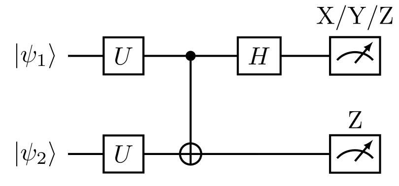
Figure 7: Circuit implementing a modified destructive swap test for the estimation of third order Bargmann invariants. The input state is $|\psi_{1}\rangle\otimes|\psi_{2}\rangle$. One then applies a unitary operator $U$ defined as $U|\widetilde{\psi}_{3}\rangle=|0\rangle$, followed by a combination of CNOT and Hadamard gates similarly to destructive swap test. Finally, the second qubit undergoes a $Z$ measurement, while the first qubit is measured in $X$-, $Y$-, or $Z$-basis. Assuming each system is a single qubit, the third order Bargmann invariant is given by Eq. (25).

Notice that the projector $|0\rangle\langle 0|$ can be decomposed into operators $\frac{1}{2}(\mathbb{1}\pm Z)$, where $Z$ is the Z-Pauli operator. Therefore, we can write

$$\Delta_{3}(\psi_{1},\psi_{2},\widetilde{\psi}_{3}) = \frac{1}{2}\Bigl{(}\Delta_{2}(\psi_{U},\phi_{U})+\chi(\psi_{U},\phi_{U})\Bigr{)},$$

where $\chi(\psi_{U},\phi_{U}):=\langle\psi_{U}|\phi_{U}\rangle\langle\phi_{U}|Z|\psi_{U}\rangle$. Since $\Delta_{2}(\psi_{U},\phi_{U})$ can be estimated via the destructive swap test discussed in Sec. II.1, the core challenge lies in estimation of $\chi(\psi_{U},\phi_{U})$. This can be achieved using the quantum circuit shown in Fig. 3, where, in contrast to estimation of second order Bargmann invariant, only the second qubit is measured in computational basis, while the first qubit is measured in $X$- and $Y$-basis in order to obtain its real and imaginary parts, respectively. In order to proof this, we take into account that, decomposing the states as | $\psi_{U}\rangle=a|0\rangle+a^{\prime}|1\rangle$ and $|\phi_{U}\rangle=b|0\rangle+b^{\prime}|1\rangle$, with $|a|^{2}+|a^{\prime}|^{2}=1$ and $|b|^{2}+|b^{\prime}|^{2}=1$, we can write

$$\chi(\psi_{U},\phi_{U})=|a|^{2}|b|^{2}-|a^{\prime}|^{2}|b^{\prime}|^{2}+2i\mathrm{Im}[ab^{*}a^{\prime*}b^{\prime}].$$ (19)

On the other hand, the circuit in Fig. 3 produces a state

$$|\Psi\rangle=\frac{1}{\sqrt{2}}\Biggl{(}|0\rangle\Bigl{(}(ab+a^{\prime}b^{\prime})|0\rangle+(ab^{\prime}+a^{\prime}b)|1\rangle\Bigr{)}$$

$$+|1\rangle\Bigl{(}(ab-a^{\prime}b^{\prime})|0\rangle+(ab^{\prime}-a^{\prime}b)|1\rangle\Bigr{)}\Biggr{)}.$$ (20)

before performance of local measurements. Then, a straightforward calculation shows that a measurement of the first qubit in $X$-basis and the second qubit in computational basis yields the probabilities

$$p(+,0) = |a|^{2}|b|^{2},$$ (21)

$$p(-,0) = |a^{\prime}|^{2}|b^{\prime}|^{2},$$ (22)

while measuring the first qubit in the $Y$-basis provides

$$p(\pm_{i},1)=|a|^{2}|b^{\prime}|^{2}+|a^{\prime}|^{2}|b|^{2}\mp\mathrm{Im}[ab^{*}a^{\prime*}b^{\prime}],$$ (23)

where $p(\pm,0)$ and $p(\pm_{i},1)$ are the corresponding probabilities of finding the qubits in states $|\pm\rangle\otimes|0\rangle$ and $|\pm_{i}\rangle\otimes|1\rangle$, respectively. Therefore, we conclude that

$$\chi(\psi_{U},\phi_{U})=p(+,0)-p(-,0)-i\Bigl{(}p(+_{i},1)-p(-_{i},1)\Bigr{)},$$ (24)

In turn, measuring both qubits in computational basis recovers destructive swap test discussed in Sec. II.1. Therefore, taking into account unitary invariance of Bargmann invariants, we conclude that the third order Bargmann invariant can be estimated by

$$\Delta_{3}(\psi_{1},\psi_{2},\widetilde{\psi}_{3}) =\frac{1}{2}\Bigl{(}1-2p(1,1)+p(+,0)$$

$$-p(-,0)-i\Bigl{(}p(+_{i},1)-p(-_{i},1)\Bigr{)}\Bigr{)}.$$ (25)

We observe that a destructive cycle test can be introduced to estimate Bargmann invariants and to explore potential measurement-enhanced variants. Although the analysis of the destructive swap test suggests that such enhancements may offer limited benefit, destructive cycle tests—extending the swap test case from Fig. 3—may still be of independent interest. Motivated by this, we now show that, in principle, a generic destructive cycle test can be described in a conceptually straightforward manner. Due to Eq. (4), $n$-th order Bargmann invariants for a tuple of states $\pmb{\varrho}=(\rho_{1},\ldots,\rho_{n})$ can be seen as expectation values of the $n$-cycle unitary operator $\mathtt{CYC}_{n}$ with respect to the state $\varrho=\rho_{1}\otimes\ldots\otimes\rho_{n}$,

$$\Delta_{n}(\rho_{1},\ldots,\rho_{n})=\langle\mathtt{CYC}_{n}\rangle_{\varrho}.$$ (26)

Therefore, a destructive cycle test can be constructed using diagonalization of the unitary operator $\mathtt{CYC}_{n}$ with respect to an entangled basis.

Let us consider the case of qubit states $\rho_{1},\ldots,\rho_{n}\in\mathcal{D}(\mathbb{C}^{2})$ and the corresponding total Hilbert space $\mathcal{H}=(\mathbb{C}^{2})^{\otimes n}$. The former can be spanned by computational basis states that form a set $\mathcal{S}_{n}=\{|\mathbf{x}\rangle\}_{\mathbf{x}\in\{0,1\}^{n}}$, where $\mathbf{x}\in\{0,1\}^{n}$ is a string of $n$ bits. Then $\mathcal{H}$ can be decomposed into $n+1$ orthogonal subspaces

$$\mathcal{H}=\bigoplus_{k=0}^{n}\mathcal{H}_{\mathrm{HW}}^{(k)},$$ (27)

where $\mathcal{H}_{\mathrm{HW}}^{(k)}$ are spanned by sets $\mathcal{S}_{n}^{(k)}\subseteq\mathcal{S}_{n}$ of ${n\choose k}$ states $|\mathbf{x}_{k}\rangle$ corresponding to bit strings $\mathbf{x}_{k}$ of fixed Hamming weight $k$, i.e., bit strings with $k$ 1’s. For example, for $n=3$, this decomposition is given by

$$\mathcal{S}_{3}^{(0)} =\{|000\rangle\},$$

$$\mathcal{S}_{3}^{(1)} =\{|001\rangle,|010\rangle,|100\rangle\},$$

$$\mathcal{S}_{3}^{(2)} =\{|110\rangle,|101\rangle,|011\rangle\},$$

$$\mathcal{S}_{3}^{(3)} =\{|111\rangle\}.$$

The operator $\mathtt{CYC}_{n}$ preserves the Hamming weight of computational basis states, hence, it acts invariantly on each subset $\mathcal{S}_{n}^{(k)}$ and corresponding subspace of decomposition in Eq. (27), so that $\mathtt{CYC}_{n}(\mathcal{H}_{\mathrm{HW}}^{(k)})\subseteq\mathcal{H}_{\mathrm{HW}}^{(k)}$. Moreover, each subset $\mathcal{S}_{n}^{(k)}$ can be further decomposed into $c_{k}$ cyclic orbits $\{\mathcal{O}^{(k,m)}_{n}\}_{m=0}^{c_{k}}$ with respect to the action of $\mathtt{CYC}_{n}$. These are equivalence classes $\mathcal{S}_{n}/\sim_{\mathsf{cyc}}$ under an equivalence relation which, for any $|\mathbf{x}_{1}\rangle,|\mathbf{x}_{2}\rangle\in\mathcal{S}_{n}$, is defined as follows:

$$|\mathbf{x}_{1}\rangle\sim_{\mathsf{cyc}}|\mathbf{x}_{2}\rangle\Leftrightarrow\exists j\in\{0,\ldots,n-1\},\;|\mathbf{x}_{1}\rangle=\mathtt{CYC}_{n}^{j},|\mathbf{x}_{2}\rangle.$$ (28)

Therefore, each cyclic orbit can be defined as

$$\mathcal{O}^{(k,m)}_{n} = [|\mathbf{x}\rangle]_{\sim_{\mathsf{cyc}}}=\left\{\mathtt{CYC}_{n}^{j}|\mathbf{x}\rangle\right\}_{j=0}^{r^{(k,m)}_{n}-1},$$ (29)

where $r^{(k,m)}_{n}$ is the size of the cyclic orbit $\mathcal{O}^{(k,m)}_{n}$, i.e., the minimal period such that $\mathtt{CYC}_{n}^{r^{(k,m)}_{n}}\ket{\mathbf{x}}=\ket{\mathbf{x}}$. Therefore, each $\mathcal{H}_{\mathrm{HW}}^{(k)}$ can be further decomposed into $r^{(k,m)}_{n}$-dimensional invariant subspaces spanned by the corresponding cyclic orbits.

For the sake of illustration, while in the case $n=3$ the cyclic orbits $\mathcal{O}^{(k,m)}_{n}$ coincide with entire subsets $\mathcal{S}_{3}^{(k)}$, the case $n=4$ provides a non-trivial decomposition of $\mathcal{S}_{4}^{(k)}$. In particular, the subset $\mathcal{S}_{4}^{(2)}=\{|0011\rangle,|0101\rangle,|0110\rangle,|1001\rangle,|1010\rangle,|1100\rangle\}$ can be split into two cyclic orbits

$$\mathcal{O}_{4}^{(2,0)} =\{|0011\rangle,|0110\rangle,|1100\rangle,|1001\rangle\},$$

$$\mathcal{O}_{4}^{(2,1)} =\{|1010\rangle,|0101\rangle\},$$

of periods $r^{(2,0)}_{4}=4$ and $r^{(2,1)}_{4}=2$, respectively.

The $n$-cycle operator $\mathtt{CYC}_{n}$ can be diagonalized in the basis obtained by using the quantum Fourier transform unitary on each cyclic orbit, defining hence the vectors

$$\ket{\psi^{(k,m)}_{n,\ell}}=\frac{1}{\sqrt{r^{(k,m)}_{n}}}\sum_{j=0}^{r^{(k,m)}_{n}-1}(\omega^{(k,m)}_{n,\ell})^{j}\ket{\mathbf{x}_{n,j}^{(k,m)}},$$

where $\{\ket{\mathbf{x}_{j}^{(k,m)}}\}_{j=0}^{r^{(k,m)}_{n}-1}=\mathcal{O}^{(k,m)}_{n}$, and $\omega^{(k,m)}_{n,\ell}$ is an $r^{(k,m)}_{n}$-th root of unity $\omega^{(k,m)}_{n,\ell}=e^{2\pi i\ell/r^{(k,m)}_{n}}$, with $\ell=0,\ldots,r^{(k,m)}_{n}-1$, associated to the size of the corresponding cyclic orbit $\mathcal{O}^{(k,m)}_{n}$. Then, by construction, these states are eigenstates of the $\mathtt{CYC}_{n}$ with the corresponding eigenvalues $\omega_{\ell}$,

$$\mathtt{CYC}_{n}\ket{\psi^{(k,m)}_{n,\ell}}=\omega^{(k,m)}_{n,\ell}\ket{\psi^{(k,m)}_{n,\ell}},$$

for all $\ell$. The complete set of vectors $\{\ket{\psi^{(k,m)}_{n,\ell}}\}_{\ell,k,m}$ provided by all cyclic orbits describes an orthonormal eigenbasis of $\mathcal{H}=(\mathbb{C}^{2})^{\otimes n}$ with respect to $\mathtt{CYC}_{n}$. Therefore, from Eq. (26), $n$-th order Bargmann invariant can be estimated by preparing $n$ qubits in the product state $\varrho=\rho_{1}\otimes\ldots\otimes\rho_{n}$ and performing the measurements with respect to this eigenbasis:

$$\Delta_{n}(\rho_{1},\ldots,\rho_{n})=\sum_{\ell,k,m}\omega^{(k,m)}_{n,\ell}\text{Tr}\left[\varrho|\psi_{n,\ell}^{(k,m)}\rangle\langle\psi_{n,\ell}^{(k,m)}|\right].$$ (30)

We refer to this method of estimating Bargmann invariants as the destructive cycle test. For concreteness, let us restrict our attention to the case $n=3$. The operator $\mathtt{CYC}_{3}$ is diagonal in the orthonormal basis composed of two product states

$$\ket{\psi_{3,0}^{(0)}}=\ket{000},\quad\ket{\psi_{3,0}^{(3)}}=\ket{111},$$

and six $W$-like states with complex phases

$$\ket{\psi^{(1)}_{3,0}} =\frac{1}{\sqrt{3}}(\ket{001}+\ket{010}+\ket{100}),$$

$$\ket{\psi^{(2)}_{3,0}} =\frac{1}{\sqrt{3}}(\ket{110}+\ket{101}+\ket{011}),$$

$$\ket{\psi^{(1)}_{3,1}} =\frac{1}{\sqrt{3}}(\omega^{2}\ket{001}+\omega\ket{010}+\ket{100}),$$

$$\ket{\psi^{(2)}_{3,1}} =\frac{1}{\sqrt{3}}(\omega^{2}\ket{110}+\omega\ket{101}+\ket{011}),$$

$$\ket{\psi^{(1)}_{3,2}} =\frac{1}{\sqrt{3}}(\omega\ket{001}+\omega^{2}\ket{010}+\ket{100}),$$

$$\ket{\psi^{(2)}_{3,2}} =\frac{1}{\sqrt{3}}(\omega\ket{110}+\omega^{2}\ket{101}+\ket{011}),$$

where $\omega=e^{2\pi i/3}$ is a cube root of unity, and the index $m$ is omitted since, for $n=3$, each subset $\mathcal{S}_{n}^{(k)}$ has a unique cyclic orbit. Therefore,

$$\mathtt{CYC}_{3} =\sum_{k=0}^{3}\Pi_{3,0}^{(k)}+\omega(\Pi_{3,1}^{(1)}+\Pi_{3,1}^{(2)})+\omega^{2}(\Pi_{3,2}^{(1)}+\Pi_{3,2}^{(2)}),$$

where $\Pi_{3,\ell}^{(k)}=|\psi^{(k)}_{3,\ell}\rangle\langle\psi^{(k)}_{3,\ell}|$. This means that $\Delta_{3}(\rho_{1},\rho_{2},\rho_{3})$ can be estimated by preparing three qubits in the product quantum state $\varrho=\rho_{1}\otimes\rho_{2}\otimes\rho_{3}$ and performing a projective measurement in this basis, collecting the corresponding probabilities,

$$\Delta_{3}(\rho_{1},\rho_{2},\rho_{3}) = 1-(1-\omega)(p_{1}^{(1)}+p_{1}^{(2)})$$ (31)

$$- (1-\omega^{2})(p_{2}^{(1)}+p_{2}^{(2)}),$$

where $p_{\ell}^{(k)}=\text{Tr}[(\rho_{1}\otimes\rho_{2}\otimes\rho_{3})\Pi_{3,\ell}^{(k)}]$. Similarly to destructive swap test, due to the cyclic property of trace, measurement in the eigenbasis of $\mathtt{CYC}_{3}$ can be substituted by local measurements in computational basis using unitary transformations defined via $|\psi_{3,\ell}^{(k)}\rangle=U_{3,\ell}^{(k)}|000\rangle$,

$$p_{\ell}^{(k)}=\text{Tr}[U_{3,\ell}^{(k)\dagger}(\rho_{1}\otimes\rho_{2}\otimes\rho_{3})U_{3,\ell}^{(k)}|000\rangle\langle 000|]:=\tilde{p}_{\ell}^{(k)}(0,0,0),$$ (32)

which can be realized via quantum circuits given in Fig. 8. Therefore, third order Bargmann invariant can be estimated in a destructive $3$-cycle test by collecting probabilities $\tilde{p}_{\ell}^{(k)}(0,0,0)$ of obtaining the outcomes $0$ in all local measurements in computational basis in circuit (k) with the choice of phase $\omega^{-\ell}$ in the corresponding phase gates.

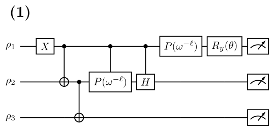
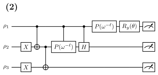
Figure 8: Circuits for implementing a destructive $3$-cycle test. The input state is $\rho_{1}\otimes\rho_{2}\otimes\rho_{3}$. The circuits start with application of a Pauli $X$-gate that depends on the circuit index (k): in the circuit (1), it is applied to the first qubit, while the circuit (2) applies it to the second and third qubits. They are followed by two CNOT gates, controlled phase gate, and controlled Hadamard gate. The circuits are concluded by application of a phase gate and a $Y$-rotation gate on angle $\theta$ on the first qubit, where $\theta=-2\mathrm{arccos}(1/\sqrt{3})$, so that $R_{y}(\theta)=\nicefrac{{1}}{{\sqrt{3}}}(\mathbb{1}+i\sqrt{2}\,Y)$. The phase gate is defined as $P(\omega^{-\ell})=|0\rangle\langle 0|+\omega^{-\ell}|1\rangle\langle 1|$, corresponding to estimation of probabilities $p_{\ell}^{(k)}$ in (32), and $\omega=e^{2\pi i/3}$. Finally, all qubit get locally measured in the computational basis, providing the necessary statistics for Eq. (31).

To the best of our knowledge, a destructive cycle test had not been introduced before. Nonetheless, Ref. [83] had previously observed that $\langle\mathtt{CYC}_{3}\rangle_{\varrho}$ can be written as the average of two measurements, arriving at a conclusion that is similar in spirit to ours.

V Discussion and outlook

In this work, we have generalized the quantum circuits proposed by Chiribella et al. [69] to estimate multivariate traces of quantum states, introducing a measurement-enhanced cycle test. By leveraging prior classical information about observables, our protocol reduces the quantum resources required to estimate Bargmann invariants of order $n$, cutting the number of qubits and Fredkin gates by up to half compared to the standard cycle test. This trade-off—exchanging classical descriptions of $m$ states for reduced quantum hardware demands—makes our protocol particularly suitable for near-term quantum devices, where qubit counts and gate fidelities are limiting factors.

The ability to estimate higher-order invariants with limited quantum resources opens new opportunities for practical applications. For instance, in extended Kirkwood-Dirac (KD) quasiprobability distributions [37, 34, 35, 36] the defining bases are often classically known. Our protocol allows for the efficient estimation of extended KD distributions even when only a small quantum processor is available. As another example, in the context of sequential weak values [59, 84, 85] one estimates high-order multivariate traces of states where two states—namely the pre- and post-selected states—are assumed to be classically known. Yet another example might be that of estimating geometric phases. It is conceivable that one’s goal is to estimate the geometric phase with respect to a closed path of $n=n^{\prime}+m$ points in projective space, where $n^{\prime}$ of these are unknown vector states while $m$ are classically known by the experimenter. Our protocol allows, in such situations, for the estimation of all the relevant Bargmann invariant phases.

The usefulness of enhancing generic Hadamard tests—not only cycle tests—by also measuring subsystems that are usually left unmeasured was also recently investigated in Ref. [86]. Although the authors do not focus on the problem of multivariate trace estimation, their analysis shows that the Hadamard test can be powered by local (or global) classical shadows of the quantum system usually left unmeasured to extract additional useful information.

We have also shown how to estimate third-order invariants of pure states using multiple instances of the destructive swap test. However, we find limited practical relevance for this approach, as the required number of circuit implementations is comparable to performing full state tomography on the two unknown, given qubit states. This represents evidence that variations of the destructive swap test—unlike its non-destructive counterpart, the standard swap test—may not efficiently leverage the trade-off between classical prior information and quantum resources for estimating higher-order invariants. Still, we have described how to implement destructive cycle tests, and presented a quantum circuit implementation for estimating third-order invariants.

Future work could explore experimental implementations on existing hardware (e.g., superconducting or photonic platforms) and extend the protocol for the destructive swap test to mixed states of arbitrary dimension. Another interesting direction concerns protocols exploiting controlled causal order of measurements, for example, in a experimentally implementable setup known as the quantum SWITCH [87, 88], which has found various applications in quantum theory [89, 90, 91, 92, 93, 94, 95, 96, 97, 98, 99, 100, 101, 102, 103, 104, 105]. In this setup, quantities like out-of-time-correlators [106] and incompatibility of quantum observables [55] can be efficiently estimated. These advances would further solidify the role of Bargmann invariants as versatile tools for the certification of quantum resources in a basis-independent way.