On the (Non) Injectivity of Piecewise Linear Janossy Pooling

Abstract

Multiset functions, which are functions that map multisets to vectors, are a fundamental tool in the construction of neural networks for multisets and graphs. To guarantee that the vector representation of the multiset is faithful, it is often desirable to have multiset mappings that are both injective and bi-Lipschitz. Currently, there are several constructions of multiset functions achieving both these guarantees, leading to improved performance in some tasks but often also to higher compute time than standard constructions. Accordingly, it is natural to inquire whether simpler multiset functions achieving the same guarantees are available. In this paper, we make a large step towards giving a negative answer to this question. We consider the family of $k$-ary Janossy pooling, which includes many of the most popular multiset models, and prove that no piecewise linear Janossy pooling function can be injective. On the positive side, we show that when restricted to multisets without multiplicities, even simple deep-sets models suffice for injectivity and bi-Lipschitzness.

1 Introduction

A natural requirement of machine learning models for graphs and point clouds is that they respect the permutation symmetries of the data. A key tool to achieve this is the process of mapping multisets, which are unordered collections of vectors, to a single (ordered) vector which faithfully represents the multiset.

The celebrated deep-sets paper Zaheer et al. (2017) proposed a simple and popular method to map multisets to vectors via elementwise application of a function $f$, followed by sum pooling, namely

$$F(\{\mathbf{x}_{1},\ldots,\mathbf{x}_{n}\})=\sum_{j=1}^{n}f(\mathbf{x}_{j}).$$ (1)

Another popular alternative, which is more computationally demanding but also more expressive (Zweig and Bruna, 2022), sums a function $f(x_{i},x_{j})$ over all pairs of points

$$F(\{\mathbf{x}_{1},\ldots,\mathbf{x}_{n}\})=\sum_{i,j=1}^{n}f(\mathbf{x}_{i},\mathbf{x}_{j})$$ (2)

This type of pairwise summation allows incorporation of relational pooling (Santoro et al., 2017), or attention mechanisms as proposed in the set-transformer paper (Lee et al., 2019).

A natural generalization of both these models is the notion of $k$-ary Janossy pooling, where a function $f$ is applied to all $k$-tuples of the multiset and then summation is applied to all these $k$-tuples. Deep sets model correspond to the case $k=1$ while set transformers correspond to $k=2$. Janossy pooling for general $k$ was successfully used in Murphy et al. (2019).

To ensure the quality of the vector representation of the multiset, a common requirement is that the function $F$ is injective. This requirement enables construction of maximally expressive message passing neural networks (Xu et al., 2018; Morris et al., 2019), and is exploited in a variety of other scenarios where expressivity of graph neural networks is analyzed (Maron et al., 2019; Hordan et al., 2024a; Sverdlov and Dym, 2025; Zhang et al., 2024)

The inejctivity requirement can be satisfied even by deepsets models, providing that the function $f:\mathbb{R}^{d}\to\mathbb{R}^{m}$ in (1) is defined correctly, and the embedding dimension $m$ is large enough. The various aspects of this question are discussed in Wagstaff et al. (2022); Zaheer et al. (2017); Xu et al. (2018); Amir et al. (2023); Tabaghi and Wang (2024); Wang et al. (2024). Most relevant to our discussion are the recent results which show that (1) can be injective when $f$ is a neural network with smooth activations, but can never be injective when $f$ is a Continuous Piecewise Linear (CPwL) function (as is the case when $f$ is a neural network with ReLU activations).

While these theoretical results seem to indicate an advantage of smooth functions $f$ over CPwL ones, empirical evidence indicates that the separation between multisets via smooth activations can be very weak Bravo et al. (2024); Hordan et al. (2024b), and that empirically the separation obtained even by non-injective CPwL deep sets model is often preferable. Thus, recent papers have argued that a more refined notion of separation is necessary, via the notion of bi-Lipschitz stability Davidson and Dym (2025); Amir and Dym (2025); Balan et al. (2022). In this notion, multisets are required not only to be mapped to distinct vectors, but we also require that the distance between the vector representations resembles the natural Wasserstien distance between the multisets.

In the lens of bi-Lipschitz stablility, the ranking of CPwL and smooth multiset functions are reversed. In fact, Amir et al. (2023) and Cahill et al. (2024) showed that smooth multiset functions can never be bi-Lipshitz. In contrast, while CPwL deepsets functions are not injective (or bi-Lipschitz), several recent papers have suggested new CPwL multiset-to-vector mappings based on sorting (Balan et al., 2022; Dym and Gortler, 2024; Balan and Tsoukanis, 2023), Fourier sampling of the quantile function Amir and Dym (2025), or max filters Cahill et al. (2022), and showed that they are both injective and bi-Lipschitz. In fact, Sverdlov et al. (2024) showed that CPwL multiset functions which are injective are automatically also bi-Lipschitz.

Experimentally, it was shown that these CPwL bi-Lipschitz multiset mappings have significant advantages over standard methods, for tasks like learning Wasserstein distances or learning in a low parameter regime (Amir and Dym, 2025) and for graph learning tasks Davidson and Dym (2025) including reduction of oversquashing Sverdlov et al. (2024). On the other hand, these methods are typically more time consuming than standard methods, and at least at the time this paper is written they are not as prevalent as deepsets and set transformers.

The goal of this paper is to address the following question

Main Question: Is it possible to construct CPwL injective (and bi-Lipschitz) functions via $k$-ary pooling?

Currenlty, we have a negative answer to this question only in the special case where $k=1$ (deepsets), but for $k\geq 2$ (e.g. set transformers) the answer is unknwon. A positive answer to this question would potentially lead to new bi-Lipschitz models which are closer to established models like set transformers, and potentially would have better performance. A negative answer would indicate that bi-Lipschitz models do require different types of multiset functions, such as the sort based functions currenly suggested in the literature.

Main Results

Our theoretical analysis reveals two main results. The first result is that in full generality, the answer to our main question is negative: $k$-ary Janossy pooling is not injective, except in the unrealistic scenario where $k$ is equal to the full cardinality of the multiset. This result strengthens the argument for using sorting based bi-Lipchitz mappings as in (Davidson and Dym, 2025; Amir and Dym, 2025; Sverdlov et al., 2024).

Our second result shows that the obstruction to injectivity is only the existence of multisets with repeated points: on a compact domain $D$ of multisets where all multisets have distinct points, even the $1$-ary CPwL Janossy pooling (deepsets) can be injective and bi-Lipschitz. The computational burden of this construction strongly depends on a constant $R(D)$ which measures how close multisets in $D$ are to have repeated points. This result suggests that the advantages provided by sort-based methods may only be relevant in datasets where (near) point multiplicity occurs (e.g. point cloud samples of surfaces where points are very close together), and not in datasets where points are typically fairly far away, such as multisets which describe small molecules.

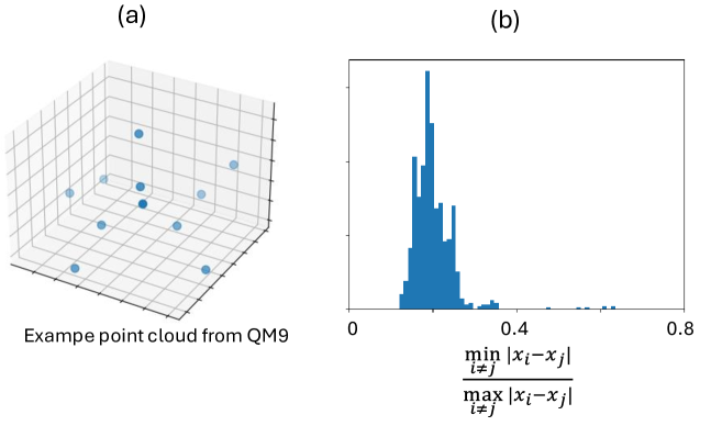
Figure 1: This figure illustrates that the assumption that multisets do not have (near)-repeated points is realistic for small molecule datasets. In (a) we show an example multiset from the QM9 (Ruddigkeit et al., 2012; Ramakrishnan et al., 2014) small molecule dataset. This example shows visually that different set elements are not very close together. In (b) we see the statistics of the minimal distance within each multiset (normalized by the maximal distance), over 1,000 represetative samples from QM9. In all these instances, the minimal distance was never lower than $0.1$.

Paper Structure

In Section 2 we will lay out the formal definitions needed to fully define our problem. In Section 3 we state and prove the non-injectivity of CPwL Janossy pooling for general domains, and in Section 4 we state and prove the injectivity results for domains with non-repeated elements. Conclusions, Limitations and future work are discussed in Section 5.

2 Problem Statement

We begin by formally stating the notions necessary to define our problem. For arbitrary sets $C,Y$, we say that a function $F:C^{n}\to Y$ is permutation invariant if $F(\mathbf{w}_{1},\ldots,\mathbf{w}_{n})=F(\mathbf{w}_{\pi(1)},\ldots,\mathbf{w}_{\pi(n)})$ for every permutation $\pi$ of the coordinates of $\mathbf{w}\in C^{n}$.

The notion of permutation invariant functions is closely linked to the notion of functions on multisets. A multiset $\{\mathbf{w}_{1},\ldots,\mathbf{w}_{n}\}$ is a collection of elements which is unordered (like sets), but where repetitions are allowed (unlike sets). We denote the space of multisets by $\mathcal{M}_{n}(C)$.

If $F$ is permutation invariant, we can identify it with a function on multisets in $\mathcal{M}_{n}(C)$ via

$$F\left(\{\mathbf{w}_{1},\ldots,\mathbf{w}_{n}\}\right)=F(\mathbf{w}_{1},\ldots,\mathbf{w}_{n})$$

Since $F$ is permutation invariant, this expression is well defined and does not depend on the ordering. Conversely, any multiset function $F$ on $\mathcal{M}_{n}(C)$ can be used to define a permutation invariant function on $C^{n}$. Due to this identification, we will use the term ’multiset function’ and ’permutation invariant function’ alternatingly, according to convenience.

In this paper, our main focus is on permutation invariant functions defined by $k$-ary Janossy pooling. Namely, for some natural numbers $k\leq n$, and a function $f:C^{k}\to Y$, we define a permutation invariant function $F:C^{n}\to Y$ via

$$F(\mathbf{x}_{1},\dots,\mathbf{x}_{n})=\frac{1}{(n-k)!}\sum_{\pi\in S_{n}}f\left(\mathbf{x}_{\pi(1)},\dots,\mathbf{x}_{\pi(k)}\right)$$ (3)

As mentioned above, special cases of Janossy pooling include the deep sets model in (1), which corresponds to the case $k=1$, and set transformer models which correspond to the case $k=2$ (2).

As discussed in the introduction, we will focus on the case where the function $f$ used to define the Janossy pooling is Continuous Piecewise Linear (CPwL). To define this, we recall that a (closed, convex) polytope $P$ is a subset of $\mathbb{R}^{d}$ defined by a finite number of weak inequalities

$$P=\{\mathbf{x}\in\mathbb{R}^{d}|\mathbf{a}_{j}\cdot\mathbf{x}+b_{j}\geq 0,\forall j=1,\ldots,J\}$$

A partition of $\mathbb{R}^{d}$ is a finite collection of polytopes with non-empty interior, whose union covers $\mathbb{R}^{d}$ and whose interiors do not intersect. A CPwL function $f:\mathbb{R}^{d}\to\mathbb{R}^{m}$ is a continuous function satisfying that, for some partition $\mathcal{P}=\{P_{1},\ldots,P_{k}\}$, the restriction of $f$ to each polytope $P_{j}$ in the partition is an affine function. The polytopes $P_{j}$ are called linear regions of $f$. Neural networks defined by piecewise linear activations like ReLU or leaky ReLU are important examples of CPwL functions.

Finally, a multiset function $F:\mathcal{M}_{n}(C)\to Y$ is injective if it is injective in the standard sense: for all distinct multisets $W,W^{\prime}\in\mathcal{M}_{n}(C)$ we have $F(W)\neq F(W^{\prime})$. As discussed in the introduction, the question we discuss in this paper is the injectivity of $F$ induced from Janossy pooling of a CPwL function $f$.

3 Non-injectivity of Janossy Pooling for general domains

Now we can state our main theorem:

Theorem 3.1.

[Non-Injectivity of $k$-ary Janossy Pooling of CPwL functions] Let $C$ be a subset of $\mathbb{R}^{d}$ that contains a line segment (usually this will be $[0,1]^{d}$ or $\mathbb{R}^{d}$ itself). Let $f:(\mathbb{R}^{d})^{k}\rightarrow\mathbb{R}^{m}$ be a continuous piecewise linear (CPwL) function. Let $n>k$, and let $F:(\mathbb{R}^{d})^{n}\rightarrow\mathbb{R}^{m}$ be the $k$-ary Janossy pooling of $f$. Then $F$ is not injective on $\mathcal{M}_{n}(C)$.

To provide intuition for the theorem, we recall the simple proof for the simple case $k=1,d=1$, provided in Amir et al. (2023). In this case, we find a pair of distinct points $x,y$ which are in the same linear region of $f$. In this case, the average of $x$ and $y$ is also in the same linear region, and we can use this to obtain a contradiction to injectivity

$$F(x,y)=f(x)+f(y)=f(\frac{x+y}{2})+f(\frac{x+y}{2})=F(\frac{x+y}{2},\frac{x+y}{2}).$$

The proof of the case $k=1,d=1$ relies on the trivial observation that we can always find a pair of numbers $(x,y)\in\mathbb{R}^{2}$ (or more generally in $\mathbb{R}^{n}$) whose elements are distinct, but come from the same partition which the CPwL function $f:\mathbb{R}\to\mathbb{R}^{m}$ is subordinate to. To generalize this result to $k$-ary pooling, we will need to show a similar but much stronger property: for any polytope partition of $\mathbb{R}^{k}$, one can only find a vector in $\mathbb{R}^{n}$ of distinct monotonely decreasing elements, such that all $k$-ary montonely ordered subvectors belong to a single polytope from the partition:

Theorem 3.2.

For every polytope partion $\mathcal{P}$ of $\mathbb{R}^{k}$, there exists a polytope $P_{0}\in\mathcal{P}$ and a point $\mathbf{w}=(w_{1},\dots,w_{n})\in(0,1)^{n}$ such that $w_{1}>\dots>w_{n}$ and, for any ascending $k$-tuple of indices $i_{1}<\dots<i_{k}$ in $[n]$, the point $(w_{i_{1}},\dots,w_{i_{k}})$ is in $\mathrm{int}(P_{0})$.

A visualization of the property described in the theorem is provided in Figure 2 for the special case $k=2,n=3$.

[capbesideposition=right,top,capbesidewidth=5cm]figure[]

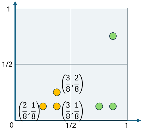
Figure 2: Visualization of the property from Theorem 3.2 for a partition of $[0,1]^{2}$ into four squares. The point $\mathbf{w}=(3/8,2/8,1/8)$ fulfills the conditions of the proposition, as all three $2$ dimensional ordered subvectors are in the same square (see orange dots). The vector $(7/8,6/8,1/8)$ does not fulfill the condition (see green dots)

To the best of our knowledge, Theorem 3.2 has not previously been known. The proof of this result is technical and non-trivial and it is given in the Appendix.

We now explain how this proposition can be used to prove Theorem 3.1.

Proof of Theorem 3.1.

For the sake of simplicity we first prove the theorem in the case $d=1$. We will later easily generalize this result to the general case $d>1$. We assume WLOG that $C=[0,1]$.

Let $f:\mathbb{R}^{k}\rightarrow\mathbb{R}^{m}$ be a CPwL function. Let $F:\mathbb{R}^{n}\rightarrow\mathbb{R}^{m}$ be its $k$-ary Janossy pooling as in (3). Our goal is to prove that $F$ is not injective on multisets $\mathcal{M}_{n}([0,1])$.

The first step is to show that $F$ can be defined alternatively by applying Janossy pooling to the permutation invariant function $\hat{f}:\mathbb{R}^{k}\rightarrow\mathbb{R}^{m}$ defined by

$$\hat{f}(x_{1},\dots,x_{k})=\sum_{\pi\in S_{k}}f\left(x_{\pi(1)},\dots,x_{\pi(k)}\right)$$

Note that $\hat{f}$ is a permutation-invariant function and that we can equivalently write

$$F(x_{1},\dots,x_{n})=\sum_{1\leq i_{1}<\dots<i_{k}\leq n}\hat{f}\left(x_{i_{1}},\dots,x_{i_{k}}\right)$$

Summing over all $\binom{n}{k}$ subsets of $[n]$ of size $k$.

Note that $\hat{f}$ is the sum of finitely many CPwL functions; therefore, it is itself a CPwL function. Let $\mathcal{P}$ be a finite polytope covering of $[0,1]^{k}$ such that for all polytopes $P\in\mathcal{P}$, $\hat{f}\big{|}_{P}$ is an affine function. Let $P_{0}$ be as promised from Theorem 3.2, and let $A\in\mathbb{R}^{m\times k},\mathbf{b}\in\mathbb{R}^{m}$ such that $\hat{f}\big{|}_{P_{0}}(\mathbf{z})=A\mathbf{z}+\mathbf{b}$. The properties of the point $\mathbf{w}$ in the theorem are preserved under small perturbations. Namely, for some $r>0$, we have that for all vectors $\boldsymbol{\delta}\in\mathbb{R}^{n}$ with norm bounded by $r$, we will have both $w_{1}+\delta_{1}>w_{2}+\delta_{2}>\ldots>w_{n}+\delta_{n}$, and that all $k$ vectors obtained from $\mathbf{w}+\boldsymbol{\delta}$ by choosing $k$ different ascending indices will be in the same polytope $P_{0}$. It follows that for all such $\boldsymbol{\delta}$

$$F(\mathbf{w}+\boldsymbol{\delta}) =\sum_{1\leq i_{1}<\dots<i_{k}\leq n}\hat{f}\left(w_{i_{1}}+\delta_{i_{1}},\dots,w_{i_{k}}+\delta_{i_{k}}\right)$$

$$=\binom{n}{k}\mathbf{b}+\sum_{1\leq i_{1}<\dots<i_{k}\leq n}A\left(w_{i_{1}}+\delta_{i_{1}},\dots,w_{i_{k}}+\delta_{i_{k}}\right)^{\top}$$

$$=\binom{n}{k}\mathbf{b}+A\left(\sum_{1\leq i_{1}<\dots<i_{k}\leq n}\left(w_{i_{1}}+\delta_{i_{1}},\dots,w_{i_{k}}+\delta_{i_{k}}\right)^{\top}\right)$$

To contradict injectivity we will want to obtain $F(\mathbf{w})=F(\mathbf{w}+\boldsymbol{\delta})$, which will hold if

$$\sum_{1\leq i_{1}<\dots<i_{k}\leq n}\left(\delta_{i_{1}},\dots,\delta_{i_{k}}\right)=\left(0,\dots,0\right)$$

Indeed, these are $k$ linear homogenous equations in $n>k$ variables, and they have a non zero solution $\boldsymbol{\delta}$. We can scale this $\boldsymbol{\delta}$ by a sufficient small number to guarantee that $\|\boldsymbol{\delta}\|<r$. We then have that $F(\mathbf{w})=F(\mathbf{w}+\boldsymbol{\delta})$, that $\mathbf{w}+\boldsymbol{\delta}\neq\mathbf{w}$, and moreover, since both $\mathbf{w}$ and $\mathbf{w}+\boldsymbol{\delta}$ are sorted from small to large, that $\mathbf{w}$ is not a permutation of $\mathbf{w}+\boldsymbol{\delta}$. Thus $F$ is not injective, and we proved the theorem in the case where $d=1$.

When $d>1$. We now prove the general case $d>1$ by a reduction to the case $d=1$. Let us assume by contradiction that $C\subseteq\mathbb{R}^{d}$ contains the line segment between some (non-identical) points $\boldsymbol{\alpha}$ and $\boldsymbol{\beta}$, that $f$ is some CPwL function and that the function $F$ obtained by $k$-ary Janossy pooling on $f$ is injective.

Let $g:[0,1]\to C$ be the affine function $g(t)=(1-t)\boldsymbol{\alpha}+t\boldsymbol{\beta}$. For any natural $s$, we can extend $g$ to a mapping $g^{(s)}:[0,1]^{s}\to(\mathbb{R}^{d})^{s}$ by applying $g$ to each coordinate, i.e., for $\mathbf{t}=(t_{1},\dots,t_{k})\in[0,1]^{s}$, $g^{(s)}(\mathbf{t})=(g(t_{1}),\dots,g(t_{s}))$. The function $g^{(s)}$ is affine and injective. Accordingly, the function $F\circ g^{(n)}:C^{n}\to\mathbb{R}^{m}$ is injective, and we note that it is the Janossy pooling of $f\circ g^{(k)}$ which is a CPwL function as the composition of a CPwL function and an affine function. This leads to a contradiction to our proof for the case $d=1$. ∎

3.1 Janossy pooling when $k=n$

In the degenerate case where we use $n$-ary pooling for multisets of cardinality $n$, an expensive averaging over all permutations is necessary. In this case we can choose the initial $f$ we use to be a CPwL multiset injective function, such as the sorting based functions constructed in Balan et al. (2022) and mentioned earlier. Since the initial $f$ is already permutation invariant, and $n=k$, we would obtain $F(\mathbf{x}_{1},\ldots,\mathbf{x}_{n})=f(\mathbf{x}_{1},\ldots,\mathbf{x}_{n})$ in this case, and so Janossy pooling of CPwL functions can be injective in this degenerate case.

4 Injectivity under restricted domains

We now discuss our second main result. In contrast to the non-injectivity result presented in the previous section for general multiset domains of the form $\mathcal{M}_{n}(C)$, we now show that by restricting the domain to a compact $D\subset\mathcal{M}_{n}(C)$ where each multiset has $n$ distinct elements, injective $1$-ary Janossy pooling is possible. To state this theorem formally, we define the natural Wasserstein metric on the space of multiset, and then the notion of a compact set in multiset-space:

Definition 4.1.

Given two multisets $A,B\in\mathcal{M}_{n}(\mathbb{R}^{d})$, the Wasserstein metric $d_{W}(A,B)$ is defined as

$$d_{W}(A,B)=\min_{\sigma\in S_{n}}\sum_{i=1}^{n}\|\mathbf{a}_{i}-\mathbf{b}_{\sigma(i)}\|$$

where $A=\{\mathbf{a}_{1},\mathbf{a}_{2},\dots,\mathbf{a}_{n}\}$, $B=\{\mathbf{b}_{1},\mathbf{b}_{2},\dots,\mathbf{b}_{n}\}$, $S_{n}$ is the set of all permutations of $[n]$, and $\|\cdot\|$ denotes the $\ell_{\infty}$ norm. Note that the expression above is permutation invariant, and therefore well-defined independently of the order of the elements of $A,B$.

Definition 4.2.

Let $C\subset\mathbb{R}^{d}$. We say that $D\subset\mathcal{M}_{n}(C)$ is compact if every sequence of multisets $\{A_{j}\}_{j=1}^{\infty}$ in $D$ has a subsequence that converges to a multiset in $D$ with respect to the Wasserstein metric $d_{W}$. This is the standard definition of compactness in a metric space.

We can now state our second main result: in the absence of multisets with repeated elements, even $1$-ary pooling is injective:

Theorem 4.3.

Let $D\subset\mathcal{M}_{n}(C)$ be a compact set of multisets where each multiset has $n$ distinct elements. Then there exists some $m=m(D)$ and a continuous piecewise linear function $f:\mathbb{R}^{d}\rightarrow\mathbb{R}^{m}$ such that its $1$-ary Janossy pooling $F(A)=\sum_{\mathbf{a}\in A}f(\mathbf{a})$ is injective on $D$, and bi-Lipschitz with respect to the Wasserstein distance.

We will prove this theorem by construction. We begin with some preliminaries: we first introduce the minimal separation function $r:D\rightarrow\mathbb{R}_{\geq 0}$ via

$$r(A)=\min_{\begin{subarray}{c}\mathbf{a}_{i},\mathbf{a}_{j}\in A\\ i\neq j\end{subarray}}\|\mathbf{a}_{i}-\mathbf{a}_{j}\|$$

for any multiset $A=\{\mathbf{a}_{1},\mathbf{a}_{2},...,\mathbf{a}_{n}\}\in D$, where $\|\cdot\|$ denotes the $\ell_{\infty}$ norm. We note that by our theorem’s assumptions, $r(A)>0$ for all $A\in D$. We next define $R(D)$ to be the minimal separation obtained on all of $D$, namely

$$R(D)=\inf_{A\in D}r(A)=\inf_{A\in D}\min_{\begin{subarray}{c}\mathbf{a}_{i},\mathbf{a}_{j}\in A\\ i\neq j\end{subarray}}\|\mathbf{a}_{i}-\mathbf{a}_{j}\|.$$

We next show that, due to the compactness of $D$, the infimum in the definition of $R(D)$ is obtained and $R(D)$ is always strictly positive.

Proposition 4.4.

If $D\subset\mathcal{M}_{n}(C)$ is a compact set of multisets, where each multiset $A\in D$ consists of $n$ distinct elements, then its minimum separation $R(D)$ is positive.

Proof.

Assume, for the sake of contradiction, that $R(D)=0$. By the definition of the infimum, this implies that there exists a sequence of multisets $\{A_{j}\}_{j=1}^{\infty}$ in $D$ such that $r(A_{j})\rightarrow 0$ as $j\rightarrow\infty$. Each $A_{j}=\{\mathbf{a}_{1}^{(j)},\dots,\mathbf{a}_{n}^{(j)}\}$ consists of $n$ distinct points.

Since $D$ is compact, the sequence $\{A_{j}\}_{j=1}^{\infty}$ has a subsequence $\{A_{j_{l}}\}_{l=1}^{\infty}$ that converges to a multiset $A^{*}\in D$ with respect to the Wasserstein metric $d_{W}$. Let $A^{*}=\{\mathbf{a}_{1}^{*},\dots,\mathbf{a}_{n}^{*}\}$. By definition of $D$, we have $r(A^{*})>0$.

Let $\epsilon=\frac{r(A^{*})}{2}$. From the convergence of $r(A_{j_{l}})$ and $A_{j_{l}}$, there exists an $l$ such that $r(A_{j_{l}})<\epsilon$ and $d_{w}(A_{j_{l}},A^{*})<\epsilon$. For this $l$, we deduce there are at least two distinct points, WLOG $a_{1}^{(j_{l})},a_{2}^{(j_{l})}\in A_{j_{l}}$, such that $\|a_{1}^{(j_{l})}-a_{2}^{(j_{l})}\|<\epsilon$. Next, let $\sigma\in S_{n}$ be the permutation such that the minimum in the definition of the Wasserstein distance between $A^{*},A_{j_{l}}$ is attained. Then, applying the triangle inequality twice, we get:

$$\frac{r(A^{*})}{2}=\epsilon >d_{w}(A_{j_{l}},A^{*})$$

$$=\sum_{i=1}^{n}\|\mathbf{a}^{(j_{l})}_{i}-\mathbf{a}^{*}_{\sigma(i)}\|$$

$$\geq\|\mathbf{a}^{(j_{l})}_{1}-\mathbf{a}^{*}_{\sigma(1)}\|+\|\mathbf{a}^{(j_{l})}_{2}-\mathbf{a}^{*}_{\sigma(2)}\|$$

$$\geq\|\mathbf{a}^{*}_{\sigma(1)}-\mathbf{a}^{*}_{\sigma(2)}+\mathbf{a}^{(j_{l})}_{2}-\mathbf{a}^{(j_{l})}_{1}\|$$

$$\geq\|\mathbf{a}^{*}_{\sigma(1)}-\mathbf{a}^{*}_{\sigma(2)}\|-\|\mathbf{a}^{(j_{l})}_{1}-\mathbf{a}^{(j_{l})}_{2}\|$$

$$\geq r(A^{*})-\epsilon=\frac{r(A^{*})}{2}$$

This is a contradiction. We conclude that $R(D)>0$. ∎

We now provide the construction of the function $f$. Tessellate $\mathbb{R}^{d}$ with a grid of non-overlapping, adjacent $d$-dimensional hypercubes $Q_{k}$, each with side length $s=\frac{R(D)}{2}$.

We define a $\delta$-margin around each hypercube $Q_{k}$ using the $\ell_{\infty}$ distance. For any point $\mathbf{x}$, its $\ell_{\infty}$ distance to the hypercube $Q_{k}$ is given by $d_{\infty}(\mathbf{x},Q_{k})=\min_{\mathbf{y}\in Q_{k}}||\mathbf{x}-\mathbf{y}||_{\infty}$. The $\delta$-margin of $Q_{k}$ is then the set of points $\{\mathbf{x}\in\mathbb{R}^{d}\setminus Q_{k}\mid d_{\infty}(\mathbf{x},Q_{k})<\delta\}$.

Let $\delta$ be a margin width chosen such that $0<\delta<\frac{R(D)}{4}$. This ensures that the equation $(s+2\delta)<R(D)$ is satisfied. This implies that if a hypercube $Q_{k}$ together with its $\delta$-margin contains a point $\mathbf{a}\in A$ (for $A\in D$), it cannot contain any other point $\mathbf{a}^{\prime}\in A\setminus\{\mathbf{a}\}$. In particular, $Q_{k}$ itself, can contain at most one point from $A$.

Let $\mathcal{I}$ be the finite set of indices of hypercubes $Q_{k}$ that intersect $C^{\prime}=\bigcup_{A\in D}A\subseteq C$. Since $D$ is compact, $C^{\prime}$ is bounded, ensuring $\mathcal{I}$ is finite.

For each hypercube $Q\in\{Q_{k}\}_{k\in\mathcal{I}}$, we define a local $(d+1)$-dimensional feature vector $f_{Q}(\mathbf{x})$, consisting of two components:

Indicator Component $f_{Q,\text{ind}}(\mathbf{x})\in[0,1]$: $f_{Q,\text{ind}}(\mathbf{x})=1$ if $\mathbf{x}\in Q$, and $f_{Q,\text{ind}}(\mathbf{x})=\max(0,1-d_{\infty}(\mathbf{x},Q)/\delta)$ elsewhere. This ensures $f_{Q,\text{ind}}(\mathbf{x})=1\iff\mathbf{x}\in Q$, and that the support of $f_{Q,\text{ind}}$ is precisely $Q$ together with is $\delta$-margin. Note that this component is CPwL.

Relative Coordinate Component ($\mathbf{f}_{Q,\text{coords}}(\mathbf{x})\in\mathbb{R}^{d}$): This is a CPwL function defined by the following properties:

• If $\mathbf{x}\in Q$, then $\mathbf{f}_{Q,\text{coords}}(\mathbf{x})=\mathbf{x}$.

• If $\mathbf{x}$ is located outside $Q$ and its $\delta$-margin (i.e., $d_{\infty}(\mathbf{x},Q)\geq\delta$), then $\mathbf{f}_{Q,\text{coords}}(\mathbf{x})=\mathbf{0}$.

• In the $\delta$-margin (i.e., for $\mathbf{x}$ such that $0<d_{\infty}(\mathbf{x},Q)<\delta$), $\mathbf{f}_{Q,\text{coords}}(\mathbf{x})$ interpolates continuously and piecewise linearly between the values at $\partial Q$, and $\mathbf{0}$ at the outer boundary of the margin.

We shall now demonstrate how a function satisfying the third condition can be constructed. By Goodman and Pach (1988), the $\delta$-margin can be triangulated without introducing new vertices such that each simplex of the triangulation contains vertices belonging to both $Q$ and the outer border of the margin.

It is well known that given a simplex in $\mathbb{R}^{d}$ defined by $d+1$ affinely independent points $p_{0},\ldots,p_{d}$, and corresponding values $y_{0},\ldots,y_{d}$, there exists a unique affine function $h$ such that $h(x_{i})=y_{i}$ for all $i$.

Applying this to our triangulated $\delta$-margin, we define $f$ piecewise over each simplex by assigning the known values of $f$ at its vertices—values from $Q$ and zeros from the outer border. The unique affine interpolation over each simplex ensures that $f$ transitions continuously between the identity on $Q$ and zero on the outer region, satisfying the desired conditions.

Constructions of this sort are standard in numerical analysis and finite element methods. For instance, in the context of simplicial finite elements, the $\mathbb{P}_{1}$ interpolant of a function $v$ is the unique piecewise affine function that coincides with $v$ at the mesh vertices (see, e.g., (Brenner and Scott, 2008, 3.3)).

The function $f_{Q}(\mathbf{x})=(f_{Q,\text{ind}}(\mathbf{x}),\mathbf{f}_{Q,\text{coords}}(\mathbf{x}))$ is therefore CPwL.

The overall function $f:\mathbb{R}^{d}\rightarrow\mathbb{R}^{m}$ is the concatenation $f(\mathbf{x})=(\dots,f_{Q_{k}}(\mathbf{x}),\dots)_{k\in\mathcal{I}}$. The output dimension is $m=|\mathcal{I}|\cdot(d+1)$.

Now that we have defined the CPwL function $f$ we will use for the proof, we formally conclude the proof:

Proof of Theorem 4.3.

Let $A\in D$ be a multiset $\{\mathbf{a}_{1},\dots,\mathbf{a}_{n}\}$. The $1$-ary Janossy pooling is $F(A)=\sum_{j=1}^{n}f(\mathbf{a}_{j})$. We show $A$ can be uniquely recovered from $F(A)$. Let $F_{Q_{k},\text{ind}}$ and $\mathbf{F}_{Q_{k},\text{coords}}$ be the components of $F(A)$ corresponding to $Q_{k}$. We first prove two simple lemmas

Lemma 4.5.

$F_{Q_{k},\text{ind}}(A)=1$ if and only if there exists a unique $\mathbf{a}\in A$ such that $\mathbf{a}\in Q_{k}$.

Proof.

($\Rightarrow$) Suppose $F_{Q_{k},\text{ind}}(A)=1$. Assume for the sake of contradiction that there is no $\mathbf{a}\in A$ such that $\mathbf{a}\in Q_{k}$. The support of $f_{Q,\text{ind}}$ is $Q_{k}$ together with its $\delta$-margin. For all $\mathbf{a}$ in this margin, $0<f_{Q,\text{ind}}(\mathbf{a})<1$. However,

$$F_{Q_{k},\text{ind}}(A)=\sum_{j=1}^{n}f_{Q_{k},\text{ind}}(\mathbf{a}_{j})=1$$

This implies that at least two elements of $A$ lie in the $\delta$-margin of $Q_{k}$, which is a contradiction to the separation condition that $\delta$ was constructed to satisfy.

($\Leftarrow$) Suppose there exists $\mathbf{a}\in A$ such that $\mathbf{a}\in Q_{k}$. By construction of $s$ and $\delta$, no other element of $A$ lies in the support of $f_{Q,\text{ind}}$. Therefore,

$$F_{Q_{k},\text{ind}}(A)=f_{Q_{k},\text{ind}}(\mathbf{a})=1$$

∎

Lemma 4.6.

If $\mathbf{a}\in A$ lies in a hypercube $Q_{k}$, then

$$\mathbf{F}_{Q_{k},\text{coords}}(A)=\mathbf{f}_{Q_{k},\text{coords}}(\mathbf{a})=\mathbf{a}$$

Proof.

The proof is similar to the direction ($\Leftarrow$) in the proof of 4.5. ∎

We now prove that $A$ can be recovered uniquely from $F(A)$. We do this using the following procedure. We go over all hypercubes $Q_{k}$. We then check whether $F_{Q_{k},\text{ind}}(A)=1$. By Lemma4.5 we know that this is the case if and only if $A$ contained an element in $Q_{k}$, and in this case the element is unique. We can now recover this element from $F_{Q_{k},\text{coords}}$ using Lemma 4.6. We have thus uniquely recovered all elements of $A$. We note that if $A$ contains elements which are in the intersection of several hypercubes, this reconstruction procedure will give us the same elements of $A$ from several different hypercubes. This does not cause any issues since we know that $A$ does not contain multiplicities.

Finally, to prove the bi-Lipschitzness of the construction: we note that the set $D$ could be covered by a finite union of polytopes (e.g. hypercubes) so that the union of all these hypercubes $\hat{D}$ contains $D$ but still does not contain multisets with repeated elments. As we now proved, we can construct a CPwL function $f$ so that the resulting $F$ obtained from 1-ary Janossy pooling will be injective on $\hat{D}$. Since $F$ and the 1-Wasserstein distance are both CPwL functions which attain the same zeros on $\hat{D}\times\hat{D}$, and $\hat{D}\times\hat{D}$ can be written a a finite union of compact polytopes, We can apply (Sverdlov et al., 2024, Lemma 3.4) to show that $F$ is bi-Lipschitz on each polytope separately, and therefore also on the union which gives us $\hat{D}\times\hat{D}$. ∎

4.1 Dependence on separation

We note that the dimension $m$ which $F,f$ map to in the construction, depends strongly on the separation $R(D)$ and the dimension $d$. If we add the assumption that all elements of multisets $A$ are in the unit cube $[0,1]^{d}$, then a tesselation of side length $\sim R(D)$ would require an embedding dimension of $m\sim(1/R(D))^{d}$. This suggests that when $D$ contains elements which are ’almost identical’, so that $R(D)$ is small, then 1-ary pooling may not really be enough to get a good embedding with an affordable function $f$.

As shortly discussed in the introduction, one possible example where the separation $R(D)$ is reasonably large is small molecules. To examine this, we randomly chose 1000 molecules from the QM9 Ruddigkeit et al. (2012); Ramakrishnan et al. (2014) small molecule datasets. Each molecule is represented as a multiset of vectors residing in $\mathbb{R}^{3}$. For each of these multisets, we computed the minimum distance between multiset elements, and normalized it by the maximal distance between elements. A histogram of the results is shown in Figure1(b). We see that in all instances the ratio was not larger than $1/10$, so we can estimate that a ratio of $R(D)\approx 1/10$ could be reasonable for this type of problem.

5 Conclusion, limitations and future Work

In this paper we showed two main results (a) continuous piecewise linear Janossy pooling is not injective, when considering general domain, and (b) on compact domains with non-repeated points, even $1$-ary continuous piecewise linear Janossy pooling can be injective. These results suggest that deepsets models may be sufficient for tasks where multisets do not have multiplicities (so that they are sets), and the margin between closest points is significant. At the same time, when this margin is small it strengthens the case for using injective and bi-Lipschitz CPwL models such as Davidson and Dym (2025); Amir and Dym (2025), since we show that alternative natural methods cannot attain similar theoretical guarantees.

Building upon our positive result for 1-ary CPwL Janossy pooling on domains of sets (i.e., multisets with point multiplicities of at most one), a natural direction for future work is to explore the capacity of higher-order pooling. We conjecture that for a given integer $k\geq 1$, $k$-ary CPwL Janossy pooling can be injective on compact domains of multisets where the multiplicity of any individual element is at most $k$.

A limitation of this work is that we only analyze the injectivity of CPwL Janossy pooling. Our focus on these functions stems from the fact that CPwL injectivity implies bi-Lipschitzness, while smooth multiset functions, which can be injective via Janossy pooling, cannot be bi-Lipschitz Amir et al. (2023); Cahill et al. (2024). However, there are many functions which are neither CPwL nor smooth. An interesting avenue for future work is investigating whether such functions can be used to construct injective and bi-Lipschitz multiset functions via $k$-ary pooling, and whether these can lead to multiset models with good empirical performance. This question is most interesting for $k=2$ as $2$-ary Janossy pooling has reasonable complexity, and as for $k=1$ such a function can only exist if it is not differentiable at any point Amir et al. (2023).

Acknowledgements N.D. was supported by ISF grant 272/23.

Appendix A Technical Appendix

A.1 Proof of Theorem 3.2

We first establish the following supporting result:

Let $\mathbf{v}\in[0,1]^{k}$. We define $\mathrm{POLY}(\mathbf{v})=\{P\in\mathcal{P}\mid\mathbf{v}\in P\}$ to be the set of polytopes in the covering $\mathcal{P}$ that contain the point $\mathbf{v}$.

Lemma A.1.

Let $\mathbf{v}\in\mathbb{R}^{k}$. Let $\mathcal{P}$ be a finite polytope covering of $\mathbb{R}^{k}$. There exists $\epsilon>0$ such that the $\epsilon$-ball around $\mathbf{v}$ w.r.t. the $\ell_{1}$ metric, denoted by $B_{\ell_{1}}(\mathbf{v},\epsilon)=\{\mathbf{x}\in[0,1]^{k}:\|\mathbf{x}-\mathbf{v}\|_{1}<\epsilon\}$, does not intersect any polytope that does not contain $\mathbf{v}$:

$$B_{\ell_{1}}(\mathbf{v},\epsilon)\cap\bigcup(\mathcal{P}\setminus\mathrm{POLY}(\mathbf{v}))=\emptyset$$

Proof of Lemma A.1.

Let $P\in\mathcal{P}\setminus POLY(\mathbf{v})$. Since $P$ is closed,

$$\mathrm{dist}(\mathbf{v},P)=\inf_{\mathbf{x}\in P}\left\|\mathbf{x}-\mathbf{v}\right\|>0$$

Let

$$\epsilon=\frac{1}{2}\min_{P\in\mathcal{P}\setminus\mathrm{POLY}(\mathbf{v})}\left(\mathrm{dist}(\mathbf{v},P)\right)$$

Since $\mathcal{P}$ is finite, $\epsilon$ is well defined and positive. For this choice of $\epsilon$, we have

$$B_{\ell_{1}}(\mathbf{v},\epsilon)\cap\bigcup(\mathcal{P}\setminus\mathrm{POLY}(\mathbf{v}))=\emptyset$$

∎

Proof of Theorem 3.2.

Fix some $x\in(0,1)$ and let $\mathbf{v}_{0}=(x,\dots,x)\in(0,1)^{k}$.

Using Lemma A.1, let $\epsilon_{1}>0$ such that $B_{\ell_{1}}(\mathbf{v}_{0},\epsilon_{1})\subset\bigcup\mathrm{POLY}(\mathbf{v}_{0})$ and $B_{\ell_{1}}(\mathbf{v}_{0},\epsilon_{1})\subset(0,1)^{k}$.

Let $\mathbf{v}_{1}=\mathbf{v}_{0}+\frac{\epsilon_{1}}{2}\mathbf{e}_{1}=(x+\frac{\epsilon_{1}}{2},x,\dots,x)$.

We continue this construction by an inductive process. For all $1<i\leq k$:

Let $\epsilon_{i}>0$ such that $B_{\ell_{1}}(\mathbf{v}_{i-1},\epsilon_{i})\subset\bigcup\mathrm{POLY}(\mathbf{v}_{i-1})$ and $\epsilon_{i}<\frac{\epsilon_{i-1}}{2}$.

Let $\mathbf{v}_{i}=\mathbf{v}_{i-1}+\mathbf{e}_{i}\frac{\epsilon_{i}}{2}=(x+\frac{\epsilon_{1}}{2},\dots,x+\frac{\epsilon_{i}}{2},x,\dots,x)$.

In the end of this process we get a sequence of $k+1$ vectors $\mathbf{v}_{0},\ldots,\mathbf{v}_{k}$ which are all in $\mathbb{R}^{k}_{\text{sorted}}:=\{\mathbf{y}\in\mathbb{R}^{k}|\quad y_{1}\geq y_{2}\geq\ldots\geq y_{k}\}$.

Proposition A.2.

$\mathrm{POLY}(\mathbf{v}_{k})\subset\dots\subset\mathrm{POLY}(\mathbf{v}_{0})$

Proof.

Let $i\in[k]$. Note that $\mathbf{v}_{i}-\mathbf{v}_{i-1}=\frac{\epsilon_{i}}{2}\mathbf{e}_{i}\Rightarrow\mathbf{v}_{i}\in B_{\ell_{1}}(\mathbf{v}_{i-1},\epsilon_{i})$. Assume, for the sake of contradiction, that there exists $P\not\in\mathrm{POLY}(\mathbf{v}_{i-1})$ such that $\mathbf{v}_{i}\in P$. Then:

$$\mathbf{v}_{i}\in B_{\ell_{1}}(\mathbf{v}_{i-1},\epsilon_{i})\cap\bigcup(\mathcal{P}\setminus\mathrm{POLY}(\mathbf{v}_{i-1}))=\emptyset$$

Which is a contradiction. ∎

Proposition A.3.

There exists a single polytope $P_{0}\in\mathcal{P}$ such that $\mathbf{v}_{k}\in P_{0}$; in particular, $\mathbf{v}_{k}$ lies in the interior of this polytope.

Proof.

Assume, for the sake of contradiction, that $|\mathrm{POLY}(\mathbf{v}_{k})|>1$. Let $P_{0},P_{1}\in\mathrm{POLY}(\mathbf{v}_{k})$ be two different polytopes. Convexity is preserved under intersection, therefore $P_{0}\cap P_{1}$ is a convex set. Under the assumption that the interiors of polytopes in $\mathcal{P}$ do not intersect, we see that $P_{0}\cap P_{1}$ has an empty interior; therefore, there exists a hyperplane $H\subset\mathbb{R}^{k}$ such that $P_{0}\cap P_{1}\subset H$ (see [Boyd and Vandenberghe, 2004, 2.5.2]).

By Proposition A.2, we have $\mathbf{v}_{0},\dots,\mathbf{v}_{k}\in P_{0}\cap P_{1}\subset H$; however, it is easy to see that $\mathbf{v}_{0},\dots,\mathbf{v}_{k}$ are $k+1$ affinely independent vectors in $\mathbb{R}^{k}$, and therefore do not all lie in the same hyperplane. This is a contradiction.

We have proved that $\mathbf{v}_{k}$ lies on a single polytope $P_{0}$, therefore it can either lie in the interior of $P_{0}$ or on the boundary of $[0,1]^{k}$; however, by the construction of each $\epsilon_{i}$, and by the triangle inequality, it is easy to see that $\mathbf{v}_{k}\in B_{\ell_{1}}(\mathbf{v}_{0},\epsilon_{1})\subset(0,1)^{k}=\text{int}([0,1]^{k})$. We conclude that $\mathbf{v}_{k}\in\text{int}(P_{0})$. ∎

Let $\delta=\displaystyle\min_{1<i\leq k}\left(\frac{\epsilon_{i}}{\epsilon_{i-1}}\right)<1$.

Proposition A.4.

The interior of $P_{0}$ contains all points of the form $(x+y_{1},\dots,x+y_{k})$ for which:

1. All $y_{i}$ are positive, and are smaller than $\frac{\epsilon_{1}}{2}$.

2. The ratio between $y_{i+1}$ and $y_{i}$ is smaller than or equal to $\delta$.

Moreover, each such point is in $\mathbb{R}^{k}_{\text{sorted}}$.

Proof.

By Proposition A.2, $\mathbf{v}_{0},\dots,\mathbf{v}_{k}\in P_{0}$. We will show that $(x+y_{1},\dots,x+y_{k})$ is a convex combination of the points $v_{0},\dots,v_{k}$ by finding appropriate coefficients.

Let

$$\alpha_{0} =1-\frac{2y_{1}}{\epsilon_{1}}$$

$$\alpha_{i} =\frac{2y_{i}}{\epsilon_{i}}-\frac{2y_{i+1}}{\epsilon_{i+1}}\quad\text{for}\quad 1\leq i<k$$

$$\alpha_{k} =\frac{2y_{k}}{\epsilon_{k}}$$

First, we show that the sum of these coefficients equals $1$:

$$\sum_{i=0}^{k}\alpha_{i}=\left(1-\frac{2y_{1}}{\epsilon_{1}}\right)+\sum_{i=1}^{k-1}\left(\frac{2y_{i}}{\epsilon_{i}}-\frac{2y_{i+1}}{\epsilon_{i+1}}\right)+\frac{2y_{k}}{\epsilon_{k}}$$

Notice that the terms in the summation telescope, as each $-\frac{2y_{i+1}}{\epsilon_{i+1}}$ cancels with the corresponding $\frac{2y_{i}}{\epsilon_{i}}$ from the next term. After cancellation, we are left with:

$$1-\frac{2y_{1}}{\epsilon_{1}}+\frac{2y_{1}}{\epsilon_{1}}-\frac{2y_{k}}{\epsilon_{k}}+\frac{2y_{k}}{\epsilon_{k}}=1$$

Second, we show that all these coefficients are nonnegative. Clearly $\alpha_{0},\alpha_{k}>0$. For $1\leq i<k$, we have:

$$\frac{\epsilon_{i+1}}{\epsilon_{i}}\geq\delta\geq\frac{y_{i+1}}{y_{i}}\\$$

Where the RHS holds due to condition (b) on $y_{i},y_{i+1}$, and the LHS holds from the definition of $\delta$. Consequently,

$$\alpha_{i}=\frac{2y_{i}}{\epsilon_{i}}-\frac{2y_{i+1}}{\epsilon_{i+1}}\geq 0$$

Third, we show that:

$$\sum_{i=0}^{k}\alpha_{i}v_{i}=(x+y_{1},\dots,x+y_{k})$$

Let’s fix any coordinate $1\leq j\leq k$. Then we obtain

$$\left\langle\mathbf{e}_{j},\sum_{i=0}^{k}\alpha_{i}\mathbf{v}_{i}\right\rangle =\sum_{i=0}^{k}\alpha_{i}\langle\mathbf{e}_{j},\mathbf{v}_{i}\rangle=\sum_{i=0}^{k}\alpha_{i}x+\sum_{i=j}^{k}\alpha_{i}\frac{\epsilon_{j}}{2}$$

$$=x+\sum_{i=j}^{k-1}\left[\left(\frac{2y_{i}}{\epsilon_{i}}-\frac{2y_{i+1}}{\epsilon_{i+1}}\right)\frac{\epsilon_{j}}{2}\right]+\left(\frac{2y_{k}}{\epsilon_{k}}\right)\frac{\epsilon_{j}}{2}$$

$$=x+y_{j}$$

We have proved that $(x+y_{1},\dots,x+y_{k})$ is a convex combination of $\mathbf{v}_{0},\dots,\mathbf{v}_{k}\in P_{0}$. By Proposition A.3, $\mathbf{v}_{k}\in\text{int}(P_{0})$. Since the coefficient of $\mathbf{v}_{k}$ in this convex combination is $\alpha_{k}>0$, it follows from [Rockafellar, 1970, Theorem 6.1], often referred to as the Accessibility Lemma, that $(x+y_{1},\dots,x+y_{k})\in\text{int}(P_{0})$.

Finally, the fact that $(x+y_{1},\dots,x+y_{k})\in\mathbb{R}^{k}_{\text{sorted}}$ follows immediately from the fact that all $y_{i}$ are positive and $\frac{y_{i+1}}{y_{i}}\leq\delta<1$. ∎

Let $\mathbf{w}=(x+y_{1},x+y_{2},\dots,x+y_{n})\in\mathbb{R}^{n}$, where $y_{i}$ satisfy the conditions in Proposition A.4. Consider any $k$ ascending indices $r_{1}<\dots<r_{k}$ from $[n]$. Construct the point $\mathbf{z}=(w_{r_{1}},\dots,w_{r_{k}})=(x+y_{r_{1}},\dots,x+y_{r_{k}})\in\mathbb{R}^{k}$. This point will also satisfy the conditions of Proposition A.4, and therefore $\mathbf{z}\in\text{int}(P_{0})$. This concludes the proof of Theorem 3.2. ∎

References

- Amir and Dym [2025] Tal Amir and Nadav Dym. Fourier sliced-wasserstein embedding for multisets and measures. In The Thirteenth International Conference on Learning Representations, 2025. URL https://openreview.net/forum?id=BcYt84rcKq.
- Amir et al. [2023] Tal Amir, Steven Gortler, Ilai Avni, Ravina Ravina, and Nadav Dym. Neural injective functions for multisets, measures and graphs via a finite witness theorem. Advances in Neural Information Processing Systems, 36:42516–42551, 2023.
- Balan and Tsoukanis [2023] Radu Balan and Efstratios Tsoukanis. G-invariant representations using coorbits: Bi-Lipschitz properties, 2023.
- Balan et al. [2022] Radu Balan, Naveed Haghani, and Maneesh Singh. Permutation invariant representations with applications to graph deep learning. arXiv preprint arXiv:2203.07546, 2022.
- Boyd and Vandenberghe [2004] Stephen Boyd and Lieven Vandenberghe. Convex Optimization. Cambridge University Press, Cambridge, UK, 2004. ISBN 9780521833783.
- Bravo et al. [2024] César Bravo, Alexander Kozachinskiy, and Cristobal Rojas. On dimensionality of feature vectors in MPNNs. In Ruslan Salakhutdinov, Zico Kolter, Katherine Heller, Adrian Weller, Nuria Oliver, Jonathan Scarlett, and Felix Berkenkamp, editors, Proceedings of the 41st International Conference on Machine Learning, volume 235 of Proceedings of Machine Learning Research, pages 4472–4481. PMLR, 21–27 Jul 2024. URL https://proceedings.mlr.press/v235/bravo24a.html.
- Brenner and Scott [2008] Susanne C. Brenner and L. Ridgway Scott. The Mathematical Theory of Finite Element Methods, volume 15 of Texts in Applied Mathematics. Springer, New York, NY, 3 edition, 2008. ISBN 978-0-387-75933-3. doi: 10.1007/978-0-387-75934-0. URL https://doi.org/10.1007/978-0-387-75934-0. Published: 22 December 2007, 3rd edition.
- Cahill et al. [2022] Jameson Cahill, Joseph W Iverson, Dustin G Mixon, and Daniel Packer. Group-invariant max filtering. arXiv preprint arXiv:2205.14039, 2022.
- Cahill et al. [2024] Jameson Cahill, Joseph W. Iverson, and Dustin G. Mixon. Towards a bilipschitz invariant theory, 2024.
- Davidson and Dym [2025] Yair Davidson and Nadav Dym. On the hölder stability of multiset and graph neural networks. In The Thirteenth International Conference on Learning Representations, 2025. URL https://openreview.net/forum?id=P7KIGdgW8S.
- Dym and Gortler [2024] Nadav Dym and Steven J Gortler. Low-dimensional invariant embeddings for universal geometric learning. Foundations of Computational Mathematics, pages 1–41, 2024.
- Goodman and Pach [1988] Jacob E. Goodman and János Pach. Cell decomposition of polytopes by bending. Israel Journal of Mathematics, 64(2):129–138, June 1988. ISSN 1565-8511. doi: 10.1007/BF02787218. URL https://doi.org/10.1007/BF02787218.
- Hordan et al. [2024a] Snir Hordan, Tal Amir, and Nadav Dym. Weisfeiler leman for euclidean equivariant machine learning. In Proceedings of the 41st International Conference on Machine Learning, pages 18749–18784, 2024a.
- Hordan et al. [2024b] Snir Hordan, Tal Amir, Steven J Gortler, and Nadav Dym. Complete neural networks for complete euclidean graphs. In Proceedings of the AAAI Conference on Artificial Intelligence, volume 38, pages 12482–12490, 2024b.
- Lee et al. [2019] Juho Lee, Yoonho Lee, Jungtaek Kim, Adam Kosiorek, Seungjin Choi, and Yee Whye Teh. Set transformer: A framework for attention-based permutation-invariant neural networks. In International conference on machine learning, pages 3744–3753. PMLR, 2019.
- Maron et al. [2019] Haggai Maron, Heli Ben-Hamu, Hadar Serviansky, and Yaron Lipman. Provably powerful graph networks. Advances in neural information processing systems, 32, 2019.
- Morris et al. [2019] Christopher Morris, Martin Ritzert, Matthias Fey, William L Hamilton, Jan Eric Lenssen, Gaurav Rattan, and Martin Grohe. Weisfeiler and leman go neural: Higher-order graph neural networks. In Proceedings of the AAAI conference on artificial intelligence, volume 33, pages 4602–4609, 2019.
- Murphy et al. [2019] Ryan L. Murphy, Balasubramaniam Srinivasan, Vinayak Rao, and Bruno Ribeiro. Janossy pooling: Learning deep permutation-invariant functions for variable-size inputs. In International Conference on Learning Representations, 2019. URL https://openreview.net/forum?id=BJluy2RcFm.
- Ramakrishnan et al. [2014] Raghunathan Ramakrishnan, Pavlo O Dral, Matthias Rupp, and O Anatole von Lilienfeld. Quantum chemistry structures and properties of 134 kilo molecules. Scientific Data, 1, 2014.
- Rockafellar [1970] R. Tyrrell Rockafellar. Convex Analysis. Princeton University Press, Princeton, NJ, 1970. ISBN 978-0691015866.
- Ruddigkeit et al. [2012] Lars Ruddigkeit, Ruud van Deursen, Lorenz C. Blum, and Jean-Louis Reymond. Enumeration of 166 billion organic small molecules in the chemical universe database gdb-17. Journal of Chemical Information and Modeling, 52(11):2864–2875, 2012. doi: 10.1021/ci300415d. PMID: 23088335.
- Santoro et al. [2017] Adam Santoro, David Raposo, David G.T. Barrett, Mateusz Malinowski, Razvan Pascanu, Peter Battaglia, and Timothy Lillicrap. A simple neural network module for relational reasoning. In Proceedings of the 31st International Conference on Neural Information Processing Systems, NIPS’17, page 4974–4983, Red Hook, NY, USA, 2017. Curran Associates Inc. ISBN 9781510860964.
- Sverdlov and Dym [2025] Yonatan Sverdlov and Nadav Dym. On the expressive power of sparse geometric MPNNs. In The Thirteenth International Conference on Learning Representations, 2025. URL https://openreview.net/forum?id=NY7aEek0mi.
- Sverdlov et al. [2024] Yonatan Sverdlov, Yair Davidson, Nadav Dym, and Tal Amir. FSW-GNN: A bi-Lipschitz WL-equivalent graph neural network, 2024. URL https://arxiv.org/abs/2410.09118.
- Tabaghi and Wang [2024] Puoya Tabaghi and Yusu Wang. Universal representation of permutation-invariant functions on vectors and tensors. In International Conference on Algorithmic Learning Theory, pages 1134–1187. PMLR, 2024.
- Wagstaff et al. [2022] Edward Wagstaff, Fabian B Fuchs, Martin Engelcke, Michael A Osborne, and Ingmar Posner. Universal approximation of functions on sets. Journal of Machine Learning Research, 23(151):1–56, 2022.
- Wang et al. [2024] Peihao Wang, Shenghao Yang, Shu Li, Zhangyang Wang, and Pan Li. Polynomial width is sufficient for set representation with high-dimensional features. In The Twelfth International Conference on Learning Representations, 2024. URL https://openreview.net/forum?id=34STseLBrQ.
- Xu et al. [2018] Keyulu Xu, Weihua Hu, Jure Leskovec, and Stefanie Jegelka. How powerful are graph neural networks? In International Conference on Learning Representations, 2018.
- Zaheer et al. [2017] Manzil Zaheer, Satwik Kottur, Siamak Ravanbhakhsh, Barnabás Póczos, Ruslan Salakhutdinov, and Alexander J Smola. Deep sets. In Proceedings of the 31st International Conference on Neural Information Processing Systems, NIPS’17, page 3394–3404, Red Hook, NY, USA, 2017. Curran Associates Inc. ISBN 9781510860964.
- Zhang et al. [2024] Bohang Zhang, Lingxiao Zhao, and Haggai Maron. On the expressive power of spectral invariant graph neural networks. In Proceedings of the 41st International Conference on Machine Learning, pages 60496–60526, 2024.
- Zweig and Bruna [2022] Aaron Zweig and Joan Bruna. Exponential separations in symmetric neural networks. In Alice H. Oh, Alekh Agarwal, Danielle Belgrave, and Kyunghyun Cho, editors, Advances in Neural Information Processing Systems, 2022. URL https://openreview.net/forum?id=jjlQkcHxkp0.