TabPFN: One Model to Rule Them All?
Abstract
Hollmann et al. (Nature 637 (2025) 319–326) recently introduced TabPFN, a transformer-based deep learning model for regression and classification on tabular data, which they claim “outperforms all previous methods on datasets with up to 10,000 samples by a wide margin, using substantially less training time.” Furthermore, they have called TabPFN a “foundation model” for tabular data, as it can support “data generation, density estimation, learning reusable embeddings and fine-tuning”. If these statements are well-supported, TabPFN may have the potential to supersede existing modeling approaches on a wide range of statistical tasks, mirroring a similar revolution in other areas of artificial intelligence that began with the advent of large language models. In this paper, we provide a tailored explanation of how TabPFN works for a statistics audience, by emphasizing its interpretation as approximate Bayesian inference. We also provide more evidence of TabPFN’s “foundation model” capabilities: We show that an out-of-the-box application of TabPFN vastly outperforms specialized state-of-the-art methods for semi-supervised parameter estimation, prediction under covariate shift, and heterogeneous treatment effect estimation. We further show that TabPFN can outperform LASSO at sparse regression and can break a robustness-efficiency trade-off in classification. All experiments can be reproduced using the code provided at https://github.com/qinglong-tian/tabpfn_study.
keywords:
, , , and t1Co-first author.
1 Introduction
Deep learning has achieved remarkable success in modeling unstructured data types such as text and images. However, for tabular data—arguably the most prevalent and consequential data type across science—ensemble tree methods have remained the gold standard predictive modeling strategy, consistently outperforming even deep learning on benchmark datasets [9, 13, 29, 17]. This long-held wisdom has now been challenged by Hollmann et al. [20], who introduced a deep learning method for tabular data, called TabPFN, which they claimed “outperforms all previous methods on datasets with up to 10,000 samples by a wide margin, using substantially less training time.” As evidence, they showed that TabPFN significantly outperforms random forests, XGBoost, LightGBM, and CatBoost on + benchmark classification and regression datasets.
Beyond its impressive predictive accuracy, TabPFN is claimed to be robust to outliers and missing data, and automatically estimates predictive distributions, thereby providing uncertainty quantification. Furthermore, it can support “data generation, density estimation, learning reusable embeddings and fine-tuning”. Because of this wide range of capabilities, Hollmann et al. [20] call TabPFN a “tabular foundation model” [39], appropriating a term that has been used to describe the transformative role played by large language models (LLMs) [6] in natural language processing. TabPFN shares other similarities with LLMs: It makes use of the same type of deep learning architecture (transformers) [40] and the same learning paradigm (in-context learning) [7], which differs fundamentally from traditional statistical and machine learning approaches.
Given TabPFN’s promising capabilities, the goal of this paper is twofold.
-
•
First, we aim to provide an explanation of how TabPFN works that is tailored to a statistics audience (Section 2).
-
•
Second, and more importantly, we aim to explore the significance of TabPFN to the field of statistics.
Towards the second goal, we demonstrate the utility of TabPFN in handling three currently researched estimation problems, namely semi-supervised parameter estimation (Section 3.1), prediction under covariate shift (Section 3.3), and heterogeneous treatment effects estimation (Section 3.2). For each problem, we compare a simple out-of-the-box application of TabPFN to a “state-of-the-art” method proposed by a selected paper published recently in a top statistics journal. Using the same simulation set-up described by the paper, we show that TabPFN achieves significantly better estimation accuracy than the comparator method.
Apart from examining the performance of TabPFN on specialized estimation tasks, we also examine how it adapts to different types of structure in regression and classification problems. We observe that it outperforms parametric methods (LASSO and linear discriminant analysis) when the model is correctly specified, as well as local averaging and smoothing methods when the model is misspecified (such as via label noise in classification). We discuss these and other discoveries regarding the inductive biases of TabPFN in Section 4.
It is not the point of our paper, however, to suggest that TabPFN is a perfect model. Rather, our argument is that the approach it takes—“in-context learning” using a “foundation model”—has the potential to supersede existing modeling approaches on a wide range of statistical tasks, mirroring a similar revolution in other areas of artificial intelligence that began with the advent of large language models (LLMs). We define these key terms and discuss them further in Section 5. We also discuss opportunities for statisticians to influence the field’s development.
2 An overview of TabPFN
TabPFN makes use of in-context learning (ICL), which is a new learning paradigm that differs from the standard statistical learning approach to regression and classification and which has gathered significant interest in the machine learning community. The meaning of ICL has changed over time. In TabPFN, ICL takes the form of approximate Bayesian inference; we elaborate on this perspective below and defer a discussion on the historical development of ICL to Section 5.
The first key idea of TabPFN is to approximate posterior predictive distributions (PPD) using a transformer model, which is the same deep learning architecture that powers LLMs. More precisely, let denote the space of joint distributions on covariate-label pairs and let be a fixed sample size. Given a prior on and an observed sequence of training data assumed to be drawn independently identically distributed (IID) from some fixed distribution , let denote the posterior on given . With slight abuse of notation, the posterior predictive distribution (PPD) for given is defined as
The TabPFN transformer is trained to approximate the mapping . Müller et al. [26], who developed this approach, called the resulting model a prior-fitted network (PFN).
Approximating the PPD of a Bayesian regression or classification model is far from a new idea. Indeed, the popular Bayesian Additive Regression Trees (BART) algorithm does precisely this via Markov chain Monte Carlo (MCMC) [11]. The novelty of the PFN approach is that while previous approaches (MCMC, variational inference, likelihood-free inference, etc.) attempt to approximate the map for a fixed training dataset , PFN tries to approximate the map jointly over and . It has the computational benefit of amortizing computation, which is the basis of the “substantially less training time” claim by Hollmann et al. [20] regarding TabPFN.111Similar ideas have been explored in the variational inference community under the name of Neural Processes (NP) [16]. Both the NP and PFN approaches use a “meta-learning” perspective to approximate the PPD, but they differ in their implementation choices. NPs employ an encoder-decoder architecture with a parametric distribution over the latent variable , naturally lending itself to variational inference. PFNs, on the other hand, adopt a transformer architecture that avoids explicit distributional assumptions in its internal representations. As a result, their training objectives differ slightly: NPs explicitly optimize a variational lower bound, while PFNs frame learning as a direct optimization problem. Such an approximation may also produce statistical benefits via implicit regularization that are yet to be fully understood.
The second key idea of TabPFN is its choice of prior on the space of joint distribution . The large number of parameters of a transformer model ( 7M in the case of TabPFN) means that it could potentially approximate PPDs defined in terms of complicated priors. TabPFN chooses to define its prior in terms of structural causal models (SCMs) [30]. An SCM defines a directed acyclic graph whose nodes represent variables and whose edges represent causal relationships. Specifically, each variable is defined via the equation , where is a deterministic function, denotes the parents of , and are independent “exogenous” random variables. SCMs have long been used to model causal inference from observational data, in which case are usually defined to be linear functions. Instead, TabPFN allows them to take the form of neural networks or decision trees, thereby modeling nonlinear and even discontinuous structure.
These two key ideas cohere to provide an efficient training strategy for TabPFN. To fit the model’s parameters , a collection of approximately 130M synthetic datasets were generated. Each dataset contains IID examples from a joint distribution , which is itself drawn uniformly from the SCM prior. Note that while may have a complex density, the SCM structure gives a simple way to sample from it. Next, is partitioned into a “pseudo”-training set and “pseudo”-test set . For each , the transformer output is an approximation to the PPD . The loss
can be showed to be an unbiased estimate of the conditional KL divergence between the true and approximate PPDs, and is hence minimized via stochastic gradient descent (SGD). We refer the reader to Hollmann et al. [20] for further details on the prior as well as on model training.
3 Case studies
3.1 Case study I: parameter estimation in a semi-supervised setting
3.1.1 Problem and motivation.
In regression and classification problems, labeled data are often scarce or costly to obtain, while unlabeled data are typically more abundant. This abundance arises because unlabeled data (e.g., medical images, sensor readings, or customer transactions) are often generated organically during routine operations, whereas the corresponding labels (e.g., diagnoses, system states, or purchase intentions) require expert annotation or time-consuming measurement. Semi-supervised learning methods (SSL) [45] attempt to improve the efficiency of statistical analyses on the labeled data by leveraging information contained in unlabeled data, usually under the assumption that both sets of data share the same data-generating distribution.
We consider the problem of parameter estimation in an SSL setting. To formalize this, let denote the feature vector and the response variable. We observe:
-
•
A labeled dataset containing IID observations from the joint distribution ;
-
•
An unlabeled dataset containing IID observations from the marginal distribution .
The goal is to estimate a parameter of , such as the mean of or the regression coefficients of on . Generalizing earlier work, Song, Lin and Zhou [37] and Angelopoulos et al. [1] both considered an M-estimation framework, in which the parameter is defined as the minimizer of the expected loss:
| (1) |
where is a pre-specified loss function. Examples of such estimands are shown in Table 1. Note that these working models do not have to be correctly specified in order for the estimands to be meaningful.
| Setting | Parameter of Interest: |
|---|---|
| 1 (linear reg.) | |
| 2 (logistic reg.) | |
| 3 (quantile reg.) |
3.1.2 State-of-the-art.
We describe two recently proposed methodologies. To do so, we first define the empirical risk minimizer with respect to a labeled dataset as:
| (2) |
-
•
Angelopoulos et al. [1] proposed a simple imputation and debiasing framework that makes use of a black-box regression or classification model : (a) Use to impute labels on both the labeled and unlabeled datasets. Denote these imputed datasets as and respectively; (b) Estimate the imputation bias via: ; (c) Return the estimate .
-
•
Song, Lin and Zhou [37] (SLZ) proposed a method that makes a projection-based correction to the ERM loss (2). They proved that their method has optimal asymptotic efficiency under certain assumptions and further showed superior performance over other methods [21, 10, 3] via numerical experiments. On the other hand, their method requires hyperparameter tuning such as a choice of the projection space.
3.1.3 Experimental design.
We repeat Song, Lin and Zhou [37]’s experiments, but add two comparators that make use of TabPFN:
-
•
TabPFN-Debiased (TabPFN-D): Follow Angelopoulos et al. [1]’s approach, we impute each label using the posterior predictive mean, with PPD approximated by TabPFN supplied with as a training set. However, return the estimate (i.e. solve ERM on the union of imputed versions of both the labeled and unlabeled datasets).222We found this version to have superior performance to the original estimator of Angelopoulos et al. [1].
-
•
TabPFN-Imputed (TabPFN-I): Follow the same approach as in TabPFN-D, but return the ERM solution without debiasing: .
We adhere to the original authors’ implementation recommendations for the SLZ method. As a further baseline, we consider the estimator that only makes use of labeled data (Vanilla).
We consider three types of estimands, corresponding to parameters from linear, logistic, and quantile regression working models (Table 1).333These are called “working models” because the true data-generating process differs from the estimation models. We vary:
-
•
Feature dimensions:
-
•
Sample sizes: (labeled), (unlabeled)
-
•
Quantile levels (Setting 3 only):
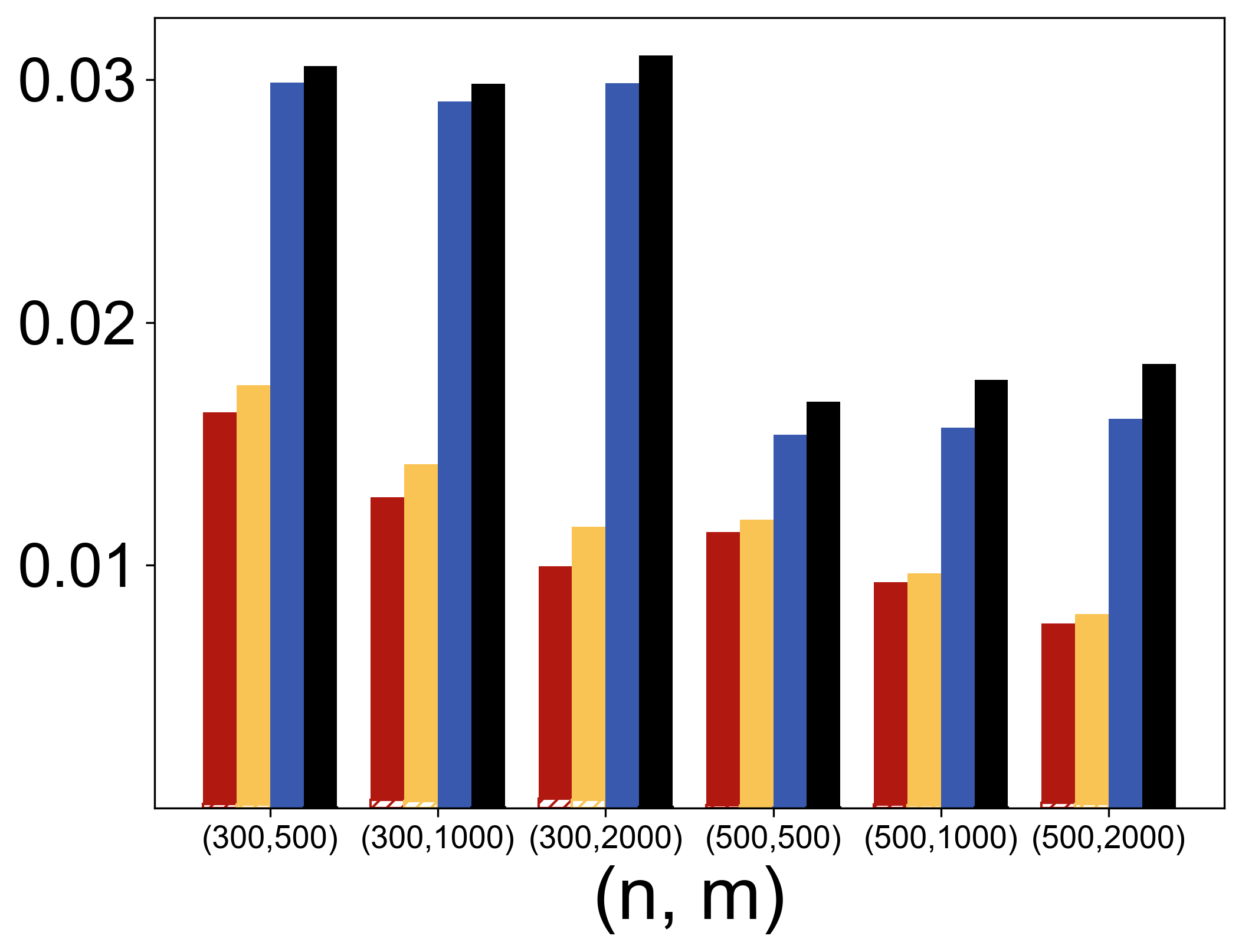
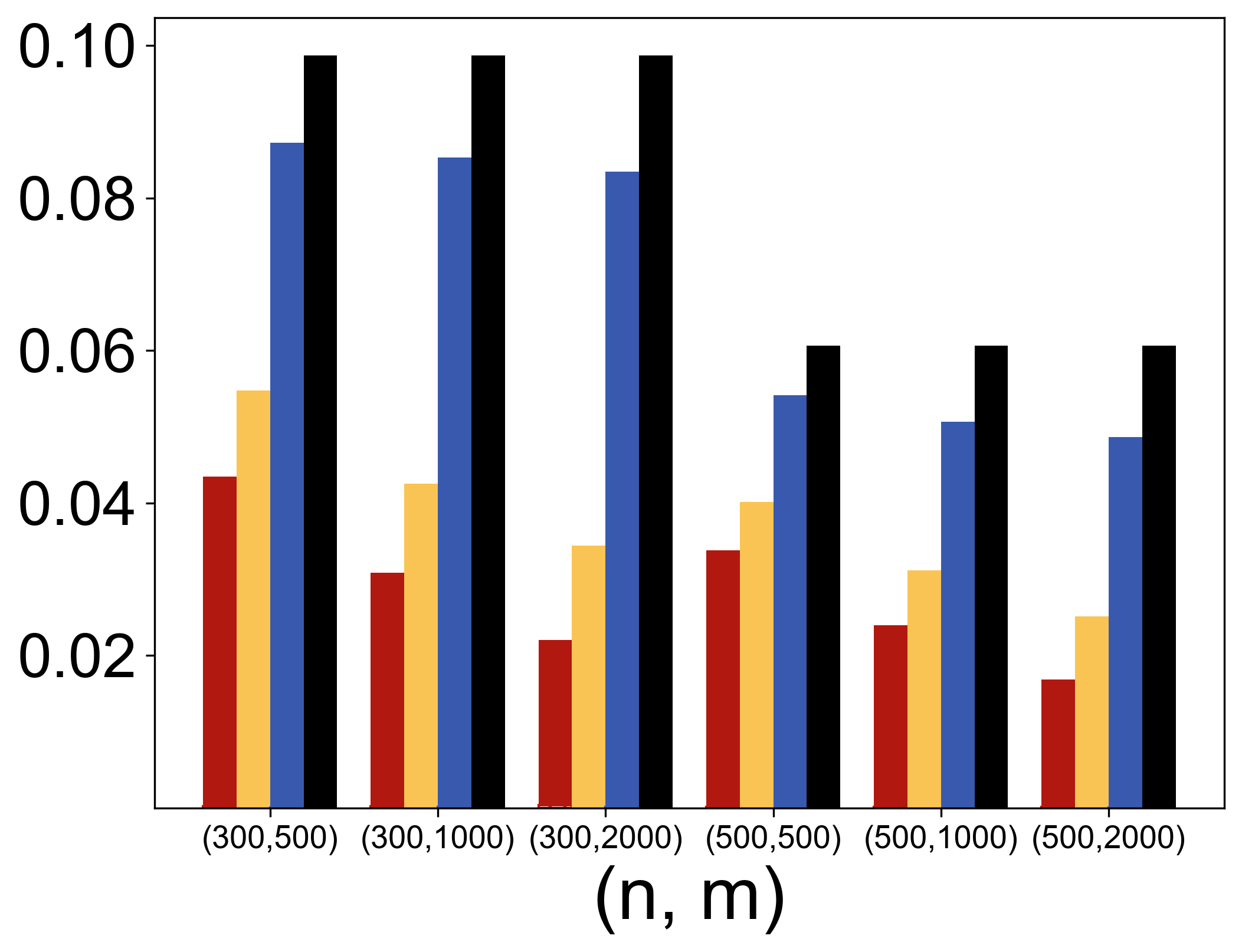
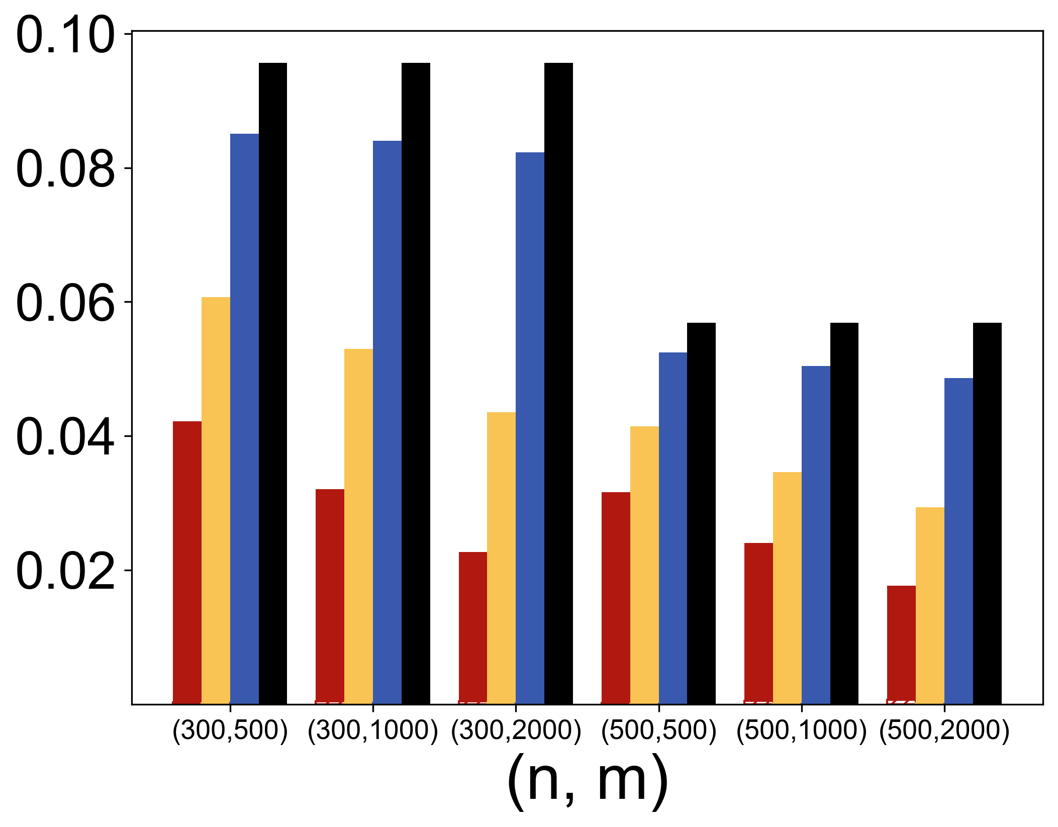
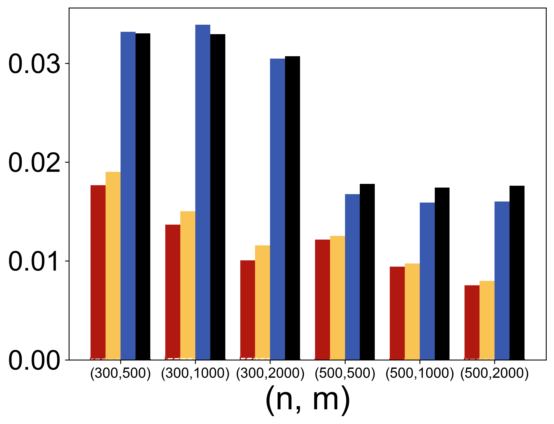
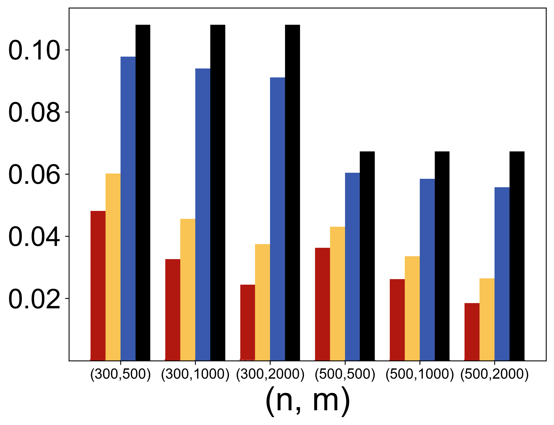
yielding at least configurations. For each configuration, we approximate the true via Monte Carlo integration using samples. Using replicates for each configuration, we compute estimates for , and use them to estimate the bias and mean squared error (MSE). Further experimental details are given in Appendix A.
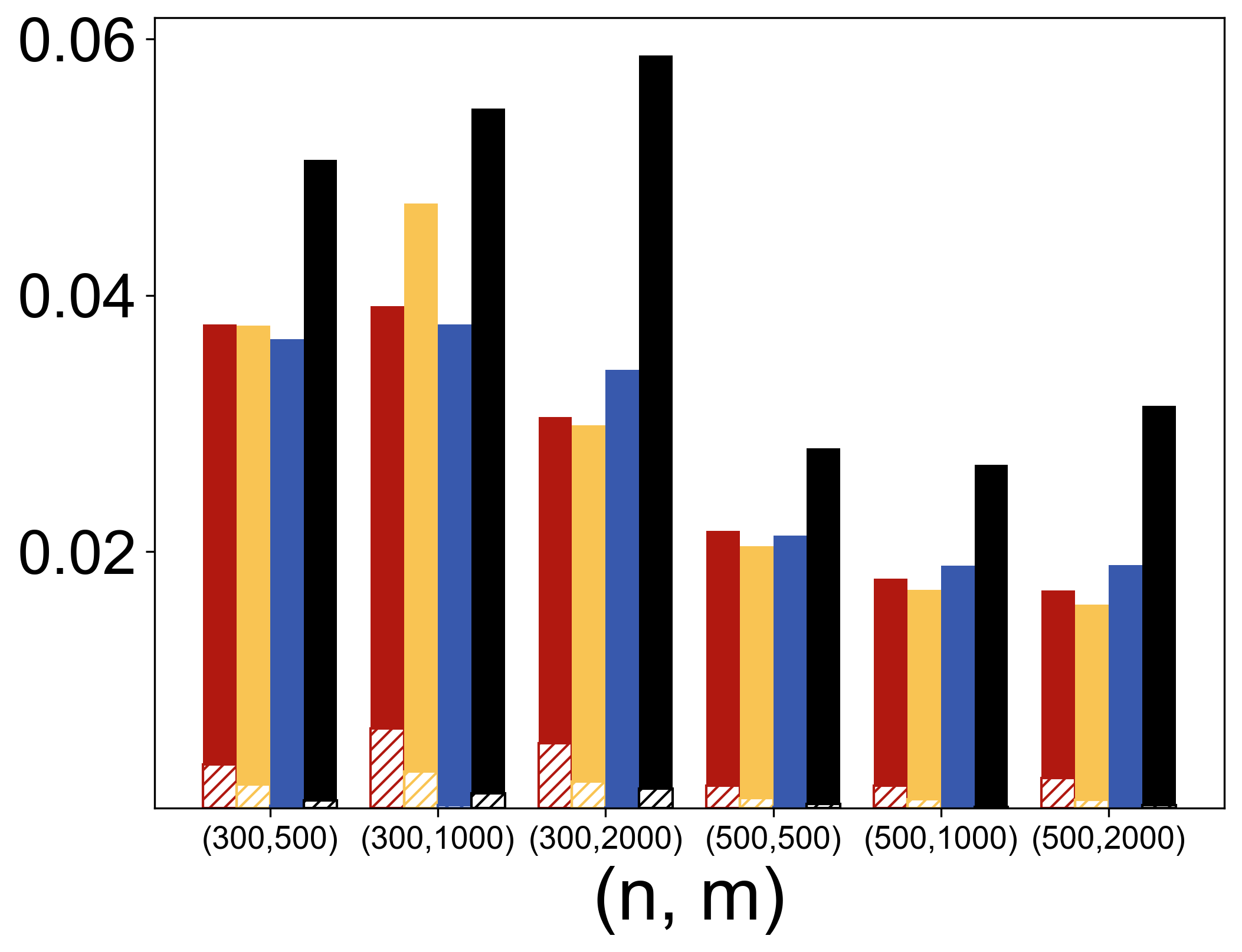
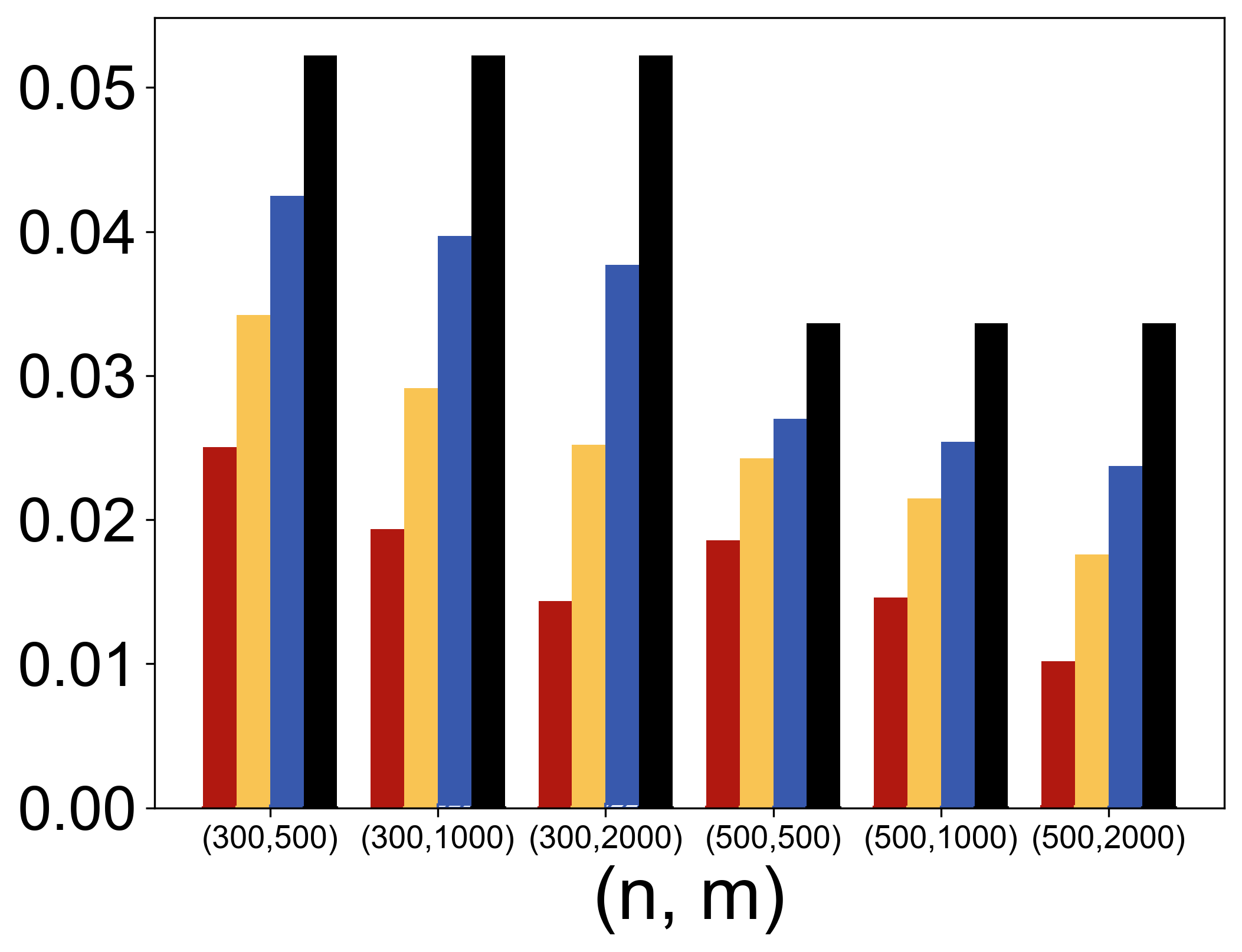
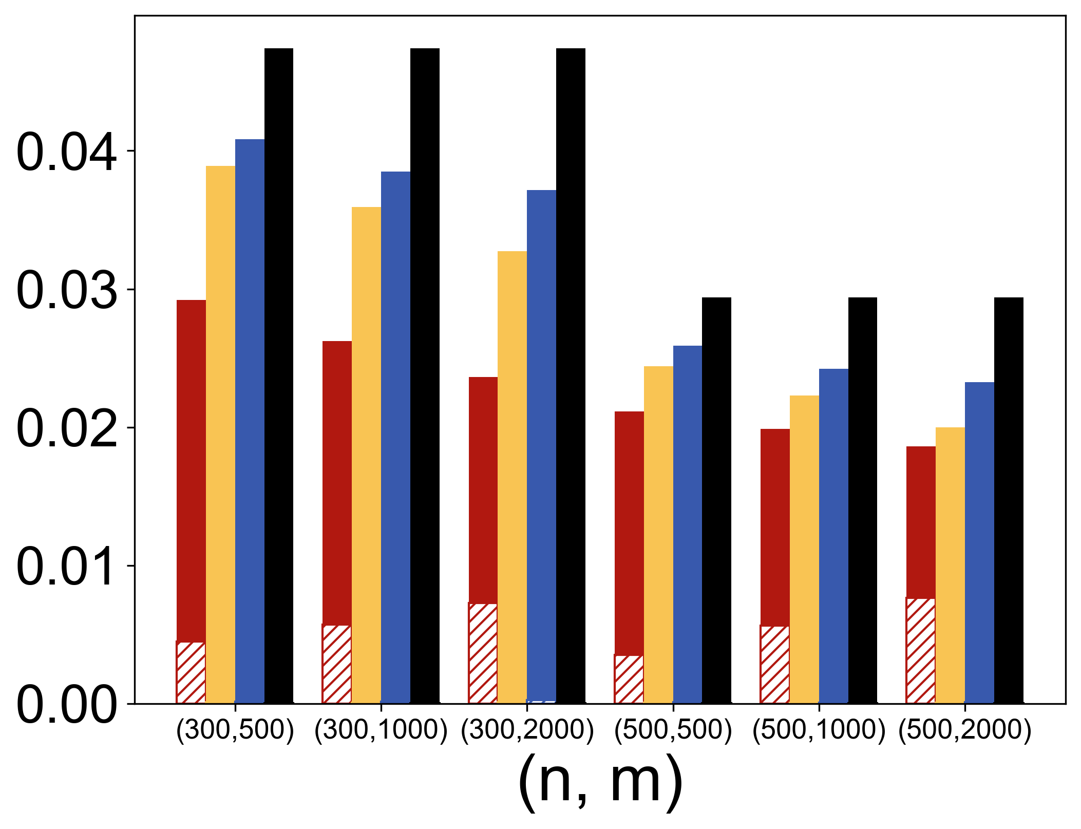
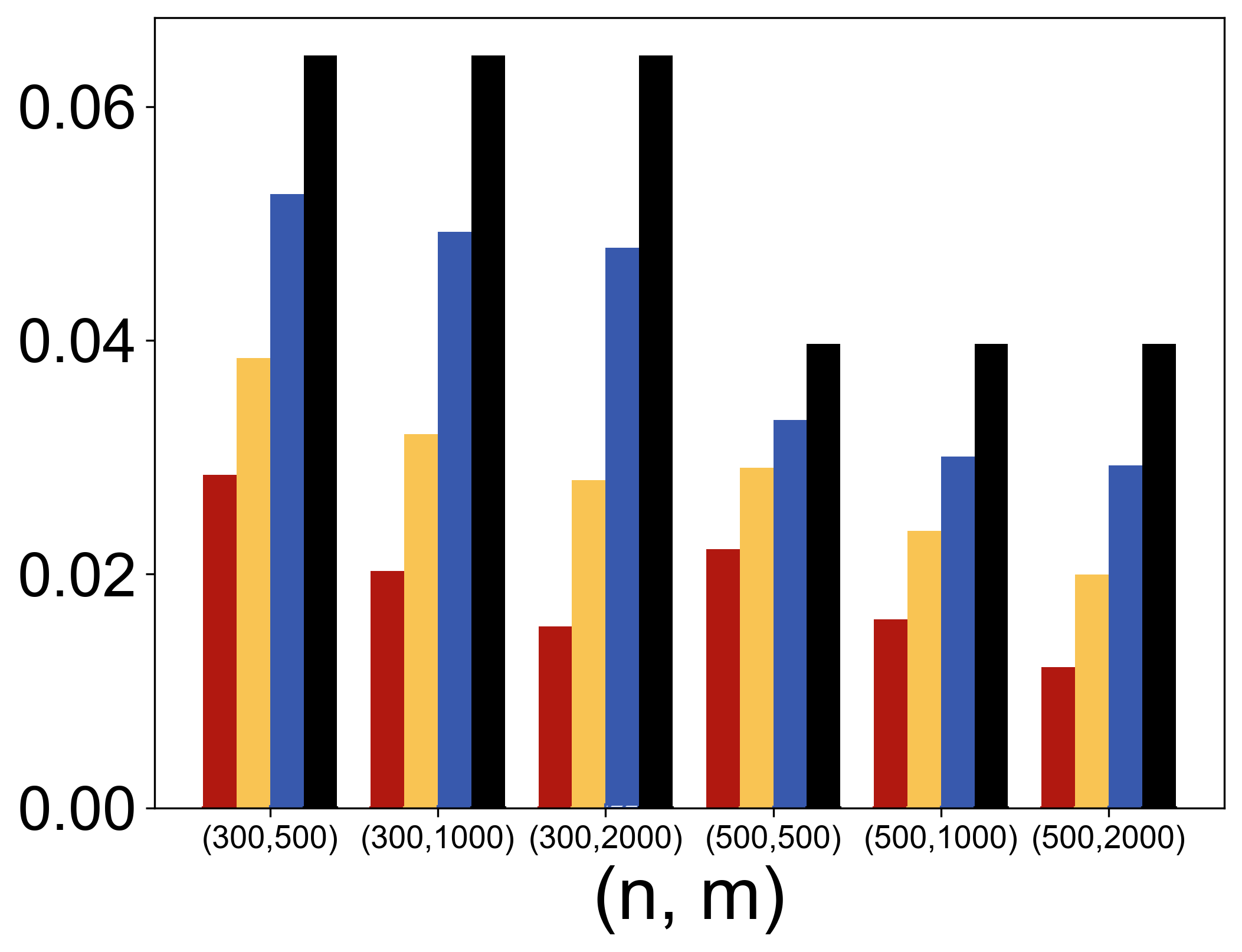
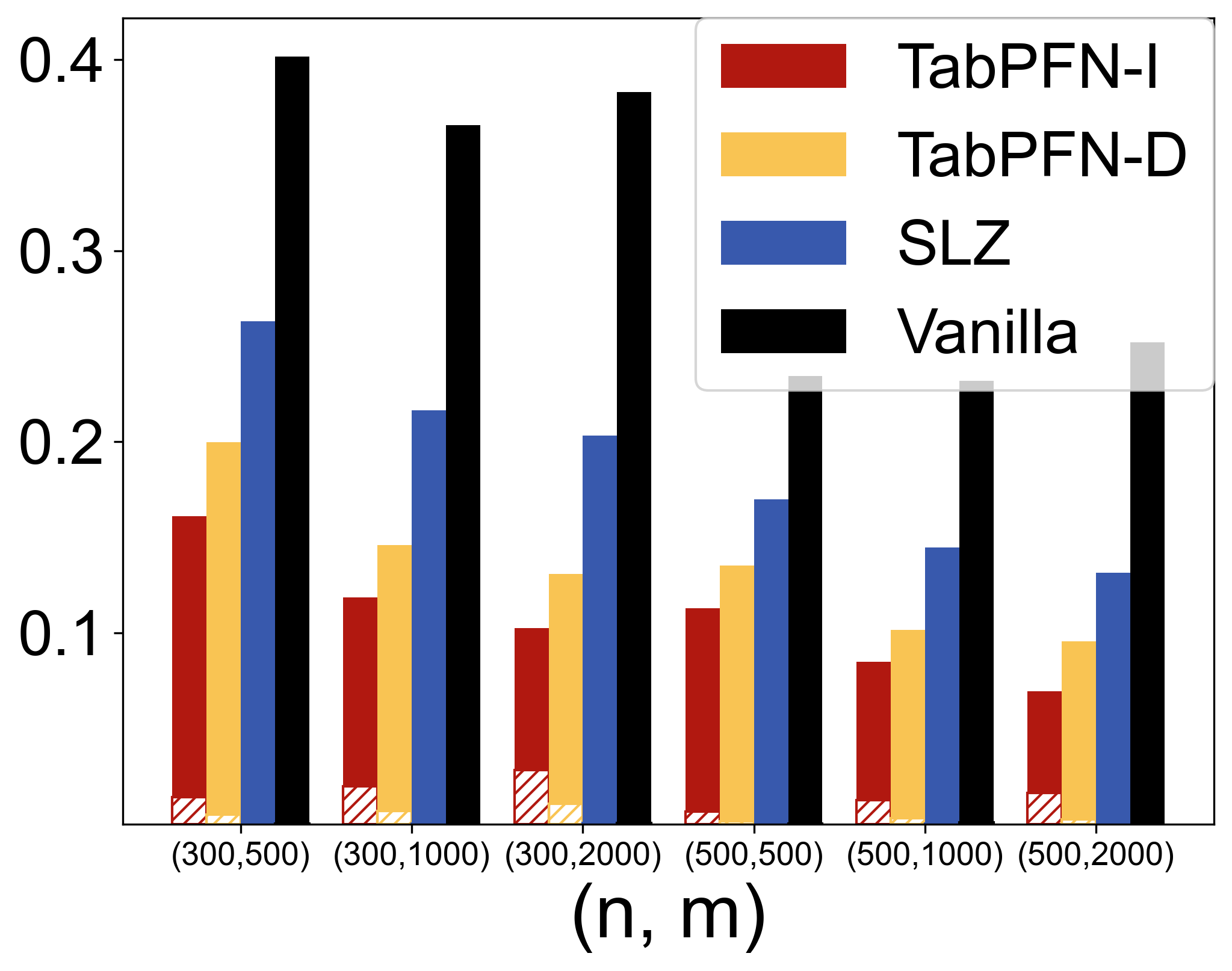
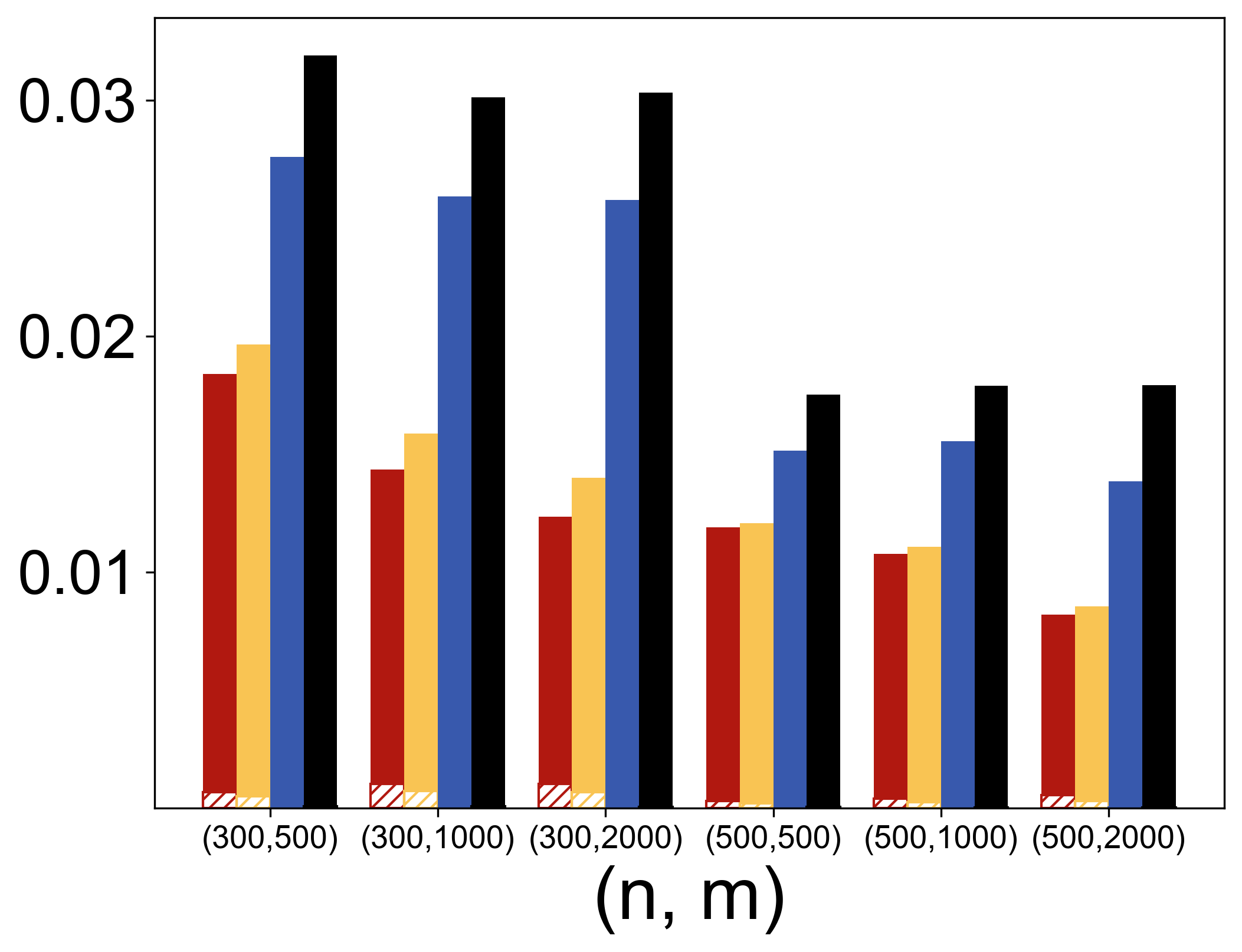
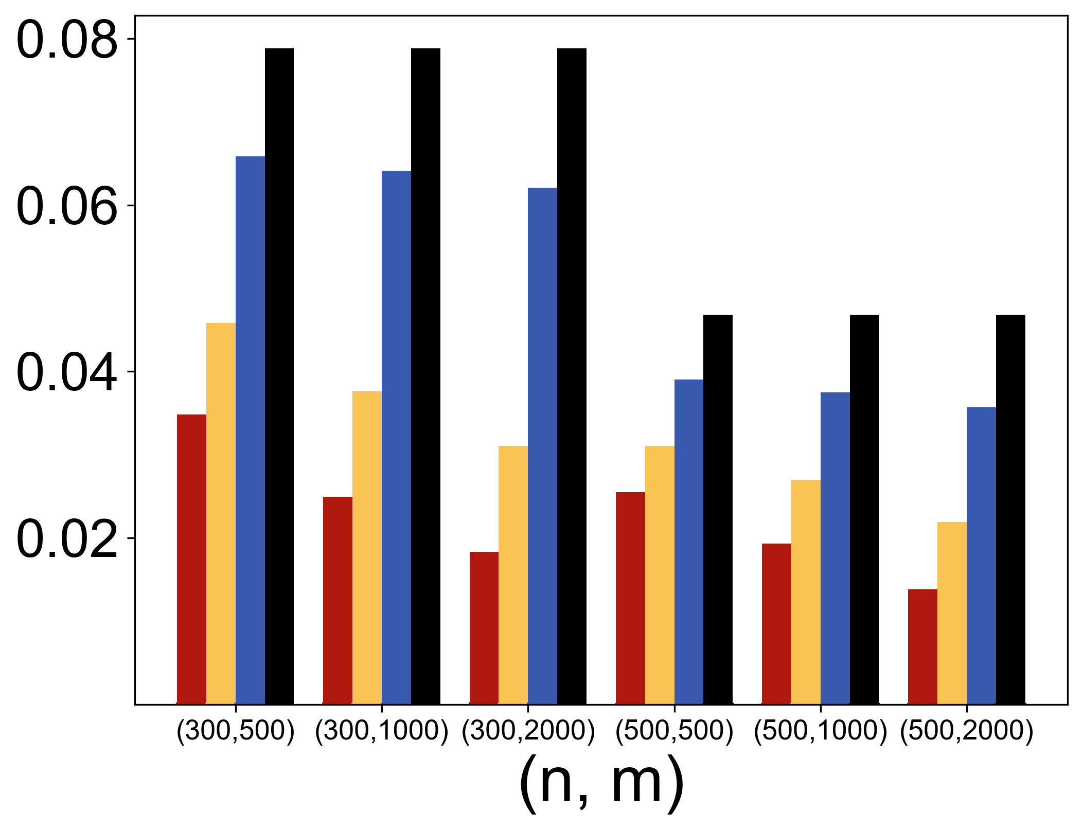
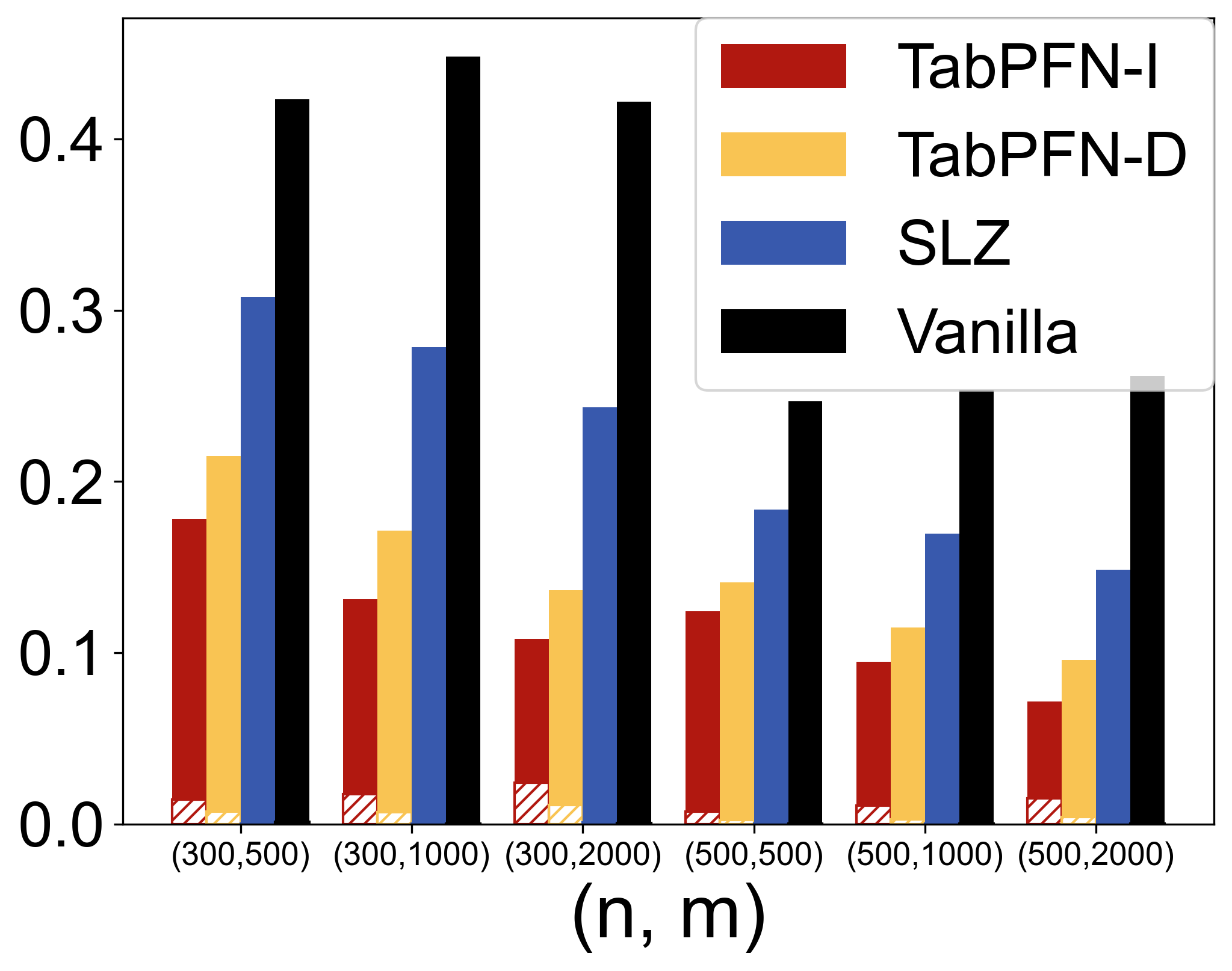
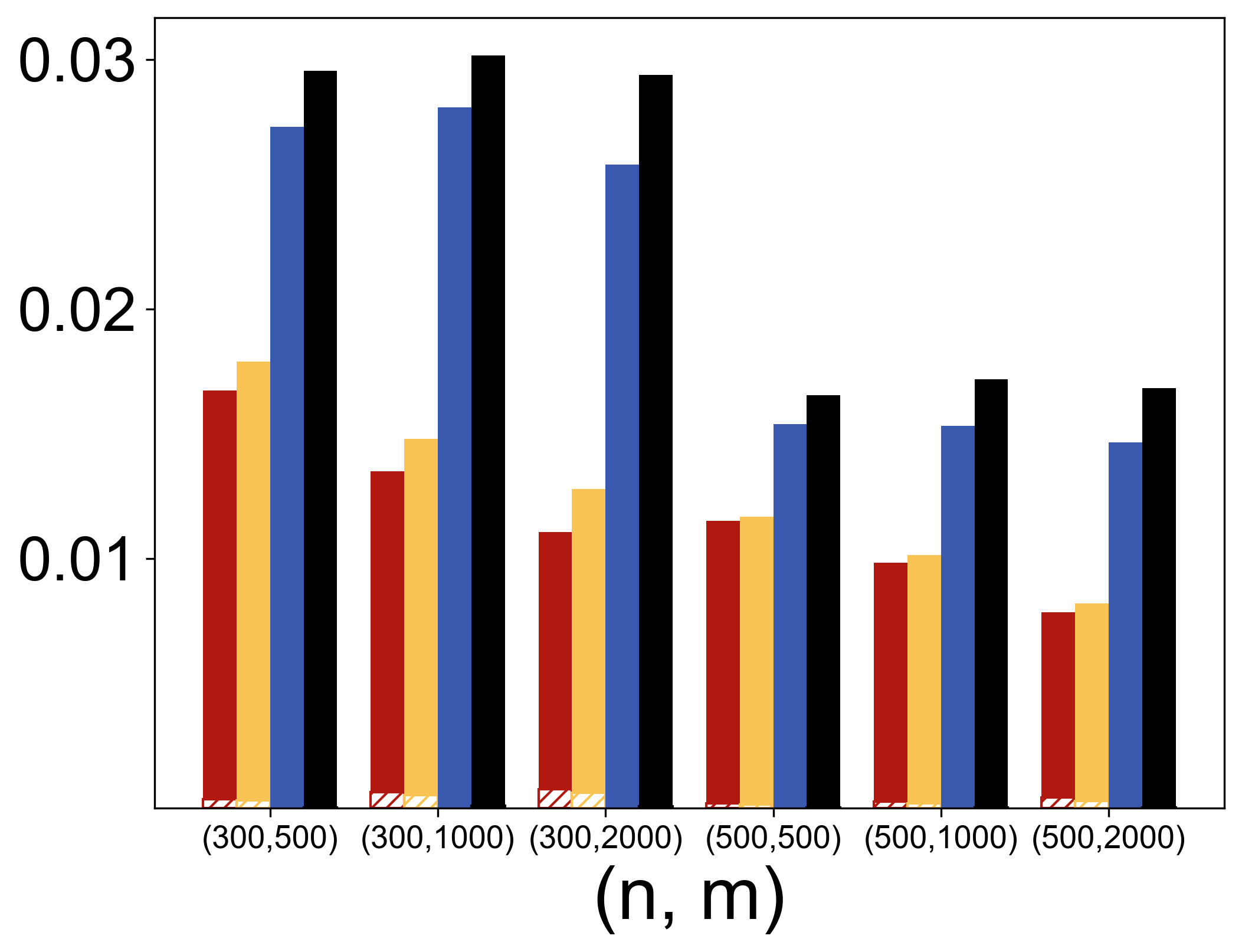
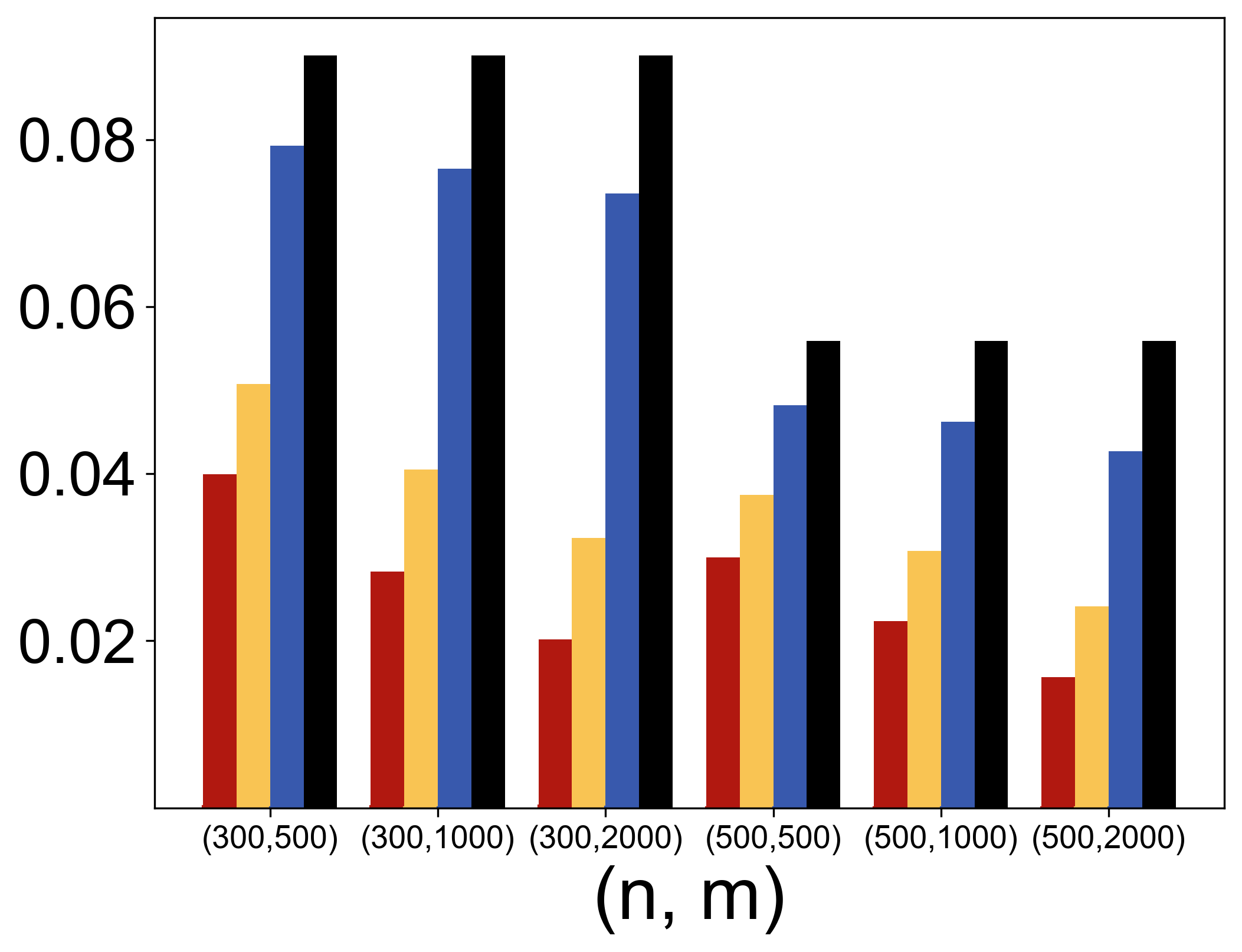
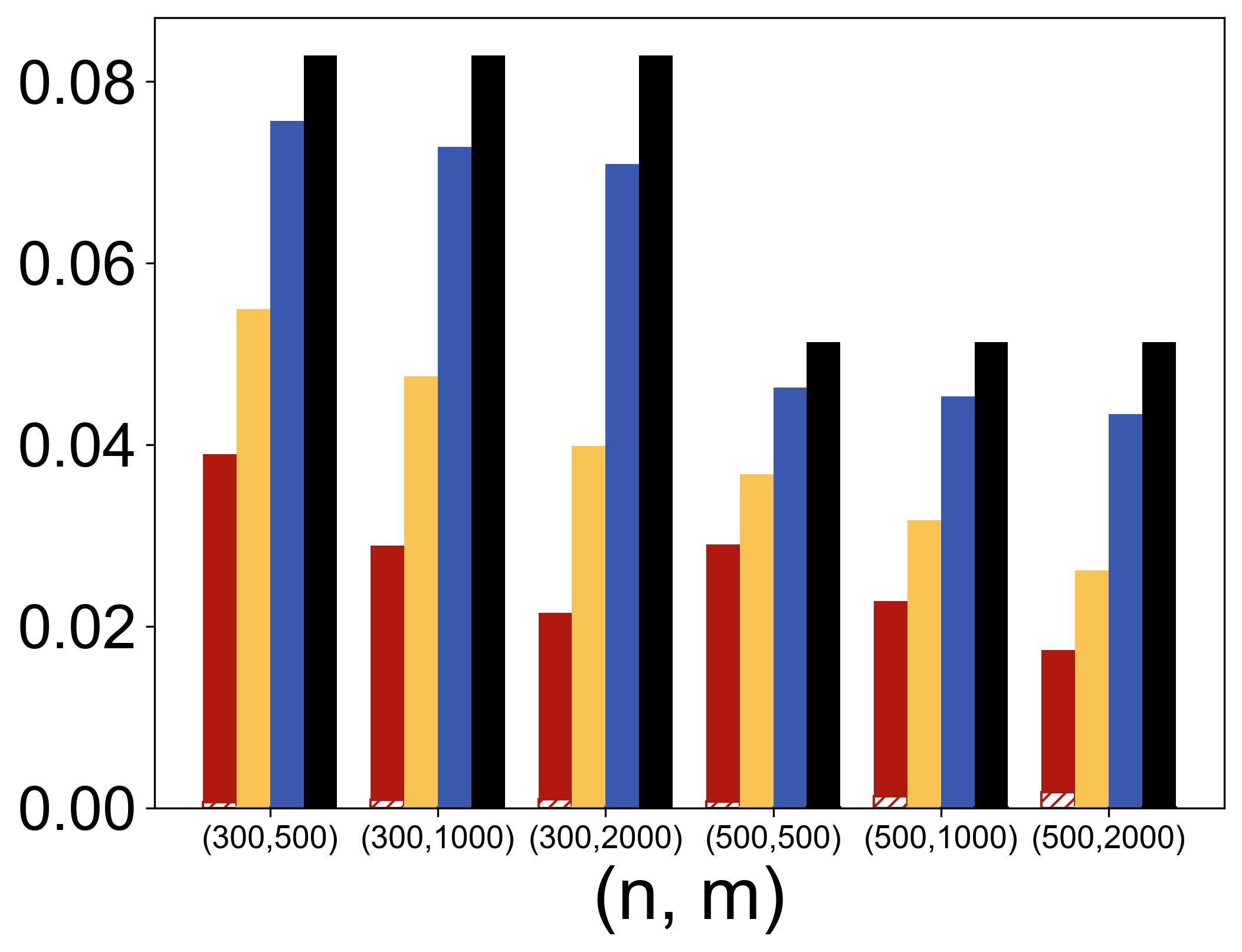
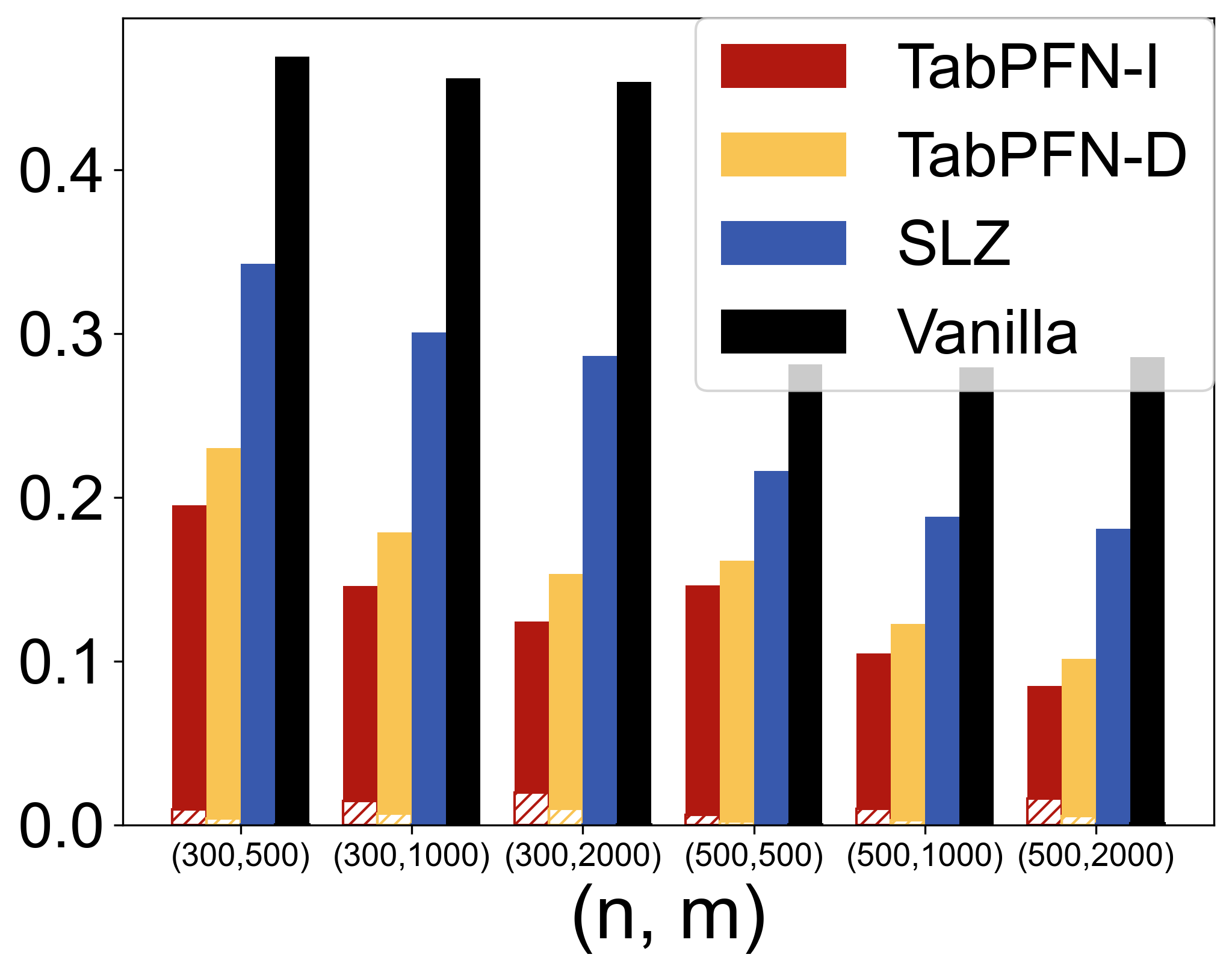
3.1.4 Results.
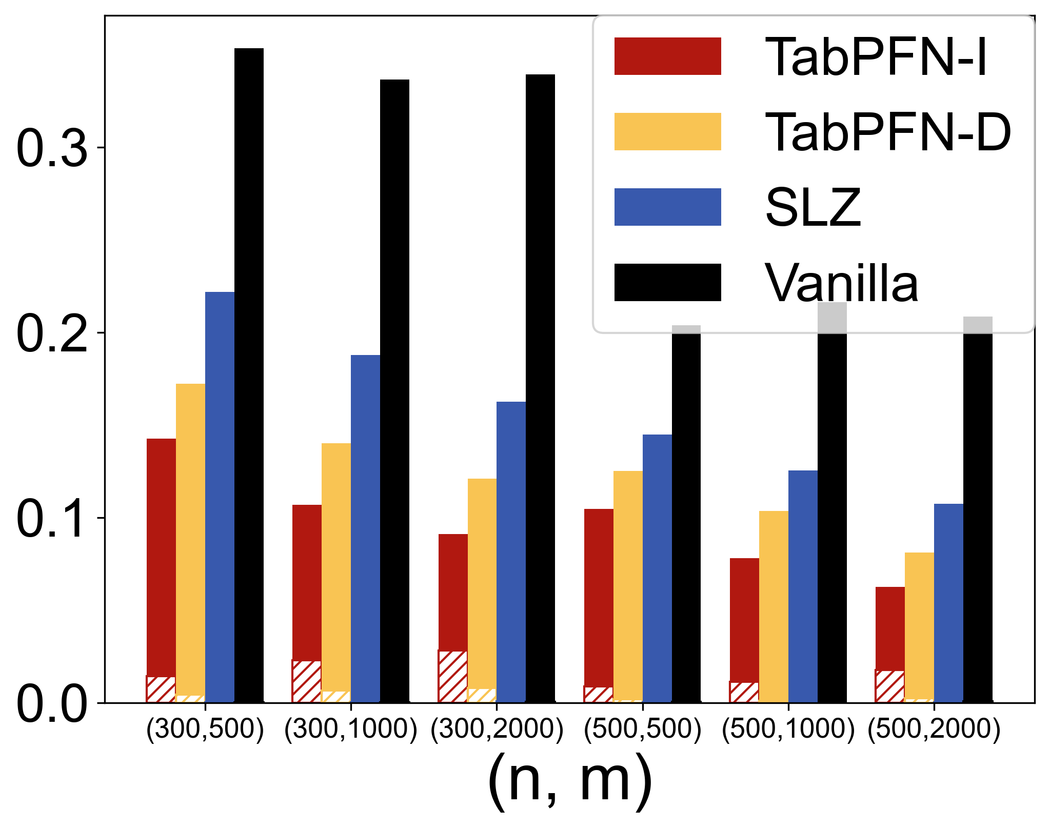
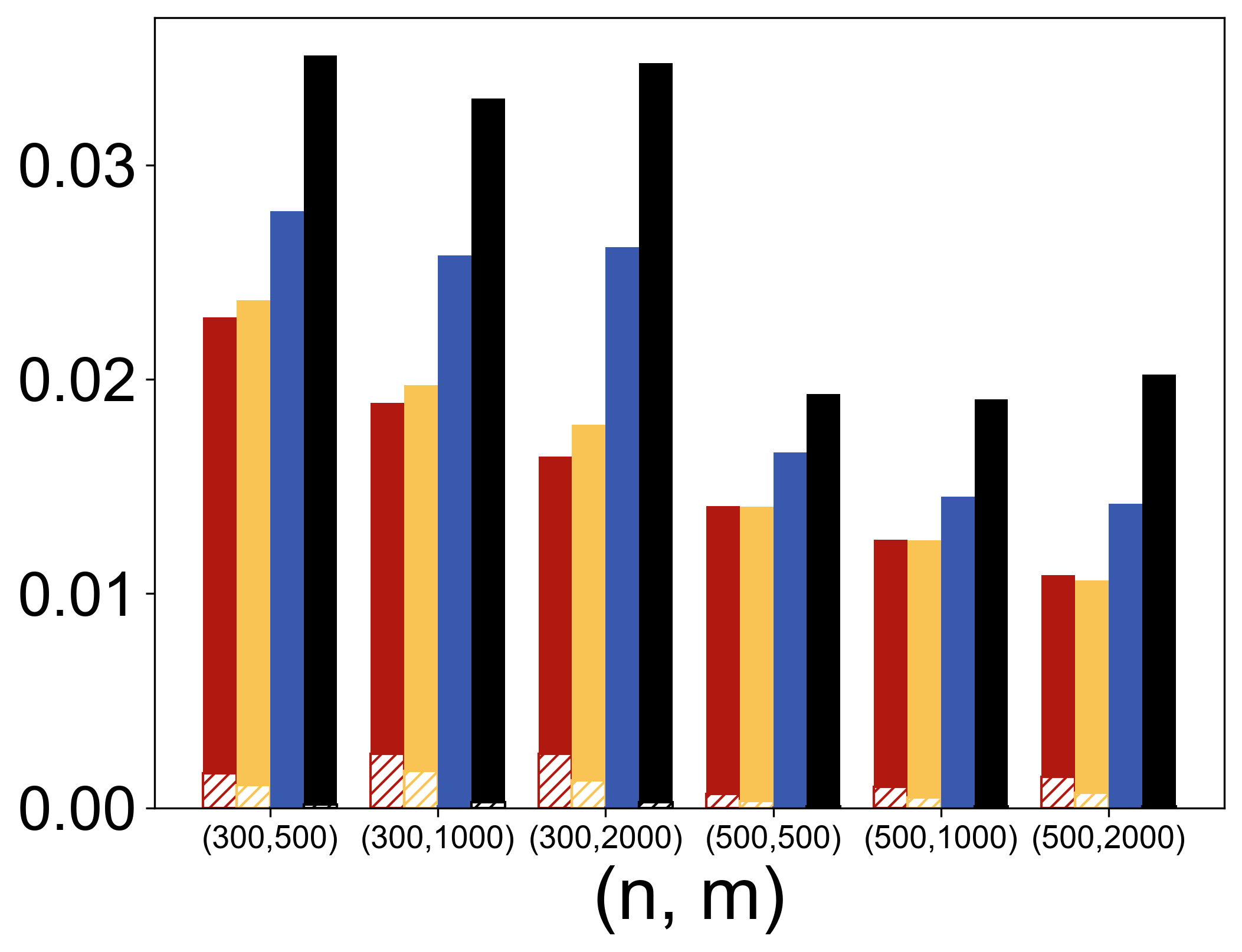
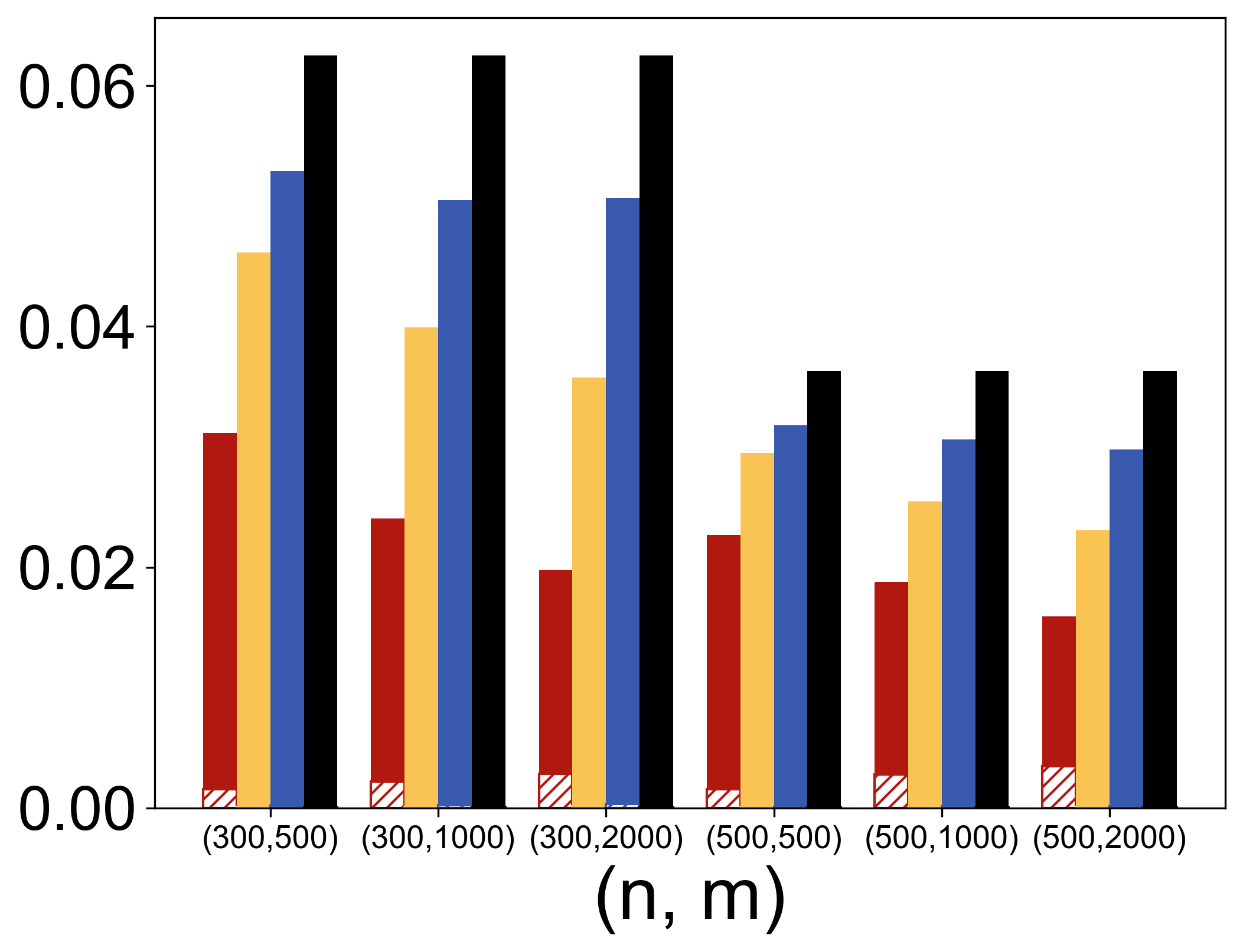
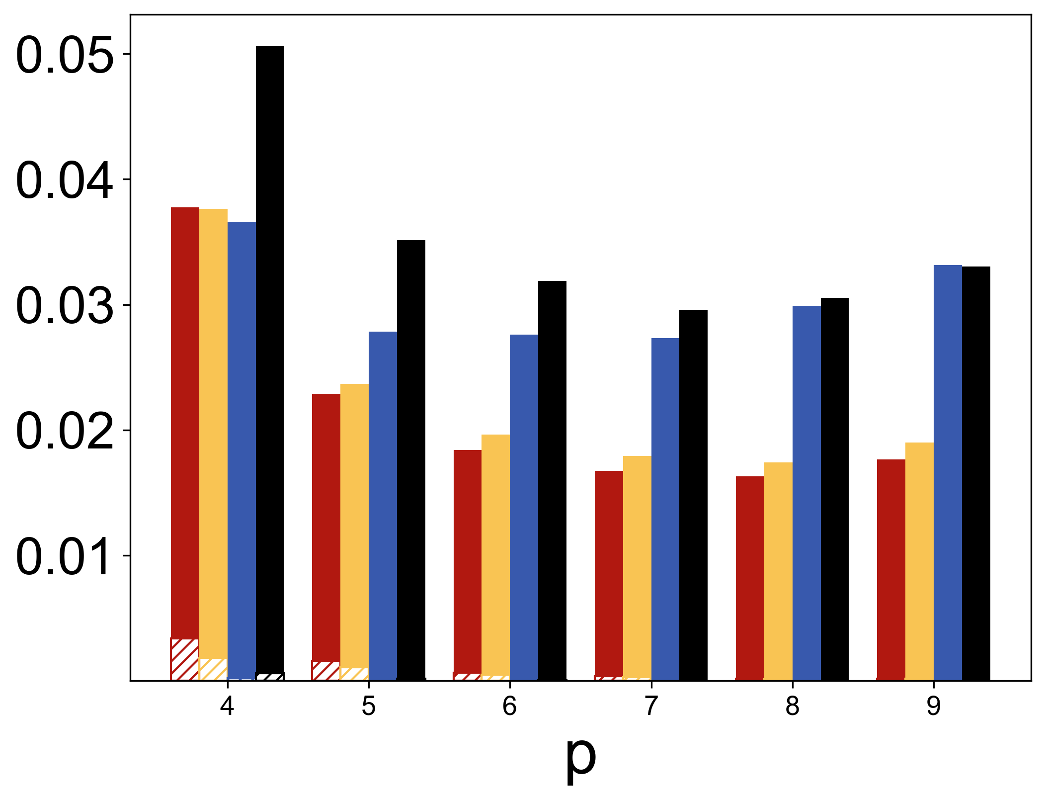
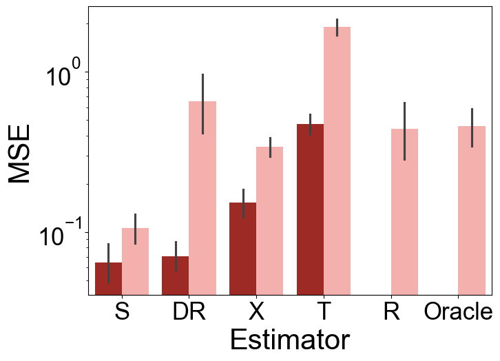
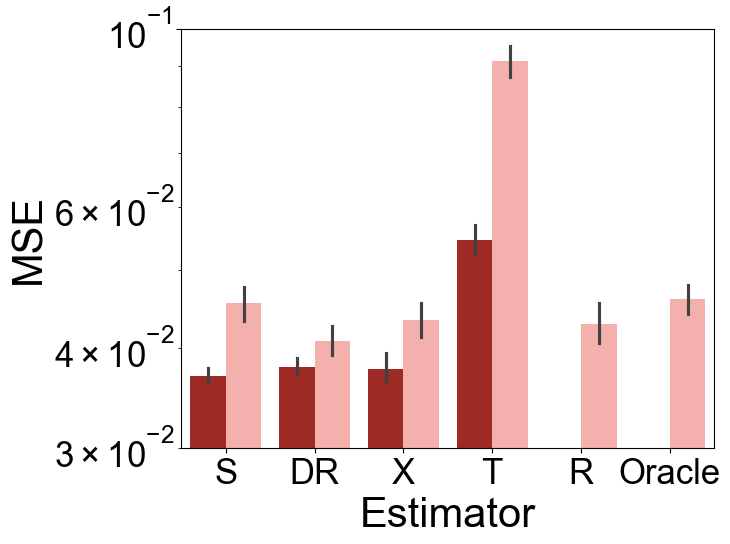
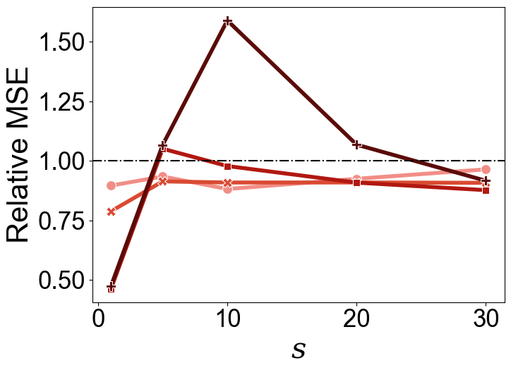
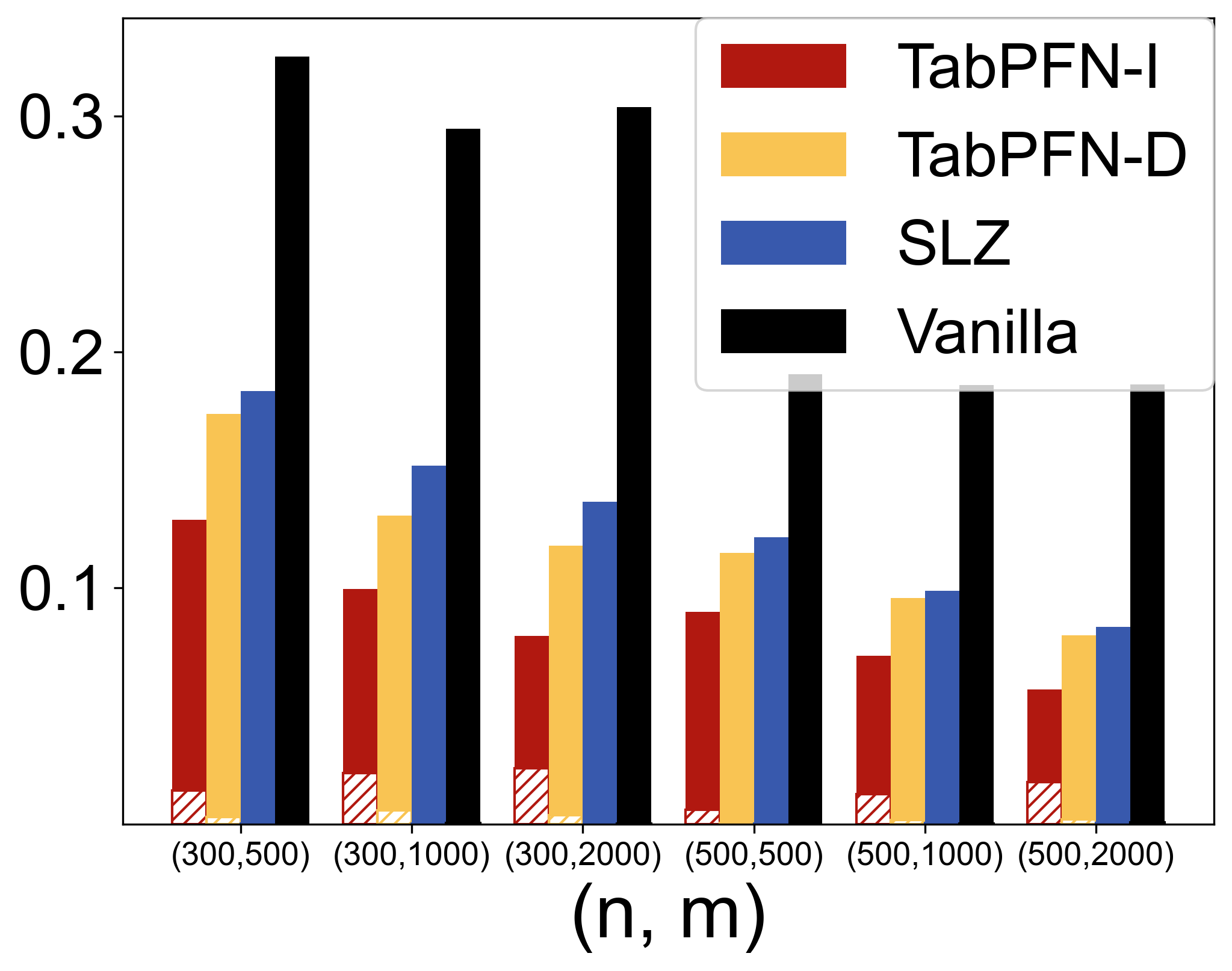
Representative results of our experiments are shown in Figure 1, with the complete set of results deferred to Appendix A. The top left, top right, and bottom left panels show MSE with respect to linear, logistic, and quantile regression respectively when , with various combinations of . In the bottom right panel, we show how the results for logistic regression vary with , observing that SLZ is only able to outperform the TabPFN approaches when . In general, we observe that TabPFN-I and TabPFN-D significantly outperform SLZ in terms of MSE. We also decompose MSE into squared bias (shaded bar) and variance (solid bar) for the four methods and observe that while TabPFN-I has larger bias than TabPFN-D (as well as the other two methods), it has significantly smaller variance, which leads to smaller MSE.
3.2 Case study II: heterogeneous treatment effects estimation
3.2.1 Problem and motivation.
While researchers were previously satisfied with estimating the average effect of a treatment–such as a drug, social intervention, or economic policy–across a population of interest, there has been rising interest in estimating heterogeneous treatment effects (HTE), that is, how different groups of individuals might benefit differentially from the same treatment. Accurate estimation of HTE can allow for personalized treatments, which may lead to better outcomes.
HTE is usually quantified via the Neyman–Rubin potential outcomes framework [35]. We consider IID samples from a population, where is a -dimensional feature vector, is a binary treatment assignment indicator, and and are potential outcomes. The observed outcome is . Define the response functions under control and treatment respectively as
and the conditional average treatment effect (CATE) function as
The propensity score is defined as . In contrast to the average treatment effect (ATE), defined as , the CATE is able to capture HTE and is hence our estimand of interest.
3.2.2 State-of-the-art.
Many methods have recently been proposed to estimate the CATE under the assumption of ignorability (). Most but not all of these methods can be subsumed under Künzel et al. [24]’s framework for “meta-learners”, which they defined as “the result of combining supervised learning or regression estimators (i.e., base learners) in a specific manner while allowing the base learners to take any form”. These include:
-
•
S-Learner: (a) Form an estimate for the function by jointly regressing on and ; (b) Set .
-
•
T-Learner: (a) Form estimates for and by regressing on within the control and treatment groups respectively; (b) Set .
-
•
R-Learner [28]: (a) Form estimates for and for ; (b) Compute residuals , ; (c) Solve
(3) -
•
DR-Learner [22]: (a) Form estimates for , for , and for ; (b) Compute doubly robust pseudo-outcomes using these models444; (c) Form an estimate for by regressing on .
-
•
X-Learner [24]: (a) Form estimates for and for ; (b) Impute treatment effects: (treatment group) and (control group); (c) Form preliminary estimates for by regressing on for ; (d) Combine the two estimates via (typically ).
Foster and Syrgkanis [14] advocated for either the R-Learner or DR-Learner as, unlike the S-, T- and X-Learners, they satisfy Neyman orthogonality, which result in theoretically faster estimation rates so long as the base learners used to estimate the nuisance parameters (e.g. and ) satisfy certain convergence properties. In their numerical experiments, they used Wang et al. [42]’s AutoML algorithm555AutoML uses cross-validation and a smart exploration strategy to select from a collection of the most popular machine learning models and to tune their hyperparameters. as the base learner in the meta-leaner strategies detailed above, and showed that the R-Learner or DR-Learner indeed achieved better performance.
3.2.3 Experimental design.
We repeat Foster and Syrgkanis [14]’s experiments, but add TabPFN as a choice of base learner. We compare the five meta-learner strategies detailed above, together with an “oracle” comprising the R-Learner fitted with the true nuisance functions and . Note that the optimization problem (3) for the R-Learner is solved via weighted least squares. Since TabPFN currently does not support weighted loss minimization, this means that it cannot be used as a base learner for both the R-Learner and oracle methods. This results in 10 total estimators ( base learners × methods – exclusions). Throughout our analysis, we identify each estimator by its method followed by the base learner in parentheses (e.g., ‘S-Learner (TabPFN)’).
In each experiment, we generate a dataset according to the Neyman-Rubin model detailed above, with and for , where . We explore different configurations of the functions , and , but because of space constraints, present only the following two representative cases in the main paper:
-
•
Setup A: complicated and , but a relatively simple .
-
•
Setup E: large resulting in substantial confounding, discontinuous .
Complete specifications of the functional forms and other settings are given in Appendix B. We vary two key experimental parameters: the training set size and noise level . For evaluation, we generate a fixed test set of size and report the MSE of the estimated treatment effect function evaluated on the test set. The results are averaged over 100 replicates.
3.2.4 Results.
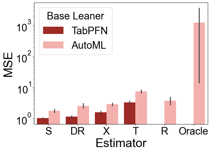
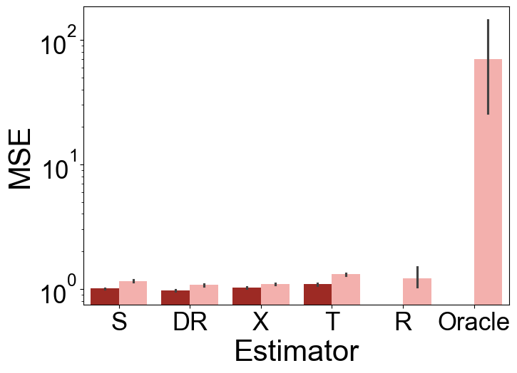
We display the results for Setup A and E in Figure 2 and defer the complete set of experimental results to Table 4 in Appendix B. Most strikingly, across all experimental settings, using TabPFN as the base learner in a meta-learner strategy greatly improves upon its AutoML counterpart. Second, despite its lack of Neyman orthogonality or double robustness, S-Learner (TabPFN) achieves the best accuracy in most settings and is among the top two performers in almost all settings. Our results stand in contrast to those of Foster and Syrgkanis [14] and the rest of the current HTE literature, which has tended to de-emphasize the role played by the base learner because the error it accrues when estimating the nuisance parameters becomes second-order for the R- and DR-Learners under what they consider to be relatively mild conditions. The superior performance of S-Learner (TabPFN) shows that this asymptotic regime is not attained, even under relatively simple simulation settings, and that the choice of base learner can be equally important as the choice of metalearner framework. Indeed, the superior regularization of TabPFN compared to other regression estimators may have a special synergy with the S-Learner strategy, resulting in its superior accuracy, especially in low sample size and signal-to-noise ratio (SNR) settings.
3.3 Case study III: prediction under covariate shift
3.3.1 Problem and motivation.
In regression and classification problems, covariate shift refers to the scenario where the marginal covariate distribution differs between training and test datasets, while the predictive distribution remains the same. This distributional mismatch frequently arises in real-world applications—for instance, due to outdated training data or sampling biases between datasets. Since covariate shift can substantially degrade model performance, it has become an active area of research [32, 31, 43].
More precisely, we observe a training dataset comprising IID observations from a source distribution and wish to predict the responses on a test dataset comprising IID observations from the target distribution , with accuracy evaluated via prediction MSE. Furthermore, and are usually unknown and have to be estimated from data.
3.3.2 State-of-the-art.
Classical approaches to address covariate shift make use of importance weighting techniques. More recently, the problem has been studied under the assumption that the regression function has bounded norm in a reproducing kernel Hilbert space, in which case kernel ridge regression (KRR) with a carefully tuned regularization parameter was shown to achieve optimal rates, whereas a naïve, unadjusted estimator is suboptimal [25]. Wang [41] introduced a method based on “pseudo-labeling” (PL) for selecting , claiming that it improves upon Ma, Pathak and Wainwright [25]’s work by relaxing certain distributional assumptions. Specifically, PL fits KRR on the first half of and uses the fitted model to impute labels for an auxiliary unlabeled dataset drawn from . It then fits a collection of KRR models with different parameters on the second half of and uses with the imputed labels to select the best-performing model.
3.3.3 Experimental design.
We repeat Wang [41]’s experiments, but add a simple comparator approach which directly fits a model on using TabPFN and does not make any adjustment. In addition to PL, the following methods were used as comparators:
-
•
Naive: Fit a gradient boosting regression model on , tuned using five-fold cross-validation.
-
•
Importance-Weighted (IW): Fit a gradient boosting regression model on similarly to the naive approach, but with the loss function weighted by the true density ratio .
-
•
Wang-Oracle: A variant of PL where the true conditional means are used for instead of imputed values. This serves as an oracle benchmark within Wang [41]’s framework.
We consider univariate covariate distributions that are Gaussian mixtures. The training and test distributions have the same components but differ in their mixing weights:
The response variable follows , where we investigate five distinct mean functions:
-
(i)
;
-
(ii)
;
-
(iii)
;
-
(iv)
, and ;
-
(v)
.
In each experiment, we generate training and test datasets as described above, with the size of the test set fixed at , while we vary the training set size . The results are averaged over 500 replicates.
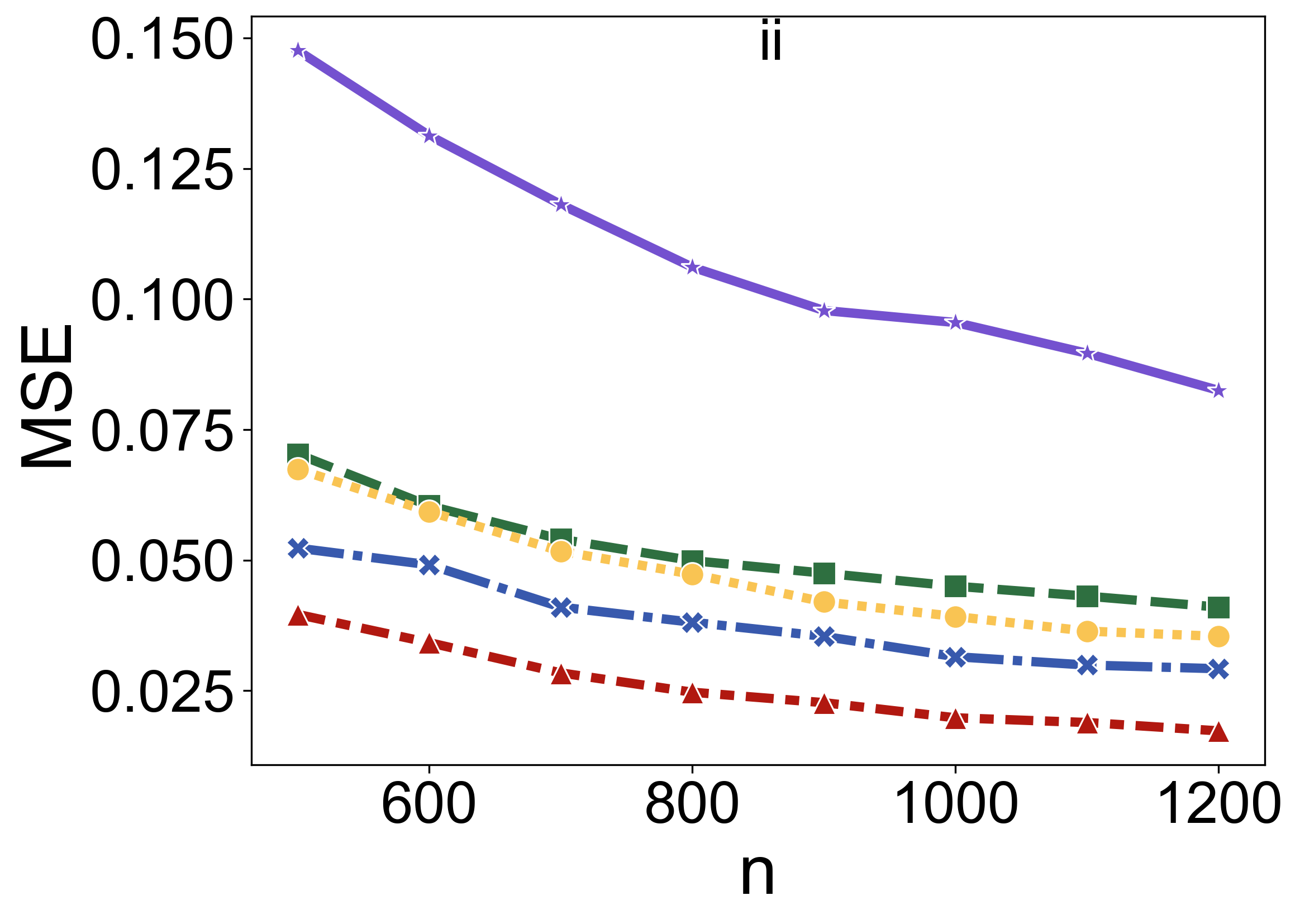
3.3.4 Results.
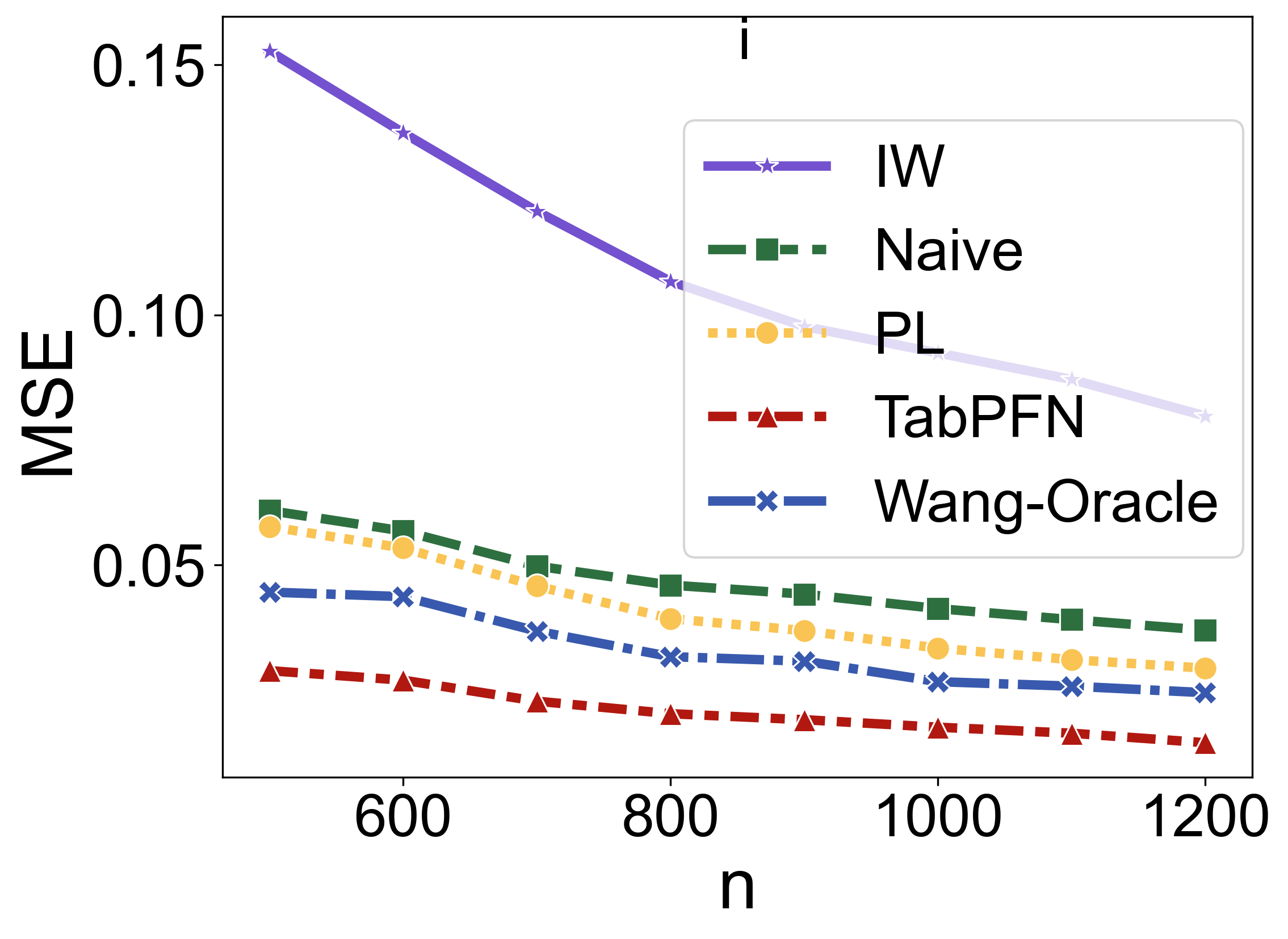
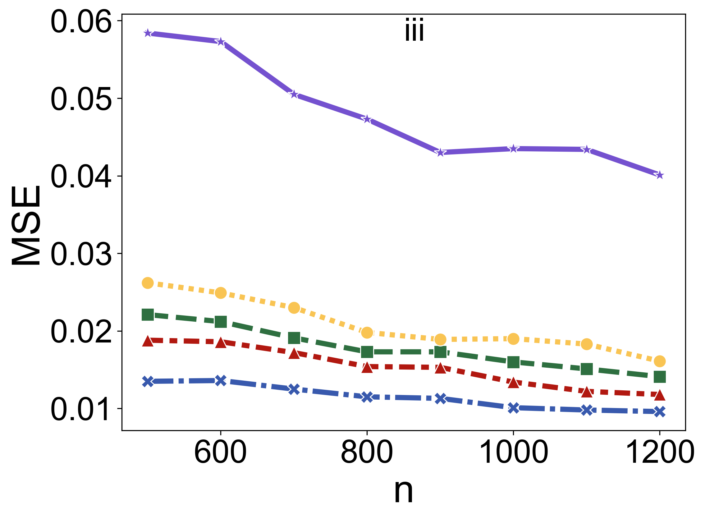
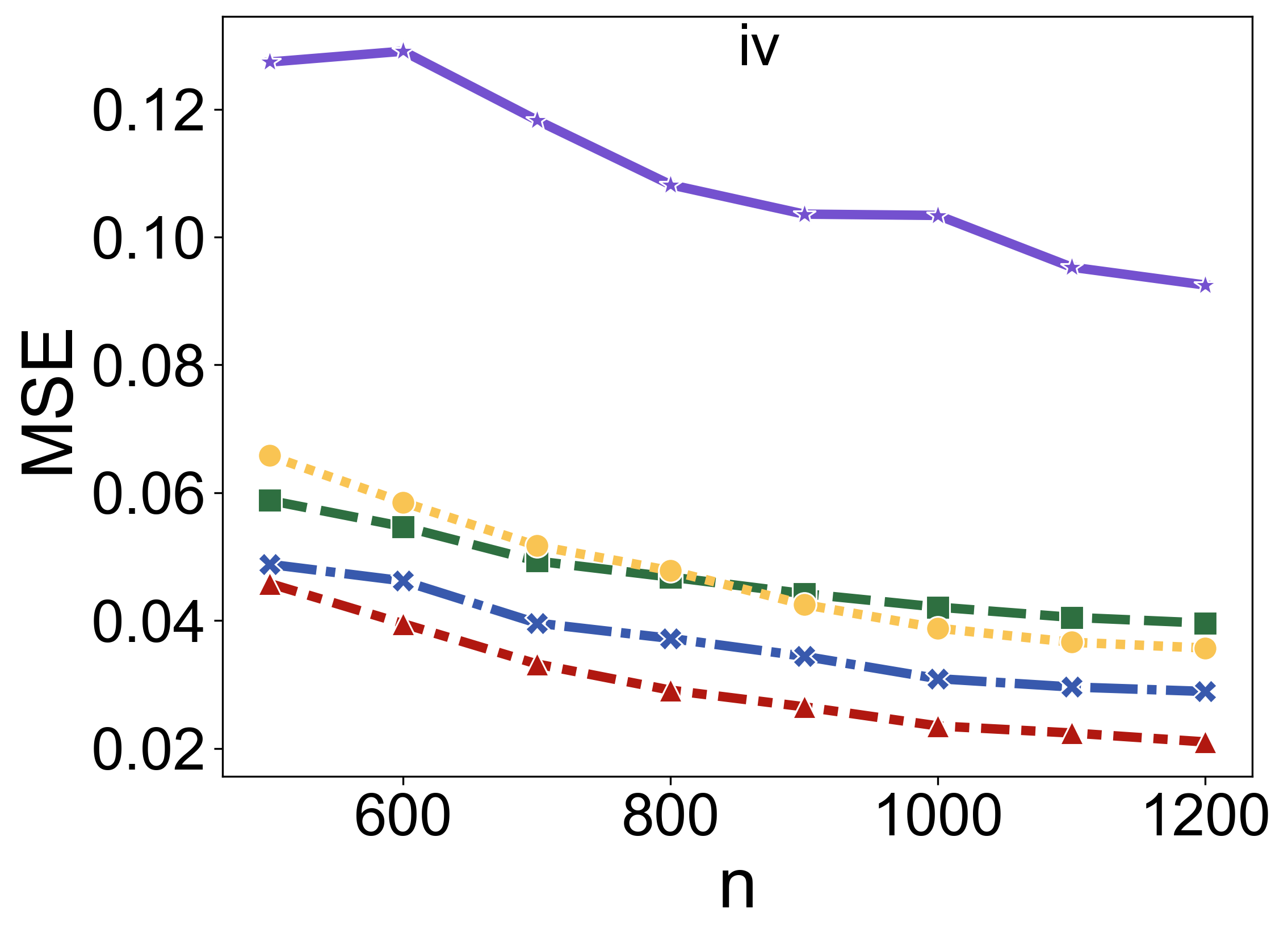
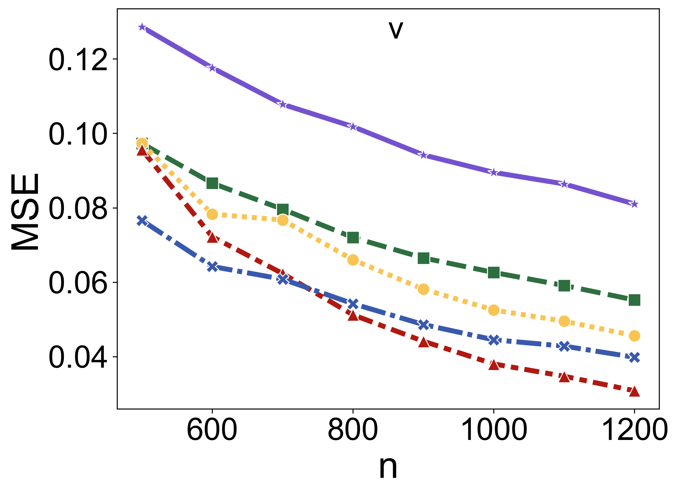
Figure 3 shows the prediction MSE as a function of for all five methods, with respect to the mean functions (i), (iii), (iv), and (v) (results for setting (ii), which shows similar patterns to (i), are provided in Appendix C). We observe that TabPFN consistently outperforms the PL method, even matching or exceeding the oracle method’s performance at larger sample sizes (), in all settings apart from (iii). This is despite TabPFN not making use of the auxiliary information in required by PL and the oracle method.
4 TabPFN inductive biases
A classical statistical method makes explicit assumptions about how data is generated, with its prediction performance suffering degradation when those assumptions do not hold. Conversely, when the data contains structure that is not exploited by the method, such as when applying smoothing splines to data generated from a linear model, the prediction performance of the method can be relatively inefficient. Machine learning methods, such as tree-based ensembles and neural networks, are algorithmically defined, which means that these assumptions are implicit rather than explicit. These implicit assumptions are referred to as the method’s inductive bias. Uncovering the inductive biases of ML methods is an active and important area of research, as it tells us when we can expect a given method to do well and when it might perform poorly.
In this section, we attempt to investigate TabPFN’s inductive biases via a collection of numerical experiments. Our takeaways are that
-
•
In low dimensions, TabPFN seems similar to Gaussian process regression in its ability to adapt flexibly to any functional form, but differs notably in its manner of extrapolation, ease of fitting step functions, and conservativeness at fitting quickly-varying functions.
-
•
TabPFN can outperform LASSO at high sparsity and low SNR settings by avoiding excessive shrinkage of relevant feature coefficients. On the other hand, it generally performs even worse than LASSO for dense linear regression for features.
-
•
TabPFN is able to break a robustness-efficiency trade-off in classification: It is simultaneously robust to label noise (a type of model misspecification), while being as efficient as linear discriminant analysis (LDA) when it is correctly specified.
4.1 Interpolation and extrapolation
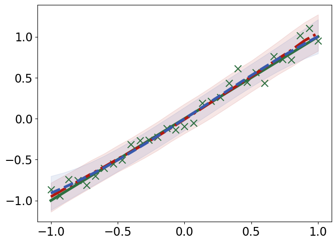
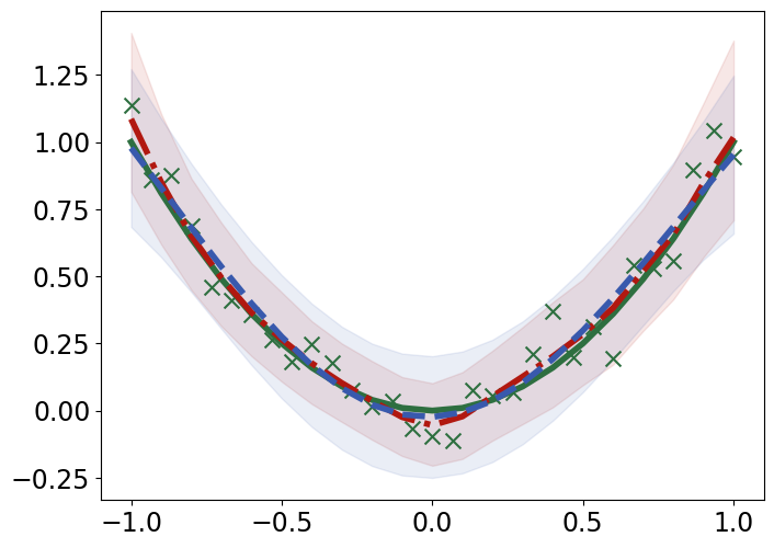
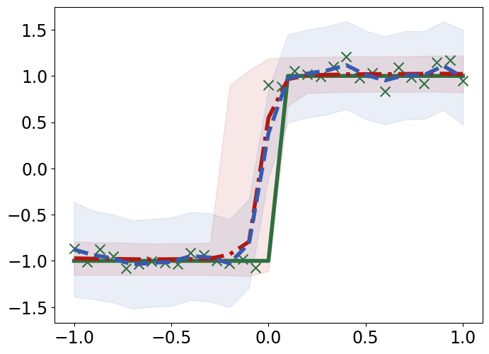
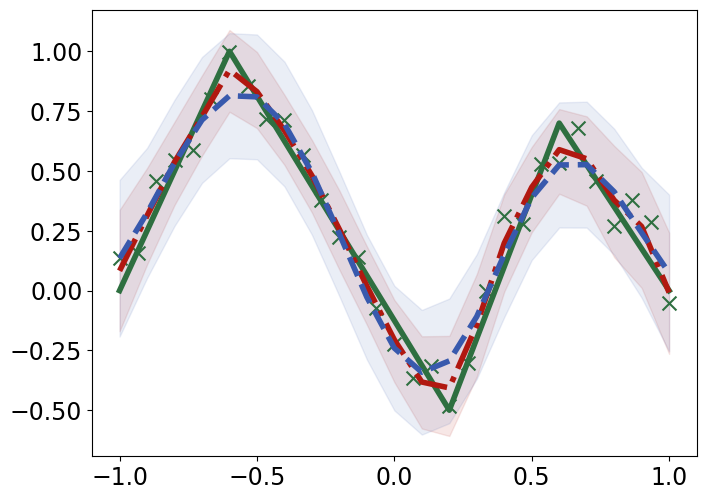
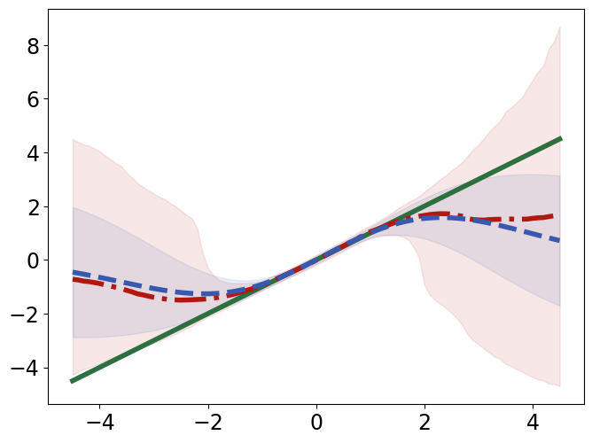
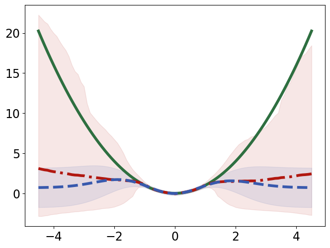
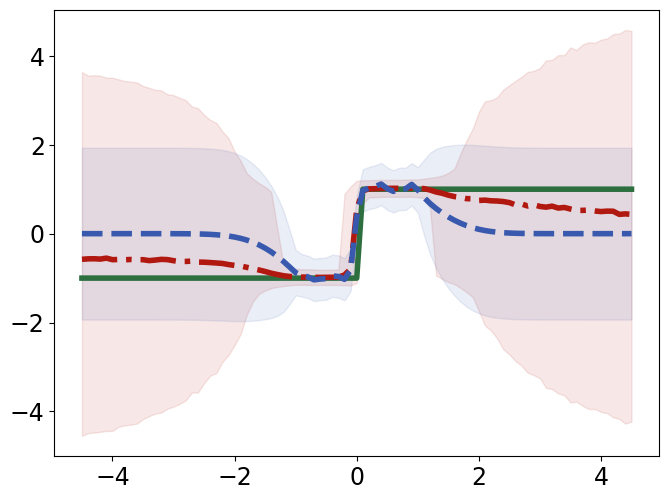
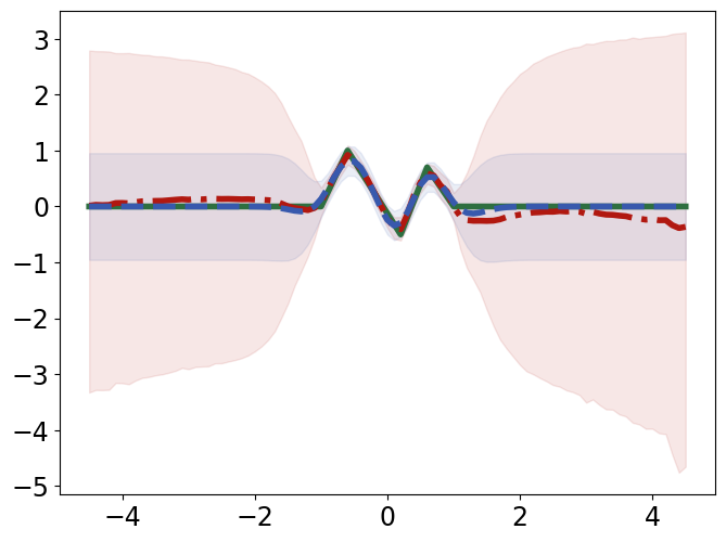
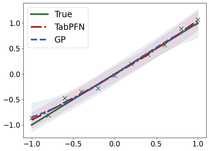
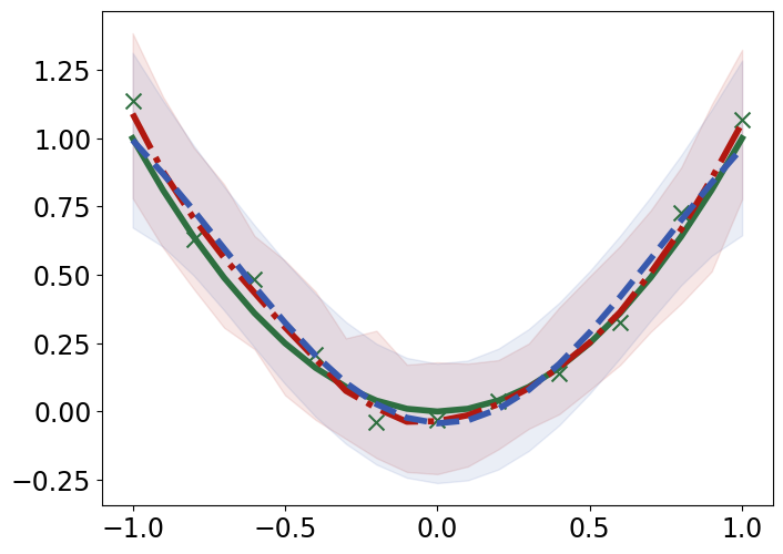
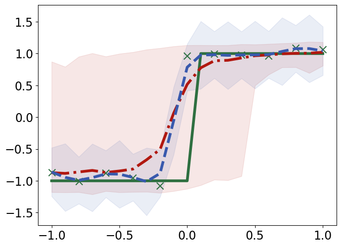
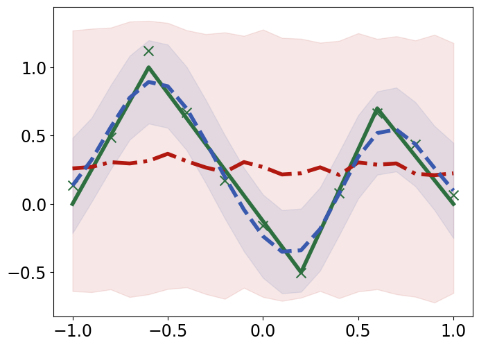
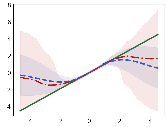
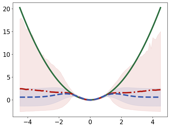
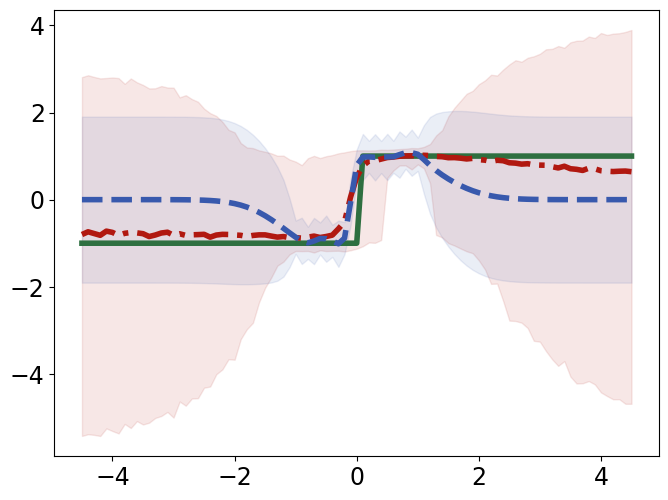
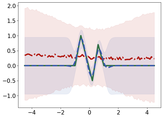
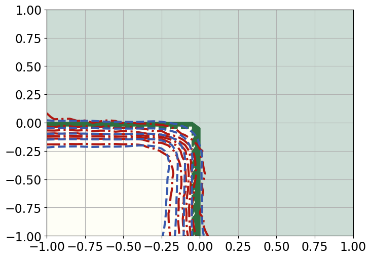
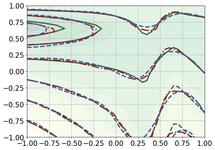
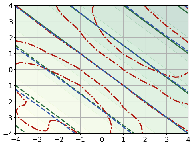
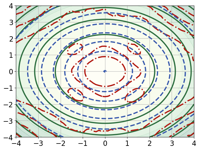
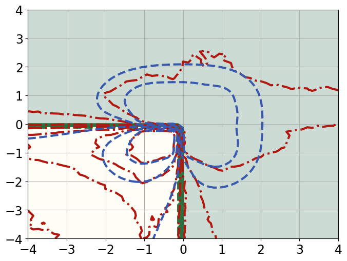
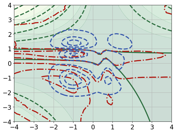
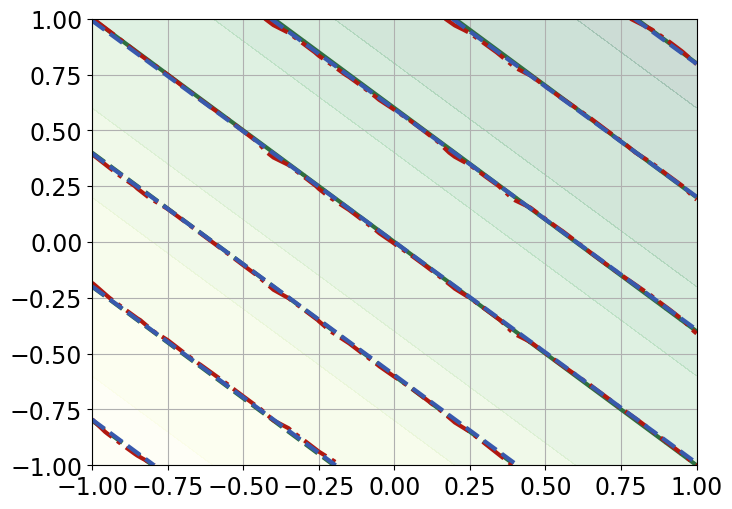
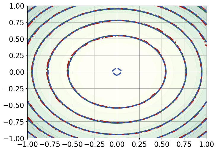
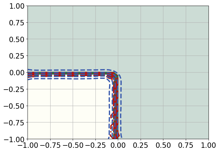
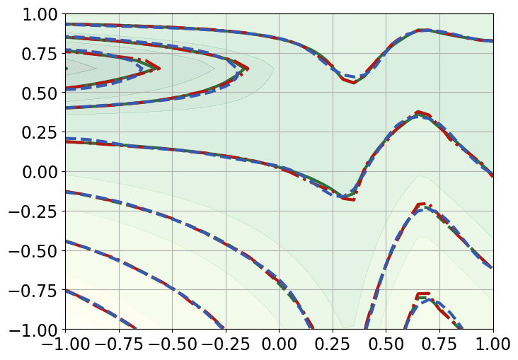
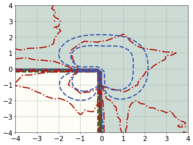
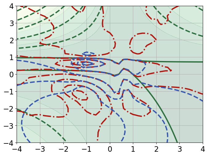
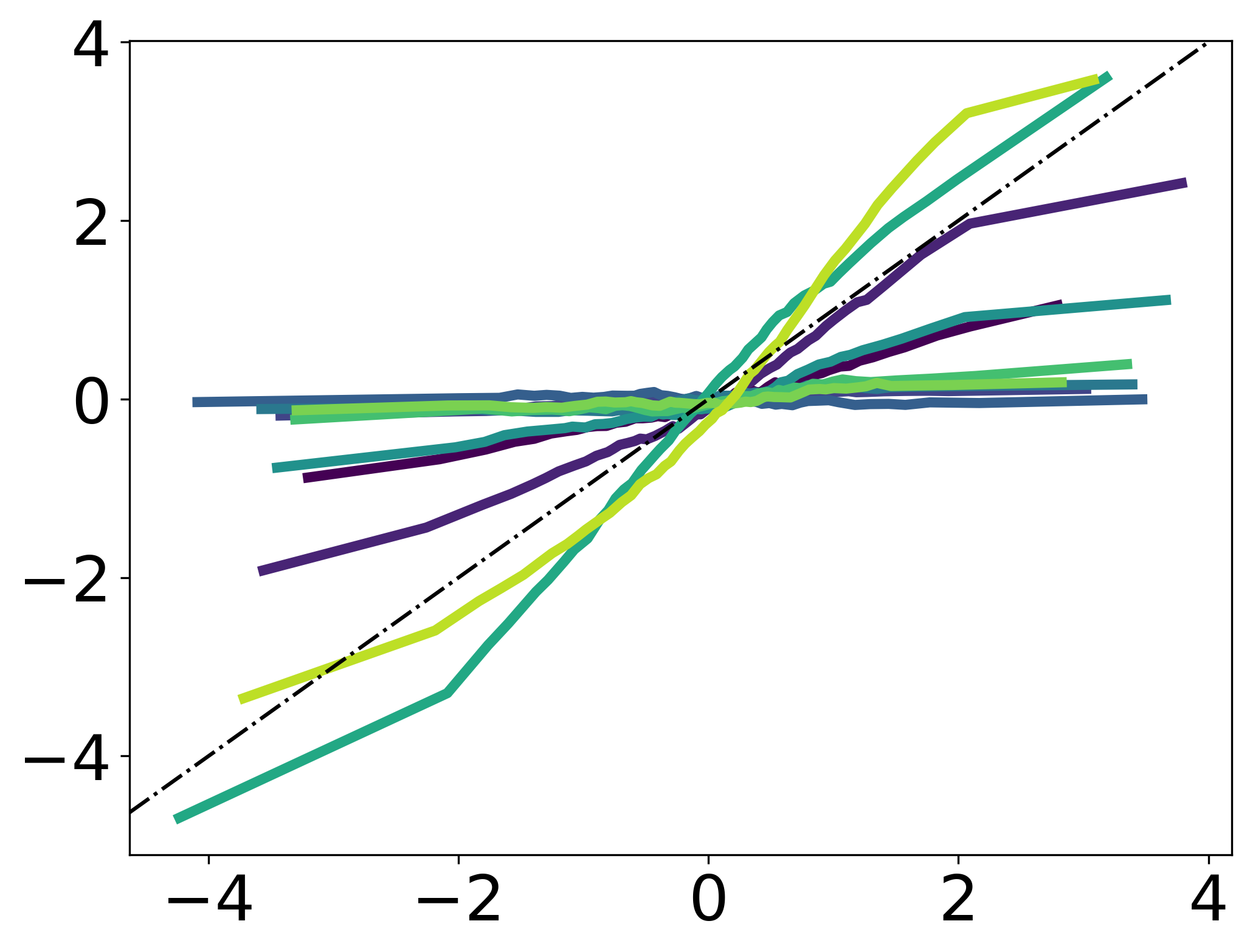
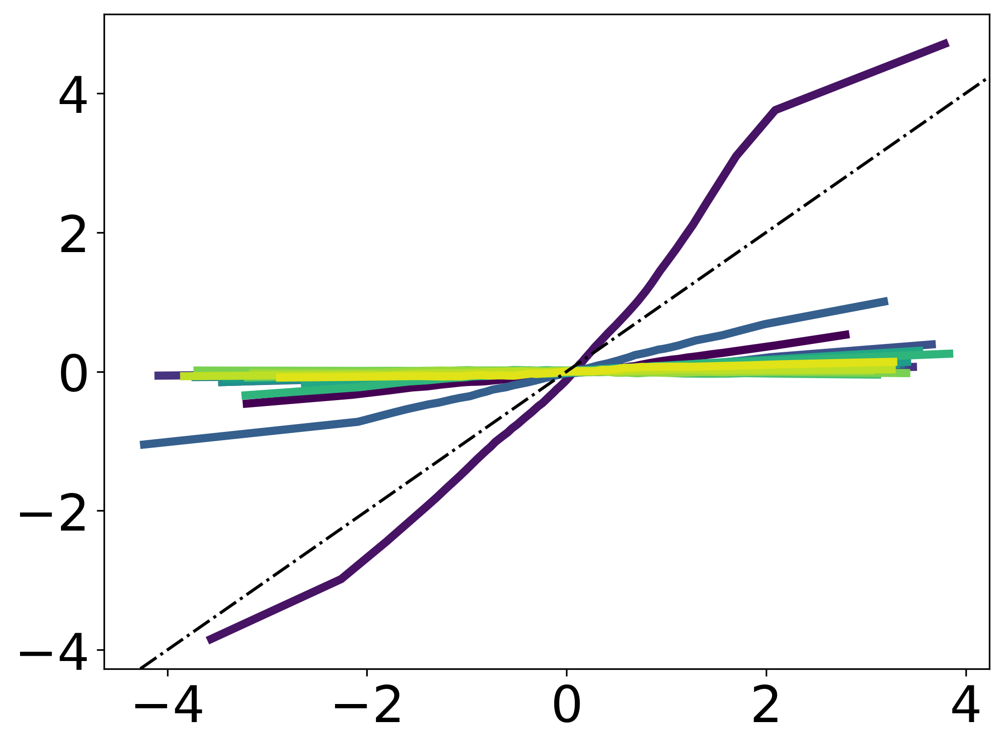
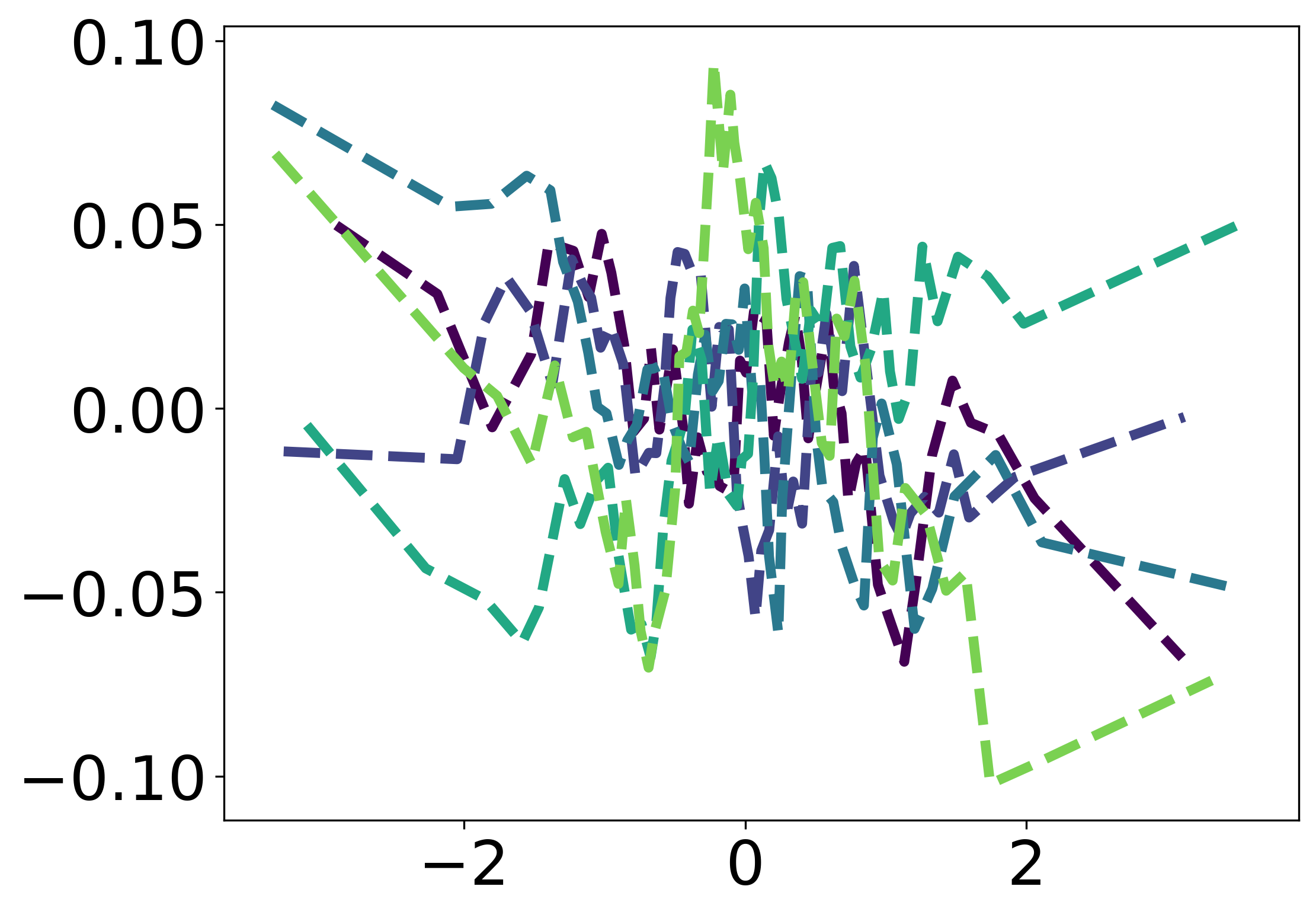
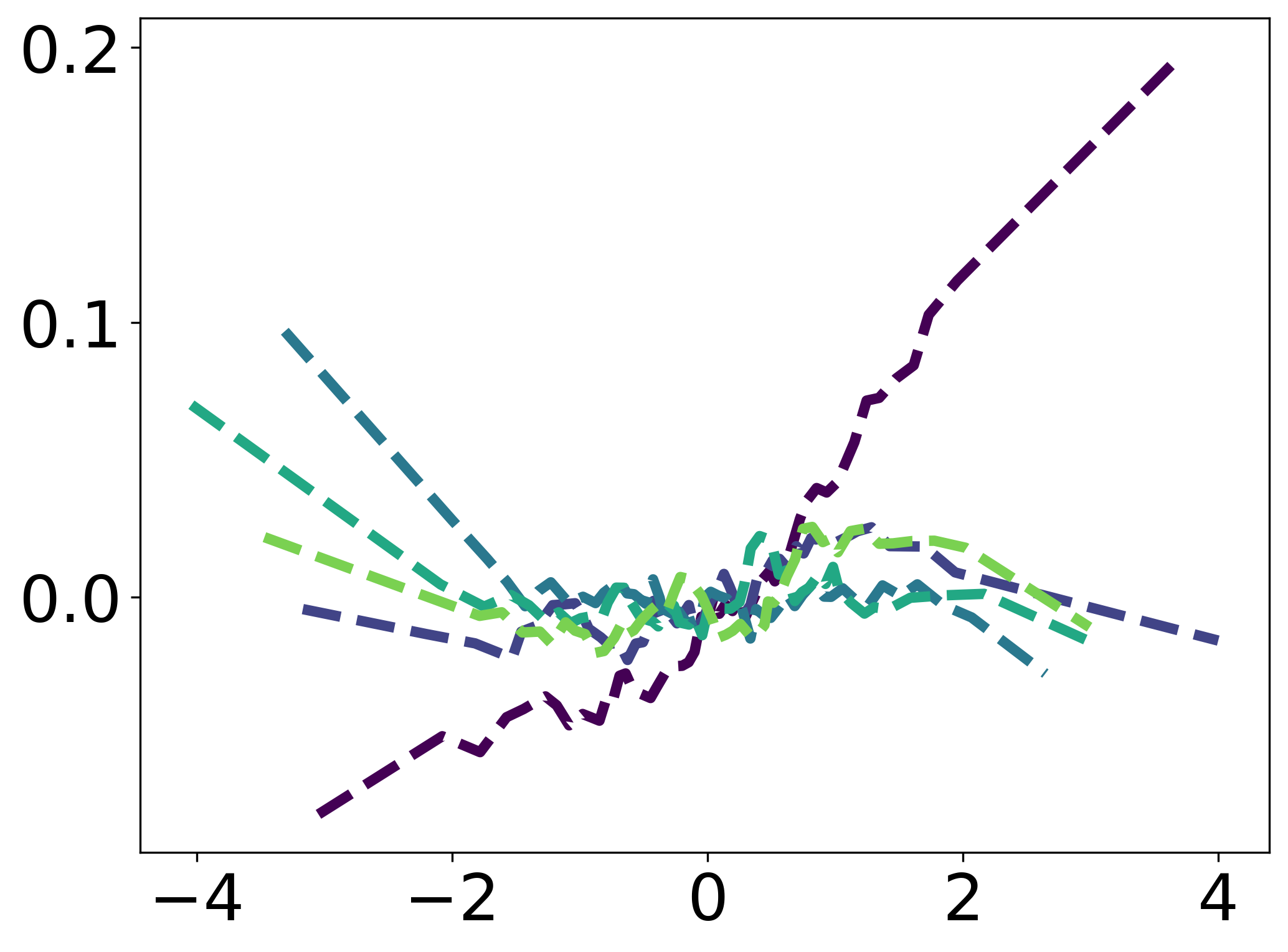
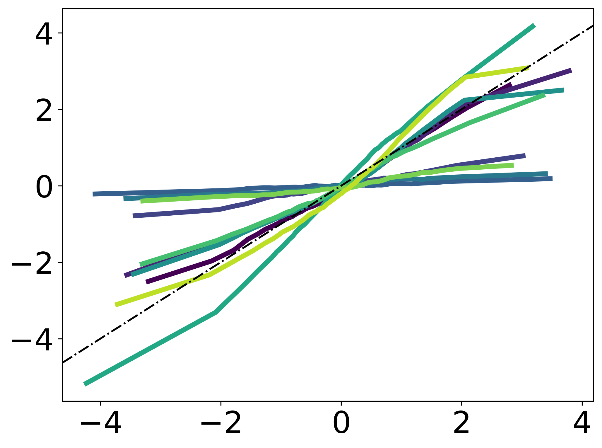
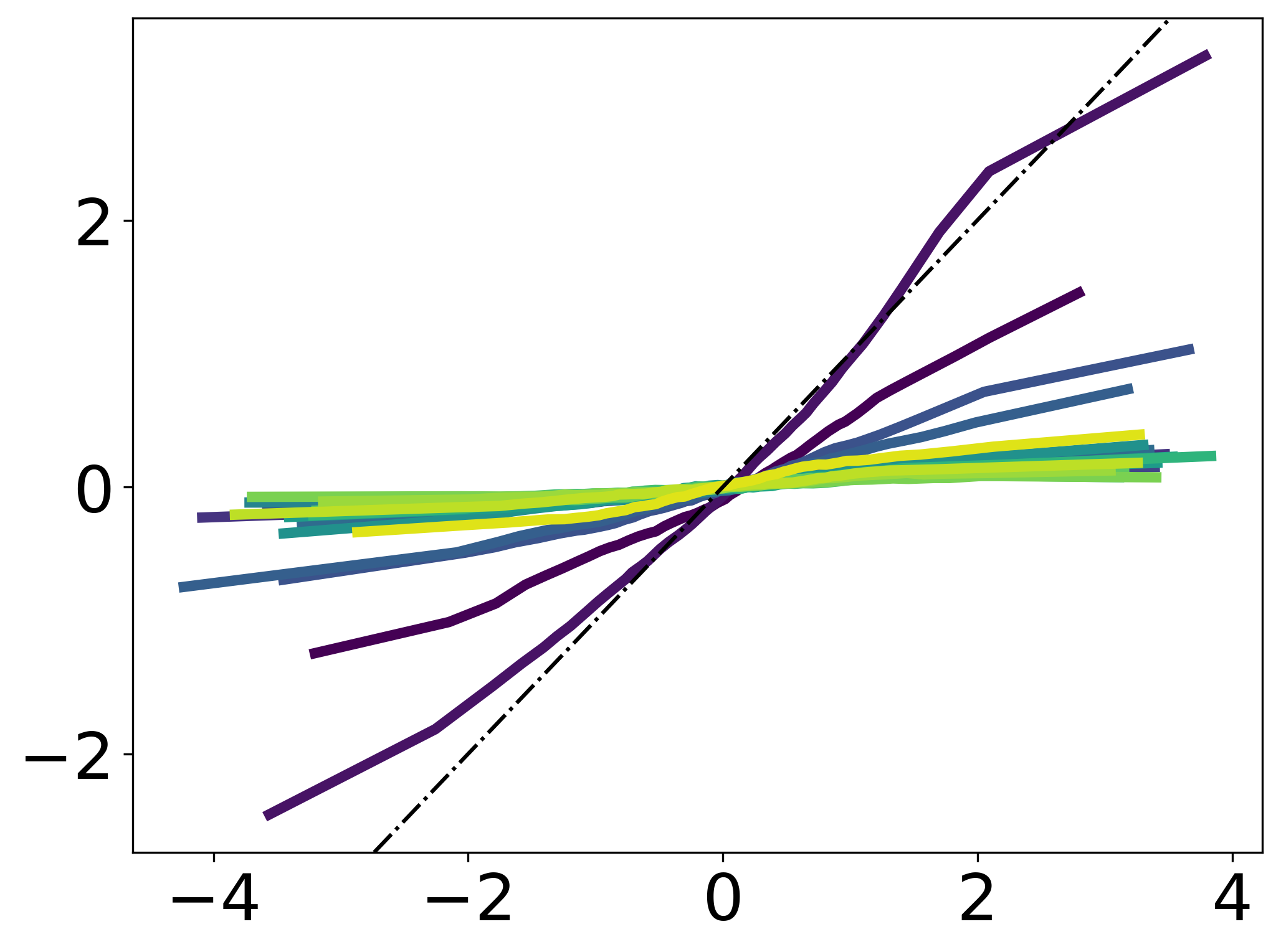
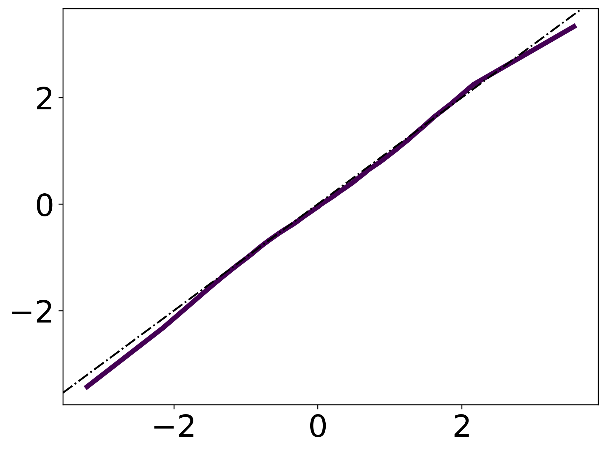
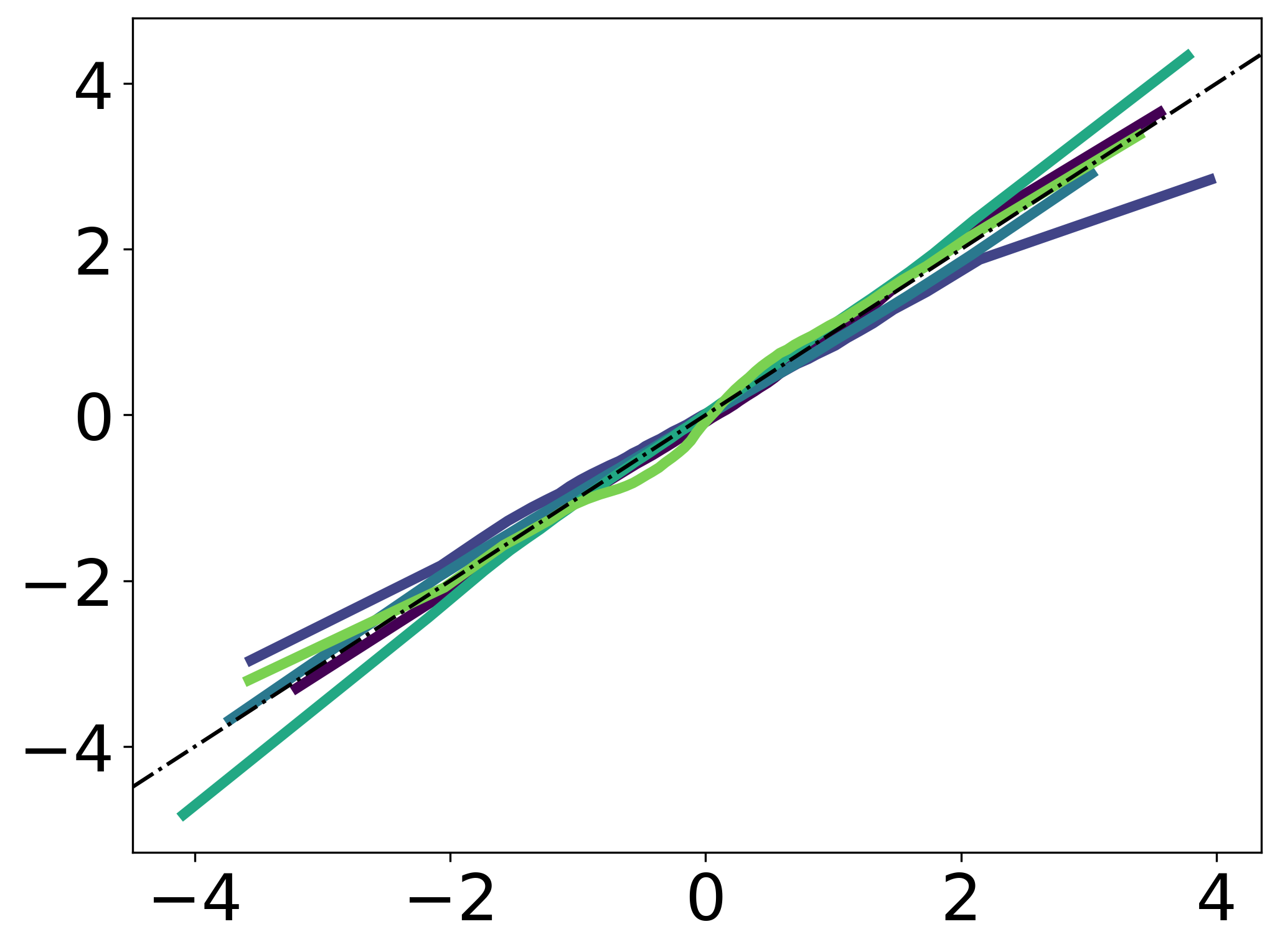
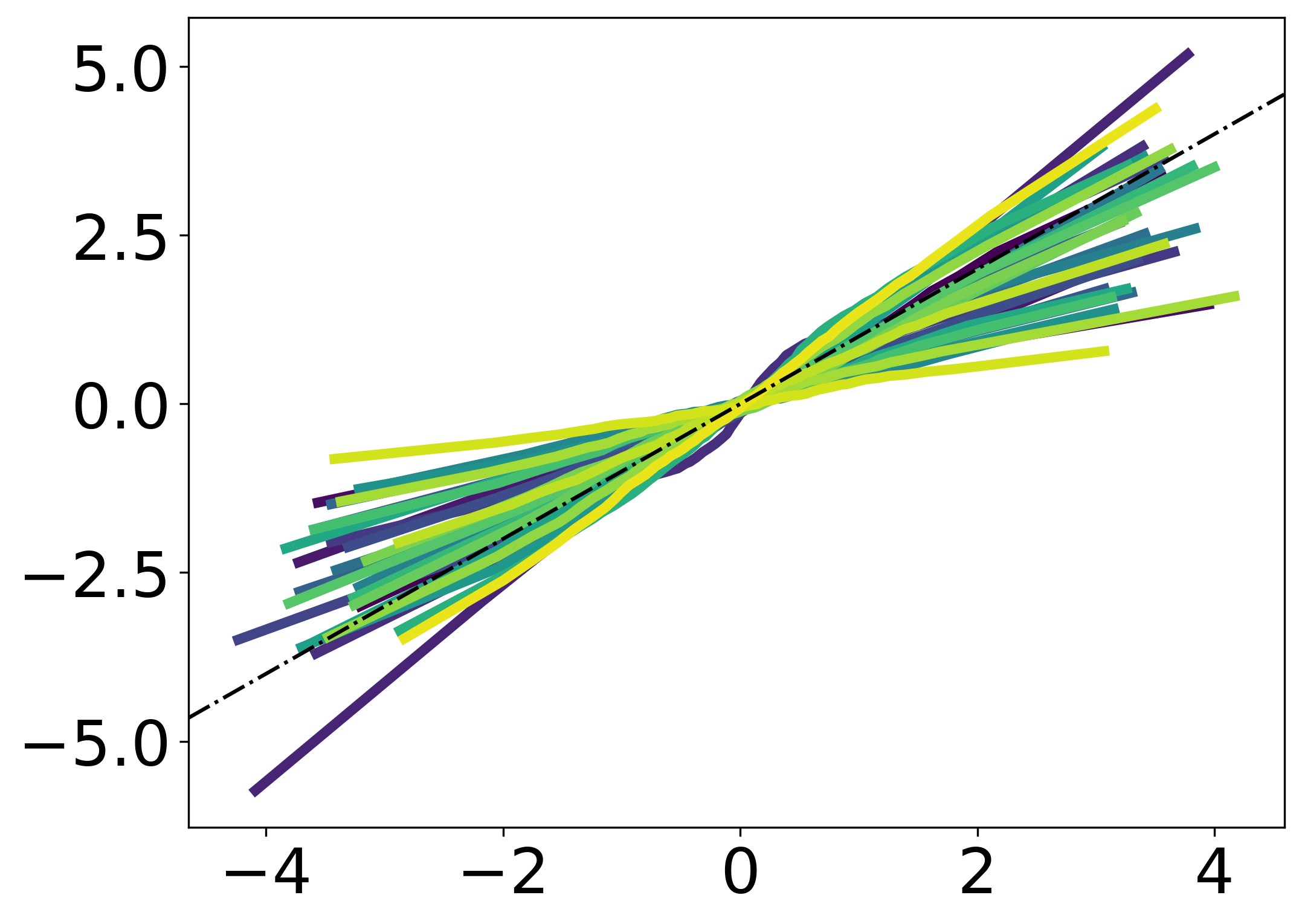
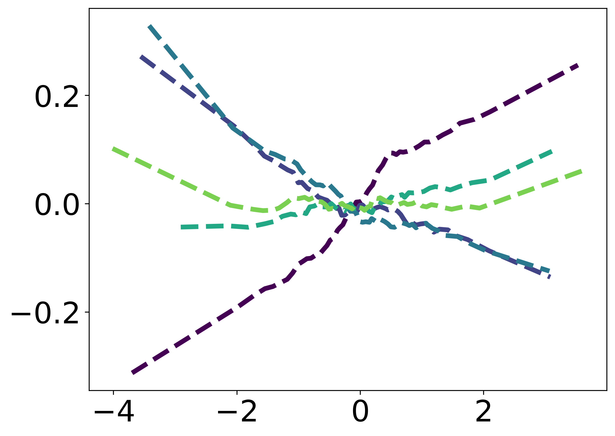
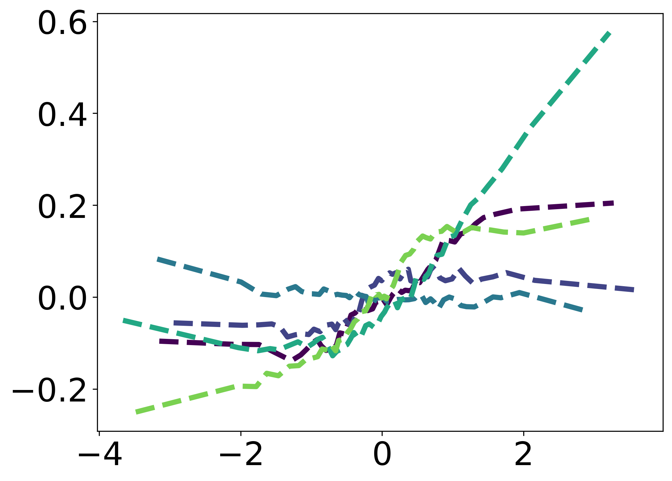
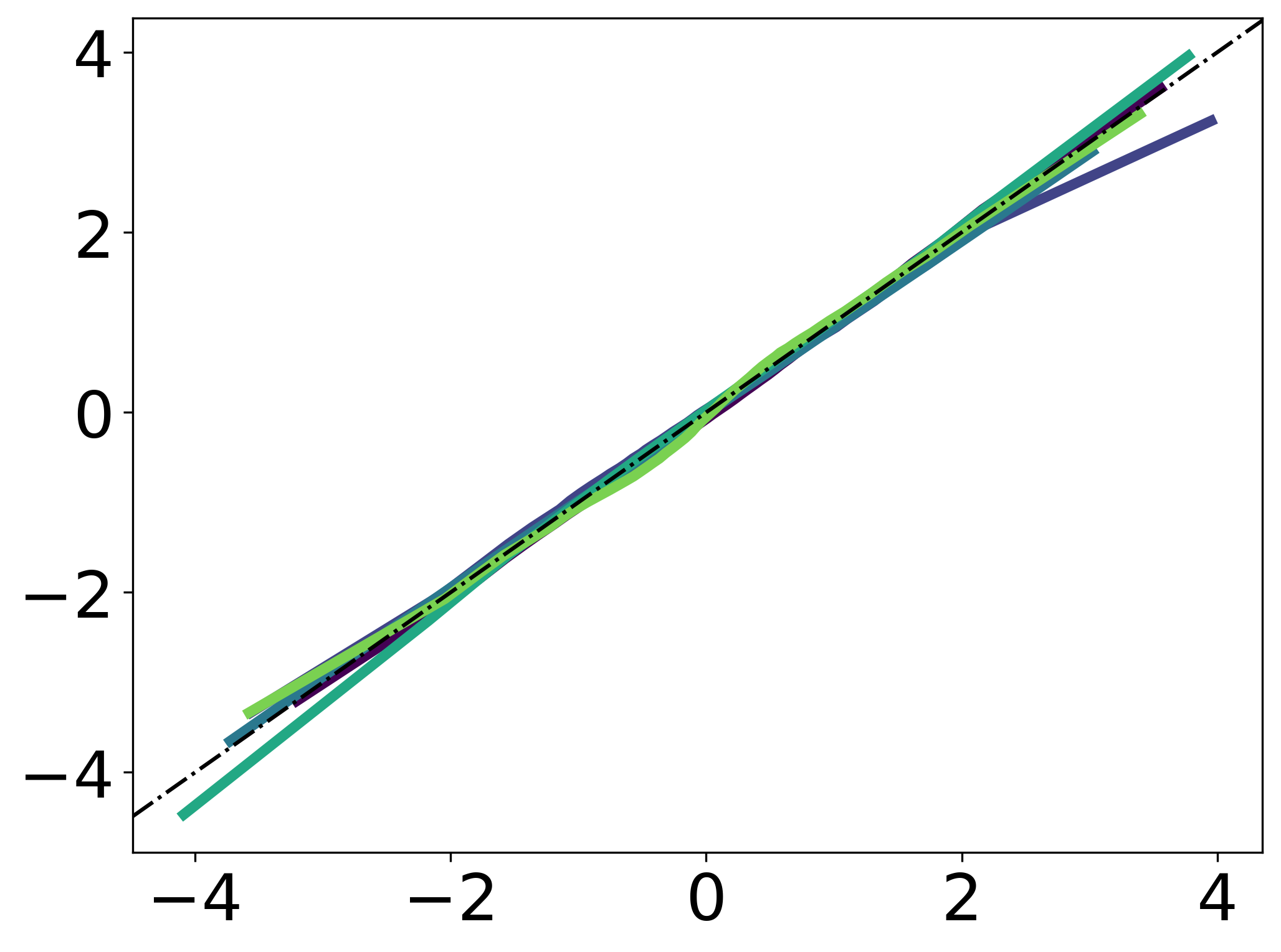
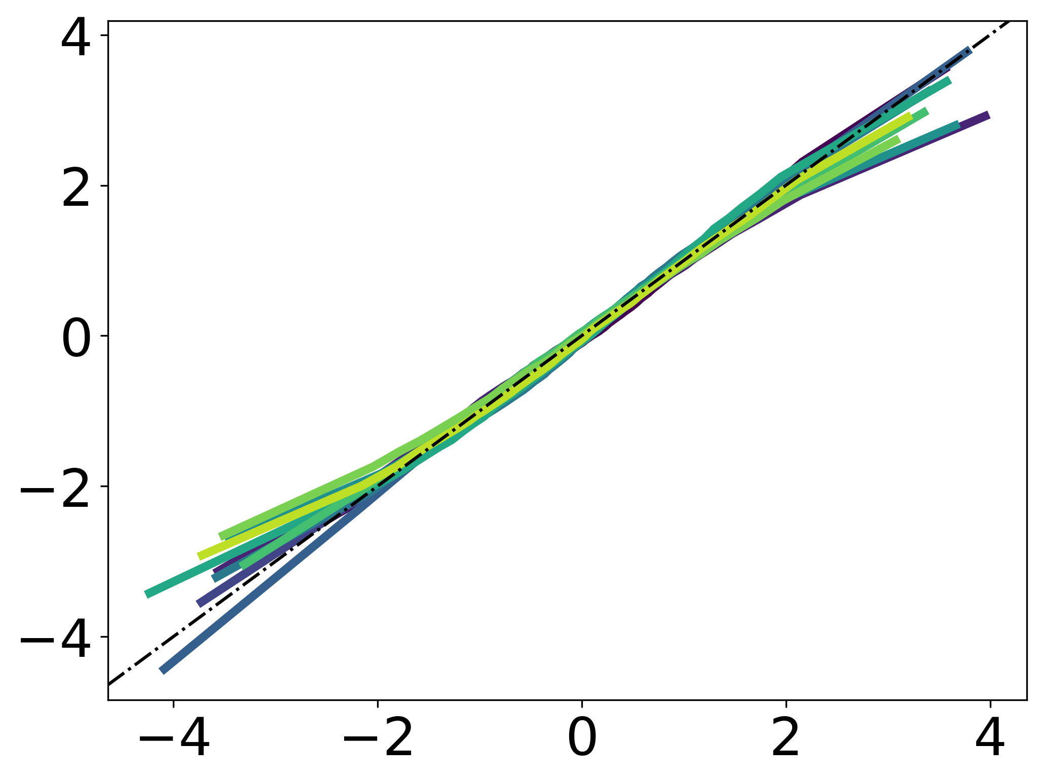
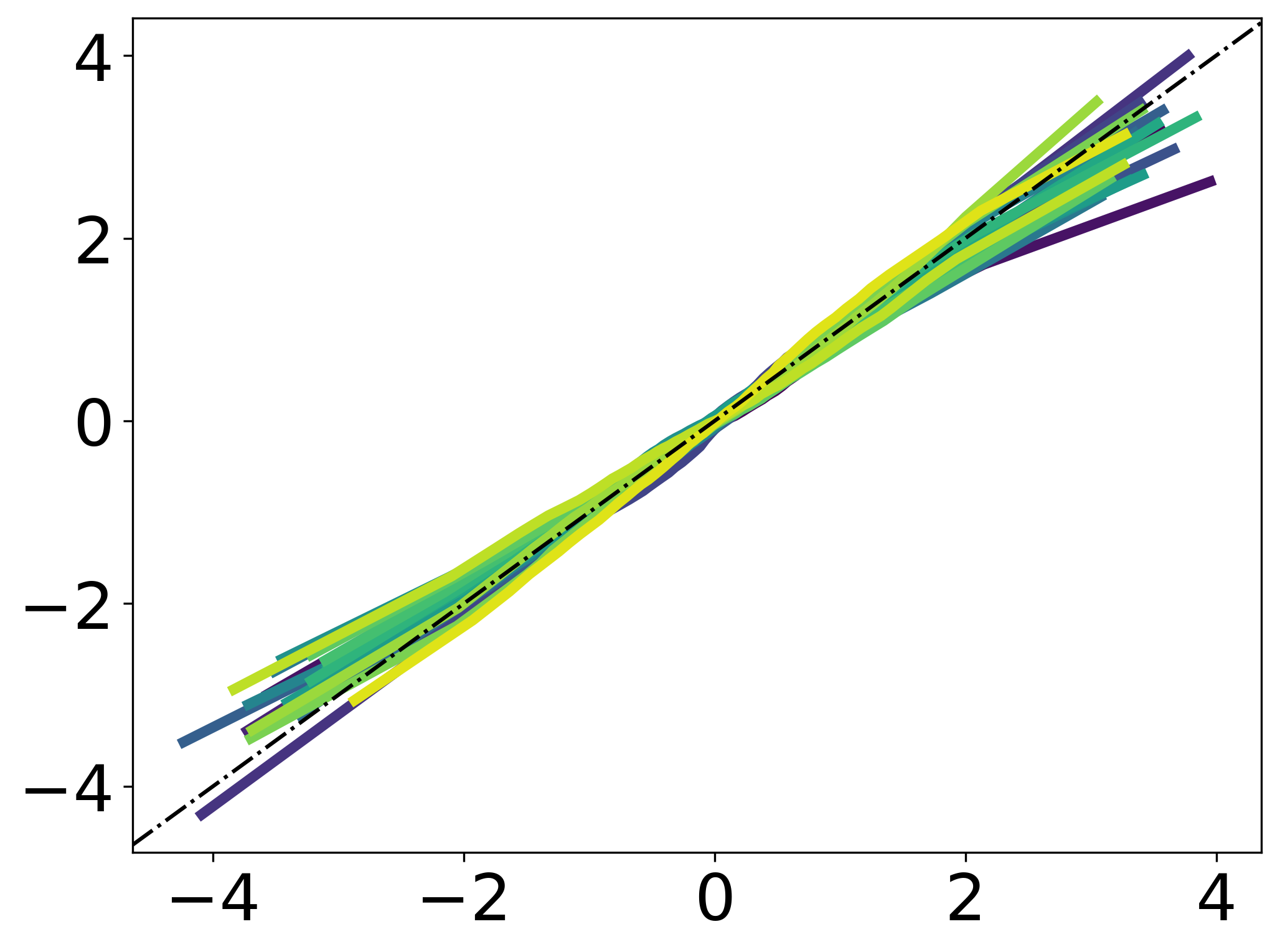
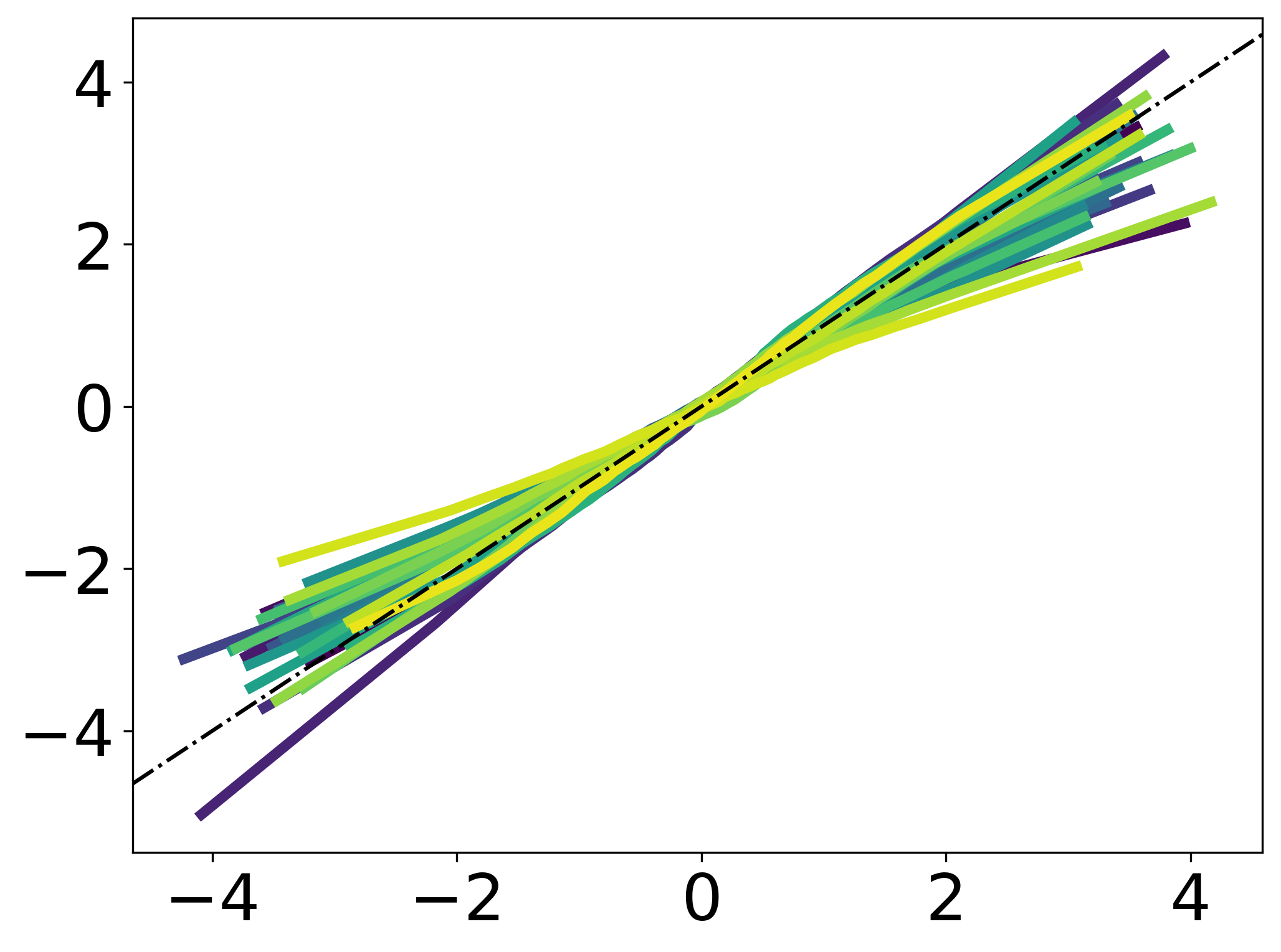
In our first experiment, we examine how TabPFN interpolates and extrapolates from observed data. For simplicity, we demonstrate this in a univariate setting and with respect to four simple functional forms: (i) a linear function, (ii) a quadratic function, (iii) a step function, and (iv) a piecewise linear function. The results for training data points are shown in Figure 4, with the results for and experimental details deferred to Appendix D. For comparison, we also show the results obtained using Gaussian process regression (GPR) with both kernel and noise variance parameters tuned using marginal likelihood. We observe that in all cases, TabPFN fits a smoothly-varying curve that broadly resembles the GPR curve within the interpolation region. The notable differences are:
-
•
Unlike GPR, TabPFN seems not to suffer from the Gibbs phenomenon (fluctuations at the point of discontinuity of a step function).
-
•
TabPFN extrapolates at roughly the same level of the last observed response, whereas GPR quickly asymptotes to zero (the GPR prior mean).
-
•
TabPFN is more conservative than GPR at fitting a quickly-varying function. GPR is able to roughly approximate the piecewise-linear function with , whereas TabPFN still outputs a constant model.
-
•
TabPFN has a more diffuse conditional predictive distribution compared to GPR, especially away from the interpolation region.
4.2 Comparison with LASSO regression
In our second experiment, we perform a head-to-head comparison between TabPFN and LASSO when applied to sparse linear regression. The main point is to demonstrate that while TabPFN is seemingly flexible enough to adapt to any type of functional structure, it can nevertheless sometimes recognize and adapt to situations when the dataset contains additional parametric structure, even competing favorably with methods designed specifically to handle that structure. In addition to this, we also observe some other unexpected results.
4.2.1 Experimental design.
We broadly follow the experimental design of Hastie, Tibshirani and Tibshirani [18]. We generate , with having sparsity (i.e., entries are and the rest are ). We consider two types of :
-
•
Beta-type I: has components equal to , spaced approximately evenly across the indices, and the rest equal to ;
-
•
Beta-type II: has its first components equal to , and the rest equal to .
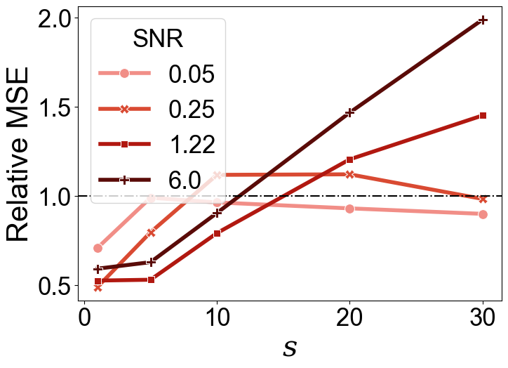
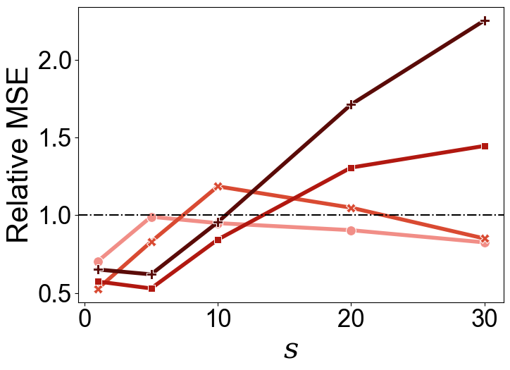
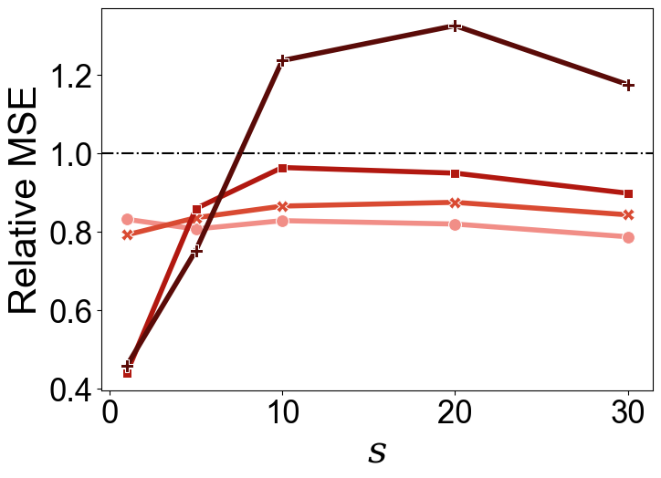
Features corresponding to non-zero (zero) coefficients are termed relevant (irrelevant). We fix and vary . The features are drawn i.i.d. from , where denotes a -dimensional Gaussian and is either the identity matrix or a matrix with -th entry equal to (banded correlation). Since beta-type I and II are equivalent when is identity, this gives distinct experimental scenarios. The response is generated with additive Gaussian noise, who variance is chosen to meet the desired signal to noise ratio (SNR), denoted by . Specifically, we set . We consider SNR values , spanning low to high noise regimes. Finally, we select . This yields experimental settings. For each setting, we evaluate performance on an independent test set of size , with the results averaged over experimental replicates. The regularization parameter of LASSO is tuned using -fold cross validation.
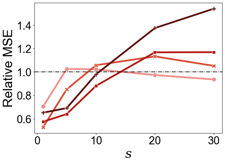
4.2.2 Prediction performance comparison.
In Figure 5, we plot the relative test MSE (averaged over repetitions) of TabPFN to that of LASSO across all experimental settings. We observe that TabPFN generally outperforms LASSO when either the SNR is low or sparsity level is high (i.e. small ). However, the performance of TabPFN can be much worse than LASSO for low sparsity (i.e. large ) settings, especially when SNR is high. Given that LASSO itself is not especially suited to dense linear regression, this also reveals that TabPFN has a severe inductive bias against dense linear structure.666In other unreported experiments, we also observed that TabPFN performs poorly more generally whenever the regression function depends on a relatively large number of features.
4.2.3 How linear is the TabPFN model?
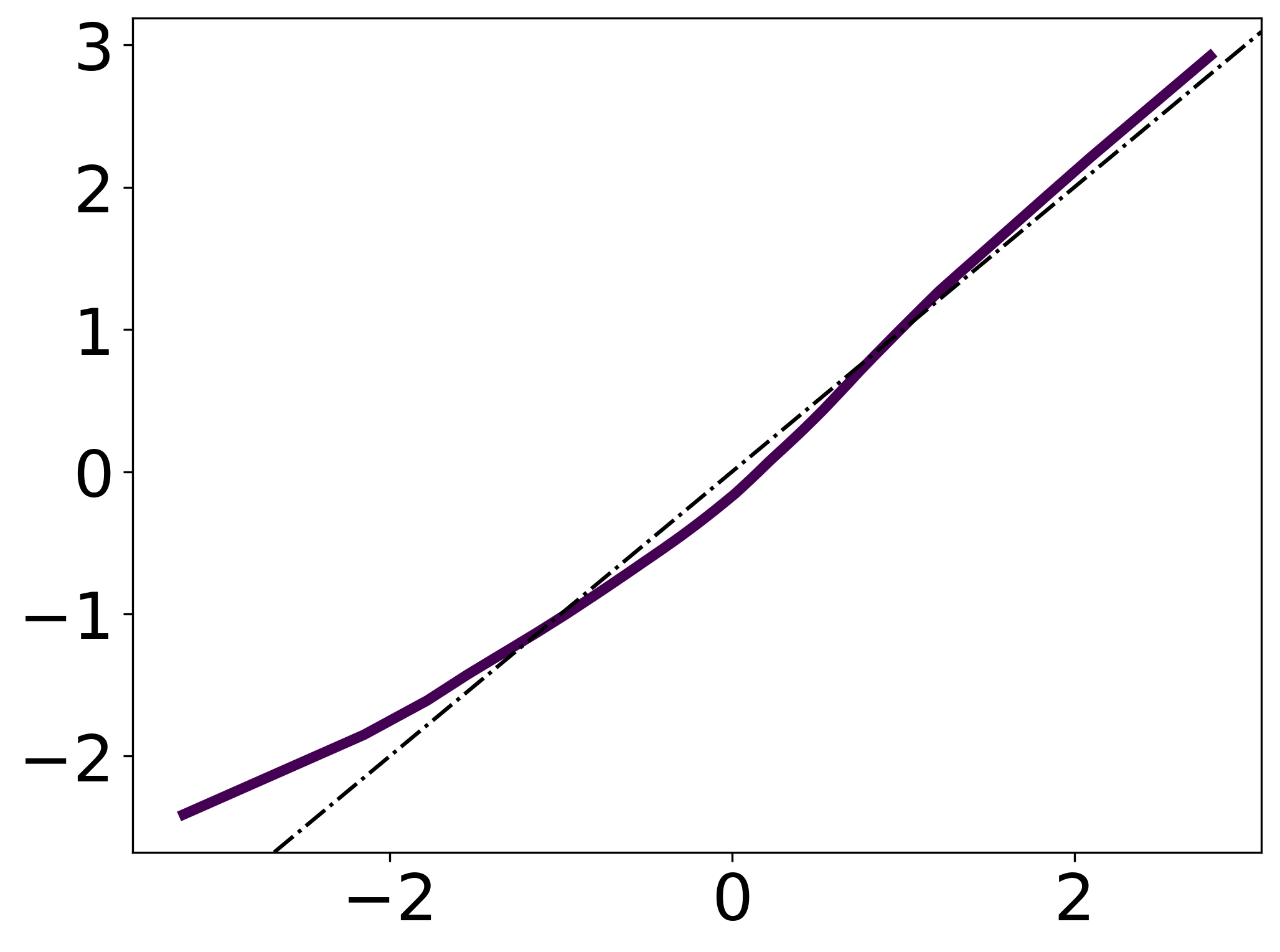
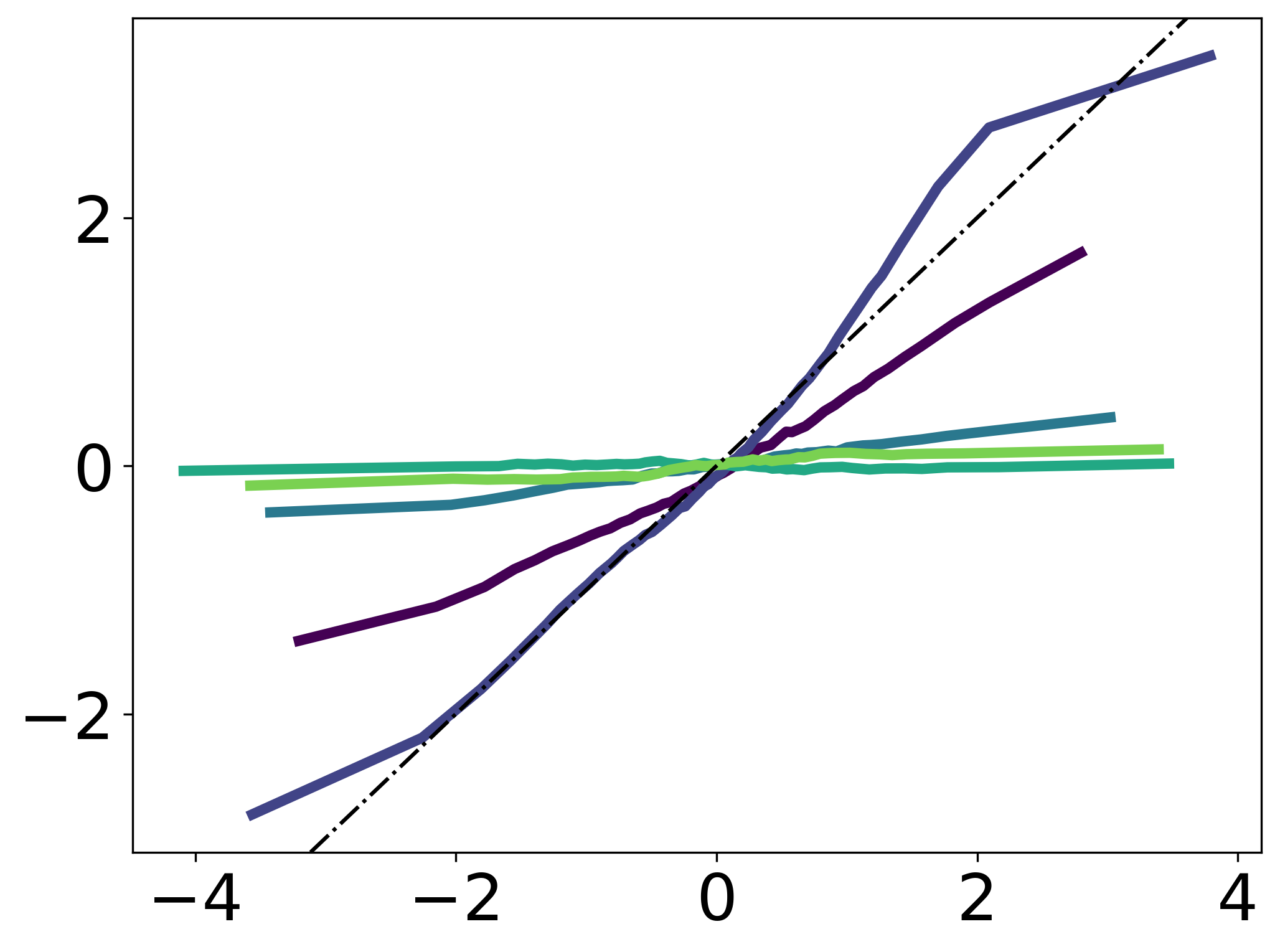
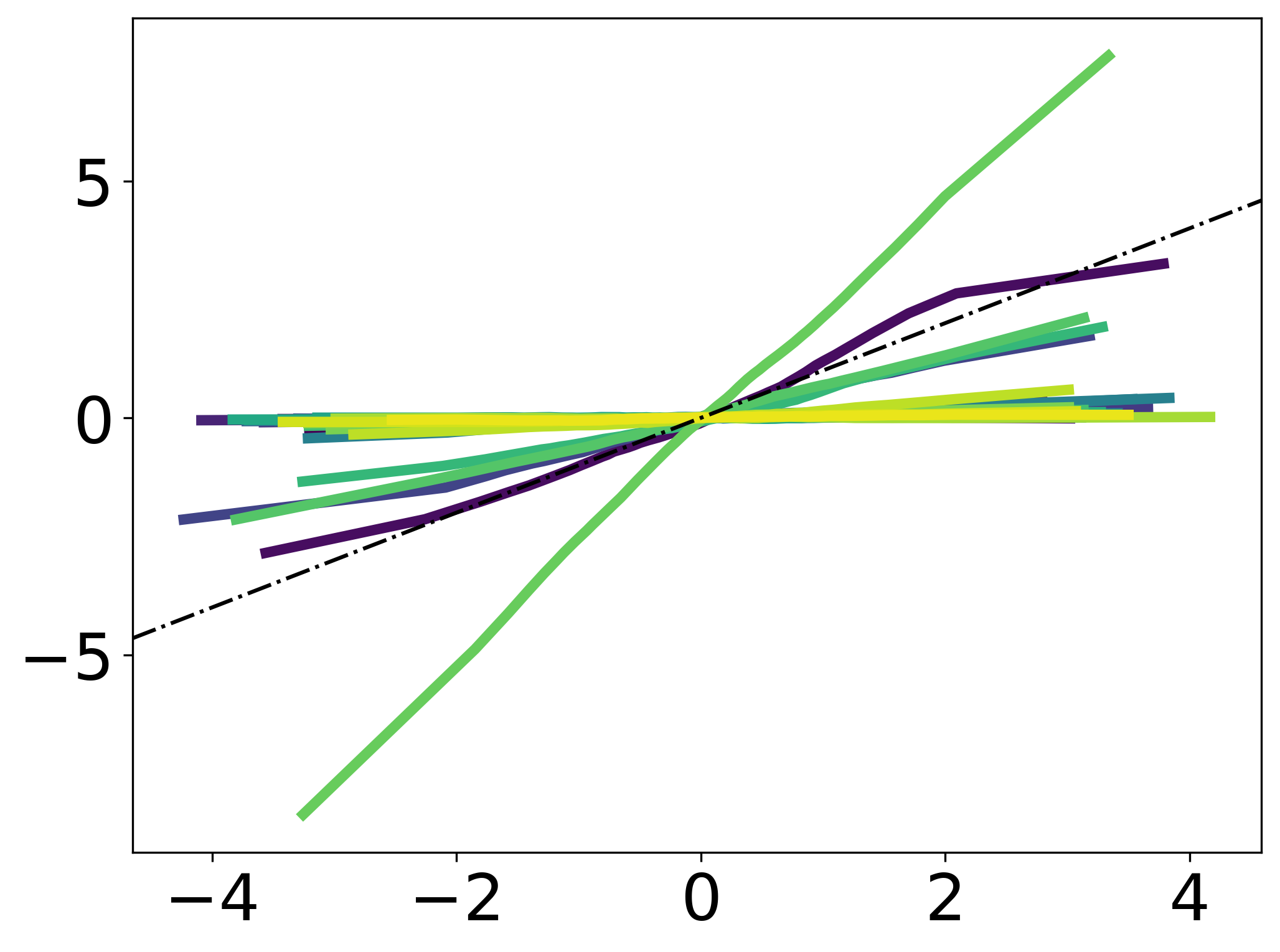
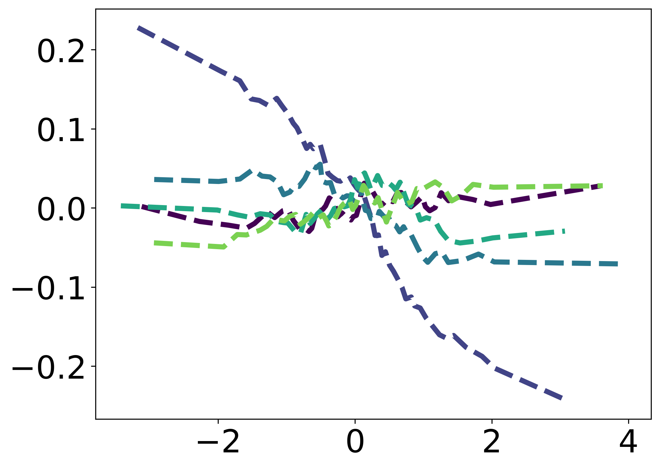
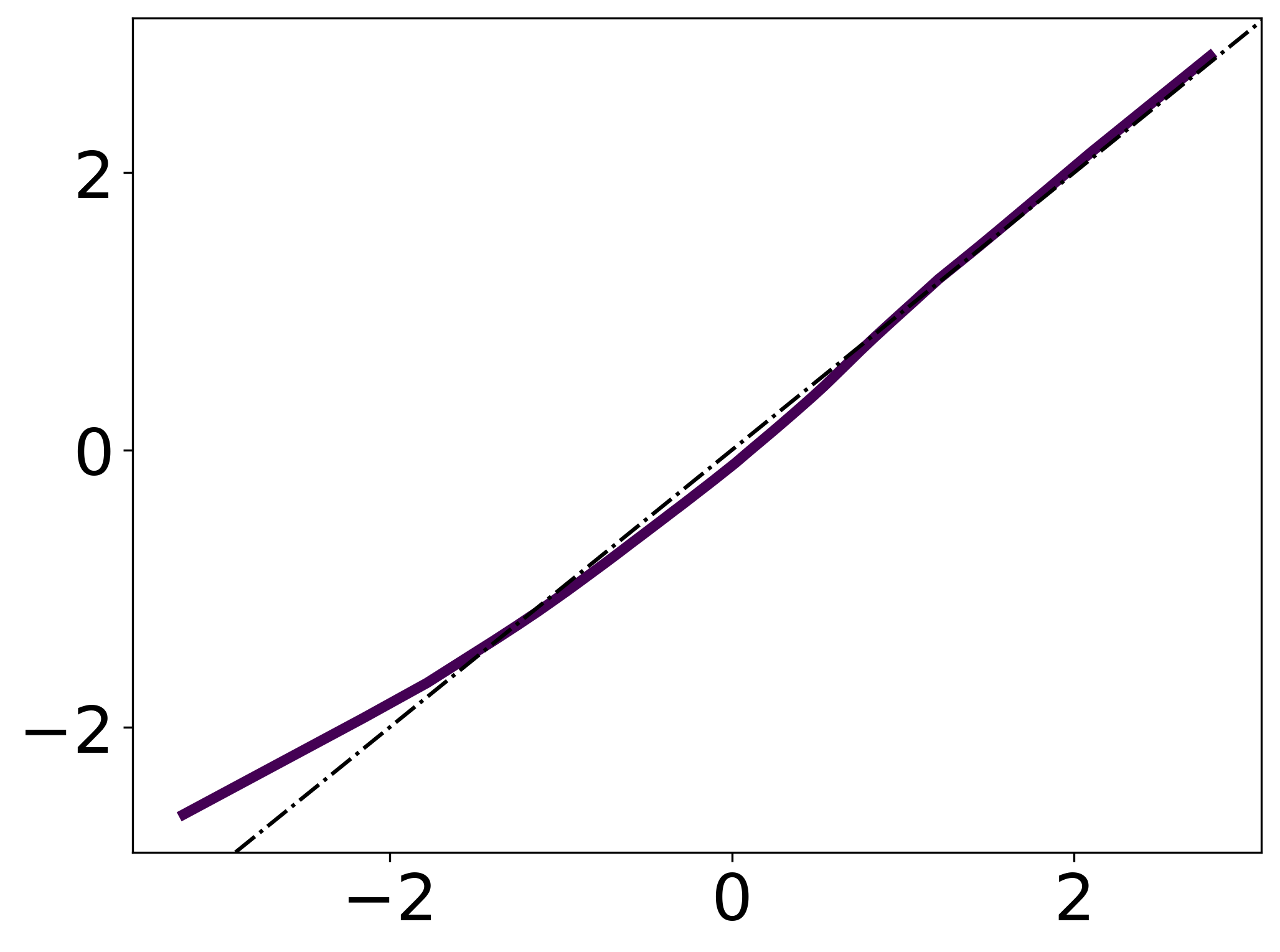
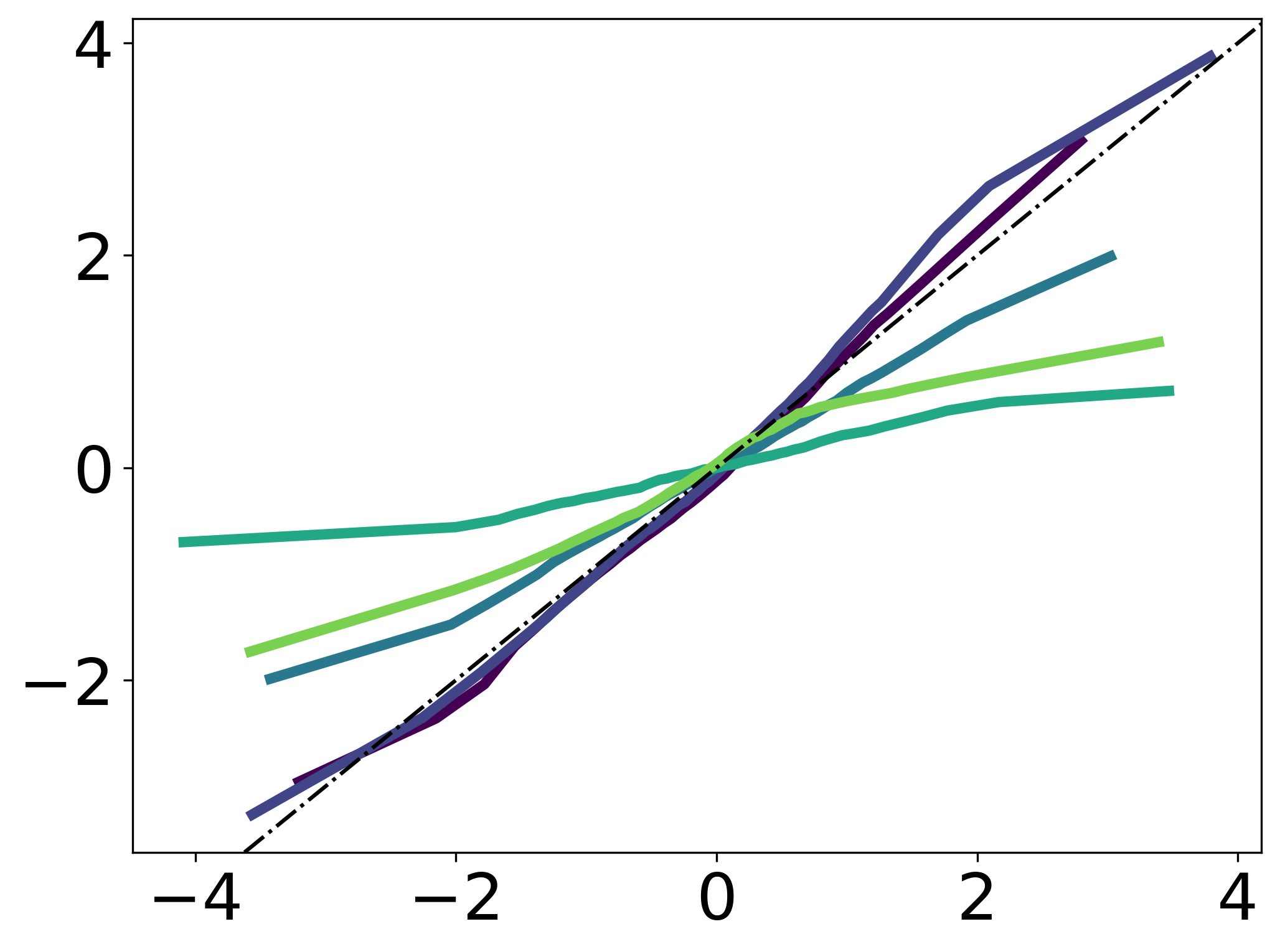
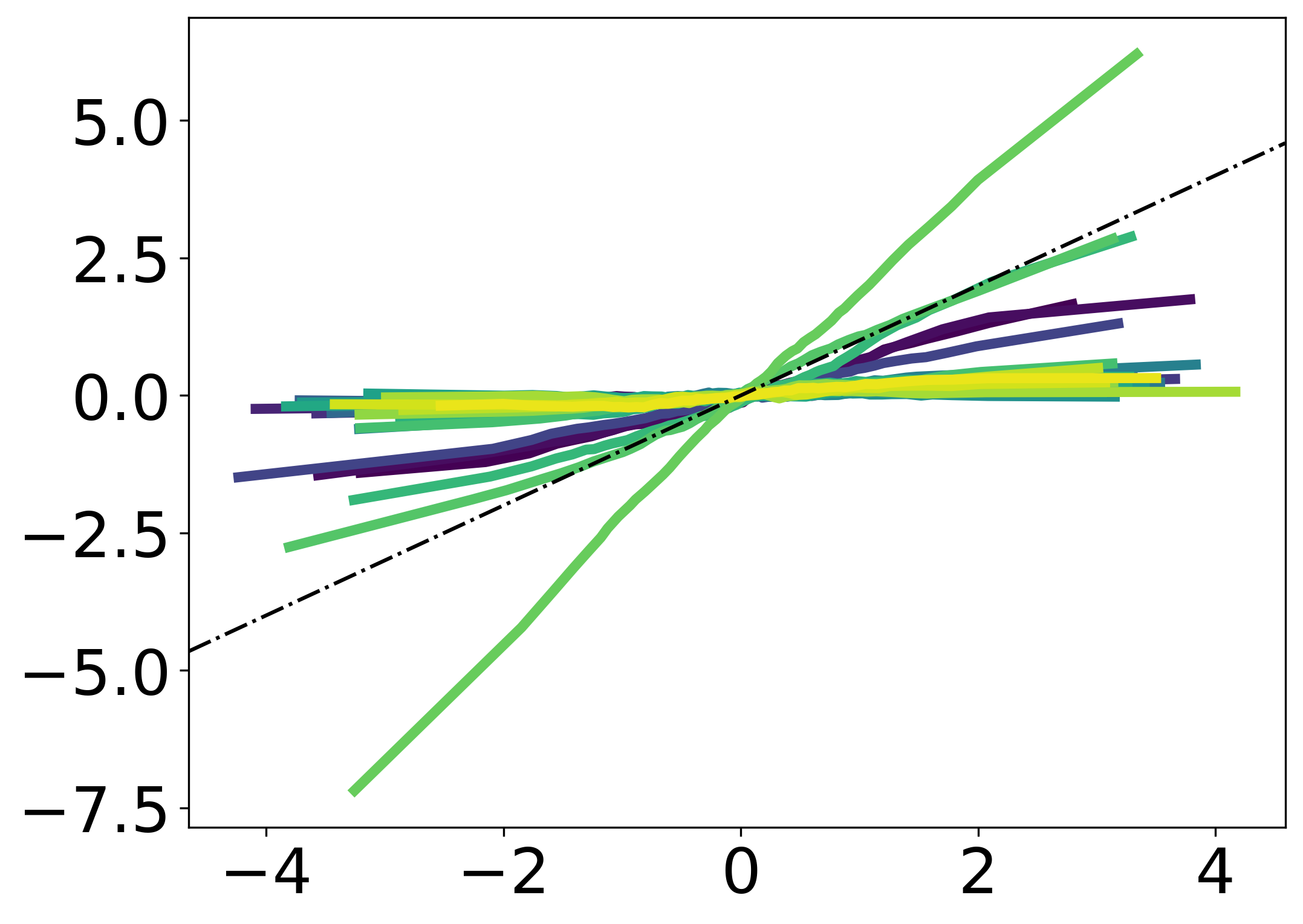
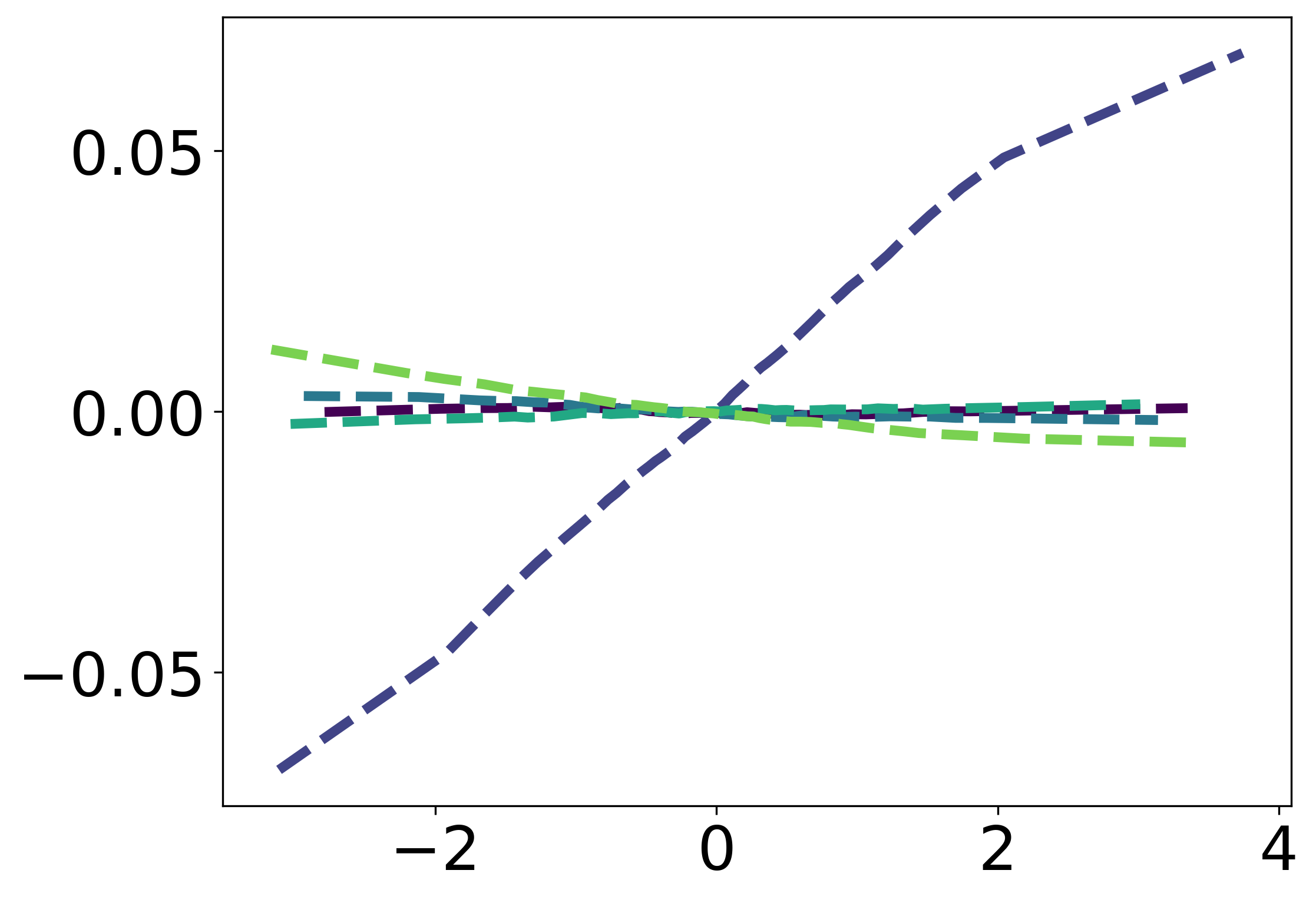
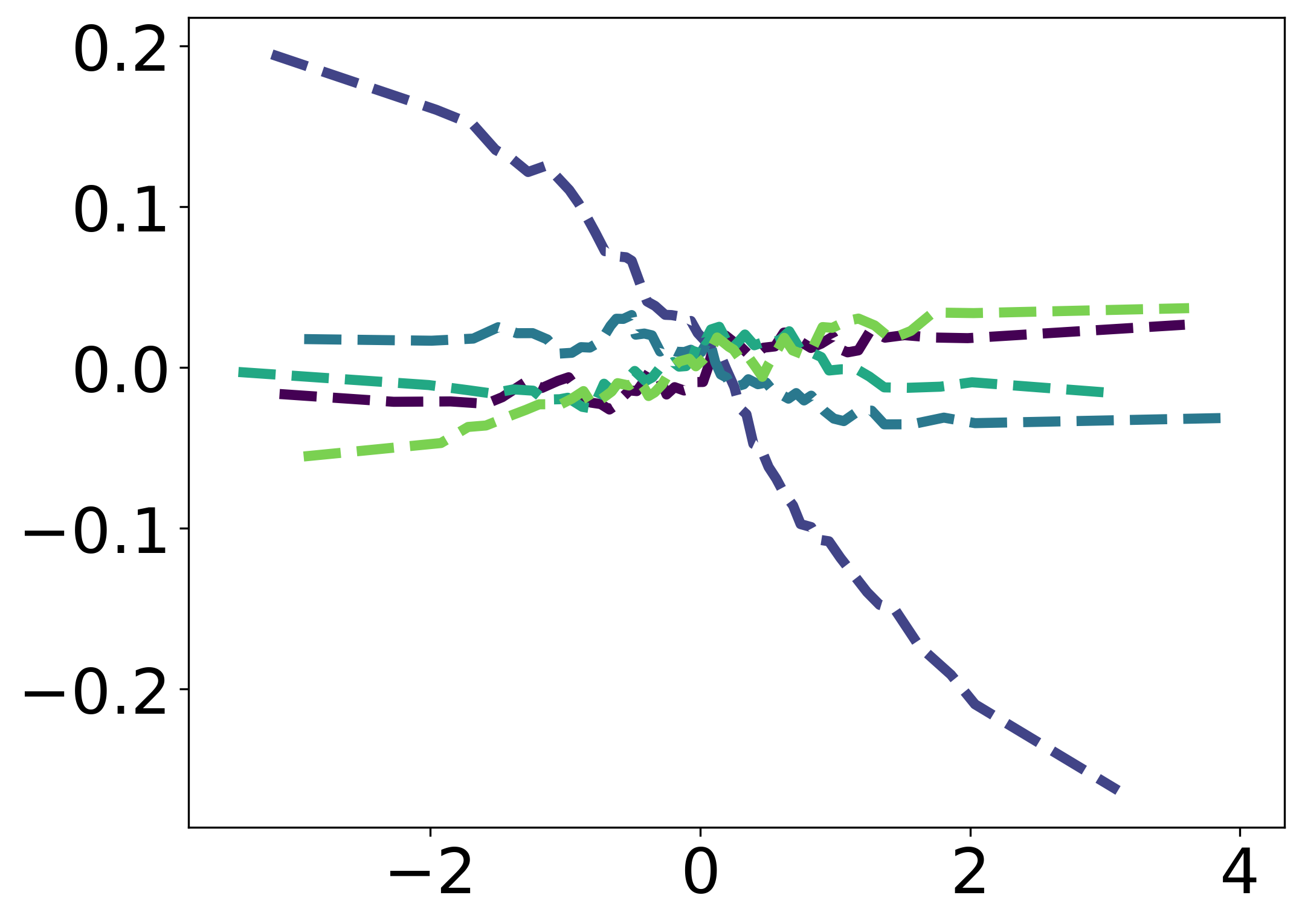
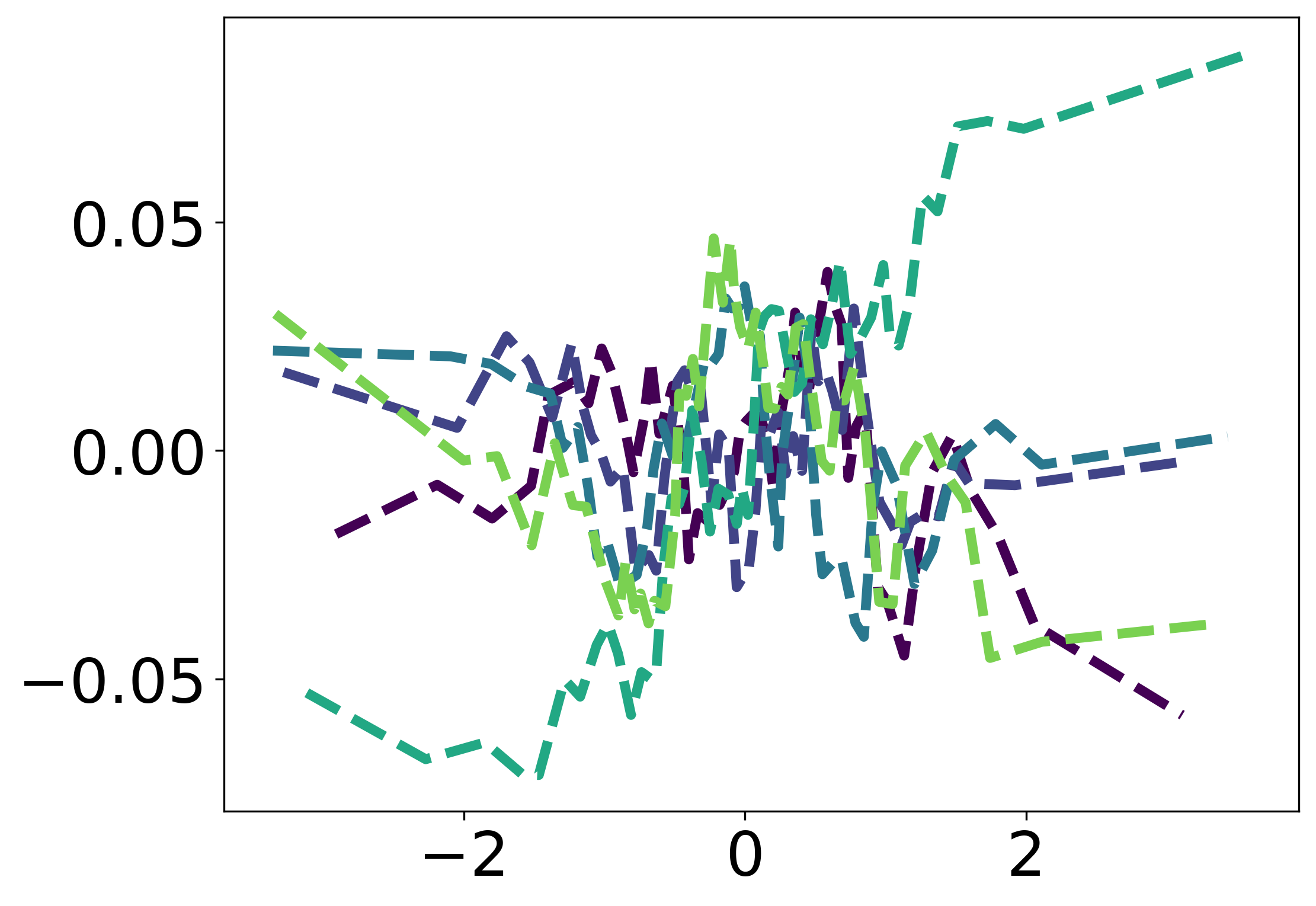
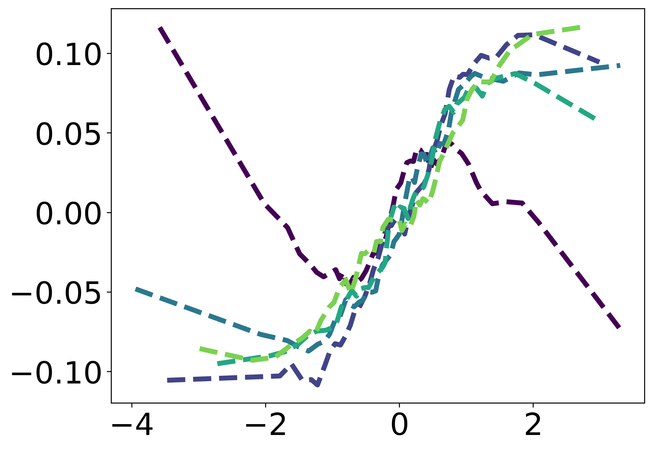
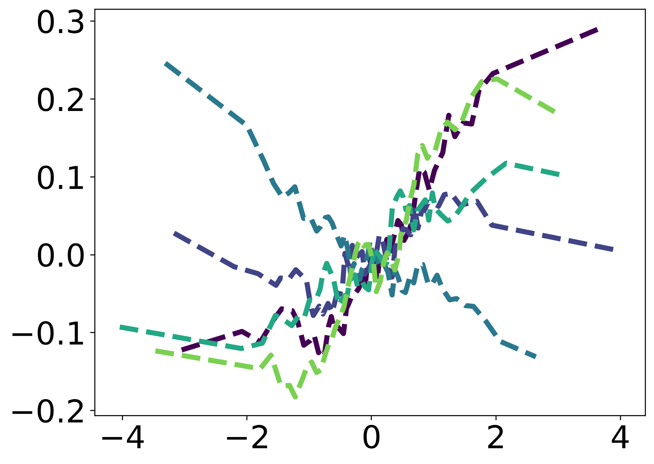
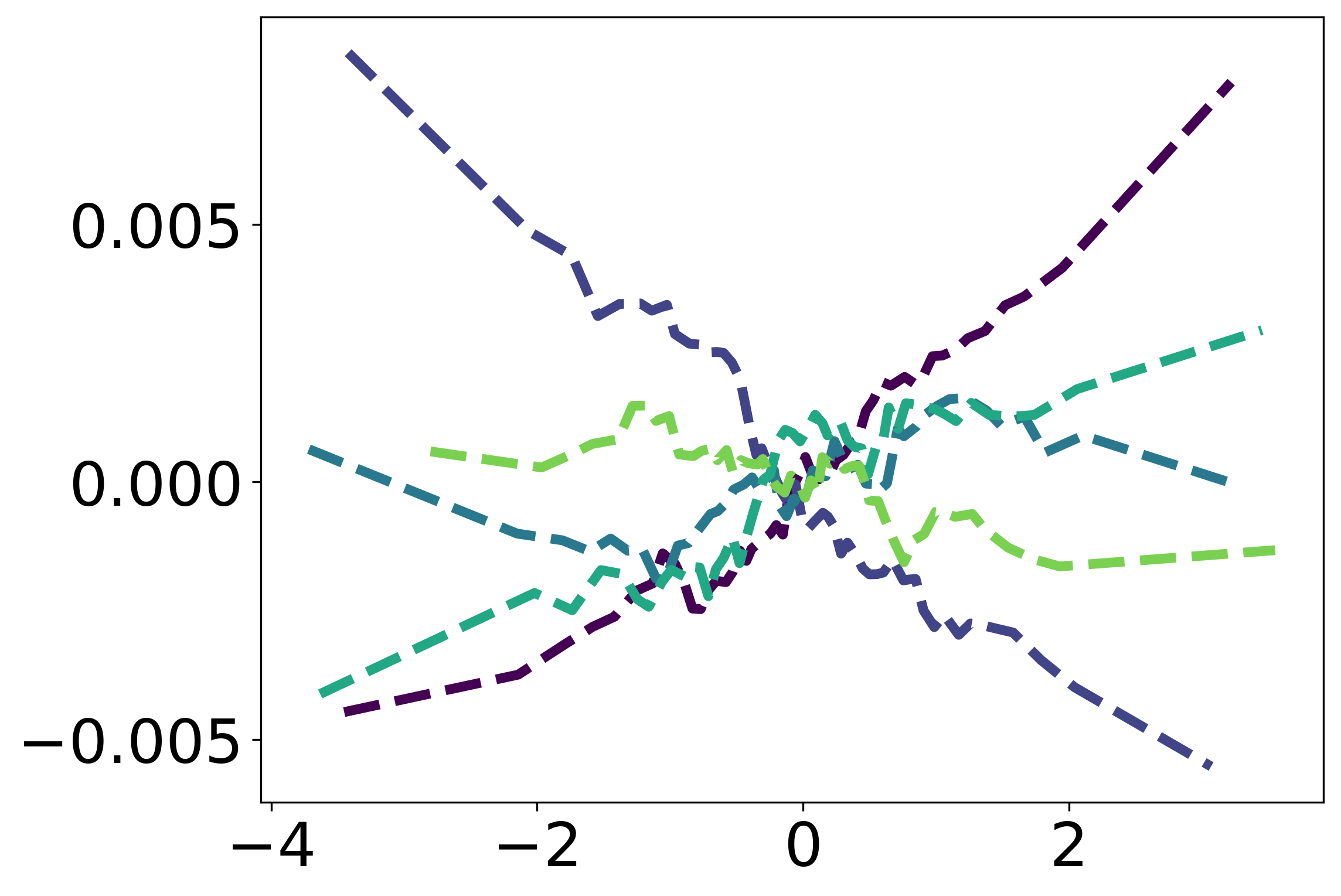
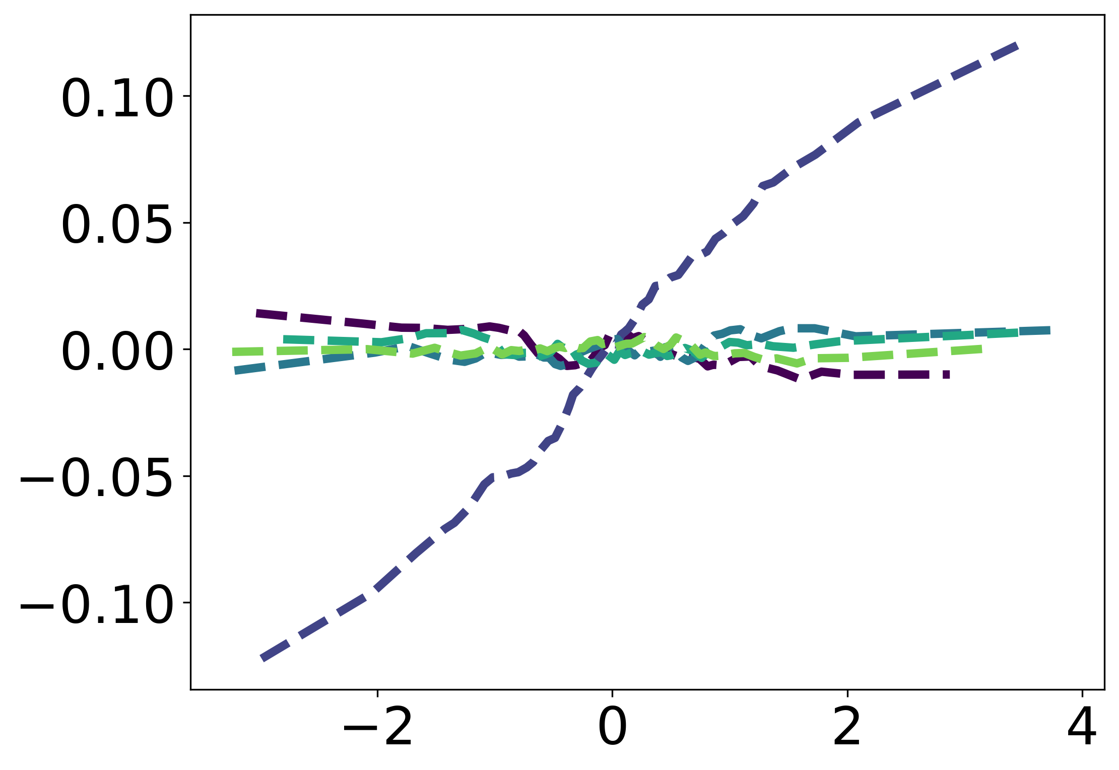
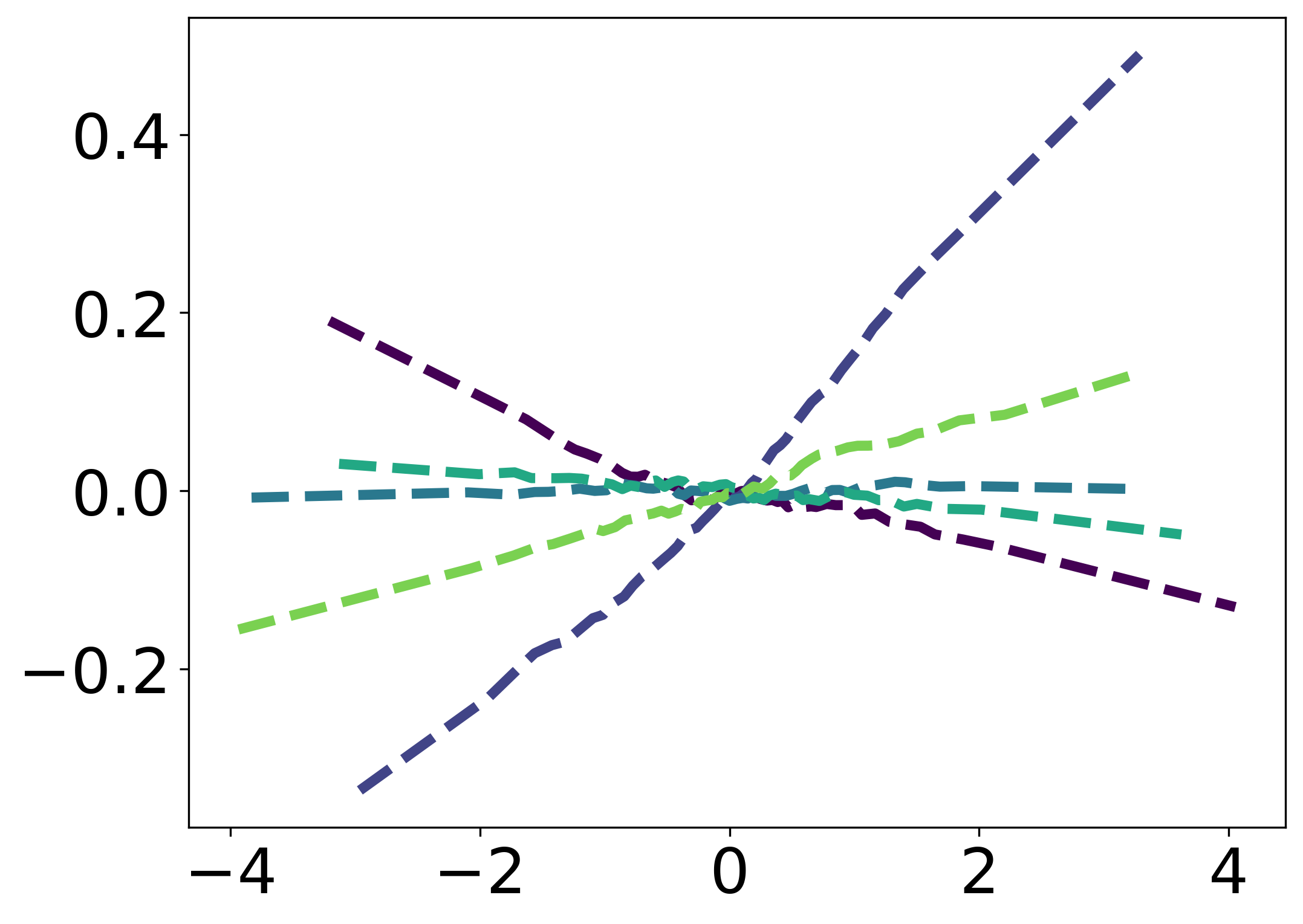
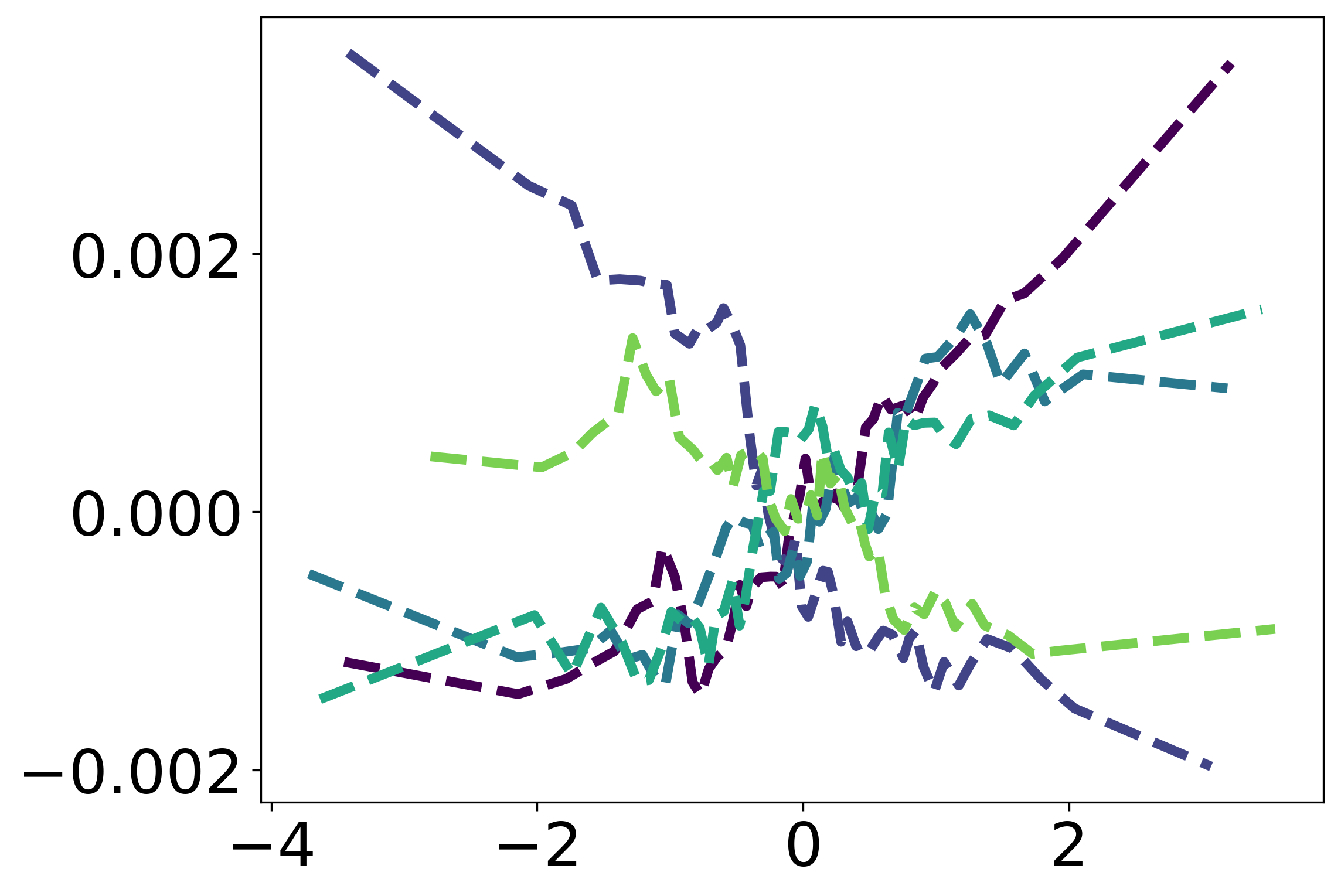
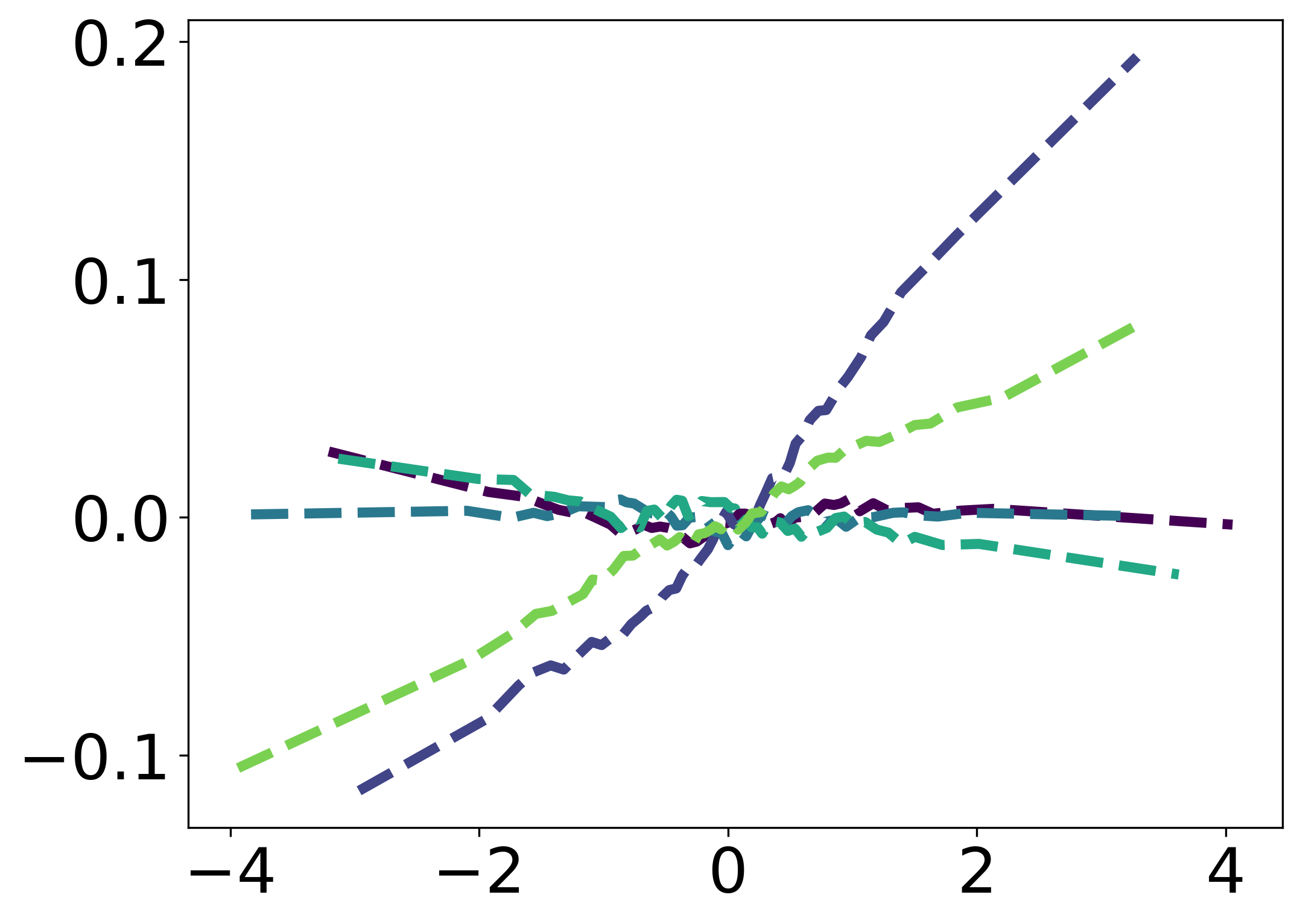
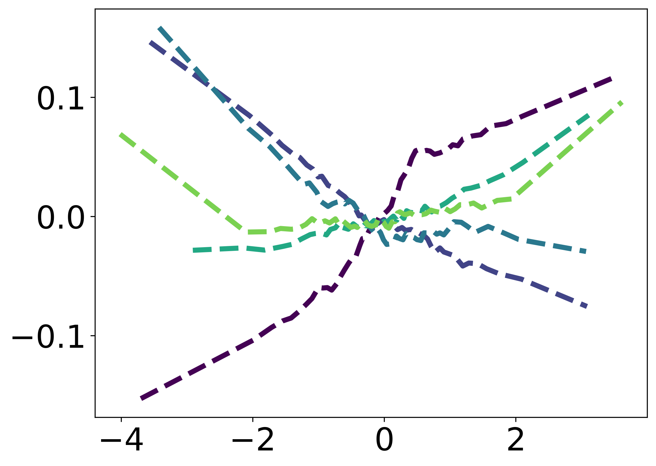
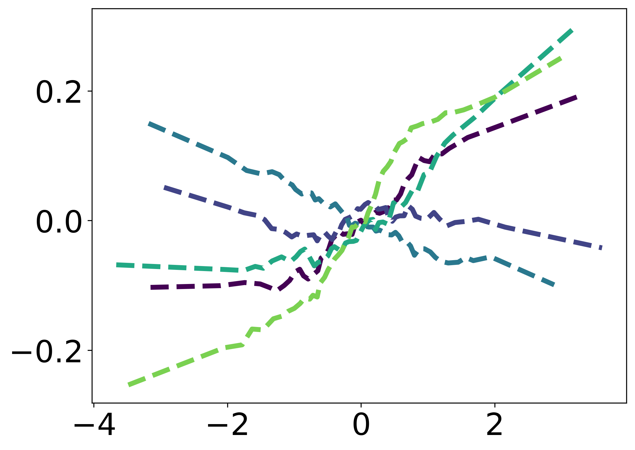
To further assess and explain these relative performance differences, we wish to inspect the prediction surface of a fitted TabPFN model. To do this, we make use of Accumulated Local Effects (ALE) plots, which summarize the dependence of the model on each individual feature [2].777ALE plots avoid both the confounding associated with conditional dependence plots and the out-of-sample instability associated with marginal dependence plots. Figure 17 exhibits the results when the features are orthogonal. We observe that for moderate to high SNR (), almost all ALE plots of relevant features are roughly linear. In addition, when , the ALE plots for the irrelevant features display much less variation, which suggests that the TabPFN model is indeed well-approximated by a low-dimensional linear surface. For smaller SNR, the ALE plots are generally nonlinear and are not shown.
To further quantify the faithfulness of the linear approximation in the settings identified above (, ), we fit an ordinary least squares model to the TabPFN predicted values using only the relevant features. As shown in the Table 2, the resulting test set values are at least . Furthermore, we can treat the regression coefficients of the linear approximation as estimates of the true regression coefficients. The bias and variance of these estimates are also shown in Table 2. For high to moderate sparsity, we observe that the TabPFN coefficients have smaller bias compared to the LASSO coefficients. Although we report squared bias, we note that all bias values are negative. We thus observe that TabPFN is able to avoid the well-known tendency of LASSO to bias its estimates via shrinkage.

| SNR | TabPFN | LASSO | |||||
|---|---|---|---|---|---|---|---|
| Bias2 | Var | Bias2 | Var | ||||
| 1.22 | 1 | 0.9960 | 0.0001 | 0.0017 | 1.0000 | 0.0076 | 0.0020 |
| 5 | 0.9917 | 0.0007 | 0.0087 | 1.0000 | 0.0201 | 0.0087 | |
| 10 | 0.9774 | 0.0035 | 0.0188 | 1.0000 | 0.0271 | 0.0173 | |
| 20 | 0.9566 | 0.0191 | 0.0502 | 1.0000 | 0.0329 | 0.0362 | |
| 30 | 0.9409 | 0.0435 | 0.0779 | 1.0000 | 0.0309 | 0.0551 | |
| 6 | 1 | 0.9990 | 0.0000 | 0.0004 | 1.0000 | 0.0015 | 0.0004 |
| 5 | 0.9975 | 0.0001 | 0.0018 | 1.0000 | 0.0041 | 0.0018 | |
| 10 | 0.9939 | 0.0007 | 0.0036 | 1.0000 | 0.0055 | 0.0035 | |
| 20 | 0.9870 | 0.0036 | 0.0091 | 1.0000 | 0.0067 | 0.0074 | |
| 30 | 0.9800 | 0.0089 | 0.0177 | 1.0000 | 0.0062 | 0.0112 | |
4.3 Robustness-efficiency trade-offs in classification
In our last experiment, we examine the classification performance of TabPFN in the presence of label noise, that is, when the observed labels in our training set are corrupted from their true values , such as by coding errors. For simplicity, we consider homogeneous noise in a binary class setting:
where is the corruption fraction. The goal is to train a classifier to predict the original label. In other words, we want to estimate a mapping minimizing the risk
This problem is especially interesting when the conditional distribution of the true label, , has a simple parametric form. For example, if is Gaussian, the noise-free classification problem can be solved efficiently via linear discriminant analysis (LDA). On the other hand, the conditional distribution of the corrupted label, , does not have the correct functional form, which makes LDA inconsistent. In comparison, Cannings, Fan and Samworth [8] proved that -nearest neighbors (NN) and kernelized support vector machines (SVM) can be robust to label noise. However, these methods, which are based on local averaging, pay a price in terms of being less efficient when the labels are noise free.
We show that TabPFN is able to break this robustness-efficiency trade-off. On the one hand, it remains consistent in the presence of label noise. On the other hand, it is more efficient than NN, SVM and even LDA across all simulation settings, including when there is no label noise.
4.3.1 Experimental design.
Following Cannings, Fan and Samworth [8], we generate data from two models:
-
M1
with , where .
-
M2
with .
For each model, we generate an IID sample of size , reserving the first observations for training and the remaining for testing. For the training set, we set . The optimal Bayes classifier minimizes this risk:
where . For any classifier , we define its excess risk as .
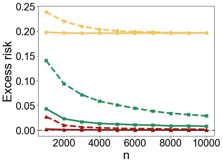
We compare four classifiers: Bayes, -NN, LDA, and TabPFN. For the Bayes classifier, the true is used in evaluation, and this serves as the gold standard for comparison. Each of the remaining classifiers is trained on two versions of the data: a clean training set and a noise-corrupted version. The resulting classifiers are named accordingly. Details such as hyper-parameter selection are deferred to Appendix F. This process is repeated 1000 times, with Figure 6 showing the average excess risk across repetitions.
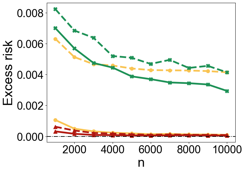
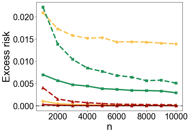
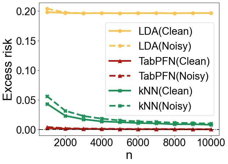
4.3.2 Prediction performance comparison.
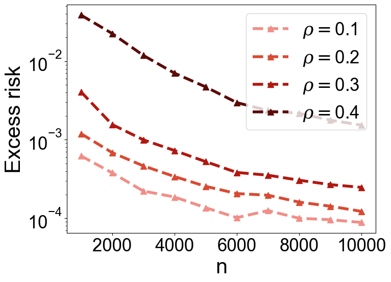
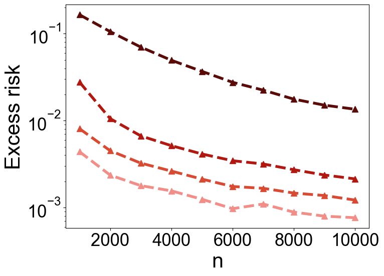
Under both generative models, TabPFN (clean) performs as well as the optimal Bayes classifier when the training set size is bigger than K. TabPFN (noisy) shows slightly worse performance than its clean-data counterpart but demonstrates exceptional robustness to label noise in all cases while maintaining high accuracy. Even with noise levels as high as , TabPFN (noisy) nearly matches the optimal classifier given a sufficiently large training set (K samples). LDA exhibits no robustness under M1 and performs poorly under M2 due to the nonlinear Bayes decision boundary. While the -NN classifier shows some consistency—particularly under M2 with low noise levels—it is less robust than TabPFN in other scenarios. Moreover, Figure 7 demonstrates that TabPFN remains robust even at . Interestingly, we notice that there is a significant performance gap between and for small training set sizes.
5 Discussion
5.1 Foundation models
In 2021, Bommasani et al. [6] coined the term “foundation model” to refer to “any model that is trained on broad data (generally using self-supervision at scale) that can be adapted (e.g., fine-tuned) to a wide range of downstream tasks”. They also noted a paradigm shift in artificial intelligence which de-prioritized the development of task-specific models in favor of building these foundation models, with LLMs being the most prominent examples. Until recently, the modality of tabular data has resisted this trend, but the tide may be turning. Hollmann et al. [20] provided a proof-of-concept that, in addition to regression and classification, TabPFN can support “data generation, density estimation, learning reusable embeddings and fine-tuning”, consequently claiming that TabPFN is a tabular foundation model.888These capabilities were not fully investigated by Hollmann et al. [20] and some are not supported by their publicly available code at the time of writing. Our investigations support this claim by showing that simple applications of TabPFN can surpass state-of-the-art approaches to some statistical estimation problems.
These studies are of course preliminary—our numerical experiments made exclusive use of synthetic data—and we do not suggest that TabPFN is a perfect model—it seems to struggle with dense regression, cannot handle features, and has MSE curves which seem to plateau for samples [27]. On the other hand, the evidence suggests that tabular foundation models are not only possible, but can surpass existing modeling approaches on a wide range of statistical tasks, possibly touching on all areas of statistics. In addition, Van Breugel and Van Der Schaar [39] have a bold vision of tabular foundational models being able to perform automatic meta-analyses, out-of-domain simulation, and other tasks for which adequate methodology does not yet exist. This line of thinking—that there may one day be one model to rule them all—is of course contrary to mainstream statistical thinking, which has traditionally emphasized bespoke models for different problems. Just as AI scientists continue to wrestle with the academic and societal consequences of the emergence of foundation models, statisticians may also be forced to confront profound changes in our field.
5.2 In-context learning
Another way in which TabPFN challenges current statistical thinking is via its illustration of the power of “in-context learning”, whose historical development we now discuss. In a landmark paper, Brown et al. [7] studied the LLM GPT-3 and discovered that it could learn how to perform tasks (e.g., language translation) that it was not explicitly trained to do and without changing any of the model’s parameters, simply by providing examples of the task in a prompt (text input) to the model. They called this ability “in-context learning” (ICL). Garg et al. [15] later framed ICL as a statistical learning problem. Under their framework, a prompt is a random sequence , where are drawn IID from a covariate distribution and is drawn from a distribution over a function class . A model is a fixed mapping from prompts to the (real-valued) label space and is said to have learned in-context (with respect to ) if for some tolerance and loss function . Garg et al. [15] was able to show via numerical experiments that a transformer, trained from scratch on IID prompts generated as described above, could successfully learn simple function classes (e.g. linear functions) in-context, inspiring a wave of theoretical interest in the problem [44, 4, 23].
On the other hand, it seems that Brown et al. [7] and Garg et al. [15]’s definitions of ICL are respectively too broad and too narrow to capture the scope of the learning strategy employed by TabPFN and other recent work claiming to implement ICL to solve statistical estimation problems. These include causal discovery [12], posterior inference for generalized linear models, factor models, and Gaussian mixture models [34], RNA folding time density estimation [36], and Poisson mean estimation under empirical Bayes [38]. None of these works provide a definition of ICL, but we find that the common denominator is that they train a transformer model using a large number of synthetic datasets to learn a mapping on the space of datasets. The target of the mapping can be a causal graph, a posterior distribution on parameter vector, or a Poisson mean vector estimate. In each of these problems, the ICL approach is shown to achieve higher accuracy than state-of-the-art methods, such as variational inference for posterior approximation, or non-parametric maximum-likelihood estimation in the case of empirical Bayes.
5.3 Future directions
These advances present both opportunities and challenges for the statistical community. TabPFN’s success stems from a synthesis of ideas across disciplines, coupled with non-trivial engineering efforts. The current version [20] builds on its predecessor [19], with key improvements in (1) prior data generation and (2) transformer architecture—both empirically shown to enhance performance. As statisticians, we can contribute to this evolving field by addressing critical questions:
-
•
Interpretability & theoretical foundations: Transformers, with millions of parameters, often lack interpretability. Understanding when TabPFN succeeds or fails—along with its statistical guarantees—remains an open problem.
-
•
Reliability in practice: While TabPFN and related methods show promise as off-the-shelf tools for biomedical and other applications, their real-world reliability—particularly for inference tasks—requires rigorous evaluation.
-
•
Scalability & limitations: Current implementations struggle with dense/high-dimensional regression and K samples. Addressing this bottleneck is essential for broader applicability. Recent work like [33] offers preliminary solutions, but fundamental constraints remain.
[Acknowledgments] This research was enabled in part by support provided by Cedar (cedar.alliancecan.ca) and the Digital Research Alliance of Canada (alliancecan.ca). The authors would like to thank Krishnakumar Balasubramanian, Arik Reuter, Chandan Singh, and Yuqian Zhang for useful discussions.
Qiong Zhang is supported by the National Key R&D Program of China Grant 2024YFA1015800 and National Natural Science Foundation of China Grant 12301391. Yan Shuo Tan is supported by NUS Start-up Grant A-8000448-00-00 and MOE AcRF Tier 1 Grant A-8002498-00-00. Qinglong Tian and Pengfei Li are supported by the Natural Sciences and Engineering Research Council of Canada (RGPIN-2023-03479 and RGPIN-2020-04964).
References
- Angelopoulos et al. [2023] {barticle}[author] \bauthor\bsnmAngelopoulos, \bfnmAnastasios N\binitsA. N., \bauthor\bsnmBates, \bfnmStephen\binitsS., \bauthor\bsnmFannjiang, \bfnmClara\binitsC., \bauthor\bsnmJordan, \bfnmMichael I\binitsM. I. and \bauthor\bsnmZrnic, \bfnmTijana\binitsT. (\byear2023). \btitlePrediction-powered inference. \bjournalScience \bvolume382 \bpages669–674. \endbibitem
- Apley and Zhu [2020] {barticle}[author] \bauthor\bsnmApley, \bfnmDaniel W.\binitsD. W. and \bauthor\bsnmZhu, \bfnmJingyu\binitsJ. (\byear2020). \btitleVisualizing the effects of predictor variables in black box supervised learning models. \bjournalJournal of the Royal Statistical Society Series B: Statistical Methodology \bvolume82 \bpages1059-1086. \endbibitem
- Azriel et al. [2022] {barticle}[author] \bauthor\bsnmAzriel, \bfnmDavid\binitsD., \bauthor\bsnmBrown, \bfnmLawrence D\binitsL. D., \bauthor\bsnmSklar, \bfnmMichael\binitsM., \bauthor\bsnmBerk, \bfnmRichard\binitsR., \bauthor\bsnmBuja, \bfnmAndreas\binitsA. and \bauthor\bsnmZhao, \bfnmLinda\binitsL. (\byear2022). \btitleSemi-supervised linear regression. \bjournalJournal of the American Statistical Association \bvolume117 \bpages2238–2251. \endbibitem
- Bai et al. [2023] {barticle}[author] \bauthor\bsnmBai, \bfnmYu\binitsY., \bauthor\bsnmChen, \bfnmFan\binitsF., \bauthor\bsnmWang, \bfnmHuan\binitsH., \bauthor\bsnmXiong, \bfnmCaiming\binitsC. and \bauthor\bsnmMei, \bfnmSong\binitsS. (\byear2023). \btitleTransformers as statisticians: provable in-context learning with in-context algorithm selection. \bjournalAdvances in Neural Information Processing Systems \bvolume36 \bpages57125–57211. \endbibitem
- Battocchi et al. [2019] {bmisc}[author] \bauthor\bsnmBattocchi, \bfnmKeith\binitsK., \bauthor\bsnmDillon, \bfnmEleanor\binitsE., \bauthor\bsnmHei, \bfnmMaggie\binitsM., \bauthor\bsnmLewis, \bfnmGreg\binitsG., \bauthor\bsnmOka, \bfnmPaul\binitsP., \bauthor\bsnmOprescu, \bfnmMiruna\binitsM. and \bauthor\bsnmSyrgkanis, \bfnmVasilis\binitsV. (\byear2019). \btitleEconML: a Python package for ML-based heterogeneous treatment effects estimation. \bhowpublishedhttps://github.com/py-why/EconML. \bnoteVersion 0.x. \endbibitem
- Bommasani et al. [2021] {barticle}[author] \bauthor\bsnmBommasani, \bfnmRishi\binitsR., \bauthor\bsnmHudson, \bfnmDrew A\binitsD. A., \bauthor\bsnmAdeli, \bfnmEhsan\binitsE., \bauthor\bsnmAltman, \bfnmRuss\binitsR., \bauthor\bsnmArora, \bfnmSimran\binitsS., \bauthor\bparticlevon \bsnmArx, \bfnmSydney\binitsS., \bauthor\bsnmBernstein, \bfnmMichael S\binitsM. S., \bauthor\bsnmBohg, \bfnmJeannette\binitsJ., \bauthor\bsnmBosselut, \bfnmAntoine\binitsA., \bauthor\bsnmBrunskill, \bfnmEmma\binitsE. \betalet al. (\byear2021). \btitleOn the opportunities and risks of foundation models. \bjournalarXiv preprint arXiv:2108.07258. \endbibitem
- Brown et al. [2020] {barticle}[author] \bauthor\bsnmBrown, \bfnmTom\binitsT., \bauthor\bsnmMann, \bfnmBenjamin\binitsB., \bauthor\bsnmRyder, \bfnmNick\binitsN., \bauthor\bsnmSubbiah, \bfnmMelanie\binitsM., \bauthor\bsnmKaplan, \bfnmJared D\binitsJ. D., \bauthor\bsnmDhariwal, \bfnmPrafulla\binitsP., \bauthor\bsnmNeelakantan, \bfnmArvind\binitsA., \bauthor\bsnmShyam, \bfnmPranav\binitsP., \bauthor\bsnmSastry, \bfnmGirish\binitsG., \bauthor\bsnmAskell, \bfnmAmanda\binitsA. \betalet al. (\byear2020). \btitleLanguage models are few-shot learners. \bjournalAdvances in Neural Information Processing Systems \bvolume33 \bpages1877–1901. \endbibitem
- Cannings, Fan and Samworth [2020] {barticle}[author] \bauthor\bsnmCannings, \bfnmTimothy I\binitsT. I., \bauthor\bsnmFan, \bfnmYingying\binitsY. and \bauthor\bsnmSamworth, \bfnmRichard J\binitsR. J. (\byear2020). \btitleClassification with imperfect training labels. \bjournalBiometrika \bvolume107 \bpages311–330. \endbibitem
- Caruana, Karampatziakis and Yessenalina [2008] {binproceedings}[author] \bauthor\bsnmCaruana, \bfnmRich\binitsR., \bauthor\bsnmKarampatziakis, \bfnmNikos\binitsN. and \bauthor\bsnmYessenalina, \bfnmAinur\binitsA. (\byear2008). \btitleAn empirical evaluation of supervised learning in high dimensions. In \bbooktitleProceedings of the 25th International Conference on Machine learning \bpages96–103. \endbibitem
- Chakrabortty and Cai [2018] {barticle}[author] \bauthor\bsnmChakrabortty, \bfnmAbhishek\binitsA. and \bauthor\bsnmCai, \bfnmTianxi\binitsT. (\byear2018). \btitleEfficient and adaptive linear regression in semi-supervised settings. \bjournalThe Annals of Statistics \bvolume46 \bpages1541 – 1572. \endbibitem
- Chipman, George and McCulloch [2010] {barticle}[author] \bauthor\bsnmChipman, \bfnmHugh A\binitsH. A., \bauthor\bsnmGeorge, \bfnmEdward I\binitsE. I. and \bauthor\bsnmMcCulloch, \bfnmRobert E\binitsR. E. (\byear2010). \btitleBART: Bayesian additive regression trees. \bjournalThe Annals of Applied Statistics \bvolume4 \bpages266–298. \endbibitem
- Dhir et al. [2025] {binproceedings}[author] \bauthor\bsnmDhir, \bfnmAnish\binitsA., \bauthor\bsnmAshman, \bfnmMatthew\binitsM., \bauthor\bsnmRequeima, \bfnmJames\binitsJ. and \bauthor\bparticlevan der \bsnmWilk, \bfnmMark\binitsM. (\byear2025). \btitleA meta-learning approach to Bayesian causal discovery. In \bbooktitleThe Thirteenth International Conference on Learning Representations. \endbibitem
- Fernández-Delgado et al. [2014] {barticle}[author] \bauthor\bsnmFernández-Delgado, \bfnmManuel\binitsM., \bauthor\bsnmCernadas, \bfnmEva\binitsE., \bauthor\bsnmBarro, \bfnmSenén\binitsS. and \bauthor\bsnmAmorim, \bfnmDinani\binitsD. (\byear2014). \btitleDo we need hundreds of classifiers to solve real world classification problems? \bjournalThe Journal of Machine Learning Research \bvolume15 \bpages3133–3181. \endbibitem
- Foster and Syrgkanis [2023] {barticle}[author] \bauthor\bsnmFoster, \bfnmDylan J\binitsD. J. and \bauthor\bsnmSyrgkanis, \bfnmVasilis\binitsV. (\byear2023). \btitleOrthogonal statistical learning. \bjournalThe Annals of Statistics \bvolume51 \bpages879–908. \endbibitem
- Garg et al. [2022] {barticle}[author] \bauthor\bsnmGarg, \bfnmShivam\binitsS., \bauthor\bsnmTsipras, \bfnmDimitris\binitsD., \bauthor\bsnmLiang, \bfnmPercy S\binitsP. S. and \bauthor\bsnmValiant, \bfnmGregory\binitsG. (\byear2022). \btitleWhat can transformers learn in-context? a case study of simple function classes. \bjournalAdvances in Neural Information Processing Systems \bvolume35 \bpages30583–30598. \endbibitem
- Garnelo et al. [2018] {barticle}[author] \bauthor\bsnmGarnelo, \bfnmMarta\binitsM., \bauthor\bsnmSchwarz, \bfnmJonathan\binitsJ., \bauthor\bsnmRosenbaum, \bfnmDan\binitsD., \bauthor\bsnmViola, \bfnmFabio\binitsF., \bauthor\bsnmRezende, \bfnmDanilo J\binitsD. J., \bauthor\bsnmEslami, \bfnmSM\binitsS. and \bauthor\bsnmTeh, \bfnmYee Whye\binitsY. W. (\byear2018). \btitleNeural processes. \bjournalarXiv preprint arXiv:1807.01622. \endbibitem
- Grinsztajn, Oyallon and Varoquaux [2022] {barticle}[author] \bauthor\bsnmGrinsztajn, \bfnmLéo\binitsL., \bauthor\bsnmOyallon, \bfnmEdouard\binitsE. and \bauthor\bsnmVaroquaux, \bfnmGaël\binitsG. (\byear2022). \btitleWhy do tree-based models still outperform deep learning on typical tabular data? \bjournalAdvances in Neural Information Processing Systems \bvolume35 \bpages507–520. \endbibitem
- Hastie, Tibshirani and Tibshirani [2020] {barticle}[author] \bauthor\bsnmHastie, \bfnmTrevor\binitsT., \bauthor\bsnmTibshirani, \bfnmRobert\binitsR. and \bauthor\bsnmTibshirani, \bfnmRyan\binitsR. (\byear2020). \btitleBest subset, forward stepwise or lasso? Analysis and recommendations based on extensive comparisons. \bjournalStatistical Science \bvolume35 \bpages579–592. \endbibitem
- Hollmann et al. [2022] {binproceedings}[author] \bauthor\bsnmHollmann, \bfnmNoah\binitsN., \bauthor\bsnmMüller, \bfnmSamuel\binitsS., \bauthor\bsnmEggensperger, \bfnmKatharina\binitsK. and \bauthor\bsnmHutter, \bfnmFrank\binitsF. (\byear2022). \btitleTabPFN: a transformer that solves small tabular classification problems in a second. In \bbooktitleNeurIPS 2022 First Table Representation Workshop. \endbibitem
- Hollmann et al. [2025] {barticle}[author] \bauthor\bsnmHollmann, \bfnmNoah\binitsN., \bauthor\bsnmMüller, \bfnmSamuel\binitsS., \bauthor\bsnmPurucker, \bfnmLennart\binitsL., \bauthor\bsnmKrishnakumar, \bfnmArjun\binitsA., \bauthor\bsnmKörfer, \bfnmMax\binitsM., \bauthor\bsnmHoo, \bfnmShi Bin\binitsS. B., \bauthor\bsnmSchirrmeister, \bfnmRobin Tibor\binitsR. T. and \bauthor\bsnmHutter, \bfnmFrank\binitsF. (\byear2025). \btitleAccurate predictions on small data with a tabular foundation model. \bjournalNature \bvolume637 \bpages319–326. \endbibitem
- Kawakita and Kanamori [2013] {barticle}[author] \bauthor\bsnmKawakita, \bfnmMasanori\binitsM. and \bauthor\bsnmKanamori, \bfnmTakafumi\binitsT. (\byear2013). \btitleSemi-supervised learning with density-ratio estimation. \bjournalMachine Learning \bvolume91 \bpages189–209. \endbibitem
- Kennedy [2023] {barticle}[author] \bauthor\bsnmKennedy, \bfnmEdward H.\binitsE. H. (\byear2023). \btitleTowards optimal doubly robust estimation of heterogeneous causal effects. \bjournalElectronic Journal of Statistics \bvolume17 \bpages3008 – 3049. \endbibitem
- Kim, Nakamaki and Suzuki [2024] {barticle}[author] \bauthor\bsnmKim, \bfnmJuno\binitsJ., \bauthor\bsnmNakamaki, \bfnmTai\binitsT. and \bauthor\bsnmSuzuki, \bfnmTaiji\binitsT. (\byear2024). \btitleTransformers are minimax optimal nonparametric in-context learners. \bjournalAdvances in Neural Information Processing Systems \bvolume37 \bpages106667–106713. \endbibitem
- Künzel et al. [2019] {barticle}[author] \bauthor\bsnmKünzel, \bfnmSören R\binitsS. R., \bauthor\bsnmSekhon, \bfnmJasjeet S\binitsJ. S., \bauthor\bsnmBickel, \bfnmPeter J\binitsP. J. and \bauthor\bsnmYu, \bfnmBin\binitsB. (\byear2019). \btitleMetalearners for estimating heterogeneous treatment effects using machine learning. \bjournalProceedings of the National Academy of Sciences \bvolume116 \bpages4156–4165. \endbibitem
- Ma, Pathak and Wainwright [2023] {barticle}[author] \bauthor\bsnmMa, \bfnmCong\binitsC., \bauthor\bsnmPathak, \bfnmReese\binitsR. and \bauthor\bsnmWainwright, \bfnmMartin J.\binitsM. J. (\byear2023). \btitleOptimally tackling covariate shift in RKHS-based nonparametric regression. \bjournalThe Annals of Statistics \bvolume51 \bpages738 – 761. \endbibitem
- Müller et al. [2022] {binproceedings}[author] \bauthor\bsnmMüller, \bfnmSamuel\binitsS., \bauthor\bsnmHollmann, \bfnmNoah\binitsN., \bauthor\bsnmArango, \bfnmSebastian Pineda\binitsS. P., \bauthor\bsnmGrabocka, \bfnmJosif\binitsJ. and \bauthor\bsnmHutter, \bfnmFrank\binitsF. (\byear2022). \btitleTransformers can do Bayesian inference. In \bbooktitleInternational Conference on Learning Representations. \endbibitem
- Nagler [2023] {binproceedings}[author] \bauthor\bsnmNagler, \bfnmThomas\binitsT. (\byear2023). \btitleStatistical foundations of prior-data fitted networks. In \bbooktitleProceedings of the 40th International Conference on Machine Learning. \bseriesProceedings of Machine Learning Research \bvolume202 \bpages25660–25676. \bpublisherPMLR. \endbibitem
- Nie and Wager [2020] {barticle}[author] \bauthor\bsnmNie, \bfnmX\binitsX. and \bauthor\bsnmWager, \bfnmS\binitsS. (\byear2020). \btitleQuasi-oracle estimation of heterogeneous treatment effects. \bjournalBiometrika \bvolume108 \bpages299-319. \endbibitem
- Olson et al. [2018] {binproceedings}[author] \bauthor\bsnmOlson, \bfnmRandal S\binitsR. S., \bauthor\bsnmCava, \bfnmWilliam La\binitsW. L., \bauthor\bsnmMustahsan, \bfnmZairah\binitsZ., \bauthor\bsnmVarik, \bfnmAkshay\binitsA. and \bauthor\bsnmMoore, \bfnmJason H\binitsJ. H. (\byear2018). \btitleData-driven advice for applying machine learning to bioinformatics problems. In \bbooktitleBiocomputing 2018: Proceedings of the Pacific Symposium \bpages192–203. \bpublisherWorld Scientific. \endbibitem
- Pearl [2009] {bbook}[author] \bauthor\bsnmPearl, \bfnmJudea\binitsJ. (\byear2009). \btitleCausality. \bpublisherCambridge university press. \endbibitem
- Qin et al. [2025] {barticle}[author] \bauthor\bsnmQin, \bfnmJing\binitsJ., \bauthor\bsnmLiu, \bfnmYukun\binitsY., \bauthor\bsnmLi, \bfnmMoming\binitsM. and \bauthor\bsnmand, \bfnmChiung-Yu Huang\binitsC.-Y. H. (\byear2025). \btitleDistribution-free prediction intervals under covariate shift, with an application to causal inference. \bjournalJournal of the American Statistical Association \bvolume120 \bpages559–571. \endbibitem
- Qiu, Dobriban and Tchetgen Tchetgen [2023] {barticle}[author] \bauthor\bsnmQiu, \bfnmHongxiang\binitsH., \bauthor\bsnmDobriban, \bfnmEdgar\binitsE. and \bauthor\bsnmTchetgen Tchetgen, \bfnmEric\binitsE. (\byear2023). \btitlePrediction sets adaptive to unknown covariate shift. \bjournalJournal of the Royal Statistical Society Series B: Statistical Methodology \bvolume85 \bpages1680–1705. \endbibitem
- Qu et al. [2025] {barticle}[author] \bauthor\bsnmQu, \bfnmJingang\binitsJ., \bauthor\bsnmHolzmüller, \bfnmDavid\binitsD., \bauthor\bsnmVaroquaux, \bfnmGaël\binitsG. and \bauthor\bsnmMorvan, \bfnmMarine Le\binitsM. L. (\byear2025). \btitleTabICL: a tabular foundation model for in-context learning on large data. \bjournalarXiv preprint arXiv:2502.05564. \endbibitem
- Reuter et al. [2025] {barticle}[author] \bauthor\bsnmReuter, \bfnmArik\binitsA., \bauthor\bsnmRudner, \bfnmTim GJ\binitsT. G., \bauthor\bsnmFortuin, \bfnmVincent\binitsV. and \bauthor\bsnmRügamer, \bfnmDavid\binitsD. (\byear2025). \btitleCan transformers learn full Bayesian inference in context? \bjournalarXiv preprint arXiv:2501.16825. \endbibitem
- Rubin [1974] {barticle}[author] \bauthor\bsnmRubin, \bfnmDonald B\binitsD. B. (\byear1974). \btitleEstimating causal effects of treatments in randomized and nonrandomized studies. \bjournalJournal of Educational Psychology \bvolume66 \bpages688. \endbibitem
- Scheuer et al. [2025] {binproceedings}[author] \bauthor\bsnmScheuer, \bfnmDominik\binitsD., \bauthor\bsnmRunge, \bfnmFrederic\binitsF., \bauthor\bsnmFranke, \bfnmJörg K. H.\binitsJ. K. H., \bauthor\bsnmWolfinger, \bfnmMichael T.\binitsM. T., \bauthor\bsnmFlamm, \bfnmChristoph\binitsC. and \bauthor\bsnmHutter, \bfnmFrank\binitsF. (\byear2025). \btitleKinPFN: Bayesian approximation of RNA folding kinetics using prior-data fitted networks. In \bbooktitleThe Thirteenth International Conference on Learning Representations. \endbibitem
- Song, Lin and Zhou [2024] {barticle}[author] \bauthor\bsnmSong, \bfnmShanshan\binitsS., \bauthor\bsnmLin, \bfnmYuanyuan\binitsY. and \bauthor\bsnmZhou, \bfnmYong\binitsY. (\byear2024). \btitleA general M-estimation theory in semi-supervised framework. \bjournalJournal of the American Statistical Association \bvolume119 \bpages1065–1075. \endbibitem
- Teh, Jabbour and Polyanskiy [2025] {barticle}[author] \bauthor\bsnmTeh, \bfnmAnzo\binitsA., \bauthor\bsnmJabbour, \bfnmMark\binitsM. and \bauthor\bsnmPolyanskiy, \bfnmYury\binitsY. (\byear2025). \btitleSolving empirical Bayes via transformers. \bjournalarXiv preprint arXiv:2502.09844. \endbibitem
- Van Breugel and Van Der Schaar [2024] {binproceedings}[author] \bauthor\bsnmVan Breugel, \bfnmBoris\binitsB. and \bauthor\bsnmVan Der Schaar, \bfnmMihaela\binitsM. (\byear2024). \btitlePosition: why tabular foundation models should be a research priority. In \bbooktitleProceedings of the 41st International Conference on Machine Learning. \bseriesProceedings of Machine Learning Research \bvolume235 \bpages48976–48993. \bpublisherPMLR. \endbibitem
- Vaswani et al. [2017] {barticle}[author] \bauthor\bsnmVaswani, \bfnmAshish\binitsA., \bauthor\bsnmShazeer, \bfnmNoam\binitsN., \bauthor\bsnmParmar, \bfnmNiki\binitsN., \bauthor\bsnmUszkoreit, \bfnmJakob\binitsJ., \bauthor\bsnmJones, \bfnmLlion\binitsL., \bauthor\bsnmGomez, \bfnmAidan N\binitsA. N., \bauthor\bsnmKaiser, \bfnmŁukasz\binitsŁ. and \bauthor\bsnmPolosukhin, \bfnmIllia\binitsI. (\byear2017). \btitleAttention is all you need. \bjournalAdvances in Neural Information Processing Systems \bvolume30. \endbibitem
- Wang [2024] {barticle}[author] \bauthor\bsnmWang, \bfnmKaizheng\binitsK. (\byear2024). \btitlePseudo-labeling for kernel ridge regression under covariate shift. \bjournalarXiv preprint arXiv:2302.10160. \endbibitem
- Wang et al. [2021] {barticle}[author] \bauthor\bsnmWang, \bfnmChi\binitsC., \bauthor\bsnmWu, \bfnmQingyun\binitsQ., \bauthor\bsnmWeimer, \bfnmMarkus\binitsM. and \bauthor\bsnmZhu, \bfnmErkang\binitsE. (\byear2021). \btitleFLAML: a fast and lightweight automl library. \bjournalProceedings of Machine Learning and Systems \bvolume3 \bpages434–447. \endbibitem
- Yang, Kuchibhotla and Tchetgen Tchetgen [2024] {barticle}[author] \bauthor\bsnmYang, \bfnmYachong\binitsY., \bauthor\bsnmKuchibhotla, \bfnmArun Kumar\binitsA. K. and \bauthor\bsnmTchetgen Tchetgen, \bfnmEric\binitsE. (\byear2024). \btitleDoubly robust calibration of prediction sets under covariate shift. \bjournalJournal of the Royal Statistical Society Series B: Statistical Methodology \bvolume86 \bpages943–965. \endbibitem
- Zhang, Frei and Bartlett [2024] {barticle}[author] \bauthor\bsnmZhang, \bfnmRuiqi\binitsR., \bauthor\bsnmFrei, \bfnmSpencer\binitsS. and \bauthor\bsnmBartlett, \bfnmPeter L\binitsP. L. (\byear2024). \btitleTrained transformers learn linear models in-context. \bjournalJournal of Machine Learning Research \bvolume25 \bpages1–55. \endbibitem
- Zhu [2010] {binbook}[author] \bauthor\bsnmZhu, \bfnmXiaojin\binitsX. (\byear2010). \btitleSemi-supervised learning. In \bbooktitleEncyclopedia of Machine Learning \bpages892–897. \bpublisherSpringer US, \baddressBoston, MA. \endbibitem
Appendix A Experiment details for semi-supervised estimation
We adopt the same experimental setup as in Song, Lin and Zhou [37]. For completeness, we detail the simulation settings in Section A.1 and present additional results in Section A.2.
A.1 Simulation settings
In correspondence with the three settings in Table 3, we describe the data-generating model for each setting respectively.
-
•
Linear regression working model. In this setting, the data is generated from
where and . The power and exponential operations on the vector are performed element-wise. We let , with and both being all-ones vectors.
-
•
Logistic regression working model. In this setting, the data is generated from
where and is a matrix with -th entry equal to . We set , as a vector of all s, and as a vector of all s.
-
•
Linear quantile regression working model. In this setting, the data is generated from
where , and . We set , , and , where and denote -dimensional all-ones and all-zeros vectors, respectively.
A.2 Additional simulation results
We include all the simulation results in Figures 8 to 13. With the sole exception of the case under logistic regression, TabPFN-I consistently outperforms all competing methods.


Appendix B Experiment details for causal inference
We provide the details for the causal inference experiment and the full experiment result in this section.
The specification of the feature distribution, propensity function, base function, and treatment effect function under all setups are given in Table 3.
| Setup | Propensity | Base | Effect |
|---|---|---|---|
These functions corresponding to the following setting:
-
•
Setup A: complicated and , but a relatively simple .
-
•
Setup B: randomized trial with a complex and .
-
•
Setup C: complex and , but a constant .
-
•
Setup D: response under treatment is independent of the response under control, and hence there is no statistical benefit of jointly learning the two responses.
-
•
Setup E: large resulting in substantial confounding, discontinuous .
-
•
Setup F: similar to setup , but with a smooth .
Our experiments are implemented using the econml [5] package in Python, we use the FLAML package [42] to implement all AutoML-based learners. We use the 5-fold cross-validation to choose the optimal algorithms and its corresponding hyperparameters for AutoML-based learners. We randomly generate data from each setting for times and the average test MSE over repetitions for CATE is reported in Table 4.
| Setup | N | DR | S | T | X | R | Oracle | |||||
|---|---|---|---|---|---|---|---|---|---|---|---|---|
| TabPFN | AutoML | TabPFN | AutoML | TabPFN | AutoML | TabPFN | AutoML | AutoML | AutoML | |||
| A | 500 | 0.5 | 0.0353 | 0.0459 | 0.0306 | 0.0451 | 0.0904 | 0.2367 | 0.0445 | 0.0592 | 0.0423 | 0.0527 |
| 1 | 0.0491 | 0.0720 | 0.0393 | 0.0537 | 0.1672 | 0.6091 | 0.0619 | 0.0920 | 0.0681 | 0.0803 | ||
| 2 | 0.0701 | 0.2610 | 0.0647 | 0.0666 | 0.4703 | 1.6589 | 0.1520 | 0.2904 | 0.1776 | 0.2072 | ||
| 1000 | 0.5 | 0.0358 | 0.0417 | 0.0345 | 0.0445 | 0.0603 | 0.1395 | 0.0379 | 0.0462 | 0.0408 | 0.0472 | |
| 1 | 0.0360 | 0.0519 | 0.0298 | 0.0513 | 0.1006 | 0.2939 | 0.0444 | 0.0651 | 0.0518 | 0.0559 | ||
| 2 | 0.0461 | 0.0923 | 0.0509 | 0.0578 | 0.2419 | 0.8325 | 0.0864 | 0.1311 | 0.1145 | 0.1090 | ||
| 2000 | 0.5 | 0.0379 | 0.0397 | 0.0369 | 0.0446 | 0.0545 | 0.0905 | 0.0376 | 0.0420 | 0.0399 | 0.0439 | |
| 1 | 0.0360 | 0.0412 | 0.0308 | 0.0468 | 0.0704 | 0.1536 | 0.0364 | 0.0467 | 0.0420 | 0.0473 | ||
| 2 | 0.0366 | 0.0593 | 0.0343 | 0.0474 | 0.1390 | 0.4325 | 0.0499 | 0.0690 | 0.0628 | 0.0699 | ||
| B | 500 | 0.5 | 0.9449 | 0.9726 | 0.8850 | 0.9161 | 1.0594 | 1.2249 | 0.9615 | 1.0196 | 0.9670 | 0.9316 |
| 1 | 0.9988 | 1.0338 | 0.8487 | 0.9256 | 1.2281 | 1.4780 | 1.0423 | 1.1467 | 1.0315 | 0.9917 | ||
| 2 | 1.1678 | 1.5120 | 0.8262 | 0.9279 | 1.5869 | 2.4374 | 1.2474 | 1.3836 | 1.3388 | 1.2320 | ||
| 1000 | 0.5 | 0.9236 | 0.9601 | 0.8957 | 0.9283 | 1.0003 | 1.0622 | 0.9317 | 0.9494 | 0.9633 | 0.9442 | |
| 1 | 0.9441 | 1.0354 | 0.8731 | 0.9327 | 1.0961 | 1.2457 | 0.9661 | 1.0426 | 0.9958 | 0.9811 | ||
| 2 | 1.0131 | 1.2884 | 0.8391 | 0.9405 | 1.3271 | 1.4817 | 1.0791 | 1.1271 | 1.0919 | 1.1219 | ||
| 2000 | 0.5 | 0.9127 | 0.9268 | 0.9051 | 0.9155 | 0.9776 | 1.0294 | 0.9240 | 0.9504 | 0.9263 | 0.9338 | |
| 1 | 0.9136 | 0.9475 | 0.8938 | 0.9226 | 1.0538 | 1.0820 | 0.9399 | 0.9784 | 0.9643 | 0.9552 | ||
| 2 | 0.9298 | 1.0576 | 0.8542 | 0.9218 | 1.1856 | 1.2973 | 0.9940 | 1.0053 | 1.0489 | 1.1005 | ||
| C | 500 | 0.5 | 0.9880 | 1.1573 | 1.0206 | 1.1170 | 1.1092 | 1.6273 | 1.0315 | 1.1741 | 1.1283 | 1.0428 |
| 1 | 1.0148 | 1.3708 | 1.0550 | 1.1556 | 1.3627 | 2.2214 | 1.1288 | 1.3321 | 1.2393 | 1.1755 | ||
| 2 | 1.2039 | 2.0873 | 1.1602 | 1.1513 | 2.6658 | 3.5575 | 1.5984 | 1.6721 | 1.8985 | 1.5429 | ||
| 1000 | 0.5 | 0.9637 | 1.0413 | 1.0157 | 1.0291 | 1.0450 | 1.3988 | 1.0100 | 1.1034 | 1.1083 | 1.0229 | |
| 1 | 0.9460 | 1.1973 | 1.0287 | 1.0447 | 1.1727 | 1.7895 | 1.0555 | 1.2451 | 1.1026 | 1.0677 | ||
| 2 | 0.9633 | 1.4033 | 1.0803 | 1.1057 | 1.6611 | 2.6587 | 1.2487 | 1.3752 | 1.2119 | 1.1597 | ||
| 2000 | 0.5 | 0.9340 | 1.0387 | 1.0003 | 1.0182 | 0.9863 | 1.1943 | 0.9663 | 1.0306 | 1.0254 | 0.9914 | |
| 1 | 0.8782 | 1.0625 | 0.9930 | 1.0291 | 1.0220 | 1.4187 | 0.9542 | 1.0955 | 1.0335 | 0.9766 | ||
| 2 | 0.7964 | 1.1085 | 0.9754 | 1.0132 | 1.1751 | 1.9187 | 0.9667 | 1.1881 | 1.0689 | 1.0376 | ||
| D | 500 | 0.5 | 0.3146 | 0.3325 | 0.3078 | 0.3186 | 0.3194 | 0.3688 | 0.3101 | 0.3119 | 0.3297 | 0.3309 |
| 1 | 0.3234 | 0.4091 | 0.3104 | 0.3252 | 0.3811 | 0.5066 | 0.3310 | 0.3577 | 0.3707 | 0.4057 | ||
| 2 | 0.3746 | 0.6602 | 0.3139 | 0.3291 | 0.4476 | 0.8520 | 0.3796 | 0.4848 | 0.5620 | 0.6171 | ||
| 1000 | 0.5 | 0.3144 | 0.3281 | 0.3055 | 0.3192 | 0.3033 | 0.3535 | 0.3087 | 0.3218 | 0.3204 | 0.3273 | |
| 1 | 0.3181 | 0.3387 | 0.3093 | 0.3224 | 0.3235 | 0.4137 | 0.3149 | 0.3412 | 0.3372 | 0.3445 | ||
| 2 | 0.3416 | 0.4274 | 0.3143 | 0.3244 | 0.3837 | 0.5984 | 0.3433 | 0.4147 | 0.4255 | 0.4038 | ||
| 2000 | 0.5 | 0.3199 | 0.3187 | 0.3066 | 0.3142 | 0.3108 | 0.3332 | 0.3102 | 0.3108 | 0.3139 | 0.3217 | |
| 1 | 0.3280 | 0.3294 | 0.3058 | 0.3153 | 0.3112 | 0.3492 | 0.3086 | 0.3234 | 0.3247 | 0.3297 | ||
| 2 | 0.3601 | 0.3617 | 0.3092 | 0.3268 | 0.3708 | 0.4832 | 0.3285 | 0.3554 | 0.3702 | 0.3604 | ||
| E | 500 | 0.5 | 0.9974 | 1.1572 | 1.0074 | 1.1970 | 1.2127 | 1.9554 | 1.0603 | 1.2616 | 1.1245 | 1.3844 |
| 1 | 1.0197 | 1.4416 | 1.0125 | 1.3366 | 1.5399 | 2.9947 | 1.1330 | 1.5996 | 1.2971 | 1.3954 | ||
| 2 | 1.1507 | 1.9310 | 1.0358 | 1.4765 | 3.3103 | 6.6586 | 1.6092 | 2.5715 | 2.3374 | 2.1096 | ||
| 1000 | 0.5 | 0.9799 | 1.0975 | 1.0063 | 1.1111 | 1.1177 | 1.4992 | 1.0463 | 1.1522 | 1.0671 | 1.3618 | |
| 1 | 0.9830 | 1.1957 | 1.0086 | 1.1500 | 1.2408 | 2.0187 | 1.0758 | 1.3126 | 1.1155 | 1.1570 | ||
| 2 | 1.0295 | 1.4467 | 1.0200 | 1.2581 | 2.0002 | 3.9269 | 1.2779 | 1.7394 | 1.2873 | 1.4020 | ||
| 2000 | 0.5 | 0.9727 | 1.0652 | 1.0045 | 1.1386 | 1.0880 | 1.3228 | 1.0290 | 1.0962 | 1.0190 | 2.5772 | |
| 1 | 0.9612 | 1.1088 | 1.0018 | 1.1134 | 1.1356 | 1.6436 | 1.0302 | 1.1732 | 1.0697 | 1.1482 | ||
| 2 | 0.9629 | 1.2134 | 0.9980 | 1.1899 | 1.4940 | 2.7234 | 1.0977 | 1.4617 | 1.2380 | 1.1930 | ||
| F | 500 | 0.5 | 0.9054 | 1.1490 | 0.9225 | 1.1626 | 1.1541 | 2.1184 | 0.9731 | 1.2382 | 1.0686 | 2.2406 |
| 1 | 0.9285 | 1.3720 | 0.9276 | 1.3698 | 1.4309 | 3.3303 | 1.0477 | 1.6814 | 1.3613 | 1.4709 | ||
| 2 | 1.0800 | 2.2924 | 0.9490 | 1.5328 | 3.2448 | 7.4794 | 1.5656 | 2.4827 | 2.4312 | 1.8548 | ||
| 1000 | 0.5 | 0.8856 | 1.0488 | 0.9227 | 1.0632 | 1.0674 | 1.5690 | 0.9577 | 1.0724 | 0.9831 | 4.0442 | |
| 1 | 0.8831 | 1.1311 | 0.9259 | 1.1132 | 1.1392 | 2.2563 | 0.9858 | 1.2539 | 1.0727 | 1.1675 | ||
| 2 | 0.9289 | 1.5002 | 0.9441 | 1.2673 | 1.8699 | 4.3611 | 1.2044 | 1.7225 | 1.4343 | 1.4565 | ||
| 2000 | 0.5 | 0.8665 | 0.9958 | 0.9185 | 1.0941 | 1.0345 | 1.2813 | 0.9315 | 1.0029 | 0.9412 | 5.4930 | |
| 1 | 0.8353 | 1.0804 | 0.9139 | 1.0236 | 1.0342 | 1.6587 | 0.9160 | 1.1017 | 0.9808 | 1.2046 | ||
| 2 | 0.8017 | 1.2459 | 0.9002 | 1.1631 | 1.3191 | 2.8504 | 0.9575 | 1.3335 | 1.0868 | 1.1103 | ||
Appendix C Covariate shift
Figure 14 shows the Setting (ii) results, where the methods maintain their relative performance ordering observed in Setting (i).
Appendix D How does TabPFN extrapolate?
We evaluate the interpolation and extrapolation behavior of TabPFN trained on data sampled from predefined functions, comparing its performance to Gaussian process regression (GPR) as a baseline. Experiments are conducted in both one-dimensional (1D) and two-dimensional (2D) settings.
D.1 Training data generation
1D case. The training set of size consists of features sampled uniformly over . Responses are generated as:
where is one of the following:
-
(i)
Linear function: ,
-
(ii)
Quadratic function: ,
-
(iii)
Step function: with ,
-
(iv)
A randomly generated piecewise-linear function with pieces on .
TabPFN is trained on this small dataset and prediction is made over the extended interval to assess both interpolation () and extrapolation () performance.
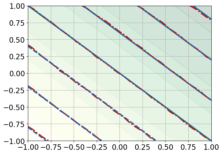
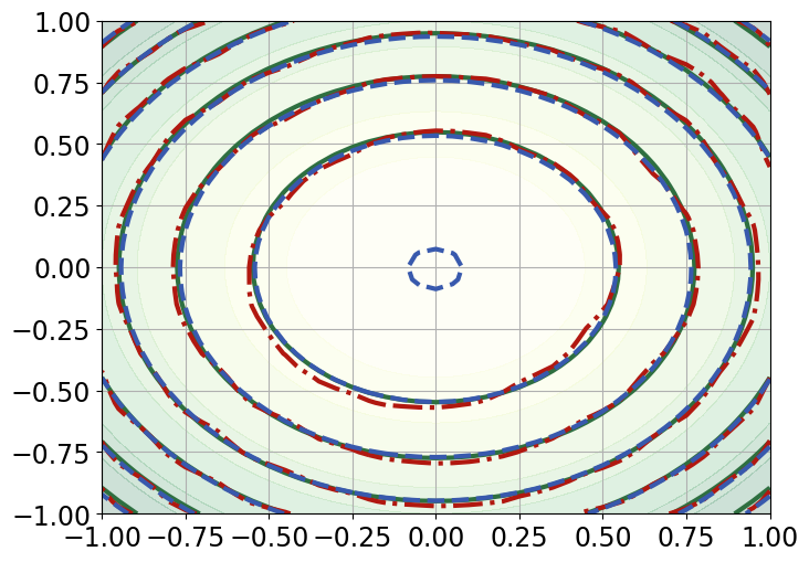
2D case. The training set consists of features , where and are each sampled uniformly from . These points form a mesh grid, resulting in total observations. We examine two cases: and . The responses are generated as:
where is analogously defined as in the 1D case:
-
(i)
Linear function: ,
-
(ii)
Quadratic function: ,
-
(iii)
Step function:
-
(iv)
Piecewise-bilinear function. Given a 2D grid of randomly generated function values of size . Uniformly divide into cells. For , find which cell it falls into. Suppose it falls into the th cell, compute the local coordinates:
and the bilinear function is given as
TabPFN is trained on this small dataset and prediction is made over the uniform mesh grid over to assess both interpolation () and extrapolation () performance.
D.2 Gaussian process regression
For both 1D and 2D cases, we compare TabPFN with Gaussian process regression (GPR). For Gaussian process regression, we consider kernels: constant kernel RBF kernel, constant kernel Matern kernel, constant kernel RationalQuadratic kernel, constant kernel ExpSineSquared kernel, constant kernel RBF kernel constant kernel Matern kernel. The candidate variance of the measurement error is over the grid . We maximize the marginal log-likelihood to select the optimal kernel and its corresponding optimal parameters, and the optimal measurement error variance. The optimal parameter for GPR is implemented using the GaussianProcessRegressor in sklearn package in Python.
D.3 Results
The results when under 1D case are visualized in Figure 15. The results under 2D case are visualized in Figure 16.
Appendix E Additional results for sparse linear regression
The ALE plots of TabPFN under sparse linear regression are given in this section in Figure 17.


Appendix F Implementation Details for LDA and kNN
When and , with , the optimal Bayes classifier takes the form:
The LDA classifier replaces population parameters with their sample estimates. Letting for clean training data, we compute:
yielding the LDA classifier:
For -nearest neighbors (NN) classification, we select the optimal number of neighbors via -fold cross-validation. The search grid consists of equally spaced integers between and , with the value maximizing cross-validation accuracy chosen for each experimental replication.