Efficient Gaussian Mixture Filters based on Transition Density Approximation
Abstract
Gaussian mixture filters for nonlinear systems usually rely on severe approximations when calculating mixtures in the prediction and filtering step. Thus, offline approximations of noise densities by Gaussian mixture densities to reduce the approximation error have been proposed. This results in exponential growth in the number of components, requiring ongoing component reduction, which is computationally complex. In this paper, the key idea is to approximate the true transition density by an axis-aligned Gaussian mixture, where two different approaches are derived. These approximations automatically ensure a constant number of components in the posterior densities without the need for explicit reduction. In addition, they allow a trade-off between estimation quality and computational complexity.
Index Terms:
Bayesian estimation, nonlinear systems, Gaussian mixture filter, transition density approximation.I Introduction
State estimation is a key element in many areas, such as tracking, guidance, positioning, navigation, sensor fusion, fault detection, and decision-making. Its goal is to estimate the state of a dynamic system, which is, in general, not directly measurable, from a set of noisy measurements.
State estimation began in the sixties with the introduction of the KF, which optimizes state estimation for linear systems by minimizing the mean square error. Its structure is followed by many algorithms addressing state estimation of nonlinear systems. The algorithms following the optimization approach provide point state estimates and covariance matrices of estimate errors. Another approach to state estimation uses Bayesian recursive relations, incorporating a Bayes equation and Chapman-Kolmogorov equation (CKE), to provide the state estimate as a conditional probability density function (PDF) based on a set of measurements. The conditional PDF completely describes the estimated state; however, the BRRs are analytically tractable only for a few special cases.
There are many approximate solutions to the BRRs leading to algorithms of various complexity. Assuming joint PDF of the state and measurement prediction Gaussian leads to a group called Gaussian filters (e.g., cubature filter [1] or the stochastic integration filter [2]), which are computationally light. However, the assumption seldom holds, and thus, GF performance for strongly nonlinear systems is poor.
Another group of approximate Bayesian algorithms results from discrete approximation of the posterior PDF. These include the point-mass filters [3] replacing the continuous support of the posterior by a grid of weighted points, which is usually orthogonal and equidistant. Such a grid is flexible in representing the posterior but results in computationally demanding algorithms due to the convolution calculated in the CKE. \Acppf [4] belong to the same group, but they replace the continuous support with a set of randomly positioned samples. They are computationally lighter than the PMFs, but the estimates are subject to random effects.
gmf [5] are Bayesian algorithms filling the gap between GFs and PMFs. The support of the posterior is continuous since they represent it by a mixture of Gaussian PDFs. The usage of a Gaussian mixture (GM) instead of a single Gaussian PDF results in better accuracy, even for highly nonlinear problems. This improvement occurs because each GM term has a small variance compared to the single Gaussian PDF, which mitigates the impact of strong nonlinearity. Compared to particle filters and PMFs, the Gaussian mixture filters are usually computationally lighter. For arbitrary nonlinear state and measurement equations, GMFs can be classified into two different approaches: local ones and global ones.
Local approaches process the GM components individually by a bank of filters, each processing a single component. This has been pioneered in [5] with the first use of GMs for Bayesian nonlinear filtering. The unavoidable increase in the number of components due to noises described by GMs is handled by simple neglecting and combination. In [6], a bank of Gaussian filters for the independent updates of Gaussian components is proposed with three different rules to update the component weights after the correction step.
A more recent discussion of weights calculation after the correction step based on prior linearization, posterior linearization, and without any linearization can be found in [7]. More complex individual filters have been used in [8], where a component-wise update is performed using a bank of Gaussian particle filters as proposed in [9].
Global approaches jointly process all the mixture components. An early global approach is the update step for prior GM with arbitrary nonlinear measurement equation in [10]. Instead of solving the complex problem of approximating the prior GM, a system of ordinary differential equations for posterior mixture parameters is solved over an artificial time interval. A recent global approach [11] considers the update step for a Gaussian mixture particle filter with deterministic samples. It works by drawing unweighted samples from the prior GM, assigning weights from the likelihood, computing higher-order moments from this sample-based posterior, and finally determining the posterior GM from moments while minimizing its Fisher information. This approach is based on calculating the Fisher information for GMs in [12].
Alternatively, global processing can be achieved with transition densities approximated by GMs, e.g., [13]. In general, for arbitrary mixtures, this leads to an exponential increase in the number of components over time in both the filtering and prediction steps. Usually, this is taken care of by regular mixture reduction, which is a non-convex and computationally complex optimization problem. To automatically limit the number of components in the prediction step with a GM transition density, [14] proposed to perform a decomposition into axis-aligned components. This not only allows a prespecified number of components without any reduction but also leads to closed-form expressions for the posterior mixture.
This paper follows the global processing and aims to propose GMF algorithms that impose the structure of the predictive and posterior PDF through a decomposition of the transition PDF to axis-aligned GMs. This allows the user to control accuracy and computational complexity by specifying the decomposition.
The paper is structured as follows: Section II introduces the state estimation problem, the BRRs, and their solution by the GMF. Section III describes two decompositions of the transition PDF leading to two proposed GMF algorithms described in Section IV. A numerical illustration of the developed algorithms is given in Section V, and Section VI provides concluding remarks.
II Bayesian state estimation and Gaussian mixture filter
Consider a discrete-time stochastic system described by a nonlinear state-space model
| (1a) | ||||
| (1b) | ||||
where and represent the immeasurable state of the system and the available measurement at time instant , respectively. The functions and are assumed known. The state noise and measurement noise are described by known PDFs and . The initial state is given by known PDF . Both noises are assumed to be white, mutually independent, and independent of the initial state.
II-A Bayesian state estimation
The goal of state estimation is to infer the posterior PDF of the state given all the measurements available up to time denoted as . The general solution to the problem is provided by the BRRs consisting of the Bayes equation (3a) and the CKE (3b)
| (3a) | ||||
| (3b) | ||||
where is the evidence given by . The initial condition for the BRRs is . The calculation of the BRRs thus involves alternating the filtering step (3a) and the prediction step (3b). Usually, an approximate solution has to be used to obtain the filtering PDF and the predictive PDF .
II-B Gaussian mixture filter
The GMF assumes the predictive PDF in the form of a GM
| (4) |
where the notation stands for the Gaussian PDF of the random variable with mean and covariance matrix and are the weights that sum to one, i.e., . For GM (4), Eq. (3a) can be arranged as
| (5) |
where corresponds to calculation of (3a) for and similarly, . To preserve the GM form of the predictive PDF, the following approximation is calculated for each :
| (6) |
by means of moment matching with Taylor series expansion, unscented transform (UT), or cubature or quadrature rules. The filtering step thus involves parallel calculations of (3a) for and evaluation of , for which the measurement prediction is typically used yielding . Now, having the GM representation of the posterior PDF
| (7) |
with , the predictive PDF for the next time step is calculated by the CKE
| (8) |
where . Again, the approximation
| (9) |
facilitates preservation of the GM form of the predictive PDF
| (10) |
The equalities suggest that the number of terms of the GM approximations of predictive and posterior PDFs is fixed to . Such a situation results from the representation/approximation of the initial PDF
| (11) |
If the transition PDF in (2a) has the GM form with terms (due to several state dynamics models or process noise PDF being a GM), then . If the measurement PDF in (7) is of GM form with terms (due to several measurement models or measurement noise PDF being a GM), then . In both cases, the number of GM terms in the posterior and predictive PDFs grows exponentially. To achieve tractable GMF algorithms, techniques for merging or pruning terms of the GMs such as generalized pseudo-Bayesian or interacting multiple-model techniques [15].
III Decomposition of the transition density
The two GMFs proposed in this paper result from global processing, in particular from an approximate decomposition of the transition PDF using axis-aligned GMs. It will be shown that this results in the user-defined structure of the GM in the predictive PDF. The structure can be adapted in relation to the current working point. Such an approach can be used even for cases when the model and the initial PDF do not have a GM structure. The proposed GMFs differ in the specification of the user-defined structure. The first GMF algorithm defines the decomposition structure through the state described by the posterior (filtering) PDF , i.e., the structure is defined by a filtered state grid (FSG). The second GMF algorithm defines the decomposition structure through the state described by the predictive PDF , i.e., the structure is defined through a predicted state grid (PSG).
For convenience, the decompositions will be introduced for a zero mean Gaussian state noise, i.e.,
| (12) |
However, they can be designed for any .
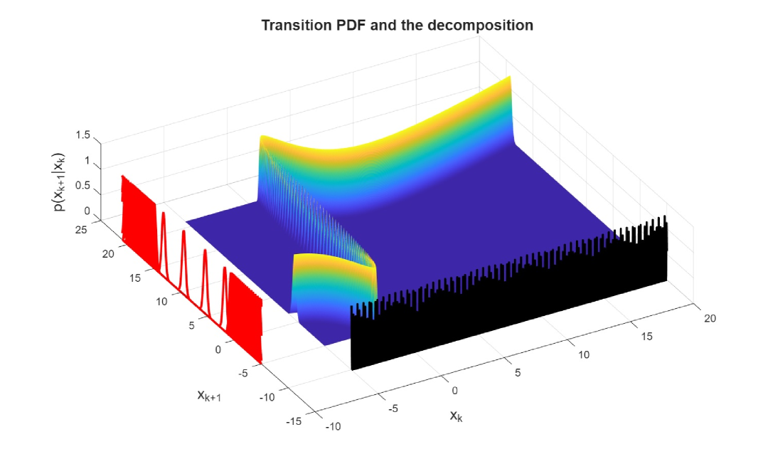
III-A Decomposition with filtered state grid
This decomposition described in [14] assumes the transition density (12) to be decomposed as
| (13) |
where functions and are given by Gaussian PDFs
| (14a) | ||||
| (14b) | ||||
The decomposition defines the fixed structure of the predictive PDF through setting parameters . The decomposition is illustrated in Figure 1 for a scalar state transition density
| (15) |
(for ) appearing in the highly nonlinear univariate nonstationary Gaussian model (UNGM) problem.
III-A1 Calculation of the parameters
The parameters , and the weights are calculated to minimize the squared error between the transition PDF and its approximation (13)
| (16) |
The reason for choosing the integral of a squared difference between the transition PDF and its approximation is the fact that for the Gaussian transition PDF (12) and the approximation (13), some terms can be integrated analytically. The large number of parameters makes the minimization of (16) intractable. Hence, some parameters are prescribed by the user, and the optimization is performed only over a few.
First, the number of terms and the location parameters are selected to achieve good approximation of (12) in the non-negligible support of the posterior . Second, the location parameters are calculated as
| (17) |
Third, covariances are set as due to (12). Fourth, to respect the shape of the function at the location , the covariance is set to be proportional to
| (18) |
where stands for the transpose of the inverse of . The proportionality factor denoted as is common for all . Its value is obtained by minimizing (16). Finally, the weights are set as
| (19) |
so that
| (20) |
The proportionality factor denoted as is common for all . Its value is obtained by minimizing (16). Hence, the criterion is minimized w.r.t. the proportionality factors and both being scalars.
III-A2 Possible generalization
When the function is time-varying, it may be necessary to recompute the decomposition for each time instant. In a special case, when the time instant acts in an additive way such as , where , the decomposition may be pre-computed only for a single time instant (e.g., ) and then shifted in direction of by .
The generalization to higher dimensions is straightforward. The number of location parameters may grow exponentially with the state dimension . Optimization of the criterion (16) to obtain the covariance matrices and the weights may be difficult but an approach similar to (18) and (19) may be used. The decomposition can also be designed for the non-Gaussian transition PDF.
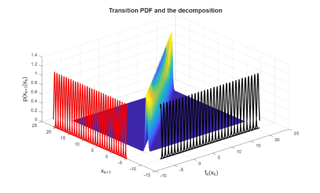
III-B Decomposition with predicted state grid
This decomposition assumes the transition density (12) decomposed as
| (21) |
where functions and are given by Gaussian PDF
| (22a) | ||||
| (22b) | ||||
The decomposition (21) was proposed in [16] to address the solution to the CKE for the PMF. The decomposition defines the fixed structure of the predictive PDF through parameters , and the weights . The decomposition is illustrated in Figure 2 for (15). Note that compared to the illustration in Figure 1, the axis-aligned grid is defined over the space of and rather than and , which is the case of FSG.
III-B1 Calculation of the parameters
The parameters are also obtained by an optimization process [16]. The number of terms and the locations are selected so that the approximation is good on the non-negligible support of the prior . The locations and are usually equal , and variances and are usually fixed and identical. They only depend on how dense the locations are. For optimal parameter values, the grid can easily be redefined over a hyper-rectangular region of arbitrary size.
III-B2 Possible generalization
The decomposition with PSG (21) can be straightforwardly generalized to higher dimensions as demonstrated in [16]. Similarly to the decomposition with the FSG, the number of components grows exponentially with the dimension of the state . The decomposition can be calculated for other classes of transition PDF such as Student-t distributed PDF [16]. Time-varying function in (1a) does not affect the decomposition since the decomposition is computed in the space of and as illustrated in Figure 2. Also, time-varying parameters of the transition PDF may not complicate the application of the decomposition since, for example, of Gaussian PDF, the decomposition was calculated for standard Gaussian distribution and the parameters and can easily be adapted for arbitrary covariance matrix.
IV GMFs with transition PDF decompositions
IV-A \Acgmf with transition PDF decomposition and FSG
The algorithm denoted as GMF-FSGD can be described using Algorithm 1.
Step 1 (initialization): Assume a posterior PDF
| (23a) | |||
| Step 2 (time update): Given the support of the posterior, select the parameters , , and weight . Calculate the CKE as | |||
| (23b) | |||
| which can be rewritten as | |||
| (23c) | |||
| where | |||
| (23d) | |||
| Then, the predictive PDF is of the form | |||
| (23e) | |||
| with and . | |||
Step 3 (measurement update): Update each parameter of using standard equations for GMF.
Note that for the transition PDF decomposition with FSG, no approximation is used when calculating the CKE since the function is a Gaussian PDF in . The prediction PDF in (23e) demonstrates that its structure is defined by the user through the locations .
IV-B \Acgmf with transition PDF decomposition and PSG
The algorithm denoted as GMF-PSGD can be described using Algorithm 2.
Step 1 (initialization): Assume a posterior PDF
| (24a) | |||
| Step 2 (time update): Given the support of the posterior, select the parameters , , and the weights . Calculate the CKE as | |||
| (24b) | |||
| which can be rewritten as | |||
| (24c) | |||
| where | |||
| (24d) | |||
| Then, the predictive PDF is of the form | |||
| (24e) | |||
| with . | |||
Step 3 (measurement update): Update each parameter of using standard equations for GMF.
For generally nonlinear , the integral in (24d) has to be evaluated approximately. The approximation error should be small since both variances and are small and the effect of the nonlinearity is thus limited. They are also identical by design, so the calculations can be simple.
IV-C Theoretical comparison of GMF-FSGD and GMF-PSGD
Both algorithms are based on a decomposition of the transition PDF, and their application for a state estimation problem must involve an offline stage, where the decomposition is pre-calculated. The comparison thus concentrates on both aspects: the offline precomputation stage and the algorithm application for online state estimation. Both grids are defined as axis-aligned. While FSG is defined over the space given by and , the PSG is defined over the space defined by and .
For the FSG, the offline stage involves the specification of a grid in the domain of . The grid has to cover the region where the state is expected to lie for . Defining the region may be challenging, and for real-world problems, one needs to run a simple filter first to provide a rough state estimate to determine the region. The size of the region substantially affects the number of terms of the decomposition. The online state estimation does not necessarily use all the terms of the decomposition (precomputed for all time instants) but rather a subset of terms relevant to the current state estimate . As mentioned above, the time-dependency of the function in (1a) may complicate the decomposition precalculation further.
All the difficulties of FSG stem from the definition of the grid over the space given by and . Since the PSG is defined over the space defined by and , it is only the process noise distribution that affects the PSG. Moreover, even if the distribution parameters vary in time, this dependency may not complicate the PSG computation. An example is the Gaussian with a time-varying mean or covariance matrix, where the PSG can be precomputed for a standard Gaussian distribution and then shifted and scaled to align with .
From the offline stage calculation point of view, the FSG is more difficult to calculate than the PSG. Both grids are usually specified to be equidistant, which for the FSG may lead to limited approximation accuracy in areas when small changes to correspond to big changes in . This is illustrated in Figure 3, where the UNGM transition PDF is decomposed for both FSG and PSG.
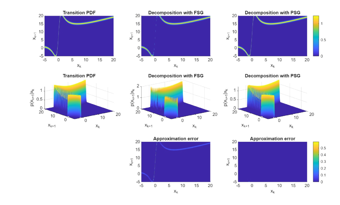
The disadvantage of the decomposition with FSG is compensated in the online state estimation, where due to the function (14b) being Gaussian PDF in , the integration in (23d) can be evaluated analytically. The GMF-PSGD has to calculate the corresponding integral (24d) numerically as the function in (22b) is a Gaussian PDF in rather in . The numerical approximation used for the evaluation may be a simple one, e.g., the cubature rule, which is computationally cheap and leads to satisfactory results since both PDFs, which product appears in the integral, have similar covariance matrices.
V Numerical illustration
Consider the UNGM [17], which is strongly nonlinear and often used as a benchmark problem. Its transition PDF is given in (15) and measurement PDF
| (25) |
In this paper, we consider the process and measurement noise variances and , respectively, and the initial condition being Gaussian with zero mean and variance .
The state of the UNGM was estimated by
-
•
GMF-FSGD with equidistant locations with distance between neighborhood locations ,
-
•
GMF-PSGD with the decomposition parameters computed in [16] with rank 40,
-
•
PMF [18] with grid points,
-
•
PF with the importance density given by the transition PDF, multinomial resampling at each time instant, and samples.
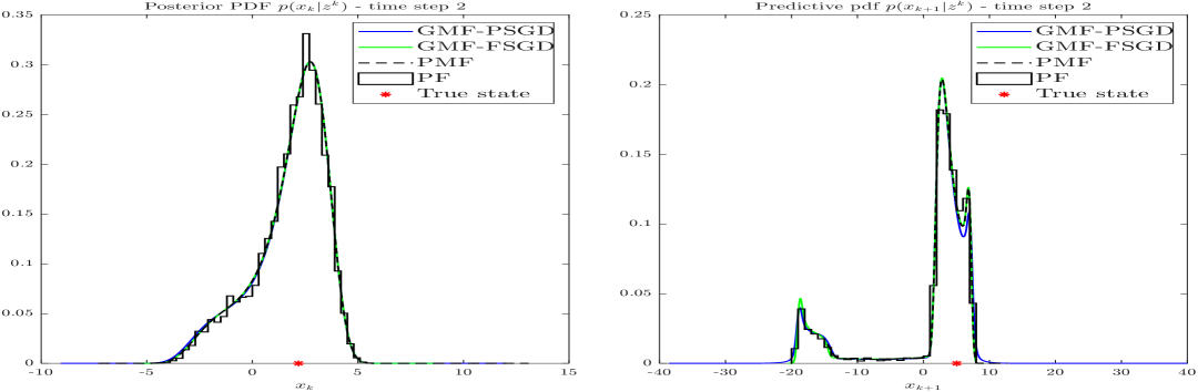
First, the predictive and filtering PDFs for are shown in Figure 4 to illustrate the capability of the proposed filters to produce a good approximation of complex-shaped PDFs.
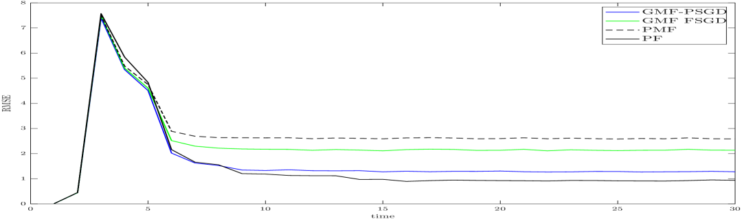
Then, the root mean-squared error (RMSE)
| (26) |
based on Monte Carlo (MC) simulations was computed with being the true state at -th MC simulation and being its filtering estimate. It is shown in Figure 5, from which it follows that for the above-mentioned parameters, the best RMSE performance has the PF. The GMF-PSGD performs better than the GMF-FSGD, which is probably given by the fact that the decomposition with the FSG has worse approximation quality in some regions compared to the decomposition with the PSG.
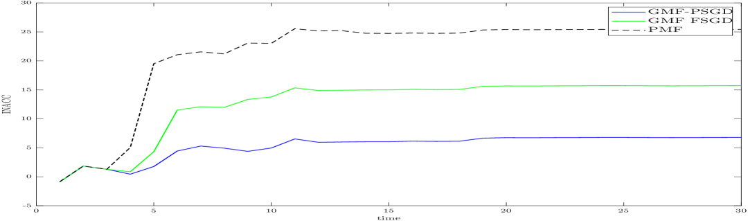
Since the RMSE only evaluates the quality of point estimates, the proposed methods are also assessed based on the quality of the posterior PDF. The performance was analyzed in terms of Kullback-Leibler divergence (KLD) between the posterior PDF produced by the PF with samples representing the true posterior and the posterior PDFs produced by GMF-PSGD, GMF-FSGD, and PMF. The posterior PDF of the PF is given as
| (27) |
where is the Dirac-delta function and is the -th sample. The KLD defined as
| (28) |
consists of Shanon differential entropy (SDE) and inaccuracy (INACC) [19]. The discrepancy between the PDFs is captured by the inaccuracy only; hence, it will be used for the comparison. The inaccuracy averaged over the MC simulations is depicted in Figure 6. From the figure, it follows that superior performance is achieved by the GMF-PSGD while the PMF does not perform well.
The computational time of the algorithms is compared in terms of the time of the filter’s single step, given in Table I
| GMF-PSGD | GMF-FSGD | PF | PMF | |
| Time [ms] | 0.78 | 1.96 | 4.29 | 6.09 |
The results indicate that the GMF-PSGD algorithm is computationally cheaper than GMF-FSGD. This was not expected since GMF-PSGD uses numerical integration while GMF-FSGD uses analytical integration in the online run. The reason for this is the number of terms, which was higher for GMF-FSGD (286 GM terms on average) than for GMF-PSGD (80 GM terms on average). The difference is caused by different approximations and sizes of the approximation regions used by the algorithms. It shall be noted that all the above results depend on the specification of the filter parameters, such as the number of grid points, samples, and GM terms in the transition PDF decomposition. Comparing the performance of the filters is challenging due to differing parametrization. Therefore, the purpose of the numerical example is to showcase the competitiveness of the proposed algorithms when compared with the representative Bayesian filtering algorithms.
VI Conclusion
The paper proposed practical Gaussian mixture filters that do not rely on local component processing and do not suffer from component explosion. The key idea of these global filters is the offline decomposition of a given transition density into a mixture of axis-aligned Gaussian components. These decompositions automatically maintain a predefined number of posterior components without requiring explicit component reduction. Two types of decompositions are derived that differ in the definition of the coordinate axes. While the first decomposition uses and as axes, the second one uses and . The first decomposition has complex offline processing and requires the specification of an approximation domain. However, for Gaussian and Gaussian mixture posteriors, the prediction step can then be performed online in closed form. The second decomposition is simple to perform and does not require a predefined approximation domain but requires numerical integration (done by the unscented transform). Both decompositions allow an adjustable trade-off between the computational load during the online prediction step and the estimation quality achieved. Numerical simulations with a highly nonlinear univariate nonstationary Gaussian model (UNGM) problem demonstrated that the proposed algorithms are competitive compared to the state-of-the-art Bayesian filtering methods in terms of both point estimate quality and posterior PDF quality.
Future work will focus on the calculation of more efficient decompositions for GMF-FSGD and its generalization to higher dimensions, as GMF-PSGD can easily be extended to mid dimensions (approx. ten state elements).
References
- [1] I. Arasaratnam and S. Haykin, “Cubature Kalman filters,” IEEE Transactions on Automatic Control, vol. 54, no. 6, pp. 1254–1269, 2009.
- [2] J. Duník, O. Straka, and M. Šimandl, “Stochastic integration filter,” IEEE Transactions on Automatic Control, vol. 58, no. 6, pp. 1561–1566, 2013.
- [3] M. Šimandl, J. Královec, and T. Söderström, “Advanced point-mass method for nonlinear state estimation,” Automatica, vol. 42, no. 7, pp. 1133–1145, 2006.
- [4] B. Ristic, S. Arulampalam, and N. Gordon, Beyond the Kalman Filter: Particle Filters for Tracking Applications. Artech House, 2003.
- [5] H. Sorenson and D. Alspach, “Recursive Bayesian Estimation Using Gaussian Sums,” Automatica, vol. 7, no. 4, pp. 465–479, 1971.
- [6] K. Ito and K. Xiong, “Gaussian Filters for Nonlinear Filtering Problems,” IEEE Transactions on Automatic Control, vol. 45, no. 5, pp. 910–927, 2000.
- [7] D. Durant, U. D. Hanebeck, , and R. Zanetti, “Good things come to those who weight! improving gaussian mixture weights for cislunar debris tracking,” in Proceedings of the AAS/AIAA Space Flight Mechanics Meeting, Kaua’i, Hawaii, no. 25, Kaua’i, Hawaii, January 2025, p. 309.
- [8] J. Kotecha and P. Djuric, “Gaussian Sum Particle Filtering,” IEEE Transactions on Signal Processing, vol. 51, no. 10, pp. 2602–2612, 2003.
- [9] J. H. Kotecha and P. M. Djuric, “Gaussian particle filtering,” IEEE Transactions on Signal Processing, vol. 51, no. 10, pp. 2592–2601, 2003.
- [10] U. D. Hanebeck and O. Feiermann, “Progressive bayesian estimation for nonlinear discrete-time systems: The filter step for scalar measurements and multidimensional states,” in Proceedings of the 2003 IEEE Conference on Decision and Control (CDC 2003), Maui, Hawaii, USA, December 2003, p. 5366–5371.
- [11] D. Frisch and U. D. Hanebeck, “Gaussian mixture particle filter step based on method of moments,” in Proceedings of the 27th International Conference on Information Fusion (FUSION 2024), Venice, Italy, July 2024.
- [12] U. D. Hanebeck, D. Frisch, and D. Prossel, “Closed-form information-theoretic roughness measures for mixture densities,” in Proceedings of the 2024 American Control Conference (ACC 2024), Toronto, Canada, July 2024.
- [13] A. G. Wills, J. Hendriks, C. Renton, and B. Ninness, “A Numerically Robust Bayesian Filtering Algorithm for Gaussian Mixture Models,” in IFAC-PapersOnLine, ser. 12th IFAC Symposium on Nonlinear Control Systems NOLCOS 2022, vol. 56, 2023, pp. 67–72.
- [14] M. Huber, D. Brunn, and U. D. Hanebeck, “Closed-form prediction of nonlinear dynamic systems by means of gaussian mixture approximation of the transition density,” in Proceedings of the 2006 IEEE International Conference on Multisensor Fusion and Integration for Intelligent Systems (MFI 2006), Heidelberg, Germany, September 2006, p. 98–103.
- [15] Y. Bar-Shalom, X. R. Li, and T. Kirubarajan, Estimation with Applications to Tracking and Navigation: Theory Algorithms and Software. John Wiley & Sons, 2001.
- [16] P. Tichavský, O. Straka, and J. Duník, “Grid-based bayesian filters with functional decomposition of transient density,” IEEE Transactions on Signal Processing, vol. 71, pp. 92–104, 2023.
- [17] N. Gordon, D. Salmond, and A. F. M. Smith, “Novel approach to nonlinear/ non-gaussian bayesian state estimation,” IEE Proceedings-F, vol. 140, pp. 107–113, 1993.
- [18] M. Simandl, J. Kralovec, and P. Tichavsky, “Filtering, predictive and smoothing cramér-rao bounds for discrete-time nonlinear dynamic filters,” Automatica, vol. 37, no. 11, pp. 1703–1716, 2001.
- [19] R. Kulhavy, Recursive Nonlinear Estimation. Springer, 1996, vol. 216.