Scaling Quantum Simulation-Based Optimization: Demonstrating Efficient Power Grid Management with Deep QAOA Circuits

Abstract

Quantum Simulation-based Optimization (QuSO) is a recently proposed class of optimization problems that entails industrially relevant problems characterized by cost functions or constraints that depend on summary statistic information about the simulation of a physical system or process. This work extends initial theoretical results that proved an up-to-exponential speedup for the simulation component of the QAOA-based QuSO solver proposed by Stein et al. for the unit commitment problem [1] by an empirical evaluation of the optimization component using a standard benchmark dataset, the IEEE 57-bus system. Exploiting clever classical pre-computation, we develop a very efficient classical quantum circuit simulation that bypasses costly ancillary qubit requirements by the original algorithm, allowing for large-scale experiments. Utilizing more than 1000 QAOA layers and up to 20 qubits, our experiments complete a proof of concept implementation for the proposed QuSO solver, showing that it can achieve both highly competitive performance and efficiency in its optimization component compared to a standard classical baseline, i.e., simulated annealing.

I Introduction

Quantum computing has the potential to disrupt the domains of optimization and simulation, offering up to exponential speedups in both areas [2, 3, 4, 5, 6, 7, 8, 9, 10]. Quantum Simulation-based Optimization (QuSO) is a newly proposed class of optimization problems that involve the execution of complex simulations, such as solving Partial Differential Equations (PDEs) or high-dimensional systems of linear equations, to determine the cost of a potential solution or ensure the satisfaction of constraints [1]. A simple example of such a problem can take the form of

$$\operatorname*{arg\,min}_{x\in\mathbb{B}^{n}}f(x,y)\quad\textnormal{s.t.}\quad Ay=b(x),$$ (1)

for a freely choosable $y\in\mathbb{R}^{m}$, given fixed $b:x\mapsto\mathbb{R}^{m}$, and given fixed $A\in\mathbb{R}^{m\times m}$ invertible. For this example, the equality constraint $Ay=b(x)$ would constitute a simulation problem and $f:(x,y)\mapsto\mathbb{R}$ may denote an NP-hard, polynomial objective function. As $m$ is often very large, the predominant classical approach to solve such problems is iterative search, i.e., (1) probing an initial solution $x\in\mathbb{B}^{n}$, (2) solving the system of linear equations $Ay=b(x)$ to yield the value of $y$ allowing for (3), the computation of the objective value $f(x,y)$ and finally (4), trying to find better solutions by repeating these steps with a newly guessed solution candidate [11].

These types of problems arise in many areas of application and research such as pharmaceutical development [12] or aircraft design [13], where intricate physical models must be optimized within resource or cost constraints. The key feature of QuSO problems is that the information required from the result of the simulation must be easily extractable, i.e., it must take the form of summary statistic information (cf. Ref. [2] and Definition 2). This makes it feasible to use quantum algorithms to perform the simulation component of the problem while not suffering from the well-known output problem. This specific requirement distinguishes QuSO from traditional simulation-based optimization and allows it to achieve significant quantum speedups.

In Ref. [1], Stein et al. proposed a combination of the Quantum Approximate Optimization Algorithm (QAOA) to solve the optimization component with the Quantum Singular Value Transformation (QSVT) to compute the simulation outcome. They further demonstrated the potential for up-to-exponential quantum advantage in the context of the unit commitment problem, which is essentially the problem of optimizing the energy production costs by choosing which power generators to activate for a given power demand of all loads in a power grid. There, a simulation task arises inside the power transmission costs, which are determined by how much power flows over which transmission line, requiring a simulation of the overall power flow. For this provably QuSO-type problem, the proposed algorithm was shown to reduce the computational complexity of the simulation component to $\tilde{\mathcal{O}}(\log(N)\kappa s)$, compared to the classical $\tilde{\mathcal{O}}(N\sqrt{\kappa}s)$ complexity achieved by the conjugate gradient method [14], where $N$ denotes the problem size, $\kappa$ the condition number of the system of linear equations (SLE) to be solved (which is usually linear in $N$ for real-world applications) and $s$ the sparsity of this SLE. Furthermore, for certain topologies–specifically expander graphs–their approach can even achieve provably exponential quantum speedups in $N$, as the condition number $\kappa$ is constant for such graphs by reducing the runtime complexity from $\tilde{\mathcal{O}}(Ns)$ to $\tilde{\mathcal{O}}(Ns)$  [1]. This theoretical advantage motivates further exploration into the practical applicability of the proposed QuSO solver addressing industrially relevant problems on realistic datasets.

The main contribution of this paper is to investigate the performance of the optimization component of the QuSO solver proposed in Ref. [1], as in that reference, only the simulation component was explored for possible quantum advantages. More concretely, we develop an efficient numerical simulation of the quantum algorithm and conduct an empirical evaluation of the proposed QuSO solver against a classical state-of-the-art approach on the IEEE 57-bus system, a standard dataset in power systems research [15]. The classical circuit simulation algorithm is implemented by cleverly simplifying the proposed QuSO solver to a diagonalized QAOA using extensive classical precomputation of quantum subroutines based on ideas of [16]. Our results demonstrate that the quantum approach achieves competitive performance, continuously displaying approximation ratios above 95% for problem instances entailing up to 20 qubits.

The remainder of this paper is structured as follows. We first outline the necessary preliminaries on the employed QuSO solver in Section II. We then introduce the utilized problem formulation of the unit commitment problem and present our approach to solving it using a simplified version of the originally proposed QuSO solver for classical circuit simulation in Section III. The experimental setup including baselines and datasets is outlined in Section IV. The results of the empirical benchmark study are described in Section V and discussed in Section VI. Finally, we conclude our findings in Section VII.

II Quantum Simulation Based Optimization

This section outlines a formal definition of QuSO according to Ref. [1], foundational concepts of quantum optimization via the Quantum Approximate Optimization Algorithm (QAOA), as well as the employed QuSO solver.

II-A Quantum Simulation-based Optimization

QuSO is defined as a subset of Mixed-Integer Nonlinear Programming (MINLP), which represents a very broad class of optimization problems. For simplicity, we focus solely on minimization problems in the remainder of this paper.

Definition 1.

A Mixed-Integer Nonlinear Programming (MINLP) problem is about minimizing a function $f(x)$ subject to constraints $c_{j}(x)\leq 0$ for all $j\in[K]$, with continuous bounds $x_{i}\in[l_{i},u_{i}]\subset\mathbb{R}$ and integer constraints $x_{i}\in\mathbb{Z}$ for certain indices $i\in I\subseteq[N]$, where $f:\mathbb{R}^{N}\rightarrow\mathbb{R}$ and $c:\mathbb{R}^{N}\rightarrow\mathbb{R}^{K}$ are continuous functions.

As QuSO is defined based on the concept of summary statistic information, which we now define formally:

Definition 2 (Summary Statistic Information).

Given an oracle $O$ that prepares an $n$-qubit quantum state $\ket{\psi}=O\ket{0}^{\otimes n}$, summary statistic information refers to a binary-encoded output from a quantum algorithm that relies on $\ket{\psi}$, given access to $O$.[17]

Definition 3 (Quantum Simulation-based Optimization (QuSO)).

A QuSO problem is a MINLP problem where the objective function and/or constraints depend on the summary statistic result of a simulation problem, as in:

$$\text{minimize}_{x} f(x,u(s(x)))$$

subject to $$c_{j}(x,u(s(x)))\leq 0,\;\forall j\in[K],$$

$$x_{i}\in[l_{i},u_{i}]\subset\mathbb{R},$$

$$x_{i}\in\mathbb{Z},\;\forall i\in I\subseteq[N],$$

where $f:\mathbb{R}^{N}\times\{0,1\}^{m}\rightarrow\mathbb{R}$ and $c:\mathbb{R}^{N}\times\{0,1\}^{m}\rightarrow\mathbb{R}^{K}$ are continuous functions, $s:\mathbb{R}^{N}\rightarrow\mathbb{R}^{M}$ represents a simulation problem, and $u:\mathbb{R}^{M}\rightarrow\{0,1\}^{m}$ extracts summary statistic information from $s(x)$.

QuSO encompasses all simulation-based optimization problems that can potentially benefit from quantum speedup in the simulation component. While this paper focuses on simulations that can be natively expressed as a system of linear equations, QuSO also includes problems with non-linear simulations problems (e.g., Navier-Stokes equations [18]). QuSO’s main feature is its requirement that information from the simulation results be extractable, which if can be done reasonably efficiently implies that obtaining summary statistics does not negate any quantum speedup from the simulation process.

II-B The Quantum Approximate Optimization Algorithm

Being the basis of the employed QuSO solver, we now outline the Quantum Approximate Optimization Algorithm (QAOA), which is an approximate version of the Quantum Adiabatic Algorithm (QAA) [19], leveraging the Adiabatic Theorem [20] to find (approximate) solutions of unconstrained combinatorial optimization problems. For a binary objective function $f:\{0,1\}^{n}\rightarrow\mathbb{R}$, QAOA operates as follows [21]:

1. Map objective values to the energy levels of a Hamiltonian $H_{C}=\sum_{x}f(x)\ket{x}\!\bra{x}$.

2. Initialize the system in the ground state of a Hamiltonian, e.g., $H_{M}=-\sum_{i=1}^{n}\sigma_{i}^{x}$ and ground state $\ket{+}^{\otimes n}$.

3. Simulate the time evolution $\exp(-i\int_{0}^{T}H_{s}(t)\,dt)$, where $H_{s}(t)=(1-s(t))H_{M}+s(t)H_{C}$ guides the adiabatic transition, with $s:[0,T]\rightarrow[0,1]$ transitioning from 0 to 1.

4. Measure the final state $\ket{\psi}$ and map it back to a solution for $f$.

To implement this time evolution on gate-based quantum computers, the QAOA discretizes the continuous Hamiltonian into $p$ segments $H_{s}(1/T),\dots,H_{s}(T)$ and applies a first-order Suzuki-Trotter approximation. This yields the unitary operator:

$$U(\beta,\gamma)=U_{M}(\beta_{p})U_{C}(\gamma_{p})\ldots U_{M}(\beta_{1})U_{C}(\gamma_{1}),$$ (2)

where $\beta_{i}$ and $\gamma_{i}$ are introduced as variables that control the evolution rate, and $U_{M}(\beta_{i})=e^{-i\beta_{i}H_{M}}$, $U_{C}(\gamma_{i})=e^{-i\gamma_{i}H_{C}}$. As $p\rightarrow\infty$, $U(\beta,\gamma)$ approximates the adiabatic evolution more accurately. Efficient training procedures and initializations for the parameters have been established in related work such as Refs. [22, 23].

II-C QuSO solving

We now introduce the overall setup of the proposed QuSO solver as defined in Theorem 1.

Theorem 1 (QuSO Solver Architecture [1, Thm. 10]).

The circuit displayed in Figure 1 implements a quantum algorithm for solving a QuSO problem of the form $\operatorname*{arg\,min}_{x}u(s(x))$ given an oracle $\textnormal{QSim}\ket{x}\ket{0}^{\otimes m}=\ket{x}\ket{u(s(x))}$.

[column sep=6.5pt, row sep=10pt] $\ket{0}^{\otimes n}$ U_S[1,steps=1,style=inner xsep=0pt, fill=green!20,background,label style=label position=above,anchor=south, yshift=-0.8mm]State Prep. [4][1.8cm]QSim[1]$x$[1]$x$[4,steps=4,style=inner xsep=0pt, fill=blue!20,background,label style=label position=above,anchor=south, yshift=-0.8mm]Cost-Unitary $U_{C}(\gamma_{1})$ [4]QSim^† [-0.2cm] U_M(β_1)[1,steps=1,style=inner xsep=0pt, fill=red!20,background,label style=label position=above,anchor=south, yshift=-0.8mm]Mixer-Unitary $U_{M}(\beta_{1})$  …  U_C(γ_p) U_M(β_p) [4][1.8cm]QSim[1]$x$[1]$x$[4,steps=1,style=inner xsep=0pt, fill=teal!20,background,label style=label position=above,anchor=south, yshift=-0.8mm]Cost computation
n [3]$\ket{0}^{\otimes m}$n [3]$0$[3]$u(s(x))$ P(-γ_1 2^-1) n n n n n [3,brackets=right]$\ket{0}^{\otimes m}$n [3]$0$[3]$u(s(x))$
n . . . n n . . . n n n n n n n n n n . . . n
n n n P(-γ_1 2^-m) n n n n n n

Figure 1: Quantum circuit addressing a QuSO problem of the form $\arg\min_{x}f(x)=u(s(x))$, as outlined in Theorem 1. A possible implementation of QSim is detailed in Ref. [1, Fig. 9]. The $\quantikz\ground{}$ symbol indicates ancillary qubits initialized in the $\ket{0}$ state, which can be reused for subsequent calculations. This circuit is taken from Ref. [1].

If the simulation component of the QuSO problem takes the form of a system of linear equations (as assumed for the rest of this paper and applicable to the problem of interest), exponential speedups are possible if the following conditions are met [1]:

1. The SLE is sparse and well-conditioned.

2. The dependency of the SLE on decision variables allows efficient input to a quantum linear system solver.

3. Summary statistic information from the SLE solution can be extracted efficiently.

For the sake of brevity, we refer the reader to Ref. [1] for any further details on the simulation component, as that section of the algorithm will not be part of more thorough consideration within this manuscript, as we concentrate on classical simulations of the algorithm, which can exploit precomputation of the diagonal cost unitary without any additional ancillary qubits needed (cf. Section III-B).

III Benchmarking Methodology

In this section, we define the specific version of the unit commitment problem addressed in this paper and propose a simplified implementation using extensive classical precomputation combined with a diagonalized form of the QAOA.

III-A The Unit Commitment Problem

The unit commitment problem is a MINLP-type optimization problem that determines which power generators should operate within a power grid to meet a given estimated load at the lowest possible cost. The associated simulation problem, known as the power flow problem, involves calculating the power flow through each transmission line, $\vec{\rho}$, based on the power input and output at each node (referred to as buses) in the power grid, $p_{i}$. The costs of this power flow problem can be expressed as $|\langle\vec{c},\vec{\rho}_{x}\rangle|$, where $\vec{c}$ represents the linear cost factor for transmitting power over each transmission line. Although the unit commitment problem includes many additional cost factors and constraints in practical settings (which can, in principle, be incorporated into the proposed QuSO solver [1]), this paper focuses on a simplified version to serve as a proof of concept. Specifically, we investigate a widely used linear approximation of AC power flow: the DC power flow approximation as detailed in Definition 4 taken from Ref. [1].

Definition 4 (Unit Commitment Problem (UCP)).

Given a power grid in form of a graph $\mathcal{G}=(V,E)$ of its transmission lines weighted by their susceptances $\vec{b}_{ij}\in\mathbb{R}$, $V=\left\{1,...,N\right\}$, a fixed value how much power $\vec{p}_{i}\in\mathbb{R}$ is generated or consumed (where, respectively $\vec{p}_{i}\in\mathbb{R}_{+}$, or $\vec{p}_{i}\in\mathbb{R}_{-}$) by each generator $i\in G=\left\{1,...,M\right\}\subset V$ and load $i\in L\coloneqq V\setminus G$, a reference bus $r\in V$ (wlog. $r=N$), as well as fixed values for the linear cost factor of using each transmission line $\vec{c}_{ij}\in\mathbb{R}$, then we define the problem of power flow focused unit commitment by

$$\operatorname*{arg\,min}_{x}\langle\vec{c},|\vec{\rho}_{x}|\rangle\quad\textnormal{s.t.}\quad\sum_{i}\vec{p}_{x}\approx 0,$$ (3)

i.e., optimizing which generators $G_{x}\coloneqq\left\{i\in G:x_{i}=1\right\}$ should be operating to minimize the overall power transmission costs using the decision variables $x\in\left\{0,1\right\}^{M}$ while the net power input is roughly equal to the net power output. Here, $\vec{\rho}_{x}\coloneqq B^{\prime}\Pi\mathord{\text{$\mkern-2.0mu\raisebox{-3.65973pt}[0.0pt][0.0pt]{$\mathchar 22\relax$}\mkern-8.0mu\mathcal{B}$}}^{-1}\vec{\mathord{\text{$\mkern-2.0mu\raisebox{-6.45831pt}[0.0pt][0.0pt]{$\mathchar 22\relax$}\mkern-7.0mup$}}}_{x}$ denotes the power flowing over all transmission lines, where $\vec{\mathord{\text{$\mkern-2.0mu\raisebox{-6.45831pt}[0.0pt][0.0pt]{$\mathchar 22\relax$}\mkern-7.0mup$}}}_{x}$ is the reduced form of the power in-/output vector $\vec{p}_{x}$ (i.e., $\vec{p}_{x}$ without its $r$-th entry), which is defined as either $\vec{p}_{i}$ iff $i\in L$ or $x_{i}\vec{p}_{i}$ iff $i\in G$, further, $\mathcal{B}$ is defined as the Laplacian matrix of $\mathcal{G}$ with weights $\vec{b}_{ij}$ and $\mathord{\text{$\mkern-2.0mu\raisebox{-3.65973pt}[0.0pt][0.0pt]{$\mathchar 22\relax$}\mkern-8.0mu\mathcal{B}$}}\coloneqq\mathcal{B}\left[r\right]$ (i.e., the matrix that results when the $i$-th row and $i$-th column are removed from $\mathcal{B}$, where $i\in\left[N\right]$). Finally, $\Pi$ denotes the projection matrix mapping $\vec{\mathord{\text{$\mkern-2.0mu\raisebox{-4.09024pt}[0.0pt][0.0pt]{$\mathchar 22\relax$}\mkern-5.1mu\theta$}}}\coloneqq\mathord{\text{$\mkern-2.0mu\raisebox{-3.65973pt}[0.0pt][0.0pt]{$\mathchar 22\relax$}\mkern-8.0mu\mathcal{B}$}}^{-1}\vec{\mathord{\text{$\mkern-2.0mu\raisebox{-6.45831pt}[0.0pt][0.0pt]{$\mathchar 22\relax$}\mkern-7.0mup$}}}_{x}$ onto $\vec{\theta}^{\prime}\coloneqq(\vec{\theta}_{1},...,\vec{\theta}_{1},\vec{\theta}_{2},...,\vec{\theta}_{2},...,\vec{\theta}_{N},...,\vec{\theta}_{N})$ where each $\vec{\theta}_{i}\coloneqq\vec{\mathord{\text{$\mkern-2.0mu\raisebox{-4.09024pt}[0.0pt][0.0pt]{$\mathchar 22\relax$}\mkern-5.1mu\theta$}}}_{i}\;\forall i\neq r$ appears exactly $d_{i}\coloneqq\left|\left\{j\in V:(i,j)\in E\right\}\right|$ often and $\vec{\theta}_{r}=0$ for the chosen reference bus. Lastly, $B^{\prime}$ takes the form of an $|E|\times|E|$ dimensional matrix with diagonal entries $(\vec{b}_{1e(1,1)},...,\vec{b}_{1e(1,d_{i})},...,\vec{b}_{Ne(N,1)},...,\vec{b}_{Ne(N,d_{N})})$, where a given function $e:V\times\mathbb{N}\rightarrow V,v,j\mapsto w$ yields $w\in V$, i.e., the $j$-th neighbor of node $i$, and off-diagonal entries $-\vec{b}_{ie(i,k)}$ for the $(k+\sum_{\iota=1}^{i-1}\iota d_{\iota})$-th row.

As shown in Ref. [1], the associated cost function can be efficiently computed within the QuSO QSim framework, as restated in the following theorem.

Theorem 2 (QSim implementation for the UCP [1, Thm. 13]).

If $s(x)$ takes the form of a linear system of equations and $u(x)$ takes the form of an inner product as in Definition 4, we can implement the corresponding oracle $\textnormal{QSim}\ket{x}\ket{0}^{\otimes m}=\ket{x}\ket{u(s(x))}$ within a quantum circuit of depth $\tilde{\mathcal{O}}(\operatorname{polylog}(N)\kappa^{*}s/\varepsilon\delta)$ using $\tilde{\mathcal{O}}(N^{2})$ ancillary qubits, where $\varepsilon$ denotes the accuracy of extracting the summary statistic solution, and $0<\delta<1$ the success probability of the algorithm.

III-B Quantum Circuit Implementation

As the circuit proposed in Theorem 1 has components that inherently rely on not yet realized fault-tolerant quantum computing (e.g., the QSVT), all evaluations must be performed using classical simulators. This allows for substantial simplifications of the required subroutines within the algorithm, as its most complex component–the cost unitary–can be precomputed classically resulting in a diagonal matrix with entries $\exp(-i\gamma_{i}u(s(x)))$ for all $x$. While this requires each possible solution to be computed individually hence increasing the computational complexity of the optimization algorithm exponentially, this step is crucial in reducing the number of qubits to the bare minimum, i.e., this approach only requires as many qubits as there are decision variables. As classical quantum circuit simulation is mostly bottlenecked with the number of available qubits, this allows us to test for the largest scale problems possible, which best indicate the eventual scaling of the proposed QuSO solver. For the concrete implementation, we utilize qulacs and employ the add_gate() function with the precomputed qulacs.gate.DiagonalMatrix to efficiently implement the cost unitary similar to the QAOA simulation approach proposed in Ref. [16].

The other components of the proposed algorithm (cf. Figure 1) consist only of the state preparation routine and the mixer unitary. As we use the standard $X$-Mixer, together with the $\ket{+}^{\otimes n}$ state as its corresponding ground state, we simply have $U_{S}=H^{\otimes n}$ and $U_{M}(\beta_{i})=e^{-i\beta_{i}X}$. The final step of cost computation displayed in Figure 1 is not simulated inside the quantum circuit, as it is unnecessary in our implementation, based on the fact that we already have precomputed each cost value for all solutions.

IV Experimental Setup

In this section, we introduce the hyperparameters for the classical baseline and our quantum approach, the dataset and the evaluation metrics.

IV-A Classical Baseline

As a classical baseline we use Simulated Annealing (SA) [24] as it is an iterative, gradient-free search algorithm that allows solving the simulation problem with specialized solvers like the conjugate gradient method as opposed to a MILP solver like CPLEX or Gurobi, for which the number of equality constraints becomes excessively large for high dimensional simulation problems.

The here employed version of Simulated Annealing begins with a (typically random) initial solution $x\in\mathcal{X}$ and conducts a local search. During this, it iteratively chooses a neighboring solution $x^{\prime}\in\mathcal{N}(x)$ at random in each step, where $\mathcal{N}(x)$ are the Hamming weight $1$ neighbors of $x$. If the new candidate $x^{\prime}$ improves the objective function, it is accepted unconditionally (i.e., $x\leftarrow x^{\prime}$). If $x^{\prime}$ has a worse objective value, it is accepted with probability $P(x,x^{\prime},T)\coloneqq e^{-\left|C(x)-C(x^{\prime})\right|/kT}$. Here, $k$ is a user-defined constant (we utilize the popular choice of it corresponding to the Boltzmann constant), and $T_{i}$ represents the temperature at iteration $i$, which is updated according to a predefined annealing schedule. We employ the commonly used geometric annealing schedule, where the temperature decreases exponentially according to $T_{i}\leftarrow\alpha T_{i-1}$, with initial temperature $T_{0}$ and decay parameter $\alpha\in(0,1)$ [25]. For our experiments, we explore a range of temperature iteration steps starting at $10$ and increasing to $80$ in steps of size $10$. The algorithm the returns the best solution identified over a specified maximum number of iterations and is repeated for a specific amount of times to ensure statistic relevance (for our experiments we use 10 samples). For simplicity and reproducibility, we adopt the SA implementation from [26].

Figure 2: This IEEE 57-bus test case represents a simple approximation of the American Electric Power system (in the U.S. Midwest) from the early 1960s [15]. The data were provided by I. Dabbagchi and converted into the IEEE Common Data Format by R. Christie at the University of Washington in August 1993 [27]. This bus test case system has 57 buses, 7 generators, and 42 loads.

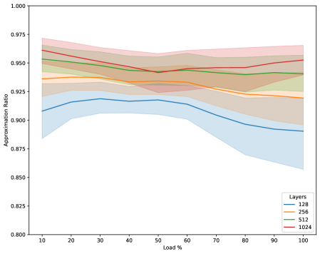
(a) QAOA solution quality for various circuit depths.

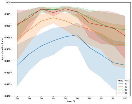
(b) SA solution quality for various numbers of temperature iterations.

Figure 3: Solution quality comparison between QAOA and SA showing the approximation ratio across all load percentages averaged over all qubits. The shaded area represents the 95% confidence interval.

IV-B Dataset

For the desired proof of concept evaluation, we choose the frequently employed IEEE 57-bus test case, which represents a simple approximation of the American Electric Power system from the early 1960s, shown in Figure 2. By assigning each node to be either a generator or a load, we slightly change the original dataset to allow for a smooth scaling of the size of the regarded problem instances, as each generator entails one binary decision variable. The assignment of nodes to either generators or loads was done using random sampling using a constant seed for reproducibility (in this case 15). The total generating capacity of the system is fixed at 1000 MW and evenly distributed among all generators. The total load of the system is varied from $10\%$ to $100\%$ of the total generating capacity in $10$% steps. This full coverage of possible load demands is selected to provide a complete picture of possible real-world scenarios and further has been shown to include a phase transition [28], which is crucial to include hard problem instances to ensure robust benchmarking (cf. [29]. The load of each individual node is sampled at random initially and then scaled across all nodes to match the total load of the system, using a constant seed (i.e., 15 in our implementation). The total generating capacity is based on the scale of the original values from the IEEE dataset.

IV-C Evaluation Metrics

The main metric used in this paper is the Approximation Ratio (AR) defined as $1-f(x)/f(x_{\textnormal{opt}})$ and therefore ranges from the worst possible solution quality $\max_{x}f(x)$ at value 0 to the optimal solution $f(x_{\textnormal{opt}})\coloneqq\min_{x}f(x)$ at value 1. To more easily calculate the approximation ratio we first rescale all the costs found with 3 to be between 0 and 1 using a min/max rescaling.

$$\textnormal{cost}\leftarrow\dfrac{f(x)-\min_{x}f(x)}{\max_{x}f(x)-\min_{x}f(x)}$$ (4)

The approximation ratio can then be simplified to:

$$AR(cost)=1-cost$$ (5)

The AR is thus bound between 1.0 and 0.0, with 1.0 corresponding to the optimal solution and 0.0 corresponding to the worst possible solution.

The other employed main metric is Time to Solution (TTS), which we defined as the minimum number of computing steps $s$ needed in order to yield a solution with an approximation ratio $P_{s}$ exceeding a predefined threshold (e.g., $95\%$) with a probability of at least 99% (cf. Ref. [29]). For the sake of simplicity we define the number of computational steps for the QAOA as its layer complexity (as the depth of each layer has been shown to be logarithmic in Ref. [1]) and the number of temperature iterations for the employed classical baseline Simulated Annealing. The TTS metric is used to find the most efficient algorithm configuration that is able to generate results that exceed the chosen threshold.

$$TTS=\min_{s}s\cdot\left(\frac{\log(0.01)}{\log(1.0-P_{s})}+1\right)$$ (6)

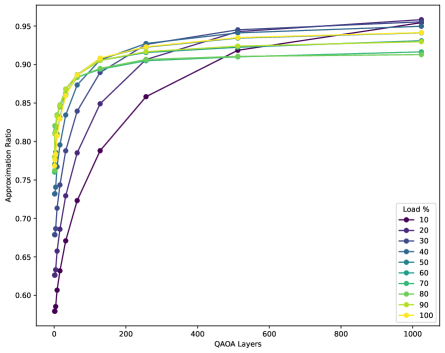
(a) QAOA Scaling performance for number of layers $p$.

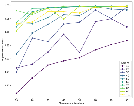
(b) SA Scaling performance for number of temperature iterations.

Figure 4: Model scaling performance showing the approximation ratio for 20 Qubits across all load percentages.

IV-D QAOA Parameters and Layers

To allow for a fair comparison between the classical approach and QAOA, we refrain from training the QAOA parameters beta and gamma, as this would distort the overall runtimes benefiting the QAOA. In line with the established ramp initialization motivated by a linear time evolution of the approximated adiabatic algorithm (cf. Ref. [23]) the parameters $\beta,\gamma\in\mathbb{R}^{p}$ for layer $k\in\left\{1,...,p\right\}$ are defined as $\gamma_{k}\coloneqq\frac{k}{p}$ (i.e., linearly rising in equally large steps from $0$ to $1$) and $\beta_{k}\coloneqq-\frac{p-k+1}{p}$ (i.e., linearly falling in equally large steps in terms of the absolute value from $-1$ to $0$). The negative sign for $\beta_{k}$ is a result of using the normal $R_{x}$ rotations for the mixer layer in the QAOA while making sure that the approximate adiabatic process starts in the groundstate (cf. Section II). A very positive aspect of avoiding runtime-heavy parameter training is the possibility of scaling up to a wide range of QAOA layers. To best explore performance scaling properties in a regime of deep QAOA layers, we investigate the number of layers in exponential steps ranging from $p=2^{0}=1$ to $p=2^{10}=1024$.

V Results

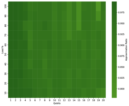
(a) QAOA Heatmap for $p=256$ layers.

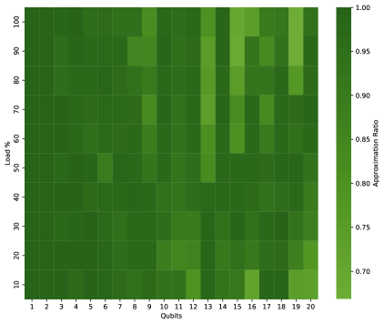
(b) SA Heatmap for $20$ temperature iterations.

Figure 5: Performance Heatmap showing the approximation ratio across all qubit and load percentage permutations. The colorbar is centered equally for both plots.

This section is structured in three parts, displaying results on the solution quality, the runtime complexity, a performance comparison on the different problem instances in terms of the approximation ratios, and finally the time to solution.

V-A Solution Quality

The solution quality for the SA approach largely depends on the number of temperature iterations. For the QAOA approach, the solution quality largely depends on the number of layers. In Figure 3b we explore the performance for various SA temperature iterations and in Figure 3a we explore the performance for various QAOA layers. To more accurately compare the two approaches we scale the number of temperature iterations exponentially by powers of 2, to match the scaling of the QAOA layers, and plot the four biggest models for both SA and QAOA. For SA we show 10, 20, 40, and 80 temperature iterations. For the QAOA we show 128, 256, 512, and 1024 layers. The results for every load configuration are averaged over all qubits, with the shaded regions showing the 95% confidence interval. SA has difficulty finding good solutions for the edge load configurations. It persists across all temperature iterations and is highlighted by the consistently concave shape of their curve. The QAOA results, on the other hand, have much less variation in results across all load configurations. This is reflected by the smaller spread in their results and the more constant performance across load configurations.

V-B Runtime Complexity

We now investigate the impact of the number of QAOA layers on performance more closely. Given the extreme speed of our algorithm and the lack of parameter training, we were able to increase the number of layers exponentially from $2^{0}=1$ to $2^{10}=1024$. The results for all these layers for 20 Qubits across all load configurations are shown in Figure 4a. The approximation ratio of the QAOA climbs continuously with increasing number of layers, achieving approximation ratios above 90% for every load configuration for both 512 and 1024 layers. While certain load configurations are more difficult at lower numbers of layers, the performance differential vanishes starting at 512 layers. With the two worst performing instances, 10% and 20% load, achieving among the highest results out of all configurations at 1024 layers.

The impact of the number of temperature iterations for SA, ranging from 10 to 80, for 20 Qubits across all load configurations is shown in Figure 4b. The results improved with an increasing number of iterations, but have a far wider spread, dependent on the specific load configuration. Even at 80 temperature iterations, the 10% and 20% load configurations underperform.

V-C Performance Comparison

The results for 256 QAOA layers and 20 SA temperature iterations are comparable as seen in the previous section on runtime complexity. They are both the third largest model in their respective approach given our exponential scaling making a comparison between them interesting in terms of performance and efficiency. While the previous plots analyzed the results for different load configurations averaged over all qubits, we will now analyze the detailed results across all 20 Qubits and 10 load configurations. The results for the 256 layer QAOA are plotted as a heatmap in Figure 5a. It shows that our QAOA-based approach performs significantly better than random, achieving approximation ratios around 90%. With many instances scoring even higher and approaching the ideal results. The worst performing instances still had approximation ratios around roughly 80%.

The results for the SA approach using 20 temperature iterations for all qubits and load configurations are shown in Figure 5b. SA is also able to achieve near-optimal results in some instances, however, it reaches values as low as 70% for its worst-performing instances. The spread in performance is noticeably bigger than for the QAOA. There is also a trend of underperformance in the load configurations near the top and bottom edges.

To highlight the difference in performance between the two approaches, in Figure 6 the SA results are subtracted from the QAOA results and plotted as a heatmap. The QAOA can outperform SA in some instances by as much as 15%, while SA is only able to beat the QAOA by roughly 5%. The heatmap also shows a pattern in performance differences, with the QAOA having better results clustered around the edges of the load configurations. This highlights the SA inconsistency with certain load configurations.

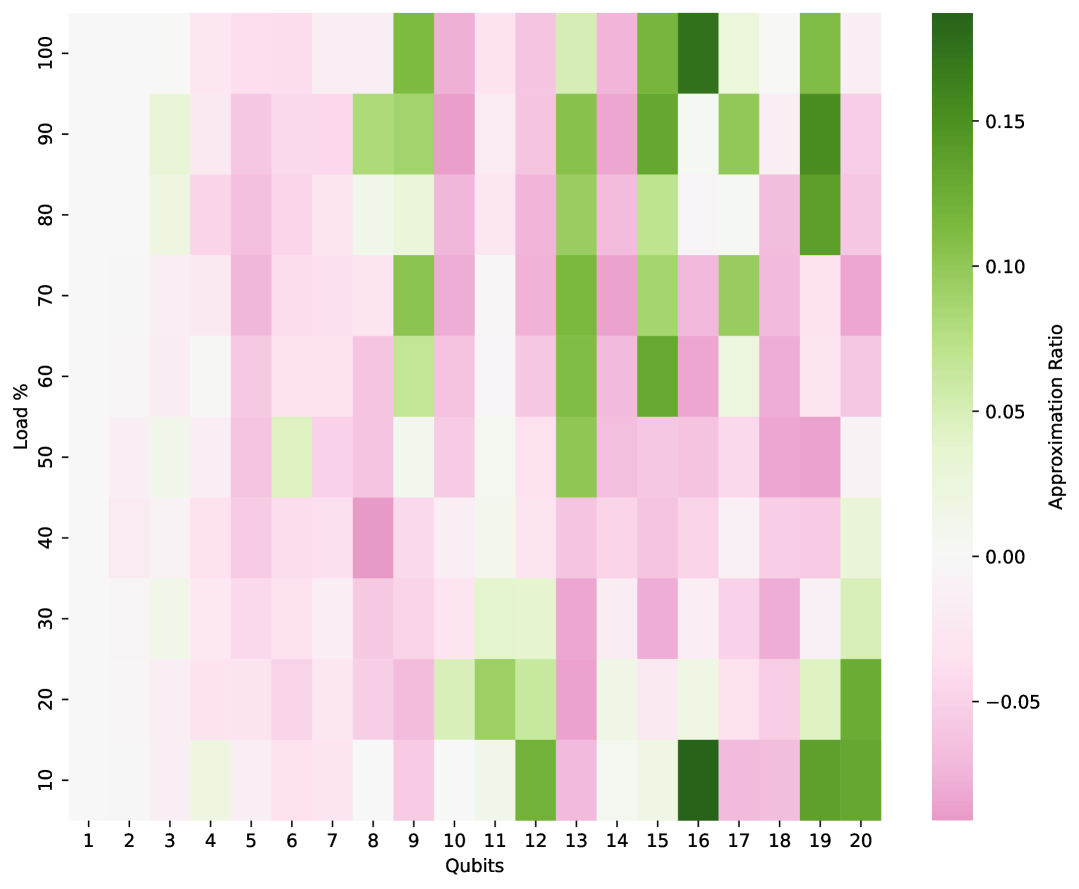
Figure 6: Performance difference heatmap between QAOA at $p=256$ layers and SA at $20$ temperature iterations. Positive values correspond to QAOA outperforming SA, negative values correspond to SA outperforming QAOA.

V-D Time to Solution

In Figure 7 we compare the efficiency of the two approaches, by plotting the time to solution. The threshold is set to 95% and the load configurations are averaged for every qubit. For every qubit, the minimum TTS is plotted for both SA and QAOA, with the data for all temperature iterations and QAOA layers being used in the analysis. The QAOA can consistently beat the SA at this threshold, except one outlier at 7 qubits which likely is irrelevant from a statistical perspective. The slopes of the fitted data show that the problem becomes more difficult with an increasing number of qubits, but not by a very large degree.

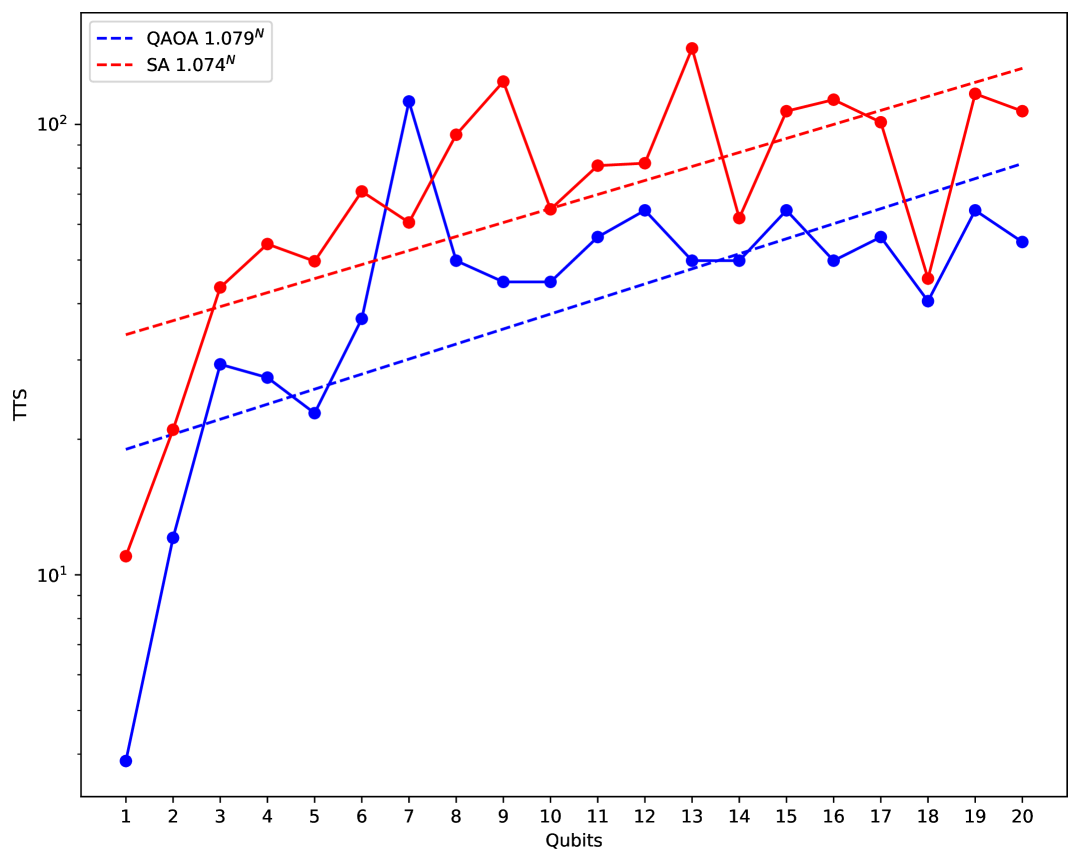
Figure 7: Time to solution for an approximation ratio threshold of $95\%$, averaging over all loads for each qubit. Both approaches show minimal exponential scaling and QAOA is slightly faster. The slope of the fitted line is displayed in the legend.

VI Discussion

The optimization component of the quantum simulation-based approach for the unit commitment is shown to be fast, efficient and very effective. The QAOA was able to scale to very high numbers of layers and consistently increase its performance with no parameter optimization whatsoever. Even difficult problem instances were solved to near optimal levels with enough layers. The lack of any optimization allows a practically arbitrary circuit depth, as we have shown by scaling the circuit depth exponentially. Compared to SA, the QAOA approach can offer comparable maximum results, while at the same time being far more stable across different problem instances.

In terms of efficiency, the QAOA was able to outperform the SA approach in time to solution for a 95% threshold. In numeric simulation, the QAOA has an intrinsic advantage in these statistical experiments as it can generate multiple thousands of samples from its measured state nearly instantaneously. The SA on the other hand requires a completely new run through the entire algorithm to generate additional samples, massively increasing its runtime and computational requirements. This enables the QAOA to generate a far more efficient and accurate probability estimates for sampling a state above a threshold. For the sake of a fair comparison however, both the QAOA and SA only used 10 samples for the TTS experiment.

When analyzing the performance in detail across every qubit and load permutation, the QAOA can achieve excellent results. In this granular view, it also demonstrates that it can achieve good solutions more reliably. While SA was able to find nearly optimal solutions for some permutations, it consistently struggled with certain problem instances (very small and very high load percentages). This was reflected clearly in its concave performance graph across different load configurations, even when averaged over all qubit values. In terms of wallclock runtime the 256 layer QAOA took about twice as long as one single 20 temperature iteration SA run. SA with 10 iterations to generate 10 samples thus ends up taking 5 times as long to run on the same machine. With an increasing number of samples, this difference will only become more pronounced.

With parameter optimization, which was entirely omitted, it is reasonable to assume that the QAOA would increase its performance even further (cf. Ref. [30, 31]). Thus not only becoming more effective but also more efficient in comparison to alternative approaches like SA, as it would be able to use a smaller number of layers to reach the previously unoptimized result quality.

VII Conclusion

The presented results show that the QAOA-based QuSO solver performs on par with the chosen classical baseline and in general, is able to solve all problem instances to a very high accuracy. Through the setup of the dataset, we incorporated practical relevance by real-world data. We can therefore conclude that the optimization component of the QuSO solver proposed in Ref [1] performs well, constituting a proof of concept. This underscores the potential of the proposed QuSO solver, such that not only provable speedups for the simulation component can be shown, but also near-optimal optimization performance.

The approach allowed us to scale to extremely large circuit depths, reaching 1024 QAOA layers. We were able to achieve excellent results without any parameter optimization by simply increasing the circuit depth and using a good heuristic parameter instantiation. Compared to SA our approach is competitive in result quality as shown in the achieved approximation ratio and efficiency as shown in the achieved time to solution for a 95% threshold. Furthermore, the QAOA delivered good results more consistently for all qubit and load permutations. SA consistently struggled to achieve a high approximation ratio with certain problem permutations, regardless of the number of temperature iterations.

Limitations of this work include the somewhat restricted scope and size of the problem instances. While additional datasets are available in literature, the limits on the size of the problem instance are harder to tackle, as the required classical precomputation of the complete solution space demands exponentially growing compute. Using HPC systems, the problem size could be scaled up to 40 or 50 qubits, but as our executions where limited to end-user hardware, only problems up to 20 qubits were practically feasible.

Appendix

The code can be accessed via this Github link: https://github.com/MaxiAdler/UCP-Paper

References

- [1] J. Stein, L. Müller et al., “Exponential quantum speedup for simulation-based optimization applications,” 2024.
- [2] A. W. Harrow, A. Hassidim et al., “Quantum algorithm for linear systems of equations,” Phys. Rev. Lett., vol. 103, p. 150502, Oct 2009.
- [3] A. Ambainis, “Variable time amplitude amplification and quantum algorithms for linear algebra problems,” in 29th International Symposium on Theoretical Aspects of Computer Science (STACS 2012), ser. Leibniz International Proceedings in Informatics (LIPIcs), C. Dürr and T. Wilke, Eds., vol. 14. Dagstuhl, Germany: Schloss Dagstuhl – Leibniz-Zentrum für Informatik, 2012, pp. 636–647.
- [4] D. W. Berry, A. M. Childs et al., “Hamiltonian simulation with nearly optimal dependence on all parameters,” in 2015 IEEE 56th Annual Symposium on Foundations of Computer Science, 2015, pp. 792–809.
- [5] A. M. Childs, R. Kothari et al., “Quantum algorithm for systems of linear equations with exponentially improved dependence on precision,” SIAM Journal on Computing, vol. 46, no. 6, pp. 1920–1950, 2017.
- [6] A. Gilyén, Y. Su et al., “Quantum singular value transformation and beyond: exponential improvements for quantum matrix arithmetics,” 2018.
- [7] Y. Subaşı, R. D. Somma et al., “Quantum algorithms for systems of linear equations inspired by adiabatic quantum computing,” Phys. Rev. Lett., vol. 122, p. 060504, Feb 2019.
- [8] L. Lin and Y. Tong, “Optimal polynomial based quantum eigenstate filtering with application to solving quantum linear systems,” Quantum, vol. 4, p. 361, Nov. 2020.
- [9] D. Orsucci and V. Dunjko, “On solving classes of positive-definite quantum linear systems with quadratically improved runtime in the condition number,” Quantum, vol. 5, p. 573, Nov. 2021.
- [10] A. Montanaro and L. Zhou, “Quantum speedups in solving near-symmetric optimization problems by low-depth qaoa,” 2024.
- [11] Y. Carson and A. Maria, “Simulation optimization: methods and applications,” in Proceedings of the 29th Conference on Winter Simulation, ser. WSC ’97. USA: IEEE Computer Society, 1997, p. 118–126.
- [12] R. H. Myers, D. C. Montgomery et al., Response surface methodology: process and product optimization using designed experiments. John Wiley & Sons, 2016.
- [13] V. O. Balabanov and R. T. Haftka, “Topology optimization of transport wing internal structure,” Journal of aircraft, vol. 33, no. 1, pp. 232–233, 1996.
- [14] M. R. Hestenes, E. Stiefel et al., “Methods of conjugate gradients for solving linear systems,” Journal of research of the National Bureau of Standards, vol. 49, no. 6, pp. 409–436, 1952.
- [15] https://icseg.iti.illinois.edu/ieee-57-bus-system/, accessed: 2024-11-14.
- [16] J. Stein, J. Blenninger et al., “Cuaoa: A novel cuda-accelerated simulation framework for the qaoa,” in 2024 IEEE International Conference on Quantum Computing and Engineering (QCE), vol. 2, 2024, pp. 280–285.
- [17] A. W. Harrow, A. Hassidim et al., “Quantum algorithm for linear systems of equations,” Phys. Rev. Lett., vol. 103, p. 150502, Oct 2009.
- [18] F. Gaitan, “Finding flows of a Navier–Stokes fluid through quantum computing,” npj Quantum Inf., vol. 6, no. 1, p. 61, 2020.
- [19] E. Farhi, J. Goldstone et al., “Quantum computation by adiabatic evolution,” 2000.
- [20] M. Born and V. Fock, “Beweis des Adiabatensatzes,” Zeitschrift für Phys., vol. 51, no. 3, pp. 165–180, 1928.
- [21] E. Farhi, J. Goldstone et al., “A quantum approximate optimization algorithm,” 2014.
- [22] A. Apte, S. H. Sureshbabu et al., “Iterative interpolation schedules for quantum approximate optimization algorithm,” 2025.
- [23] S. H. Sack and M. Serbyn, “Quantum annealing initialization of the quantum approximate optimization algorithm,” Quantum, vol. 5, p. 491, Jul. 2021.
- [24] S. Kirkpatrick, C. D. Gelatt et al., “Optimization by Simulated Annealing,” Science, vol. 220, no. 4598, pp. 671–680, May 1983, publisher: American Association for the Advancement of Science. doi: 10.1126/science.220.4598.671.
- [25] Y. Nourani and B. Andresen, “A comparison of simulated annealing cooling strategies,” Journal of Physics A: Mathematical and General, vol. 31, no. 41, pp. 8373–8385, Oct. 1998, doi: 10.1088/0305-4470/31/41/011.
- [26] “dwave-samplers,” Oct. 2023, https://github.com/dwavesystems/dwave-samplers.
- [27] R. D. Christie, “Power system test case archive,” 1993.
- [28] Y. Koç, M. Warnier et al., “A topological investigation of phase transitions of cascading failures in power grids,” Physica A: Statistical Mechanics and its Applications, vol. 415, pp. 273–284, 2014.
- [29] D. Bucher, N. Kraus et al., “Towards robust benchmarking of quantum optimization algorithms,” 2024.
- [30] V. Kremenetski, A. Apte et al., “Quantum alternating operator ansatz (qaoa) beyond low depth with gradually changing unitaries,” 2023.
- [31] V. Kremenetski, T. Hogg et al., “Quantum alternating operator ansatz (qaoa) phase diagrams and applications for quantum chemistry,” 2021.