Stochastic collocation schemes for Neural Field Equations with random data

Abstract

We develop and analyse numerical schemes for uncertainty quantification in neural field equations subject to random parametric data in the synaptic kernel, firing rate, external stimulus, and initial conditions. The schemes combine a generic projection method for spatial discretisation to a stochastic collocation scheme for the random variables. We study the problem in operator form, and derive estimates for the total error of the schemes, in terms of the spatial projector. We give conditions on the projected random data which guarantee analyticity of the semi-discrete solution as a Banach-valued function. We illustrate how to verify hypotheses starting from analytic random data and a choice of spatial projection. We provide evidence that the predicted convergence rates are found in various numerical experiments for linear and nonlinear neural field problems.

1 Introduction

Modelling brain dynamics and comprehending how uncertainties in the inputs affect quantities of interest (QOI) is a fundamental question in neuroscience. This field faces several challenges, including epistemic uncertainty arising from imperfect models, which are often phenomenological in nature. Additionally, the nonlocality of these models necessitates specialized numerical approaches.

In this paper we study uncertainty quantification (UQ) in a class of nonlinear brain activity models known as neural fields, which are integro-differential equations used as large-scale descriptions of neuronal activity. They model the cortex as a continuum, and provide a versatile tool to understand pattern formation on a variety of spatial domains [51, 2, 23, 14, 17].

Neural fields are amenable to functional and nonlinear analysis in simple cortices, and thus can be used to investigate fundamental mechanisms for the generation of brain activity. For instance, neural field simulations on spherical domains [44, 15, 49], or more realistic cortices [36, 41, 45] support several coherent structures observed experimentally, such as waves or stationary localised structures [33, 30, 32].

While a large body of work shows that nonlinearity and nonlocality are building blocks for patterns of neural activity, their robustness to noisy input data is still mostly unexplored. In the mathematical and computational neuroscience communities, Monte Carlo sampling is a popular approach to estimate mean and variance of QOI. Methods offering faster convergence rates, such as Stochastic Finite Elements or Stochastic Collocation, have been developed for applications in other branches of physical and life sciences (see [46, 34, 1] for textbooks discussing these methods). The literature on these schemes, however, focuses predominantly on Partial Differential Equations (PDEs) [52, 27, 13, 12, 26, 53, 31, 40, 39, 38, 29], and is not immediately applicable to neural field equations, even though UQ techniques for ODEs have recently been applied to connectomic ODE models of reaction–diffusion processes for neurodegenration [18].

A classical neural field problem is written in terms of an activity variable $u(x,t)$, modelling voltage or firing rate at time $t$ and position $x$ of a cortical domain $D\subset\mathbb{R}^{3}$. We consider (for now informally) a neural field subject to the following independent random data: an initial condition $v(x,\omega_{v})$, an external forcing $g(x,t,\omega_{g})$, a synaptic kernel $w(x,x^{\prime},\omega_{w})$, modelling connections from point $x^{\prime}$ to $x$ in $D$, and a firing rate function $f(u,\omega_{f})$, modelling how neurons transform input currents into spiking rates. We distinguish between a random linear neural field (RLNF, henceforth indicated with the index $\mathbb{L}=1$) in which the firing rate is deterministic and linear $f(u,\omega_{f})\equiv u$, and a random nonlinear neural field (RNNF, $\mathbb{L}=0$). Neural field problems with random input data read as follows: for fixed $v$, $w$, $g$, and $f$, we seek for a mapping $u\colon D\times J\times\Omega\to\mathbb{R}$ such that for $\operatorname{\mathbb{P}}$-almost all $\omega\in\Omega$ it holds

(1) $$\partial_{t}u(x,t,\omega)=-u(x,t,\omega)+g(x,t,\omega_{g})+\int_{D}w(x,x^{\prime},\omega_{w})f(u(x^{\prime},t,\omega),\omega_{f})\,dx^{\prime},$$

$$u(x,0,\omega)=v(x,\omega_{v}).$$

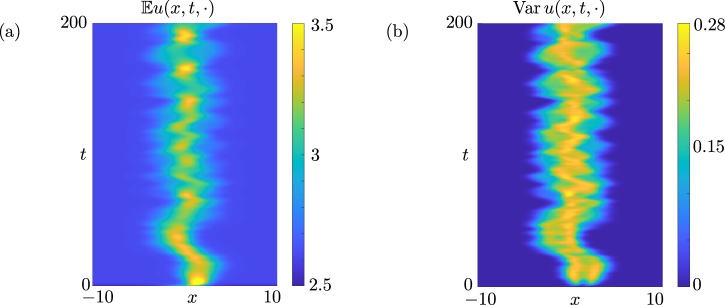
Figure 1: Expectation and variance of a solution $u$ to the nonlinear neural field Eq. 1 with random forcing. The problem is posed on a 1-dimensional ring $D=\mathbb{R}/L\mathbb{Z}$ of width $L=22$, and time interval $J=[0,200]$. Deterministic data is specified through an excitatory-inhibitory kernel $w(x,y)=W(x-y)$ with $W(z)=(2-z^{2})\exp(-z^{2})$, a sigmoidal firing rate $f(u)=[1+\exp(-20(u-10))]^{-1}$, and initial condition $v(x)=2.5+0.5/\cosh^{2}(0.5x)$. The external input is an oscillating pulse with random instantaneous speed $c$ depending on $6$ random variables: the forcing is given by $g(x,t,Y(\omega_{g}))$, where $g(x,t,y)=1.4\exp(-(x-c(t,y))^{2})$, $y=(c_{1},c_{2},c_{3},f_{1},f_{2},f_{3})$, $c(t,y)=\sum_{k=1}^{3}c_{k}\sin(2\pi t/f_{k})$. The random variables $Y_{i}$ are independently distributed with $Y_{i}\sim\mathcal{U}[\alpha_{i},\beta_{i}]$. The model is discretised in space using a spectrally convergent Fourier collocation scheme with $n=100$ gridpoints. Expectation and variance are computed with a stochastic collocation scheme, with a dense, tensor-product grid of 10 Gauss-Legendre points in each of the intervals $[\alpha_{i},\beta_{i}]$, for a total $10^{6}$ points. Parameters $[\alpha_{1},\beta_{1}]=[0,4]$, $[\alpha_{2},\beta_{2}]=[1/6,2/3]$, $[\alpha_{3},\beta_{3}]=[1/10,4/5]$, $[\alpha_{4},\beta_{4}]=[40,60]$, $[\alpha_{5},\beta_{5}]=[10,50/3]$, $[\alpha_{6},\beta_{6}]=[100,200]$.

We defer to later sections the probabilistic setting for data and solutions to the problem, and we view Eq. 1 as a prototype for studying forward UQ for spatio-temporal brain activity, as it encapsulates inputs and mathematical structure present in more realistic and involved neurobiological models. Recently, two stepping stones for investigating UQ problems in the form Eq. 1 have been laid. Firstly, spatial discretisations of deterministic problems have been investigated in abstract form [6]: following up from work by Atkinson [5], it is possible to derive convergence estimates for Collocation and Galerkin schemes, of Finite-Elements or Spectral type, as generic projection methods. Secondly, in [9] we studied Eq. 1 as a Cauchy problem with random data, posed on Banach spaces; in particular, we have established conditions on the input data that guarantee the $L^{p}$-regularity of the mapping $\omega\mapsto u({\mkern 2.0mu\cdot\mkern 2.0mu},{\mkern 2.0mu\cdot\mkern 2.0mu},\omega)$ in the natural function spaces for neural fields and for their spatially-discretised versions; further, the theory in [9] covers the case of finite-dimensional noise, which deals with inputs parametrised by a finite, possibly large, number of random variables.

We are thus in the position of analysing schemes that approximate statistics of QOI, which is the main goal of the present article. An example of these types of computations is given in Figure 1, where the mean and variance of $\omega\mapsto u(x,t,\omega)$ is approximated for a neural field equation posed on a simple 1D cortex (a ring), subject to a random forcing. The deterministic data used for the simulation (synaptic kernel, firing rate, and initial value) are frequently used in the mathematical neuroscience literature, and are such that the neural field supports a bump of localised activity (a steady state). The computation shows how this stationary pattern is affected by a random, pulsatile, sloshing external forcing. This setup is relevant to cortical processes associated to working memory associated to the brain navigational system, or oculomotor responses (we refer to [10] and references therein for further modelling and experimental work).

In Fig. 1 the system is discretised in space using a Chebyshev interpolatory projector from [6], and QOI are estimated with a Stochastic Collocation scheme in the spirit of the classical work by Babuška, Nobile, and Tempone [12]. This method is part of a family of schemes analysed here, that we call spatial-projection, stochastic-collocation schemes, in which stochastic collocation is paired to an arbitrary projection scheme, thus retaining the flexibility and generality of the framework in [6, 9].

The analysis of generic spatial-projection stochastic collocation schemes for neural fields is the main contribution of this paper. In the PDE literature cited above, the spatial projector is often an orthogonal projector, leading prevalently to Galerkin Finite Elements schemes. This approach, which has also been extended to time-dependent, linear parabolic PDEs by Zhang and Gunzburger [55], stems naturally from the deterministic functional setup, where schemes on nontrivial geometries are presented using weak formulations. Adapting this approach to neural fields comes with different challenges, and naturally brings a generalisation: it is possible to study in parallel neural fields as dynamical systems on the Banach phase spaces $\mathbb{X}=C(D)$ and $\mathbb{X}=L^{2}(D)$ [43, 25]; this dichotomy shows up also in their numerical treatment, which features a single projector $P_{n}$ on an $n$-dimensional subspace of $\mathbb{X}\in\{C(D),L^{2}(D)\}$, encompassing at once schemes in strong and weak form for collocation and Galerkin methods, respectively. The convergence rates of such schemes is determined in a unified manner, studying how $P_{n}$ approximates an element $v$ of the phase space, via an estimate of $\|P_{n}v-v\|$ [6].

Taking the literature on elliptic and parabolic PDEs as a guiding example [12, 55], we estimate the error $\|u-u_{n,q}\|$, measured in an appropriate norm, between the solution $u$ and an approximation $u_{n,q}$ which combines an $s(n)$-dimensional (interpolatory or orthogonal) spatial projection with a $d(q)$-dimensional interpolatory projection for the random variables, for some $s(n)$ and $d(q)$ with $s(n)\to\infty$ as $n\to\infty$ and $d(q)\to\infty$ as $q\to\infty$, respectively. We derive an error bound in terms of a spatial component $\|u-u_{n}\|$ and a stochastic collocation component $\|u_{n}-u_{n,q}\|$ with constants that are homogeneous in $q$ and $n$, respectively.

However, since the neural field theory is built around a generic projected dynamical system with random data, this leads to some differences from the PDE literature. For instance, no assumption can be made on the convergence of $\|P_{n}\|$ as $n\to\infty$, in contrast to existing literature using orthogonal projectors for which $\|P_{n}\|$ is bounded homogeneously in $n$. Keeping generality is valuable for neuroscience applications, because efficient schemes for neural fields use projectors that are not orthogonal, or for which the sequence $\{\|P_{n}\|\}_{n}$ is unbounded (the one used in Fig. 1 being one of them).

Existing literature on elliptic and parabolic PDEs derives exponential convergence rates in $q$ for $\|u_{n}-u_{n,q}\|$ by proving that analyticity of the random input data implies analyticity of $u$ [12, 55]. Our theory recovers analogous results for neural fields when $\{\|P_{n}\|\}_{n}$ is bounded in $n$, but is applicable to cases in which $\{\|P_{n}\|\}_{n}$ is unbounded, provided the random input data has sufficient spatial regularity. In particular, we give conditions on the projected random input data (for instance $P_{n}g$ and $P_{n}v$) which guarantee the analyticity of the spatially discretised solution $u_{n}$ as a function of the random variables. Because the derived estimates on the derivatives are homogeneous in $n$, the same occurs for the stochastic collocation error $\|u_{n}-u_{n,q}\|$, as required.

In addition, the treatment presented here does not assume Hilbert structure of the phase space $\mathbb{X}$ of the dynamical system with random data, leading to strong norms when $\mathbb{X}=C(D)$, a case that is frequent in neural field applications. To this end we use definitions and tools for Banach-space valued functions [16].

We derive error bounds for linear neural fields, without assuming dissipative dynamics, that is, without assuming that the underlying semigroup operator is contractive, in a sense that we make precise later. We link the lack of contractivity to time-dependent analyticity radii that shrink as time increases. We argue that, while analyticity results are in place for the nonlinear case, the sharp gradients induced by non-contractive dynamics is to be expected for nonlinear problems near bifurcation points. Finally, we provide evidence of exponential convergence rates in linear and nonlinear problems, and signpost a slower convergence rates near a bifurcating solution. Throughout the paper, we provide illustrative examples on how to check hypotheses on random data with affine and non-affine dependence on parameters, with various spatial projectors.

The paper is organised as follows: we set our notation in Section 2, and summarise hypotheses and results for neural fields with random data in Section 3. Our numerical scheme is introduced in Section 4, and analysed for linear problems in Section 5. Section 6 contains comments on the nonlinear problem, while Section 7 presents numerical experiments. We conclude in Section 8.

2 Notation

We set $\mathbb{N}_{n}=\{1,\ldots,n\}$ and $\mathbb{N}_{>n}=\mathbb{N}\setminus\mathbb{N}_{n}$ (we similarly use $\mathbb{N}_{\geq n}$, and $\mathbb{Z}_{\geq 0}$, where $\mathbb{Z}$ denotes the integers). The symbol $\mathbb{X}$ denotes a Banach space of functions defined on some $D\subset\mathbb{R}^{\textrm{dim}}$, while $J=[0,T]\subset\mathbb{R}$ is used for time intervals. We denote by $C^{k}(\Gamma,\mathbb{B})$ the space of $k$-times continuously differentiable functions on a subspace $\Gamma\subseteq\mathbb{R}^{m}$ to a Banach space $\mathbb{B}$, with norm $\|v\|_{C^{k}(\Gamma,\mathbb{B})}=\max_{j\in\mathbb{N}_{k}}\sup_{y\in\Gamma}\|v^{(j)}(y)\|_{\mathbb{B}}$. We use the shortcuts $C(\Gamma,\mathbb{B}):=C^{0}(\Gamma,\mathbb{B})$ and $C^{k}(\Gamma):=C^{k}(\Gamma,\mathbb{R})$.

The set of bounded linear operators on $\Gamma$ to $\mathbb{B}$, with standard operator norm, is denoted by $BL(\Gamma,\mathbb{B})$. When it is important to emphasise that derivatives are understood in the sense of Fréchet, we indicate the $j$th Frechét derivative of $v\colon\Gamma\to\mathbb{B}$ at $y$ by $d^{\,j}v[y]\colon\Gamma\to BL(\Gamma^{k},\mathbb{B})$.

We use the symbol $u$ for different, interrelated mappings, the most basic being $u(x,t,\omega)$ for the neural field solution as a mapping from $D\times J\times\Omega$ to $\mathbb{R}$. We also progressively “slice” this function from the leftmost argument, and so $u(t,\omega)$ is a mapping on $J\times\Omega$ to $\mathbb{X}$, so that, with a little abuse of notation, $u(t,\omega)(x)=u(x,t,\omega)$; further, we may use $u(\omega)$ for the corresponding mapping on $\Omega$ to $\mathbb{B}$, where $\mathbb{B}$ is a suitable Banach space of functions on $D\times J$, for instance $\mathbb{B}=C(J,\mathbb{X})$, and so $u(\omega)(x,t)=u(x,t,\omega)$. In addition, it is necessary to consider finite-dimensional noise random fields, so that $u(x,t,\omega)=\tilde{u}(x,t,Y(\omega))$ for suitable choices of the function $\tilde{u}$ and the $\mathbb{R}^{m}$-valued random variables $Y$. We often omit the tilde, but we warn the reader when necessary, to help disambiguating the overloaded symbol $u$.

For a Banach space $\mathbb{B}$, and a weight function $\sigma\colon\Gamma\to\mathbb{R}_{\geq 0}$ we make use of the weighted function spaces,

(2) $$C^{0}_{\sigma}(\Gamma,\mathbb{B})=\Big{\{}v:\Gamma\rightarrow\mathbb{B},\quad v\in C^{0}(\Gamma,\mathbb{B}),\quad\|u\|_{C^{0}(\Gamma,\mathbb{B})}:=\max_{y\in\Gamma}\|\sigma(y)v(y)\|_{\mathbb{B}}<\infty\Big{\}},$$

and

(3) $$C^{k}_{\sigma}(\Gamma,\mathbb{B})=\Big{\{}v:\Gamma\rightarrow\mathbb{B}, v k$$ is times differentiable,

$$\max_{y\in\Gamma}\bigl{\|}\,\sigma(y)\,d^{\,j}v[y]\,\bigr{\|}_{BL(\Gamma^{k},\mathbb{B})}<\infty\quad\text{for all}\quad j\in\mathbb{N}_{k}\Big{\}},$$

with norm $\|v\|_{C^{k}_{\sigma}(\Gamma,\mathbb{B})}=\max_{j\in\mathbb{N}_{k}}\max_{y\in\Gamma}\|\sigma(y)d^{\,j}v[y]\|_{BL(\Gamma^{k},\mathbb{B})}$.

We denote Bochner spaces of $\mathbb{B}$-valued random variables on a probability space $(\Omega,\mathcal{F},\operatorname{\mathbb{P}})$ as $L^{p}(\Omega,\mathcal{F},\operatorname{\mathbb{P}};\mathbb{B})$, or simply $L^{p}(\Omega,\mathbb{B})$, where $p\in[0,\infty]$; these spaces are the equivalence classes of strongly $\mathbb{B}$-valued random variables endowed with norms

$$\|u\|_{L^{p}(\Omega,\mathbb{B})}=(\operatorname{\mathbb{E}}\|u\|^{p})^{1/p}=\bigg{(}\int_{\Omega}\|u(\omega)\|^{p}_{\mathbb{B}}\,d\operatorname{\mathbb{P}}(\omega)\bigg{)}^{1/p}\qquad p\in[0,\infty),$$

$$\|u\|_{L^{\infty}(\Omega,\mathbb{B})}=\operatorname*{\mathbb{P}-ess\,sup}_{\omega\in\Omega}\|u(\omega)\|_{\mathbb{B}}.$$

For a given probability density $\rho\colon\Gamma\subseteq\mathbb{R}^{m}\to\mathbb{R}_{\geq 0}$ we set $L^{p}_{\rho}(\Gamma,\mathbb{B}):=L^{p}(\Gamma,\mathcal{B}(\mathbb{R}^{m}),\rho dy,\mathbb{B})$.

3 Hypotheses and results for neural fields with random data

We review the functional setup and standing hypotheses for the study of neural fields with random data, as obtained in [9]. We begin by discussing the spatial and temporal domains of the neural field equation.

[Spatio-temporal domain] It holds $(x,t)\in D\times J$, where $D\subset\mathbb{R}^{\textrm{dim}}$ is a compact domain with piecewise smooth boundary, and $J=[0,T]\subset\mathbb{R}$.

We formalise random data in the neural field equations similarly to the linear parabolic PDE case [55], hence we consider the probability spaces $(\Omega_{w},\mathcal{F}_{w},\operatorname{\mathbb{P}}_{w})$, $(\Omega_{f},\mathcal{F}_{f},\operatorname{\mathbb{P}}_{f})$, $(\Omega_{g},\mathcal{F}_{g},\operatorname{\mathbb{P}}_{g})$, and $(\Omega_{v},\mathcal{F}_{v},\operatorname{\mathbb{P}}_{v})$ or, compactly $\{(\Omega_{\alpha},\mathcal{F}_{\alpha},\operatorname{\mathbb{P}}_{\alpha})\colon\alpha\in\mathbb{U}\}$, with $\mathbb{U}\subseteq\{w,f,g,v\}.$ We introduce

(4) $$w\colon D\times D\times\Omega_{w}\to\mathbb{R}, f\colon\mathbb{R}\times\Omega_{f}\to\mathbb{R},$$

$$g\colon D\times J\times\Omega_{g}\to\mathbb{R}, v\colon D\times\Omega_{v}\to\mathbb{R},$$

and we are interested in how uncertainty in the data is propagated by the neural field model Eq. 1. We recall that the index $\mathbb{L}=1$ indicates linear and deterministic firing rates, $f(u)=u$, and $\mathbb{L}=0$ is used for realisations $u\mapsto f(u,\omega_{f})$ of the firing rate are nonlinear.

We assume that sources of noise are independent, as follows. [Independence] The random fields $w$, $f$, $g$, $v$ are mutually independent: the event space $\Omega$, $\sigma$-algebra $\mathcal{F}$, and probability measure $\operatorname{\mathbb{P}}$ are given by

$$\Omega=\mathop{\vphantom{\sum}\mathchoice{\vbox{\hbox{\begin{picture}(1.0,1.0)\roundcap \Line(.1,.1)(.9,.9) \Line(.1,.9)(.9,.1) \end{picture}}}}{\vbox{\hbox{\begin{picture}(1.0,1.0)\roundcap \Line(.1,.1)(.9,.9) \Line(.1,.9)(.9,.1) \end{picture}}}}{\vbox{\hbox{\begin{picture}(1.0,1.0)\roundcap \Line(.1,.1)(.9,.9) \Line(.1,.9)(.9,.1) \end{picture}}}}{\vbox{\hbox{\begin{picture}(1.0,1.0)\roundcap \Line(.1,.1)(.9,.9) \Line(.1,.9)(.9,.1) \end{picture}}}}}\slimits@_{\alpha\in\mathbb{U}}\Omega_{\alpha},\qquad\mathcal{F}=\mathop{\vphantom{\sum}\mathchoice{\vbox{\hbox{\begin{picture}(1.0,1.0)\roundcap \Line(.1,.1)(.9,.9) \Line(.1,.9)(.9,.1) \end{picture}}}}{\vbox{\hbox{\begin{picture}(1.0,1.0)\roundcap \Line(.1,.1)(.9,.9) \Line(.1,.9)(.9,.1) \end{picture}}}}{\vbox{\hbox{\begin{picture}(1.0,1.0)\roundcap \Line(.1,.1)(.9,.9) \Line(.1,.9)(.9,.1) \end{picture}}}}{\vbox{\hbox{\begin{picture}(1.0,1.0)\roundcap \Line(.1,.1)(.9,.9) \Line(.1,.9)(.9,.1) \end{picture}}}}}\slimits@_{\alpha\in\mathbb{U}}\mathcal{F}_{\alpha},\qquad\operatorname{\mathbb{P}}=\prod_{\alpha\in\mathbb{U}}\operatorname{\mathbb{P}}_{\alpha},\qquad\quad\mathbb{U}=\begin{cases}\{w,g,v\}&\text{if $\mathbb{L}=1$,}\\[5.0pt] \{w,f,g,v\}&\text{if $\mathbb{L}=0$.}\end{cases}$$

The theory in [6] casts the neural field problem in operator form as an ODE on a Banach space $\mathbb{X}$ with random data. Following this approach, we deal concurrently with two common functional setups of this problem, as is seen in the next hypothesis.

[Phase space] The phase space is either $\mathbb{X}$ = $C(D)$, the space of continuous functions on $D$ endowed with the supremum norm $\|{\mkern 2.0mu\cdot\mkern 2.0mu}\|_{\infty}$, or $\mathbb{X}=L^{2}(D)$, the Lebesgue space of square-integrable functions on $D$, endowed with the standard Lebesgue norm $\|{\mkern 2.0mu\cdot\mkern 2.0mu}\|_{2}$. We will compactly write $\mathbb{X}\in\{C(D),L^{2}(D)\}$.

With reference to Eq. 1, the Banach space $\mathbb{X}$ sets the function space for realisations of $v({\mkern 2.0mu\cdot\mkern 2.0mu},\omega_{v})$, the initial condition, $g({\mkern 2.0mu\cdot\mkern 2.0mu},t,\omega_{g})$, the forcing at time $t$, and $u({\mkern 2.0mu\cdot\mkern 2.0mu},t,\omega)$, the solution at time $t$. Realisations of the synaptic kernel $w({\mkern 2.0mu\cdot\mkern 2.0mu},{\mkern 2.0mu\cdot\mkern 2.0mu},\omega_{w})$ are bivariate functions, and therefore require a separate function space dependent on the choice of $\mathbb{X}$, denoted by $\mathbb{W}(\mathbb{X})$, or simply $\mathbb{W}$, and defined as

$$\mathbb{W}(\mathbb{X}):=\begin{cases}\displaystyle{\Big{\{}k\in C(D,L^{1}(D))\colon\lim_{h\to 0}\nu(h;k)=0\Big{\}},}&\text{if $\mathbb{X}=C(D)$,}\\[10.00002pt] L^{2}(D\times D)&\text{if $\mathbb{X}=L^{2}(D)$,}\\ \end{cases}$$

in which

$$\nu(h;k)=\max_{x,z\in D}\max_{\|x-z\|_{2}\leq h}\int_{D}|k(x,x^{\prime})-k(z,x^{\prime})|\,dx^{\prime},\qquad h\in\mathbb{R}_{\geq 0},$$

with norm

$$\|k\|_{\mathbb{W}}=\begin{cases}\|k\|_{C(D,L^{1}(D))}&\text{if $\mathbb{X}=C(D)$,}\\ \|k\|_{L^{2}(D\times D)}&\text{if $\mathbb{X}=L^{2}(D)$.}\\ \end{cases}$$

With these preparations Eq. 1 is written in operator form, as as a Cauchy problem on $\mathbb{X}$ with random data, as follows:

(5) $$u^{\prime}(t,\omega)=N(t,u(t,\omega),\omega_{w},\omega_{f},\omega_{g}),\qquad t\in J,$$

$$u(0,\omega)=v(\omega_{v}),$$

in which the operator $N$ is defined as

$$N\colon J\times\mathbb{X}\times\Omega_{w}\times\Omega_{f}\times\Omega_{g}\to\mathbb{X}\qquad N(t,u,\omega_{w},\omega_{f},\omega_{g})=-u+W(\omega_{w})F(u,\omega_{f})+g(t,\omega_{g}),$$

and realisations $W(\omega_{w})$ are bounded linear operators associated to the kernel realisations $w({\mkern 2.0mu\cdot\mkern 2.0mu},{\mkern 2.0mu\cdot\mkern 2.0mu},\omega_{w})$. Specifically one sets $W(\omega_{w})=H(w({\mkern 2.0mu\cdot\mkern 2.0mu},{\mkern 2.0mu\cdot\mkern 2.0mu},\omega_{w}))$, where

(6) $$H\colon\mathbb{W}\to K(\mathbb{X})\subset BL(\mathbb{X}),\qquad H(k)(v)=\int_{D}k({\mkern 2.0mu\cdot\mkern 2.0mu},x^{\prime})v(x^{\prime})\,dx^{\prime},$$

in which $K(\mathbb{X})$ is the space of compact operators on $\mathbb{X}$ to itself, hence

(7) $$W\colon\Omega_{w}\to K(\mathbb{X})\subset BL(\mathbb{X}),\qquad W(\omega_{w})v=\int_{D}w({\mkern 2.0mu\cdot\mkern 2.0mu},x^{\prime},\omega_{w})v(x^{\prime})\,dx^{\prime}.$$

Further the realisations $F({\mkern 2.0mu\cdot\mkern 2.0mu},\omega_{f})$ come from the firing rate realisations $f({\mkern 2.0mu\cdot\mkern 2.0mu},\omega_{f})$, as follows

(8) $$F\colon\mathbb{X}\times\Omega_{f}\to\mathbb{X},\qquad F(u,\omega_{f})(x):=\begin{cases}u(x)&\text{if $\mathbb{L}=1$,}\\ f(u(x),\omega_{f})&\text{if $\mathbb{L}=0$.}\end{cases}$$

In passing, we note that we often write $N({\mkern 2.0mu\cdot\mkern 2.0mu},{\mkern 2.0mu\cdot\mkern 2.0mu},\omega)$, instead of $N({\mkern 2.0mu\cdot\mkern 2.0mu},{\mkern 2.0mu\cdot\mkern 2.0mu},\omega_{w},\omega_{f},\omega_{g})$, for simplicity.

We work with $L^{p}$-regular input data, as indicated by the next hypothesis. [$L^{p}$-regularity of random data] It holds that either

$$\mathbb{L}=1,\quad w\in L^{\infty}(\Omega_{w},\mathbb{W}),\quad g\in L^{p}(\Omega_{g},C^{0}(J,\mathbb{X})),\quad v\in L^{p}(\Omega_{v},\mathbb{X}),$$

or

$$\mathbb{L}=0,\quad w\in L^{p}(\Omega_{w},\mathbb{W}),\quad f\in L^{p}(\Omega_{f},BC^{1}(\mathbb{R})),\quad g\in L^{p}(\Omega_{g},C^{0}(J,\mathbb{X})),\quad v\in L^{p}(\Omega_{v},\mathbb{X}),$$

Because Section 3 implies [9, Hypothesis 3.5], we can use directly [9, Theorems 4.2 and 4.5] on the well-posedness of Eq. 5, and the measurability and regularity of its solutions.

Theorem 3.1 (Abridginng [9, Theorems 4.2 and 4.5] on solutions to neural fields with random data).

Under Sections 3 to 3 there exists a -almost unique $u\in L^{p}(\Omega,C^{1}(J,\mathbb{X}))$ satisfying Eq. 5 -almost surely, that is, satisfying , with

$$B_{0}=\{\omega\in\Omega\colon u(0,\omega)=v(\omega_{v})\},\qquad B_{J}=\{\omega\in\Omega\colon u^{\prime}({\mkern 2.0mu\cdot\mkern 2.0mu},\omega)=N({\mkern 2.0mu\cdot\mkern 2.0mu},u({\mkern 2.0mu\cdot\mkern 2.0mu},\omega),\omega_{w},\omega_{f},\omega_{g})\text{ on $J$}\}.$$

As in the related PDE literature [52, 13, 12, 53, 46, 34, 1], we are interested in exploring problems with finite-dimensional random data. Therefore, we assume that, for instance, the initial condition $v(x,\omega_{v})$ depends on $m_{v}$ random parameters, which we denote $Y_{v}$, and similar for other sources of randomness in the model. We define finite-dimensional noise as in [34, Definition 9.38], and we state our hypothesis for finite-dimensional noise in neural fields.

Definition 3.2 ($m$-dimensional, $p$th-order, $\mathbb{B}$-valued noise).

Let $m,k\in\mathbb{N}$, and $\mathbb{B}$ be a Banach space. Further, let $\{Y_{k}\}$, $k\in\mathbb{N}_{m}$ be a collection of $m$ random variables $Y_{k}\colon\Omega\to\Gamma_{k}\subset\mathbb{R}$. A random variable $f\in L^{p}(\Omega,\mathbb{B})$ of the form $f({\mkern 2.0mu\cdot\mkern 2.0mu},Y(\omega))$, where $Y=(Y_{1},\ldots,Y_{m})\colon\Omega\to\Gamma=\Gamma_{1}\times\dots\times\Gamma_{m}$, is called an $m$-dimensional, $p$th-order, $\mathbb{B}$-valued noise. We abbreviate this by saying that $f\in L^{p}(\Omega,\mathbb{B})$ is $m$-dimensional noise.

[Finite-dimensional noise random data] The random data in Section 3 is finite-dimensional noise of the form

$$w({\mkern 2.0mu\cdot\mkern 2.0mu},{\mkern 2.0mu\cdot\mkern 2.0mu},\omega_{w})=\tilde{w}({\mkern 2.0mu\cdot\mkern 2.0mu},{\mkern 2.0mu\cdot\mkern 2.0mu},Y_{w}(\omega_{w})), Y_{w}\colon\Omega_{w}\to\Gamma_{w}\subset\mathbb{R}^{m_{w}}, Y_{w}\sim\rho_{w},$$

$$f({\mkern 2.0mu\cdot\mkern 2.0mu},\omega_{f})=\tilde{f}({\mkern 2.0mu\cdot\mkern 2.0mu},Y_{f}(\omega_{f})), Y_{f}\colon\Omega_{f}\to\Gamma_{f}\subset\mathbb{R}^{m_{f}}, Y_{f}\sim\rho_{f},$$

$$g({\mkern 2.0mu\cdot\mkern 2.0mu},{\mkern 2.0mu\cdot\mkern 2.0mu},\omega_{g})=\tilde{g}({\mkern 2.0mu\cdot\mkern 2.0mu},{\mkern 2.0mu\cdot\mkern 2.0mu},Y_{g}(\omega_{g})), Y_{g}\colon\Omega_{g}\to\Gamma_{g}\subset\mathbb{R}^{m_{g}}, Y_{g}\sim\rho_{g},$$

$$v({\mkern 2.0mu\cdot\mkern 2.0mu},\omega_{v})=\tilde{v}({\mkern 2.0mu\cdot\mkern 2.0mu},Y_{v}(\omega_{v})), Y_{v}\colon\Omega_{v}\to\Gamma_{v}\subset\mathbb{R}^{m_{v}}, Y_{v}\sim\rho_{v}.$$

The finite-dimensional noise assumption may hold for affine- or non-affine parameter dependence [12]. We present two examples for neural fields, which are later used for checking hypotheses in Section 5.2.1 and presenting numerical experiments in Section 7.

Example 3.3 (Affine parameter dependence).

Consider initial conditions in the form of a Karhunen-Loeve expansion of the form

(9) $$v(x,\omega_{v})=b_{0}(x)+\sum_{j\in\mathbb{N}_{m_{v}}}b_{j}(x)Y_{j}(\omega_{v}),\quad Y_{j}\stackrel{{\scriptstyle i.i.d}}{{\sim}}\mathcal{N}(0,1),\quad j\in\mathbb{N}_{m_{v}},\quad x\in D=[-1,1],$$

which is $m_{v}$-dimensional noise with $(y_{1},\ldots,y_{m_{v}})\in\Gamma_{v}=\mathbb{R}^{m}$, and in which the spatial regularity is controlled by $\{b_{j}\}_{j\in\mathbb{Z}_{m}}\subset\mathbb{X}$. In this case the mapping $y\mapsto\tilde{v}({\mkern 2.0mu\cdot\mkern 2.0mu},y)$ is affine.

Example 3.4 (Non-affine parameter dependence).

Consider the random external input

(10) $$g(x,t,\omega_{g})=e^{tY(\omega_{g})}\bigl{[}(Y(\omega_{g})+1)\sin(4\pi x)+x/(2\pi)\bigr{]}\quad x\in D=[-1,1],\quad t\in J=[0,T],$$

with $Y\sim\mathcal{U}[\alpha,\beta]$ or $Y\sim\mathcal{N}(0,\sigma)$. This forcing is $1$-dimensional noise with $y\in\Gamma_{g}=[\alpha,\beta]\subset\mathbb{R}$ or $\Gamma_{g}=\mathbb{R}$, and is used in the numerical example in Section 7.1.

In addition to finite-dimensionality of the noise, Definition 3.2 prescribes that each random variable $Y_{\alpha}$ has density $\rho_{\alpha}$, $\alpha\in\mathbb{U}$. It is possible to reformulate the neural field problem under the finite-dimensional noise assumption: all random variables are collected in a vector,

$$Y\colon\Omega\to\Gamma=\Gamma_{1}\times\ldots\times\Gamma_{m}\subset\mathbb{R}^{m},\qquad m=\sum_{\alpha\in\mathbb{U}}m_{\alpha},\qquad Y\sim\rho=\prod_{\alpha\in\mathbb{U}}\rho_{\alpha},$$

and one can express the neural field problem, in operator form, in terms of a deterministic function $\hat{u}({\mkern 2.0mu\cdot\mkern 2.0mu},{\mkern 2.0mu\cdot\mkern 2.0mu},y)$, using deterministic inputs $\tilde{w}$, $\tilde{f}$, $\tilde{g}$, and $\tilde{v}$ in place of the original inputs. We refer to [9, Section 5] for the reformulation of the neural field problem with finite-dimensional noise, which we present below. We highlight that tildes or hats are henceforth omitted for notational simplicity, as the problem formulation below can be taken as the starting point for investigating the problem in parametric form.

Problem 3.5 (Neural field problem with finite-dimensional noise).

Fix $\mathbb{L}$, $w$, $g$, $v$, and if $\mathbb{L}=0$, f. Given a density $\rho$ for the random variable $Y$, find $u\colon J\times\Gamma\to\mathbb{X}$ such that

(11) $$\begin{aligned} &u^{\prime}(t,y)=N(t,u(t,y),y),&t\in J,\\ &u(0,y)=v(y),&\end{aligned}\qquad\textrm{$\rho\,dy$-a.e. in $\Gamma$.}\\$$

The result below from [9], addresses well-posedness and regularity of the parametrised problem. The result is given in terms of Banach space-valued functions on $(\Gamma,\mathcal{B}(\mathbb{R}^{m}),\rho dy)$, for instance $v\in L_{\rho}(\Gamma,\mathbb{X}):=L^{p}(\Gamma,\mathcal{B}(\mathbb{R}^{m}),\rho dy,\mathbb{X})$.

Corollary 3.6 (Abridged [9, Corollary 5.1] on $L^{p}_{\rho}$-regularity with finite-dimensional noise).

Under Sections 3 to 3.2, it holds $w\in L^{\infty}_{\rho}(\Gamma,\mathbb{W})$ (if $\mathbb{L}=1)$ or $w\in L^{p}_{\rho}(\Gamma,\mathbb{W})$ (if $\mathbb{L}=0)$, $f\in L^{p}_{\rho}(\Gamma,BC(\mathbb{R}))$, $g\in L^{p}_{\rho}(\Gamma,C^{0}(J,\mathbb{X}))$, and $v\in L^{p}_{\rho}(\Gamma,\mathbb{X})$. Further, Problem 3.5 has a unique solution $u\in L^{p}_{\rho}(\Gamma,C^{1}(J,\mathbb{X}))$.

4 Spatial-projection stochastic-collocation scheme

We aim to construct a numerical approximation to the solution $u$ to Eq. 11 with well-defined mean and variance and, using Corollary 3.6, we seek for an approximation in a subspace of $L^{2}_{\rho}(\Gamma,C^{1}(J,\mathbb{X}))$. We intend to treat the spatial coordinate $x$ and the stochastic coordinate $y$ differently, so it is natural to work in $C^{1}(J,\mathbb{X})\otimes L^{2}_{\rho}(\Gamma)$, which is isometrically isomorphic to the original space $L^{2}_{\rho}(\Gamma,C^{1}(J,\mathbb{X}))$ [20, Sections 7.1–7.2]. Since the two spaces can be identified, a typical element of $u\in C^{1}(J,\mathbb{X})\otimes L^{2}_{\rho}(\Gamma)$, of the form $u=\sum_{j}A_{j}\otimes\psi_{j}=\sum_{j}A_{j}\psi_{j}$, can be measured using the norm on $L^{2}_{\rho}(\Gamma,C^{1}(J,\mathbb{X}))$.

We look for an approximation $u_{n,q}$ in $C^{1}(J,\mathbb{X}_{n})\otimes\mathcal{P}_{q}(\Gamma)$, where $\mathbb{X}_{n}\subset\mathbb{X}$ and $\mathcal{P}_{q}(\Gamma)\subset L^{2}_{\rho}(\Gamma)$ are finite-dimensional subspaces, whose definition will be made precise later, of dimension $s(n)$ and $d(q)$, respectively. The scheme proceeds in two steps, which are now introduced in detail:

• Step 1: construct an approximation $u_{n}({\mkern 2.0mu\cdot\mkern 2.0mu},y)$ in $C^{1}(J,\mathbb{X}_{n})$ to $u$ in $C^{1}(J,\mathbb{X})$ by a collocation scheme with grid $\{x_{i}\colon i\in\mathbb{N}_{s(n)}\}\subset D$

  $$u^{\prime}_{n}(t,y)(x_{i})=N(t,u_{n}(t,y))(x_{i}),\qquad u_{n}(0,y)(x_{i})\qquad(t,i,y)\in J\times\mathbb{N}_{s(n)}\times\Gamma$$

  or by a Galerkin scheme using test functions $\{\varphi_{i}\colon i\in\mathbb{N}_{s(n)}\}\subset\mathbb{X}_{n}$,

  $$\bigl{\langle}\varphi_{i},u^{\prime}_{n}(t,y)-N(t,u_{n}(t,y))\bigr{\rangle}_{\mathbb{X}}=0,\qquad\langle\varphi_{i},u_{n}(0,y)\rangle_{\mathbb{X}}=0,\qquad(t,i,y)\in J\times\mathbb{N}_{s(n)}\times\Gamma.$$

• Step 2: Collocate one of the schemes in step 1 on the zeros of orthogonal polynomials $\{y_{k}:k\in\mathbb{N}_{d(q)}\}$ and build $u_{n,q}$ using the collocated solutions

  $$u_{n,q}(t,y)=\sum_{k\in\mathbb{N}_{d(q)}}u_{n}(t,y_{k})l_{k}(y),$$

  where $\{l_{k}\}\subset\mathcal{P}_{q}(\Gamma)$ are Lagrange polynomials with nodes $\{y_{k}\}$.

4.1 Step 1: spatial projection

Schemes for neural fields of collocation and Galerkin type can be expressed using projectors  [6]. We consider a family of subspaces $\{\mathbb{X}_{n}\colon n\in\mathbb{N}\}\subset\mathbb{X}$, $\mathbb{X}_{n}:=\operatorname{Span}\{\varphi_{j}\colon j\in\mathbb{N}_{s(n)}\}$ with $\dim\mathbb{X}_{n}=:s(n)\to\infty$ as $n\to\infty$ and such that $\overline{\cup_{n\in\mathbb{N}}\mathbb{X}_{n}}=\mathbb{X}$. On each $\mathbb{X}_{n}$ we place the norm $\|{\mkern 2.0mu\cdot\mkern 2.0mu}\|_{\mathbb{X}}$. A corresponding family of projectors $\{P_{n}\colon n\in\mathbb{N}\}$ satisfies, for any $n\in\mathbb{N}$, $P_{n}\in BL(\mathbb{X},\mathbb{X}_{n})$, $\|P_{n}\|\geq 1$, and $P_{n}v=v$ for all $v\in\mathbb{X}_{n}$ [5], with

$$P_{n}\colon\mathbb{X}\to\mathbb{X}_{n}\qquad(P_{n}v)(x)=\sum_{j\in\mathbb{N}_{s(n)}}V_{j}\varphi_{j}(x)\qquad(x,n)\in D\times\mathbb{N}.$$

Interpolatory projectors define collocation schemes: we set $\mathbb{X}=C(D)$, $\varphi_{j}=\ell_{j}$, the $j$th Lagrange polynomial with nodes $\{x_{j}\}\subset D$, leading to $V_{j}=v(x_{j})$. Orthogonal projectors define Galerkin schemes: we set $\mathbb{X}=L^{2}(D)$ and $V_{j}=\langle v,\varphi_{j}\rangle_{\mathbb{X}}$. For details and examples we refer to [4, 3, 6]. A collocation or Galerkin scheme for Eq. 11 is written in abstract form as [6]

(12) $$\begin{aligned} &u_{n}^{\prime}(t,y)=P_{n}N(t,u_{n}(t,y),y),&t\in J,\\ &u_{n}(0,y)=P_{n}v(y),\end{aligned}\qquad\textrm{$\rho\,dy$-a.e. in $\Gamma$.}$$

Since the hypotheses of  [9, Corollary 6.2] are satisfied, problem Eq. 12 admits a unique solution $u_{n}\in L^{p}_{\rho}(\Gamma,C^{1}(J,\mathbb{X}))$. We conclude this section with a result providing a bound on the error $u-u_{n}$ in terms of the error made by the projector on the random data. In the nonlinear case, such result follows directly from [6, Theorems 3.2-3.3]. The result in the nonlinear case relies on the boundedness of $f(u)$, which does not hold when $f(u)=u$. We present below a similar result for the linear case, obtained by a small modification of the results in [6].

If Sections 3 to 3.2 hold for $\mathbb{L}=1$, then for $\rho dy$-almost every $y\in\Gamma$

$$\|u({\mkern 2.0mu\cdot\mkern 2.0mu},y)-P_{n}u({\mkern 2.0mu\cdot\mkern 2.0mu},y)\|_{C^{0}(J,\mathbb{X})}\leq\alpha_{n}(y),$$

$$\|u({\mkern 2.0mu\cdot\mkern 2.0mu},y)-u_{n}({\mkern 2.0mu\cdot\mkern 2.0mu},y)\|_{C^{0}(J,\mathbb{X})}\leq e^{\beta_{n}(y_{w})}\|u({\mkern 2.0mu\cdot\mkern 2.0mu},y)-P_{n}u({\mkern 2.0mu\cdot\mkern 2.0mu},y)\|_{C^{0}(J,\mathbb{X})},$$

with $\beta_{n}(y_{w})=T\|P_{n}W(y_{w})\|_{BL(\mathbb{X})}$ and

$$\alpha_{n}(y)=\|v(y_{v})-P_{n}v(y_{v})\|_{\mathbb{X}} +T\|W(y_{w})-P_{n}W(y_{w})\|_{BL(\mathbb{X})}\|u({\mkern 2.0mu\cdot\mkern 2.0mu},y)\|_{C^{0}(J,\mathbb{X})}$$

$$+T\|g({\mkern 2.0mu\cdot\mkern 2.0mu},y_{g})-P_{n}g({\mkern 2.0mu\cdot\mkern 2.0mu},y_{g})\|_{C^{0}(J,\mathbb{X})}.$$

Proceeding as in  [6, Equation 3.8] with $f(u)=u$ we obtain

$$u(t,y)-u_{n}(t,y)=u(t,y)-P_{n}u(t,y)+\int_{0}^{T}e^{-(t-s)}P_{n}W(y_{w})[u(s,y)-u_{n}(s,y)]\,ds.$$

Taking norms we estimate

$$\|u(t,y)-u_{n}(t,y)\|_{\mathbb{X}}\leq\|u(t,y)-P_{n}u(t,y)\|_{\mathbb{X}}+\beta_{n}(y_{w})\int_{0}^{T}\|u(s,y)-u_{n}(s,y)\|_{\mathbb{X}}\,ds,$$

and Grönwall inequality leads to

$$\|u(t,y)-u_{n}(t,y)\|_{\mathbb{X}}\leq\|u(t,y)-P_{n}u(t,y)\|_{\mathbb{X}}+\beta_{n}(y_{w})\int_{0}^{T}e^{\beta_{n}(y_{w})(t-s)}\|u(s,y)-P_{n}u(s,y)\|_{\mathbb{X}}\,ds,$$

hence taking the maximum over $t\in[0,T]$ we get

(13) $$\|u({\mkern 2.0mu\cdot\mkern 2.0mu},y)-u_{n}({\mkern 2.0mu\cdot\mkern 2.0mu},y)\|_{C^{0}(J,\mathbb{X})}\leq e^{\beta_{n}(y_{w})}\|u({\mkern 2.0mu\cdot\mkern 2.0mu},y)-P_{n}u({\mkern 2.0mu\cdot\mkern 2.0mu},y)\|_{C^{0}(J,\mathbb{X})}.$$

Further, proceeding again as in [6, Proof of Theorem 3.2] for $f(u)=u$ we obtain

$$u(t,y)-P_{n}u(t,y)=v(y)-P_{n}v(y_{v}) +\int_{0}^{T}e^{-(t-s)}\bigl{(}W(y_{w})-P_{n}W(y_{w})\bigr{)}u(t,y)\,ds$$

$$+\int_{0}^{T}e^{-(t-s)}g(s,y_{g})-P_{n}g(s,y_{g})\,ds,$$

and taking the $\|{\mkern 2.0mu\cdot\mkern 2.0mu}\|_{C^{0}(J,\mathbb{X})}$ norm we estimate

$$\|u_{n}({\mkern 2.0mu\cdot\mkern 2.0mu},y)-P_{n}u({\mkern 2.0mu\cdot\mkern 2.0mu},y)\|_{C^{0}(J,\mathbb{X})}\leq\alpha_{n}(y).$$

We conclude this section by recalling an $n$-dependent bound on the projected random data, which holds because Section 3 implies [9, Hypothesis 3.5], hence the statement is proved in [9, Proposition 6.1].

Proposition 4.1 (Adapted from [9, Proposition 6.1]).

Assume Sections 3 to 3 and let

$$\kappa_{w,n}(\omega_{w})=\|P_{n}W(\omega_{w})\|_{BL(\mathbb{X},\mathbb{X}_{n})}, \kappa_{w}(\omega_{w})=\|w(\omega_{w})\|_{\mathbb{W}},$$

$$\kappa_{g,n}(\omega_{g})=\|P_{n}g({\mkern 2.0mu\cdot\mkern 2.0mu},\omega_{g})\|_{C^{0}(J,\mathbb{X})}, \kappa_{g}(\omega_{g})=\|g({\mkern 2.0mu\cdot\mkern 2.0mu},\omega_{g})\|_{C^{0}(J,\mathbb{X})},$$

$$\kappa_{v,n}(\omega_{v})=\|P_{n}v(\omega_{v})\|_{\mathbb{X}}, \kappa_{v}(\omega_{v})=\|v(\omega_{v})\|_{\mathbb{X}}.$$

For any $n\in\mathbb{N}$ and $\alpha\in\{w,g,v\}$ it holds

$$\kappa_{\alpha,n}\leq\|P_{n}\|\kappa_{\alpha}\qquad\text{$\prob{}_{\alpha}$-almost surely}.$$

Remark 4.2.

Proposition 4.1 can also be expressed under the finite-dimensional noise assumption. By the finite-dimensional noise assumption, for any $\alpha\in\{w,g,v\}$ and $n\in\mathbb{N}$ there exist deterministic functions $\tilde{\kappa}_{\alpha},\tilde{\kappa}_{\alpha,n}\colon\Gamma\to\mathbb{R}_{\geq 0}$ such that $\kappa_{\alpha}(\omega_{\alpha})=\tilde{\kappa}_{\alpha}(Y_{\alpha}(\omega_{\alpha}))$ and $\kappa_{\alpha,n}(\omega_{\alpha})=\tilde{\kappa}_{\alpha,n}(Y_{\alpha}(\omega_{\alpha}))$, respectively. For instance it holds $\kappa_{w}(\omega_{w})=\|P_{n}v(\omega_{v})\|_{\mathbb{X}}=\|P_{n}\tilde{v}(Y_{v}(\omega_{w}))\|_{\mathbb{X}}=:\tilde{\kappa}_{w}(Y_{w}(\omega_{w}))$ and similar identities are true for the other random data.

4.2 Step 2: stochastic collocation

After a spatial projection has been derived, a stochastic collocation method is constructed using an interpolatory projector (and hence collocation) in the variable $y=(y_{1},\ldots,y_{m})\in\Gamma\subset\mathbb{R}^{m}$. To describe, and later analyse, this method we follow closely [12]. We aim to construct a basis for the space $\mathcal{P}_{q}(\Gamma)\subset L^{2}_{\rho}(\Gamma)$. The function space $\mathcal{P}_{q}(\Gamma)$ is the tensor product of spans of polynomials of degree at most $q=(q_{1},\ldots,q_{m})$,

$$\mathcal{P}_{q}(\Gamma)=\bigotimes_{i\in\mathbb{N}_{m}}\mathcal{P}_{q_{i}}(\Gamma_{i}),\qquad\mathcal{P}_{q_{i}}(\Gamma_{i})=\operatorname{Span}\{1,y_{i},y_{i}^{2},\ldots,y_{i}^{q_{i}}\}=\operatorname{Span}\{y_{i}^{j}\colon j\in\mathbb{Z}_{q_{i}+1}\},$$

from which we deduce

$$\dim\mathcal{P}_{q_{i}}(\Gamma_{i})=q_{i}+1,\quad i\in\mathbb{N}_{m},\qquad\dim\mathcal{P}_{q}(\Gamma)=\prod_{i\in\mathbb{N}_{m}}(q_{i}+1)=:d(q).$$

A basis for $\mathcal{P}_{q}(\Gamma)$ is expressed in terms of bases for the spaces $\mathcal{P}_{q_{i}}(\Gamma_{i})$. For each $i\in\mathbb{N}_{m}$ we introduce $q_{i}+1$ points $\{y_{i,0},y_{i,2},...,y_{i,q_{i}}\}\subset\Gamma_{i},$ and corresponding Lagrange polynomials

$$l_{i,j}\in\mathcal{P}_{q_{i}}(\Gamma_{i}),\qquad l_{i,j}(y_{i,r})=\delta_{j,r}\qquad j,r\in\mathbb{Z}_{q_{i}+1}.$$

We aim to enumerate collocation points $\{y_{k}\}_{k}\subset\Gamma$ with a single index $k\in\mathbb{N}_{d(q)}$: to any vector of $m$ indices $(k_{1},\ldots,k_{m})$, where $k_{i}\in\mathbb{Z}_{q_{i}}$ and $i\in\mathbb{N}_{m}$, we associate the global index

$$k=(k_{1}+1)+q_{1}k_{2}+q_{1}q_{2}k_{3}+\dots+q_{1}\cdots q_{m-1}k_{m},$$

and define points $\{y_{k}\}_{k}\subset\Gamma$ by

$$y_{k}:=(y_{1,k_{1}},\ldots,y_{m,k_{m}})\in\Gamma,\qquad k\in\mathbb{N}_{d(q)}.$$

Since $\mathcal{P}_{q}(\Gamma)$ is the tensor product of span of polynomials in $\mathcal{P}_{q_{i}}(\Gamma_{i})$ we set

$$l_{k}(y):=\prod_{i\in\mathbb{N}_{m}}l_{i,k_{i}}(y_{i}).$$

For a function $v\colon\Gamma\to\mathbb{R}$, we consider interpolation operator

$$I_{q}v=\sum_{k\in\mathbb{N}_{d(q)}}v(y_{k})l_{k}(y),$$

and hence the sought approximation $u_{n,q}$ to $u_{n}$ is of the form

(14) $$u_{n,q}(x,t,y):=(I_{q}u_{n}(x,t,{\mkern 2.0mu\cdot\mkern 2.0mu}))(y)=\sum_{k\in\mathbb{N}_{d(q)}}u_{n}(x,t,y_{k})l_{k}(y),$$

where $u_{n}(x,t,y_{k})$ is the solution to Eq. 12 for $y=y_{k}$.

4.3 Discrete scheme

Finally, for an implementable scheme one must select:

1. A quadrature scheme to approximate the integrals in the variable $y$. In [12, Section 2.1] a Gauss quadrature scheme associated with the interpolatory projector $I_{q}$ is discussed.

2. A quadrature scheme to approximate the integrals in the variable $x$, associated to the spatial projector $P_{n}$. A discussion on several pairs of quadrature schemes and interpolatory or orthogonal projectors is given in [6].

3. A time stepper for realisations of the neural field equation. Error estimates combining the effects of spatial and temporal discretisations are possible (see for instance  [6, Section 5]).

Selecting quadratures and time steppers lead to discrete schemes. In this paper we present a convergence analysis for the scheme in operator form, and supporting numerical simulations in which spatial quadrature and time-stepping errors are negligible or of the same magnitude with respect to the other sources of errors.

4.4 Mean, variance, and considerations on errors

Once a pointwise approximation $u_{n,q}$ to $u$ is available, we can approximate quantities of interests associated to it. For instance the mean is estimated using

(15) $$(\operatorname{\mathbb{E}}_{\rho}u)(x,t)=\int_{\Gamma}u(x,t,y)\rho(y)dy\approx\int_{\Gamma}u_{n,q}(x,t,y)\rho(y)dy=(\operatorname{\mathbb{E}}_{\rho}u_{n,q})(x,t).$$

In passing, we note that $\operatorname{\mathbb{E}}_{\rho}u$ is the expectation of $u({\mkern 2.0mu\cdot\mkern 2.0mu},{\mkern 2.0mu\cdot\mkern 2.0mu},\omega)$, because

$$(\operatorname{\mathbb{E}}u)(x,t)=\int_{\Omega}u(x,t,\omega)\,d$$

and we have been omitting the hat in Eq. 15 (and ever since we introduced them, see discussion after Example 3.4). The functions $\operatorname{\mathbb{E}}_{\rho}u$ and $\operatorname{\mathbb{E}}_{\rho}u_{n,q}$ are $C^{1}(J,\mathbb{X})$ and $C^{1}(J,\mathbb{X}_{n})$, respectively, but for simplicity we derive bounds the error of the numerical scheme in the $C^{0}$ norm, namely $\|\operatorname{\mathbb{E}}_{\rho}(u-u_{n,q})\|_{C^{0}(J,\mathbb{X})}$ and $\|\operatorname{var}_{\rho}u-\operatorname{var}_{\rho}u_{n,q}\|_{C^{0}(J,\mathbb{X})}$. In Section 5.5 we show that both errors are controlled by $\|u-u_{n,q}\|_{C(J,\mathbb{X})\otimes L^{2}_{\rho}(\Gamma)}$, which is thus the focus of the analysis in Section 5.

5 Error analysis for RLNFs ($\mathbb{L}=1$)

We aim to study the convergence error for the scheme in Section 4, as described in Section 4.4. Since $u-u_{n,q}=u-u_{n}+u_{n}-u_{n,q}$, we expect that the error splits into a spatial projection error, and a stochastic collocation error. For the former we make use of results in [6], from which we inherit convergence rates as $n\to\infty$. For the latter we prove that $u_{n}-u_{n,q}$ decays asymptotically exponentially in $q$ using an argument along the lines of [55], which uses [12, Section 4] and relies on the analyticity of $u_{n}$ with respect to the different components of the vector $y\in\Gamma$.

As in [12, 55] we introduce a suitable weighted space of continuous functions on $\Gamma=\mathop{\vphantom{\sum}\mathchoice{\vbox{\hbox{\begin{picture}(1.0,1.0)\roundcap \Line(.1,.1)(.9,.9) \Line(.1,.9)(.9,.1) \end{picture}}}}{\vbox{\hbox{\begin{picture}(1.0,1.0)\roundcap \Line(.1,.1)(.9,.9) \Line(.1,.9)(.9,.1) \end{picture}}}}{\vbox{\hbox{\begin{picture}(1.0,1.0)\roundcap \Line(.1,.1)(.9,.9) \Line(.1,.9)(.9,.1) \end{picture}}}}{\vbox{\hbox{\begin{picture}(1.0,1.0)\roundcap \Line(.1,.1)(.9,.9) \Line(.1,.9)(.9,.1) \end{picture}}}}}\slimits@_{i\in\mathbb{N}_{m}}\Gamma_{i}$, in which each $\Gamma_{i}$ can be bounded or unbounded. introduce the weights $\sigma(y)=\prod_{i=1}^{m}\sigma_{i}(y_{i})$ where,

(16) $$\sigma_{i}(y_{i})=\begin{cases}1&\textrm{if $\Gamma_{i}$ is bounded,}\\ e^{-\eta_{i}|y_{i}|}&\textrm{if $\Gamma_{i}$ is unbounded,}\\ \end{cases},\qquad\eta_{i}\in\mathbb{R}_{\geq 0},\qquad i\in\mathbb{N}_{m},$$

we recall Eqs. 2 and 3 for the definition of the weighted function spaces $C^{0}_{\sigma}(\Gamma,\mathbb{B})$ and $C^{k}_{\sigma}(\Gamma,\mathbb{B})$, respectively.

To establish an error bound of the semidiscrete solution in elliptic problems on bounded as well as unbounded $\Gamma_{i}$, the results in [12] make use of the continuous embedding of $C^{0}_{\sigma}(\Gamma,\mathbb{B})$ into $L^{2}_{\rho}(\Gamma,\mathbb{B})$, for which it is necessary to demand that the joint density $\rho$ decays sufficiently fast as $|y|\to\infty$ [12, page 1015]. We use this result in the main theorem at the end of the section, Theorem 5.18, but we anticipate here the necessary assumption for that step. [Sub-gaussianity of the joint density] The joint probability density $\rho(y)$ satisfies

$$\rho(y)\leq\kappa_{\rho}\exp\bigg{(}-\sum_{i\in\mathbb{N}_{m}}(\zeta_{i}y_{i})^{2}\bigg{)},$$

where $\kappa_{\rho}>0$, and for any $i\in\mathbb{N}_{m}$ the constant $\zeta_{i}$ is positive if $\Gamma_{i}$ is unbounded, and null otherwise.

In the rest of the section we first show that continuity of the data with respect to the variable $y$ implies continuity of the solution $u_{n}$. Then, adding further regularity assumptions on the random fields $w$, $g$ and $v$, we prove analyticity of $u_{n}$. The proofs in this section combine results for neural fields with random data, developed in [9], with analyticity results in [12].

5.1 $C^{0}_{\sigma}$-regularity of the solution to the RLNF

Lemma 5.1 ($C^{0}_{\sigma}$-regularity for linear problems with finite-dimensional noise).

Assume Sections 3 to 3 (general hypotheses) and Definition 3.2 (finite-dimensional noise) hold for $\mathbb{L}=1$. If the random data satisfies $w\in BC(\Gamma,\mathbb{W})$, $g\in C^{0}_{\sigma}(\Gamma,C^{0}(J,\mathbb{X}))$, and $v\in C^{0}_{\sigma}(\Gamma,\mathbb{X})$, then the solution $u$ to Eq. 5 is in $C^{0}_{\sigma}(\Gamma,C^{1}(J,\mathbb{X}))$ and the solution $u_{n}$ to Eq. 12 is in $C^{0}_{\sigma}(\Gamma,C^{1}(J,\mathbb{X}_{n}))$.

Proof 5.2.

We prove the statement for the solution $u_{n}$ to Eq. 12, which for $\mathbb{L}=1$ reads

$$\begin{aligned} &u^{\prime}_{n}(t,y)=A_{n}(y)u_{n}(t,y)+P_{n}g(t,y),\qquad t\in[0,T],\\ &u_{n}(0,y)=P_{n}v(y),\end{aligned}\qquad\textrm{$\rho dy$-a.e. in $\Gamma$,}$$

where $A_{n}(y)=-\operatorname{Id}+P_{n}W(y)$. All the steps below can be straightforwardly adapted for the solution $u$ to Eq. 5 (and in fact the formal substitutions $P_{n}\mapsto\operatorname{Id}$, $\mathbb{X}_{n}\mapsto\mathbb{X}$, and $u_{n}\mapsto u$ work to that effect). For any fixed $y\in\Gamma$ and $n\in\mathbb{N}$, the operator $A_{n}(y)$ is in $BL(\mathbb{X}_{n})$, and therefore it generates the uniformly continuous semigroup $(e^{tA_{n}(y)})_{t\geq 0}$ on the Banach space $\mathbb{X}_{n}\subset\mathbb{X}$. Further, for any fixed $y\in\Gamma$, $n\in\mathbb{N}$, the linear problem above admits a unique strong solution [48, Theorem 13.24] of the form

$$u_{n}(t,y)=S_{n}(t,y)P_{n}v(y)+\int_{0}^{t}S_{n}(t-s,y)P_{n}g(s,y)\,ds,\qquad S_{n}(t,y):=e^{tA_{n}(y)}\quad t\in J.$$

Further $u_{n}(t,y)$ is a classical solution because $t\mapsto u_{n}(t,y)$ is differentiable with derivative $A_{n}(y)u_{n}(t,y)+P_{n}g(t,y)$. We thus introduce the mapping

(17) $$\psi_{n}\colon\Gamma\to C^{1}(J,\mathbb{X}_{n}),\qquad y\mapsto u_{n}({\mkern 2.0mu\cdot\mkern 2.0mu},y),$$

and we aim to prove that, for any $n\in\mathbb{N}$, the mapping $\psi_{n}$ is in $C^{0}_{\sigma}(\Gamma,C^{1}(J,\mathbb{X}_{n}))$. To achieve this we show that: $\psi_{n}$ is continuous on $\Gamma$ to $C^{1}(J,\mathbb{X}_{n})$ (Step 1), and then that $\sigma(y)\|\psi_{n}(y)\|_{C^{1}(J,\mathbb{X})}$ is bounded on $\Gamma$ (Step 2).

Step 1: the mapping $\psi_{n}$ is continuous on $\Gamma$ to $C^{1}(J,\mathbb{X}_{n})$. To prove that $\psi_{n}$ is continuous on $\Gamma$ we show that for any $y\in\Gamma$ and $n\in\mathbb{N}$

$$\lim_{y_{0}\to y}\|\psi_{n}(y_{0})-\psi_{n}(y)\|_{C^{1}(J,\mathbb{X})}=0.$$

Starting from the bound

$$\|\psi_{n}(y_{0})-\psi_{n}(y)\|_{C^{1}(J,\mathbb{X})}\leq(I)+(II)+(III)$$

with

$$(I)=\sup_{t\in J}\|u_{n}(t,y_{0})-u_{n}(t,y)\|_{\mathbb{X}},$$

$$(II)=\sup_{t\in J}\|A_{n}(y_{0})u_{n}(t,y_{0})-A_{n}(y)u_{n}(t,y)\|_{\mathbb{X}},$$

$$(III)=\sup_{t\in J}\|P_{n}g(t,y_{0})-P_{n}g(t,y)\|_{\mathbb{X}}.$$

it suffices to prove that, for fixed $y\in\Gamma$ and $n\in\mathbb{N}$, it holds $(I),(II),(III)\to 0$ as $y_{0}\to y$. For the first term we estimate

$$(I) \leq\begin{aligned} \sup_{t\in J}\|S_{n}(t,y_{0})&P_{n}v(y_{0})-S_{n}(t,y)P_{n}v(y)\|\\ &+\sup_{t\in J}\int_{0}^{T}\|S_{n}(t-s,y_{0})P_{n}g(s,y_{0})-S_{n}(t-s,y)P_{n}g(s,y)\|\,ds\end{aligned}$$

$$=:(I_{1})+(I_{2}).$$

Using Lemma A.1 and the fact that $\|e^{tA}\|\leq e^{t\|A\|}$, if $A\in BL(\mathbb{X})$, we obtain

$$(I_{1}) \leq\bigg{(}\sup_{t\in J}\|S_{n}(t,y_{0})\|\bigg{)}\|P_{n}v(y_{0})-P_{n}v(y)\|_{\mathbb{X}}$$

$$\qquad+\bigg{(}\sup_{t\in J}\|S_{n}(t,y_{0})-S_{n}(t,y)\|\bigg{)}\|P_{n}v(y)\|_{\mathbb{X}}$$

$$\leq e^{T\|A_{n}(y_{0})\|}\,\|P_{n}\|\,\|v(y_{0})-v(y)\|_{\mathbb{X}}$$

$$\qquad+T\|A_{n}(y_{0})-A_{n}(y)\|\,\|P_{n}v(y)\|_{\mathbb{X}}q_{n}(T,y_{0},y),$$

with

$$q_{n}(T,y_{0},y)=\exp\big{[}T\|A_{n}(y_{0})-A_{n}(y)\|+T\min(\|A_{n}(y_{0})\|,\|A_{n}(y)\|)\big{]}$$

To show $A_{n}\in C^{0}(\Gamma,BL(\mathbb{X}_{n})$ we note that $W(y)=H(w({\mkern 2.0mu\cdot\mkern 2.0mu},{\mkern 2.0mu\cdot\mkern 2.0mu},y))$, where $w({\mkern 2.0mu\cdot\mkern 2.0mu},{\mkern 2.0mu\cdot\mkern 2.0mu},y)\in\mathbb{W}$ is the prescribed synaptic kernel and

$$H\colon\mathbb{W}\to K(\mathbb{X})\subset BL(\mathbb{X}),\qquad H(k)(v)=\int_{D}k({\mkern 2.0mu\cdot\mkern 2.0mu},x^{\prime})v(x^{\prime})\,dx^{\prime},$$

in which $K(\mathbb{X})$ is the space of compact operators on $\mathbb{X}$ to itself. Since $w\in C^{0}_{\sigma}(\Gamma,\mathbb{W})$ then $w\in C^{0}(\Gamma_{w},\mathbb{W})$. Further, the operator $H$ is continuous by [9, Proposition 3.1]. Therefore, the composition $W(y)=H(w({\mkern 2.0mu\cdot\mkern 2.0mu},{\mkern 2.0mu\cdot\mkern 2.0mu},y))$ satisfies $W\in C^{0}(\Gamma_{w},H(\mathbb{W}))$. This implies $A_{n}\in C^{0}(\Gamma_{w},BL(\mathbb{X}_{n}))$, because $\|A_{n}(y_{0})-A_{n}(y)\|\leq\|P_{n}\|\|W(y_{0})-W(y)\|\to 0$ as $y_{0}\to y$. We use the continuity of $A_{n}$, and the hypothesis $v\in C^{0}(\Gamma_{v},\mathbb{X})$ to conclude $(I_{1})\to 0$ as $y_{0}\to y$. Further

$$(I_{2}) \leq\sup_{t\in J}\int_{0}^{T}\|S_{n}(t-s,y_{0})\|\|P_{n}g(s,y_{0})-P_{n}g(s,y)\|_{\mathbb{X}}\,ds$$

$$\qquad+\sup_{t\in J}\int_{0}^{T}\|S_{n}(t-s,y_{0})-S_{n}(t-s,y)\|\|P_{n}g(s,y)\|_{\mathbb{X}}\,ds$$

$$\leq Te^{T\|A_{n}(y_{0})\|}\,\|P_{n}\|\,\|g({\mkern 2.0mu\cdot\mkern 2.0mu},y_{0})-g({\mkern 2.0mu\cdot\mkern 2.0mu},y)\|_{C^{0}(J,\mathbb{X})}$$

$$\qquad+T^{2}\|A_{n}(y_{0})-A_{n}(y)\|\|P_{n}\|\,\|g({\mkern 2.0mu\cdot\mkern 2.0mu},y)\|_{C^{0}(J,\mathbb{X})}q_{n}(T,y_{0},y),$$

hence the hypothesis $g\in C^{0}_{\sigma}(\Gamma,C^{0}(J,\mathbb{X}))\subset C^{0}(\Gamma,C^{0}(J,\mathbb{X}))$ and the continuity of $A_{n}$ give $(I_{2})\to 0$ as $y_{0}\to y$.

So far we have proved that $(I)\to 0$ as $y_{0}\to y$, that is, $\psi_{n}\in C^{0}(\Gamma,C^{0}(J,\mathbb{X}_{n}))$, which in turn implies $(II)\to 0$ as $y_{0}\to y$, owing to

$$(II)\leq \|A_{n}(y_{0})\|\,\|\psi_{n}(y_{0})-\psi_{n}(y)\|_{C^{0}(J,\mathbb{X})}$$

$$+\|A_{n}(y_{0})-A_{n}(y)\|\,\|\psi_{n}(y)\|_{C^{0}(J,\mathbb{X})}.$$

Finally, the hypothesis $g\in C_{\sigma}^{0}(J,C^{0}(J,\mathbb{X}))$ implies $(III)\to 0$ as $y_{0}\to y$, because

$$(III)\leq\|P_{n}\|\|g({\mkern 2.0mu\cdot\mkern 2.0mu},y_{0})-g({\mkern 2.0mu\cdot\mkern 2.0mu},y)\|_{C^{0}(J,\mathbb{X})}.$$

Step 2: boundedness of $\sigma(y)\|\psi_{n}(y)\|_{C^{1}(J,\mathbb{X})}$. To estimate the weighted norm of $\psi_{n}(y)$ we must estimate first $\|\psi_{n}(y)\|_{C^{1}(J,\mathbb{X})}=\|u_{n}({\mkern 2.0mu\cdot\mkern 2.0mu},y)\|_{C^{1}(J,\mathbb{X})}$. Recall that, to be precise, we should write $\|\psi_{n}(y)\|_{C^{1}(J,\mathbb{X})}=\|\tilde{u}_{n}({\mkern 2.0mu\cdot\mkern 2.0mu},y)\|_{C^{1}(J,\mathbb{X})}$, to reflect the dependence on $y$. While we normally drop the tilde, we reinstate it in this proof because we use at the same time functions dependent on $y$ and on $\omega$, for which a different symbol is needed. By the finite-dimensional noise assumption, Remark 4.2 and [9, Theorem 6.3, see also Theorem 4.2] it holds

(18) $$\|\tilde{u}_{n}({\mkern 2.0mu\cdot\mkern 2.0mu},Y(\omega))\|_{C^{r}(J,\mathbb{X})}=\|u_{n}(t,\omega)\|_{C^{r}(J,\mathbb{X})}\leq M_{r,n}(\omega)=:\tilde{M}_{r,n}(Y(\omega)),\qquad r\in\{0,1\}$$

with

$$\tilde{M}_{0,n}(y)=\big{(}\tilde{\kappa}_{v,n}(y_{v})+\tilde{\kappa}_{g,n}(y_{g})T\big{)}\exp(\kappa_{w,n}(y_{w})T),$$

$$\tilde{M}_{1,n}(y)=\tilde{\kappa}_{g,n}(y_{g})+(2+\tilde{\kappa}_{w,n}(y_{w}))\tilde{M}_{0,n}(y).$$

Using [9, Proposition 6.1] and the hypotheses $v\in C^{0}_{\sigma}(\Gamma,\mathbb{X})$, $g\in C^{0}_{\sigma}(\Gamma,C^{0}(J,\mathbb{X}))$, and $w\in BC(\Gamma,\mathbb{W}))$, we obtain the bounds

(19) $$\|\tilde{M}_{0,n}\|_{C^{0}_{\sigma}(\Gamma,\mathbb{R})} \leq\|P_{n}\|\exp\Big{(}T\|P_{n}\|\,\|w\|_{BC(\Gamma,\mathbb{W})}\Big{)}\Big{(}\|v\|_{C^{0}_{\sigma}(\Gamma,\mathbb{X})}+T\|g\|_{C^{0}_{\sigma}(\Gamma,C^{0}(J,\mathbb{X}))}\Big{)}<\infty$$

$$\|\tilde{M}_{1,n}\|_{C^{0}_{\sigma}(\Gamma,\mathbb{R})} \leq\|P_{n}\|\,\|g\|_{C^{0}_{\sigma}(\Gamma,C^{0}(J,\mathbb{X}))}+\Big{(}2+\|P_{n}\|\,\|w\|_{BC(\Gamma,\mathbb{W})}\Big{)}\|\tilde{M}_{0,n}\|_{C^{0}_{\sigma}(\Gamma,\mathbb{R})}<\infty$$

Combining Eqs. 18 and 19 we now estimate

$$\|\psi_{n}\|_{C^{0}_{\sigma}(\Gamma,C^{1}(J,\mathbb{X}))} =\sup_{y\in\Gamma}\sigma(y)\|\tilde{u}_{n}(y)\|_{C^{1}(J,\mathbb{X})}$$

$$\leq\sup_{y\in\Gamma}\sigma(y)\tilde{M}_{1,n}(y)=\|\tilde{M}_{1,n}\|_{C^{0}(\Gamma,C^{1}(J,\mathbb{X}))}<\infty.$$

5.2 Analyticity hypotheses for the projected random data

We can now work towards establishing the analyticity of $u_{n}$ with respect to each variable $y_{i}$: we aim to find an analytic extension of $u_{n}$, as a function of $y_{i}$, onto some open set of the complex plane containing $\Gamma_{i}$, namely

(20) $$\Sigma(\Gamma_{i},\tau_{i})=\{z\in\mathbb{C}:\operatorname{dist}(\Gamma_{i},z)<\tau_{i}\},\qquad\tau_{i}>0,$$

and, by definition, the extension will coincide with $u_{n}$ on $\Gamma_{i}$.

Remark 5.3 (Analyticity radius).

The radius $\tau_{i}$ is important in the error estimates that follows, as it determines the decay rate of the stochastic collocation term. We aim to control this term with a constant independent of the spatial projection (namely independent of $n$). However, the nature of our problem significantly differs from the ones studied in [12, 55]: a priori we can not rely on properties of parabolic or elliptic differential operators. The radius of analyticity we find shows a dependence on time that seems natural to expect in the linear (and nonlinear) neural field problem.

We recall that $\Gamma=\prod_{j=1}^{m}\Gamma_{j}$ where $m=\sum_{\alpha\in\mathbb{U}}m_{\alpha}$, therefore each vector $y_{\alpha}\in\Gamma_{\alpha}$ has exactly $m_{\alpha}$ components. We prove analyticity of $u_{n}$ with respect to each variable $y_{i}\in\Gamma_{i}$, similarly to what was done in [55, Section 4.1], of which we adopt the notation

$$\Gamma_{i}^{*}=\prod_{j=1,j\neq i}^{m}\Gamma_{j},\qquad\sigma_{i}^{*}=\prod_{j=1,j\neq i}^{m}\sigma_{j},$$

where elements of $\Gamma_{i}^{*}$ are denoted by $y_{i}^{*}$. Moreover, we denote $C^{0}_{\sigma^{*}}(\Gamma_{i}^{*},\mathbb{B})$ the function space defined analogously to $C^{0}_{\sigma}(\Gamma,\mathbb{B})$ in Eq. 2, with weights $\sigma_{i}^{*}(y_{i}^{*})=\prod_{j=1,j\neq i}^{j=m}\sigma_{j}(y_{j})$.

With a slight abuse of notation we rewrite the semidiscrete solution $u_{n}({\mkern 2.0mu\cdot\mkern 2.0mu},y)$, $y\in\Gamma$, as $u_{n}({\mkern 2.0mu\cdot\mkern 2.0mu},y_{i},y_{i}^{*})$, with $(y_{i},y_{i}^{*})\in\Gamma_{i}\times\Gamma^{*}_{i}$ for some $i\in\mathbb{N}_{m}$. For each $y_{i}\in\Gamma_{i}\subset\mathbb{R}$ we prove that the semidiscrete solution $u_{n}(t,y_{i},y_{i}^{*})$ seen as a function of $y_{i}$, namely $u_{n}:\Gamma_{i}\to C_{\sigma^{*}_{i}}^{0}(\Gamma_{i}^{*},C^{1}(J,\mathbb{X}))$, admits an analytic extension in $\Sigma(\Gamma_{i},\tau_{i})$, for some $\tau_{i}>0$. In order to prove analyticity of $u_{n}$ one must require sufficient regularity of the random data as detailed in the next assumption.

[Analyticity of the projected random data] The random data satisfies $w\in BC(\Gamma,\mathbb{W})$, $g\in C^{0}_{\sigma}(\Gamma,C^{0}(J,\mathbb{X})))$, and $v\in C^{0}_{\sigma}(\Gamma,\mathbb{X})$. Further, there exist a positive constant $\bar{K}_{w}$ and functions $K_{g},K_{v}\in C^{0}_{\sigma}(\Gamma,\mathbb{R}_{\geq 0})$ such that for any $i\in\mathbb{N}_{m}$ there exists $\gamma_{i}>0$ satisfying

$$\|P_{n}\partial_{y_{i}}^{k}w({\mkern 2.0mu\cdot\mkern 2.0mu},{\mkern 2.0mu\cdot\mkern 2.0mu},y)\|_{\mathbb{W}}\leq\bar{K}_{w}\,k!\,\gamma_{i}^{k}, (y,k,n)\in\Gamma\times\mathbb{Z}_{\geq 0}\times\mathbb{N},$$

$$\|P_{n}\partial_{y_{i}}^{k}g({\mkern 2.0mu\cdot\mkern 2.0mu},y)\|_{C^{0}(J,\mathbb{X})}\leq K_{g}(y)\,k!\,\gamma_{i}^{k}, (y,k,n)\in\Gamma\times\mathbb{Z}_{\geq 0}\times\mathbb{N},$$

$$\|P_{n}\partial_{y_{i}}^{k}v(y)\|_{\mathbb{X}}\leq K_{v}(y)\,k!\,\gamma_{i}^{k}, (y,k,n)\in\Gamma\times\mathbb{Z}_{\geq 0}\times\mathbb{N}.$$

Remark 5.4 (Checking Remark 5.3).

Remark 5.3 requires that $\|P_{n}w({\mkern 2.0mu\cdot\mkern 2.0mu},{\mkern 2.0mu\cdot\mkern 2.0mu},y)\|_{\mathbb{W}}$ is bounded by $\bar{K}_{w}$ homogeneously in the spatial discretisation parameter $n$ (case $k=0$), and that similar bounds hold for $P_{n}g({\mkern 2.0mu\cdot\mkern 2.0mu},y)$ and $P_{n}v(y)$ in the respective norms. The independence on $n$ guarantees analyticity radii that are also discretisation independent. Because the bounds must be independent on $n$, Proposition 4.1 is not useful to check Remark 5.3. Further, the hypothesis requires the existence of partial derivatives of the projected input data with respect to $y_{i}$, and that $P_{n}\partial^{k}_{y_{i}}g({\mkern 2.0mu\cdot\mkern 2.0mu},y)\in C^{0}(J,\mathbb{X})$, $\partial^{k}_{y_{i}}w({\mkern 2.0mu\cdot\mkern 2.0mu},{\mkern 2.0mu\cdot\mkern 2.0mu},y)\in\mathbb{W}$, and $P_{n}\partial^{k}_{y_{i}}v(y)\in\mathbb{X}$ with bounds independent on $n$. Remark 5.3 is different from the analyticity hypotheses in existing literature on PDEs [12, 55], which concern the unprojected random data (hence with left-hand sides that are independent on $n$), and provide explicit choices for the bounding constants. We refer to Section 1 for a justification of this choice. We now discuss how to check Remark 5.3: the upcoming Lemma 5.5 demonstrates that if the family of projectors satisfies $P_{n}z\to z$ for every $z\in\mathbb{X}$, then Remark 5.3, on the projected random data, can be replaced by the more straightforward Remark 5.4 on the unprojected data, as in the PDE case. In Section 5.2.1 we give working examples on how to check Remark 5.3 in cases where $P_{n}z\not\to z$ for some $z\in\mathbb{X}$.

[Analyticity of random data] The random data satisfies $w\in BC(\Gamma,\mathbb{W})$, $g\in C^{0}_{\sigma}(\Gamma,C^{0}(J,\mathbb{X})))$, and $v\in C^{0}_{\sigma}(\Gamma,\mathbb{X})$. Further, for any $i\in\mathbb{N}_{m}$ there exists a positive constant $\gamma_{i}>0$ such that

$$\frac{\|\partial^{k}_{y_{i}}w(\cdot,\cdot,y)\|_{\mathbb{W}}}{1+\|w(\cdot,\cdot,y)\|_{\mathbb{W}}}\leq k!\gamma_{i}^{k}, (y,k)\in\Gamma\times\mathbb{N},$$

$$\frac{\|\partial^{k}_{y_{i}}g({\mkern 2.0mu\cdot\mkern 2.0mu},y)\|_{C^{0}(J,\mathbb{X})}}{1+\|g({\mkern 2.0mu\cdot\mkern 2.0mu},y)\|_{C^{0}(J,\mathbb{X})}}\leq k!\,\gamma_{i}^{k}, (y,k)\in\Gamma\times\mathbb{N},$$

$$\frac{\|\partial^{k}_{y_{i}}v(y)\|_{\mathbb{X}}}{1+\|v(y)\|_{\mathbb{X}}}\leq k!\,\gamma_{i}^{k}. (y,k)\in\Gamma\times\mathbb{N}.$$

Lemma 5.5.

Assume Remark 5.4. If $P_{n}z\to z$ in $\mathbb{X}$ as $n\to\infty$ for all $z\in\mathbb{X}$, then Remark 5.3 holds.

Proof 5.6.

If $P_{n}z\to z$ for all $z$, then by the Principle of Uniform Boundendess [5, Theorem 2.4.4] it holds $M:=\sup_{n\in\mathbb{N}}\|P_{n}\|<\infty$. We fix $i\in\mathbb{N}_{m}$, derive

$$\|P_{n}v(y)\|_{\mathbb{X}}\leq\|P_{n}\|\|v(y)\|_{\mathbb{X}}\leq M\|v(y)\|_{\mathbb{X}}\leq M(1+\|v(y)\|_{\mathbb{X}})\qquad\textrm{(bound for $k=0$),}$$

and use LABEL:eq:analyticityV to estimate, for any $(y,k,n)\in\Gamma\times\mathbb{N}\times\mathbb{N}$

$$\|P_{n}\partial^{k}_{y_{i}}v(y)\|_{\mathbb{X}}\leq\|P_{n}\|\,\|\partial^{k}_{y_{i}}v(y)\|_{\mathbb{X}}\leq Mk!\,\gamma_{i}^{k}(1+\|v(y)\|_{\mathbb{X}})\qquad\textrm{(bound for $k>0$).}$$

Since $v\in C^{0}_{\sigma}(\Gamma,\mathbb{X})$ then, $y\mapsto M(1+\|v(y)\|_{\mathbb{X}}$ is in $C^{0}_{\sigma}(\Gamma)$, hence the bound on $v$ in Remark 5.3 holds with $K_{v}(y)=M(1+\|v(y)\|_{\mathbb{X}})$. In a similar way we find bounds for the derivatives of $w$ and $g$, with a suitable norm change.

5.2.1 Checking analyticity hypothesis on the projected random data

We give examples on checking Remarks 5.3 and 5.4 for two types of random data, previously introduced in Examples 3.3 and 3.4

Example 5.7 (Checking the analyticity of Eq. 9 under a Finite-Element collocation scheme).

Assume we want to check Remark 5.3 for Eq. 9 when the spatial discretisation is done with the finite element collocation method in [6, Section 4.1.1], for which $\mathbb{X}=\bigl{(}C(D),\|{\mkern 2.0mu\cdot\mkern 2.0mu}\|_{\infty}\bigr{)}$, and $P_{n}$ is an interpolatory projector at nodes $\{x_{j}\}_{j\in\mathbb{Z}_{n}}$, with $\mathbb{X}_{n}=\operatorname{Span}\{\ell_{0},\cdots,\ell_{n}\}$, where $\{\ell_{j}\}$ are the classical tent (piecewise linear) functions. In this case $P_{n}z\to z$ as $n\to\infty$ for all $z\in\mathbb{X}$ (see [4, Equation 3.2.39] and [5, Section 3.2.3]), therefore we can check Remark 5.4 and apply Lemma 5.5. It holds

$$\|v(y)\|_{\mathbb{X}}\leq\|b_{0}\|_{\mathbb{X}}+\sum_{i=1}^{m}\,|y_{i}|\,\|b_{i}\|_{\mathbb{X}}<\infty,$$

$$\|v\|_{C^{0}_{\sigma}(\Gamma,\mathbb{X})}\leq\sup_{y\in\Gamma}\biggl{[}\exp\biggl{(}-\sum_{i=1}^{m}\sigma_{i}|y_{i}|\biggr{)}\biggl{(}\|b_{0}\|_{\mathbb{X}}+\sum_{i=1}^{m}\,|y_{i}|\,\|b_{i}\|_{\mathbb{X}}\biggr{)}\biggr{]}<\infty,$$

and $y\mapsto v(y)$ is continuous on $\Gamma$ to $\mathbb{X}$, hence $v\in C^{0}_{\sigma}(\Gamma,\mathbb{X})$. Further, we compute

$$\partial_{y_{i}}^{k}v(x,y)=\begin{cases}b_{i}(x)&k=1,\\ 0&k>1,\end{cases}\qquad\frac{\|\partial_{y_{i}}^{k}v(y)\|_{\mathbb{X}}}{1+\|v(y)\|_{\mathbb{X}}}\leq\begin{cases}\|b_{i}\|_{\mathbb{X}}&k=1,\\ 0&k>1,\end{cases}\qquad(y,i)\in\Gamma\times\mathbb{N}_{m}$$

hence Remark 5.3 holds with $\gamma_{i}=\|b_{i}\|_{\mathbb{X}}$ for all $i\in\mathbb{N}_{m}$.

Example 5.8 (Checking analyticity of Eq. 9 with Finite-Element Galerkin scheme).

We now wish to modify Example 5.7 in the context of a Finite-Element Galerkin scheme. In this case $\mathbb{X}=\bigl{(}L^{2}(-1,1),\|{\mkern 2.0mu\cdot\mkern 2.0mu}\|_{L^{2}(-1,1)}\bigr{)}$ and $P_{n}$ is an orthogonal projector on $\mathbb{X}$ to $\mathbb{X}_{n}=\operatorname{Span}\{\ell_{0},\ldots,\ell_{n}\}$, where $\{\ell_{j}\}$ are defined as in Example 5.7, but are considered as elements in $L^{2}(-1,1)$ (see [6, Section 4.2.1, and references therein]). In this case we have $P_{n}z\to z$ for all $z\in\mathbb{X}$ (owing to $\|P_{n}\|=1$) and Remark 5.4 is checked as in Example 5.7, with $\|{\mkern 2.0mu\cdot\mkern 2.0mu}\|_{\mathbb{X}}=\|{\mkern 2.0mu\cdot\mkern 2.0mu}\|_{L^{2}(-1,1)}$.

Example 5.9 (Checking analyticity of Eq. 9 with Spectral Collocation method).

Assume we are back to the functional setup of Example 5.7, hence $\mathbb{X}=C([-1,1])$, but we use a Lagrange interpolating polynomial with Chebyshev node distribution (Chebyshev interpolant), which is spectrally convergent for neural fields with sufficiently regular data [6, Section 4.1.2]. For this scheme $\|P_{n}\|\in O(\log n)$ and hence there exists $z\in\mathbb{X}$ for which $P_{n}z$ diverges as $n\to\infty$. In deterministic problems this difficulty is overcome by noting that convergence of $P_{n}z$ is restored for all functions with sufficiently strong regularity (typically Hölder continuity, see for instance [4, 5]). In this example, we proceed to verify Remark 5.3 directly by using a similar idea. We outline a strategy that is valid for generic functions $v(y)$ before using it for the specific choice Eq. 9, with $\{b_{j}\}_{j}\in C^{r}(D)$. The main idea is to prove that Remark 5.3 holds provided Remark 5.4 holds for $v(x,y)$ as well as for its $r$th partial derivative with respect to $x$, $\partial_{x}^{r}v(x,y)$, for some $r\in\mathbb{N}$. More precisely we require:

Remark 5.4 holds with constants $\gamma_{i}=\mu_{0,i}$, for all $i\in\mathbb{N}_{m}$.

It holds $v\in C^{k}_{\sigma}(\Gamma,C^{r}(D))$ for some $r\in\mathbb{N}$ and all $k\in\mathbb{Z}_{\geq 0}$.

For any $i\in\mathbb{N}_{m}$ there exists a positive constant $\mu_{r,i}$ such that

$$\frac{\|\partial_{y_{i}}^{k}\partial_{x}^{r}v(y)\|_{\mathbb{X}}}{1+\|\partial_{x}^{r}v(y)\|_{\mathbb{X}},}\leq k!\,\mu_{r,i}^{k},\qquad(y,k)\in\Gamma\times\mathbb{N}.$$

Applying Jackson’s theorem [5, Theorem 3.7.2] to the function $x\mapsto\partial_{y_{i}}^{k}v(x,y)$ we estimate

$$\bigl{\|}P_{n}\partial_{y_{i}}^{k}v({\mkern 2.0mu\cdot\mkern 2.0mu},y)-\partial_{y_{i}}^{k}v({\mkern 2.0mu\cdot\mkern 2.0mu},y)\bigr{\|}_{\mathbb{X}}\leq d_{r-1,n}c^{r}\frac{M_{k,r,i}(y)}{n^{r}}\leq\delta_{r-1}c^{r}\frac{M_{k,r,i}(y)}{n^{r}}$$

in which

$$d_{r-1,n}:=\frac{n^{r}}{n(n-1)\ldots(n-r+1)},\qquad c:=1+\frac{\pi^{2}}{2},\qquad M_{r,k,i}(y):=\|\partial_{y_{i}}^{k}\partial_{x}^{r}v({\mkern 2.0mu\cdot\mkern 2.0mu},y)\|_{\mathbb{X}},$$

and where we have used the fact that $d_{r-1,n}\to 1$ as $n\to\infty$, hence $\delta_{r-1}:=\sup_{n\in\mathbb{N}}d_{r-1,n}$ is well defined. We now conclude that:

$$\bigl{\|}P_{n}\partial_{y_{i}}^{k}v({\mkern 2.0mu\cdot\mkern 2.0mu},y)-\partial_{y_{i}}^{k}v({\mkern 2.0mu\cdot\mkern 2.0mu},y)\bigr{\|}_{\mathbb{X}}\to 0\qquad\textrm{as $n\to\infty$}\qquad\textrm{for all $(y,k,i)\in\Gamma\times\mathbb{Z}_{\geq 0}\times\mathbb{N}_{m}$},$$

and

$$\bigl{\|}P_{n}\partial_{y_{i}}^{k}v({\mkern 2.0mu\cdot\mkern 2.0mu},y)-\partial_{y_{i}}^{k}v({\mkern 2.0mu\cdot\mkern 2.0mu},y)\bigr{\|}_{\mathbb{X}}\leq\delta_{r-1}c^{r}M_{k,r,i}(y)\qquad\textrm{for all $(y,k,i,n)\in\Gamma\times\mathbb{Z}_{\geq 0}\times\mathbb{N}_{m}\times\mathbb{N}$}.$$

In passing, we note that the latter bound is homogeneous in $n$, as desired. We now use H1 and H3 to estimate

$$\bigl{\|}P_{n}\partial_{y_{i}}^{k}v({\mkern 2.0mu\cdot\mkern 2.0mu},y)\bigl{\|}_{\mathbb{X}} \leq\bigl{\|}P_{n}\partial_{y_{i}}^{k}v({\mkern 2.0mu\cdot\mkern 2.0mu},y)-\partial_{y_{i}}^{k}v({\mkern 2.0mu\cdot\mkern 2.0mu},y)\bigr{\|}_{\mathbb{X}}+\bigl{\|}\partial_{y_{i}}^{k}v({\mkern 2.0mu\cdot\mkern 2.0mu},y)\bigr{\|}_{\mathbb{X}}$$

$$\leq\delta_{r-1}c^{r}\bigl{\|}\partial_{y_{i}}^{k}\partial_{x}^{r}v({\mkern 2.0mu\cdot\mkern 2.0mu},y)\bigr{\|}_{\mathbb{X}}+\bigl{\|}\partial_{y_{i}}^{k}v({\mkern 2.0mu\cdot\mkern 2.0mu},y)\bigr{\|}_{\mathbb{X}}$$

$$\leq\delta_{r-1}c^{r}\bigl{(}1+\|\partial_{x}^{r}v(y)\|_{\mathbb{X}}\bigr{)}k!\,\mu_{r,i}^{k}+\bigl{(}1+\|v(y)\|_{\mathbb{X}}\bigr{)}k!\,\mu_{0,i}^{k}$$

$$\leq\bigl{[}\delta_{r-1}c^{r}\bigl{(}1+\|\partial_{x}^{r}v(y)\|_{\mathbb{X}}\bigr{)}+\bigl{(}1+\|v(y)\|_{\mathbb{X}}\bigr{)}\bigr{]}k!\,\bigl{[}\max(\mu_{r,i},\mu_{0,i})\bigr{]}^{k}$$

$$=:K_{v}(y)\,k!\,\gamma_{i}^{k},\qquad(y,k,n)\in\Gamma\times\mathbb{Z}_{\geq 0}\times\mathbb{N}.$$

Further $K_{v}\in C^{0}(\Gamma,\mathbb{R}_{\geq 0})$ because $\partial_{x}^{r}v,v\in C^{0}_{\sigma}(\Gamma,\mathbb{X})$ by H2, hence Remark 5.3 holds. It now remains to show that $v$ satisfies H1–H3. In fact, H1 has been verified in Example 5.7. We further compute

$$\partial_{y_{i}}^{k}\partial_{x}^{r}v(x,y)=\begin{cases}\displaystyle{\frac{d^{r}b_{i}}{dx^{r}}(x)}&k=1,\\ 0&k>1,\end{cases}\qquad\frac{\|\partial_{y_{i}}^{k}\partial_{x}^{r}v(y)\|_{\mathbb{X}}}{1+\|\partial_{x}^{r}v(y)\|_{\mathbb{X}}}\leq\begin{cases}\displaystyle{\biggl{\|}\frac{d^{r}b_{i}}{dx^{r}}\biggr{\|}_{\mathbb{X}}}&k=1,\\ 0&k>1,\end{cases}\quad(y,i)\in\Gamma\times\mathbb{N}_{m}.$$

Recalling that $\|b\|_{C^{r}(D)}:=\|b\|_{C(D)}+\sum_{j=1}^{r}\|b^{(j)}\|_{C^{j}(D)}$, we observe that $\|b^{(r)}\|_{\mathbb{X}}\leq\|b\|_{C(D)}$ for all $r$. Hence H2 holds, and H3 holds with $\mu_{r,i}=\|b_{i}\|_{C^{r}(D)}$.

Example 5.10 (Checking analyticity of Eq. 10).

Finally, we discuss how to check analyticity for the non-affine case Eq. 10. In this case $\mathbb{X}=C(D)$ with $D=[-1,1]$, and we note that the mapping of interest, $y\mapsto g({\mkern 2.0mu\cdot\mkern 2.0mu},{\mkern 2.0mu\cdot\mkern 2.0mu},y)$, is on $\Gamma\subseteq\mathbb{R}$ to $C^{0}(J,\mathbb{X})$, and hence the relevant norms are on $C^{0}(J,\mathbb{X})$ as opposed to $\mathbb{X}$ as in the previous examples. The strategy presented in Example 5.9 does not rely on the boundedness of $\Gamma$, so that it can be used also when $Y$ is a Gaussian random variable. We set $a=4\pi$, $b=(2\pi)^{-1}$, compute

$$g(x,t,y)=e^{ty}\bigl{[}(y+1)\sin(ax)+bx\bigr{]},\qquad\partial_{y}^{k}g(x,t,y)=t^{k-1}e^{ty}\bigl{[}(ty+t+k)\sin(ax)+btx\bigr{]},$$

and, using Eq. 16, we deduce $g\in C^{0}_{\sigma}(\Gamma,C^{0}(J,\mathbb{X}))$ for any $\eta$ (if $Y\sim\mathcal{U}[\alpha,\beta]$) or for any $\eta>T$ (if $Y\sim\mathcal{N}(0,\beta)$), where $\eta$ is given in Eq. 16. We let $G_{k}(y)=\|\partial_{y}^{k}g({\mkern 2.0mu\cdot\mkern 2.0mu},y)\|_{C^{0}(J,\mathbb{X})}$, for $k\in\mathbb{Z}_{\geq 0}$, compute

$$G_{0}(y)=e^{Ty}A(y),\qquad A(y)=\max_{x\in[-1,1]}|(y+1)\sin(ax)+bx|,$$

and estimate

$$\frac{G_{k}(y)}{1+G_{0}(y)} \leq\frac{T^{k}e^{Ty}A(y)+T^{k-1}k}{1+e^{Ty}A(y)}\leq T^{k}\frac{A(y)}{e^{-Ty}+A(y)}+T^{k-1}\frac{k}{e^{-Ty}+A(y)}$$

$$\leq T^{k}+T^{k-1}k\leq(1+T)^{k}(1+k).$$

In passing we note that we used the lower bound $e^{-Ty}+A(y)\geq 1$ because for $y\leq 0$ it holds $e^{-Ty}+A(y)\geq e^{-Ty}\geq 1$, and for $y\geq 0$ it holds $e^{-Ty}+A(y)\geq A(y)\geq 1-b$ by the reverse triangle inequality. Also, it was necessary to bound $T^{k}$ and $T^{k-1}$ by $(1+T)^{k}$ because $T$ can be smaller than $1$ and hence it is not true, in general, that $T^{k-1}<T^{k}$. We now aim to find a constant $\gamma$ satisfying

$$(1+T)^{k}(1+k)\leq\gamma^{k}k!\qquad k\in\mathbb{N},$$

so that

$$\frac{\|\partial^{k}_{y_{i}}g({\mkern 2.0mu\cdot\mkern 2.0mu},y)\|_{C^{0}(J,\mathbb{X})}}{1+\|g({\mkern 2.0mu\cdot\mkern 2.0mu},y)\|_{C^{0}(J,\mathbb{X})}}=\frac{G_{k}(y)}{1+G_{0}(y)}\leq\gamma^{k}k!\qquad(y,k)\in\Gamma\times\mathbb{N},$$

hence Remark 5.4 holds with $\gamma=2(1+T)$.

If $P_{n}$ is the one used in Example 5.7, then $P_{n}z\to z$ for all $z\in\mathbb{X}$, and we use Lemma 5.5 to conclude that Remark 5.3 holds. If, on the other hand, $P_{n}$ is the one used in Example 5.9, we proceed to check H1-H3 on $g$, with updated norms. In the previous step we have checked H1 holds with $\mu_{0}=2(1+T)$. Further, we differentiate $g$ and $\partial_{y}^{k}g$ for $r\geq 2$ times with respect to $x$ and obtain

$$\partial_{x}^{r}g(x,t,y)=a^{r}e^{ty}(y+1)\sin(r\pi/2+ax),\qquad\partial_{y}^{k}\partial_{x}^{r}g(x,t,y)=a^{r}e^{ty}t^{k-1}(ty+t+k)\sin(r\pi/2+ax)$$

hence $v\in C^{k}_{\sigma}(\Gamma,C^{r}(D)))$ for any $k$, and H2 holds. We now set

$$G_{k}(y)=\|\partial_{y}^{k}\partial_{x}^{r}g({\mkern 2.0mu\cdot\mkern 2.0mu},y)\|_{C^{0}(J,\mathbb{X})}=a^{r}T^{k-1}e^{Ty}|Ty+T+k|$$

$$G_{0}(y)=\|\partial_{x}^{r}g({\mkern 2.0mu\cdot\mkern 2.0mu},y)\|_{C^{0}(J,\mathbb{X})}=a^{r}e^{Ty}|y+1|$$

and use the bound $a^{-r}e^{-Ty}+|y+1|\geq 1$ to estimate

$$\frac{G_{k}(y)}{1+G_{0}(y)}\leq T^{k}\frac{|y+1|}{a^{-r}e^{-Ty}+|y+1|}+T^{k-1}\frac{k}{a^{-r}e^{-Ty}+|y+1|}\leq(1+T)^{k}(1+k).$$

Any constant $\mu_{r}$ satisfying $(1+T)^{k}(1+k)\leq\mu_{r}^{k}k!$ for all $k\in\mathbb{N}$ is such that

$$\frac{\|\partial_{y}^{k}\partial_{x}^{r}g({\mkern 2.0mu\cdot\mkern 2.0mu},y)\|_{C^{0}(J,\mathbb{X})}}{1+\|\partial_{x}^{r}g({\mkern 2.0mu\cdot\mkern 2.0mu},y)\|_{C^{0}(J,\mathbb{X})}}\leq\mu_{r}^{k}k!\qquad(y,k)\in\Gamma\times\mathbb{N},$$

and hence H3 holds with $\mu_{r}=2(1+T)$. Proceeding as in Example 5.7 we apply Jackson’s Theorem to get

$$\bigl{\|}P_{n}\partial_{y}^{k}g({\mkern 2.0mu\cdot\mkern 2.0mu},y)-\partial_{y}^{k}g({\mkern 2.0mu\cdot\mkern 2.0mu},y)\bigr{\|}_{C^{0}(J,\mathbb{X})}\leq\delta_{r-1}c^{r}\frac{M_{k,r}(y)}{n^{r}}\qquad M_{r,k}(y)=\|\partial_{y}^{k}\partial_{x}^{r}g({\mkern 2.0mu\cdot\mkern 2.0mu},y)\|_{C^{0}(J,\mathbb{X})}.$$

We conclude $P_{n}\partial_{y}^{k}g({\mkern 2.0mu\cdot\mkern 2.0mu},y)\to\partial_{y}^{k}g({\mkern 2.0mu\cdot\mkern 2.0mu},y)$ in $C^{0}(J,\mathbb{X})$ for all $(y,k)\in\Gamma\times\mathbb{Z}_{\geq 0}$ and

$$\|P_{n}\partial_{y}^{k}g({\mkern 2.0mu\cdot\mkern 2.0mu},y)\|_{\mathbb{Z}^{0}(J,\mathbb{X})}\leq K_{g}(y)k!\,\gamma^{k},$$

with

$$K_{g}(y)=\delta_{r-1}c^{r}\bigl{(}1+\|\partial_{x}^{r}g({\mkern 2.0mu\cdot\mkern 2.0mu},y)\|_{C^{0}(J,\mathbb{X})}\bigr{)}+\bigl{(}1+\|g({\mkern 2.0mu\cdot\mkern 2.0mu},y)\|_{C^{0}(J,\mathbb{X})}\bigr{)},\quad\gamma=\max(\mu_{r},\mu_{0})=2(1+T),$$

hence Remark 5.3 is verified.

5.3 Bounds on the $k$th derivative of the solution to the RLNF problem

We now make progress towards proving the analyticity of $u_{n}$, which is presented below in Section 5.4. A necessary preliminary result is the following bound on the $k$th derivative of the solution $u_{n}$ to the projected problem.

Theorem 5.11 (Bounds on $k$th derivative of $u_{n}$).

Assume $\mathbb{L}=1$, Sections 3 to 3 (general hypotheses), Definition 3.2 (finite-dimensional noise), and Remark 5.3 (analyticity of random data). The function $u_{n}(x,t,y)$ is infinitely differentiable at $(x,t,y)\in D\times J\times\Gamma$ with respect to the variable $y_{i}$, for any $i\in\mathbb{N}_{m}$. Further, for each $i\in\mathbb{N}_{m}$, there exist functions $\delta_{i}\in C^{0}(J)$, $D_{i}\in C^{0}_{\sigma}(\Gamma,C^{0}(J))$ such that

(21) $$\|\partial^{k}_{y_{i}}u_{n}(t,y)\|_{\mathbb{X}}\leq D_{i}(t,y)k!\,\delta_{i}(t)^{k}, (t,y,k,n)\in J\times\Gamma\times\mathbb{N}\times\mathbb{N},$$

(22) $$\|\partial^{k}_{y_{i}}u_{n}(t,{\mkern 2.0mu\cdot\mkern 2.0mu})\|_{C^{0}_{\sigma}(\Gamma,\mathbb{X})}\leq\|D_{i}(t,{\mkern 2.0mu\cdot\mkern 2.0mu})\|_{C^{0}_{\sigma}(\Gamma)}k!\,\delta_{i}(t)^{k}, (t,k,n)\in J\times\mathbb{N}\times\mathbb{N},$$

(23) $$\|\partial^{k}_{y_{i}}u_{n}\|_{C^{0}_{\sigma}(\Gamma,C^{0}(J,\mathbb{X}))}\leq\|D_{i}\|_{C^{0}_{\sigma}(\Gamma,C^{0}(J))}k!\,\|\delta_{i}\|^{k}_{C^{0}(J)}, (k,n)\in\mathbb{N}\times\mathbb{N}.$$

Further, let $\bar{K}_{w}$, $K_{v}$ and $K_{g}$ be defined as in Remark 5.3, and let $\beta=1+\bar{K}_{w}$. It holds:

If $y_{i}$ is a component of $y_{w}$, then

$$D_{i}(t,y)=\bigl{(}K_{v}(y)+tK_{g}(y)\bigr{)}e^{t\beta},\qquad\delta_{i}(t)=\bigg{(}\beta\,\frac{e^{t\beta}-1}{\beta}+1\bigg{)}\gamma_{i}.$$

If $y_{i}$ is a component of $y_{v}$, then

$$D_{i}(t,y)=e^{t\beta}K_{v}(y),\qquad\delta_{i}(t)\equiv\gamma_{i}.$$

If $y_{i}$ is a component of $y_{g}$, then

$$D_{i}(t,y)=\,\frac{e^{t\beta}-1}{\beta}K_{g}(y),\qquad\delta_{i}(t)\equiv\gamma_{i}.$$

Remark 5.12 (Contractivity and time-independent $\delta_{i}$).

The bound Eq. 21 shows that, when uncertainty is placed on the kernel, $\delta_{i}$ grows with $t$. This has the important implication (see 5.17) the radius of analyticity of the solution $u_{n}$ shrinks as $t$ increases. While this growth is unavoidable in general, the bound on $\delta_{i}$ turns out to be pessimistic in some cases. On linear problems where a contraction occurs, such as the one obtained when linearising the nonlinear neural field around stable stationary states, the spectrum of the compact operator $A(y_{w})$ contains eigenvalues with strictly negative real parts, and bounded away from the origin when $y_{w}$ varies in $\Gamma_{w}$. In Section 5.3.1 we make this notion of contractivity precise, and show that, for sufficiently large $n$, $\delta_{i}$ can be made independent of $t$.

Proof 5.13 (Proof of Theorem 5.11).

The proof relies on establishing the existence of partial derivatives, then estimate them by differentiating Eq. 12 $k$ times with respect to a variable $y_{i}\in y$ and write $\partial^{k}_{y_{i}}u_{n}(t,y)$ as a solution of a Cauchy problem. We pick $m,n\in\mathbb{N}$, $k\in\mathbb{Z}_{\geq 0}$, and $t\in J$, which will remain fixed throughout the proof. In preparation for the main argument, we introduce some useful linear operators. Firstly, for all $y_{w}\in\Gamma_{w}$ the operator

(24) $$A_{n}(y_{w})=-\operatorname{Id}+P_{n}W(y_{w})$$

is in $BL(\mathbb{X}_{n})$, and generates the uniformly continuous semigroup $(e^{tA_{n}(y_{w})})_{t\geq 0}$ on the Banach space $\mathbb{X}_{n}$. Importantly, owing to Remark 5.3, each realization of the operator is bounded in norm by a positive constant, independent on $n$ and $y_{w}$,

(25) $$\|A_{n}(y_{w})\|_{BL(\mathbb{X})}\leq 1+\bar{K}_{w}=\beta\qquad\text{for all $y_{w}\in\Gamma_{w}$.}$$

Secondly, for fixed $i\in\mathbb{N}_{m}$, and $y_{w}\in\Gamma_{w}$ we introduce the operators $\{B^{l}_{n,i}(y_{w})\colon l\in\mathbb{N}_{k}\}$,

$$B^{l}_{n,i}(y_{w})\colon v\mapsto P_{n}H(\partial_{y_{i}}^{l}w({\mkern 2.0mu\cdot\mkern 2.0mu},{\mkern 2.0mu\cdot\mkern 2.0mu},y_{w}))=P_{n}\int_{D}\partial_{y_{i}}^{l}w({\mkern 2.0mu\cdot\mkern 2.0mu},x^{\prime},y_{w})v(x^{\prime})\,dx^{\prime},$$

whose action can be interpreted using Eq. 6 as done in [9, Section 6]. By Remark 5.3, $\partial_{y_{i}}^{l}w({\mkern 2.0mu\cdot\mkern 2.0mu},{\mkern 2.0mu\cdot\mkern 2.0mu},y_{w})\in\mathbb{W}$ and hence $H(\partial_{y_{i}}^{l}w({\mkern 2.0mu\cdot\mkern 2.0mu},{\mkern 2.0mu\cdot\mkern 2.0mu},y_{w}))\in K(\mathbb{X})\subset BL(\mathbb{X})$ for all $y_{w}\in\Gamma_{w}$ and $l\in\mathbb{N}_{k}$. Using the boundedness of $P_{n}$ we conclude $\{B^{l}_{n,i}(y_{w})\}_{l}\subset BL(\mathbb{X}_{n})$ for all $y_{w}$ and $i$. Combining Remark 5.3 with [9, Lemma 4.2], we can bound the operator estimate

(26) $$\|B^{l}_{n,i}(y_{w})\|_{BL(\mathbb{X})}=\|H(P_{n}\partial_{y_{i}}^{l}w({\mkern 2.0mu\cdot\mkern 2.0mu},{\mkern 2.0mu\cdot\mkern 2.0mu},y_{w}))\|_{BL(\mathbb{X})}\leq\|P_{n}\partial_{y_{i}}^{l}w({\mkern 2.0mu\cdot\mkern 2.0mu},{\mkern 2.0mu\cdot\mkern 2.0mu},y_{w})\|_{\mathbb{W}}\leq\bar{K}_{w}\gamma_{i}^{l}l!.$$

After these preparations, we fix $y=(y_{i},y_{i}^{*})$, where $y_{i}$ is a component of one of the vectors $y_{w}$, $y_{g}$, $y_{v}$, and turn to the estimation of $\partial_{y_{i}}^{k}u_{n}(t,y)$, where $u_{n}$ is the unique classical solution to (see proof of Lemma 5.1)

(27) $$u^{\prime}_{n}(t,y)=A_{n}(y_{w})u_{n}(t,y)+P_{n}g(t,y_{g}),\qquad t\in[0,T],\qquad u_{n}(0,y)=P_{n}v(y_{v}),$$

that is,

$$u_{n}(t,y)=e^{tA_{n}(y_{w})}P_{n}v(y_{v})+\int_{0}^{t}e^{(t-s)A_{n}(y_{w})}P_{n}g(s,y_{g})\,ds$$

By main hypothesis the mappings $y_{i}\mapsto A_{n}(y_{i},y_{i}^{*})$, $y_{i}\mapsto g(t,y_{i},y_{i}^{*})$, and $y_{i}\mapsto v(y_{i},y^{*})$ are of class $C^{k}$ in their respective function spaces, hence $\partial_{y_{i}}^{k}u_{n}(t,y)$ is well defined. We derive an evolution equation for $\partial_{y_{i}}^{k}u_{n}$ by differentiating $k$ times Eq. 27 with respect to $y_{i}$, using the general Leibiniz rule for differentiation, and noting that $\partial_{y_{i}}$ commutes with $\partial_{t}$ and with $P_{n}$, obtaining the recursion

(28) $$\partial_{t}\partial_{y_{i}}^{k}u_{n}=A_{n}\partial_{y_{i}}^{k}u_{n}+P_{n}\partial_{y_{i}}^{k}g+\sum_{l=1}^{k}\binom{k}{l}B^{l}_{n,i}\,\partial_{y_{i}}^{k-l}u_{n} [0,T]$$ on ,

$$\partial_{y_{i}}^{k}u_{n}(0)=P_{n}\partial_{y_{i}}^{k}v.$$

For fixed $k$ we regard Eq. 28 as an inhomogeneous Cauchy problem on the Banach space $\mathbb{X}_{n}$, in the variable $\partial^{k}_{y_{i}}u$, with fixed parameter $y$, with forcing dependent on $\partial_{y_{i}}^{k}g$, $\partial_{y_{i}}^{k}w$, $u_{n},\partial_{y_{i}}u_{n},\cdots,\partial_{y_{i}}^{k-l}u_{n}$, By [48, Theorem 13.24], for all $y\in\Gamma$ such that the forcing term is in $L^{1}(0,T;\mathbb{X}_{n})$ the Cauchy problem Eq. 28 admits a unique strong solution given by

(29) $$\partial_{y_{i}}^{k}u_{n}(t,y) =e^{tA_{n}(y_{w})}P_{n}\partial_{y_{i}}^{k}v(y_{v})+\int_{0}^{t}e^{(t-s)A_{n}(y_{w})}P_{n}\partial_{y_{i}}^{k}g(s,y_{g})\,ds$$

$$+\sum_{l=1}^{k}\binom{k}{l}\int_{0}^{t}e^{(t-s)A_{n}(y_{w})}B^{l}_{n,i}(y_{w})\partial_{y_{i}}^{k-l}u_{n}(s,y)\,ds$$

which is therefore in $C(J,\mathbb{X}_{n})$.

We will now show that for all $y\in\Gamma$ and $k\in\mathbb{N}$ the forcing term is in $L^{1}(0,T,\mathbb{X}_{n})$, hence $\partial_{y_{i}}^{k}u_{n}$ exists and is given by Eq. 29, and find a bound for $\|\partial_{y_{i}}^{k}u_{n}(t,y)\|_{\mathbb{X}}$. An inspection reveals that only one of the three terms in the right-hand side of Eq. 29 is nonzero, depending on whether $y_{i}$ is a component of $y_{v}$, $y_{g}$, or $y_{w}$, so we proceed on a per-case basis.

Case 1: bound Eq. 21 when $y_{i}$ is a component of $y_{v}$. The Cauchy problem in Eq. 28 becomes homogeneous as $\partial_{y_{i}}^{k}g=0$ and $\partial_{y_{i}}^{k}w=0$ so all forcing terms vanish. Hence, it admits the solution

$$\partial_{y_{i}}^{k}u_{n}(t,y)=e^{tA_{n}(y_{w})}P_{n}\partial_{y_{i}}^{k}v(y_{v}).$$

Using the boundedness of $A_{n}$, the bound Eq. 25, and Remark 5.3 we estimate

$$\|\partial_{y_{i}}^{k}u_{n}(t,y)\|_{\mathbb{X}}\leq e^{t\|A_{n}(y_{w})\|_{BL(\mathbb{X})}}\|P_{n}\partial_{y_{i}}^{k}v(y_{v})\|_{\mathbb{X}}\\ \leq e^{t\beta}K_{v}(y)k!\,\gamma_{i}^{k}.$$

that gives Eq. 21 for all $i\in\mathbb{N}_{m}$ such that $y_{i}\in y_{v}$, with

$$D_{i}(t,y)=e^{t\beta}K_{v}(y),\quad\quad\quad\delta_{i}=\gamma_{i}.$$

Case 2: bound Eq. 21 when $y_{i}$ is a component of $y_{g}$. Here $\partial_{y_{i}}^{k}w=0$, $\partial_{y_{i}}^{k}v=0$ and the forcing term in Eq. 28 is equal to $P_{n}\partial_{y_{i}}^{k}g$. By Remark 5.3 it holds that $P_{n}\partial_{y_{i}}^{k}g({\mkern 2.0mu\cdot\mkern 2.0mu},y_{g})$ is in $C^{0}(J,\mathbb{X}_{n})\hookrightarrow L^{1}(0,T;\mathbb{X}_{n})$ hence, we can write the solution as

$$\partial_{y_{i}}^{k}u_{n}(t,y)=\int_{0}^{t}e^{(t-s)A_{n}(y_{w})}P_{n}\partial_{y_{i}}^{k}g(s,y_{g})ds.$$

By taking norms and proceeding as in the argument for Case 1 we obtain

$$\|\partial_{y_{i}}^{k}u_{n}(t,y)\|_{\mathbb{X}}\leq\int_{0}^{t}e^{(t-s)\|A_{n}(y_{w})\|_{BL(\mathbb{X})}}\|P_{n}\partial_{y_{i}}^{k}g(s,y_{g})\|_{\mathbb{X}}ds\leq K_{g}(y)k!\,\gamma_{i}^{k}\int_{0}^{t}e^{(t-s)\beta}ds.$$

Integrating gives

$$\|\partial_{y_{i}}^{k}u_{n}(t,y)\|_{\mathbb{X}}\leq K_{g}(y)k!\,\gamma_{i}^{k}\,\frac{e^{t\beta}-1}{\beta}$$

hence it follows

$$D_{i}(t,y)=\,\frac{e^{t\beta}-1}{\beta}\,K_{g}(y),\qquad\delta_{i}=\gamma_{i}.$$

Case 3: bound Eq. 21 when $y_{i}$ is a component of $y_{w}$. In this last case, the forcing of the Cauchy problem in Eq. 28 is $\sum_{l=1}^{k}\binom{k}{l}B^{l}_{n,i}(y_{w})\partial_{y_{i}}^{k-l}u_{n}$. This forcing depends on the first $k$ derivatives of $w$ (via the operators $B^{l}_{n,i}$), as well as on the first $k-1$ derivatives of $u_{n}$. Hence, we need to argue by induction. We prove two claims.

Claim 1. For all $r\in\mathbb{N}_{k}$ it holds $\partial_{y_{i}}^{r}u_{n}\in C^{0}(J,\mathbb{X}_{n})$ on $\Gamma_{w}$. We use a strong induction argument to prove this claim. The base case $r=0$ reduces to $u_{n}\in C^{0}(J,\mathbb{X}_{n})$ on $\Gamma_{w}$, which holds by Lemma 5.1. The induction step assumes the first $r-1$ derivatives are continuous functions and differentiating Eq. 12 $r$ times we find that the evolution equation for $\partial_{y_{i}}^{r}u_{n}$ is a Cauchy problem with forcing

$$t\mapsto\sum_{l=1}^{r}\binom{r}{l}B^{l}_{n,i}(y_{w})\,\partial_{y_{i}}^{r-l}u_{n}(t,y),$$

which is in $C^{0}(J,\mathbb{X}_{n})$ for any $y_{w}\in\Gamma_{w}$ because $t\mapsto\partial_{y_{i}}u_{n}(t,{\mkern 2.0mu\cdot\mkern 2.0mu}),\ldots,t\mapsto\partial^{m-1}_{y_{i}}u_{n}(t,{\mkern 2.0mu\cdot\mkern 2.0mu})$ are in $C^{0}(J,\mathbb{X}_{n})$ by induction hypothesis and the operators $B^{l}_{n,i}(y_{w})$ preserve continuity in $t$, as one can see from

$$(B^{l}_{n,i}(y_{w})v)(t)=P_{n}\int_{D}\partial_{y_{i}}^{k}w({\mkern 2.0mu\cdot\mkern 2.0mu},x^{\prime},y_{w})v(x^{\prime},t)\,dx^{\prime}.$$

Since the forcing for the Cauchy problem for $\partial_{y_{i}}^{m}u_{n}$ is in $C^{0}(J,\mathbb{X}_{n})$, we can apply again [48, Theorem 13.24], to conclude the existence of a unique strong solution $\partial_{y_{i}}^{m}u_{n}\in C^{0}(J,\mathbb{X}_{n})$. The induction argument is now complete.

Claim 2. Bound Eq. 21 holds. The solution of the Cauchy problem Eq. 28 when $y_{i}\in y_{w}$ is

$$\partial_{y_{i}}^{k}u_{n}(t,y)=\sum_{l=1}^{k}\binom{k}{l}\int_{0}^{t}e^{(t-s)A_{n}(y_{w})}B^{l}_{n,i}(y_{w})\partial_{y_{i}}^{k-l}u_{n}(s,y)\,ds.$$

Using the bounds Eqs. 26 and 25 for $\|B_{n,i}^{l}(y_{w})\|$ we estimate

$$\bigg{\|}\frac{\partial_{y_{i}}^{k}u_{n}(t,y)}{k!}\bigg{\|}_{\mathbb{X}} \leq\sum_{l=1}^{k}\int_{0}^{t}e^{(t-s)\beta}\frac{\|B^{l}_{n,i}(y_{w})\|_{BL(\mathbb{X})}}{l!}\,\frac{\|\partial_{y_{i}}^{k-l}u_{n}(s,y)\|_{\mathbb{X}}}{(k-l)!}\,ds,$$

$$\leq\beta\sum_{l=1}^{k}\gamma_{i}^{l}\,\int_{0}^{t}e^{(t-s)\beta}\,\frac{\|\partial_{y_{i}}^{k-l}u_{n}(s,y)\|_{\mathbb{X}}}{(k-l)!}\,ds,$$

We set

$$R_{r}(t,y)=\sup_{\tau\in[0,t]}\bigg{\|}\frac{\partial_{y_{i}}^{r}u_{n}(\tau,y)}{r!}\bigg{\|}_{\mathbb{X}},\qquad r\in\mathbb{Z}_{k}$$

and derive the following estimate

(30) $$R_{k}(t,y) \leq\beta\sum_{l=1}^{k}\gamma_{i}^{l}\,\sup_{\tau\in[0,t]}\int_{0}^{\tau}e^{(\tau-s)\beta}\,\frac{\|\partial_{y_{i}}^{k-l}u_{n}(s,y)\|_{\mathbb{X}}}{(k-l)!}\,ds$$

$$\leq\beta\sum_{l=1}^{k}\gamma_{i}^{l}\,\sup_{\tau\in[0,t]}\int_{0}^{\tau}e^{(\tau-s)\beta}\,R_{k-l}(t,y)\,ds$$

$$=\beta\sum_{l=1}^{k}\gamma_{i}^{l}\,R_{k-l}(t,y)\sup_{\tau\in[0,t]}\int_{0}^{\tau}e^{(\tau-s)\beta}\,ds$$

$$=\beta\,\frac{e^{t\beta}-1}{\beta}\sum_{l=1}^{k}\gamma_{i}^{l}\,R_{k-l}(t,y)=:\nu(t)\sum_{l=1}^{k}\gamma_{i}^{l}\,R_{k-l}(t,y).$$

Using the bound recursively on the elements of the sum gives, omitting dependence on $(y,t)$

$$R_{k} \leq\nu\sum_{l=1}^{k}\gamma_{i}^{l}\,R_{k-l}=\nu\biggl{[}\gamma_{i}R_{k-1}+\sum_{l=2}^{k}\gamma_{i}^{l}\,R_{k-l}\biggr{]}$$

$$\leq\nu\biggl{[}\nu\sum_{r=1}^{k-1}\gamma_{i}^{r+1}\,R_{k-1-r}+\sum_{l=2}^{k}\gamma_{i}^{l}\,R_{k-l}\biggr{]}=\nu(\nu+1)\sum_{l=2}^{k}\gamma_{i}^{l}\,R_{k-l}$$

$$\leq\nu(\nu+1)^{2}\sum_{l=3}^{k}\gamma_{i}^{l}\,R_{k-l}\leq\ldots\leq\nu(\nu+1)^{k-1}\gamma_{i}^{k}R_{0}$$

and therefore

$$R_{k}(t,y)\leq\bigg{[}\bigg{(}\beta\,\frac{e^{t\beta}-1}{\beta}+1\bigg{)}\gamma_{i}\bigg{]}^{k}\,R_{0}(t,y)$$

Applying [9, Theorem 6.3] under finite-dimensional noise (Definition 3.2) we have

$$R_{0}(t,y)=\|u_{n}({\mkern 2.0mu\cdot\mkern 2.0mu},y)\|_{C([0,t],\mathbb{X})}\leq\big{(}\|P_{n}v(y)\|_{\mathbb{X}}+\|P_{n}g({\mkern 2.0mu\cdot\mkern 2.0mu},y)\|_{C^{0}(J,\mathbb{X})}t\bigr{)}e^{\|P_{n}W(y)\|t}$$

and by Remark 5.3 we have

$$R_{0}(t,y)\leq\bigl{(}K_{v}(y)+K_{g}(y)t\bigr{)}e^{\beta t}$$

We conclude that for any $(t,y)\in J\times\Gamma$

$$\frac{\|\partial_{y_{i}}^{k}u_{n}(t,y)\|_{\mathbb{X}}}{k!}\leq R_{k}(t,y)\leq D_{i}(t,y)\delta_{i}(t)^{k}$$

where the coefficients read

$$D_{i}(t,y)=\bigl{(}K_{v}(y)+K_{g}(y)t\bigr{)}e^{\beta t},\quad\quad\quad\delta_{i}(t)=\bigg{(}\beta\,\frac{e^{t\beta}-1}{\beta}+1\bigg{)}\gamma_{i}.$$

Derivation of bounds Eqs. 22 and 23. We have so far established Eq. 21. By Remark 5.3 the functions $K_{g}$ and $K_{v}$ (and hence $y\mapsto D_{i}(t,y)$) have a finite $C^{0}_{\sigma}(\Gamma)$ norm. Taking the norm in $C^{0}(\Gamma,\mathbb{X})$ on both sides of Eq. 21 gives Eq. 22. To derive Eq. 23 we start from Eq. 21 and estimate

$$\|\partial_{y_{i}}^{k}u_{n}({\mkern 2.0mu\cdot\mkern 2.0mu},y)\|_{C^{0}(J,\mathbb{X})}\leq k!\sup_{t\in J}D_{i}(t,y)\delta_{i}(t)^{k}\leq k!\bigg{(}\sup_{t\in J}D_{i}(t,y)\bigg{)}\bigg{(}\sup_{t\in J}\delta_{i}(t)\bigg{)}^{k},$$

where we have used the fact that either $\delta_{i}(t)\equiv\gamma_{i}$, or $\delta_{i}(t)=\nu(t)\gamma_{i}$, with $\nu(t)\geq 1$ for all $t$. Taking the norm in $C^{0}_{\sigma}(\Gamma\leavevmode\nobreak\ C^{0}(J,\mathbb{X}))$ gives Eq. 23.

5.3.1 Bounds on the $k$th derivative of $u_{n}$ for contractive RLNFs

Following from Remark 5.12, we now introduce an abstract condition (Section 5.3.1) which describes contractivity of the parameter-dependent semigroup associated with the linear operators $A_{n}(y)$ appearing in the proof or Theorem 5.11. The upcoming Section 5.3.1 shows that this condition is sufficient to make $\delta_{i}(t)$ in Theorem 5.11 independent of $t$, for sufficiently large $n$.

[Contractivity of discretised linear operators] There exist $M\in\mathbb{R}_{\geq 1}$, $\varepsilon\in\mathbb{R}_{>0}$, and $n_{0}\in\mathbb{N}$ such that for the family of operators $\{A_{n}\}_{n}$ defined in Eq. 24 it holds

$$\|e^{tA_{n}(y)}\|\leq Me^{-\varepsilon t}\qquad(y,t,n)\in\Gamma_{w}\times\mathbb{R}_{\geq 0}\times\mathbb{N}_{\geq n_{0}}.$$

[Contractive case of Theorem 5.11] Assume the hypotheses of Theorem 5.11 and Section 5.3.1 (contractvity). If $y_{i}$ is a component of $y_{w}$, then estimates Eqs. 21 to 23 hold for $n\geq n_{0}$ with the constant function $\delta_{i}(t)\equiv(1+M\beta/\varepsilon)$. The proof is a slight amendment of Case 3 in the proof of Theorem 5.11, which runs identical to this one up to the following bound in Claim 2:

$$\bigg{\|}\frac{\partial_{y_{i}}^{k}u_{n}(t,y)}{k!}\bigg{\|}_{\mathbb{X}}\leq\sum_{l=1}^{k}\int_{0}^{t}\big{\|}e^{(t-s)A_{n}(y)}\big{\|}\frac{\|B^{l}_{n,i}(y_{w})\|_{BL(\mathbb{X})}}{l!}\,\frac{\|\partial_{y_{i}}^{k-l}u_{n}(s,y)\|_{\mathbb{X}}}{(k-l)!}\,ds.$$

As in the proof of Theorem 5.11 we use the bounds Eqs. 26 and 25, but the contractivity hypothesis on the semigroups allow us to introduce the negative exponent $-\varepsilon$ in the bound,

$$\bigg{\|}\frac{\partial_{y_{i}}^{k}u_{n}(t,y)}{k!}\bigg{\|}_{\mathbb{X}}\leq M\beta\sum_{l=1}^{k}\gamma_{i}^{l}\int_{0}^{t}e^{-\varepsilon(t-s)}\bigg{\|}\frac{\partial_{y_{i}}^{k-l}u_{n}(s,y)}{(k-l)!}\bigg{\|}_{\mathbb{X}}\,ds,$$

and defining $R_{k}$ as in the proof of Theorem 5.11 we estimate

$$R_{k}(t,y) \leq M\beta\biggl{(}\sup_{\tau\in[0,t]}\int_{0}^{\tau}e^{-\varepsilon(t-s)}\,ds\biggr{)}\sum_{l=1}^{k}\gamma_{i}^{l}R_{k-l}(t,y)\leq M\beta\frac{1-e^{-\varepsilon t}}{\varepsilon}\sum_{l=1}^{k}\gamma_{i}^{l}R_{k-l}(t,y)$$

$$\leq\frac{M\beta}{\varepsilon}\sum_{l=1}^{k}\gamma_{i}^{l}R_{k-l}(t,y)=:\nu\sum_{l=1}^{k}\gamma_{i}^{l}R_{k-l}(t,y),$$

which is analogous to Eq. 30 upon replacing $\nu(t)$ by the time-independent $\nu=M\beta/\varepsilon$. Following Theorem 5.11 with this new $\nu$ gives the assertion.

A natural question arises as to how one can check Section 5.3.1 starting from conditions on the spectrum of the compact linear operators $W(y)$ when $y$ varies in $\Gamma_{w}$. Intuitively we expect that Section 5.3.1 may hold if the spectrum of $W(y)$ is contained in $\{z\in\mathbb{C}\colon\operatorname{Re}z<1\}$, independently of $y$. Hypothesis 2 in Section 5.3.1 makes this spectral condition precise. Section 5.3.1 shows that there are further conditions required to check Section 5.3.1 concerning the compactness of $\Gamma_{w}$ (Hypothesis 1 in the lemma), and the projector $P_{n}$ (Hypothesis 2). It is possible to relax $\Gamma_{w}$ and obtain contractivity in the absence of projectors, provided one amends Hypothesis 2 so as to require uniform sectoriality of the operators. We do not give a theoretical result in which the hypothesis on $P_{n}$ is relaxed, albeit we show numerical evidence of convergence in Section 7.

[Checking the contractivity hypothesis 5.3.1] Let $\{A_{n}\}_{n}\subset C^{0}(\Gamma_{w},BL(\mathbb{X}))$ be the sequence of functions $A_{n}\colon y\mapsto-\operatorname{Id}+P_{n}W(y)$, where $\{P_{n}\}_{n}$ is a family of projectors on $\mathbb{X}$ to $\mathbb{X}_{n}$, and $W\in C^{0}(\Gamma_{w},K(\mathbb{X}))$ with $\Gamma_{w}\subset\mathbb{R}^{m_{w}}$, and $K(\mathbb{X})$ the set of compact operators in $BL(\mathbb{X})$. If:

the domain $\Gamma_{w}$ is compact;

there exists $\mu>0$ such that

(31) $$\sup_{y\in\Gamma_{w}}\sup_{\lambda\in\sigma(W(y))}\operatorname{Re}\lambda<1-\mu;$$

the projectors satisfy $P_{n}v\to v$ as $n\to\infty$ for all $v\in\mathbb{X}$; then Section 5.3.1 holds. The proof is based on bounds for the semigroup associated with a perturbation $A+(A_{n}-A)$ to the linear operator $A_{n}$, for which $A$ will be defined in the steps below.

Step 1: homogeneous bound on $e^{tA(y)}$. The mapping $A\colon\Gamma_{w}\to BL(\mathbb{X})$, with $A(y)=-\operatorname{Id}+W(y)$, is continuous on the compact $\Gamma_{w}$, and hence the set $\{A(y)\in BL(\mathbb{X})\colon y\in\Gamma_{w}\}$ is a compact subset of operators in $BL(\mathbb{X})$, whose spectra lie in the halfplane $\{z\in\mathbb{C}\colon\operatorname{Re}z<-\mu\}$ by Eq. 31. By [19, Chapter III. Lemma 6.2], there exists $M\geq 1$ such that

$$\|e^{tA(y)}\|\leq Me^{-\mu t}\qquad(y,t)\in\Gamma_{w}\times\mathbb{R}_{\geq 0}.$$

Step 2: uniform convergence of $P_{n}W$ to $W$ on $\Gamma_{w}$. Consider the sequence $\{W_{n}\}_{n\in\mathbb{N}}\subset C^{0}(\Gamma_{w},BL(\mathbb{X}))$ with elements defined by the functions $W_{n}(y):=P_{n}W(y)$. For any $y\in\Gamma_{w}$, the operator $W(y)$ is compact, hence $W_{n}(y)\to W(y)$ by [5, Lemma 12.1.4], that is, $W_{n}$ converges to $W$ pointwise. We now show that the convergence is uniform on $\Gamma_{w}$.

The hypothesis on $P_{n}$ guarantees that the functions $W_{n}$ are uniformly bounded by the Principle of Uniform Boundedness [5, Theorem 2.4.4], hence $\kappa:=\sup_{n\in\mathbb{N}}\|P_{n}\|<\infty$ and

$$\sup_{n\in\mathbb{N}}\|W_{n}\|_{C(\Gamma,BL(\mathbb{X}_{n}))}\leq\bigg{(}\sup_{n\in\mathbb{N}}\|P_{n}\|\bigg{)}\|W\|_{C(\Gamma_{w},BL(\mathbb{X}))}\leq\kappa\|W\|_{C(\Gamma_{w},BL(\mathbb{X}))}<\infty.$$

Further, the functions $W_{n}$ are equicontinous: fix $\rho>0$; since $W\in C^{0}(\Gamma_{w},BL(\mathbb{X}))$ there exists $\delta>0$ such that $\|W(y)-W(y^{\prime})\|<\rho/\kappa$ provided $\|y-y^{\prime}\|<\delta$; hence $\|y-y^{\prime}\|<\delta$ implies

$$\|W_{n}(y)-W_{n}(y^{\prime})\|\leq\|P_{n}\|\|W(y)-W(y^{\prime})\|\leq\rho.\qquad n\in\mathbb{N}.$$

By the Arzelà–Ascoli Theorem [5, Theorem 1.6.3], generalised to the case of functions with values in Banach spaces, the convergence of $W_{n}$ to $W$ is uniform on the compact set $\Gamma_{w}$.

Step 3: homoegeneous bound on $e^{tA_{n}(y)}$. We write $A_{n}(y)=A(y)+(A_{n}(y)-A(y))$. Owing to the bound for $e^{tA(y)}$ found in Step 1, we can apply [22, Theorem 1.3, page 158] and deduce that, for any $(y,t,n)\in\Gamma_{w}\times\mathbb{R}_{\geq 0}\times\mathbb{N}$, it holds

$$\|e^{tA_{n}(y)}\|\leq M\exp\big{[}(-\mu+M\|A_{n}(y)-A(y)\|)t\big{]}=M\exp\big{[}(-\mu+M\|P_{n}W(y)-W(y)\|)t\big{]}$$

Since $P_{n}W$ converges uniformly to $W$ on $\Gamma_{w}$, there exists an $n_{0}$, independent of $y$, such that $\|P_{n}W(y)-W(y)\|\leq\mu/M$ for all $n\geq n_{0}$ and $y\in\Gamma_{w}$. We set

$$\varepsilon:=\mu-M\sup_{n\geq n_{0}}\sup_{y\in\Gamma_{w}}\|P_{n}W(y)-W(y)\|>0,$$

and derive, for any $(y,t,n)\in\Gamma_{w}\times\mathbb{R}_{\geq 0}\times\mathbb{N}_{\geq n_{0}}$, the estimate

$$\|e^{tA_{n}(y)}\|\leq M\exp\Bigl{[}\Bigl{(}-\mu+M\sup_{n\geq n_{0}}\sup_{y\in\Gamma_{w}}\|P_{n}W(y)-W(y)\|\Bigr{)}t\Bigr{]}=Me^{-\varepsilon t}.$$

5.4 Analyticity of $u_{n}$

In preparation for the analyticity proof, we present a technical statement that follows from Theorem 5.11, and concerns analyticity and Fréchet differentiability of $u_{n}$, as a function on $\Gamma_{i}$. Here and henceforth, we study analyticity of mappings on Banach spaces, adopting the definition and theory in [16, Definition 4.3.1, and Section 4.3], according to which a function $\psi\colon\mathbb{B}_{1}\to\mathbb{B}_{2}$ a function is said to be $\mathbb{R}$- or $\mathbb{C}$-analytic depending on whether $\mathbb{B}_{1}$ and $\mathbb{B}_{2}$ are Banach spaces over $\mathbb{R}$ or $\mathbb{C}$. The sketch in Fig. 2 is helpful in navigating the material in this section.

Theorem 5.14 ($\mathbb{R}$-analyticity of the semidiscrete solution with values in $\mathbb{X}$).

Assume the hypotheses of Theorem 5.11, fix $n\in\mathbb{N}$, $t\in J$, $i\in\mathbb{N}_{m}$, and $y_{0}\in\Gamma_{i}$. The mapping

$$\psi_{t}\colon\Gamma_{i}\subset\mathbb{R}\to C^{0}_{\sigma_{i}^{*}}(\Gamma_{i}^{*},\mathbb{X}),\qquad y_{i}\mapsto u_{n}(t,y_{i},{\mkern 2.0mu\cdot\mkern 2.0mu}).$$

is $\mathbb{R}$-analytic at $U_{\tau_{i}}=\{y\in\Gamma_{i}\colon|y-y_{0}|\leq\tau_{i}\}$, for any $0<\tau_{i}<1/\delta_{i}(t)$, and its $k$th Fréchet derivative at $y_{0}\in U_{\tau_{i}}$ is given by

(32) $$d^{k}\psi_{t}[y_{0}]\colon\Gamma_{i}^{k}\subset\mathbb{R}^{k}\to C^{0}_{\sigma_{i}^{*}}(\Gamma_{i}^{*},\mathbb{X})\qquad(\gamma_{1},\ldots,\gamma_{k})\mapsto\partial_{y_{i}}^{k}u_{n}(t,y_{0},{\mkern 2.0mu\cdot\mkern 2.0mu})\gamma_{1}\cdots\gamma_{k}.$$

Proof 5.15.

Fix an arbitrary $y_{0}\in\Gamma_{i}$, and denote by $\mathbb{B}$ the space $C^{0}_{\sigma^{*}}(\Gamma^{*}_{i},\mathbb{X})$ over $\mathbb{R}$. In this proof we will adopt the representations $(y,y_{i}^{*}),(y_{0},y_{i}^{*})$ for variables in $\Gamma_{i}\times\Gamma_{i}^{*}$. By Theorem 5.11, the real-valued function $y\mapsto u_{n}(t,y,y_{i}^{*})(x)$ is in $C^{\infty}(\Gamma_{i},\mathbb{R})$ for any $x$, $t$, and $y_{i}^{*}$. By Taylor’s theorem for real-valued functions of a single variable, there exists a function $R_{k}$ such that

$$u_{n}(t,y,y_{i}^{*})(x)-\sum_{j=0}^{k}\frac{1}{j!}\partial^{j}_{y_{i}}u_{n}(t,y_{0},y_{i}^{*})(x)(y-y_{0})^{j}=R_{k}(y_{0},y,t,y^{*}_{i})(x),$$

We will examine in a moment the asymptotic properties of $R_{k}$, which we put on a side for now, and we rewrite the previous identity as

(33) $$\psi_{t}(y)(y_{i}^{*})-\sum_{j=0}^{k}\frac{1}{j!}\partial^{j}_{y_{i}}u_{n}(t,y_{0},y_{i}^{*})(y-y_{0})^{j}=R_{k}(y_{0},y,t,y^{*}_{i}).$$

Crucially, the last identity does not make any statement about the differentiability of $\psi_{t}$, nor does it express $d^{k}\psi_{t}$, the Fréchet derivative, in terms of $\partial_{y_{i}}^{k}u_{n}$, the standard partial derivatives, albeit the notation is suggestive of that. We now elucidate this connection, and prove the analyticity of $\psi_{t}$.

We introduce the symbol $m_{0}(y-y_{0})^{0}=\psi_{t}(y_{0})$, and the family of $k$-linear operators $\{m_{k}\}$ defined by

$$m_{k}\colon\Gamma_{i}^{k}\subset\mathbb{R}^{k}\to\mathbb{B}\qquad(\gamma_{1},\ldots,\gamma_{k})\mapsto\frac{1}{k!}\partial_{y_{i}}^{k}u_{n}(t,y_{0},{\mkern 2.0mu\cdot\mkern 2.0mu})\gamma_{1}\cdots\gamma_{k},\qquad k\geq 1.$$

By Theorem 5.11 $\partial^{k}_{y_{i}}u_{n}(t,{\mkern 2.0mu\cdot\mkern 2.0mu},{\mkern 2.0mu\cdot\mkern 2.0mu})$ is in $C^{0}_{\sigma}(\Gamma,\mathbb{X})$, hence $\partial^{k}_{y_{i}}u_{n}(t,y_{0},{\mkern 2.0mu\cdot\mkern 2.0mu})$ is in $\mathbb{B}$. This, together with the fact that the product $\gamma_{1}\cdots\gamma_{k}$ is in the reals, shows that effectively $m_{k}$ is on $\Gamma^{k}_{i}$ to $\mathbb{B}$.

The operator norm of $m_{k}$ is estimated as follows:

(34) $$\|m_{k}\| =\sup_{|\gamma_{1}|,\ldots,|\gamma_{k}|\leq 1}\frac{1}{k!}\|\partial_{y_{i}}^{k}u_{n}(t,y_{0},{\mkern 2.0mu\cdot\mkern 2.0mu})\gamma_{1}\cdots\gamma_{k}\|_{\mathbb{B}}\leq\frac{1}{k!}\|\partial_{y_{i}}^{k}u_{n}(t,y_{0},{\mkern 2.0mu\cdot\mkern 2.0mu})\|_{\mathbb{B}}$$

$$\leq\frac{1}{k!\sigma_{i}(y_{0})}\|\partial_{y_{i}}^{k}u_{n}(t,{\mkern 2.0mu\cdot\mkern 2.0mu},{\mkern 2.0mu\cdot\mkern 2.0mu})\|_{C^{0}_{\sigma}(\Gamma,\mathbb{X})}\leq\frac{\delta_{i}(t)^{k}}{\sigma_{i}(y_{0})}\|D_{i}(t,{\mkern 2.0mu\cdot\mkern 2.0mu})\|_{C^{0}_{\sigma}(\Gamma)}<\infty,$$

where we used the following inequality, valid for any $f\in C^{0}_{\sigma}(\Gamma,\mathbb{X})$,

$$\|f\|_{C^{0}_{\sigma}(\Gamma,\mathbb{X})}\geq\sigma_{i}(s)\|f(s,{\mkern 2.0mu\cdot\mkern 2.0mu})\|_{C^{0}_{\sigma^{*}_{i}}(\Gamma_{i}^{*},\mathbb{X})}=\sigma_{i}(s)\|f(s,{\mkern 2.0mu\cdot\mkern 2.0mu})\|_{\mathbb{B}},\qquad\quad s\in\Gamma_{i},$$

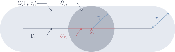
Figure 2: Sketch of the domains of analyticity of various functions used in the analycitity proof. The mapping $\psi_{t}$ of Theorem 5.14 is defined on $\Gamma_{i}$ (grey horizontal line) and is $\mathbb{R}$-analytic on the interval $U_{\tau_{i}}\subset\Gamma_{i}$ of the real line (red). We use partial derivatives $\partial^{k}_{y}u$ defined on $\Gamma_{i}\subset\mathbb{R}$, and the bounds of Theorem 5.11 to define Fréchet derivatives in an appropriate Banach space and obtain analyticity of $\psi_{t}$ on $U_{\tau_{i}}$. The function $\tilde{\psi}_{t}$ in the proof of Corollary 5.16 is defined on $\mathbb{C}$ and is $\mathbb{C}$-analytic in $\tilde{U}_{\tau_{i}}$ (dark grey). Without upgrading our definition of derivatives we prove that $\tilde{\psi}_{t}$ is the analytic extension of $\psi_{t}$ on $\tilde{U}_{\tau_{i}}$. Finally, we prove the existence of a function $\tilde{u}_{n}$ that extends $\psi_{t}$ analytically in the whole $\Sigma(\Gamma_{i},\tau_{i})$ (light grey).

in conjunction with bound Eq. 22 of Theorem 5.11. We therefore know that $m_{k}$ is a symmetric operator in $\mathcal{M}^{k}(\Gamma_{i},\mathbb{B})$, the set of $k$-linear operators on $\Gamma_{i}^{k}$ to $\mathbb{B}$ [16, Proposition 4.1.2] and by Eq. 33 we have, for almost every $y\in\Gamma_{i}$,

$$\psi_{t}(y)-\sum_{j=0}^{k}m_{j}(y-y_{0})^{j}=R_{k}(y_{0},y,t,{\mkern 2.0mu\cdot\mkern 2.0mu})\in\mathbb{B}.$$

We will now show that the sequence $\{R_{k}\}$ converges in $\mathbb{B}$ as $k\to\infty$. As an intermediate step, we bound $R_{k}$ in the $\mathbb{X}$-norm using the Taylor’s theorem bound for real-valued functions of a single variable, obtaining

$$\big{\|}R_{k}(y_{0},y,t,y_{i}^{*})\big{\|}_{\mathbb{X}}\leq\frac{|y-y_{0}|^{k+1}}{(k+1)!}\sup_{s\in[y_{0},y]}\|\partial_{y_{i}}^{k+1}u(t,s,y_{i}^{*})\|_{\mathbb{X}}$$

With the view of bounding $R_{k}$ in the $\mathbb{B}$-norm, we multiply each side of the previous inequality by the strictly positive number $\tilde{\sigma}_{i}(y_{0},y)=\{\min\sigma_{i}(s)\colon s\in[y_{0},y]\}$, and obtain

$$\tilde{\sigma}_{i}(y_{0},y)\big{\|}R_{k}(y_{0},y,t,y_{i}^{*})\big{\|}_{\mathbb{X}} \leq\frac{|y-y_{0}|^{k+1}}{(k+1)!}\tilde{\sigma}_{i}(y_{0},y)\sup_{s\in[y_{0},y]}\|\partial_{y_{i}}^{k+1}u(t,s,y_{i}^{*})\|_{\mathbb{X}}$$

$$\leq\frac{|y-y_{0}|^{k+1}}{(k+1)!}\sup_{s\in[y_{0},y]}\sigma_{i}(s)\|\partial_{y_{i}}^{k+1}u(t,s,y_{i}^{*})\|_{\mathbb{X}},$$

hence, by Theorem 5.11,

$$\big{\|}R_{k}(y_{0},y,t,{\mkern 2.0mu\cdot\mkern 2.0mu})\big{\|}_{\mathbb{B}} \leq\frac{1}{\tilde{\sigma}_{i}(y_{0},y)}\frac{|y-y_{0}|^{k+1}}{(k+1)!}\sup_{s^{\prime}\in\Gamma_{i}^{*}}\sigma_{i}^{*}(s^{\prime})\sup_{s\in[y_{0},y]}\sigma_{i}(s)\|\partial_{y_{i}}^{k+1}u(t,s,s^{\prime})\|_{\mathbb{X}}$$

$$\leq\frac{1}{\tilde{\sigma}_{i}(y_{0},y)}\frac{|y-y_{0}|^{k+1}}{(k+1)!}\sup_{s^{\prime}\in\Gamma_{i}^{*}}\sup_{s\in\Gamma_{i}}\sigma_{i}^{*}(s^{\prime})\sigma_{i}(s)\|\partial_{y_{i}}^{k+1}u(t,s,s^{\prime})\|_{\mathbb{X}}$$

$$\leq\frac{\bigl{(}|y-y_{0}|\delta_{i}(t)\bigr{)}^{k+1}}{\tilde{\sigma}(y_{0},y)}\|D_{i}(t,{\mkern 2.0mu\cdot\mkern 2.0mu})\|_{C^{0}_{\sigma}(\Gamma)}.$$

We can now draw a few conclusions: firstly, owing to the previous inequality, the power series

$$\psi_{t}(y)=\sum_{j=0}^{\infty}m_{j}(y-y_{0})^{j}$$

converges for all $y$ in the interval $U_{\tau_{i}}=\{|y-y_{0}|\leq\tau_{i}\}\subset\Gamma_{i}$, with $0<\tau_{i}<1/\delta_{i}(t)$. Secondly, we return to the estimate Eq. 34, which gives

$$\sup_{k\geq 0}\tau_{i}^{k}\|m_{k}\|<\infty,\qquad 0<\tau_{i}<\delta_{i}(t).$$

The hypotheses of [16, Proposition 4.3.4] are verified and we conclude that for any $0<\tau<\delta_{i}(t)$: (i) the mapping $\psi_{t}$ is $\mathbb{R}$-analytic on $U_{\tau_{i}}$ [16, Definition 4.3.1]; (ii) it holds $\psi_{t}\in C^{\infty}(U_{\tau_{i}},\mathbb{B})$; and (iii) $m_{k}$ is the $k$th Fréchet derivative $d^{k}\psi_{t}[y_{0}]$ of $\psi_{t}$ at $y_{0}\in U_{\tau_{i}}$. The proof is now complete.

We have proved $\mathbb{R}$-analyticity of the $C^{0}_{\sigma_{i}}(\Gamma_{i},\mathbb{X})$-valued solution $y_{i}\mapsto u_{n}(t,y_{i},{\mkern 2.0mu\cdot\mkern 2.0mu})$ on an interval in $\Gamma_{i}\subset\mathbb{R}$. To that effect, we transplanted bounds on partial derivatives of the real-valued solution $\partial_{y_{i}}^{k}u_{n}$, to bounds on the Fréchet derivative of the mapping above. We now extend this $\mathbb{R}$-analytic mapping to a $\mathbb{C}$-analytic mapping, defined on an open set of the complex plane. Importantly, this extension can be carried out without investigating Fréchet differentiability of Banach-space valued functions of complex variables, on the field $\mathbb{C}$, for which we have thus far proved no result.

Corollary 5.16 (to Theorem 5.14; $\mathbb{C}$-analytic extension of the projmected solution with values in $\mathbb{X}$).

Assume the hypothesis of Theorem 5.11, fix $n,m\in\mathbb{N}$, $i\in\mathbb{N}_{m}$ and $t\in J$. The solution of the projected problem $u_{n}(t,y_{i},y_{i}^{*})$ as an $\mathbb{R}$-analytic function of $y_{i}$, $u_{n}\colon\Gamma_{i}\subseteq\mathbb{R}\to C^{0}_{\sigma^{*}_{i}}(\Gamma_{i}^{*},\mathbb{X})$ admits a $\mathbb{C}$-analytic extension $\tilde{u}_{n}\colon\mathbb{C}\to C^{0}_{\sigma^{*}_{i}}(\Gamma_{i}^{*},\mathbb{X})$ in the region of the complex plane

$$\Sigma(\Gamma_{i},\tau_{i})=\{z\in\mathbb{C}:\operatorname{dist}(\Gamma_{i},z)\leq\tau_{i}\},$$

for any $0<\tau_{i}<1/\delta_{i}(t)$.

Proof 5.17.

Pick $y_{0}\in\Gamma_{i}$, and let $\mathbb{B}_{\mathbb{C}}$ be the Banach space $C^{0}_{\sigma^{*}_{i}}(\Gamma_{i}^{*},\mathbb{X})$ on the field $\mathbb{C}$. Introduce the mappings

(35) $$\tilde{\psi}_{k}\colon\mathbb{C}\to\mathbb{B}_{\mathbb{C}},\qquad z\mapsto\sum_{j=0}^{k}\frac{1}{j!}\partial_{y_{i}}^{j}u_{n}(t,y_{0},{\mkern 2.0mu\cdot\mkern 2.0mu})(z-y_{0})^{j}\qquad k\geq 1.$$

In passing we note that $\tilde{\psi}_{k}$ defined above and $\psi_{t}$ in Theorem 5.14 have different domains (a subset of $\mathbb{C}$ and $\mathbb{R}$, respectively) but also different codomains: the former has values in $\mathbb{B}_{\mathbb{C}}$, and the latter in $\mathbb{B}$, that is $C^{0}_{\sigma^{*}_{i}}(\Gamma_{i}^{*},\mathbb{X})$ on the field $\mathbb{R}$.

Proceeding as in the proof of Theorem 5.14, and replacing the absolute value $|{\mkern 2.0mu\cdot\mkern 2.0mu}|_{\mathbb{R}}$ appearing in the $\mathbb{X}$ norms by the absolute value $|{\mkern 2.0mu\cdot\mkern 2.0mu}|_{\mathbb{C}}$, we bound $\|\partial_{y_{i}}^{j}u_{n}(t,y_{0},{\mkern 2.0mu\cdot\mkern 2.0mu})(z-y_{0})^{j}/j!\|_{\mathbb{B}_{\mathbb{C}}}$, and find

$$\lim_{k\to\infty}\tilde{\psi}_{k}(z)\to\tilde{\psi}_{t}(z)\qquad\text{as $k\to\infty$}\qquad\text{for all $z\in\tilde{U}_{\tau_{i}}$}$$

for some $\mathbb{B}_{\mathbb{C}}$-valued function $\tilde{\psi}_{t}$, where $\tilde{U}_{\tau_{i}}=\{z\in\mathbb{C}\colon|z-y_{0}|\leq\tau_{i}\}$, with $0<\tau_{i}<1/\delta_{i}(t)$.

For any $0<\tau_{i}<\delta_{i}(t)$, Theorem 5.14 defines $\psi_{t}$, a $\mathbb{B}$-valued function that is $\mathbb{R}$-analytic in $U_{\tau_{i}}\subset\tilde{U}_{\tau_{i}}$. Above we proved the existence of $\tilde{\psi}_{t}$, a $\mathbb{B}_{\mathbb{C}}$-valued function that is $\mathbb{C}$-analytic in $\tilde{U}_{\tau_{i}}$ and such that

$$\tilde{\psi}_{t}(y)=\sum_{k=0}^{\infty}\frac{1}{k!}d^{k}\psi[y_{0}](y-y_{0})^{k}=\psi_{t}(y)=u_{n}(t,y,{\mkern 2.0mu\cdot\mkern 2.0mu})\qquad\text{for all $y\in U_{\tau_{i}}$}.$$

We therefore found an analytic extension to the solution $u_{n}$ in $\tilde{U}_{\tau_{i}}$. The steps above can be repeated for any $y_{0}\in\Gamma_{i}$, providing an extension $\tilde{u}_{n}$ to $u_{n}$ in $\Sigma(\Gamma,\tau_{i})$ for all $0<\tau_{i}<1/\delta_{i}(t)$.

The results of Theorems 5.14 and 5.16 concern analyticity of the time-dependent function $u_{n}(t,{\mkern 2.0mu\cdot\mkern 2.0mu})$. Theorem 5.11 also provides Eq. 23, a bound valid for $t\in J=[0,T]$, and it is possible to obtain analyticity of $u_{n}$ as a $C^{0}(J,\mathbb{X})$-valued solution, as the following result shows. [$\mathbb{C}$-analyticity of the semidiscrete solution with values in $C^{0}(J,\mathbb{X})$] Assume the hypotheses of Theorem 5.11, and fix $n\in\mathbb{N}$ and $i\in\mathbb{N}_{m}$. The solution of the projected problem $u_{n}({\mkern 2.0mu\cdot\mkern 2.0mu},y_{i},y_{i}^{*})$ as an $\mathbb{R}$-analytic function of $y_{i}$, $u_{n}\colon\Gamma_{i}\subseteq\mathbb{R}\to C^{0}_{\sigma^{*}_{i}}(\Gamma_{i}^{*},C^{0}(J,\mathbb{X}))$ admits a $\mathbb{C}$-analytic extension $\tilde{u}_{n}\colon\mathbb{C}\to C^{0}_{\sigma^{*}_{i}}(\Gamma_{i}^{*},C^{0}(J,\mathbb{X}))$ in the region of the complex plane

$$\Sigma(\Gamma_{i},\tau_{i})=\{z\in\mathbb{C}:\operatorname{dist}(\Gamma_{i},z)\leq\tau_{i}\},$$

for any $0<\tau_{i}<1/\|\delta_{i}\|_{C^{0}(J)}$. The proof is a straightforward amendment of the ones in Theorems 5.14 and 5.16. We amend the definition of $\mathbb{B}$ as $\mathbb{B}=C^{0}_{\sigma_{i}^{*}}(\Gamma_{i}^{*},C^{0}(J,\mathbb{X}))$ over $\mathbb{R}$, and let

$$\psi\colon\Gamma_{i}\subset\mathbb{R}\to\mathbb{B},\qquad y_{i}\mapsto u_{n}({\mkern 2.0mu\cdot\mkern 2.0mu},y_{i},{\mkern 2.0mu\cdot\mkern 2.0mu}).$$

From Eq. 33 we derive

$$\psi(y)-\sum_{j=0}^{k}m_{j}(y-y_{0})^{j}=R_{k}(y_{0},y,{\mkern 2.0mu\cdot\mkern 2.0mu},{\mkern 2.0mu\cdot\mkern 2.0mu})\in\mathbb{B},$$

with the updated definitions $m_{0}(y-y_{0})^{0}=\psi(y_{0})$, and

$$m_{k}\colon(\gamma_{1},\ldots,\gamma_{k})\mapsto\frac{1}{k!}\partial_{y_{i}}^{k}u_{n}({\mkern 2.0mu\cdot\mkern 2.0mu},y_{0},{\mkern 2.0mu\cdot\mkern 2.0mu})\gamma_{1}\cdots\gamma_{k},\qquad k\geq 1,$$

whose norm is bounded using Eq. 23 and proceeding as in (34)

$$\|m_{k}\|\leq\frac{1}{k!\sigma_{i}(y_{0})}\|\partial_{y_{i}}^{k}u_{n}\|_{C^{0}_{\sigma}(\Gamma,C^{0}(J,\mathbb{X}))}\leq\frac{1}{\sigma_{i}(y_{0})}\|\delta_{i}\|^{k}_{C^{0}(J)}\|D_{i}\|_{C^{0}_{\sigma}(\Gamma,C^{0}(J))}<\infty.$$

The operator $m_{k}$ is symmetric and in $\mathcal{M}^{k}(\Gamma_{i},\mathbb{B})$, [16, Proposition 4.1.2]. Proceeding as in the proof of Theorem 5.14, we introduce $\tilde{\sigma}_{i}(y_{0},y)=\{\min\sigma_{i}(s)\colon s\in[y_{0},y]\}$ and estimate

$$\big{\|}R_{k}(y_{0},y,{\mkern 2.0mu\cdot\mkern 2.0mu},{\mkern 2.0mu\cdot\mkern 2.0mu})\big{\|}_{\mathbb{B}} \leq\frac{1}{\tilde{\sigma}_{i}(y_{0},y)}\frac{|y-y_{0}|^{k+1}}{(k+1)!}\sup_{s^{\prime}\in\Gamma_{i}^{*}}\sup_{s\in\Gamma_{i}}\sigma_{i}^{*}(s^{\prime})\sigma_{i}(s)\|\partial_{y_{i}}^{k+1}u({\mkern 2.0mu\cdot\mkern 2.0mu},s,s^{\prime})\|_{C^{0}(J,\mathbb{X})}$$

$$\leq\frac{\bigl{(}|y-y_{0}|\,\|\delta_{i}\|_{C^{0}(J)}\bigr{)}^{k+1}}{\tilde{\sigma}(y_{0},y)}\|D_{i}\|_{C^{0}_{\sigma}(\Gamma,C^{0}(J))}$$

hence the power series $\psi(y)=\sum_{j=0}^{\infty}m_{j}(y-y_{0})^{j}$ converges for all $y$ in the interval $U_{\tau_{i}}=\{|y-y_{0}|\leq\tau_{i}\}$ with $0<\tau_{i}<1/\|\delta_{i}\|_{C^{0}(J)}$, the following bound holds

$$\sup_{k\geq 0}\tau_{i}^{k}\|m_{k}\|<\infty,\qquad 0<\tau_{i}<1/\|\delta_{i}\|_{C^{0}(J)},$$

and by [16, Proposition 4.3.4] the mapping $\psi\colon\Gamma_{i}\to\mathbb{B}$ is $\mathbb{R}$-analytic on $U_{\tau_{i}}$ [16, Definition 4.3.1] with

$$d^{k}\psi_{t}[y_{0}]\colon\Gamma_{i}^{k}\subset\mathbb{R}^{k}\to C^{0}_{\sigma_{i}^{*}}(\Gamma_{i}^{*},C^{0}(J,\mathbb{X}))\qquad(\gamma_{1},\ldots,\gamma_{k})\mapsto\partial_{y_{i}}^{k}u_{n}({\mkern 2.0mu\cdot\mkern 2.0mu},y_{0},{\mkern 2.0mu\cdot\mkern 2.0mu})\gamma_{1}\cdots\gamma_{k}.$$

The existence of an analytic extension $\tilde{u}_{n}$ to $u_{n}$ follows steps identical to the ones in Corollary 5.16, upon setting $\mathbb{B}_{C}=C^{0}_{\sigma^{*}_{i}}(\Gamma^{*}_{i},C^{0}(J,\mathbb{X}))$ on the field $\mathbb{C}$, amending the sequence $\{\tilde{\psi}_{k}\}$

(36) $$\tilde{\psi}_{k}\colon\mathbb{C}\to\mathbb{B}_{\mathbb{C}},\qquad z\mapsto\sum_{j=0}^{k}\frac{1}{j!}\partial_{y_{i}}^{j}u_{n}({\mkern 2.0mu\cdot\mkern 2.0mu},y_{0},{\mkern 2.0mu\cdot\mkern 2.0mu})(z-y_{0})^{j}\qquad k\geq 1,$$

and replacing $\delta_{i}(t)$ by $\|\delta_{i}\|_{C^{0}(J)}$.

5.5 Error estimate for the spatial projection, stochastic collocation scheme

We are ready to give an a priori estimate for the stochastic collocation scheme’s total error. We use results in [12] for PDEs with random data, as the estimates for the interpolation in the $y$ direction do not depend on the particular problem but only rely on analyticity of the data and solution, and we combine it with the theory developed in [6] for neural fields.

Theorem 5.18 (Total error bound).

Assume the hypotheses of Theorem 5.11, and Section 5 (sub-Gaussianity). There exist positive constants $C_{\textnormal{sc}},r_{1},\ldots,r_{m}$ independent of $n$ and $q$, such that, for all $t\in J$ it holds

(37) $$\|u(t,{\mkern 2.0mu\cdot\mkern 2.0mu})-u_{n,q}(t,{\mkern 2.0mu\cdot\mkern 2.0mu})\|_{L^{2}_{\rho}(\Gamma)\otimes\mathbb{X}} \leq\|u-u_{n,q}\|_{L^{2}_{\rho}(\Gamma)\otimes C^{0}(J,\mathbb{X})}$$

$$\leq e^{\bar{K}_{w}T}\|u-P_{n}u\|_{L^{2}_{\rho}(\Gamma)\otimes C^{0}(J,\mathbb{X})}+C_{\textnormal{sc}}\sum_{i=1}^{m}\beta_{i}(q_{i})\,e^{-r_{i}q_{i}^{\theta_{i}}},$$

where, if $\Gamma_{i}$ is bounded

$$r_{i}=\log\left[\frac{2\tau_{i}}{|\Gamma|}\left(1+\sqrt{1+\frac{|\Gamma_{i}|^{2}}{4\tau_{i}^{2}}}\right)\right],\qquad\theta_{i}=\beta_{i}=1,$$

and if $\Gamma_{i}$ is unbounded

$$r_{i}=\tau_{i}\zeta_{i},\qquad\theta_{i}=\frac{1}{2},\qquad\beta_{i}\in O(\sqrt{q_{i}})\text{ as $q_{i}\to\infty$},$$

$\bar{K}_{w}$ being defined in Remark 5.3, $\tau_{i}$ in 5.17, and $\zeta_{i}$ in Section 5.

Proof 5.19.

To prove the first inequality we note that, if $f$ is a function in $L^{2}_{\rho}(\Gamma,C^{0}(J,\mathbb{X}))$ then for all $t\in J$ it holds

$$\|f(t,{\mkern 2.0mu\cdot\mkern 2.0mu})\|^{2}_{L^{2}_{\rho}(\Gamma)\otimes\mathbb{X}}=\int_{\Gamma}\|f(t,y)\|_{\mathbb{X}}^{2}\,\rho(y)\,dy\leq\int_{\Gamma}\|f({\mkern 2.0mu\cdot\mkern 2.0mu},y)\|_{C^{0}(J,\mathbb{X})}^{2}\,\rho(y)\,dy=\|f\|_{L^{2}_{\rho}(\Gamma)\otimes C^{0}(J,\mathbb{X})}^{2},$$

hence we proceed to verify that $u,u_{nq}\in L^{2}_{\rho}(\Gamma,C^{0}(J,\mathbb{X}))$ and infer

(38) $$\|u(t,{\mkern 2.0mu\cdot\mkern 2.0mu})-u_{n,q}(t,{\mkern 2.0mu\cdot\mkern 2.0mu})\|_{L^{2}_{\rho}(\Gamma)\otimes\mathbb{X}}\leq\|u-u_{n,q}\|_{L^{2}_{\rho}(\Gamma)\otimes C^{0}(J,\mathbb{X})}\qquad t\in J.$$

Since the hypotheses of [9, Corollary 6.2 with $p=2$] hold we have $u,u_{n}\in L^{2}_{\rho}(\Gamma,C^{0}(J,\mathbb{X}))$. Further, by Lemma 5.5 $u_{n}\in C^{0}_{\sigma}(\Gamma,C^{0}(J,\mathbb{X}))$ and the sub-Gaussianity hypothesis (Section 5) guarantees that the embedding $C^{0}_{\sigma}(\Gamma,C^{0}(J,\mathbb{X}))\subset L^{2}_{\rho}(\Gamma,C^{0}(J,\mathbb{X}))$ is continuous (see [12, page 1019, discussion preceeding Lemma 4.2]). We recall that $u_{n,q}(x,t,y)=(I_{q}u_{n}(x,t,{\mkern 2.0mu\cdot\mkern 2.0mu})(y)$ by definition Eq. 14, thus we interpret $I_{q}$ as an operator on $C^{0}_{\sigma}(\Gamma,C^{0}(J,\mathbb{X}))$ to $L^{2}_{\rho}(\Gamma,C^{0}(J,\mathbb{X}))$ and by [12, Lemma 4.3 and its proof taking $V=C^{0}(J,\mathbb{X})$] there exists a constant $C_{q}$ such that

$$\|u_{n,q}\|_{L^{2}_{\rho}(\Gamma,C^{0}(J,\mathbb{X}))}=\|I_{q}u_{n}\|_{L^{2}_{\rho}(\Gamma,C^{0}(J,\mathbb{X}))}\leq C_{q}\|u_{n}\|_{C^{0}_{\sigma}(\Gamma,C^{0}(J,\mathbb{X}))}<\infty.$$

We have thus verified $u,u_{n,q}\in L^{2}_{\rho}(\Gamma,C^{0}(J,\mathbb{X}))$, hence (38) holds. By the triangle inequality

$$\|u-u_{n,q}\|_{L^{2}_{\rho}(\Gamma)\otimes C^{0}(J,\mathbb{X})}\leq\|u-u_{n}\|_{L^{2}_{\rho}(\Gamma)\otimes C^{0}(J,\mathbb{X})}+\|u_{n}-u_{n,q}\|_{L^{2}_{\rho}(\Gamma)\otimes C^{0}(J,\mathbb{X})}=:I+II.$$

Using Section 4.1 and Remark 5.3 for $k=0$ we estimate the spatial discretisation error

$$I^{2} =\int_{\Gamma}\|u({\mkern 2.0mu\cdot\mkern 2.0mu},y)-u_{n}({\mkern 2.0mu\cdot\mkern 2.0mu},y)\|_{C^{0}(J,\mathbb{X})}^{2}\rho(y)\,dy$$

$$\leq\int_{\Gamma}\bigl{(}e^{T\|P_{n}W(y)\|}\bigr{)}^{2}\|u(t,y)-P_{n}u(t,y)\|^{2}_{\mathbb{X}}\,\rho(y)\,dy\leq\bigl{(}e^{T\bar{K}_{w}}\bigr{)}^{2}\|u-P_{n}u\|^{2}_{L^{2}_{\rho}(\Gamma,C^{0}(J,\mathbb{X}))},$$

which gives the first term on the right-hand side of Eq. 37. For the stochastic collocation error the following estimate holds

$$II\leq C_{\textrm{sc}}\sum_{i=1}^{m}\beta_{i}(q_{i})\,e^{-r_{i}q_{i}^{\theta_{i}}}.$$

with constants given in the theorem statement. This estimate follows identical steps to the proof of Theorem 4.1 in [12, page 1024], except that: (i) it is carried out for $u_{n}$, not $u$; (ii) it involves functions with values in the Banach space $V=C^{0}(J,\mathbb{X})$, and (iii) it uses the analyticity result in 5.17. We omit the details of the proof of this bound for brevity, and we stress that, with respect to [12], we have different radii of analyticity $\tau_{i}$, and we treat simultaneously the Banach spaces $\mathbb{X}\in\{C(D),L^{2}(D)\}$, but the proof steps are unchanged.

The bound in Theorem 5.18 is useful also as an upper bound on the first and second moments of the error, as we can use the upcoming 5.19 with $v=u$ and $z=u_{n,q}$. 5.19 is an adaptation of [12, Lemmas 4.7 and 4.8] to the problem under consideration.

[Errors for first and second moments] If $v,z\in L^{2}_{\rho}(\Gamma,\mathbb{X})$, then

(39) $$\bigl{\|}\operatorname{\mathbb{E}}_{\rho}(v-z)\bigr{\|}_{\mathbb{X}}\leq\|v-z\|_{L^{2}_{\rho}(\Gamma)\otimes\mathbb{X}},$$

(40) $$\|\operatorname{\mathbb{E}}_{\rho}(v^{2}-z^{2})\|_{\mathbb{X}}\leq\|v+z\|_{L^{2}_{\rho}(\Gamma)\otimes\mathbb{X}}\|v-z\|_{L^{2}_{\rho}(\Gamma)\otimes\mathbb{X}}, \mathbb{X}=C(D)$$

(41) $$\|\operatorname{\mathbb{E}}_{\rho}(v^{2}-z^{2})\|_{L^{1}(D)}\leq\|v+z\|_{L^{2}_{\rho}(\Gamma)\otimes\mathbb{X}}\|v-z\|_{L^{2}_{\rho}(\Gamma)\otimes\mathbb{X}}, \mathbb{X}=L^{2}(D),$$

whereas, if $v,z\in L^{2}_{\rho}(\Gamma,C^{0}(J,\mathbb{X}))$, then

(42) $$\bigl{\|}\operatorname{\mathbb{E}}_{\rho}(v-z)\bigr{\|}_{C^{0}(J,\mathbb{X})}\leq\|v-z\|_{L^{2}_{\rho}(\Gamma)\otimes C^{0}(J,\mathbb{X})},$$

(43) $$\|\operatorname{\mathbb{E}}_{\rho}(v^{2}-z^{2})\|_{C^{0}(J,\mathbb{X})}\leq\|v+z\|_{L^{2}_{\rho}(\Gamma)\otimes C^{0}(J,\mathbb{X})}\|v-z\|_{L^{2}_{\rho}(\Gamma)\otimes C^{0}(J,\mathbb{X})}, \mathbb{X}=C(D)$$

(44) $$\|\operatorname{\mathbb{E}}_{\rho}(v^{2}-z^{2})\|_{C^{0}(J,L^{1}(D))}\leq\|v+z\|_{L^{2}_{\rho}(\Gamma)\otimes C^{0}(J,\mathbb{X})}\|v-z\|_{L^{2}_{\rho}(\Gamma)\otimes C^{0}(J,\mathbb{X})}, \mathbb{X}=L^{2}(D),$$

If $\mathbb{X}=C(D)$, then Eq. 39 is derived using Hölder’s inequality on $f=v-z$, as follows

$$\|\operatorname{\mathbb{E}}_{\rho}f\|_{\mathbb{X}} =\sup_{x\in D}\biggl{|}\int_{\Gamma}f(x,y)\rho(y)\,dy\biggr{|}\leq\sup_{x\in D}\int_{\Gamma}|f(x,y)|\rho(y)\,dy$$

$$\leq\int_{\Gamma}\|f({\mkern 2.0mu\cdot\mkern 2.0mu},y)\|_{\mathbb{X}}1_{\Gamma}(y)\rho(y)\,dy\leq\biggl{[}\int_{\Gamma}\|f({\mkern 2.0mu\cdot\mkern 2.0mu},y)\|^{2}_{\mathbb{X}}\rho(y)\,dy\biggr{]}^{1/2}\biggl{[}\int_{\Gamma}1_{\Gamma}(y)\rho(y)\,dy\biggr{]}^{1/2}$$

$$=\|f\|_{L^{2}_{\rho}(\Gamma,\mathbb{X})},$$

whereas for $\mathbb{X}=L^{2}(D)$ the bound Eq. 39 is found via the estimate (see also [55, page 1934]),

$$\|\operatorname{\mathbb{E}}_{\rho}f\|^{2}_{\mathbb{X}} =\int_{D}\biggl{|}\int_{\Gamma}f(x,y)\rho(y)\,dy\biggr{|}^{2}\,dx=\int_{D}\bigl{\langle}f(x,{\mkern 2.0mu\cdot\mkern 2.0mu}),1_{\Gamma}\bigr{\rangle}^{2}_{\rho}\,dx$$

$$\leq\biggl{[}\int_{D}\|f(x,{\mkern 2.0mu\cdot\mkern 2.0mu})\|^{2}_{L^{2}(\Gamma)}\rho(y)\,dy\biggr{]}\biggr{[}\int_{D}\rho(y)\,dy\biggl{]}=\int_{\Gamma}\int_{D}|f(x,y)|^{2}\rho(y)\,dx\,dy=\|f\|^{2}_{L^{2}_{\rho}(\Gamma)\otimes\mathbb{X}}.$$

To prove Eq. 40 we set $\mathbb{X}\in C(D)$ and derive

$$\|E_{\rho}(v^{2}-z^{2})\|_{\mathbb{X}} =\sup_{x\in D}\int_{\Gamma}|v(x,y)+z(x,y)|\,|v(x,y)-z(x,y)|\rho(y)\,dy$$

$$\leq\int_{\Gamma}\|v({\mkern 2.0mu\cdot\mkern 2.0mu},y)+z({\mkern 2.0mu\cdot\mkern 2.0mu},y)\|_{\mathbb{X}}\,\|v({\mkern 2.0mu\cdot\mkern 2.0mu},y)-z({\mkern 2.0mu\cdot\mkern 2.0mu},y)\|_{\mathbb{X}}\rho(y)\,dy$$

$$\leq\biggl{[}\int_{\Gamma}\|v({\mkern 2.0mu\cdot\mkern 2.0mu},y)+z({\mkern 2.0mu\cdot\mkern 2.0mu},y)\|_{\mathbb{X}}\rho(y)\,dy\biggr{]}^{1/2}\biggl{[}\int_{\Gamma}\|v({\mkern 2.0mu\cdot\mkern 2.0mu},y)-z({\mkern 2.0mu\cdot\mkern 2.0mu},y)\|_{\mathbb{X}}\rho(y)\,dy\biggr{]}^{1/2}$$

$$\leq\|v+z\|_{L^{2}_{\rho}(\Gamma)\otimes\mathbb{X}}\|v-z\|_{L^{2}_{\rho}(\Gamma)\otimes\mathbb{X}},$$

whereas the bound Eq. 41 is proved in [12, Lemma 4.8]. To prove bounds in the $\|{\mkern 2.0mu\cdot\mkern 2.0mu}\|_{C^{0}(J,\mathbb{X})}$ norm it is useful to note that, if $f\in L^{2}_{\rho}(\Gamma,C^{0}(J,\mathbb{X}))$, then for all $t\in J$ it holds

$$\|f(t,{\mkern 2.0mu\cdot\mkern 2.0mu})\|^{2}_{L^{2}_{\rho}(\Gamma)\otimes\mathbb{X}}=\int_{\Gamma}\|f(t,y)\|_{\mathbb{X}}^{2}\,\rho(y)\,dy\leq\int_{\Gamma}\|f({\mkern 2.0mu\cdot\mkern 2.0mu},y)\|_{C^{0}(J,\mathbb{X})}^{2}\,\rho(y)\,dy=\|f\|_{L^{2}_{\rho}(\Gamma)\otimes C^{0}(J,\mathbb{X})}^{2}.$$

Combining this bound with Eq. 39 we derive Eq. 42 jointly for $\mathbb{X}\in\{C(D),L^{2}(D)\}$,

$$\|\operatorname{\mathbb{E}}_{\rho}v\|_{C^{0}(J,\mathbb{X})}=\sup_{t\in J}\|\operatorname{\mathbb{E}}_{\rho}v(t,{\mkern 2.0mu\cdot\mkern 2.0mu})\|_{\mathbb{X}}\leq\sup_{t\in J}\|v(t,{\mkern 2.0mu\cdot\mkern 2.0mu})\|_{L^{2}_{\rho}(\Gamma)\otimes\mathbb{X}}\leq\|v\|_{L^{2}_{\rho}(\Gamma)\otimes C^{0}(J,\mathbb{X})}.$$

Equation 43 is derived using Eq. 40 and the property derived above for $f\in L^{2}_{\rho}(\Gamma,C^{0}(J,\mathbb{X}))$,

$$\|E_{\rho}(v^{2}-z^{2})\|_{C^{0}(J,\mathbb{X})} \leq\sup_{t\in J}\bigl{\|}E_{\rho}\bigl{[}v^{2}(t,{\mkern 2.0mu\cdot\mkern 2.0mu})-z^{2}(t,{\mkern 2.0mu\cdot\mkern 2.0mu})\bigr{]}\bigr{\|}_{\mathbb{X}}$$

$$\leq\sup_{t\in J}\biggl{[}\|v(t,{\mkern 2.0mu\cdot\mkern 2.0mu})+z(t,{\mkern 2.0mu\cdot\mkern 2.0mu})\|_{L^{2}_{\rho}(\Gamma)\otimes\mathbb{X}}\,\|v(t,{\mkern 2.0mu\cdot\mkern 2.0mu})-z(t,{\mkern 2.0mu\cdot\mkern 2.0mu})\|_{L^{2}_{\rho}(\Gamma)\otimes\mathbb{X}}\biggr{]}$$

$$\leq\|v+z\|_{L^{2}_{\rho}(\Gamma)\otimes C^{0}(J,\mathbb{X})}\,\|v-z\|_{L^{2}_{\rho}(\Gamma)\otimes C^{0}(J,\mathbb{X})},$$

and similarly Eq. 44 is a consequence of Eq. 41

$$\|E_{\rho}(v^{2}-z^{2})\|_{C^{0}(J,L^{1}(D))} \leq\sup_{t\in J}\bigl{\|}E_{\rho}\bigl{[}v^{2}(t,{\mkern 2.0mu\cdot\mkern 2.0mu})-z^{2}(t,{\mkern 2.0mu\cdot\mkern 2.0mu})\bigr{]}\bigr{\|}_{L^{1}(D)}$$

$$\leq\sup_{t\in J}\biggl{[}\|v(t,{\mkern 2.0mu\cdot\mkern 2.0mu})+z(t,{\mkern 2.0mu\cdot\mkern 2.0mu})\|_{L^{2}_{\rho}(\Gamma)\otimes\mathbb{X}}\,\|v(t,{\mkern 2.0mu\cdot\mkern 2.0mu})-z(t,{\mkern 2.0mu\cdot\mkern 2.0mu})\|_{L^{2}_{\rho}(\Gamma)\otimes\mathbb{X}}\biggr{]}$$

$$\leq\|v+z\|_{L^{2}_{\rho}(\Gamma)\otimes C^{0}(J,\mathbb{X})}\,\|v-z\|_{L^{2}_{\rho}(\Gamma)\otimes C^{0}(J,\mathbb{X})},$$

5.6 An example of estimating the total error bound using Theorem 5.18

We conclude this section by showing how to use Theorem 5.18 in a concrete example.

Example 5.20 (Example 5.7, continued).

Consider a RLNF with random data

(45) $$v(x,\omega_{v})=b_{0}(x)+\sum_{j\in\mathbb{N}_{m}}b_{j}(x)Y_{j}(\omega_{g}),\quad Y_{i}\stackrel{{\scriptstyle i.i.d}}{{\sim}}\mathcal{U}[-\alpha,\alpha],\quad i\in\mathbb{N}^{m},\quad x\in D=[-1,1],$$

in which the functions $\{b_{j}\}_{j}$ as well as the other, deterministic, neural field data $w$ and $g$ are chosen so that, for any fixed $y\in\Gamma_{v}=[-\alpha,\alpha]$ it holds $u({\mkern 2.0mu\cdot\mkern 2.0mu},{\mkern 2.0mu\cdot\mkern 2.0mu},y)\in C^{0}(J,C^{2}(D))$. Further assume the problem is discretise using a Finite-Element Collocation scheme, as in Example 5.7. The projections $P_{n}$ of this scheme is such that [4, Equation 2.3.48]

$$\|z-P_{n}z\|_{\infty}\leq\frac{|D|^{2}}{8n^{2}}\|v^{\prime\prime}\|_{\infty}=\frac{1}{2n^{2}}\|v^{\prime\prime}\|_{\infty},\qquad v\in C^{2}(D).$$

We now reason as follows: by [9, Corollaries 5.1 and 6.2] $u\in L^{2}_{\rho}(\Gamma_{v},C^{0}(J,\mathbb{X}))$ and $u_{n}\in L^{2}_{\rho}(\Gamma_{v},C^{0}(J,\mathbb{X}_{n}))$, respectively, with $\rho(y)\equiv(2\alpha)^{-1}$, $\mathbb{X}=\bigl{(}C^{0}(J,D),\|{\mkern 2.0mu\cdot\mkern 2.0mu}\|_{\infty}\bigr{)}$, and $\mathbb{X}_{n}$ as in Example 5.7. We now estimate

$$\|u-P_{n}u\|^{2}_{L^{2}_{\rho}(\Gamma)\otimes C^{0}(J,\mathbb{X})} =\int_{\Gamma}\biggl{[}\max_{(x,t)\in J\times D}\bigl{|}u(x,t,y)-(P_{n}u({\mkern 2.0mu\cdot\mkern 2.0mu},t,y))(x)\bigr{|}\biggr{]}^{2}\rho(y)\,dy$$

$$\leq\biggl{(}\frac{1}{2n^{2}}\biggr{)}^{2}\int_{\Gamma}\Biggl{[}\max_{t\in J}\biggl{\|}\frac{\partial^{2}u}{\partial x^{2}}({\mkern 2.0mu\cdot\mkern 2.0mu},t,y)\biggr{\|}\Biggr{]}^{2}\rho(y)\,dy$$

$$=\biggl{(}\frac{1}{2n^{2}}\biggr{)}^{2}\biggl{\|}\frac{\partial^{2}u}{\partial x^{2}}\biggr{\|}^{2}_{L^{2}_{\rho}(\Gamma,C^{0}(J,\mathbb{X}))}\leq\biggl{(}\frac{1}{2n^{2}}\biggr{)}^{2}\biggl{\|}\frac{\partial^{2}u}{\partial x^{2}}\biggr{\|}^{2}_{L^{2}_{\rho}(\Gamma,C^{0}(J,C^{2}(D)))}$$

We combine the estimate above with Eq. 42 in 5.19 and Eq. 37 in Theorem 5.18, use the fact that $\Gamma_{v}$ is bounded (hence $q_{i}=\theta_{i}=1$), and that the kernel $w$ is deterministic (hence we can take $\bar{K}_{w}=\|w\|_{\mathbb{W}}$) to arrive at

(46) $$\bigl{\|}\operatorname{\mathbb{E}}_{\rho}(u-u_{nq})\bigr{\|}_{C^{0}(J,\mathbb{X})}\leq C_{1}n^{-2}+C_{2}\sum_{i=1}^{m}e^{-r_{i}q_{i}},\qquad C_{1}=\frac{e^{T\|w\|_{\mathbb{W}}}}{2}\biggl{\|}\frac{\partial^{2}u}{\partial x^{2}}\biggr{\|}^{2}_{L^{2}_{\rho}(\Gamma,C^{0}(J,C^{2}(D)))}$$

and hence the error decays as an $O(n^{-2})$ as $n\to\infty$, and exponentially as $q_{i}\to\infty$, for any $i\in\mathbb{N}_{m}$.

6 Considerations on nonlinear neural fields

Section 5 discusses analyticity of solutions to the parametrised problem $u_{n}^{\prime}(t,y)=P_{n}N(t,u_{n}(t,y),y)$ with initial condition $u_{n}(0,y)=P_{n}v(y)$ when $\mathbb{L}=1$ (linear case). Under the boundedness assumption on the projectors $P_{n}$, Remark 5.4 ensures that the mapping $y_{i}\mapsto N({\mkern 2.0mu\cdot\mkern 2.0mu},{\mkern 2.0mu\cdot\mkern 2.0mu},(y_{i},y_{i}^{*}))$ is analytic, and Theorem 5.11 provides estimates determining the analyticity radius $\delta_{i}(t)$ of the mapping $y_{i}\to u_{n}({\mkern 2.0mu\cdot\mkern 2.0mu},y_{i},y_{i}^{*})$, in the appropriate function space.

A natural question arises as to how to adapt this approach in the nonlinear case ($\mathbb{L}=0$). The analyticity of solutions to generic Cauchy problems on Banach spaces is studied in [54, Theorem 4.11, Section 4.11, pages 165–166]. If the mapping $y\mapsto N({\mkern 2.0mu\cdot\mkern 2.0mu},{\mkern 2.0mu\cdot\mkern 2.0mu},y)$ is affine, conditions for analyticity of the solution are also given in [28]. With reference to the continuous parametrised problem

$$u^{\prime}(t,y)=N(t,u(t,y),y),\qquad(t,y)\in J\times\Gamma,\qquad u(0,y)=v(y)\qquad y\in\Gamma$$

we deduce that if $(t,u,y)\mapsto N(t,u,y)$ is analytic on $V\subseteq\mathbb{R}\times\mathbb{X}\times\Gamma$, then the mapping $(t,v,y)\mapsto u(t,v,y)$, in which we indicate dependence of the solution on the initial condition $v$, is analytic on an open $Z\subset V$.

If we pursued a study analogous to the linear case, however, appealing to such result would be insufficient, because bounding the total error as in Theorem 5.18 requires an estimate of the radius of analyticity $\tau$ (and this is precisely what Theorems 5.11 and 5.17 do for the linear case). We have also seen in Remarks 5.12 and 5.3.1 that, in the case of non-contracting dynamics, such radius shrinks as $t$ increases.

The dynamics of general nonlinear problems is deeply influenced by so-called bifurcation points. As a simple example, consider a family of equilibria of the neural field problem, $u_{*}(y_{i})$ which are in generically parametrised in one of the variables $y_{i}$. The dynamics of small perturbations to the rest state $u_{*}(y_{i})$ is governed by a linear problem, and the spectrum of the associated linear operators $A(y_{i})$ determines, roughly speaking, whether perturbations decay or grow. The spectrum of $A(y_{i})$ thus changes with the parameter value, and a frequent scenario in nonlinear problems is that the spectrum of $A(y_{i})$ crosses the imaginary axis as $y_{i}$ varies across a so-called bifurcation point, thereby determining a behavioural change in the solution, which may pass from a contracting to an expanding one, and vice versa.

In other words, in nonlinear problems the domains $\Gamma_{i}$ are generically enclosing bifurcation points, which mark sharp transitions in the mapping $y_{i}\mapsto u(t,y_{i})$ for $t$ fixed. Thus, in nonlinear problems the expectation is that $A(y_{i})$ will generally have eigenvalues on the right-half complex plane, for which we know that analyticity radii shrink as $t$ grows. Consequently, we can hope to observe numerically fast convergence rates on long time intervals only in cases where $\Gamma_{i}$ does not enclose bifurcations, with the spectrum of $A(y_{i})$ staying on the left-half complex plane for all $y_{i}\in\Gamma_{i}$.

We remark that these considerations are valid for generic nonlinear problems, not just the neural field presented here. In this paper, rather than pursuing the computation of analyticity radii for nonlinear projected problem, which seems possible and is expected to give shrinking analyticity radii, we employ stochastic collocation on nonlinear problems and present numerical evidence of convergence behaviour in Section 7.

7 Numerical results

We include in this section a collection of numerical experiments to test our scheme. All computations run on a laptop computer with 2 or 4 cores, except the convergence plots of Section 7.3, which were run on ADA, an HPC facility at VU Amsterdam, using 32 cores.

7.1 Problem 1: linear case, uniformly distributed parameter in $\mathbb{R}$

As first example we consider a linear neural field with one-dimensional, non-affine noise in the external input $g$. We choose a system that meets the hypotheses of Theorem 5.11 with $\mathbb{X}=C(D)$ (see Example 5.10 for checking analyticity of the random input), the sub-gaussianity hypothesis, and to which the theory of Section 5 for the error analysis applies. The problem’s solution and QOI are known in analytic form, allowing to compare theory and numerical experiments.

The neural field is posed on the spatio-temporal domain $J\times D=[0,T]\times[-L,L]$ with $T=L=1$, deterministic data

(47) $$w(x,x^{\prime})=xx^{\prime},\qquad f(x)=x,\qquad v(x)=\sin(4\pi x).$$

and a one-dimensional noise random input of the form $g(x,t,Y(\omega_{w}))$, with $Y\sim\mathcal{U}[\alpha,\beta]$ and

(48) $$g(x,t,y)=e^{ty}\Big{[}(y+1)\sin(4\pi x)+\frac{x}{2\pi}\Big{]},$$

for which the density $\rho(y)=(\beta-\alpha)^{-1}$ is defined on the compact $\Gamma_{g}=[\alpha,\beta]$, leading to

$$u(x,t,y)=e^{yt}\sin(4\pi x),\qquad\mathbb{E}_{\rho}[u(x,t,{\mkern 2.0mu\cdot\mkern 2.0mu})]=\frac{e^{\beta t}-e^{\alpha t}}{t(\beta-\alpha)}\sin(4\pi x),\qquad(x,t,y)\in D\times J\times\Gamma_{g}.$$

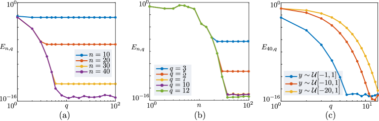
Figure 3: Spectral convergence of the stochastic colllocation method paired to Chebyshev collocation in space, for the RLNF problem with data Eqs. 47 to 48. (a) Error $E_{n,k}$, defined in Eq. 49 as a function of $q$, for various values of $n$, showing that the error decays expoentially until an $n$-dependent plateau, whose value is lower when $n$ increases. (b) Error $E_{n,k}$, as a function of $n$, for various values of $q$. (c) For fixed $n=40$ (which gives machine accuracy in the spatial error), the error $E_{40,q}$ is exponentially convergent and increases when the variance of the distribution $\mathcal{U}[\alpha,\beta]$ is larger. Parameters $T=1$, $L=1$ and, in (a,b), $\alpha=-2$, $\beta=0.5$.

The quantity of interest we approximate is the expectation of the spatial profile at final time, $\mathbb{E}_{\rho}[u(x,T,{\mkern 2.0mu\cdot\mkern 2.0mu})]$. The problem is discretised in space using a Chebyshev spectral collocation scheme with $n$ nodes, and Clenshaw-Curtis quadrature, which is spectrally convergent for fixed values of $y$ [6, 7]. For the time discretisation we used Matlab’s in-built, explicit, adaptive, 4th-order Runge-Kutta solver ode45. Our theory does not account for time-discretisation error (see [9] for an example of how this can be carried out in abstract form) and we set the relative and absolute tolerance to $10^{-14}$ and $10^{-15}$ respectively, so that spatial and stochastic collocation errors dominate the time-integration error. Integrals are computed using $q$ Gauss-Legendre quadrature with $q$ nodes on $\Gamma_{g}$, generated using [50], and we monitor the error

(49) $$E_{n,q}:=\|\operatorname{\mathbb{E}}_{\rho}u(T,{\mkern 2.0mu\cdot\mkern 2.0mu})-\operatorname{\mathbb{E}}_{\rho}u_{n,q}(T,{\mkern 2.0mu\cdot\mkern 2.0mu})\|_{\mathbb{X}}=\max_{x\in D}|\operatorname{\mathbb{E}}_{\rho}u(x,T,{\mkern 2.0mu\cdot\mkern 2.0mu})-\operatorname{\mathbb{E}}_{\rho}u_{n,q}(x,T,{\mkern 2.0mu\cdot\mkern 2.0mu})|.$$

From Section 4.1, and reasoning as in Examples 5.20 and 46, we expect $E_{n,q}\leq E^{x}_{n}+E^{y}_{q}$, with the spatial bound $E^{x}_{n}$ depending solely on $n$, and the stochastic collocation bound $E^{y}_{q}$ depending solely on $q$. Differently from Example 5.20, though we expect both errors to decay exponentially, in view of the spectral convergence of the Chebyshev scheme [8, Corollary 4.3].

Figure 3(a) provides evidence of this behaviour, showing $E_{n,q}$ as a function of $q$ for a range of fixed $n$ values. The error decays exponentially fast, up to a plateu dependent on $n$, signalling that $E^{x}_{n}$ dominates $E^{y}_{q}$ and further refinements in $q$ are not useful. Figure 3(b) shows the complementary behaviour on $E_{n,q}$ as a function of $n$, for various values of $q$. Finally, Fig. 3(c) fixes $n=40$, which guarantees machine accuracy in Figure 3(b), and shows that higher (but still exponentially convergent) errors are attained when the variance of the distribution $\mathcal{U}[\alpha,\beta]$ increases.

7.2 Problem 2: nonlinear case, uniformly and normally distributed random parameters in $\mathbb{R}^{2}$

We then present a nonlinear problem whose solution is not known in closed form, but with input data that is in use in the mathematical neuroscience literature. We examine convergence towards a highly resolved solution, in multiple parameters and possibly unbounded domains. We set $L=10$, $T=1$ for the spatio-temporal domain, and take deterministic data

(50) $$w(x,x^{\prime})=(1-\sigma_{w}|x-x^{\prime}|)e^{-\sigma_{w}|x-x^{\prime}|}\bigl{[}A_{0}+A_{1}\sin(\omega_{A}x^{\prime})\bigr{]},\qquad f(u)=\frac{F_{0}}{1+e^{-\mu(u-h)}},$$

and random data of the form $g(x,t,Y_{1}(\omega_{g}))$, $v(x,Y_{2}(\omega_{v}))$, for either $Y_{i}\stackrel{{\scriptstyle i.i.d}}{{\sim}}\mathcal{U}[\alpha_{i},\beta_{i}]$ or $Y_{i}\stackrel{{\scriptstyle i.i.d}}{{\sim}}\mathcal{N}(\mu_{i},\sigma_{i})$, $i=1,2$, and with functions given by

(51) $$v(x,y_{1})=y_{1}e^{-x^{2}},\qquad g(x,t,y_{2})=y_{2}\sin(\omega_{g}t)e^{-x^{2}/\sigma_{g}^{2}}.$$

The system models a neural field with heterogeneous (not translation-invariant) kernel, sigmoidal firing rate, and random pulsatile initial condition and forcing. The numerical discretisation and methods follow Section 7.1, with two modifications: firstly, we use a dense tensor-product grid for this case, and employ Gauss-Hermite quadrature computed with [47] on the unbounded domain $\Gamma=\mathbb{R}^{2}$ for normally distributed random variables; secondly, we monitor solely the error of the stochastic collocation (hence we fix $n^{*}=40$), and we replace the analytic expectation with one computed with $(q_{1}^{*},q_{2}^{*})$ nodes, that is, instead of the error Eq. 49 we monitor the discrepancy

(52) $$\tilde{E}_{q}:=\|\operatorname{\mathbb{E}}_{\rho}u_{n^{*},q^{*}}(T,{\mkern 2.0mu\cdot\mkern 2.0mu})-\operatorname{\mathbb{E}}_{\rho}u_{n^{*},q}(T,{\mkern 2.0mu\cdot\mkern 2.0mu})\|_{\mathbb{X}},\qquad q=(q_{1},q_{2}),\qquad q^{*}=(q^{*}_{1},q^{*}_{2}).$$

Figure 4 (d) investigates the error using refinements in each direction, that is, we present the error in the $(q_{1},q_{2},\tilde{E}_{q})$-space. These experiments show exponential convergence also in the 2-parameter case. Further, in Fig. 4(a,b,c), we examine convergence when variance is increased, and when the parameters are both uniformly and normally distributed. In these nonlinear experiments we expect bifurcations to occur in the model, as neural fields with the deterministic choices made here for $w$ and $f$ are known to support a zoo of attracting equilibrium states, arranged in branches of solutions bifurcating at saddle-nodes bifurcations, and having markedly different spatial profiles [11]. In this system, orbits within a small parameter range can diverge on finite $T$, we expect the mapping $y\mapsto u(T,{\mkern 2.0mu\cdot\mkern 2.0mu},y)$ to have sharp gradients, and result in a slower convergence rate, as visible in Fig. 4(e). The experiment in Fig. 4(e) explains why in Fig. 4(a,b,c) we see slower convergence rates for normally distributed parmeters (for which $\Gamma=\mathbb{R}^{2}$ necessarily includes the bifurcation point) and not for the uniformly distributed parameters (for which $\Gamma=[\alpha_{1},\beta_{1}]\times[\alpha_{2},\beta_{2}]$ is chosen so as to avoid the bifurcation point).

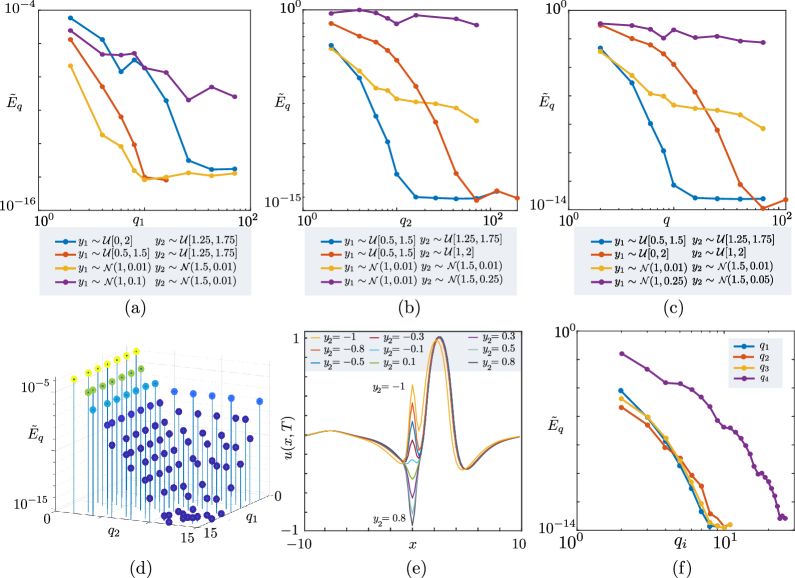
Figure 4: Convergence of stochastic collocation error $\tilde{E}_{q}$ Eq. 52, for the NRNF problem in Eqs. 50 to 51 with $2$- and $4$-dimensional random noise. (a) We fix the number of collocation points in the $y_{2}$-direction and refine the tensor grid along $y_{1}$-direction. We set $q^{*}_{2}=10$ for the normal distribution and $q^{*}_{2}=64$ for the uniform ones. The number $q^{*}_{1}$ is taken as large as possible to test convergence, but differs for each curve. In (b), we fix $q^{*}_{1}=16$ in both normal and uniform settings, and increase $q_{2}$. In (c), we increase $q_{1}=q_{2}=q$ simultaneously, and we plot $q$. In (a–c) we note that the error in $y_{2}$ dominates over the one in $y_{1}$, and slower convergence is observed when the variance increases. In (d), the noise in the external input and the initial condition depends on $y_{1}\sim\mathcal{U}[1.25,1.75]$ and $y_{2}\sim\mathcal{U}[0.5,1.5]$ and we show an experiment in which $q^{*}=(15,15)$ is kept fixed for all simulations. $(e)$ We show nine solution profiles at final time $T$ of the NRNF, for $y_{1}=1$ and ten different values of the parameter $y_{2}\in[-1,0.8]$, giving evidence of a bifurcation in this parameter range, and explaining the lower convergence rates seen in (a–c) for normally-distributed parameters (see main text). In (f) we refine one grid direction at a time for the NRNF with 4 parameters, as given in Section 7.3. Other parameter values are: $\sigma_{\omega}=1$, $F_{0}=1$, $\mu=10$, $h=0.3$, $\omega_{g}=1$ and $\sigma_{g}=0.4$, $n^{*}=40$, $T=1$.

7.3 Problem 3: nonlinear case, uniformly distributed random parameters in $\mathbb{R}^{4}$

In a final test we amend Problem 2 and make the variables $A_{0}$ and $F_{0}$ uniformly distributed, so that all input data is random, with $y\in\mathbb{R}^{4}$. Figure 4(f) displays $\tilde{E}_{q}$ as we refine points one direction at a time, and confirms that similar convergence rates to the case $y\in\mathbb{R}^{2}$ can be attained in this case.

8 Conclusions

In this paper we have introduced a scheme for forward UQ in neural field models, using stochastic collocation. The method adapts stochastic collocation from PDE literature to integro-differential equations arising in mathematical neuroscience, and it combines with generic spatial discretisations for the problem. The method presented here can be readily implemented to perform UQ, upon coding the spatially-projected forward simulation problem within existing UQ software such as Sparse Grids Matlab Kit [42] and UQLab [35].

It seems possible to study variations of stochastic collocation which, in the PDE literature, overcome some of the limitations of the method, and are suitable for a large number of parameters, in particular sparse grid, sparse Galerkin, and anisotripic methods [40, 39, 28, 29, 24, 1]. Further, we expect that a similar approach to the one taken here, which splits the spatial and stochastic error for the problem, will help us analysing Monte Carlo Finite Element schemes and its variants (in particular we should be able to adapt directly the methods in [34, Chapter 9]). An immediate application of the theory presented in this paper is the use of stochastic collocation for Bayesian inverse problems in neural fields, which can follow its PDE analogues [37] and is promising for low-dimensional parametrised problems.

Appendix A Perturbative result on semigroup operator

The proof of $C^{0}_{\sigma}$-regularity for the solution uses the following perturbative result on operator semigroups

Lemma A.1 (Perturbation of semigroup operators).

Let $A,B\in BL(\mathbb{X})$, where $\mathbb{X}$ is a Banach space. The uniformly continuous semigroups $(e^{tA})_{t\geq 0}$, $(e^{tB})_{t\geq 0}$, generated on $\mathbb{X}$ by $A$ and $B$, respectively, satisfy

$$\|e^{tA}-e^{tB}\|\leq t\|A-B\|e^{t\|A-B\|}e^{t\min(\|A\|,\|B\|)},\qquad t\in\mathbb{R}_{\geq 0}.$$

Proof A.2.

By [21, Chapter III, Section 1, Corollary 1.7] it holds

(53) $$(e^{tB}-e^{tA})v=\int_{0}^{t}e^{(t-s)A}(B-A)e^{sB}v\,ds,\qquad v\in\mathbb{X},\qquad t\in\mathbb{R}_{\geq 0}.$$

Taking norms, and recalling $\|e^{tA}\|\leq e^{t\|A\|}$ for any $A\in BL(\mathbb{X})$ and $t\in\mathbb{R}_{\geq 0}$ we get

$$\|(e^{tB}-e^{tA})v\| \leq\|B-A\|\|v\|\int_{0}^{t}e^{t\|A\|}e^{s(\|B\|-\|A\|)}\,ds$$

$$\leq\|B-A\|\|v\|e^{t\|A\|}\int_{0}^{t}e^{s\|B-A\|}\,ds$$

$$<t\|A-B\|e^{t\|A-B\|}e^{t\|A\|}\|v\|,$$

hence

$$\|e^{tA}-e^{tB}\|\leq t\|A-B\|e^{t\|A-B\|}e^{t\|A\|},\qquad t\in\mathbb{R}_{\geq 0}.$$

Swapping $A$ and $B$ in Eq. 53 we obtain

$$\|e^{tA}-e^{tB}\|\leq t\|A-B\|e^{t\|A-B\|}e^{t\|B\|},\qquad t\in\mathbb{R}_{\geq 0},$$

and combining the last two bounds we prove the statement.

Appendix B Further proofs

References

- [1] B. Adcock, S. Brugiapaglia, and C. G. Webster, Sparse Polynomial Approximation of High-Dimensional Functions, Society for Industrial and Applied Mathematics, Philadelphia, PA, Jan. 2022, https://doi.org/10.1137/1.9781611976885.
- [2] S.-i. Amari, Dynamics of pattern formation in lateral-inhibition type neural fields, Biological Cybernetics, 27 (1977), pp. 77–87.
- [3] K. E. Atkinson, A Survey of Numerical Methods for Solving Nonlinear Integral Equations, Journal of Integral Equations and Applications, 4 (1992), pp. 15–46.
- [4] K. E. Atkinson, The Numerical Solution of Integral Equations of the Second Kind, Cambridge Monographs on Applied and Computational Mathematics, Cambridge University Press, 1997, https://doi.org/10.1017/CBO9780511626340.
- [5] K. E. Atkinson and W. Han, Theoretical numerical analysis, vol. 39, Springer, 2005.
- [6] D. Avitabile, Projection Methods for Neural Field Equations, SIAM Journal on Numerical Analysis, 61 (2023), pp. 562–591, https://doi.org/10.1137/21M1463768.
- [7] D. Avitabile, Projection methods for neural field equations. https://www.codeocean.com/, 11 2024, https://doi.org/10.24433/CO.3131389.v1.
- [8] D. Avitabile, Tutorials on Numerical and Analytical Methods for Spatially-Extended Neurobiological Networks, 04 2024, https://doi.org/10.5281/zenodo.11124322, https://github.com/danieleavitabile/numerical-analysis-mathematical-neuroscience.
- [9] D. Avitabile, F. Cavallini, S. Dubinkina, and G. J. Lord, Neural field equations with random data, 2025, https://arxiv.org/abs/2505.16343, https://arxiv.org/abs/2505.16343.
- [10] D. Avitabile, J. L. Davis, and K. Wedgwood, Bump Attractors and Waves in Networks of Leaky Integrate-and-Fire Neurons, SIAM Review, 65 (2023), pp. 147–182, https://doi.org/10.1137/20M1367246.
- [11] D. Avitabile and H. Schmidt, Snakes and ladders in an inhomogeneous neural field model, Physica D: Nonlinear Phenomena, 294 (2015), pp. 24–36, https://doi.org/10.1016/j.physd.2014.11.007.
- [12] I. Babuška, F. Nobile, and R. Tempone, A Stochastic Collocation Method for Elliptic Partial Differential Equations with Random Input Data, SIAM Journal on Numerical Analysis, 45 (2007), pp. 1005–1034, https://doi.org/10.1137/050645142, http://epubs.siam.org/doi/10.1137/050645142 (accessed 2022-03-20).
- [13] I. Babuska, R. Tempone, and G. E. Zouraris, Galerkin Finite Element Approximations of Stochastic Elliptic Partial Differential Equations, SIAM Journal on Numerical Analysis, 42 (2004), pp. 800–825, https://doi.org/10.1137/S0036142902418680.
- [14] P. C. Bressloff, Waves in Neural Media, Springer New York, Springer New York, 2014, https://doi.org/10.1007/978-1-4614-8866-8.
- [15] P. C. Bressloff and J. D. Cowan, A spherical model for orientation and spatial–frequency tuning in a cortical hypercolumn, Philosophical Transactions of the Royal Society of London. Series B: Biological Sciences, 358 (2003), pp. 1643–1667.
- [16] B. Buffoni and J. Toland, Analytic Theory of Global Bifurcation: An Introduction, Princeton University Press, Princeton, N.J, 1st edition ed., Feb. 2003.
- [17] S. Coombes, P. beim Graben, R. Potthast, and J. Wright, Neural fields: theory and applications, Springer, 2014.
- [18] M. Corti, F. Bonizzoni, P. F. Antonietti, and A. M. Quarteroni, Uncertainty quantification for Fisher-Kolmogorov equation on graphs with application to patient-specific Alzheimer’s disease, ESAIM: Mathematical Modelling and Numerical Analysis, 58 (2024), pp. 2135–2154, https://doi.org/10.1051/m2an/2023095.
- [19] J. L. Daleckii and M. G. Kre_n, Stability of Solutions of Differential Equations in Banach Space, no. 43, American Mathematical Soc., 2002.
- [20] A. Defant and K. Floret, Tensor Norms and Operator Ideals, North Holland, Amsterdam ; New York, 1st edition ed., Nov. 1992.
- [21] K.-J. Engel and R. Nagel, A short course on operator semigroups, Springer Science & Business Media, 2006.
- [22] K.-J. Engel, R. Nagel, and S. Brendle, One-Parameter Semigroups for Linear Evolution Equations, vol. 194, Springer, 2000.
- [23] B. Ermentrout, Neural networks as spatio-temporal pattern-forming systems, Reports on Progress in Physics, 61 (1998), pp. 353 – 430, https://doi.org/10.1088/0034-4885/61/4/002.
- [24] O. G. Ernst, B. Sprungk, and L. Tamellini, Convergence of Sparse Collocation for Functions of Countably Many Gaussian Random Variables (with Application to Elliptic PDEs), SIAM Journal on Numerical Analysis, 56 (2018), pp. 877–905, https://doi.org/10.1137/17M1123079.
- [25] O. Faugeras, F. Grimbert, and J.-J. Slotine, Absolute stability and complete synchronization in a class of neural fields models, SIAM Journal on applied mathematics, 69 (2008), pp. 205–250.
- [26] P. Frauenfelder, C. Schwab, and R. A. Todor, Finite elements for elliptic problems with stochastic coefficients, Computer Methods in Applied Mechanics and Engineering, 194 (2005), pp. 205–228, https://doi.org/10.1016/j.cma.2004.04.008.
- [27] R. Ghanem and P. D. Spanos, Stochastic Finite Elements: A Spectral Approach, Dover Publ, Mineola, NY, rev. ed ed., 2003.
- [28] M. Hansen and C. Schwab, Sparse Adaptive Approximation of High Dimensional Parametric Initial Value Problems, Vietnam Journal of Mathematics, 41 (2013), pp. 181–215, https://doi.org/10.1007/s10013-013-0011-9.
- [29] V. H. Hoang and C. Schwab, Sparse Tensor Galerkin Discretization of Parametric and Random Parabolic PDEs—Analytic Regularity and Generalized Polynomial Chaos Approximation, SIAM Journal on Mathematical Analysis, 45 (2013), pp. 3050–3083, https://doi.org/10.1137/100793682.
- [30] X. Huang, W. Xu, J. Liang, K. Takagaki, X. Gao, and J.-y. Wu, Spiral wave dynamics in neocortex, Neuron, 68 (2010), pp. 978–990.
- [31] L. J. Roman, M. Sarkis, and ,Worcester Polytechnic Institute, Department of Mathematical Sciences, 100 Institute Rd, Worcester, MA 01609-2280, Stochastic Galerkin method for elliptic spdes: A white noiseapproach, Discrete & Continuous Dynamical Systems - B, 6 (2006), pp. 941–955, https://doi.org/10.3934/dcdsb.2006.6.941.
- [32] S. S. Kim, H. Rouault, S. Druckmann, and V. Jayaraman, Ring attractor dynamics in the Drosophila central brain, Science, 356 (2017), pp. 849–853, https://doi.org/10.1126/science.aal4835.
- [33] S.-H. Lee, R. Blake, and D. J. Heeger, Traveling waves of activity in primary visual cortex during binocular rivalry, Nature neuroscience, 8 (2005), pp. 22–23.
- [34] G. J. Lord, C. E. Powell, and T. Shardlow, An introduction to computational stochastic PDEs, Cambridge University Press, Cambridge, Jan. 2014.
- [35] S. Marelli and B. Sudret, UQLab: A Framework for Uncertainty Quantification in Matlab, in Vulnerability, Uncertainty, and Risk, Liverpool, UK, June 2014, American Society of Civil Engineers, pp. 2554–2563, https://doi.org/10.1061/9780784413609.257.
- [36] R. Martin, D. J. Chappell, N. Chuzhanova, and J. J. Crofts, A numerical simulation of neural fields on curved geometries, Journal of computational neuroscience, 45 (2018), pp. 133–145.
- [37] Y. Marzouk and D. Xiu, A Stochastic Collocation Approach to Bayesian Inference in Inverse Problems, Communications in Computational Physics, 6 (2009), pp. 826–847, https://doi.org/10.4208/cicp.2009.v6.p826.
- [38] F. Nobile and R. Tempone, Analysis and implementation issues for the numerical approximation of parabolic equations with random coefficients, International Journal for Numerical Methods in Engineering, 80 (2009), pp. 979–1006, https://doi.org/10.1002/nme.2656.
- [39] F. Nobile, R. Tempone, and C. G. Webster, An Anisotropic Sparse Grid Stochastic Collocation Method for Partial Differential Equations with Random Input Data, SIAM Journal on Numerical Analysis, 46 (2008), pp. 2411–2442, https://doi.org/10.1137/070680540.
- [40] F. Nobile, R. Tempone, and C. G. Webster, A Sparse Grid Stochastic Collocation Method for Partial Differential Equations with Random Input Data, SIAM Journal on Numerical Analysis, 46 (2008), pp. 2309–2345, https://doi.org/10.1137/060663660.
- [41] J. C. Pang, K. M. Aquino, M. Oldehinkel, P. A. Robinson, B. D. Fulcher, M. Breakspear, and A. Fornito, Geometric constraints on human brain function, Nature, 618 (2023), pp. 566–574, https://doi.org/10.1038/s41586-023-06098-1.
- [42] C. Piazzola and L. Tamellini, Algorithm 1040: The Sparse Grids Matlab Kit - a Matlab implementation of sparse grids for high-dimensional function approximation and uncertainty quantification, ACM Transactions on Mathematical Software, 50 (2024), https://doi.org/10.1145/3630023.
- [43] R. Potthast and P. beim Graben, Existence and properties of solutions for neural field equations, Mathematical Methods in the Applied Sciences, 33 (2010), pp. 935–949.
- [44] P. A. Robinson, C. J. Rennie, and J. J. Wright, Propagation and stability of waves of electrical activity in the cerebral cortex, Physical Review E, 56 (1997), p. 826.
- [45] S. B. Shaw, Z. P. Kilpatrick, and D. Avitabile, Radial basis function techniques for neural field models on surfaces, 2025, https://arxiv.org/abs/2504.13379, https://arxiv.org/abs/2504.13379.
- [46] R. C. Smith, Uncertainty Quantification: Theory, Implementation, and Applications, no. 12 in Computational Science & Engineering, siam, Society for Industrial and Applied Mathematics, Philadelphia, 2014.
- [47] G. Van Damme, Legendre Laguerre and Hermite Gauss Quadrature, 05 2025, https://www.mathworks.com/matlabcentral/fileexchange/26737-legendre-laguerre-and-hermite-gauss-quadrature (accessed 2025/05/18).
- [48] J. van Neerven, Functional Analysis, Cambridge University Press, 1 ed., July 2022, https://doi.org/10.1017/9781009232487, https://www.cambridge.org/core/product/identifier/9781009232487/type/book (accessed 2022-11-26).
- [49] S. Visser, R. Nicks, O. Faugeras, and S. Coombes, Standing and travelling waves in a spherical brain model: The Nunez model revisited., Physica D, 349 (2017), pp. 27 – 45, https://doi.org/10.1016/j.physd.2017.02.017.
- [50] G. von Winckel, Legendre-Gauss Quadrature Weights and Nodes, 05 2025, https://www.mathworks.com/matlabcentral/fileexchange/4540-legendre-gauss-quadrature-weights-and-nodes (accessed 2025/05/18).
- [51] H. R. Wilson and J. D. Cowan, A mathematical theory of the functional dynamics of cortical and thalamic nervous tissue, Kybernetik, 13 (1973), pp. 55–80.
- [52] D. Xiu and G. Em Karniadakis, Modeling uncertainty in steady state diffusion problems via generalized polynomial chaos, Computer Methods in Applied Mechanics and Engineering, 191 (2002), pp. 4927–4948, https://doi.org/10.1016/S0045-7825(02)00421-8.
- [53] D. Xiu and J. S. Hesthaven, High-Order Collocation Methods for Differential Equations with Random Inputs, SIAM Journal on Scientific Computing, 27 (2005), pp. 1118–1139, https://doi.org/10.1137/040615201.
- [54] E. Zeidler, Nonlinear Functional Analysis and Its Applications I: Fixed Point Theorems, Springer, Springer, 1985.
- [55] G. Zhang and M. Gunzburger, Error Analysis of a Stochastic Collocation Method for Parabolic Partial Differential Equations with Random Input Data, SIAM Journal on Numerical Analysis, 50 (2012), pp. 1922–1940, https://doi.org/10.1137/11084306x.