TriggerCalib: a turnkey package for estimating LHCb trigger efficiencies

Abstract

Data-driven estimations of trigger efficiencies are essential to LHCb physics analyses. A software package, TriggerCalib, has been developed to provide a centralised framework of trigger efficiency calculations. In this paper, a data-driven method of estimating trigger efficiencies is presented, within the context of the TriggerCalib package, and its functionalities validated on candidate ${{{B}^{+}}}\!\rightarrow{{J\mskip-3.0mu/\mskip-2.0mu\psi}}{{K}^{+}}$ decays in LHCb simulated data. A detailed overview of the trigger efficiency calculations is given, discussing different background mitigation methods and the computation of statistical and systematic uncertainties.

1 Introduction

This paper presents the TriggerCalib, standing for Trigger Calibration, software package, which is a set of data analysis tools designed to help analysts to determine efficiencies of trigger selections in the LHCb dataflow.

The LHCb experiment [1, 2] is a forward single-arm spectrometer at the LHC, optimised for the study of heavy-flavour hadrons and primarily instrumented in the pseudorapidity range $2<\eta<5$. It collected proton-proton (${p}\!{p}$) collision data between 2011 and 2018 during the LHC Run 1-2, reaching an integrated luminosity of 9 $\text{\,fb}^{-1}$. Subsequently, it underwent a major upgrade [3] of the detectors and data acquisition system with the aim of collecting data with a five times greater instantaneous luminosity than the original experiment, reaching ${\mathcal{L}=2\times 10^{33}\text{\,cm}^{-2}\text{\,s}^{-1}}$ during the LHC Run 3 from 2022 to 2026.

The upgraded LHCb detector must cope with the 30 MHz rate of ${p}\!{p}$ bunch collision events provided by the LHC. Contrary to Run 1, where a hardware trigger was employed to perform the initial reduction in data rate, a software-only trigger system reduces the large input data rate of 4 TB/s to $\mathcal{O}(10\,\text{GB/s})$ using selections, referred to as “lines", primarily based on reconstructed objects and decay topologies. This is implemented as a two-stage High Level Trigger (HLT) processing pipeline deployed in a heterogeneous custom data centre [4]. The first stage (HLT1) is based on GPU processors and performs a partial event reconstruction to reduce the data rate by a factor of 40, reaching an output rate of around 100 GB/s. The data are then buffered while the detector alignment and calibration procedures are performed. This approach allows for full offline-quality event reconstruction in the second trigger stage (HLT2), which is executed entirely on CPU processors. Finally, the data are processed through the offline analysis framework, providing the input for physics analyses [5, 6].

The software used in both trigger stages includes a set of algorithms that process the information from the LHCb subdetectors to reconstruct and select processes of interest to the LHCb physics programme. The electronic responses of the subdetectors are used for four main reconstruction tasks:

• tracking, reconstructing trajectories of particles from hits in the LHCb subdetectors;

• vertexing, searching for the origin locations of ${p}\!{p}$ collisions or of decaying particles;

• particle identification, distinguishing charged final state particles’ nature;

• neutral particle reconstruction, reconstructing neutral particles, such as photons and ${\pi}^{0}$ mesons, from calorimeter information.

Simulation is required to model the effects of the detector acceptance and the imposed selection requirements. In the simulation, $pp$ collisions are generated using Pythia [7, 8] with a specific LHCb configuration [9]. Decays of unstable particles are described by EvtGen [10], in which final-state radiation is generated using Photos [11]. The interaction of the generated particles with the detector, and its response, are implemented using the Geant4 toolkit [12, 13] as described in Ref. [14].

The simulation of such a complex system of subdetectors and their response to particle physics phenomena is non-trivial and requires accurate modelling of particle kinematics, the occupancy of the subdetectors and the experimental conditions. Inaccuracies in the simulation of the detector and/or physics processes can lead to biases of the trigger response in simulation and, therefore, of the trigger efficiency. These considerations motivated analysts to implement data-driven techniques to measure the factors contributing to the detection efficiency, including that of the trigger.

This paper provides first in Section 2 an overview of the so-called “$\mathrm{TISTOS}$” method of determining trigger efficiencies. This method has already been used in many LHCb physics analyses. The TriggerCalib package provides a central implementation of the $\mathrm{TISTOS}$ method with generalised tools to evaluate efficiencies and correct the trigger response in simulated samples. These tools are introduced in Section 3, presenting their validation with different background mitigation methods as a function of different kinematic variables. Finally, a discussion on the computation of statistical and systematic uncertainties is reported in Section 4.

The decay ${{{B}^{+}}}\!\rightarrow{{J\mskip-3.0mu/\mskip-2.0mu\psi}}\left({\mu^{+}\mu^{-}}\right){{K}^{+}}$ is widely used as a control channel in LHCb analyses, and is characterized by high statistics and purity. In Run 3, these decays are selected at a rate of $\mathcal{O}\left(10\text{\,Hz}\right)$. The studies presented in this paper were performed on a sample of simulated ${{{B}^{+}}}\!\rightarrow{{J\mskip-3.0mu/\mskip-2.0mu\psi}}\left({\mu^{+}\mu^{-}}\right){{K}^{+}}$ decays, subject to selection by a dedicated ${{{B}^{+}}}\!\rightarrow{{J\mskip-3.0mu/\mskip-2.0mu\psi}}\left({\mu^{+}\mu^{-}}\right){{K}^{+}}$ HLT2 line and further selection cuts on kinematic, topological and particle-identification properties applied offline. A toy combinatorial background is added to this sample to demonstrate the background mitigation methods implemented in TriggerCalib. The generation of this background is described in Appendix A. Generally, the $\mathrm{TISTOS}$ method, and by extension the set of tools available in TriggerCalib, are applicable to any decay channel and dataset.

2 The TISTOS method for trigger efficiencies

Evaluating trigger efficiencies in data is not a trivial task. Whilst the recorded dataset contains only triggered events, there is sufficient redundancy between different trigger selections and signals to allow the trigger efficiencies to be estimated from these data, Since this redundancy is insufficient to construct an efficiency as the simple fraction of events passing a given trigger selection, the LHCb Collaboration developed a fully data-driven approach to evaluate such efficiencies. This method, referred to as the $\mathrm{TISTOS}$ method, was first introduced in Ref. [15], is described in Refs. [16, 17] and has been used extensively in the LHCb physics program. The method is defined in the context of $b$-decays, though in some cases can be extended to other processes studied at LHCb.

A subsample of events selected by a certain trigger, tag events, must be defined such that some of these, the probe events, are also selected by the trigger of interest. The efficiency of the trigger of interest for tag events is assumed to be representative of all events in the dataset. However, the tag and probe may be correlated and this correlation must be taken into account when applying the $\mathrm{TISTOS}$ method.

2.1 Trigger categories

Three trigger categories are defined in order to construct data-driven efficiency estimators. These categories are assigned after selecting a signal candidate within each event in the data sample. A signal candidate in the recorded dataset is characterised by the momenta and other high-level information describing the final-state particles. The detector hits associated with the final-state particles are also retained.

For each trigger selection, the candidate can be:

• Triggered on signal (TOS): the signal candidate is sufficient for the trigger decision, regardless of the rest of the event;

• Triggered independently of signal (TIS): another reconstructed object in the event is sufficient for the trigger decision, regardless of the signal candidate.

• Triggered on signal and independently of signal (TISTOS): the intersection of the two cases above.

Additionally, the case where the signal or rest of event alone are insufficient for a trigger decision but their combination is sufficient is dubbed triggered on both (TOB). However, as few events are TOB, estimated at 0.5% for $b$-decays [16], this is not discussed in this paper.

The $\mathrm{TIS}$ and $\mathrm{TOS}$ categories are associated to each signal candidate by comparing the detector hits of the signal candidate with the detector hits of all selected candidates in the given event. A signal candidate is categorised $\mathrm{TOS}$ if at least $70\%$ of the hits across all selected candidates in the event are hits involved in reconstructing the signal candidate. Likewise, if any candidate in the event besides the signal candidate shares fewer than $1\%$ of hits with the signal candidate, then the signal candidate is categorised as $\mathrm{TIS}$. For a composite signal candidate, the associated hits are taken to be the combined hits of all of the corresponding final state particles.

2.2 The TISTOS method

The trigger efficiency for a given decision can be expressed in terms of the categories defined in the previous section:

$$\varepsilon_{\mathrm{Trig.}}=\frac{N_{\mathrm{Trig.}}}{N_{\mathrm{Tot.}}}=\frac{N_{\mathrm{Trig.}}}{N_{\mathrm{TIS}}}\times\frac{N_{\mathrm{\mathrm{TIS}}}}{N_{\mathrm{Tot.}}}=\frac{N_{\mathrm{Trig.}}}{N_{\mathrm{TIS}}}\times\varepsilon_{\mathrm{TIS}},$$ (2.1)

where $N_{\mathrm{Trig.}}$ is the number of events passing the given selection, $N_{\mathrm{Tot.}}$ the total number of events (triggered and not-triggered) and $N_{\mathrm{\mathrm{TIS}}}$ the number of $\mathrm{TIS}$ events. The TIS efficiency $\varepsilon_{\mathrm{TIS}}$ is not directly measurable in data. $\varepsilon_{\mathrm{TIS}}$ is equal, within small or accountable correlations, to the efficiency evaluated within a tag $\mathrm{TOS}$ subsample as:

$$\varepsilon_{\mathrm{TIS}}\equiv\varepsilon_{\mathrm{TIS}\mid\mathrm{TOS}}=\frac{N_{\mathrm{TISTOS}}}{N_{\mathrm{TOS}}},$$ (2.2)

wherein $N_{\mathrm{\mathrm{TISTOS}}}$ is the number of events which are both $\mathrm{TIS}$ and $\mathrm{TOS}$, and $N_{\mathrm{\mathrm{TOS}}}$ is the number of $\mathrm{TOS}$ events. From this definition, Equation 2.1 can be written in the form:

$$\varepsilon_{\mathrm{Trig.}}=\frac{N_{\mathrm{Trig.}}}{N_{\mathrm{TIS}}}\times\frac{N_{\mathrm{TISTOS}}}{N_{\mathrm{TOS}}},$$ (2.3)

where all elements can be directly computed in data.

Analogously to Equation 2.2, one can define the $\mathrm{TOS}$ efficiency on a tag subsample of $\mathrm{TIS}$ events as:

$$\varepsilon_{\mathrm{TOS}}\equiv\varepsilon_{\mathrm{TOS}\mid\mathrm{TIS}}=\frac{N_{\mathrm{TISTOS}}}{N_{\mathrm{TIS}}}.$$ (2.4)

Correlations between the tag and probe samples in each efficiency may lead to biases in the efficiency evaluation.

In particular, heavy-flavour hadrons are usually produced in pairs in $p$ ​$p$ collisions, following the production of heavy-flavour quark and antiquark pairs. Therefore, the kinematics of the signal candidate may be correlated to other candidates considered independent of signal. As trigger selections rely heavily upon requirements on the momentum and impact parameter of the decay products, the assumption of tag and probe independence can create a bias in the evaluation of trigger efficiencies when integrating over all phase space.

2.3 Kinematic dependence

Kinematic correlations between the $\mathrm{TIS}$ and $\mathrm{TOS}$ subsamples might bias the evaluation of the trigger efficiencies with the $\mathrm{TISTOS}$ method. As shown in Figure 1, the transverse momentum ($p_{\mathrm{T}}$) of ${{B}^{+}}$ mesons decaying as ${{{B}^{+}}}\!\rightarrow{{J\mskip-3.0mu/\mskip-2.0mu\psi}}\left({\mu^{+}\mu^{-}}\right){{K}^{+}}$ is harder when selected as $\mathrm{TIS}$ events, compared to those selected without any specific trigger filtering. This would result in over-estimated trigger efficiencies when computed on $\mathrm{TIS}$ events with the $\mathrm{TISTOS}$ data-driven method. It is therefore necessary to evaluate the efficiency in phase-space intervals.

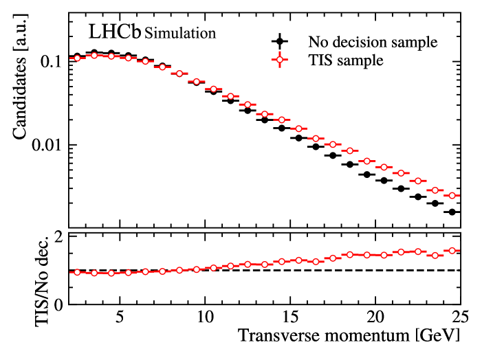
Figure 1: Transverse momentum ($p_{\mathrm{T}}$) distributions of simulated ${{{B}^{+}}}\!\rightarrow{{J\mskip-3.0mu/\mskip-2.0mu\psi}}\left({\mu^{+}\mu^{-}}\right){{K}^{+}}$ decays selected by $\mathrm{TIS}$ decisions and without any decisions required.

One can express Equation 2.3 in terms of a sum over event kinematic regions $i$:

$$\varepsilon_{\mathrm{Trig.}}=\frac{N_{\mathrm{Trig.}}}{\sum\limits_{i}N_{\mathrm{Tot.}}^{i}}=\frac{N_{\mathrm{Trig.}}}{\sum\limits_{i}\frac{N_{\mathrm{TIS}}^{i}}{\varepsilon_{\mathrm{TIS}}^{i}}}=\frac{N_{\mathrm{Trig.}}}{\sum\limits_{i}\frac{N_{\mathrm{TIS}}^{i}N_{\mathrm{TOS}}^{i}}{N_{\mathrm{TISTOS}}^{i}}}.$$ (2.5)

Equation 2.5 can also be used to study dependences from multiple degrees of freedom, e.g., by varying the kinematic binning of the sample. As reported in Ref. [16], by increasing the number of regions in each dimension, the efficiency evaluated with the $\mathrm{TISTOS}$ method approaches the fraction of events passing the selection as computed from a truth-level simulated sample.

In fact, by choosing small enough kinematic regions, the trigger efficiencies evaluated with the $\mathrm{TISTOS}$ method become largely unbiased by the correlations between the $\mathrm{TIS}$ and $\mathrm{TOS}$ events, as demonstrated by these studies.

Different decay kinematic variables should be tested when evaluating trigger efficiencies, such as the momentum, transverse momentum, pseudorapidity, lifetime or occupancy regions of the events. The TriggerCalib package presented in the next section provides analysts the flexibility of choosing between any variable and phase-space division schemes.

3 The TriggerCalib software package

The TriggerCalib software package implements the $\mathrm{TISTOS}$ method as set of Python-based tools for use in analyses of LHCb data. This central implementation allays the need for trigger-specific expertise to implement the $\mathrm{TISTOS}$ calculations accurately in analyses.

Two different aspects are proposed and implemented in the software:

• data-driven efficiency evaluation: computation of trigger efficiencies directly on data with the $\mathrm{TISTOS}$ method, namely on channels with high statistics and well-understood backgrounds;

• simulation corrections: evaluation of per-event correction weights which can be applied to simulated samples to correct the trigger response, e.g., in channels where insufficient statistics allow for direct evaluation of the trigger efficiencies, corrections can be computed in a higher statistics reference channel and applied to simulation representative of the target channel.

The choice of approach depends on the type of analysis performed, the signal channel studied and the trigger selection(s) of interest. For sufficiently large datasets, the direct evaluation of efficiencies on data should be chosen, whilst the data-simulation correction approach should be used when studying rare processes with limited signal yields. Correction weights can be evaluated on an abundant control sample with similar kinematics and topology to the signal channel and then applied to simulated samples of the signal decay. With this approach, the trigger efficiencies can then be computed directly on the re-weighted simulated sample. The framework allows the use of both approaches giving the flexibility to exploit the $\mathrm{TISTOS}$ method with any set of phase-space regions. In data, background mitigation methods must be applied to retrieve the $\mathrm{TISTOS}$ yields. Three such methods are implemented in the package and discussed in the next section.

The following studies use a simulated sample of ${{{B}^{+}}}\!\rightarrow{{J\mskip-3.0mu/\mskip-2.0mu\psi}}\left({\mu^{+}\mu^{-}}\right){{K}^{+}}$ decays, reflecting the data-taking conditions of 2024. This sample is supplemented with an artificial combinatorial background component, described in Appendix A.

These studies focuses on the evaluation of the efficiency of two important trigger selections at the first-level trigger (HLT1) at LHCb:

• HLT1TrackMVA, which selects candidates with a significantly displaced and high-momentum charged particle;

• HLT1TwoTrackMVA, which selects candidates with a good quality and displaced two-particle vertex at high combined momenta.

These two trigger decisions are used by many LHCb analyses and therefore constitute a representative benchmark for our studies. In the next sections, when demonstrating the methods for a given trigger selection, the combination of the HLT1TrackMVA and HLT1TwoTrackMVA decisions on the $B^{+}$ candidate is assumed for the triggered, $\mathrm{TOS}$ and $\mathrm{TIS}$ categories.

3.1 Background subtraction approaches

To obtain reliable trigger efficiencies with respect to a given channel, the yields used by the $\mathrm{TISTOS}$ method must contain a negligible amount of background. Background contributions are mitigated by either subtracting the corresponding amount of background or by direct modelling of the background component(s). Three methods of background mitigation are implemented in TriggerCalib:

• Sideband subtraction: signal and sideband windows are defined in the invariant mass distribution of the signal particle studied. In each phase-space region, the density of events in the sideband window is taken as an estimate of the density of background events within the signal region and subtracted from the signal region accordingly;

• Fit-and-count: a statistical model containing components describing signal and background is fit to the invariant mass distribution of the channel studied in each phase-space region. The yield of the signal component in the model is used to evaluate the efficiency;

• sPlot: a statistical model is fit globally (i.e., integrated over the other phase-space dimensions) to the invariant mass of the signal particle studied. Per-event sWeights are calculated for each component of the fit according to the sPlot method [18]. Signal sWeights are applied to the distribution(s) of interest, which can then be binned in phase-space regions to evaluate the $\mathrm{TISTOS}$ yields.

The sideband subtraction method provides a simple and robust approach across the phase space, even when dealing with kinematic regions with fewer events. However, it is valid only when a simple description of the background component is possible. Contrarily, when studying events from datasets with larger and more complex backgrounds, the fit-and-count and sPlot methods become crucial in order to calculate reliable trigger efficiencies.

The three methods are tested with ${{{B}^{+}}}\!\rightarrow{{J\mskip-3.0mu/\mskip-2.0mu\psi}}\left({\mu^{+}\mu^{-}}\right){{K}^{+}}$ candidates to assess their validity and performance as function of the phase space. The discriminating variable used corresponds to the invariant mass of ${{B}^{+}}$ meson candidates, computed from the combination of the ${J\mskip-3.0mu/\mskip-2.0mu\psi}$ and ${K}^{+}$.

3.1.1 Sideband subtraction

The sideband subtraction method can be used under the assumption that the only background component(s) has an approximately linear dependence on the discriminating variable.

Within a total invariant mass window ($\Delta_{\mathrm{total}}$) in the sample studied, a signal region ($\Delta_{\mathrm{signal}}$) can be defined around the signal mass peak. Similarly, sideband windows ($\Delta_{\mathrm{sideband}}^{i}$) can be defined which contain only the underlying background. The signal yield can then be defined as function of the yield in the total mass window ($N_{\mathrm{total}}$) and a background density ($\rho$) as:

$$N_{\mathrm{signal}}=N_{\mathrm{total}}-\Delta_{\mathrm{signal}}\cdot\rho\quad\quad\mathrm{where}\quad\quad\rho=\frac{\sum\limits_{i}N^{i}_{\mathrm{sideband}}}{\sum\limits_{i}\Delta^{i}_{\mathrm{sideband}}},$$ (3.1)

with $N^{i}_{\mathrm{sideband}}$ the yields in the sideband regions. This holds for all approximately constant backgrounds, and more generally holds so long as the sideband windows are chosen carefully to reflect the shape of the background. The method can then be applied in regions of the phase-space to evaluate the $\mathrm{TIS}$, $\mathrm{TOS}$ and $\mathrm{TISTOS}$ filtered yields and compute the trigger efficiency with Equation 2.5.

In the ${{{B}^{+}}}\!\rightarrow{{J\mskip-3.0mu/\mskip-2.0mu\psi}}\left({\mu^{+}\mu^{-}}\right){{K}^{+}}$ sample analysed in this study, the invariant mass window $m\left({{J\mskip-3.0mu/\mskip-2.0mu\psi}}{{K}^{+}}\right)\in\left[5200,375\right]\text{\,Me\kern-1.00006ptV\!/}c^{2}$ is considered. The signal region is defined around the mass of the ${{B}^{+}}$ [19] to be $m\left({{J\mskip-3.0mu/\mskip-2.0mu\psi}}{{K}^{+}}\right)\in\left[5255,5310\right]\text{\,Me\kern-1.00006ptV\!/}c^{2}$. The sidebands are defined here to extend from the limits of the total window up to 10 MeV from each signal window limit. The background is mainly composed of random combinations of tracks which are reconstructed and selected as candidates, so-called combinatorial background. The signal and sideband windows are shown in Figure 2, along with the sideband-subtracted distribution of candidates.

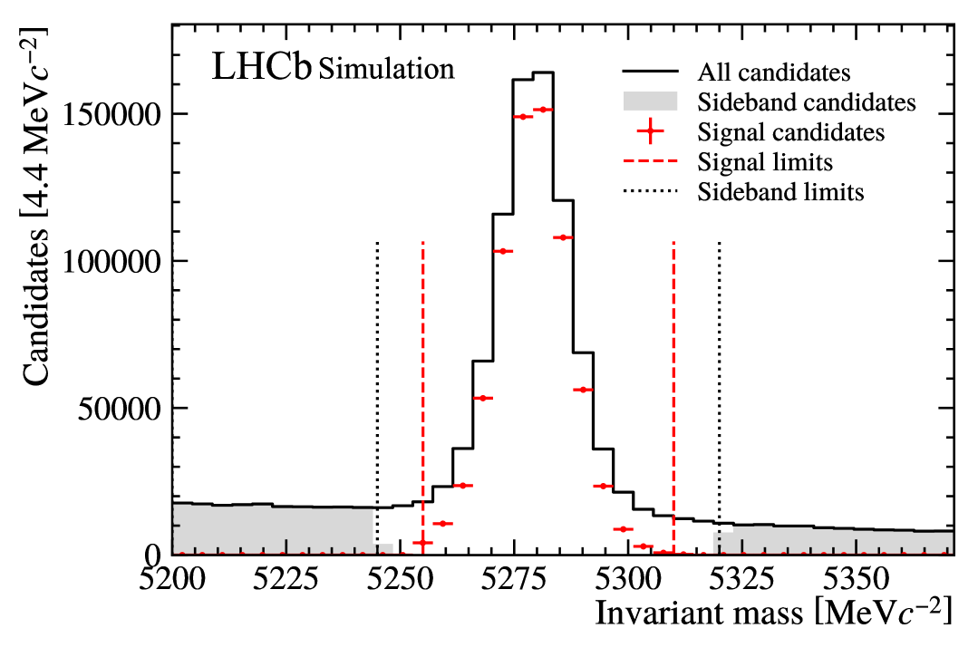
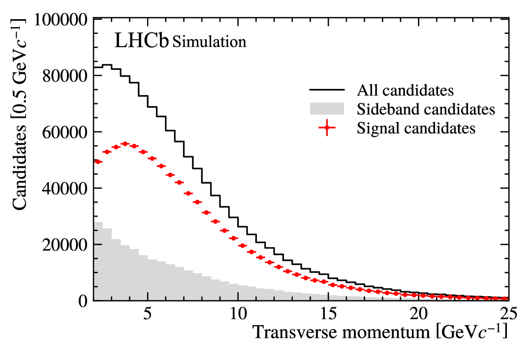
Figure 2: Distributions of (left) invariant mass and (right) transverse momentum for the ${{{B}^{+}}}\!\rightarrow{{J\mskip-3.0mu/\mskip-2.0mu\psi}}\left({\mu^{+}\mu^{-}}\right){{K}^{+}}$ decay sample. Signal and sideband regions used for sideband-subtraction are shown as red and black lines, respectively. Candidates falling within the sidebands are shown in grey, whilst the sideband-subtracted candidates are shown in red.

3.1.2 Fit-and-count

The fit-and-count method exploits extended probability density functions (PDFs) to describe the discriminating distribution of the decay of interest, to which a negative log-likelihood fit is performed. This approach allows analysts to define separate PDFs describing the signal and different possible backgrounds. As such, the fit-and-count method appropriately handles more complex background contributions. However, this approach relies on the stability of the likelihood fit, which can be problematic in phase-space regions with low number of events. A possible solution to this is presented in the next section through the sPlot approach. The TriggerCalib implementation of the method gives the flexibility to split the sample using different phase-space variables and regions.

In our validation study, the ${{{B}^{+}}}\!\rightarrow{{J\mskip-3.0mu/\mskip-2.0mu\psi}}\left({\mu^{+}\mu^{-}}\right){{K}^{+}}$ signal component is described by a double-sided Crystal Ball function [20], whilst combinatorial background is described by an exponential distribution. Parameters describing the signal are obtained from likelihood fits to truth-matched simulated samples, with the mean and width of the distribution left floating in fits to the full simulated sample with added background. Figure 3 shows the mass distribution of the ${{{B}^{+}}}\!\rightarrow{{J\mskip-3.0mu/\mskip-2.0mu\psi}}\left({\mu^{+}\mu^{-}}\right){{K}^{+}}$ sample for one example $p_{\mathrm{T}}$ bin, overlaid with the likelihood fit result.

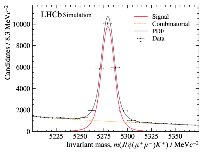
Figure 3: Distribution of the ${J\mskip-3.0mu/\mskip-2.0mu\psi}$ ${K}^{+}$ invariant mass distribution for a single $p_{\mathrm{T}}$ bin, overlaid with the results of the likelihood fit.

3.1.3 The sPlot method

As in the fit-and-count method, the sPlot method requires the definition of PDFs describing signal and background components. However, rather than fitting in each phase-space region, a global likelihood fit is performed to compute signal sWeights from the sPlot formalism [18]. The number of signal candidates in each $i$-th region of the phase space can then be evaluated as:

$$N_{i}=\sum\limits_{j}w_{j},$$ (3.2)

with $w_{j}$ the signal sWeight for each candidate $j$ which lies within region $i$.

The distributions of the $p_{\mathrm{T}}\left({{K}^{+}}{\mu^{+}}{\mu^{-}}\right)$ with sWeights for the signal and background components computed from a fit to $m\left({{J\mskip-3.0mu/\mskip-2.0mu\psi}}{{K}^{+}}\right)$ are shown in Figure 4.

Figure 4: Distributions of the ${{B}^{+}}$ transverse momentum with sWeights of the signal and combinatorial background components applied. These sWeights are calculated from a single likelihood fit to the entire ${{{B}^{+}}}\!\rightarrow{{J\mskip-3.0mu/\mskip-2.0mu\psi}}\left({\mu^{+}\mu^{-}}\right){{K}^{+}}$ sample.

The advantage of this approach is that only a single likelihood fit per category is sufficient to obtain all of the information required to evaluate the trigger efficiencies with the $\mathrm{TISTOS}$ method in regions of the phase space. This is in contrast to the fit-and-count method, in which many fits must be performed per category. However, the sPlot formalism is only valid if the variables of interest (control variables) are uncorrelated to the discriminating variable.

Correlations between control and discriminating variables could lead to a biased evaluation of the trigger efficiency. Two tests of this, proposed by the sweights package [21], are implemented in TriggerCalib: the likelihood ratio test and Kendall’s $\tau$ test.

The likelihood ratio test divides a sample into two regions in the control variable and tests a null hypothesis (components have the same shape in both subsamples) and an alternate hypothesis wherein the shape of components of the distribution depend on the control variable. This is tested by performing two likelihood fits: one ($H_{0}$) fitting a model simultaneously to both subsamples which shares shape parameters and the other ($H_{1}$) fitting independent PDFs to each subsample. From the resulting likelihoods, $L_{H_{0}}$ and $L_{H_{1}}$, respectively, a $Q$-statistic can be defined:

$$Q=-2\cdot(\ln\mathrm{sup}\{L_{H_{0}}\}-\ln\mathrm{sup}\{L_{H_{1}}\}).$$ (3.3)

A $p$-value is then obtained from a $\chi^{2}$ distribution with $N^{H_{1}}-N^{H_{0}}$ degrees of freedom, evaluated at the $Q$-statistic value.

Kendall’s $\tau$ test takes an alternative approach, using pure signal and background samples (which can typically be obtained from signal simulation and sideband data subsamples) for the components present in the discriminating distribution. For each subsample, the Kendall rank correlation coefficient, $\tau$, is computed between a control variable and the discriminating variable. This $\tau$ is used to perform a hypothesis test wherein the null hypothesis is that the variables are independent, i.e, $\tau=1$. As for the likelihood ratio test, a $p$-value is obtained from the hypothesis test which can be used to acce pt/reject the null hypothesis to a given confidence. The test is only passed if the null hypothesis holds for both the signal and background samples.

In our validation study, this means that the invariant mass of the ${{B}^{+}}$ candidates must be uncorrelated with the transverse/longitudinal momenta for the sWeights computed from global fits to be unbiased. Both of the tests described above were performed to probe the dependence between $m\left({{J\mskip-3.0mu/\mskip-2.0mu\psi}}{{K}^{+}}\right)$ and $p_{\mathrm{T}}\left({{K}^{+}}{\mu^{+}}{\mu^{-}}\right)$, laid out in Appendix C. Whilst the conclusion of these tests are that the two variables are not independent, if the bias in the sWeights affects each category ($\mathrm{TIS}$, $\mathrm{TOS}$, etc.) equally, then these effects may cancel in the computed efficiencies.

3.2 Data-driven trigger efficiencies

TriggerCalib allows the computation of data-driven trigger efficiencies in $n$-dimensional phase-space regions through the $\mathrm{TISTOS}$ method with Equation 2.5. The evaluation of the trigger efficiencies as a function of kinematic variables is also available. Furthermore, all three of the background mitigation approaches presented in the previous sections can be used to evaluate the trigger yields.

The sideband subtraction, fit-and-count and sPlot methods are compared for the ${{{B}^{+}}}\!\rightarrow{{J\mskip-3.0mu/\mskip-2.0mu\psi}}\left({\mu^{+}\mu^{-}}\right){{K}^{+}}$ sample with added background. Integrated trigger efficiencies are evaluated according to Equation 2.5, dividing the phase space into regions of the ${{B}^{+}}$ transverse and longitudinal momenta, and listed in Table 1. The phase space is divided into 5 bins of $p_{\mathrm{T}}\left({{K}^{+}}{\mu^{+}}{\mu^{-}}\right)\in\left[2,25\right]\text{\,Ge\kern-1.00006ptV\!/}c$. Bins are chosen to contain an approximately equal number of events in the $\mathrm{TISTOS}$ category, as this is the smallest component of Equation 2.5. All three efficiencies are consistent with one another, as expected for a well-understood control channel with well-behaved backgrounds such as ${{{B}^{+}}}\!\rightarrow{{J\mskip-3.0mu/\mskip-2.0mu\psi}}\left({\mu^{+}\mu^{-}}\right){{K}^{+}}$; however, this may not be generally true. The difference in sensitivity between the sideband subtraction and fit-and-count/sPlot methods arises entirely from uncertainties in fitting, and hence is dependent on the construction and quality of the fits to the discriminating variable.

Background mitigation approach	Trigger efficiency / $\%$
Sideband subtraction	$97.328\pm 0.054$
Fit-and-count (RooFit)	$97.31\pm 0.11$
Fit-and-count (zFit)	$97.31\pm 0.11$
sPlot (RooFit)	$97.314\pm 0.094$
sPlot (zFit)	$97.312\pm 0.094$

Table 1: Trigger efficiency evaluated on the ${{{B}^{+}}}\!\rightarrow{{J\mskip-3.0mu/\mskip-2.0mu\psi}}\left({\mu^{+}\mu^{-}}\right){{K}^{+}}$ simulated sample with the $\mathrm{TISTOS}$ method. Different background mitigation approaches are compared. The $\mathrm{TISTOS}$ method is applied splitting the sample regions of $p_{\mathrm{T}}$ and $p_{z}$ of the $B$ mesons. Accompanying uncertainties are purely statistical.

An additional comparison is made for the $p_{\mathrm{T}}$-dependent trigger efficiencies, shown for a one-dimensional binning of the sample in four $p_{\mathrm{T}}$ bins in Figure 5. As for the integrated trigger efficiencies, the trigger efficiencies in each bin are consistent for each of the three background mitigation approaches.

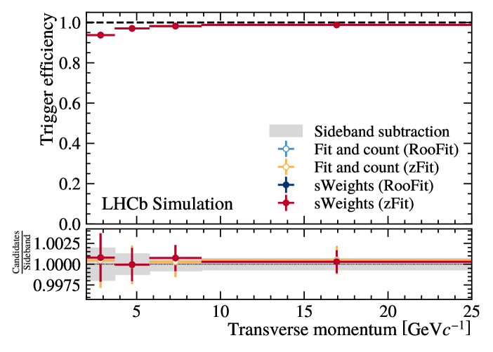
Figure 5: Trigger efficiency evaluated on the ${{{B}^{+}}}\!\rightarrow{{J\mskip-3.0mu/\mskip-2.0mu\psi}}\left({\mu^{+}\mu^{-}}\right){{K}^{+}}$ simulated sample as a function of the $p_{\mathrm{T}}$ of the $B^{+}$ meson candidate. The different background mitigation methods implemented in the TriggerCalib package are compared, using both the RooFit and zFit implementations (which return consistent results).

3.3 Data-simulation corrections

The TriggerCalib software package allows the calculation of correction weights to the trigger response of simulated samples. Such corrections can be computed in a well-understood process of high statistics and applied to rare or unobserved processes in which it is not possible to directly calculate trigger efficiencies from data. However, this method requires a control sample which is kinematically and topologically similar to the signal channel.

For example, this approach was used in the LHCb measurement of the lepton flavour universality ratios $R_{K}$ and $R_{K^{\ast}}$ in ${{{B}^{+}}}\!\rightarrow{{K}^{+}}\ell^{+}\ell^{-}$ and ${{B}^{0}}\!\rightarrow{{K}^{*0}}\ell^{+}\ell^{-}$ decays [22, 23] where the ${{{B}^{+}}}\!\rightarrow{{J\mskip-3.0mu/\mskip-2.0mu\psi}}\left(\ell^{+}\ell^{-}\right){{K}^{+}}$ decay was used as control channel.

For efficiencies computed in phase-space bins $i$, the correction weights are given by

$$w_{i}=\frac{\varepsilon^{\mathrm{data}}_{i}}{\varepsilon^{\mathrm{simulation}}_{i}},$$ (3.4)

with $\varepsilon^{\mathrm{data/simulation}}_{i}$ as efficiencies computed with the $\mathrm{TISTOS}$ method on a data/simulated sample in a phase-space region $i$.

4 Uncertainties

The uncertainties affecting the methods available in the TriggerCalib package are discussed in the following sections. Whilst the uncertainties on the efficiency calculation are generally treated as systematic uncertainties in analyses, the discussion here involves both statistical and systematic uncertainties for the aspects of the presented methods.

The TriggerCalib software does not directly compute the values of the systematic uncertainties on the methods, hence the discussion here focuses on describing their source and possible treatments. The correct approach to determine systematic uncertainties may vary from analysis to analysis, depending on the signal channel(s) under study and the analysis techniques.

4.1 Statistical uncertainties

Statistical uncertainties on the $\mathrm{TISTOS}$ method are typically lead by the limited size of the data sample(s) in use. The correct evaluation of the statistical uncertainty becomes more complex when splitting the dataset in phase-space regions and dealing with low number of events.

In particular, the variance on the denominator of $\varepsilon_{\mathrm{Trig.}}$ must be computed by decomposing its constituent parts into independent terms:

$$\varepsilon_{\mathrm{Trig.}}=\frac{N_{\mathrm{Trig.}}}{\sum\limits_{i}{\frac{\left(\alpha^{i}+\gamma^{i}\right)\left(\beta^{i}+\gamma^{i}\right)}{\gamma^{i}}}},$$ (4.1)

for terms $\alpha^{i}=N_{\mathrm{TIS}}^{i}-N_{\mathrm{TISTOS}}^{i}$, $\beta^{i}=N_{\mathrm{TOS}}^{i}-N_{\mathrm{TISTOS}}^{i}$ and $\gamma^{i}=N_{\mathrm{TISTOS}}^{i}$, which contain exclusively TIS, TOS and TISTOS events, respectively. As demonstrated in Ref. [16], the variance of the denominator, $\sigma_{N_{\mathrm{Tot.}}}^{2}$ can be expressed as

$$\sigma_{N_{\mathrm{Tot.}}}^{2} =\sum\limits_{i}{\sigma_{N_{\mathrm{Tot.}}^{i}}^{2}}$$

$$=\sum\limits_{i}{\left(\frac{\beta^{i}+\gamma^{i}}{\gamma^{i}}\right)^{2}\sigma_{\alpha^{i}}^{2}+\left(\frac{\alpha^{i}+\gamma^{i}}{\gamma^{i}}\right)^{2}\sigma_{\beta^{i}}^{2}+\left(1-\frac{\alpha^{i}\beta^{i}}{\left(\gamma^{i}\right)^{2}}\right)^{2}\sigma_{\gamma^{i}}^{2}.}$$ (4.2)

The variances $\sigma_{\alpha^{i}}^{2}$ and $\sigma_{\beta^{i}}^{2}$ are taken such that $\sigma_{N_{\mathrm{TIS}}^{i}}^{2}=\sigma_{\alpha^{i}}^{2}+\sigma_{N_{\mathrm{TISTOS}}^{i}}^{2}$ and $\sigma_{N_{\mathrm{TOS}}^{i}}^{2}=\sigma_{\beta^{i}}^{2}+\sigma_{N_{\mathrm{TISTOS}}^{i}}^{2}$, respectively.

The statistical uncertainty on $\varepsilon_{\mathrm{trig.}}$ is determined by means of a generalised Wilson interval, as defined in Ref. [24]. Defining an efficiency, $\hat{\varepsilon}$, in terms of pass and fail counts, $m_{1}$ and $m_{2}$, the variance on each count can be expressed as

$$\sigma_{m_{i}}^{2}=m_{i}+\sigma_{i,b}^{2},$$ (4.3)

wherein $m_{i}$ is a Poisson contribution and $\sigma_{i,b}^{2}$ is a non-Poisson contribution. The generalised Wilson interval given in Ref. [24] differs from the conventional Wilson interval [25] by incorporating the contributions $\sigma_{1,b}^{2}$ and $\sigma_{2,b}^{2}$.

Assuming that $\hat{n}_{i}$ describes $n_{i}$ well, the contributions $\sigma_{i,b}^{2}$ can be computed as

$$\sigma_{1,b}^{2}=\sigma_{N_{\mathrm{Trig.}}}^{2}-N_{\mathrm{Trig.}},$$ (4.4a)

$$\sigma_{2,b}^{2}=\sigma_{N_{\mathrm{Tot.}}}^{2}-N_{\mathrm{Tot.}},$$ (4.4b)

where $N_{\mathrm{Tot.}}$ and $\sigma_{N_{\mathrm{Tot.}}}^{2}$ are taken from Eqs. 4.1 and 4.2, respectively.

4.2 Systematic uncertainties

Systematic uncertainties on the data-driven trigger efficiency evaluation implemented in the TriggerCalib package may arise from the choices of:

• the channel of interest, typically referred to as a calibration mode, in which the efficiencies are computed,

• the phase-space variables and regions scheme,

• the trigger decisions used to select the tag sample,

• the background mitigation method.

The calibration mode should be chosen to be as representative as possible of the signal channel studied. The TriggerCalib software package supports the variation of the control mode which could lead to different values of the trigger efficiencies and be used as source of systematic uncertainty.

The choice on how the dataset is partitioned in regions of the decay phase space should balance a minimal statistical uncertainty (by choosing sufficiently large regions) and a minimal bias (by avoiding large regions as per Section 2.3). To evaluate a systematic uncertainty for the choice of binning, analysts must compute efficiencies under varied phase-space divisions. Furthermore, different phase-space variables can be tested to compute alternative values of the trigger efficiencies.

The trigger decisions chosen to select the tag sample in the $\mathrm{TISTOS}$ method may lead to different types of correlations between the tag and probe samples. These correlations are mitigated when computing efficiencies in smaller and smaller regions of the phase space, as discussed in Section 2.2. Systematic uncertainties on the trigger efficiency evaluation can be assigned by varying the tag trigger decisions while keeping the same phase-space division scheme.

The choice of background mitigation method may lead to subtly different results on the evaluation of the trigger efficiencies. No differences were shown in Section 3.2 for the ${{{B}^{+}}}\!\rightarrow{{J\mskip-3.0mu/\mskip-2.0mu\psi}}\left({\mu^{+}\mu^{-}}\right){{K}^{+}}$ samples. However, these samples are characterized by low-background and simple fit models. When studying different decay channels, the assumptions made during the studies performed in this paper may need further validation. Analysts can compute systematic uncertainties on the trigger efficiency evaluation by varying the background mitigation method used.

5 Conclusion

The TriggerCalib package facilitates the determination of LHCb trigger efficiencies and performance through a set of software tools. It implements calculations of the $\mathrm{TISTOS}$ method which make a fully data-driven efficiency determination possible. Furthermore, the package gives the possibility to apply corrections to the trigger response of simulated samples. This permits analysts to evaluate the trigger efficiency directly on simulation.

This paper covers, in detail, the functionalities of the TriggerCalib tooling, validating them with simulated ${{{B}^{+}}}\!\rightarrow{{J\mskip-3.0mu/\mskip-2.0mu\psi}}\left({\mu^{+}\mu^{-}}\right){{K}^{+}}$ decays in conditions equivalent to LHCb data-taking in 2024. Different background mitigation approaches have been presented and found to produce consistent results in these samples. All three approaches are implemented and available in the package to give full flexibility to analysts when calculating trigger efficiencies. Additionally, TriggerCalib allows the evaluation of trigger efficiencies in regions of the signal phase space to study dependencies of the trigger response and control the validity of the $\mathrm{TISTOS}$ method. A discussion on the uncertainties of the methods is carried out in the last section and their computation may depend on the type of analysis performed. Generally, the main systematic uncertainty is related to correlations between the trigger response and the kinematics of the signal channel.

In conclusion, the scope of the TriggerCalib software package is to provide a centralised implementation of calculations of LHCb trigger efficiency and performance, giving analysts the possibility to exploit the available tools with great flexibility.

Appendix A Background model

To provide a background to the MC generated sample of ${{{B}^{+}}}\!\rightarrow{{J\mskip-3.0mu/\mskip-2.0mu\psi}}\left({\mu^{+}\mu^{-}}\right){{K}^{+}}$ decays, toy candidates were generated. This background component was constructed to mimic a typical combinatorial background, with an exponential shape in the ${J\mskip-3.0mu/\mskip-2.0mu\psi}$ ${K}^{+}$ invariant mass and ${K}^{+}$ $\mu^{+}$ $\,\upmu\text{m}$ transverse momentum distributions, using exponents of $\ell_{m}=5\times 10^{-3}\left(\text{\,Me\kern-1.00006ptV\!/}c^{2}\right)^{-1}$ and $\ell_{p_{T}}=2\times 10^{-4}{\left(\text{\,Me\kern-1.00006ptV\!/}c\right)}^{-1}$, respectively.

Taking the fraction of events in the simulated ${{{B}^{+}}}\!\rightarrow{{J\mskip-3.0mu/\mskip-2.0mu\psi}}\left({\mu^{+}\mu^{-}}\right){{K}^{+}}$ sample with a $\mathrm{TIS}$/$\mathrm{TOS}$ decision for each HLT1 line, $i$, as $f^{i}_{\mathrm{TIS}(\mathrm{TOS})}$, each candidate in the background sample was assigned a $\mathrm{TIS}$/$\mathrm{TOS}$ decision based on a number drawn from a uniform random variable on $n=\left[0,1\right]$. The candidate was labelled $\mathrm{TIS}$ for a given line if $n<f^{i}_{\mathrm{TIS}}$ and $\mathrm{TOS}$ if $n<f^{i}_{\mathrm{TOS}}/2$, with $n$ redrawn for each decision.

Appendix B The implementation of TriggerCalib

TriggerCalib has been implemented as a standalone Python package, hosted on the CERN GitLab at https://gitlab.cern.ch/lhcb-rta/triggercalib and deployed to PyPI at https://pypi.org/project/triggercalib/. The documentation of the package, which contains a user guide, tutorials and a full reference of the package contents, can be found at https://triggercalib.docs.cern.ch/. The package is built upon functionality of the Root data analysis framework [26], producing Root histogram and graph objects which analysts can manipulate directly or save for later use, e.g., to take the ratio of efficiencies to produce corrections to simulation.

The likelihood fit functionality required by the fit-and-count and sPlot background mitigations (discussed in Sections 3.1.2 and 3.1.3, respectively), and the likelihood test of sWeight factorisation (discussed in Section. C) is implemented through both RooFit [27] and zFit [28] fitting libraries. This functionality accepts a user-defined observable and probability density function from either library, and performs fits via the corresponding library.

Appendix C sWeight factorisation tests

The likelihood test described in Section 3.1.3 was performed on the ${{{B}^{+}}}\!\rightarrow{{J\mskip-3.0mu/\mskip-2.0mu\psi}}\left({\mu^{+}\mu^{-}}\right){{K}^{+}}$ simulated sample with generated background, performing fits to the ${{J\mskip-3.0mu/\mskip-2.0mu\psi}}{{K}^{+}}$ invariant mass and dividing the sample equally in $p_{\mathrm{T}}\left({{K}^{+}}{\mu^{+}}{\mu^{-}}\right)$. The mean and width of the signal and exponent of the combinatorial were shared between subsamples in the $H_{0}$ case and floated separately in the $H_{1}$ case. Their values, the yields in each subsample and the corresponding minimised negative-log likelihood values are listed in Table 2. These yield a $Q$-statistic of $269.3$, corresponding to a $p$-value of $4.3\times 10^{-58}$ for the 3 degrees of freedom differing between $H_{0}$ and $H_{1}$. The null hypothesis $H_{0}$, that the ${{J\mskip-3.0mu/\mskip-2.0mu\psi}}{{K}^{+}}$ invariant mass and $p_{\mathrm{T}}\left({{K}^{+}}{\mu^{+}}{\mu^{-}}\right)$ are independent, is therefore rejected. This conclusion is particularly evident when comparing the signal widths between the low- and high-$p_{\mathrm{T}}$ fits for $H_{0}$, where these differ by $\left(0.497\pm 0.022\right)\text{\,Me\kern-1.00006ptV}$.

The Kendall $\tau$ test was also performed, taking MC simulated ${{{B}^{+}}}\!\rightarrow{{J\mskip-3.0mu/\mskip-2.0mu\psi}}\left({\mu^{+}\mu^{-}}\right){{K}^{+}}$ events as the signal sample and events from the background generated according to Appendix A as the background sample. The results of this test are listed in Table 3. For a confidence of 99.7%, $m\left({{J\mskip-3.0mu/\mskip-2.0mu\psi}}{{K}^{+}}\right)$ and $p_{\mathrm{T}}\left({{K}^{+}}{\mu^{+}}{\mu^{-}}\right)$ can be considered independent in the background sample only.

Quantity	Simultaneous fit, $H_{0}$		Separate fits, $H_{1}$
	Low $p_{\mathrm{T}}$	High $p_{\mathrm{T}}$	Low $p_{\mathrm{T}}$	High $p_{\mathrm{T}}$
Signal mean, $\mu$ /  MeV	$5279.460\pm 0.011$		$5279.480\pm 0.016$	$5279.450\pm 0.016$
Signal width, $\sigma$ /  MeV	$7.365\pm 0.011$		$7.586\pm 0.015$	$7.089\pm 0.016$
Combinatorial exponent, $\ell$ / $10^{-3}\text{\,Me\kern-1.00006ptV}^{-1}$	$\left(-4.932\pm 0.016\right)\times 10^{-3}$		$\left(-4.901\pm 0.023\right)\times 10^{-3}$	$\left(-4.966\pm 0.021\right)\times 10^{-3}$
Signal yield	$331130\pm 660$	$384320\pm 700$	$386920\pm 670$	$328050\pm 700$
Combinatorial yield	$349710\pm 670$	$296520\pm 630$	$352790\pm 690$	$293922\pm 640$
Negative log-likelihood, $-2\ln\sup\left\{L_{H_{i}}\right\}$	-9173670.41		-9188431.25
$Q$-statistic	269.3
$p$-value	$4.3\times 10^{-58}$

Table 2: Results of the likelihood-ratio factorisation test.

Quantity	Signal (MC simulation)	Background (per Appendix A)
$\tau$ coefficient	$\left(1.151\pm 0.077\right)\times 10^{-2}$	$\left(6.4\pm 7.2\right)\times 10^{-3}$
$p$-value	$1.1\times 10^{-50}$	$0.37$

Table 3: Results of the Kendall $\tau$ test.

References

- [1] LHCb collaboration, The LHCb detector at the LHC, JINST 3 (2008) S08005.
- [2] LHCb collaboration, LHCb detector performance, Int. J. Mod. Phys. A30 (2015) 1530022 LHCB-DP-2014-002, CERN-PH-EP-2014-290, [1412.6352].
- [3] LHCb collaboration, The LHCb Upgrade I, JINST 19 (2024) P05065 LHCb-DP-2022-002, [2305.10515].
- [4] LHCb collaboration, A Comparison of CPU and GPU Implementations for the LHCb Experiment Run 3 Trigger, Comput. Softw. Big Sci. 6 (2022) 1 [2105.04031].
- [5] A. Mathad, M. Ferrillo, S. Barré, P. Koppenburg, P. Owen, G. Raven et al., FunTuple: A New N-tuple Component for Offline Data Processing at the LHCb Experiment, Comput. Softw. Big Sci. 8 (2024) 6 [2310.02433].
- [6] N. Skidmore, E. Rodrigues and P. Koppenburg, Run-3 offline data processing and analysis at LHCb, PoS EPS-HEP2021 (2022) 792.
- [7] T. Sjöstrand, S. Mrenna and P. Skands, A brief introduction to PYTHIA 8.1, Comput. Phys. Commun. 178 (2008) 852 [0710.3820].
- [8] T. Sjöstrand, S. Mrenna and P. Skands, PYTHIA 6.4 physics and manual, JHEP 05 (2006) 026 [hep-ph/0603175].
- [9] I. Belyaev et al., Handling of the generation of primary events in Gauss, the LHCb simulation framework, J. Phys. Conf. Ser. 331 (2011) 032047.
- [10] D.J. Lange, The EvtGen particle decay simulation package, Nucl. Instrum. Meth. A462 (2001) 152.
- [11] N. Davidson, T. Przedzinski and Z. Was, PHOTOS interface in C++: Technical and physics documentation, Comp. Phys. Comm. 199 (2016) 86 [1011.0937].
- [12] Geant4 collaboration, Geant4 developments and applications, IEEE Trans.Nucl.Sci. 53 (2006) 270.
- [13] Geant4 collaboration, Geant4: A simulation toolkit, Nucl. Instrum. Meth. A506 (2003) 250.
- [14] M. Clemencic et al., The LHCb simulation application, Gauss: Design, evolution and experience, J. Phys. Conf. Ser. 331 (2011) 032023.
- [15] R. Aaij et al., The LHCb trigger and its performance in 2011, JINST 8 (2013) P04022 LHCb-DP-2012-004, [1211.3055].
- [16] S. Tolk, J. Albrecht, F. Dettori and A. Pellegrino, Data driven trigger efficiency determination at LHCb, 2014.
- [17] R. Aaij et al., Design and performance of the LHCb trigger and full real-time reconstruction in Run 2 of the LHC, JINST 14 (2019) P04013 [1812.10790].
- [18] M. Pivk and F.R. Le Diberder, sPlot: A statistical tool to unfold data distributions, Nucl. Instrum. Meth. A555 (2005) 356 [physics/0402083].
- [19] Particle Data Group collaboration, Review of particle physics, Prog. Theor. Exp. Phys. 2022 (2022) 083C01.
- [20] T. Skwarnicki, A study of the radiative cascade transitions between the Upsilon-prime and Upsilon resonances, Ph.D. thesis, Institute of Nuclear Physics, Krakow, 1986.
- [21] H. Dembinski, M. Kenzie, C. Langenbruch and M. Schmelling, Custom Orthogonal Weight functions (COWs) for event classification, Nucl. Instrum. Meth. A 1040 (2022) 167270 [2112.04574].
- [22] LHCb collaboration, Measurement of lepton universality parameters in and decays, Phys. Rev. D108 (2023) 032002 LHCb-PAPER-2022-045,CERN-EP-2022-278, [2212.09153].
- [23] LHCb collaboration, Test of lepton universality in decays, Phys. Rev. Lett. 131 (2023) 051803 LHCb-PAPER-2022-046,CERN-EP-2022-277, [2212.09152].
- [24] H. Dembinski and M. Schmelling, Bias, variance, and confidence intervals for efficiency estimators in particle physics experiments, 2110.00294.
- [25] E.B. Wilson, Probable Inference, the Law of Succession, and Statistical Inference, J. Am. Statist. Assoc. 22 (1927) 209.
- [26] R. Brun and F. Rademakers, ROOT: An object oriented data analysis framework, Nucl. Instrum. Meth. A 389 (1997) 81.
- [27] W. Verkerke and D.P. Kirkby, The RooFit toolkit for data modeling, eConf C0303241 (2003) MOLT007 [physics/0306116].
- [28] J. Eschle, A.N. Puig, R. Silva Coutinho and N. Serra, zfit: scalable pythonic fitting, EPJ Web Conf. 245 (2020) 06025.