Gaussian Processes in Power Systems: Techniques, Applications, and Future Works

Abstract

The increasing integration of renewable energy sources (RESs) and distributed energy resources (DERs) has significantly heightened operational complexity and uncertainty in modern power systems. Concurrently, the widespread deployment of smart meters, phasor measurement units (PMUs) and other sensors has generated vast spatiotemporal data streams, enabling advanced data-driven analytics and decision-making in grid operations. In this context, Gaussian processes (GPs) have emerged as a powerful probabilistic framework, offering uncertainty quantification, non-parametric modeling, and predictive capabilities to enhance power system analysis and control. This paper presents a comprehensive review of GP techniques and their applications in power system operation and control. GP applications are reviewed across three key domains: GP-based modeling, risk assessment, and optimization and control. These areas serve as representative examples of how GP can be utilized in power systems. Furthermore, critical challenges in GP applications are discussed, and potential research directions are outlined to facilitate future power system operations.

I Introduction

The extensive reliance on fossil fuels has drastically elevated carbon emissions, presenting a substantial threat to global climate stability and sustainable development. As the principal medium for energy production and transmission, power systems are positioned at the forefront of the energy transition, playing an indispensable role in global carbon reduction efforts [1]. This transition has catalyzed the widespread adoption of renewable energy sources (RESs), distributed energy resources (DERs), and flexible loads, such as electric vehicles (EVs) [2]. While these components contribute to decarbonization, they simultaneously introduce considerable uncertainties and volatilities, posing challenges to the secure operation of power systems. Furthermore, as these elements are primarily integrated into the grid through power electronic devices, the overall system complexity is substantially increased, complicating both structural and parametric aspects of system modeling. Consequently, physics-based power system analyses may become either time-intensive or imprecise in the face of such uncertainties and complexities.

The proliferation of advanced sensing technologies, such as phasor measurement units (PMUs), smart meters, Internet of Things-related sensors, etc, has resulted in power systems generating more comprehensive and valuable data than ever before. This evolution is propelling power systems into a new era of digitalization and intelligence, offering a promising avenue for addressing the aforementioned challenges. As a result, there is a growing demand for data-driven analytical methods that not only extract critical steady-state and dynamic insights from data, but also improve the accuracy of physical system modeling.

A variety of machine learning (ML) techniques have been introduced for power system analysis, including shallow learning methods such as support vector machines (SVM) [3], as well as newer deep learning models like Transformer [4]. These approaches offer the advantage of being model-free and capable of generalizing to new power system scenarios, providing a degree of adaptability. However, learning models solely on data makes them prone to overfitting or incorporating unwanted biases, especially when the dataset is small [5]. To address these limitations, Bayesian methods have been developed to integrate prior knowledge into model learning. Of particular note is the framework of GP, an important Bayesian learning paradigm, that generalizes multivariate Gaussian distributions by placing distributions over functions [6, 7]. This enables GP to uncover hidden functional relationships in power system tasks when sufficient observations are collected. GP offers several key advantages that make it feasible for use in the analysis of critical infrastructure such as power systems, where safety is a priority.

• Flexible expressivity. The nonparametric nature of GP allows it to model highly complex functions [8], making it ideal for capturing the intricate dynamics of modern power systems, which may include complex devices with proprietary internal control structures, such as inverter-based resources (IBRs).

• Well-calibrated uncertainty quantification. A key advantage of GP is its ability to provide closed-form uncertainty estimates, accounting for both data noise and discrepancies from new scenarios that differ from the training data distribution [8]. This is essential for use within safety-critical systems such as power grids.

• Efficient with small datasets. By using Bayesian learning principles [7] and with only a few hyperparameters to optimize, GP models can generalize effectively even with limited data [9], which is particularly beneficial for applications where training data is scarce. Additionally, GP training can be interlaced with active learning [10] to overcome data scarcity if generating data is expensive and time-consuming.

Due to these advantages, GP has garnered increasing attention in the field of power systems in recent years, particularly for applications such as forecasting, risk analysis, and decision-making. This article presents the fundamentals of GP modeling and then explores its use cases in power grid analysis. To the best of our knowledge, this paper is the first to provide a comprehensive survey of GP applications in power systems. In addition, we discuss the key challenges and future directions for the use of GP in this field, as well as their integration with other data-driven methods. The main contributions of this paper are summarized as follows:

• This paper presents a comprehensive and structured overview of the fundamental concepts of GP, along with an overview of the supporting software ecosystem.

• This paper highlights key applications of GP in power systems, including load and renewable energy forecasting, power system static and dynamic modeling, risk assessment, and decision-making. The application procedures and prior work are discussed in detail, demonstrating how GP effectively addresses challenges in these domains.

• This paper investigates the major challenges in applying GP to power systems, such as scalability and robustness, and discusses applications where GP may have greater applicability. Lessons learned are discussed and finally, future research directions, particularly in integrating GP with other advanced data-driven methods, are outlined.

The remainder of this paper is organized as follows. Section II offers an overview of the fundamental principles and ecosystem of GP. Section III provides a comprehensive review of GP-based learning in power system applications: forecasting, static and dynamic estimation and solutions to optimization problems. Next, we show how such learned models can be used for static and dynamic risk assessment in power grids in Section IV, and inside optimization and control modules in Section V. Finally, Section VI discusses the challenges and proposes future research directions for the application of GP in power systems. Section VII concludes the paper.

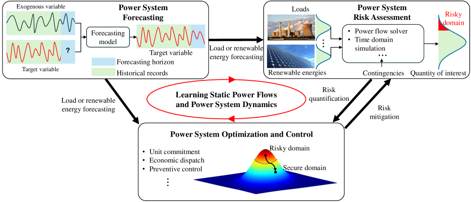
Figure 1: Illustration of GP applications across various domains of power systems. GP-based learning techniques have been used to support load and renewable energy forecasting, static and dynamic modeling of power flows, and are integrated into power system optimization and control. These methods further contribute to power system risk assessment through improved forecasting, risk quantification, and mitigation strategies, enhancing secure and reliable grid operation. See Table IV and Table V for specific works related to specific problems.

II Preliminaries of Gaussian Process

II-A Gaussian Process Fundamentals

This section presents the basic details of GP from a functional space perspective. GP is a non-parametric and probabilistic modeling method. Consider a latent function $f(\cdot)$ that describes a data point $(x_{i},y_{i})$ as follows:

$$y_{i}=f(x_{i})+\varepsilon_{i},$$ (1)

where $y_{i}$ is the observation with respect to the input $x_{i}$ of $i$-th sample, and $\varepsilon_{i}$ is a sample drawn from a Gaussian noise of zero mean and variance $\sigma^{2}_{\varepsilon}$.

Let, the function values $\bm{f}(x)=[f(x_{1}),f(x_{2}),\dots f(x_{N})]^{\top}$ for $N$ inputs $x=(x_{1},x_{2},\dots x_{k})$ be random values that are jointly Gaussian, i.e.,

$$\bm{f}(x)\sim\mathcal{N}(\bm{m}(x),K(x,x^{\prime})),$$ (2)

where $m(x)$ and $K(x,x)$ are the parameterized mean vector and covariance matrix, respectively, that depend on $x$. For example, for two input points, Gaussianity implies

$$\begin{bmatrix}f(x_{1})\\ f(x_{2})\end{bmatrix}\sim\mathcal{N}\bigg{(}\underbrace{\begin{bmatrix}m(x_{1})\\ m(x_{2})\end{bmatrix}}_{\texttt{Mean}},\underbrace{\begin{bmatrix}k(x_{1},x_{1})&k(x_{1},x_{2})\\ k(x_{2},x_{1})&k(x_{2},x_{2})\end{bmatrix}}_{\texttt{Covariance Matrix}}\bigg{)}.$$ (3)

By definition [7, 11],

A Gaussian Process is a (potentially infinite) collection of random variables such that any finite subset of it has a joint multivariate Gaussian distribution.

$f$ is termed a GP, denoted as $f\sim\mathcal{GP}(m,k)$. The distribution $\mathbb{P}(y)$ of the observation $y$ at inputs $x$ is given by marginalizing out $f$ to give

$$\mathbb{P}(y)=\int\mathbb{P}(y|f)d\mathbb{P}(f)\sim\mathcal{N}(m(x),K(x,x^{\prime})+\sigma_{\epsilon}^{2}\mathbb{I}).$$ (4)

The covariance matrix $K$ is composed of entries $K_{ij}=k(x_{i},x_{j})$ that measure the covariance of $f$ at two inputs $x_{1}$ and $x_{2}$. Both the mean and covariance function can be selected to encode prior knowledge about the shape of $f(\cdot)$. The Gaussianity of $f(x)$ and consequently of $y$ has a particularly attractive property, based on the efficient computation of conditional probability for Gaussian random variables. Consider that we want to determine the value of the function at a new input point $x^{\star}$. From the joint Gaussianity property, we know that observed values $y$ at training points and the new function value $f^{\star}$ is given by:

$$\begin{bmatrix}\bm{y}\\ f^{\star}\end{bmatrix}\sim\mathcal{N}\bigg{(}\begin{bmatrix}\bm{m}(x)\\ m(x^{\star})\end{bmatrix},\begin{bmatrix}K(x,x)+\sigma^{2}_{\varepsilon}\mathbb{I}&K(x,x^{\star})\\ K(x^{\star},x)&K(x^{\star},x^{\star})\end{bmatrix}\bigg{)}$$ (5)

where, $x$ is the vector of all input data points (training dataset) that we want to use for conditioning, $\mathbb{I}$ denotes a identity matrix, $K(x,x)$ is the covariance matrix among training points, $K(x,x^{\star})$ is the covariance between training points and a new input point, and $K(x^{\star},x^{\star})$ is the self-covariance of the new input point. As conditioning on training data implies that we want to know the value of $f^{\star}$ given $y$, we can use the Gaussian distribution conditioning result to obtain the distribution of $f^{\star}$, as given in (6).

$$f^{\star}|\bm{y}\sim \mathcal{N}\Big{(}m(x^{\star})+K(x^{\star},x)\big{[}K(x,x)+\sigma^{2}_{\varepsilon}\mathbb{I}\big{]}^{-1}(\bm{y}-\bm{m}(x)),K(x^{\star},x^{\star})-K(x^{\star},x)\big{[}K(x,x)+\sigma^{2}_{\varepsilon}\mathbb{I}\big{]}^{-1}K(x,x^{\star})\Big{)}.$$ (6)

The mean and covariance functions are parameterized to adapt the GP model based on the training data. These parameters are referred to as hyperparameters. Table I shows a few commonly used covariance/kernel functions and their associated hyperparameters. A standard strategy is often to use a mean function of zero. To learn these hyperparameters from the training data, one can use maximum log-likelihood on the marginal distribution $\mathbb{P}(y)$ of observations $y$ at inputs $x$, as:

$$-\frac{1}{2}\big{[}\bm{y}^{\top}[K+\sigma^{2}_{\varepsilon}\mathbb{I}]\bm{y}+\log|K+\sigma^{2}_{\varepsilon}\mathbb{I}|+N\log 2\pi\big{]}.$$ (7)

Fig. 2 shows the prediction comparison among linear, polynomial, and GP regressions on the sine function with added noise. All models are trained using only 10 observations. While the linear and polynomial models provide point estimates with limited flexibility, the GP regression not only captures the nonlinear pattern of the data more accurately but also quantifies predictive uncertainty through variance estimates, providing confidence intervals around its predictions. This demonstrates the advantages of GP in modeling complex nonlinear relationships and evaluating the reliability of its outputs.

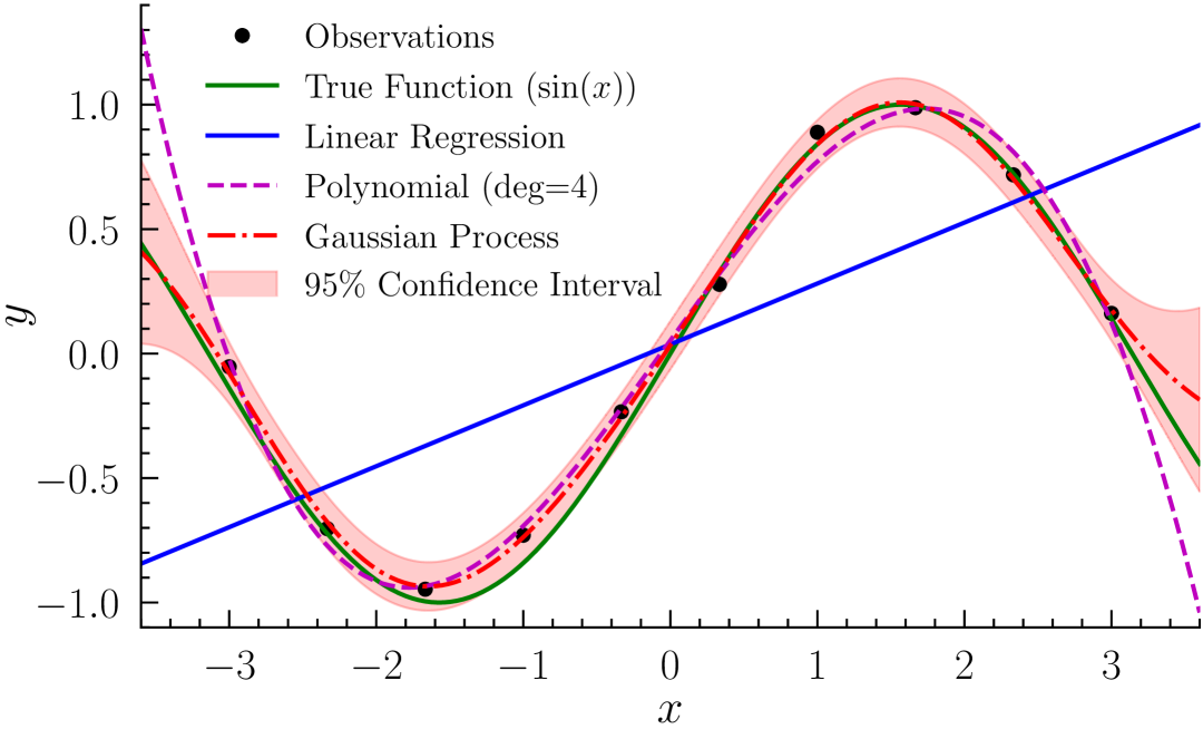
Figure 2: Comparison of linear, polynomial, and GP regressions (using Square Exponential kernel with $\nu^{2}=1$) on $y=\sin(x)+0.05\cdot\varepsilon$, where $\varepsilon\sim\mathcal{N}(0,1)$. Importantly, confidence interval information is only available with GP regression.

TABLE I: Standard Kernels for GP

Kernel Name	Function $k(x,x^{\prime})$
Linear	$\nu^{2}(x\cdot x^{\prime})$
Polynomial	$(\alpha(x\cdot x^{\prime})+c)^{d}$
Square Exponential	$\nu^{2}\exp\left(-\frac{\|x-x^{\prime}\|^{2}}{2l^{2}}\right)$
Matérn	$\frac{2^{1-\nu}}{\Gamma(\nu)}\left(\frac{\sqrt{2\nu}\|x-x^{\prime}\|}{l}\right)^{\nu}K_{\nu}\left(\frac{\sqrt{2\nu}\|x-x^{\prime}\|}{l}\right)$

• Hyperparameters– $\nu^{2}$: variance; $\alpha$: scale; $c$: offset; $d$: degree; $l$: length scale; $\nu$: smoothness. See Chapter 4 of [7] for more details.

TABLE II: Comprehensive Comparison of Selected GP Software Packages

Package	Language	GPU Support	Deep Learning	Maintenance	Package	Language	GPU Support	Deep Learning	Maintenance
GPy	Python	✓	✓(Basic)	Active	scikit-learn GP	Python	✗	✗	Active
GPflow	Python	✓	✓(Basic)	Active	PyMC3	Python	✗	✗	Active
GPyTorch	Python	✓	✓(Full)	Active	BoTorch	Python	✓	✓(Full)	Active
Pyro	Python	✓	✓(Full)	Active	GPML	MATLAB	✗	✗	✗

• Deep Learning: Full = Deep kernel learning (DKL) [12, 13] + Deep GP; Basic = Simple neural network integration.

• Maintenance: Active (Regular updates); Inactive (No updates in past 2 years).

Relation to non-linear Bayesian regression: The expressions of GP, including those between training and new data, can be derived by considering a Bayesian non-linear regression model $y=\Phi(x)\beta+\epsilon$, for a non-linear feature vector $\Phi(x)$, Gaussian noise $\epsilon$ and parameter vector $\beta$ that follows a Gaussian prior distribution. If $\Phi(x)$ is defined by a covariance matrix $K(x,x)$, similar expressions for posterior distribution of $y$ and $\Phi(x^{*})$ given training data $x$ can be derived by a MAP (Maximum APosteriori) estimator for $\beta$ using properties of Gaussian random variables and standard identities for matrix manipulation [7].

II-B Gaussian Process Ecosystem

A wide range of GP libraries have been extensively developed across various programming languages, including Python, MATLAB, Julia, and R. In MATLAB, the GPML package associated with the GP book [7] provides an excellent starting point for learning GP workings. GP libraries in the Python ecosystem, such as GPflow [14] and GPyTorch [15], offer significant advantages in deep learning integration and GPU acceleration, making them particularly suitable for uncertainty analysis and large-scale spatiotemporal data modeling. Also, BoTorch [16] provides necessary support for Bayesian Optimization using GP, along with large-scale GP regression. Further, Julia has several packages for working with GP, including KernelFunctions.jl, GPLikelihoods.jl, AbstractGPs.jl, and ApproximateGPs.jl. A few of these packages have been summarized in Table II.

III Gaussian Process based Modeling in Power System

In this section, we present four specific power system use-cases where GP has been directly used for modeling or learning.

III-A Forecasting: Loads and Renewable Energy Generation

The objective of load and renewable energy forecasting is to predict future power consumption and generation, both of which are essential for the efficient operation and strategic planning of power systems [17]. Based on the time horizon, power system forecasting tasks can be divided into four categories: ultra-short-term, short-term, medium-term, and long-term forecasting [18, 19]. The application scenarios differ across these time scales, as summarized in Table III, which provides a comparison of forecasting tasks for each horizon. Since ultra-short-term and short-term forecasting are important for energy management and real-time operations of power systems, the majority of research has concentrated on these two forecasting horizons [18].

Problem formulation: The forecasting model is developed to capture the relationship between historical data and future outcomes, and can be formulated as:

$$\hat{y}_{t+k|t}=f(\bm{x}_{t}|\bm{\theta}_{\text{forecast}}),$$ (8)

where $\hat{y}_{t+k|t}$ represents the targeted prediction at time $t+k$; $f$ denotes the forecasting function; $\bm{x}_{t}$ is the historical information vector, which may include indicators such as calendar time and weather data relevant to $\hat{y}_{t+k|t}$; and $\bm{\theta}$ denotes the hypeparameters of the forecasting model. Note that the output for solar can be either solar photovoltaic (PV) generation power or solar irradiance, with the latter being converted into PV generation power using a conversion function [18]. Similarly, wind forecast output can be either wind power generation or wind speed, with the latter being converted into wind power generation using the following conversion function [20]. The vector $\bm{x}_{t}$ can include historical records of the target variable $y$ and exogenous variables $\bm{z}$ as well as forecasts of $\bm{z}$.

Numerous machine learning methods have been used for forecasting load and renewable energy [21], including new Long Short-Term Memory Networks (LSTM) [22] and temporal convolutional networks [23]. Renewables such as wind and solar depend on variable and chaotic weather conditions [24], while power loads are impacted by weather and additional factors such as calendar effects, socioeconomic conditions [25]. As point forecasting methods may not adequately capture uncertainties, we discuss the use of GP-based forecasting in this area.

GP-based forecasting: Under the GP framework, the target variable values can be modeled as Gaussian-distributed realizations of $\hat{y}_{t}$ [26]:

$$y_{t+k|t} \sim\mathcal{N}\left(\hat{y}_{t+k|t},K(\bm{x}_{t},\bm{x}_{t}^{\prime})+\sigma_{\epsilon}^{2}\mathbb{I}\right),$$ (9)

$$\text{where}\quad\hat{y}_{t+k|t} =m\left(\bm{x}_{t}\mid\bm{\theta}_{\text{forecast}}\right).$$ (10)

As described in the previous section, $m$ is the mean function of $f$, $K$ represents the covariance function of the GP, $\mathbb{I}$ represents an identity matrix, and $\sigma^{2}_{\varepsilon}$ denotes observation noise. Here, $\sigma^{2}_{\varepsilon}$ reflects aleatoric uncertainty (due to measurement errors), while $K$ reveals epistemic uncertainty (due to error in forecasting model).

TABLE III: Application Scenarios of Load and Renewable Energy Forecasting in Different Time Scales

Time Scale (Forecast Range)	Application Scenarios
Ultra-short-term (Seconds to minutes)	Power system frequency control Real-time storage regulation
Short-term (few hours to days)	Day-ahead dispatch Backup optimization Unit commitment optimization
Medium-term (One week to months)	Maintenance plan
Long-term (Seasons or years)	Substation planning and selection Long-term generation plan Design of renewable integration

An example of load forecasting using a GP model is illustrated in Fig. 3. The training dataset comprises 12260 samples, each described by eight input features, including historical power consumption and temperature data with a 3-hour time lag. The training period spans from March 21, 2021, to August 13, 2022, covering diverse load consumption patterns. The GP model employs a squared exponential kernel with $\nu^{2}=1$ and is trained over 50 iterations. For evaluation, data from August 13, 2022, to March 20, 2023, is used. Fig. 3 specifically depicts forecasts for five days in August 2022. An extensive list of papers on enhanced GP-based forecasting tools for different time-scales as per Table III, is provided in Table IV along with the particular type of method used.

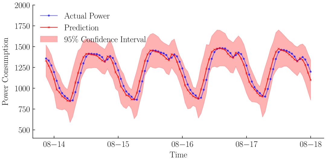
Figure 3: Load forecasting example using GP with squared exponential kernel.

TABLE IV: GP Applications in Power System Forecasting

Categories	Problems	References	Methodologies	Key Features
Forecasting feature engineering	Short-term wind speed forecasting	[27, 28]	Standard GP with Student-t observation model [27], Standard GP [28]	Wavelet transform is employed to extract relevant features from the input data.
	Short-term solar radiation forecasting	[29],[30]	Standard GP
	Short-term PV power forecasting	[31]	Standard GP	GP is integrated into a binary genetic algorithm framework to identify optimal input parameters.
	Wind speed forecasting	[32]	Standard GP	Shared-weight LSTM is used to extract the features of input data.
	Short-term wind power forecasting	[33]	Censored GP	ARD kernel is utilized to construct the covariance matrix of the GP, allowing for the calculation of each variable’s sensitivity during model learning.
	Short-term load forecasting	[34]	Standard GP
	Short-term load forecasting	[35]	Sparse heteroscedastic GP
	Short-term power consumption, PV power and net demand forecasting	[36]	Standard GP
Forecasting model enhancement	Short-term wind power forecasting	[37]	Sparse Variational GP	Variational sparse techniques leverage a reduced set of inducing points to approximate the full historical dataset, enabling efficient computation.
	Short-term load forecasting	[38], [39]	Sparse Variational GP [38], Multi-output sparse GP [39]
	Short-term wind speed forecasting	[40], [41]	Sparse Variational GP
	Short-term wind speed forecasting	[42]	Standard GP	An autoregressive model is utilized as the mean function of the GP to capture the overall structure of the wind speed time series.
	Short-term load forecasting	[43]	Standard GP	Composite covariance kernel functions are used to capture specific data characteristics, such as periodicity and local variability.
	Short-term solar radiation forecasting	[44]	Standard GP
	Short-term load forecasting	[45], [46], [47]	Deep GP [45], deep kernel learning [46], neural network GP [47]	End-to-end learning architectures, such as hierarchical GP structures or embedding neural networks into the kernel, are employed to enhance the expressiveness of GP.
Forecasting output functionality	Short-term load forecasting	[17]	Quantile GP	Deliver quantile predictions for load along with its associated probability density distribution
	Short-term wind power forecasting	[48]	Heteroscedastic GP	Automatically quantify time-varying noise in wind turbine power time series, using an adaptive noise variance updating mechanism.
	Short-term wind power forecasting	[49]	Generalized GP	Flexibly model wind speed uncertainty distributions. For instance, the likelihood function can be constructed using Weibull, truncated normal, or log-normal distributions.
	Short-term load forecasting	[39],[50]	Multi-task GP	Multi-task GP can be used to simultaneously forecast multiple time steps or integrate information from different geographical locations.
	Short-term wind power forecasting	[51]	Multi-task GP
	Short-term wind speed forecasting	[52]	Multi-task GP

III-B Learning Steady-State Power Flow Solutions

In the power flow learning problem, the objective is to model the state of system (e.g., node voltage magnitude, branch flow) as a function of the load vector. In this general setting, one can consider the state as output while the load vector is input. Here, the load vector refers to the net load vector, obtained by considering the nodal generation as a negative load. Note that the relation between net load and voltages is given by the following power flow equations:

where, $\mathcal{N}$ is the number of buses; $p_{g}$ and $q_{g}$ represent active and reactive power generations while $p_{d}$ and $q_{d}$ the demands, their difference being the negative net load; $g_{ij}$ and $b_{ij}$ are conductance and susceptance between bus $i,j$ respectively; $\theta_{ij}\!=\!\theta_{i}\!-\!\theta_{j}$ is the angle difference. However, the mapping from input (net load) to output (voltages), as described by (11), is nonlinear and not easily invertible, making it computationally challenging. Here, we describe a standard GP-based probabilistic power flow model for the voltage function that can be evaluated efficiently. We then describe advances in kernel design for improved power flow learning.

Let $f_{s}(\bm{x})$ represent the inverse power flow function from net load $\bm{x}$ to observed voltage measurement $\bm{y}$ at node $k$ as

$$y(\bm{x})=f_{s}(\bm{x})+\varepsilon.$$ (12)

Here, $\varepsilon\sim\mathcal{N}(0,\sigma^{2}_{\varepsilon})$ denoting independent Gaussian noise with zero mean and variance $\sigma^{2}_{\varepsilon}$. The node subscript $k$ is omitted for simplicity. Using the GP notation, $\bm{y}(\bm{x})\sim\mathcal{GP}\big{(}\bm{0},K(x,x)+\sigma_{\epsilon}^{2}\mathbb{I}\big{)}$, where $K(\cdot,\cdot)$ represents the kernel matrix for $N$ training samples. Since voltage behaves smoothly as a function of load, the squared exponential kernel has been widely adopted for power flow learning tasks [53, 54, 55, 56]. The parameters of the model can be selected using the maximum likelihood estimator as described in the previous section. The detailed results in [57] show that GP-based approximations excel over traditional linearizations [58] of power flows under uncertainty. While the model uses a standard GP, we can improve its performance by selecting/designing a specific kernel based on power flow insights as described next.

Kernel designs for power flow: Although the standard squared exponential kernel is most widely used for power flow approximations, they have limitations regarding scalability [54]. It is worth noting that the maximum likelihood for the standard squared exponential kernel is done over a $2|\mathcal{B}|$ dimensional space (double of system size), and requires a high number of samples for accurate learning. A computationally efficient kernel design strategy is known as the vertex degree kernel (VDK), which can also be interpreted as physics-informed kernel design [10].

The VDK kernel in [10], is based on the additive GP kernel idea, and constructed using sub-kernels, each defined as a squared exponential kernel restricted to the neighborhood of a node. For node $j$, the sub-kernel operates on $\bm{x}_{j}=\{x_{i}|i=j\text{ or }(ij)\in\mathcal{E}\}$. This design leverages the insight that while a node’s voltage depends on all loads, significant correlated effects are confined to nearby loads, making distant loads nearly uncorrelated.

The VDK is a sum of these sub-kernels, expressed as:

$$k_{v}(\bm{x}^{k},\bm{x}^{l})=\sum_{b=1}^{|\mathcal{B}|}k_{b}(\bm{x}^{k}_{b},\bm{x}^{l}_{b}).$$ (13)

Here, $k_{b}(\bm{x}^{k}_{b},\bm{x}^{l}_{b})$ is a sub-kernel operating on the subset of $\bm{x}_{b}$ voltages . Each sub-kernel $k_{b}$ has hyperparameters $\bm{\theta}_{b}$. The VDK GP has been extended to model network contingencies by changing its sub-kernels and also by adding additional kernels [59].

III-C Learning Power System Dynamics

Unlike the steady-state power flow defined in Section III-B, we now describe the dynamic behavior over time of power systems with uncertain resources. The dynamic behavior can be described by the following system of differential and algebraic equations (DAEs) [60, 61]:

$$\begin{array}[]{l}\left\{\begin{array}[]{l}\bm{\dot{y}}=\bm{\phi}(\bm{y},\bm{z},\bm{u},\bm{x})\\ \bm{0}=\bm{\Psi}(\bm{y},\bm{z},\bm{x})\end{array},\right.\end{array}$$ (14)

where $\bm{\phi}(\cdot)$ and $\bm{\Psi}(\cdot)$ are vector-valued functions that describe the dynamics of synchronous machines, renewable energies, and loads, as well as the associated power flow equations. Here, $\bm{y}$ and $\bm{z}$ represent the dynamic state variable vector and the algebraic variable vector, respectively, encompassing variables such as bus voltage magnitudes and phase angles; $\bm{u}$ denotes system input; and $\bm{x}$ is a random vector representing uncertainties from dynamic loads and renewable energies, such as power injections and parameters. By utilizing the structural-preserve approach, (14) can be reformulated into the following differential equation [62]:

$$\bm{\dot{y}}=\bm{\phi}(\bm{y},\bm{\Psi}^{-1}(\bm{y},\bm{x}),\bm{u},\bm{x}),$$ (15)

where the algebraic variables $\bm{z}$ are represented by $\bm{\Psi}^{-1}(\bm{y},\bm{x})$. This can be further linearized following the Euler-based explicit scheme:

$$\bm{y}(t)=\bm{y}(t-1)+\bm{\phi}\big{(}\bm{y}(t-1),\bm{\Psi}^{-1}(\bm{y}(t-1),\bm{x}),\bm{u},\bm{x}\big{)}\Delta t,$$ (16)

where $\Delta t$ is the time step in the simulation process. To investigate the impact of uncertain resources on dynamic responses, the relationship between $\bm{x}$ and noise ($\varepsilon$) corrupted state variable measurements $\bm{y}$ is rewritten into the following compact form:

$$\bm{y}(t)=f_{d}(\bm{x},t)+\varepsilon,$$ (17)

where $\bm{x}$ refers to uncertainties from loads and renewable energies, and $y$ contains relevant dynamic response variables. (17) can be regarded as an extension of (12) from a static to a dynamic context. We can model this relation using a GP with special kernels. Multi-task kernel might be useful in modeling the temporal patterns in the input and output relationship. [62] models (17) by constructing sparse GPs separately for each time step of the dynamics, while [63] further utilizes a shared kernel to develop a partially parallel GP, which is a multi-output GP model, to predict all system dynamics simultaneously.

III-D Probabilistic Optimal Power Flow

The probabilistic optimal power flow (POPF) problem provides statistical descriptions of generator setpoints and system states in optimal power flow solutions for a distribution of inputs[64]. Unlike the standard OPF problem, the POPF problem accounts for uncertainty in inputs (typically load or renewable generation), with the objective of obtaining the output distributions.

POPF can be formulated as learning an input-output mapping $f:\;\bm{x}\mapsto[\bm{u^{*}};\bm{y}]$, where $\bm{x}\in\mathbb{R}^{n}$ collects uncertain injections (e.g., renewable generation, real/reactive loads), $\bm{u^{*}}$ is the optimal generator set points and $\bm{y}\in\mathbb{R}^{m}$ consists of system states ( node voltages, line flows etc.), that arise from solving the AC-OPF problem

$$\min_{\bm{u}}~~ c(\bm{u})$$ (18)

s.t. $$\bm{g}(\bm{x},\bm{y},\bm{u})=\bm{0},\;\bm{h}(\bm{x},\bm{y},\bm{u})\leq\bm{0}.$$

Here, $c(u)$ is the generation cost, $g(\cdot)$ enforces power balance and $h(\cdot)$ represents operational limits of voltage and line flows etc.

In the GP-POPF approach [64], the mapping $f(\cdot)$ is modeled non-parametrically using GP regression: $f(x)\sim\mathcal{GP}\left(0,k(x,x^{\prime})\right)$, with a squared exponential kernel. After training on a dataset of $N$ deterministic OPF samples $\{(\bm{x}_{i},(\bm{u^{*}}_{i},\bm{y}_{i}))\}_{i=1}^{N}$, GP-POPF provides closed-form posterior means and variances for outputs, enabling uncertainty propagation under arbitrary input distributions without assumptions. Additionally, interpretability is introduced via the subspace-wise Sensitivity, defined as the ratio of kernel hyperparameters.

In the next section, we will discuss the use of GP-based steady-state and dynamic models of power flow states presented in this section, for the problem of risk assessment, where the risk of violating stability or reliability conditions is estimated.

IV Power System Risk Assessment

The motivation to advance risk assessment methodologies in power systems is driven by the evolving complexities of modern grids and the integration of diverse, variable energy sources [65]. In this context, there is a clear shift from traditional deterministic risk models to probabilistic, quantitative approaches. We first describe static and dynamic risk and then describe the use of GP to model both.

Static risk assessment problem: In static power system risk assessment, the goal is to determine if power system variables $y$, such as bus voltage magnitudes, angles, and branch flows, will violate stability and reliability boundaries for the range of input conditions. We can formulate it as follows [66]:

$$y=f(\bm{x}),$$ (19)

where $f$ denotes the system model which can, for example, represent an AC power flow equation listed in (11); $\bm{x}$ represents the vector of uncertain inputs, including factors like power injections from loads, PVs, or wind generation; Using the same framework as (12), $y$ can be learned using training data by a GP framework, with estimated mean and covariance functions that define its distribution. For assessing risk, we can calculate the probability of exceeding a predefined line limit threshold [67]:

$$\mathrm{Risk}=\mathbb{P}(\lvert Y\rvert>Y_{\text{lim}})=\int_{Y_{\text{lim}}}^{\infty}p_{|Y|}(y)\,{\rm d}y,$$ (20)

where, $Y_{\text{lim}}$ is the pre-defined threshold necessitated for state $y$; $p_{|Y|}(y)$ is the PDF. Furthermore, we can compute the expected value of the excess over the threshold, i.e. the expected excess (EE) as an index for risk severity [67]:

$${\rm everity} =E\big{[}\left\lvert Y\right\rvert-Y_{\text{lim}}\mid\left\lvert Y\right\rvert>Y_{\text{lim}}\big{]}$$ (21)

$$=\frac{\int_{Y_{\text{lim}}}^{\infty}(\left\lvert y\right\rvert-Y_{\text{lim}})p_{\lvert Y\rvert}(y)\,{\rm d}y}{\mathbb{P}(\lvert Y\rvert>Y_{\text{lim}})}.$$

In [68, 10], GP is used for voltage injection mapping and to compute the risk of voltage violations. The application of GP in distribution networks derives closed-form expressions mapping load vectors to node voltages, effectively quantifying the probability of violation of voltage limits [69]. For system-level risks, [67] applies GP to probabilistic power flow analysis for overloading risk assessment under contingencies, while [70, 71] focuses on the use of GP for analyzing load margin relationships to address voltage violations.

Dynamic risk assessment problem: Dynamic risk involves the assessment of system behavior over time, especially during and after disturbances. Unlike static risk, dynamic risk must account for time-dependent interactions between synchronous machines, dynamic loads, and renewable generation sources under uncertain conditions and propagation of corresponding uncertainties. Building upon the dynamic power system model in (17), GP has been used as an efficient surrogate model for dynamics for small-signal stability assessment in [61, 72].

Another way to use GP in dynamic risk assessment is to directly learn and predict metrics used in stability, such as transient stability index (TSI), region of attraction (ROA), and rate of change of frequency (ROCOF). While TSI assesses the ability of the power system to maintain synchronous operation following disturbances [73] and can be estimated using GP [62], ROA defines the set of initial conditions under which the system will converge to a stable equilibrium point [74, 75]. ROCOF [76, 77] quantifies how rapidly frequency changes can occur due to sudden load shifts or generation loss. Similarly, load margin is another crucial metric that indicates the maximum additional load that can be supported before the system reaches a state of instability [74, 78] and can be modeled as a GP [79]. Further, for broader stability analysis, [80] employs GP to estimate Lyapunov functions from voltage angle measurements, being among the first works to introduce GP in power system stability analysis. Furthermore, [81] proposes a stability pattern-informed multi-output GP to predict post-fault dynamic trajectories of rotor angle and speed.

Extended works on risk assessment: Aside from these methods for static and dynamic risk assessment, historical data can be directly used to predict failures in equipment using GP that relate to system risk. [82] employs GP to predict potential damage to the power grid by forecasting the number of power outages. In microgrid protection applications, both [83] and [84] leverage GP for fault detection and location prediction. [85] utilizes GP in a classification model for diagnosing wind turbine faults. [86] employs GP for early failure prediction in hydropower units, allowing effective monitoring and issuing early warnings.

In the next section, we will discuss the use of GP-based models inside power grid optimization and control modules for enhanced computational speed-up.

TABLE V: GP Applications in Power System Optimization and Control

Categories	Problems	References	Methodologies	Key Features
Static optimization and control for transmission systems	Chance‑constrained OPF	[87]	Standard GP	GP regression is used to model uncertainty from load and renewable energy generation fluctuations, generating multiple uncertainty scenarios.
	Stochastic AC-OPF	[88]	Standard GP	GP is used to approximate the AC power flow equations under input uncertainty and is then embedded as a chance-constrained surrogate model in the OPF.
	Chance‑constrained AC-OPF	[89]	Hybrid & sparse GP
	Probabilistic OPF	[64]	Standard GP	GP can directly obtain the distribution of OPF output variables for a given input uncertainty, eliminating the need to repeatedly solve OPF problems during uncertainty analysis.
	AC-OPF	[90]	Standard GP	Supervised learning is used as a real-time proxy for AC-OPF by predicting OPF feasibility indicators and costs.
Static optimization and control for distribution systems	Multi-period stochastic OPF	[91]	Standard GP	Generation and storage schedules are optimized using a stochastic chance-constrained multi-period OPF, which accounts for time-varying uncertainties and incorporates a large energy storage system.
	Voltage regulation for active distribution system	[92]	NNGP	The high-accuracy NNGP is reformulated as a chance constraint and analytically embedded into real-time voltage regulation, considering PVs, batteries, EVs, and topology changes.
	Fast inverter control	[93]	Standard GP	GP directly estimates inverter setpoints, enhanced by sensitivity information for accuracy and random features for efficiency, eliminating the need for OPF solving.
	Volt-VAR control	[94]	Standard GP	GP is used to predict the objective functions of the distribution OPF and is combined with a multi-objective genetic algorithm to determine the Pareto optimal solution.
	Optimal steady-state voltage control	[57]	Standard GP	A linear voltage–power relationship for distribution system voltage control is constructed using GP, which is then used as a surrogate model for power flow calculations.
Static optimization and control for microgrids	MPC for interconnected microgrids	[95]	Co-regionalised GP	GP is used for time-series modeling to predict PV power generation and load demand, followed by MPC, which minimizes the objective function subject to constraints over the specified horizon.
	MPC for energy management system	[96]	Standard GP
Building energy management	Demand response services with buildings	[97]	Standard GP	The building power demand response to control signals is modeled by a GP with confidence measures, enabling a model predictive controller to optimize building and battery control.
Dynamic optimization and control	Transient stability preventive control	[98]	DSPP	DSPP is used to predict system transient stability with high computational efficiency while accurately quantifying the confidence intervals of the predictions, which is then embedded into the OPF to compute preventive control strategies.
	Transient stability emergency control	[99]	DSPP	DSPP is used for probabilistic transient stability estimation of the islanded microgrid while the safe deep reinforcement learning effectively solves the model while satisfying all hard constraints.
	MPC for single machine power system	[96]	Standard GP	Multiple GP models are trained to develop multi-step-ahead predictors for phase angles in the transient state, enabling MPC to optimize input signals by minimizing prediction errors relative to a reference.
Unit commitment	Optimal unit commitment	[100]	Standard GP	GP constructs a surrogate model of the unit commitment objective and uses an acquisition function for global exploration in areas of minimum mean and/or higher uncertainty.

V Power System Optimization and Control

GP-based methods are widely used in optimization and control problems within power systems, as well as in co-optimization problems involving other systems. As discussed in Section III-D, the map from input to solution of an optimization problem can be directly modeled as a GP. In this section, we overview another approach, where GP-based models for non-linear system constraints (e.g., power flows constraints) or control laws are included within a larger optimization problem as part of a learning-embedded optimization and control framework.

Problem formulation: A standard power system optimization and control problem consists of an objective function, along with equality and inequality constraints [101]:

$$\min~~ c(\bm{x},\bm{y},\bm{u})$$ (22)

s.t. $$\bm{g}(\bm{x},\bm{y},\bm{u})=\bm{0},\;\bm{h}(\bm{x},\bm{y},\bm{u})\leq\bm{0},$$

where $\bm{y}$ represents the observed variables, $\bm{x}$ denotes the state variables; $\bm{u}$ denotes the control variables; $c(\bm{x},\bm{y},\bm{u})$ is the objective function; $\bm{g}(\bm{x},\bm{y},\bm{u})$ are equality constraints; $\bm{h}(\bm{x},\bm{y},\bm{u})$ are inequality constraints. This is a generalization of the formulation in (18). Following the discussion in the previous section, inequality constraints related to nodal voltages, battery operations, and stability constraints such as rotor angle and ROCOF can be incorporated into the constraints of (22) using GP-based models [64]. Additionally, feedback control can be modeled by making input $\bm{u}$ as a function of changes in observation $\bm{y}$. We describe three specific forms of (22): grid control, chance-constrained grid optimization, and co-optimization problems.

V-A Grid Optimal Control

For control problems related to power and energy systems, GP provide differentiable, explicit forms of various physics-based equations. For example, in [102], GP is used to model the battery degradation profile with respect to power dispatch, which is then used as a constraint in the overall battery dispatch problem. Furthermore, by leveraging the GP function, a sensitivity matrix that establishes the relationship between voltages and power injections is estimated, as discussed in Section III. This matrix can subsequently be used for eigenvalue, singular value or sensitivity analysis [67, 77, 103, 93].

The closed-form expression can be inserted into the control problem (22) in the form of [57, 104]:

$$\bm{y}=\mathcal{M}\bm{x}+\mathcal{L}\bm{u},$$ (23)

where $\mathcal{M}$ and $\mathcal{L}$ represent the GP-based model for the dependence between observed $\bm{y}$ and state $\bm{x}$ and control $\bm{u}$, respectively. In addition, feedback control problems to compute the minimum and optimal control efforts, can be represented as [57]:

$$\bm{u}=\mathcal{M}^{+}\Delta\bm{y},$$ (24)

where ⁺ denotes the pseudo inverse operator; control is designed based on change in $\bm{y}$. Integrating these derived closed-form solutions, problems such as voltage control, and battery sitting and sizing optimization [105] can be tackled. By taking advantage of GP-based power flow calculations, [104] formulates a control problem aimed at minimizing the probability of feasibility violations. In [97], the response of the buildings to the control signal is modeled by a GP, which can predict the power demand of the buildings and improve the demand response performance of the system. In [93], a GP is used to predict the inverter control law in the presence of DERs in distribution grids.[94] proposes a two-path constrained multi-objective framework to determine the optimal volt-VAR droop for grid-connected smart inverters.

V-B Grid Optimization under Input Uncertainty

AC optimal power flow (AC-OPF) determines the cost-optimal generator set points to serve a given load vector, while satisfying the nonlinear AC power flow equations and system constraints. GP-based surrogates for the nonlinear power flow models can be included in OPF for computational speed-up. To ensure feasibility under input uncertainty, OPF solutions can be made uncertainty-aware by including generator recourse to the optimal generator set point

$$\bm{u}=\bm{u^{*}}+\bm{g}(\Delta\bm{x}).$$

Here, the recourse $g(\Delta x)$ is a function of the input uncertainty $\Delta\bm{x}$. Further, the inequality constraints are replaced with their stochastic counterparts to model probabilistic constraint satisfaction under input uncertainty. One way of formulating this involves extending the OPF problem to a scenario-based framework with constraints pertaining to multiple input realizations [106]. Here, GP-based power flow models can be used to replace the non-linear power flow constraints for each load scenario. The second approach relies on converting probabilistic constraints into analytical chance constraints [107] to account for input uncertainties. As GP has closed-form gradients, they can be used to model approximate non-linear chance constraints by propagating uncertainty from input to output. In [88, 89], GP is used to approximate AC power flow equations, and then used inside chance constraints using Taylor approximation or exact moment matching of the GP equations. In [87], GP regression is used to model uncertainty from load and renewable energy generation fluctuations and then to generate multiple uncertainty scenarios that can be used inside a scenario-based OPF problem formulations. In [92], an analytic neural network Gaussian process (NNGP)-based chance-constrained real-time voltage regulation method is proposed, where NNGP is used to construct voltage chance constraints. [98] proposes a deep sigma point process (DSPP)-assisted chance-constrained power system transient stability preventive control method to address stability risks induced by uncertain renewable energy and loads. In [108], multi-step-ahead predictors for the phase angle in the transient state of the power system are developed by GP and used inside a model predictive control (MPC) framework.

TABLE VI: Other Power System Applications of GPs

Problems	References	Methodologies	Key Features
Transmission system state estimation	[109]	Standard GP	The mean and covariance of state estimation obtained from GP are used as prior constraints in weighted least squares-based state estimation, reinforcing the resilience of system state estimation.
Distribution system sensitivity analysis	[110]	Deep GP	Deep GP identifies the mapping relationship between power injections and voltages, facilitating the calculation of Sobol indices for power injections.
Dynamic modeling	[111, 112]	Standard GP	GP maps the relationship between voltage and power at the interface of an active distribution system.
Signal recovery	[113]	Multi-task GP	The multi-task kernel in GP captures the similarity among different signal channels, aiding the recovery of signals from other channels.
Power system dynamics inference	[77, 103]	Standard GP	Missing or unmeasured sensor data is reconstructed by transforming a multi-input multi-output system into multiple single-input single-output systems, where inference is performed using GP within these systems.

V-C Co-optimization Problems

Co-optimization problems often involve multiple objectives, sometimes with conflicting interests. They typically consist of multiple components or layers, resulting in high computational complexity. In cross-domain co-optimization, the problems often consist of systems with fundamentally different physical and operational characteristics. In such contexts, GP-learned surrogate models, which can accurately capture the relationships between system-specific variables and coupling variables, are especially well-suited, offering a flexible means to bridge distinct domains or sub-systems. In power systems’ co-optimization problems, such as large-scale transmission network analysis and transmission–distribution co-optimization [114], closed-form GP expressions for steady-state power flows are frequently employed as substitutes for AC power flow to reduce computational intensity while maintaining high accuracy across uncertainties. In cross-domain problems, GP-learned surrogate models not only contribute to reducing the computational complexity but also help bridge the modeling and information exchange between heterogeneous systems. The cross-domain modeling can be written as:

$$\bm{r}=\hat{\bm{f}}(\bm{x},\bm{x}_{cp}),$$ (25)

where $\bm{r}$ denote the selected output variables, $\bm{x}$ the set of input variables, and $\bm{x}_{cp}$ the set of coupling variables. $\hat{\bm{f}}$ represents the GP approximated function. The function (25) can serve as a representative operational profile of a system, or a responsive function to changes in coupling variables. For example, the entire set of data center operational models is represented by a GP-leaned function during the co-optimization between power systems and data centers [115, 116]. Beyond computational benefits, function (25) also acts as an insulation layer that enhances privacy and data security between different authorities, making them particularly valuable and practical in cross-domain co-optimization scenarios.

An extended list of applications of GP in power system optimization and control are summarized in Table V in the Appendix.

V-D Other Applications

In addition to power system forecasting, modeling, risk assessment, and optimization/control, GP has also been applied in distribution system state estimation (DSSE) [117, 118, 119, 120, 121, 122, 123]. On one hand, to fully utilize the available data in the system for DSSE, measurements at different time scales [119] and fidelities [122, 123] are integrated within the GP framework. On the other hand, uncertainties in pseudo-measurements and topology knowledge are incorporated into the GP kernel to enhance the robustness of DSSE against real-time measurement variations [120]. Additionally, multi-task GP is employed to capture correlations among different system topologies, enabling adaptivity to topology changes [117, 119, 121] or facilitating multi-area estimation [118] in DSSE. There are also other interesting applications, such as distribution system sensitivity analysis [110], transmission system state estimation [109], dynamic modeling for active distribution systems [111, 112], dynamic composite load modeling [124], signal recovery [113] have also been successfully addressed using GP. A detailed summarization of these applications can be found in Table VI.

VI Enhancements and Future Works

This section discusses the insight gained from experiences using GP in various applications in the power systems presented above, with general guidelines of when to use or not to use GP. Furthermore, we discuss some avenues for future research in GP, tailored for power systems applications.

Lesson learned: GP provides a probabilistic data-driven framework for uncertainty-aware modeling of input-output relationships. GP training can be efficiently done over limited data and its performance can be further improved by using active learning, where limited but useful training data is generated on the fly. Thus, GP is useful for power systems that warrant risk-aware decision making and computational efficiency. Note that several GP kernels are continuous functions that are analytically differentiable. GP performs favorably in applications that involve real-valued quantities for inputs and outputs, such as power grid states, generator state points, as well as control signals. This is particularly true for applications in estimation, modeling, and forecasting, as well as planning and operational problems that utilize the developed models. On the other hand, applications that require integer-valued outputs, such as fault localization, switching, unit commitment, etc., may not be the right application for GP.

Future extensions: While GP-based methods show promise in power grid operations, there are additional improvements desired to ensure their interpretability, scalability, robustness, online adaptiveness for power grids with a high number of heterogeneous complex devices and higher stochasticity. They are elaborated below.

VI-1 Interpretability

GP models allow a better understanding of the underlying function that is being learned. For instance, [54] demonstrates how the hyperparameters of square exponential kernel can be used to assess the relative nonlinearity of various node voltage functions. However, this form of interpretability is largely qualitative and has limitations in providing quantitative or actionable insights. To mitigate this issue, several solutions can be proposed, such as integrating GP models with interpretable artificial intelligence techniques [125], designing kernel functions with clear physical interpretations [126, 127, 10], and embedding physical laws and power system constraints directly into the GP model [62]. For example, [121] designed a graph filter based on the graph Laplacian matrix, which is applied to the GP’s covariance matrix. This is equivalent to encoding power system topology information into the kernel function. Furthermore, [43, 44] employ composite covariance kernel functions to capture specific data characteristics, such as periodicity and local variability.

VI-2 Feature engineering

This refers to the selection of appropriate input features and historical window to enhance model accuracy. In an unsupervised manner, [27, 28, 29, 30] utilize wavelet transform to extract useful features from the inputs of GP, while also mitigating noise in these inputs. Some studies employ deep learning-based feature extractors, such as shared-weight LSTM [32], which are subsequently used as inputs to GP, significantly reducing the number of variables. However, with the increasing integration of highly nonlinear power electronic devices into the grid, the traditional two-stage data-driven modeling approach, namely feature extractors followed by GP, may be insufficient to capture the complex characteristics of power systems, particularly in dynamic analysis scenarios. This limitation stems from the nature of GP basis functions, such as the widely used Gaussian kernel, which offer smooth interpolation but struggle to generalize across a wide range of extrapolations [13]. To address this issue, end-to-end architectures such as Deep GP [128] and deep neural networks (DNN)-kernelized GP [66] have been proposed to enhance the generalization capability of GP by extracting more expressive representations directly from the data. However, introducing such automated feature extraction either significantly increases the computational complexity of Bayesian inference or demands substantially larger datasets due to the increased number of trainable parameters. More works are required to enhance the feature embedding capabilities of GP models.

VI-3 Enhancing output functionality

This refers to providing additional information (beyond the mean and variance of a single GP target output. In this context, [17] proposes quantile GP regression, which delivers quantile predictions for load along with its associated probability density distribution. Meanwhile, [48] introduces heteroscedastic GP to automatically quantify time-varying noise in wind turbine power time series, using an adaptive noise variance updating mechanism. Furthermore, [33, 34, 35, 36] apply the automatic relevance determination (ARD) kernel to construct the covariance matrix of the GP, allowing for the calculation of each variable’s sensitivity during model learning. Recent studies [39, 51, 50, 52] have extended GP to a multi-output setting, enabling simultaneous prediction of vector-valued outputs relevant to power grids. However, as the output dimension increases, the computational complexity grows cubically. Therefore, future research could focus on improving computational efficiency in multi-output settings.

VI-4 Scalability

In standard GP, the computational complexity is $\mathcal{O}(N^{3})$, primarily due to the inversion of the kernel covariance matrix. This complexity limits GP’s capability to handle large datasets (e.g., $N>10000$. For single-output cases, sparse approximation reduces GP complexity by using $M$ inducing points to approximate the dataset, lowering computational complexity to $\mathcal{O}(NM^{2})$ [129]. Furthermore, stochastic variational inference can reduce this further [130]. However, these approximation methods often sacrifice model accuracy. Future research can focus on enhancing GP scalability while preserving model accuracy, which remains a crucial area for power system analysis. For instance, at the data requirement level, physical model information from power systems can be incorporated to design the GP structure, thereby reducing the amount of data needed to train the GP. Recent progress in graphics processing unit (GPU)-accelerated computation also enhances the scalability of GP. Libraries such as GPyTorch [15] leverage parallelized matrix operations and efficient linear solvers to enable scalable training and inference on modern GPU hardware. These developments make it scalable to apply GP in power system applications. One possible solution is to integrate the robust statistics theory into the GP hyperparameter estimation process, achieving robust model parameter estimation even in the presence of non-Gaussian noise and outliers.

VI-5 Robustness

In GP models, observations are assumed to be noisy realizations of an unknown latent function, which follows a Gaussian prior. To obtain the posterior distribution of the latent function, the noise is also assumed to follow a Gaussian distribution governed by the “nugget” parameter. While this assumption makes the posterior distribution tractable, it can render GP less robust. However, in practical power system operations, measurement errors may not strictly follow a Gaussian distribution [131]; even when they do, their variance may be time-varying [48]. Additionally, power system data inherently contains outliers, which deviate significantly from the expected data range and may result from inaccurate measurements or cyber-attacks [132]. To enhance the robustness of GP against these measurement errors, a common approach is to model measurement error as a mixture of Gaussian distributions or to approximate it with a heavy-tailed distribution, such as Student’s t-likelihood function [133]. To effectively reduce the impact of outliers in time-series stochastic power flow, [134] employs the Huber loss function and projection statistics to constrain the mean function. Existing methods do not generalize well to scenarios involving arbitrary measurement error distributions. Therefore, future research can focus on generalizing the likelihood function to ensure both a tractable GP posterior and robustness to diverse error distributions and extreme values.

VI-6 Online adaptiveness

This refers to the ability of GP to perform online learning over temporal or spatial data. Power systems are inherently dynamic, with sensors continuously collecting time-varying data. As mentioned earlier, training GP with cumulatively growing datasets becomes computationally infeasible under streaming conditions due to the cubic complexity $\mathcal{O}(N^{3})$. To support real-time tracking of system behavior, various online GP frameworks have been proposed so that GP can be updated with only a few newly obtained data points. For instance, [135, 136] utilize online GP to estimate the region of attraction for operating states in real time, while [137] applies online GP to wind power forecasting. Nevertheless, most existing methods lack mechanisms for real-time kernel adaptation or for handling structural changes in system topology. Addressing these limitations remains a promising research direction. To this end, [138] proposes an ensemble GP approach that adaptively adjusts kernel weights for improved incremental learning on streaming data. Building on this, [139] introduces a Bayesian framework for the online adaptation of ensemble GP under evolving graph structures. Future work could further integrate power system-specific characteristics, such as network constraints, into online GP models to enhance their adaptiveness under time-varying operating conditions.

VI-7 Integration with other data-driven methods

Deep learning models, such as DNN, can learn meaningful representations from high-dimensional data through multiple layers of highly adaptive basis functions [140]. GP has been integrated with other methodologies, particularly DNNs, to enhance their performance. In voltage stability analysis, [74] proposed an innovative combination of GP kernels with DNN to replace traditional continuation power flow methods for load margin assessment, effectively handling uncertainties in wind generation and load conditions. Building upon this work, [66] developed a DNN-kernelized vector-valued GP to assess rare events risks, particularly focusing on voltage instability and power flow failure prediction. In wind power applications, [141] combined GP with artificial neural networks to address uncertainty in turbine power prediction to improve data quality. [142] combined GP with the extended Kalman filter to estimate real-time rotor effective wind speed, effectively reducing risks associated with inaccurate wind speed measurements and enhancing generation stability. In transient stability analysis, [143] integrated GP with kernel principal component analysis to develop a binary classification framework for power system transient stability assessment. Moreover, integrating GP with reinforcement learning can further extend their applicability and optimize performance in system control tasks [144, 99, 145, 146]. Furthermore, integrating GP with federated learning can enable communication-efficient global modeling across distributed devices in the system [147]. In addition, embedding GP within a nonlinear autoregressive framework can enhance system identification performance for nonlinear dynamic systems, such as inverter-penetrated power systems [148]. These integrated approaches demonstrate how GP’s probabilistic modeling capabilities can be enhanced through combination with specialized techniques. However, such combinations may compromise the stability of the models, especially under non-stationary or rare-event scenarios.

VII Conclusion

This paper presents a comprehensive review of GP methodologies and their applications in power system operation and control. GP-based techniques have been extensively reviewed across several critical domains, illustrating their role in uncertainty quantification and decision support. While GP offers significant advantages in handling uncertainty in power system operation and control, further advancements are needed to enhance scalability, expressiveness, and robustness to enable real-world deployment in large-scale power grid analytics.

References

- [1] P. Lopion, P. Markewitz, M. Robinius, and D. Stolten, “A review of current challenges and trends in energy systems modeling,” Renew. Sustain. Energy Rev., vol. 96, pp. 156–166, 2018.
- [2] D. Cao, W. Hu, J. Zhao, G. Zhang, B. Zhang, Z. Liu, Z. Chen, and F. Blaabjerg, “Reinforcement learning and its applications in modern power and energy systems: A review,” J. Modern Power Syst. Clean Energy, vol. 8, no. 6, pp. 1029–1042, 2020.
- [3] M. Hearst, S. Dumais, E. Osuna, J. Platt, and B. Scholkopf, “Support vector machines,” IEEE Intell. Syst. Appl., vol. 13, no. 4, pp. 18–28, 1998.
- [4] K. Han, A. Xiao, E. Wu, J. Guo, C. XU, and Y. Wang, “Transformer in transformer,” in Proc. Adv. Neural Inf. Process. Syst., vol. 34, 2021, pp. 15 908–15 919.
- [5] K. Jakkala, “Deep Gaussian processes: A survey,” arXiv preprint arXiv:2106.12135, 2021.
- [6] C. M. Bishop and N. M. Nasrabadi, Pattern recognition and machine learning. Springer, 2006, vol. 4, no. 4.
- [7] C. K. Williams and C. E. Rasmussen, Gaussian processes for machine learning. MIT press Cambridge, MA, 2006, vol. 2, no. 3.
- [8] K. Tazi, J. A. Lin, R. Viljoen, A. Gardner, S. John, H. Ge, and R. E. Turner, “Beyond intuition, a framework for applying gps to real-world data,” arXiv preprint arXiv:2307.03093, 2023.
- [9] E. Snelson and Z. Ghahramani, “Local and global sparse Gaussian process approximations,” in Proc. Artif. Intell. Statist., 2007, pp. 524–531.
- [10] P. Pareek, D. Deka, and S. Misra, “Fast risk assessment in power grids through novel Gaussian process and active learning,” arXiv preprint arXiv:2308.07867, 2023.
- [11] K. P. Murphy, Probabilistic machine learning: an introduction. MIT press, 2022.
- [12] A. Wilson and H. Nickisch, “Kernel interpolation for scalable structured Gaussian processes (KISS-GP),” in Proc. Int. Conf. Mach. Learn., 2015, pp. 1775–1784.
- [13] A. G. Wilson, Z. Hu, R. Salakhutdinov, and E. P. Xing, “Deep kernel learning,” in Proc. Artif. Intell. Statist., 2016, pp. 370–378.
- [14] A. G. d. G. Matthews, M. Van Der Wilk, T. Nickson, K. Fujii, A. Boukouvalas, P. Le, Z. Ghahramani, J. Hensman et al., “GPflow: A Gaussian process library using TensorFlow,” J. Mach. Learn. Res., vol. 18, no. 40, pp. 1–6, 2017.
- [15] J. Gardner, G. Pleiss, K. Q. Weinberger, D. Bindel, and A. G. Wilson, “Gpytorch: Blackbox matrix-matrix Gaussian process inference with gpu acceleration,” in Proc. Adv. Neural Inf. Process. Syst., vol. 31, 2018.
- [16] M. Balandat, B. Karrer, D. R. Jiang, S. Daulton, B. Letham, A. G. Wilson, and E. Bakshy, “BoTorch: A framework for efficient Monte-Carlo Bayesian optimization,” in Proc. Adv. Neural Inf. Process. Syst., 2020.
- [17] Y. Yang, S. Li, W. Li, and M. Qu, “Power load probability density forecasting using Gaussian process quantile regression,” Appl. Energy, vol. 213, pp. 499–509, 2018.
- [18] Y. Zhang, J. Wang, and X. Wang, “Review on probabilistic forecasting of wind power generation,” Renew. Sustain. Energy Rev., vol. 32, pp. 255–270, 2014.
- [19] A. Ghasempour and M. Martínez-Ramón, “Short-term electric load prediction in smart grid using multi-output Gaussian processes regression,” in Proc. IEEE Kansas Power Energy Conf., 2023, pp. 1–6.
- [20] O. Anaya-Lara, N. Jenkins, J. B. Ekanayake, P. Cartwright, and M. Hughes, Wind energy generation: modelling and control. John Wiley & Sons, 2011.
- [21] H. Hou, C. Liu, Q. Wang, X. Wu, J. Tang, Y. Shi, and C. Xie, “Review of load forecasting based on artificial intelligence methodologies, models, and challenges,” Electr. Power Syst. Res., vol. 210, 2022, Art. no. 108067.
- [22] W. Kong, Z. Y. Dong, Y. Jia, D. J. Hill, Y. Xu, and Y. Zhang, “Short-term residential load forecasting based on LSTM recurrent neural network,” IEEE Trans. Smart Grid, vol. 10, no. 1, pp. 841–851, 2019.
- [23] C. Zuo and W. Hu, “Short-term load forecasting for community battery systems based on temporal convolutional networks,” in Proc. IEEE Int. Conf. Inf. Technol., Big Data Artif. Intell., vol. 2, 2021, pp. 11–16.
- [24] S. Aslam, H. Herodotou, S. M. Mohsin, N. Javaid, N. Ashraf, and S. Aslam, “A survey on deep learning methods for power load and renewable energy forecasting in smart microgrids,” Renew. Sustain. Energy Rev., vol. 144, 2021, Art. no. 110992.
- [25] S. Fan and R. J. Hyndman, “Short-term load forecasting based on a semi-parametric additive model,” IEEE Trans. Power Syst., vol. 27, no. 1, pp. 134–141, 2012.
- [26] Y. Li, F. Zhang, Y. Liu, H. Liao, H.-T. Zhang, and C. Chung, “Residential load forecasting: An online-offline deep kernel learning method,” IEEE Trans. Power Syst., vol. 39, no. 2, pp. 4264–4278, 2024.
- [27] J. Hu, J. Wang, and L. Xiao, “A hybrid approach based on the Gaussian process with t-observation model for short-term wind speed forecasts,” Renew. Energy, vol. 114, pp. 670–685, 2017.
- [28] J. Hu and J. Wang, “Short-term wind speed prediction using empirical wavelet transform and Gaussian process regression,” Energy, vol. 93, pp. 1456–1466, 2015.
- [29] C. Huang, Z. Zhang, and A. Bensoussan, “Forecasting of daily global solar radiation using wavelet transform-coupled Gaussian process regression: Case study in spain,” in Proc. IEEE Innovat. Smart Grid Technol. Asia, 2016, pp. 799–804.
- [30] K. Ferkous, F. Chellali, A. Kouzou, and B. Bekkar, “Wavelet-Gaussian process regression model for forecasting daily solar radiation in the saharan climate,” Clean Energy, vol. 5, no. 2, pp. 316–328, 2021.
- [31] Y. K. Semero, J. Zhang, and D. Zheng, “PV power forecasting using an integrated GA-PSO-ANFIS approach and Gaussian process regression based feature selection strategy,” CSEE J. Power Energy Syst., vol. 4, no. 2, pp. 210–218, 2018.
- [32] Z. Zhang, L. Ye, H. Qin, Y. Liu, C. Wang, X. Yu, X. Yin, and J. Li, “Wind speed prediction method using shared weight long short-term memory network and Gaussian process regression,” Appl. Energy, vol. 247, pp. 270–284, 2019.
- [33] N. Chen, Z. Qian, I. T. Nabney, and X. Meng, “Wind power forecasts using Gaussian processes and numerical weather prediction,” IEEE Trans. Power Syst., vol. 29, no. 2, pp. 656–665, 2013.
- [34] G. Xie, X. Chen, and Y. Weng, “An integrated Gaussian process modeling framework for residential load prediction,” IEEE Trans. Power Syst., vol. 33, no. 6, pp. 7238–7248, 2018.
- [35] P. Kou and F. Gao, “A sparse heteroscedastic model for the probabilistic load forecasting in energy-intensive enterprises,” Int. J. Elect. Power Energy Syst., vol. 55, pp. 144–154, 2014.
- [36] D. W. Van der Meer, M. Shepero, A. Svensson, J. Widén, and J. Munkhammar, “Probabilistic forecasting of electricity consumption, photovoltaic power generation and net demand of an individual building using Gaussian processes,” Appl. Energy, vol. 213, pp. 195–207, 2018.
- [37] H. Wen, J. Ma, J. Gu, L. Yuan, and Z. Jin, “Sparse variational Gaussian process based day-ahead probabilistic wind power forecasting,” IEEE Trans. Sustain. Energy, vol. 13, no. 2, pp. 957–970, 2022.
- [38] W. Feng, B. Deng, T. Chen, Z. Zhang, Y. Fu, Y. Zheng, L. Zhang, and Z. Jing, “Probabilistic net load forecasting based on sparse variational Gaussian process regression,” Front. Energy Res., vol. 12, 2024, Art. no. 1429241.
- [39] A. Ghasempour and M. Martínez-Ramón, “Multiple output sparse Gaussian processes for short-term electric load forecasting,” in Proc. Int. Conf. Power Energy Technol., 2023, pp. 938–942.
- [40] C. Zhang, T. Peng, and M. S. Nazir, “A novel hybrid approach based on variational heteroscedastic Gaussian process regression for multi-step ahead wind speed forecasting,” Int. J. Elect. Power Energy Syst., vol. 136, 2022, Art. no. 107717.
- [41] H. Wang, Y.-M. Zhang, and J.-X. Mao, “Sparse Gaussian process regression for multi-step ahead forecasting of wind gusts combining numerical weather predictions and on-site measurements,” J. Wind Eng. Ind. Aerod., vol. 220, 2022, Art. no. 104873.
- [42] C. Zhang, H. Wei, X. Zhao, T. Liu, and K. Zhang, “A Gaussian process regression based hybrid approach for short-term wind speed prediction,” Energy Convers. Manage., vol. 126, pp. 1084–1092, 2016.
- [43] K. Dab, K. Agbossou, N. Henao, Y. Dubé, S. Kelouwani, and S. S. Hosseini, “A compositional kernel based Gaussian process approach to day-ahead residential load forecasting,” Energy Build., vol. 254, 2022, Art. no. 111459.
- [44] F. Lubbe, J. Maritz, and T. Harms, “Evaluating the potential of Gaussian process regression for solar radiation forecasting: A case study,” Energies, vol. 13, no. 20, p. 5509, 2020.
- [45] D. Cao, J. Zhao, W. Hu, Y. Zhang, Q. Liao, Z. Chen, and F. Blaabjerg, “Robust deep Gaussian process-based probabilistic electrical load forecasting against anomalous events,” IEEE Trans. Ind. Inform., vol. 18, no. 2, pp. 1142–1153, 2021.
- [46] Y. Li, F. Zhang, Y. Liu, H. Liao, H.-T. Zhang, and C. Chung, “Residential load forecasting: An online-offline deep kernel learning method,” IEEE Trans. Power Syst., vol. 39, no. 2, pp. 4264–4278, 2024.
- [47] W. Zhang, Y. Cai, H. Zhan, and M. Yang, “Multi-energy load forecasting for small-sample integrated energy systems based on neural network Gaussian process and multi-task learning,” Energy Convers. Manage., vol. 321, 2024, Art. no. 119027.
- [48] T. Rogers, P. Gardner, N. Dervilis, K. Worden, A. Maguire, E. Papatheou, and E. Cross, “Probabilistic modelling of wind turbine power curves with application of heteroscedastic Gaussian process regression,” Renew. Energy, vol. 148, pp. 1124–1136, 2020.
- [49] J. Heng, Y. Hong, J. Hu, and S. Wang, “Probabilistic and deterministic wind speed forecasting based on non-parametric approaches and wind characteristics information,” Appl. Energy, vol. 306, 2022, Art. no. 118029.
- [50] M. Gilanifar, H. Wang, L. M. K. Sriram, E. E. Ozguven, and R. Arghandeh, “Multitask Bayesian spatiotemporal Gaussian processes for short-term load forecasting,” IEEE Trans. Ind. Electron., vol. 67, no. 6, pp. 5132–5143, 2019.
- [51] Q. Liao, D. Cao, Z. Chen, F. Blaabjerg, and W. Hu, “Probabilistic wind power forecasting for newly-built wind farms based on multi-task Gaussian process method,” Renew. Energy, vol. 217, 2023, Art. no. 119054.
- [52] H. Cai, X. Jia, J. Feng, W. Li, Y.-M. Hsu, and J. Lee, “Gaussian process regression for numerical wind speed prediction enhancement,” Renew. Energy, vol. 146, pp. 2112–2123, 2020.
- [53] J. Liu and P. Srikantha, “Kernel structure design for data-driven probabilistic load flow studies,” IEEE Trans. Smart Grid, vol. 13, no. 4, pp. 2679–2689, 2022.
- [54] P. Pareek and H. D. Nguyen, “A framework for analytical power flow solution using Gaussian process learning,” IEEE Trans. Sustain. Energy, vol. 13, no. 1, pp. 452–463, 2021.
- [55] Y. Xu, Z. Hu, L. Mili, M. Korkali, and X. Chen, “Probabilistic power flow based on a Gaussian process emulator,” IEEE Trans. Power Syst., vol. 35, no. 4, pp. 3278–3281, 2020.
- [56] Y. Xu, L. Mili, M. Korkali, K. Karra, Z. Zheng, and X. Chen, “A data-driven nonparametric approach for probabilistic load-margin assessment considering wind power penetration,” IEEE Trans. Power Syst., vol. 35, no. 6, pp. 4756–4768, 2020.
- [57] P. Pareek, W. Yu, and H. D. Nguyen, “Optimal steady-state voltage control using Gaussian process learning,” IEEE Trans. Ind. Inform., vol. 17, no. 10, pp. 7017–7027, 2020.
- [58] D. Deka, S. Backhaus, and M. Chertkov, “Structure learning in power distribution networks,” IEEE Transactions on Control of Network Systems, vol. 5, no. 3, pp. 1061–1074, 2017.
- [59] P. Pareek, D. Deka, and S. Misra, “Data-efficient strategies for probabilistic voltage envelopes under network contingencies,” arXiv preprint arXiv:2310.00763, 2023.
- [60] H. D. Nguyen, T. L. Vu, J.-J. Slotine, and K. Turitsyn, “Contraction analysis of nonlinear DAE systems,” IEEE Trans. Automat. Control, vol. 66, no. 1, pp. 429–436, 2021.
- [61] P. Pareek and H. D. Nguyen, “Probabilistic robust small-signal stability framework using Gaussian process learning,” Electr. Power Syst. Res., vol. 188, 2020, Art. no. 106545.
- [62] K. Ye, J. Zhao, N. Duan, and Y. Zhang, “Physics-informed sparse Gaussian process for probabilistic stability analysis of large-scale power system with dynamic PVs and loads,” IEEE Trans. Power Syst., vol. 38, no. 3, pp. 2868–2879, 2023.
- [63] K. Ye, J. Zhao, H. Li, and M. Gu, “A high computationally efficient parallel partial Gaussian process for large-scale power system probabilistic transient stability assessment,” IEEE Trans. Power Syst., vol. 39, no. 2, pp. 4650–4660, 2024.
- [64] P. Pareek and H. D. Nguyen, “Gaussian process learning-based probabilistic optimal power flow,” IEEE Trans. Power Syst., vol. 36, no. 1, pp. 541–544, 2021.
- [65] Y. Shiwen, H. Hui, W. Chengzhi, G. Hao, and F. Hao, “Review on risk assessment of power system,” Procedia Comput. Sci., vol. 109, pp. 1200–1205, 2017.
- [66] B. Tan, J. Zhao, and Y. Chen, “Scalable risk assessment of rare events in power systems with uncertain wind generation and loads,” IEEE Trans. Power Syst., pp. 1–15, 2024.
- [67] K. Ye, J. Zhao, M. Hong, S. Maslennikov, B. Tan, and X. Luo, “Power system overloading risk assessment considering topology and renewable uncertainties,” in Proc. IEEE Power Energy Soc. General Meeting, 2024, pp. 1–5.
- [68] P. Pareek, C. Wang, and H. D. Nguyen, “Non-parametric probabilistic load flow using Gaussian process learning,” Physica D: Nonlinear Phenom., vol. 424, 2021, Art. no. 132941.
- [69] P. Pareek and H. D. Nguyen, “A framework for analytical power flow solution using Gaussian process learning,” IEEE Trans. Sustain. Energy, vol. 13, no. 1, pp. 452–463, 2022.
- [70] Y. Xu, K. Karra, L. Mili, M. Korkali, X. Chen, and Z. Hu, “Probabilistic load-margin assessment using vine copula and Gaussian process emulation,” in Proc. IEEE Power Energy Soc. General Meeting, 2020, pp. 1–5.
- [71] Y. Xu, Z. Hu, L. Mili, M. Korkali, and X. Chen, “Probabilistic power flow based on a Gaussian process emulator,” IEEE Trans. Power Syst., vol. 35, no. 4, pp. 3278–3281, 2020.
- [72] C. Zhai, “Online Gaussian process learning for security assessment,” in Control Optim. Methods Complex Syst. Resil. Springer, 2023, pp. 81–97.
- [73] J. V. Milanović, “Probabilistic stability analysis: the way forward for stability analysis of sustainable power systems,” Philos. Trans. R. Soc. A.: Math., Physi. Eng. Sci., vol. 375, no. 2100, 2017.
- [74] B. Tan, J. Zhao, and L. Xie, “Transferable deep kernel emulator for probabilistic load margin assessment with topology changes, uncertain renewable generations and loads,” IEEE Trans. Power Syst., vol. 38, no. 6, pp. 5740–5754, 2023.
- [75] C. Zhai, H. D. Nguyen, and X. Zong, “Dynamic security assessment of small-signal stability for power grids using windowed online Gaussian process,” IEEE Trans. Autom. Sci. Eng., vol. 20, no. 2, pp. 1170–1179, 2023.
- [76] M. Jalali, V. Kekatos, S. Bhela, H. Zhu, and V. A. Centeno, “Inferring power system dynamics from synchrophasor data using Gaussian processes,” IEEE Trans. Power Syst., vol. 37, no. 6, pp. 4409–4423, 2022.
- [77] M. Jalali, V. Kekatos, S. Bhela, and H. Zhu, “Inferring power system frequency oscillations using Gaussian processes,” in Proc. IEEE Conf. Decis. Control, 2021, pp. 3670–3676.
- [78] B. Tan, J. Zhao, W. Liu, and N. Duan, “Interpretable data-driven probabilistic power system load margin assessment with uncertain renewable energy and loads,” in IEEE Innov. Smart Grid Technol. Asia, 2022, pp. 56–60.
- [79] S. Kanwal, B. Khan, S. Ali, and C. Mehmood, “Gaussian process regression based inertia emulation and reserve estimation for grid interfaced photovoltaic system,” Renew. Energy, vol. 126, pp. 865–875, 2018.
- [80] C. Zhai and H. D. Nguyen, “Estimating the region of attraction for power systems using Gaussian process and converse lyapunov function,” IEEE Trans. Control Syst. Technol., vol. 30, no. 3, pp. 1328–1335, 2022.
- [81] B. Tan and J. Zhao, “Bayesian post-fault power system dynamic trajectory prediction,” IEEE Trans. Power Syst., 2025.
- [82] T. Hachino, S. Okubo, H. Takata, S. Fukushima, and Y. Igarashi, “Improvement of Gaussian process predictor of electric power damage caused by typhoons considering time-varying characteristics,” Int. J. Electron. Elect. Eng., vol. 3, pp. 263–268, 2015.
- [83] A. Srivastava and S. Parida, “Data driven approach for fault detection and Gaussian process regression based location prognosis in smart ac microgrid,” Electr. Power Syst. Res., vol. 208, 2022, Art. no. 107889.
- [84] A. Srivastava and S.K Parida, “A robust fault detection and location prediction module using support vector machine and Gaussian process regression for AC microgrid,” IEEE Trans. Ind. Appl., vol. 58, no. 1, pp. 930–939, 2022.
- [85] Y. Li, S. Liu, and L. Shu, “Wind turbine fault diagnosis based on Gaussian process classifiers applied to operational data,” Renew. Energy, vol. 134, pp. 357–366, 2019.
- [86] H. Huang, A. Qin, H. Mao, J. Fu, Z. Huang, Y. Yang, X. Li, and H. Huang, “The prediction method on the early failure of hydropower units based on Gaussian process regression driven by monitoring data,” Appl. Sci., vol. 11, no. 1, 2021.
- [87] J. C. Qin, R. Jiang, H. Mo, and D. Dong, “A data-driven mixed integer programming approach for joint chance-constrained optimal power flow under uncertainty,” Int. J. Mach. Learn. Cybern., pp. 1–17, 2024.
- [88] M. Mitrovic, A. Lukashevich, P. Vorobev, V. Terzija, S. Budennyy, Y. Maximov, and D. Deka, “Data-driven stochastic AC-OPF using Gaussian process regression,” Int. J. Elect. Power Energy Syst., vol. 152, 2023, Art. no. 109249.
- [89] M. Mitrovic, A. Lukashevich, P. Vorobev, V. Terzija, Y. Maximov, and D. Deka, “Fast data-driven chance constrained AC-OPF using hybrid sparse Gaussian processes,” in Proc. IEEE Belgrade PowerTech, 2023, pp. 1–7.
- [90] R. Canyasse, G. Dalal, and S. Mannor, “Supervised learning for optimal power flow as a real-time proxy,” in Proc. IEEE Power Energy Soc. Innov. Smart Grid Technol. Conf., 2017, pp. 1–5.
- [91] R. Bauer, T. Mühlpfordt, N. Ludwig, and V. Hagenmeyer, “Analytical uncertainty propagation for multi-period stochastic optimal power flow,” Sustain. Energy, Grids Netw., vol. 33, 2023, Art. no. 100969.
- [92] T. Su, J. Zhao, Y. Pei, Y. Yao, and F. Ding, “Analytic neural network Gaussian process enabled chance-constrained voltage regulation for active distribution systems with PVs, batteries and EVs,” IEEE Trans. Power Syst., 2025.
- [93] M. Jalali, M. K. Singh, V. Kekatos, G. B. Giannakis, and C.-C. Liu, “Fast inverter control by learning the opf mapping using sensitivity-informed Gaussian processes,” IEEE Trans. Smart Grid, vol. 14, no. 3, pp. 2432–2445, 2022.
- [94] T. O. Olowu, A. Debnath, I. O. Olasupo, and A. Sarwat, “Gaussian process regression-based smart inverters’ Volt-VAR control,” in Proc. IEEE Ind. Appl. Soc. Annu. Meet., 2023, pp. 1–6.
- [95] L. K. Gan, P. Zhang, J. Lee, M. A. Osborne, and D. A. Howey, “Data-driven energy management system with Gaussian process forecasting and MPC for interconnected microgrids,” IEEE Trans. Sustain. Energy, vol. 12, no. 1, pp. 695–704, 2020.
- [96] J. Lee, P. Zhang, L. K. Gan, D. A. Howey, M. A. Osborne, A. Tosi, and S. Duncan, “Optimal operation of an energy management system using model predictive control and Gaussian process time-series modeling,” IEEE J. Emerg. Sel. Topics Power Electron., vol. 6, no. 4, pp. 1783–1795, 2018.
- [97] T. X. Nghiem and C. N. Jones, “Data-driven demand response modeling and control of buildings with Gaussian processes,” in Proc. Amer. Control Conf., 2017, pp. 2919–2924.
- [98] T. Su, J. Zhao, and X. Chen, “Deep sigma point processes-assisted chance-constrained power system transient stability preventive control,” IEEE Trans. Power Syst., vol. 39, no. 1, pp. 1965–1978, 2024.
- [99] T. Su, J. Zhao, Y. Yao, A. Selim, and F. Ding, “Safe reinforcement learning-based transient stability control for islanded microgrids with topology reconfiguration,” IEEE Trans. Smart Grid, 2025.
- [100] P. Nikolaidis and S. Chatzis, “Gaussian process-based bayesian optimization for data-driven unit commitment,” Int. J. Electr. Power Energy Syst., vol. 130, 2021, Art. no. 106930.
- [101] L. L. Grigsby, Power system stability and control. CRC press, 2007.
- [102] P. Pareek, L. M. I. Sampath, A. Singh, L. Goel, H. B. Gooi, and H. D. Nguyen, “Degradation-infused energy portfolio allocation framework: Risk-averse fair storage participation,” Energy, vol. 313, p. 133688, 2024.
- [103] M. Jalali, V. Kekatos, S. Bhela, H. Zhu, and V. A. Centeno, “Inferring power system dynamics from synchrophasor data using Gaussian processes,” IEEE Trans. Power Syst., vol. 37, no. 6, pp. 4409–4423, 2022.
- [104] Y. Weng, S. Ly, P. Wang, and H. D. Nguyen, “Hypothesis testing for mitigation of operational infeasibility on distribution system under rising renewable penetration,” IEEE Trans. Sustain. Energy, vol. 14, no. 2, pp. 876–891, 2022.
- [105] P. Pareek, J. Xie, Y. Weng, A. Singh, and H. D. Nguyen, “Probabilistic-based optimal storage placement and sizing enabling networked microgrid community,” in Proc. Int. Conf. Smart Energy Syst. Technol., 2021, pp. 1–6.
- [106] M. Vrakopoulou, M. Katsampani, K. Margellos, J. Lygeros, and G. Andersson, “Probabilistic security-constrained AC optimal power flow,” in Proc. IEEE PowerTech Conf., 2013, pp. 1–6.
- [107] L. Roald and G. Andersson, “Chance-constrained AC optimal power flow: Reformulations and efficient algorithms,” IEEE Trans. Power Syst., vol. 33, no. 3, pp. 2906–2918, 2017.
- [108] T. Hachino, H. Takata, S. Fukushima, and Y. Igarashi, “Model predictive control of electric power systems based on Gaussian process predictors,” J. Autom. Control Eng., vol. 3, no. 5, p. 70, 2015.
- [109] C. Konstantinou and O. M. Anubi, “Resilient cyber-physical energy systems using prior information based on Gaussian process,” IEEE Trans. Ind. Inform., vol. 18, no. 3, pp. 2160–2168, 2021.
- [110] K. Ye, J. Zhao, F. Ding, R. Yang, X. Chen, and G. W. Dobbins, “Global sensitivity analysis of large distribution system with PVs using deep Gaussian process,” IEEE Trans. Power Syst., vol. 36, no. 5, pp. 4888–4891, 2021.
- [111] G. Mitrentsis and H. Lens, “Probabilistic dynamic model of active distribution networks using Gaussian processes,” in Proc. IEEE Madrid PowerTech, 2021, pp. 1–6.
- [112] ——, “A Gaussian process framework for the probabilistic dynamic modeling of active distribution networks using exogenous variables,” Electr. Power Syst. Res., vol. 211, 2022, Art. no. 108403.
- [113] M. Zimmer, D. Carta, T. Pesch, and A. Benigni, “Signal recovery in power systems by correlated Gaussian processes,” IEEE Open J. Ind. Electron. Soc., 2024.
- [114] Y. Weng, J. Xie, P. Wang, and H. D. Nguyen, “Asymmetrically reciprocal effects and congestion management in TSO-DSO coordination through feasibility regularizer,” IEEE Trans. Power Syst., vol. 38, no. 2, pp. 1948–1962, 2022.
- [115] Y. Liu, Y. Weng, R. Yang, Q.-T. Tran, and H. D. Nguyen, “Gaussian process-based bilevel optimization with critical load restoration for system resilience improvement through data centers-to-grid scheme,” Sustain. Energy, Grids Netw., vol. 34, 2023, Art. no. 101007.
- [116] Y. Weng, Y. Liu, R. L. T. Lim, and H. D. Nguyen, “Distributed energy resource exploitation through co-optimization of power system and data centers with uncertainties during demand response,” Sustainability, vol. 15, no. 14, 2023, Art. no. 10995.
- [117] D. Cao, J. Zhao, W. Hu, Q. Liao, Q. Huang, and Z. Chen, “Topology change aware data-driven probabilistic distribution state estimation based on Gaussian process,” IEEE Trans. Smart Grid, vol. 14, no. 2, pp. 1317–1320, 2022.
- [118] J. Hu, W. Hu, D. Cao, S. Li, J. Chen, Y. Huang, Z. Chen, and F. Blaabjerg, “Robust multiarea distribution system state estimation based on structure-informed graphic network and multitask Gaussian process,” IEEE Trans. Ind. Inform., vol. 20, no. 8, pp. 10 599–10 612, 2024.
- [119] S. Dahale and B. Natarajan, “Multi time-scale imputation aided state estimation in distribution system,” in Proc. IEEE Power Energy Soc. General Meeting, 2021, pp. 1–5.
- [120] D. Cao, J. Hu, W. Hu, W. Zhan, Q. Zhou, and Z. Chen, “Forecasting-aided robust distribution state estimation based on physics-aware graphical learning and Gaussian process-aided residual modeling,” in Proc. Asia Energy Electr. Eng. Symp., 2024, pp. 1017–1020.
- [121] S. Dahale and B. Natarajan, “Recursive Gaussian process over graphs for integrating multi-timescale measurements in low-observable distribution systems,” IEEE Trans. Power Syst., vol. 38, no. 4, pp. 3464–3475, 2022.
- [122] J. Zhang, J. Zhao, K. Ye, and F. Ding, “Multi-fidelity Gaussian process for distribution system voltage probabilistic estimation with PVs,” in Proc. IEEE Conf. Energy Internet Energy Syst. Integration, 2022, pp. 3088–3093.
- [123] J. Zhang, J. Zhao, J. Yang, and J. Zhao, “Deep multi-fidelity Bayesian data fusion for probabilistic distribution system voltage estimation with high penetration of PVs,” IEEE Trans. Power Syst., vol. 39, no. 2, pp. 3661–3672, 2024.
- [124] B. Tan and J. Zhao, “High-dimension Bayesian parameter estimation for WECC composite load model using realistic event measurements,” IEEE Trans. Power Syst., 2025.
- [125] K. Butler, G. Feng, and P. M. Djuric, “Explainable learning with Gaussian processes,” arXiv preprint arXiv:2403.07072, 2024.
- [126] J. Chen, W. Mu, Y. Li, and D. Li, “On the identifiability and interpretability of Gaussian process models,” in Proc. Adv. Neural Inf. Process. Syst., vol. 36, 2023, pp. 70 267–70 278.
- [127] Y. Dai, T. Zhang, and Z. o. Lin, “An interpretable and sample efficient deep kernel for Gaussian process,” in Proc. Int. Conf. Uncertainty Artif. Intell., 2020, pp. 759–768.
- [128] T. Su, J. Zhao, Y. Pei, and F. Ding, “Probabilistic physics-informed graph convolutional network for active distribution system voltage prediction,” IEEE Trans. Power Syst., vol. 38, no. 6, pp. 5969–5972, Nov. 2023.
- [129] M. Seeger, “Gaussian processes for machine learning,” Int. J. Neural Syst., vol. 14, no. 02, pp. 69–106, 2004.
- [130] J. Hensman, N. Fusi, and N. D. Lawrence, “Gaussian processes for big data,” arXiv preprint arXiv:1309.6835, 2013.
- [131] J. Zhao and L. Mili, “A robust generalized-maximum likelihood unscented kalman filter for power system dynamic state estimation,” IEEE J. Sel. Topics Signal Process., vol. 12, no. 4, pp. 578–592, 2018.
- [132] Y. Chakhchoukh, H. Lei, and B. K. Johnson, “Diagnosis of outliers and cyber attacks in dynamic PMU-based power state estimation,” IEEE Trans. Power Syst., vol. 35, no. 2, pp. 1188–1197, 2019.
- [133] P. Algikar and L. Mili, “Robust Gaussian process regression with huber likelihood,” 2023. [Online]. Available: https://arxiv.org/abs/2301.07858
- [134] P. Algikar, Y. Xu, S. Yarahmadi, and L. Mili, “A robust data-driven process modeling applied to time-series stochastic power flow,” IEEE Trans. Power Syst., vol. 39, no. 1, pp. 693–705, 2023.
- [135] C. Zhai, H. D. Nguyen, and X. Zong, “Dynamic security assessment of small-signal stability for power grids using windowed online gaussian process,” IEEE Trans. Autom. Sci. Eng., vol. 20, no. 2, pp. 1170–1179, 2023.
- [136] C. Zhai and H. D. Nguyen, “Estimating the region of attraction for power systems using Gaussian process and converse lyapunov function,” IEEE Trans. Control Syst. Technol., vol. 30, no. 3, pp. 1328–1335, 2021.
- [137] P. Kou, F. Gao, and X. Guan, “Sparse online warped Gaussian process for wind power probabilistic forecasting,” Appl. Energy, vol. 108, pp. 410–428, 2013.
- [138] Q. Lu, G. V. Karanikolas, and G. B. Giannakis, “Incremental ensemble Gaussian processes,” IEEE Trans. Pattern Anal. Mach. Intell., vol. 45, no. 2, pp. 1876–1893, 2023.
- [139] K. D. Polyzos, Q. Lu, and G. B. Giannakis, “Ensemble Gaussian processes for online learning over graphs with adaptivity and scalability,” IEEE Trans. Signal Process., vol. 70, pp. 17–30, 2022.
- [140] A. G. Wilson, Z. Hu, R. R. Salakhutdinov, and E. P. Xing, “Stochastic variational deep kernel learning,” in Proc. Adv. Neural Inf. Process. Syst., vol. 29, 2016.
- [141] B. Manobel, F. Sehnke, J. A. Lazzús, I. Salfate, M. Felder, and S. Montecinos, “Wind turbine power curve modeling based on Gaussian processes and artificial neural networks,” Renew. Energy, vol. 125, pp. 1015–1020, 2018.
- [142] W. H. Lio, A. Li, and F. Meng, “Real-time rotor effective wind speed estimation using Gaussian process regression and kalman filtering,” Renew. Energy, vol. 169, pp. 670–686, 2021.
- [143] Y. Li and X. Gu, “Transient stability assessment of power systems based on kpca and Gaussian process,” WSEAS Trans. Power Syst., vol. 9, pp. 178–184, 2014.
- [144] T. Su, T. Wu, J. Zhao, A. Scaglione, and L. Xie, “A review of safe reinforcement learning methods for modern power systems,” arXiv preprint arXiv:2407.00304, 2024.
- [145] M. Cai and C.-I. Vasile, “Safe-critical modular deep reinforcement learning with temporal logic through Gaussian processes and control barrier functions,” arXiv preprint arXiv:2109.02791, 2021.
- [146] J. Lim, S. Ha, and J. Choi, “Prediction of reward functions for deep reinforcement learning via Gaussian process regression,” IEEE/ASME Trans. Mechatronics, vol. 25, no. 4, pp. 1739–1746, 2020.
- [147] I. Achituve, A. Shamsian, A. Navon, G. Chechik, and E. Fetaya, “Personalized federated learning with Gaussian processes,” in Proc. Adv. Neural Inf. Process. Syst., vol. 34, 2021, pp. 8392–8406.
- [148] S. Särkkä, “Use of Gaussian processes in system identification,” in Encyclopedia of Systems and Control. Springer, 2021, pp. 2393–2402.