Policy Testing in Markov Decision Processes

Abstract

We study the policy testing problem in discounted Markov decision processes (MDPs) under the fixed-confidence setting. The goal is to determine whether the value of a given policy exceeds a specified threshold while minimizing the number of observations. We begin by deriving an instance-specific lower bound that any algorithm must satisfy. This lower bound is characterized as the solution to an optimization problem with non-convex constraints. We propose a policy testing algorithm inspired by this optimization problem—a common approach in pure exploration problems such as best-arm identification, where asymptotically optimal algorithms often stem from such optimization-based characterizations. As for other pure exploration tasks in MDPs, however, the non-convex constraints in the lower-bound problem present significant challenges, raising doubts about whether statistically optimal and computationally tractable algorithms can be designed. To address this, we reformulate the lower-bound problem by interchanging the roles of the objective and the constraints, yielding an alternative problem with a non-convex objective but convex constraints. Strikingly, this reformulated problem admits an interpretation as a policy optimization task in a newly constructed reversed MDP. Leveraging recent advances in policy gradient methods, we efficiently solve this problem and use it to design a policy testing algorithm that is statistically optimal—matching the instance-specific lower bound on sample complexity—while remaining computationally tractable. We validate our approach with numerical experiments.

1 Introduction

Reinforcement learning (RL) commonly models the interaction between a learning agent and its environment as a Markov Decision Process (MDP) (Puterman,, 1994), due to its flexibility and wide applicability. Fundamental problems in RL, such as policy evaluation and best policy identification, have received significant attention, and the performance of learning algorithms on these pure exploration tasks is typically measured by their sample complexity. Ideally, we aim to design algorithms with instance-specific optimal sample complexity. This ensures that the algorithm adapts to the specific problem instance at hand, rather than to a worst-case scenario, and accurately reflects its true difficulty. In the context of multi-armed bandits (MAB), which can be interpreted as stateless RL, the design of algorithms for the best arm identification task is relatively well understood, and several instance-optimal algorithms exist (Garivier and Kaufmann,, 2016; Degenne et al.,, 2019; Wang et al.,, 2021).

However, extending such guarantees to RL settings governed by MDPs is highly non-trivial. The primary challenge is that, unlike in bandits, the set of parameterizations that make two MDP instances hard to distinguish—the so-called confusing parameters—forms a non-convex set (Al Marjani and Proutiere,, 2021). As a result, the optimization problems that characterize instance-specific complexity in RL, also referred to as the lower bound problems, are inherently non-convex and computationally intractable in general. Common workarounds rely on convex relaxations, which compromise statistical optimality.

In this paper, we address this challenge for the policy testing problem: given a confidence level $\delta$, the agent must determine whether the value of a given policy exceeds a specified threshold with confidence at least $1-\delta$. Our main contribution is a new approach that transforms the generally non-convex lower bound problem for policy testing into a tractable form without sacrificing statistical optimality. Specifically, we prove that we can reformulate this problem as a policy optimization task in a newly constructed reversed MDP, where the usual roles of the agent’s policy and the environment’s transition dynamics are interchanged. By means of this reformulation, we obtain convex constraints and a non-convex objective function, which allows us to efficiently explore global solutions by leveraging and extending projected policy gradient methods. We carefully combine these results to propose the first algorithm for policy testing in MDPs that achieves instance-optimal sample complexity. As far as we are aware, this is the first computationally tractable algorithm to achieve instance-specific optimality for pure exploration in MDPs. Our framework can also be extended to other pure exploration problems in MDPs, such as policy evaluation and best policy identification, thus opening up new possibilities for developing instance-optimal and efficient reinforcement learning algorithms.

Contributions.

Our contributions can be summarized as follows: (i) We derive an instance-specific lower bound on the sample complexity (Theorem 1), revealing that the problem involves non-convex constraints. (ii) To address this non-convexity, we reformulate the optimization problem as an equivalent reversed MDP and show that it can be solved using a projected policy gradient method (Theorem 3). (iii) Building on these results, we prove that our proposed method, PTST, is asymptotically instance-optimal in terms of sample complexity (Theorem 2). (iv) In experiments, we show that PTST achieves better sample complexity compared to existing methods.

2 Related work

Pure exploration and offline learning problems in MABs have been studied extensively. In particular, significant attention has been devoted to best-arm identification in both the fixed-confidence and fixed-budget settings (see e.g., (Audibert and Bubeck,, 2010; Gabillon et al.,, 2012; Soare et al.,, 2014)). In the fixed-confidence setting, researchers have derived instance-specific lower bounds on sample complexity, which in turn have enabled the design of asymptotically optimal algorithms (Garivier and Kaufmann,, 2016; Degenne et al.,, 2019; Jedra and Proutiere,, 2020; Wang et al.,, 2021). This level of analysis is feasible due to the relative simplicity of the optimization problems underlying these lower bounds.

Similar challenges have been explored in the context of MDPs. Several works have focused on characterizing the minimax sample complexity for best-policy identification in offline RL, typically under the generative model assumption (Gheshlaghi Azar et al.,, 2013; Agarwal et al.,, 2020; Li et al.,, 2024). Other efforts have aimed at instance-optimality either in offline settings (Khamaru et al.,, 2021; Wang et al.,, 2024) or under adaptive sampling regimes (Zanette et al.,, 2019; Al Marjani and Proutiere,, 2021; Al Marjani et al.,, 2021; Tirinzoni et al.,, 2022; Kitamura et al.,, 2023; Taupin et al.,, 2023; Russo and Vannella,, 2024). However, none of these approaches achieves true instance-specific optimality. Even in the relatively simple case of tabular episodic MDPs, current results attain only near-optimal sample complexity (Tirinzoni et al.,, 2022; Al-Marjani et al.,, 2023; Narang et al.,, 2024). The core barrier to achieving instance-specific optimality in MDPs lies in the inherent complexity of the optimization problem that defines the sample complexity lower bound. In this paper, we provide the first approach to fully deal with this complexity in the context of the policy testing task. A more detailed discussion of related work can be found in Appendix A.

3 Preliminaries, objectives, and assumptions

3.1 Markov decision processes

We consider a discounted Markov decision process (MDP) ${\cal M}=({\cal S},{\cal A},p,r,\boldsymbol{\rho},\gamma)$, where ${\cal S}$ and ${\cal A}$ denote the finite state and action spaces, respectively. The (unknown) transition kernel is given by $p\in\mathcal{P}:=\Delta({\cal S})^{{\cal S}\times{\cal A}}$, where $\Delta(\mathcal{X})$ denotes the simplex over $\mathcal{X}.$ $p(s^{\prime}|s,a)$ denotes the probability to move to state $s^{\prime}$ given the current state $s$ and the selected action $a$. The reward function $r:{\cal S}\times{\cal A}\to\mathbb{R}$ is deterministic, $\boldsymbol{\rho}$ represents the known initial state distribution, and $\gamma\in(0,1)$ is the discount factor. We denote the state-action pair at time $t$ by $(s(t),a(t))$. At time $t$, the agent selects action $a(t)$ according to the distribution $\pi(\cdot\ |s(t))$, collects reward $r(s(t),a(t))$, and moves to the next state $s(t+1)$ according to the distribution $p(\cdot\ |\ s(t),\ a(t))$. The value function of a given policy $\pi\in\Pi:=\Delta({\cal A})^{\cal S}$ is defined by its average long-term discounted reward given any possible starting state $s$: $V_{p}^{\pi}(s):=\mathbb{E}_{p}^{\pi}\Big{[}\sum_{t\geq 0}\gamma^{t}r(s(t),a(t))\mid s(0)=s\Big{]},$ where $\mathbb{E}^{\pi}_{p}$ represents the expectation taken with respect to randomness induced by $\pi$ and $p$. Similarly, for each state-action pair $(s,a)\in\mathcal{S}\times\mathcal{A}$, Q-function is defined as: $Q_{p}^{\pi}(s,a):=\mathbb{E}_{p}^{\pi}\Big{[}\sum_{t\geq 0}\gamma^{t}r(s(t),a(t))\mid s(0)=s,a(0)=a\Big{]}.$ The value of $\pi$ is then defined as: $V^{\pi}_{p}(\boldsymbol{\rho}):=\sum_{s\in\mathcal{S}}\rho_{s}V^{\pi}_{p}(s).$ We also define the discounted state-visitation distribution:

$$d_{p,s,a}^{\pi}(s^{\prime},a^{\prime})=(1-\gamma)\mathbb{E}_{p}^{\pi}\Big{[}\sum_{t\geq 0}\gamma^{t}\mathbbm{1}\{(s(t),a(t))=(s^{\prime},a^{\prime})\mid(s(0),a(0))=(s,a)\}\Big{]}$$

and $d_{p,s}^{\pi}(s^{\prime})=\sum_{a\in\mathcal{A}}\pi(a|s)d_{p,s,a}^{\pi}(s^{\prime},a^{\prime})$. The state-visitation distribution initialized by $\boldsymbol{\rho}$, $d_{p,\boldsymbol{\rho}}^{\pi}\in\Delta(\mathcal{S})$, is defined with components $d_{p,\boldsymbol{\rho},s}^{\pi}=\sum_{s^{\prime}\in\mathcal{S}}\rho_{s^{\prime}}d_{p,s^{\prime}}^{\pi}(s)$ for each $s\in\mathcal{S}$. For any $\boldsymbol{\rho},\boldsymbol{\mu}\in\Delta(\mathcal{S})$, we define $\|\boldsymbol{\rho}/\boldsymbol{\mu}\|_{\infty}:=\max_{s\in\mathcal{S}}\rho_{s}/\mu_{s}$, with $0/0=1$ by convention. We have $d_{p,\boldsymbol{\rho},s}^{\pi}\geq(1-\gamma)\rho_{s}$ and $\|d_{p,\boldsymbol{\rho}}^{\pi}/d_{p,\boldsymbol{\rho}}^{\pi^{\prime}}\|_{\infty}\leq\|d_{p,\boldsymbol{\rho}}^{\pi}/\boldsymbol{\rho}\|_{\infty}/(1-\gamma)$ for all $\boldsymbol{\rho}\in\Delta(\mathcal{S})$, $\pi,\pi^{\prime}\in\Pi$.

3.2 Policy testing

We aim to devise an algorithm that determines whether the value $V^{\pi}_{p}(\boldsymbol{\rho})$ of a given policy $\pi$ exceeds some given threshold with a minimal number of samples. Without loss of generality, we can assume that this threshold is 0. We assume that the kernel $p$ should satisfy $V^{\pi}_{p}(\boldsymbol{\rho})\neq 0$, i.e., the value is strictly positive or negative. Therefore, we write the set of problem instances: $\mathcal{P}_{\textnormal{Test}}:=\{q\in\mathcal{P}:V^{\pi}_{q}(\boldsymbol{\rho})\neq 0\}$. For each $p\in\mathcal{P}_{\textnormal{Test}}$, the answer $\text{Ans}(p)$ is $+$ if $V_{p}^{\pi}(\boldsymbol{\rho})>0$ and $-$ if $V_{p}^{\pi}(\boldsymbol{\rho})<0$. One can thus divide $\mathcal{P}_{\textnormal{Test}}$ into two disjoint sets, $\mathcal{P}_{\textnormal{Test}}=\mathcal{P}_{\textnormal{Test}}^{+}\cup\mathcal{P}_{\textnormal{Test}}^{-}$, where $\mathcal{P}_{\textnormal{Test}}^{+}:=\{p\in\mathcal{P}_{\textnormal{Test}}:\text{Ans}(p)=+\},\,\mathcal{P}_{\textnormal{Test}}^{-}:=\{p\in\mathcal{P}_{\textnormal{Test}}:\text{Ans}(p)=-\}.$

We assume that the agent has access to a generative model. In each step, the agent selects a state-action pair, from which the transition to the next state is observed. We consider the case where the agent uses a static sampling rule, targeting fixed proportions of state-action draws $\boldsymbol{\omega}\in\Sigma:=\{\boldsymbol{\omega}^{\prime}\in[0,1]^{|\mathcal{S}|\times|\mathcal{A}|}:\sum_{s,a}\omega_{sa}^{\prime}=1\}$ ($\omega_{sa}$ denotes the proportion of time state-action pair is sampled). We leave the case of adaptive sampling rules for future work. Our goal is to design an algorithm that, with a fixed confidence level of $1-\delta$ (where $\delta\in(0,1)$ is a predefined parameter), determines as quickly as possible whether $V^{\pi}_{p}(\boldsymbol{\rho})$ exceeds the given threshold (i.e., whether $V^{\pi}_{p}(\boldsymbol{\rho})>0$ or $V^{\pi}_{p}(\boldsymbol{\rho})<0$).

The algorithm consists of a stopping rule and a decision rule. The stopping rule is defined through a stopping time $\tau$ w.r.t. the natural filtration ${\cal F}=({\cal F}_{t})_{t\geq 1}$, where ${\cal F}_{t}$ denotes the $\sigma$-field generated by all the observations collected up to and including round $t$. In round $\tau$, after stopping, the algorithm returns a ${\cal F}_{\tau}$-measurable decision $\hat{\imath}\in\{+,-\}$, corresponding to the answer which is believed to be correct. The sample complexity of an algorithm is defined as $\mathbb{E}_{p}[\tau]$ where the expectation is with respect to the sampling process, the observations, and the stopping rule.

Definition 1.

An algorithm is $\delta$-Probably Correct ($\delta$-PC) if for all $p\in\mathcal{P}_{\textnormal{Test}}$, (i) it stops almost surely, $\mathbb{P}_{p}[\tau<\infty]=1$ and (ii) $\mathbb{P}_{p}[\hat{\imath}\neq\textnormal{Ans}(p)]\leq\delta$.

We aim at devising a $\delta$-PC algorithm with minimal sample complexity.

3.3 Assumptions

To simplify the notation, we define $r^{\pi}(s):=\sum_{a\in\mathcal{A}}\pi(a|s)r(s,a)$ and $r^{\pi}(\boldsymbol{\rho}):=\sum_{s\in\mathcal{S}}\rho_{s}r^{\pi}(s)$.

As $V_{p}^{\pi}(\boldsymbol{\rho})=r^{\pi}(\boldsymbol{\rho})+\sum_{t=1}^{\infty}\mathbb{E}_{p}^{\pi}[\gamma^{t}r(s(t),a(t))],$ the transition kernel $p$ maximizing the value maps all state-action pairs to the most rewarding state, $\operatorname*{arg\,max}_{s}r^{\pi}(s)$. In contrast, the kernel minimizing the value maps all state-action pairs to the least rewarding state, $\operatorname*{arg\,min}_{s}r^{\pi}(s)$. That is,

$$\max_{p}V_{p}^{\pi}(\boldsymbol{\rho})=r^{\pi}(\boldsymbol{\rho})+\frac{\gamma}{1-\gamma}\max_{s}r^{\pi}(s)\hbox{ and }\min_{p}V_{p}^{\pi}(\boldsymbol{\rho})=r^{\pi}(\boldsymbol{\rho})+\frac{\gamma}{1-\gamma}\min_{s}r^{\pi}(s).$$ (1)

Throughout the paper, we consider the following Assumption 1 holds, which ensures $\{q\in\mathcal{P}_{\textnormal{Test}}:\textnormal{Ans}(q)=-\}$ and $\{q\in\mathcal{P}_{\textnormal{Test}}:\textnormal{Ans}(q)=+\}$ are nonempty sets and simplifies the presentation.

Assumption 1.

$\rho_{s}>0$ for all $s\in{\cal S}$. $r$ and $\boldsymbol{\rho}$ satisfy: $\frac{-\gamma}{1-\gamma}\min_{s}r^{\pi}(s)>r^{\pi}(\boldsymbol{\rho})>\frac{-\gamma}{1-\gamma}\max_{s}r^{\pi}(s)$.

This assumption also implies that for any transition kernel, the state value function is not constant (it varies across states). This is formalized in the following lemma, proved in Appendix H.1.

Lemma 1.

Under Assumption 1, $\min_{q\in\mathcal{P}}\max_{s,s^{\prime}\in\mathcal{S}}V^{\pi}_{q}(s)-V^{\pi}_{q}(s^{\prime})>0.$

Throughout the paper, we also make the following assumption, stating that all the studied policy, $\pi$, is full-supported and all the actions played under $\pi$ must be explored under our static sampling rule $\boldsymbol{\omega}$. Notice that if there exists $(s,a)$ such that $\pi(a\mid s)=0$, the dynamic on this pair, $p(\cdot\mid s,a)$ does not affect the value of $\pi$.

Assumption 2.

$\pi(a\mid s)>0$ and $\omega_{sa}>0$ for all $s,a\in\mathcal{S}\times\mathcal{A}$.

4 Sample complexity lower bound

We derive sample complexity lower bounds satisfied by any $\delta$-PC algorithm. To this aim, we leverage the classical change-of-measure arguments in multi-armed bandit (MAB) (Lai and Robbins,, 1985; Garivier and Kaufmann,, 2016). To state our lower bound, we need the following notation. For any state-action pair $(s,a)$, $\textnormal{KL}_{sa}(p,q)$ denotes the KL divergence between the distributions $p(\cdot\mid s,a)$ and $q(\cdot\mid s,a)$. Finally, for $t\in\mathbb{N},\,(s,a)\in\mathcal{S}\times\mathcal{A}$, $N_{sa}(t)$ denotes the number of times $(s,a)$ is sampled up to $t$.

We introduce the set of alternative or confusing kernels as $\textnormal{Alt}(p):=\{q\in{\cal P}_{\textnormal{Test}}:\textnormal{Ans}(p)\neq\textnormal{Ans}(q)\}$. This set collects all the kernels for which the answer to the test differs from $p$. $\textnormal{Alt}(p)$ can also be written as follows: $\textnormal{Alt}(p)=\{q\in\mathcal{P}_{\textnormal{Test}}:V_{q}^{\pi}(\boldsymbol{\rho})V_{p}^{\pi}(\boldsymbol{\rho})<0\}$.

Theorem 1.

Under Assumption 1, 2, let $p\in\mathcal{P}_{\textnormal{Test}}$, and a $\delta$-PC algorithm with sampling rule satisfying that $N_{sa}(t)/t=\omega_{sa}+o(1)$ (as $t$ grows large). Then,

$$\liminf_{\delta\to 0}\frac{\mathbb{E}_{p}[\tau]}{\log(1/\delta)}\geq T_{\boldsymbol{\omega}}^{\star}(p),$$ (2)

where

$$T_{\boldsymbol{\omega}}^{\star}(p)^{-1}:=\inf_{q\in\textnormal{Alt}(p)}\sum_{s,a}\omega_{sa}\textnormal{KL}_{sa}(p,q).$$ (3)

Theorem 1 is proved in Appendix B. The next result, proved in Appendix H.2, states that under Assumption 2, the lower bound is finite.

Proposition 1.

If Assumption 2 holds, $T_{\boldsymbol{\omega}}^{\star}(p)$ is finite.

Most existing asymptotic optimal algorithms for pure exploration in MAB involve solving the optimization problem (3) (Garivier and Kaufmann,, 2016; Degenne et al.,, 2019; Wang et al.,, 2021). Using a certain threshold parameter $\beta(t,\delta)$, determining whether this optimization problem exceeds $\beta(t,\delta)/t$ becomes the key to deriving the optimal stopping rule. This is the case for the celebrated Track-and-Stop algorithm (Garivier and Kaufmann,, 2016) in unstructured MAB. Here, we deal with MDPs, and unfortunately, the optimization problem leading to the sample complexity lower bound is nonconvex. More precisely, the constraint set in (3) is non-convex as shown in the example below.

An example where the confusing set $\textnormal{Alt}(p)$ is nonconvex.

Let $\mathcal{M}$ be a MDP which consists of three states $s_{1},s_{2},s_{3}$, and $\pi$ be a deterministic policy such that $\pi(a|s_{i})=1$ for all $i=1,2,3$. The initial distribution, discount factor, and reward function are set as: $\boldsymbol{\rho}=(1/3,1/3,1/3)$, $\gamma=0.9,\,r(a|s_{1})=-0.88,\,r(a|s_{2})=r(a|s_{3})=0.12$. We define the transition kernels $p,q^{(1)},q^{(2)}$ as

$$[p_{ij}]=\left(\begin{array}[]{ccc}0&0.75&0.25\\ 0.5&0.5&0\\ 0&0&1\end{array}\right),\,[q^{(1)}_{ij}]=\left(\begin{array}[]{ccc}0&1&0\\ 0&1&0\\ 0&0&1\end{array}\right),\,[q^{(2)}_{ij}]=\left(\begin{array}[]{ccc}0&0.5&0.5\\ 1&0&0\\ 0&0&1\end{array}\right),$$

where $p_{i,j}$ is the abbreviation for $(p(s_{j}|s_{i},a))$, and likewise for $q^{(1)}_{ij},q^{(2)}_{ij}$. One can see that $p=(q^{(1)}+q^{(2)})/2$ and $V^{\pi}_{p}(\boldsymbol{\rho})\approx-0.15<0,V^{\pi}_{q^{(1)}}(\boldsymbol{\rho})\approx 0.87>0,V^{\pi}_{q^{(2)}}(\boldsymbol{\rho})\approx 0.13>0$. Hence $q^{(1)},q^{(2)}\in\textnormal{Alt}(p)$ but $(q^{(1)}+q^{(2)})/2=p\notin\textnormal{Alt}(p)$.

5 Testing algorithm and its sample complexity

The pseudo-code of Policy Testing with Static Sampling (PTST) is presented in Algorithm 1. It has two main components. (i) The first makes sure that the algorithm samples the state-action pairs with a predefined allocation $\boldsymbol{\omega}\in\Sigma$. In the $t$-th round, we track $\boldsymbol{\omega}$ by sampling the pair minimizing the $\hat{\omega}_{sa}(t)/\omega_{sa}$, where $\hat{\omega}_{sa}(t):=N_{sa}(t)/t$ is the fraction of time $(s,a)$ has been sampled so far, and $N_{sa}(t)$ denotes the number of times the state-action pair $(s,a)$ has been sampled up to the $t$-th round.

(ii) The second component is the stopping rule. It is inspired by the following result. Introduce the threshold $\beta(t,\delta)$:

$$\beta(t,\delta):=\log(1/\delta)+(\left|\mathcal{S}\right|-1)\sum_{s,a}\log\left(e[1+N_{sa}(t)/(\left|\mathcal{S}\right|-1)]\right).$$ (4)

Then according to Proposition 1 in Jonsson et al., (2020) and Lemma 15 in Al Marjani and Proutiere, (2021), we have:

$$\mathbb{P}_{p}\left[\exists t\geq 1,\,\sum_{s,a}N_{sa}(t)\textnormal{KL}_{sa}(\hat{p}_{t},p)\geq\beta(t,\delta)\right]\leq\delta,$$ (5)

with the convention that $N_{sa}(t)\textnormal{KL}_{sa}(\hat{p}_{t}(\cdot\mid s,a),p(\cdot\mid s,a))=0$ whenever $N_{sa}(t)=0$. To define the stopping rule, we observe that when $\textnormal{Ans}(\hat{p}_{t})\neq\textnormal{Ans}(p)$ or equivalently when $p\in\textnormal{Alt}(\hat{p}_{t})$, then the algorithm should not stop sampling. But if $p\in\textnormal{Alt}(\hat{p}_{t})$ and

$$\inf_{q\in\textnormal{Alt}(\hat{p}_{t})}\sum_{s,a}N_{sa}(t)\textnormal{KL}_{sa}(\hat{p}_{t},q)\geq\beta(t,\delta),$$ (6)

then one has $\sum_{s,a}N_{sa}(t)\textnormal{KL}_{sa}(\hat{p}_{t},p)\geq\beta(t,\delta)$, which occurs with probability less than $\delta$ in view of (5). Thus, stopping as soon as (6) holds yields a $\delta$-PC algorithm. Unfortunately, solving the optimization problem involved in evaluating (6) is difficult due to the non-convexity of $\textnormal{Alt}(\hat{p}_{t})$. To circumvent this difficulty, we will show in the next section that (6) is equivalent to $u_{\textnormal{NO}}(\beta(t,\delta)/t,\hat{\boldsymbol{\omega}}(t),\hat{p}_{t})\geq 0$, where $u_{\textnormal{NO}}(\sigma,\boldsymbol{\omega},p)$ is the value of the optimization problem (NO-$\sigma,\boldsymbol{\omega},p$):

$$\min_{q\in{\cal P}}V^{\pi}_{q}(\boldsymbol{\rho})V^{\pi}_{p}(\boldsymbol{\rho}) \quad\text{s.t. }\sum_{s,a}\omega_{sa}\textnormal{KL}_{sa}(p,q)\leq\sigma. \sigma,\boldsymbol{\omega},p$$ (NO-)

In (NO-$\sigma,\boldsymbol{\omega},p$), the objective function is non-convex, but the constraint defines a convex set. We will leverage this observation to solve it. To this aim, we will treat the variable $q$, the kernel defining the dynamics, as a policy in a new MDP referred to as the reversed MDP. This will allows us to use policy gradient algorithms to approximately solve (NO-$\sigma,\boldsymbol{\omega},p$). Specifically, Algorithm 2 presented in the next section, will output $u_{\zeta_{t}}$ such that $u_{\zeta_{t}}\geq u_{\textnormal{NO}}(\beta(t,\delta)/t,\hat{\boldsymbol{\omega}}(t),\hat{p}_{t})\geq u_{\zeta_{t}}-\zeta_{t}$. In view of the above analysis, $u_{\zeta_{t}}$ can be used as our stopping rule.

Algorithm 1 Policy Testing with Static Sampling (PTST)

1:Input: $\pi\in\Pi,\delta\in(0,1),\boldsymbol{\omega}\in\Sigma$, $\{\zeta_{t}\}_{t\geq 1}$

2:Initialization Sample $(s,a)\in\mathcal{S}\times\mathcal{A}$ once if $\omega_{sa}>0$. $t\leftarrow\sum_{s,a}\mathbbm{1}\{\omega_{sa}>0\}$.

3:while $u_{\zeta_{t}}-\zeta_{t}<0$ do

4:  Sample $(s_{t},a_{t})\leftarrow\operatorname*{arg\,min}_{(s,a):\omega_{sa}>0}N_{sa}(t-1)/\omega_{sa}$ (tie-broken arbitrarily)

5:  $t\leftarrow t+1$

6:  Update $\hat{p}_{t}$, $N_{sa}(t)$, and $\hat{\boldsymbol{\omega}}(t)$

7:  Run Algorithm 2) with inputs $(\hat{p}_{t},\zeta_{t},\beta(t,\delta)/t,\boldsymbol{\omega}(t))$, and let $u_{\zeta_{t}}$ be its output.

8:end while

9:$\tau\leftarrow t$

10:Output: $\hat{\imath}\leftarrow\text{Ans}(\hat{p}_{\tau})$

The following theorem, proved in Appendix E, establishes the asymptotic optimality of the PSTS algorithm.

Theorem 2.

Suppose Assumption 1, 2 hold. For any positive sequence $\{\zeta_{t}\}_{t=1}^{\infty}$ with $\lim_{t\to\infty}\zeta_{t}=0$, Algorithm 1 satisfies that $\mathbb{P}_{p}[\hat{\imath}\neq\textnormal{Ans}(p)]\leq\delta$, and

$$\limsup_{\delta\to 0}\frac{\mathbb{E}_{p}[\tau]}{\log(1/\delta)}\leq\left(\inf_{q\in\textnormal{Alt}(p)}\sum_{s,a}\omega_{sa}\textnormal{KL}_{sa}(p,q)\right)^{-1}.$$

The proof of the theorem relies on combining concentration results with a sensitivity analysis of $u_{\textnormal{NO}}$. We outline the main ideas of the proof below.

1. First, leveraging the concentration inequalities and the fact that PTST tracks a fixed allocation $\boldsymbol{\omega}\in\Sigma$, we can define, for a round $T$, a "good" event $\mathcal{C}_{T}(\xi)$ under which empirical estimates $\{\hat{p}_{t}\}_{t\geq\sqrt{T}}^{T}$ (resp. empirical allocation $\{\hat{\boldsymbol{\omega}}(t)\}_{t\geq\sqrt{T}}^{T}$) are very close to $p$ (resp. $\boldsymbol{\omega}$ resp.) and such that $\mathbb{P}_{p}[\mathcal{C}_{T}(\xi)^{c}]<\infty$ for large enough $T$.

2. Next, we can show that under event $\mathcal{C}_{T}(\xi)$, the "ideal" stopping rule (6) will be activated when $\sigma_{\textnormal{NC}}(0,\boldsymbol{\omega},p)\approx\beta(T,\delta)/T$. Our approximate stopping rule is more conservative. To measure its conservativeness, we conduct a sensitivity analysis of $u_{\textnormal{NO}}$: we prove that $c(\sigma_{2}-\sigma_{1})\leq u_{\textnormal{NO}}(\sigma_{1},\boldsymbol{\omega},p)-u_{\textnormal{NO}}(\sigma_{2},\boldsymbol{\omega},p)$ for some $c>0$ (Theorem 5 in Appendix F). This result is a consequence of a series of theorems in parameterized optimization and real analysis.

3. We finally establish that if $\sigma_{2}-\sigma_{1}\geq\zeta_{T}/c$ with $\sigma_{1}=\beta(T,\delta)/T$ and $\sigma_{2}=\sigma_{\textnormal{NC}}(0,\boldsymbol{\omega},p)$, then Proposition 2 (see the next section) implies that $\zeta_{T}\leq u_{\textnormal{NO}}(\beta(T,\delta)/T)\leq u_{\zeta_{T}}$. Thus, PTST stops when $\sigma_{\textnormal{NC}}(0,\boldsymbol{\omega},p)\approx\beta(T,\delta)/T+\zeta_{T}/c\approx\log(1/\delta)T$. Or equivalently $T\approx\sigma_{\textnormal{NC}}(0,\boldsymbol{\omega},p)^{-1}\log(1/\delta)\approx T^{\star}_{\boldsymbol{\omega}}(p)\log(1/\delta)$, which completes the proof.

6 Reversed MDP and projected policy gradient

In this section, we formalize the equivalence between the optimization problem in (6) whose value is used in our stopping rule and the optimization problem (NO-$\sigma,\boldsymbol{\omega},p$). To solve the latter, we introduce the reversed MDP and analyze the convergence of a projected policy gradient method applied to this new MDP.

6.1 From non-convex constraint to non-convex objective

We first introduce an extension of the optimization problem defining our sample complexity lower bound (Theorem 1):

$$\inf_{q}\sum_{s,a}\omega_{sa}\textnormal{KL}_{sa}(p,q) \quad\text{s.t. }V^{\pi}_{q}(\boldsymbol{\rho})V^{\pi}_{p}(\boldsymbol{\rho})<u,$$

where $u\in\mathbb{R}$. The problem (NC-$u,\boldsymbol{\omega},p$) has a non-convex constraint, and we define $\sigma_{\textnormal{NC}}(u,\boldsymbol{\omega},p)$ as its value. From these definitions, the value of the optimization problem in (6) underlies the stopping rule corresponds to $\sigma_{\textnormal{NC}}(0,\hat{\boldsymbol{\omega}}(t),\hat{p}_{t})$. The following proposition, proved in Appendix C, formalizes the relationship between the values $u_{\textnormal{NO}}(\sigma,\boldsymbol{\omega},p)$ and $\sigma_{\textnormal{NC}}(u,\boldsymbol{\omega},p)$ associated with the problems (NO-$\sigma,\boldsymbol{\omega},p$) and (NC-$u,\boldsymbol{\omega},p$), respectively.

Proposition 2.

Assume that Assumption 1 holds and that $p\in\mathcal{P}_{\textnormal{Test}}$. We have:

$$\text{for all }\sigma\geq 0\ \text{ such that }\ u_{\textnormal{NO}}(\sigma,\boldsymbol{\omega},p)>\min_{q\in\mathcal{P}}V^{\pi}_{p}(\boldsymbol{\rho})V^{\pi}_{q}(\boldsymbol{\rho}), \quad\sigma_{\textnormal{NC}}(u_{\textnormal{NO}}(\sigma,\boldsymbol{\omega},p),\boldsymbol{\omega},p)=\sigma,$$

$$\text{for all}\ u\in(\min_{q\in\mathcal{P}}V^{\pi}_{p}(\boldsymbol{\rho})V^{\pi}_{q}(\boldsymbol{\rho}),u_{\textnormal{NO}}(0,\boldsymbol{\omega},p)], \quad u_{\textnormal{NO}}(\sigma_{\textnormal{NC}}(u,\boldsymbol{\omega},p),\boldsymbol{\omega},p)=u.$$

This proposition establishes that the mappings $u_{\textnormal{NO}}(\cdot,\boldsymbol{\omega},p)$ and $\sigma_{\textnormal{NC}}(\cdot,\boldsymbol{\omega},p)$ are inverses of each other. While this result may seem intuitive, it does not generally hold in non-convex settings. We identify general conditions, outlined in Assumption 3 in Appendix C, on the objective function and constraint set that ensure the validity of this inverse relationship. We verify that these conditions are satisfied in our setting. Under these conditions, we can replace the infimum and strict inequality in (6.1) with a minimum and a weak inequality, respectively. From this, the result follows: (i) If $\sigma_{\textnormal{NC}}(u,\boldsymbol{\omega},p)\leq\sigma$, then there exists $q$ such that $V^{\pi}_{p}(\boldsymbol{\rho})V^{\pi}_{q}\leq u$ and $\sum_{sa}\omega_{sa}\textnormal{KL}_{sa}(p,q)\leq\sigma$, implying $u_{\textnormal{NO}}(\sigma,\boldsymbol{\omega},p)\leq u$. Conversely, if $u_{\textnormal{NO}}(\sigma,\boldsymbol{\omega},p)\leq u$, then $\sigma_{\textnormal{NC}}(u,\boldsymbol{\omega},p)\leq\sigma$, which is equivalent to stating that if $\sigma_{\textnormal{NC}}(u,\boldsymbol{\omega},p)>\sigma$, then $u_{\textnormal{NO}}(\sigma,\boldsymbol{\omega},p)>u$. (ii) We further show that if $\sigma_{\textnormal{NC}}(u,\boldsymbol{\omega},p)\geq\sigma$, then $u_{\textnormal{NO}}(\sigma,\boldsymbol{\omega},p)\geq u$. Combining (i) and (ii) directly implies that if $\sigma_{\textnormal{NC}}(u,\boldsymbol{\omega},p)=\sigma$, then $u_{\textnormal{NO}}(\sigma,\boldsymbol{\omega},p)=u$.

Proposition 2 is a central component of our approach to solving the lower-bound optimization problem and thus to developing an instance-optimal algorithm. While we establish that the required conditions hold for the policy testing task, we can also prove their validity for the policy evaluation task (see Appendix C.2). Extending this result to other pure exploration tasks, such as the best policy identification, remains an interesting direction for future work.

6.2 The reversed MDP

We can interpret the dual optimization problem (NO-$\sigma,\boldsymbol{\omega},p$) as a policy optimization problem in a new MDP. This MDP $\bar{\cal M}=(\bar{\mathcal{S}},\bar{\cal A},\bar{p},\bar{r},\bar{\boldsymbol{\rho}},\gamma)$ is referred to as reversed MDP, since the roles of policy $\pi$ and transition kernel $p$ are swapped. $\bar{\cal M}$ is constructed as follows. The state and action spaces are $\bar{\mathcal{S}}:=\mathcal{S}\times\mathcal{A}$ and $\bar{\mathcal{A}}=\mathcal{S}$. The initial state distribution $\bar{\boldsymbol{\rho}}$ is such that for all $(s,a)$, $\bar{\boldsymbol{\rho}}(s,a)=\rho_{s}\pi(a\mid s)$. In state $\bar{s}=(s,a)\in\bar{\mathcal{S}}$, a policy $\bar{\pi}$ takes an action $\bar{a}=s^{\prime}\in\bar{\mathcal{A}}$ with probability $p(s^{\prime}|s,a)$. Given an action $\bar{a}=s^{\prime}$ selected in $\bar{s}$, the system moves to state $\bar{s}^{\prime}=(s^{\prime},a^{\prime})$ with probability $\pi(a^{\prime}|s^{\prime})$ (all other transitions occur with probability 0), so that $\bar{p}(\bar{s}^{\prime}=(s^{\prime\prime},a^{\prime})|\bar{s},\bar{a}=s^{\prime})=\pi(a^{\prime}|s^{\prime})1_{\{s^{\prime\prime}=s^{\prime}\}}$. The reward function, $\bar{r}:\bar{\mathcal{S}}\times\bar{\mathcal{A}}\to\mathbb{R}$ is defined as $\bar{r}(\bar{s},\bar{a})=r(s,a)$ if $\bar{s}=(s,a)$. The reversed MDP $\bar{\cal M}$ is illustrated in Figure 1.

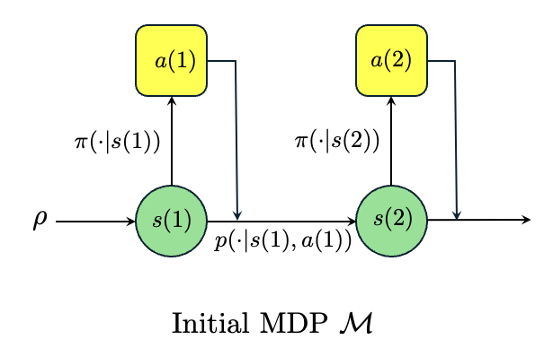
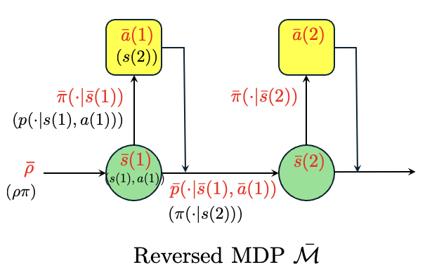
Figure 1: From the initial MDP (left) to the reversed MDP (right): In the reversed MDP, variables are shown in red; their initial MDP counterparts are shown in black.

For the reversed MDP, the discounted state-visitation distribution starting at $\bar{s}\in\bar{\mathcal{S}}$ is defined as:

$$\forall\bar{s}^{\prime}\in\bar{\mathcal{S}},\,d^{\bar{\pi}}_{\bar{p},\bar{s}}(\bar{s}^{\prime}):=(1-{\gamma})\mathbb{E}^{\pi}_{p}[\sum_{t=0}^{\infty}{\gamma}^{t}\mathbbm{1}\{\bar{s}(t)=\bar{s}^{\prime}\}\mid\bar{s}(0)=\bar{s}],$$

which is equal to $d^{\pi}_{p,s,a}(s^{\prime},a^{\prime})$ when $\bar{s}=(s,a)$ and $\bar{s}^{\prime}=(s^{\prime},a^{\prime})$. For any $\boldsymbol{\mu}\in\Delta(\bar{{\cal S}})$, we define $\bar{d}^{\pi}_{p,\boldsymbol{\mu}}(\bar{s}^{\prime}):=\sum_{\bar{s}\in\bar{\mathcal{S}}}\mu_{\bar{s}}\bar{d}^{\pi}_{p,\bar{s}}(\bar{s}^{\prime})$. The state and state-action value functions of $\bar{\cal M}$ are defined as: for all $(\bar{s},\bar{a})$:

$$\bar{V}^{\bar{\pi}}_{\bar{p}}(\bar{s}):=\mathbb{E}^{\pi}_{p}[\sum_{t=0}^{\infty}\gamma^{t}\bar{r}(\bar{s}(t),\bar{a}(t))|\bar{s}(0)=\bar{s}],$$ (7)

$$\bar{Q}^{\bar{\pi}}_{\bar{p}}(\bar{s},\bar{a}):=\mathbb{E}^{\pi}_{p}[\sum_{t=0}^{\infty}\gamma^{t}\bar{r}(\bar{s}(t),\bar{a}(t))|(\bar{s}(0),\bar{a}(0))=(\bar{s},\bar{a})].$$ (8)

For any $\boldsymbol{\mu}\in\Delta(\bar{{\cal S}})$, we define $\bar{V}^{\pi}_{p}(\boldsymbol{\mu}):=\sum_{\bar{s}\in\bar{\mathcal{S}}}\mu_{\bar{s}}\bar{V}^{\pi}_{p}(\bar{s})$. Observe that $\bar{V}^{\bar{\pi}}_{\bar{p}}(\bar{s})=Q^{\pi}_{p}(s,a)$ if $\bar{s}=(s,a)$, and $\bar{Q}^{\bar{\pi}}_{\bar{p}}(\bar{s},\bar{a})=r(s,a)+\gamma V^{\pi}_{p}(s^{\prime})$ if $(\bar{s},\bar{a})=(s,a,s^{\prime})$. We simply deduce that for each $s\in\mathcal{S}$, $V^{\pi}_{p}(s)=\sum_{a\in\mathcal{A}}\pi(a|s)\bar{V}^{\bar{\pi}}_{\bar{p}}(s,a)$, and $V^{\pi}_{p}(\boldsymbol{\rho})=\sum_{s\in\mathcal{S}}\sum_{a\in\mathcal{A}}\rho_{s}\pi(a|s)\bar{V}^{\bar{\pi}}_{\bar{p}}(s,a)=\bar{V}^{\bar{\pi}}_{\bar{p}}(\bar{\rho})$. Thus, optimizing transition kernel $q$ in (NO-$\sigma,\boldsymbol{\omega},p$) is equivalent to optimizing the policy against in the reversed MDP. More precisely, (NO-$\sigma,\boldsymbol{\omega},p$) is equivalent to:

$$\min_{\bar{\pi}\in{\cal P}}\bar{V}^{\bar{\pi}}_{\bar{p}}(\bar{\boldsymbol{\rho}})V^{\pi}_{p}(\boldsymbol{\rho}) \quad\text{s.t. }\sum_{s,a}\omega_{sa}\textnormal{KL}_{sa}(p,\bar{\pi})\leq\sigma.$$ (9)

Reformulating (NO-$\sigma,\boldsymbol{\omega},p$) as a policy optimization problem in the reversed MDP offers a key advantage: it allows us to leverage recent advances in the convergence analysis of policy gradient methods. In the next subsection, we build on this reformulation to analyze the resulting optimization algorithm.

6.3 Projected policy gradient

We apply policy gradient methods to solve (9). This problem is equivalent to (NO-$\sigma,\boldsymbol{\omega},p$) and consists in optimizing the policy of the reversed MDP. This policy corresponds to the transition kernel in the initial MDP. Before we present our algorithm, we provide preliminary results that will help its analysis. These results are the equivalent for our reversed MDP of the performance difference lemma (Kakade and Langford,, 2002), the policy gradient theorem (Sutton et al.,, 1999), and the smoothness lemma (Agarwal et al.,, 2021) for regular MDPs. Since as shown above for the reversed MDP, $\bar{V}^{\bar{\pi}}_{\bar{p}}(\bar{s})=Q^{\pi}_{p}(s,a)$ and the objective function $\bar{V}^{\bar{\pi}}_{\bar{p}}(\bar{\rho})=V^{\pi}_{p}(\boldsymbol{\rho})$ can be expressed using $Q^{\pi}_{p}(s,a)$, these results will essentially describe how $Q^{\pi}_{p}(s,a)$ evolves w.r.t. $p$. We start with the performance difference lemma, which interestingly, for the reversed MDP, corresponds to the celebrated simulation lemma (Kearns and Singh,, 2002) (also see Lemma A.1 in Vemula et al., (2023)).

Lemma 2 (Simulation / performance difference lemma).

For any $p,\tilde{p}\in\mathcal{P}$ and $(s,a)\in\mathcal{S}\times\mathcal{A}$,

$$Q^{\pi}_{p}(s,a)-Q^{\pi}_{\tilde{p}}(s,a)=\frac{\gamma}{1-\gamma}\sum_{s^{\prime}\in\mathcal{S},a^{\prime}\in\mathcal{A}}d^{\pi}_{p,s,a}(s^{\prime},a^{\prime})\sum_{s^{\prime\prime}\in\mathcal{S}}V^{\pi}_{\tilde{p}}(s^{\prime\prime})\left(p(s^{\prime\prime}\mid s^{\prime},a^{\prime})-\tilde{p}(s^{\prime\prime}\mid s^{\prime},a^{\prime})\right).$$

Lemma 2 is proved in Appendix D.4 for completeness. It directly implies that $Q^{\pi}_{p}(s,a)$ is continuous in $p$, a property that is used in the proof of Proposition 2.

Lemma 3 (Policy gradient).

For each $s,s^{\prime},s^{\prime\prime}\in\mathcal{S},\,a,a^{\prime}\in\mathcal{A}$, we have

$$\frac{\partial Q^{\pi}_{p}(s,a)}{\partial p(s^{\prime\prime}\mid s^{\prime},a^{\prime})} =\frac{1}{(1-\gamma)}d^{\pi}_{p,s,a}(s^{\prime},a^{\prime})\left(r(s^{\prime},a^{\prime})+\gamma V^{\pi}_{p}(s^{\prime\prime})\right),$$ (10)

$$\frac{\partial V^{\pi}_{p}(\boldsymbol{\rho})}{\partial p(s^{\prime}\mid s,a)} =\frac{1}{(1-\gamma)}d_{p,\boldsymbol{\rho}}^{\pi}(s,a)\left(r(s,a)+\gamma V^{\pi}_{p}(s^{\prime})\right).$$ (11)

The proof of this lemma is presented in Appendix D.5. It provides an explicit expression of the gradient $\nabla_{\bar{\pi}}\bar{V}^{\bar{\pi}}_{\bar{p}}(\bar{\boldsymbol{\rho}})$ used in our policy gradient algorithm. The final result concerns the smoothness of the gradient, and it can be established using tools from the theory of the policy gradient (Agarwal et al.,, 2021). It will be useful when assessing the convergence rate of our algorithm. Refer to Appendix D.6 for a proof.

Lemma 4 (Smoothness).

For any $p,\tilde{p}\in\mathcal{P}$ and $(s,a)\in\mathcal{S}\times\mathcal{A}$,

$$\left\|\nabla_{p}Q^{\pi}_{p}(s,a)-\nabla_{p}Q^{\pi}_{\tilde{p}}(s,a)\right\|_{2}\leq\frac{2\gamma\left|{\cal S}\right|}{(1-\gamma)^{3}}\left\|p-\tilde{p}\right\|_{2}.$$

Algorithm 2 Projected Policy Gradient

1:Input: $(p,\zeta,\sigma,\boldsymbol{\omega})$

2:Initialization:

3:Define $\bar{\mathcal{S}},\bar{\mathcal{A}},\bar{s},\bar{a},\bar{r},\bar{p}$, and $\bar{V}^{\bar{\pi}}_{\bar{p}}(\bar{\boldsymbol{\rho}})$ as in Section 6.2.

4:$M\leftarrow\lceil\left\|1/\bar{\boldsymbol{\rho}}\right\|_{\infty}^{2}(128\gamma|\bar{\mathcal{S}}||\bar{\mathcal{A}}|)/((1-\gamma)^{5}\zeta)\rceil$, $L\leftarrow 2{\gamma}\left|{\bar{\mathcal{A}}}\right|/(1-\gamma)^{3}|V^{\pi}_{p}(\boldsymbol{\rho})|$

5:$\bar{\pi}^{(0)}\leftarrow\text{Unif}(\bar{\mathcal{A}})$

6:for $k=0,1,\ldots,M-1$ do

7:  $\bar{\pi}^{(k+1)}\leftarrow\textnormal{\bf proj}_{\bar{\Pi}_{\sigma}^{p}}\left(\bar{\pi}^{(k)}-\frac{V_{\hat{p}}^{\pi}(\boldsymbol{\rho})}{L}\nabla_{\bar{\pi}}\bar{V}^{\bar{\pi}^{(k)}}_{\bar{p}}(\bar{\boldsymbol{\rho}})\right)$

8:end for

9:Output: $V_{p}^{\pi}(\boldsymbol{\rho})\bar{V}^{\bar{\pi}^{(M)}}_{\bar{p}}(\bar{\boldsymbol{\rho}})$

We are ready to present the policy gradient algorithm used to solve (9). In this problem, the constraint set $\Pi_{\sigma}^{p}:=\{\bar{\pi}\in\mathcal{P}:\sum_{s,a}\omega_{sa}\textnormal{KL}_{sa}(p,\bar{\pi})\leq\sigma\}$ is closed and convex. The algorithm, whose pseudo-code is presented in Algorithm 2, is hence a projected policy gradient algorithm, where in each iteration we make sure that the constraint is satisfied by projecting on $\Pi_{\sigma}^{p}$. Specifically, the policy updates of the algorithm are:

$$\bar{\pi}^{(k+1)}=\textnormal{\bf proj}_{\Pi_{\sigma}^{p}}\left(\bar{\pi}^{(k)}-\frac{V^{\pi}_{p}(\boldsymbol{\rho})}{L}\nabla_{\bar{\pi}}\bar{V}^{\bar{\pi}^{(k)}}_{\bar{p}}(\bar{\boldsymbol{\rho}})\right),$$ (12)

where $\textnormal{\bf proj}_{\Pi_{\sigma}^{p}}(x)$ denotes the projection of $x$ onto $\Pi_{\sigma}^{p}$ in the Euclidean norm and $L=\frac{2{\gamma}\left|{\bar{\mathcal{A}}}\right|}{(1-\gamma)^{3}|V^{\pi}_{p}(\boldsymbol{\rho})|}$. Observe that the value of (9) is $u_{\textnormal{NO}}(\sigma,\boldsymbol{\omega},p)$. The following theorem provides a finite time analysis of the projected gradient algorithm.

Theorem 3.

Under Assumption 1, 2, the projected policy gradient method (12) satisfies, for all $k\geq 1$, $\bar{V}^{\bar{\pi}^{(k)}}_{\bar{p}}(\bar{\boldsymbol{\rho}})V^{\pi}_{p}(\boldsymbol{\rho})-u_{\textnormal{NO}}(\sigma,\boldsymbol{\omega},p)$ is upper bounded by

$$\max\Bigg{\{}\frac{128\gamma|\bar{\mathcal{S}}||\bar{\mathcal{A}}|}{(1-\gamma)^{5}k}\left\|\frac{1}{\bar{\boldsymbol{\rho}}}\right\|_{\infty}^{2},\Big{(}\frac{1}{\sqrt{2}}\Big{)}^{k}\big{(}\bar{V}^{\bar{\pi}^{(0)}}_{\bar{p}}(\bar{\boldsymbol{\rho}})V^{\pi}_{p}(\boldsymbol{\rho})-u_{\textnormal{NO}}(\sigma,\boldsymbol{\omega},p)\big{)}\Bigg{\}}.$$

The proof of Theorem 3 is provided in Appendix D. This theorem motivates the design of Algorithm 2, which aims to approximate $u_{\textnormal{NO}}(\sigma,\boldsymbol{\omega},p)$ to within a specified accuracy level $\zeta$.

Finally, we note that when used in our policy testing algorithm (Algorithm 1), the unknown transition kernel $p$ in the input of Algorithm 2 is replaced by its empirical estimator $\hat{p}_{t}$, $\zeta$ is replaced by $\zeta_{t}$, $\boldsymbol{\omega}$ by $\hat{\boldsymbol{\omega}}(t)$, and $\sigma$ by the threshold $\beta(t,\delta)/t$.

7 Experiments

In this section, we test the proposed method in several scenarios. As a comparative method, we consider the KLB-TS algorithm proposed by Al Marjani and Proutiere, (2021). Unlike the setting of this paper, their approach aims to identify the best policy from among multiple candidate policies. To adapt their method to our setting, we prepared two policies: one identical to $\pi$ and another policy $\pi^{\prime}$ such that $V^{\pi^{\prime}}_{p}(\boldsymbol{\rho})=0$. We enforce uniform sampling for the sampling rule. The stopping rule of KLB-TS is based on an upper bound derived from a convexification of the original minimax optimization problem. Notably, this stopping rule does not explicitly utilize the fact that $V^{\pi^{\prime}}_{p}(\boldsymbol{\rho})=0$.

We conduct experiments using three MDP settings: $|\mathcal{S}|=|\mathcal{A}|=2$, $|\mathcal{S}|=|\mathcal{A}|=3$, and $|\mathcal{S}|=|\mathcal{A}|=5$. In all cases, the discount factor is set to $\gamma=0.9$ and the initial state distribution is uniform over all states. The reward function $r(s,a)$, the transition kernel $p(\cdot\mid s,a)$, and the policy $\pi$ are specified in Table 1, Table 2, and Table 3 in Appendix I for the respective settings. For each setting, we vary $\delta$ from $10^{-15}$ to $10^{-2}$. The results for $|\mathcal{S}|=|\mathcal{A}|=2$ are shown in the left panel of Figure 2, those for $|\mathcal{S}|=|\mathcal{A}|=3$ in the middle panel, and those for $|\mathcal{S}|=|\mathcal{A}|=5$ in the right panel. In all three cases, PTST outperforms KLB-TS for all values of $\delta$. For further details, please refer to Appendix I.

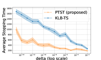
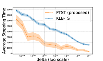
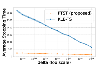
Figure 2: Comparison of average stopping times and delta for the proposed algorithm and KLB-TS. The left, center, and right panels correspond to $|\mathcal{S}|=|\mathcal{A}|=2,3,5$, respectively. Results are averaged over 30 instances. Error bars indicate the standard error of the mean.

8 Conclusion

In this paper, we formulated the policy testing problem in MDPs and characterized its instance-specific complexity. To the best of our knowledge, this is the first instance-specific optimal and computationally tractable algorithm for pure exploration in MDPs. The key components of our approach include a novel transformation of a non-convex problem and the use of policy gradients in the reversed MDP. Although our work specifically focuses on policy testing, we anticipate that our method can be extended to other pure exploration tasks, such as policy evaluation. This potential is discussed in Appendix C.2, where we outline the corresponding assumptions and minimization problems. Currently, our results are limited to the static sampling setting; extending them to adaptive sampling is an interesting direction for future work. Our findings could serve as a foundation for developing more efficient algorithms for pure exploration in MDPs.

Appendix A Further discussion on related works

Comparison with Thresholding Bandits.

When compared with the bandit literature, the policy testing problem can be regarded as a generalization of the thresholding bandit problem (Chen and Li,, 2015; Locatelli et al.,, 2016; Degenne and Koolen,, 2019; Wang et al.,, 2021), where the goal is to adaptively sample each arm and identify those whose mean reward exceeds a given threshold; our work generalizes this concept to the value function setting in MDPs. Similar settings using known thresholds in MABs have also led to other important variants, such as the good arm identification (Kano et al.,, 2019) and bad arm existence checking problems (Tabata et al.,, 2020). Such a setting has applications in scenarios with practical constraints on the horizon, such as in timely recommendations (Kano et al.,, 2019). It can also be viewed as an application of the concept of a satisficing objective (Russo and Van Roy,, 2022; Reverdy et al.,, 2016).

Analysis of Policy Gradient Methods.

Our analysis of the projected policy gradient method (Section 6.3) is partly based on recent advances in the analysis of convergence rates for policy gradient methods (Xiao,, 2022; Agarwal et al.,, 2021). While studies on the convergence rate of policy gradients with constraints exist (Ding et al.,, 2023; Montenegro et al.,, 2024), most focus on linear constraints on the state visitation distribution. In contrast, our results derive convergence rates under (convex but) nonlinear constraints, and provide rigorous sensitivity analysis of solutions with respect to these constraints (see Sections 5 and F), which is of independent technical interest.

Policy Evaluation.

Furthermore, our technique suggests that the instance-specific optimality is likely to be achievable for policy evaluation problems, including off-policy evaluation (Uehara et al.,, 2022) and more generally (Russo and Pacchiano,, 2025). We discuss the possibility of extending our results to policy evaluation in Section C.2.

Appendix B Instance-specific sample complexity lower bound–Proof of Theorem 1

Proof of Theorem 1.

Let $q\in\textnormal{Alt}(p)$, which is a nonempty set thanks to Assumption 1. Let $\mathbb{P}_{p}$ and $\mathbb{P}_{q}$ denote the probability measure generated by $p$ and $q$ respectively. According to property (i) of the $\delta$-PC algorithm definition, the stopping time $\tau$ is almost surely finite. Using Lemma 1 in Al Marjani and Proutiere, (2021) and the classical data processing inequality (see e.g. Lemma 1 in Kaufmann et al., (2016)), we derive that for any ${\cal F}_{\tau}$-measurable event $E$,

$$\sum_{s,a}\mathbb{E}_{p}[N_{sa}(\tau)]\textnormal{KL}_{sa}(p,q)\geq\textnormal{kl}(\mathbb{P}_{p}[E],\mathbb{P}_{q}[E]),$$ (13)

where $\textnormal{kl}(a,b)$ denotes the Kullback-Leibler (KL) divergence between two Bernoulli distributions with means $a$ and $b$. With choice $E=\{\hat{\imath}=\textnormal{Ans}(p)\}$, the definition of $\delta$ -PC algorithm (Definition 1) and the assumption that $q\in\textnormal{Alt}(p)$ yield that $\mathbb{P}_{p}[E]\geq 1-\delta$ and $\mathbb{P}_{q}[E]\leq\delta$. After applying the monotonicity of KL divergence, we obtain $\textnormal{kl}(\mathbb{P}_{p}[E],\mathbb{P}_{q}[E])\geq\textnormal{kl}(\delta,1-\delta)$. As (13) holds for any $q\in\textnormal{Alt}(p)$,

$$\textnormal{kl}(\delta,1-\delta) \leq\inf_{q\in\textnormal{Alt}(p)}\mathbb{E}_{p}[\tau]\sum_{s,a}\frac{\mathbb{E}_{p}[N_{sa}(\tau)]}{\mathbb{E}_{p}[\tau]}\textnormal{KL}_{sa}(p,q)$$

$$\leq\mathbb{E}_{p}[\tau]\left(\inf_{q\in\textnormal{Alt}(p)}\sum_{s,a}\omega_{sa}\textnormal{KL}_{sa}(p,q)+o(1)\right).$$ (14)

As $\forall\delta\in[0,1],\textnormal{kl}(\delta,1-\delta)\geq\log(2.4/\delta)\geq\log(1/\delta)$ and $\inf_{q\in\textnormal{Alt}(p)}\sum_{s,a}\omega_{sa}\textnormal{KL}_{sa}(p,q)>0$ by Proposition 1, the proof is completed by rearranging the inequality (B) and driving $\delta\to 0$. ∎

Appendix C Dual interpretation of the non-convex problems–Proof of Proposition 2

Here, the optimization problems (6.1) and (NO-$\sigma,\boldsymbol{\omega},p$) are abstracted as the following two optimization problems, respectively.

$$\inf_{x\in{\cal X}}h(x)\quad\text{s.t. }g(x)<u, u$$ (NC-)

and

$$\min_{x\in{\cal X}}g(x)\quad\text{s.t. }h(x)\leq\sigma, \sigma$$ (NO-)

where $h,g:{\cal X}\to\mathbb{R}\cup\{\infty\}$, ${\cal X}\subset\mathbb{R}^{d}$ is a nonempty set, $d\in\mathbb{N}$, and $u,\sigma\in\mathbb{R}$. Let $\sigma_{\textnormal{NC}}(u)$ and $u_{\textnormal{NO}}(\sigma)$ denote the value of (NC-$u$) and that of (NO-$\sigma$), respectively. As one can see, in Section 6.1, we make the substitutions $\mathcal{X}=\mathcal{P}$, $x=q$, $h(q)=\sum_{sa}\omega_{sa}\textnormal{KL}_{sa}(p,q)$, and $g(q)=V^{\pi}_{p}(\boldsymbol{\rho})V^{\pi}_{q}(\boldsymbol{\rho})$. As stated in Proposition 3, the desired bijection holds under the mild assumptions in Assumption 3. In Appendix C.1, we verify that these assumptions hold for the aforementioned substitution.

Assumption 3.

The following conditions hold.

1. $\exists\underline{x}\in\mathcal{X}$ such that $h(\underline{x})\leq 0$

2. $\min_{x\in\mathcal{X}}g(x)<0$.

3. All local minimums of $g$ ($h$ resp.) in $\mathcal{X}$ are global minimums of $g$ ($h$ resp.).

4. $h,g$ are continuous mappings.

The following proposition shows that, under Assumption 3, there exists a bijection between problems NC-$u$ and NO-$\sigma$.

Proposition 3.

Under Assumption 3, we have

$$\hbox{for all }\sigma\geq 0\hbox{ such that }u_{\textnormal{NO}}(\sigma)>\min_{x\in\mathcal{X}}g(x), \quad\sigma_{\textnormal{NC}}(u_{\textnormal{NO}}(\sigma))=\sigma,$$ (15)

$$\hbox{for all }u\in(\min_{x\in\mathcal{X}}g(x),u_{\textnormal{NO}}(0)] \quad u_{\textnormal{NO}}(\sigma_{\textnormal{NC}}(u))=u.$$ (16)

In words, $\sigma_{\textnormal{NC}}(u)$ and $u_{\textnormal{NO}}(\sigma)$ are one-to-one mappings as decreasing functions, and knowing the value of $u_{\textnormal{NO}}(\sigma)$ would be equivalent to knowing the value of $\sigma_{\textnormal{NC}}(u)$.

Proof of Proposition 3.

We first show (15). Let $\sigma\geq 0$ and $u=u_{\textnormal{NO}}(\sigma)>\min_{x\in\mathcal{X}}g(x)$. By Lemma 5 and Lemma 6, we get $\sigma_{\textnormal{NC}}(u)\leq\sigma$ and $\sigma_{\textnormal{NC}}(u)\geq\sigma$ respectively, which directly yield (15).
For proving (16), we consider $u\in(\min_{x\in\mathcal{X}}g(x),u_{\textnormal{NO}}(0)]$. Using intermediate value theorem and the continuity of $u_{\textnormal{NO}}(\cdot)$ proved in Lemma 20 given in Appendix G.3, we deduce that there is $\sigma\in[0,\infty)$ such that $u_{\textnormal{NO}}(\sigma)=u$. As a consequence,

$$u_{\textnormal{NO}}(\sigma_{\textnormal{NC}}(u))=u_{\textnormal{NO}}(\sigma_{\textnormal{NC}}(u_{\textnormal{NO}}(\sigma)))=u_{\textnormal{NO}}(\sigma)=u,$$

where the second equation is the application of (15).

∎

Lemma 5.

Under Assumption 3, whenever $\sigma\geq 0,u\in(\min_{x\in\mathcal{X}}g(x),\infty)$, and $u_{\textnormal{NO}}(\sigma)\leq u$, then $\sigma_{\textnormal{NC}}(u)\leq\sigma$ holds.

Proof of Lemma 5.

As $u_{\textnormal{NO}}(\sigma)\leq u$, $\exists x^{\prime}\in\mathcal{X}$, such that $h(x^{\prime})\leq\sigma$, and $g(x^{\prime})\leq u$. If $g(x^{\prime})<u$ (case i), then $x^{\prime}$ is a feasible point for (NC-$u$), and therefore $\sigma_{\textnormal{NC}}(u)\leq h(x^{\prime})\leq\sigma$. We next consider the case where $g(x^{\prime})=u$ (case ii).
Since $g(x^{\prime})=u>\min_{x\in\mathcal{X}}g(x)$, $x^{\prime}$ is not a global minimum of $g$ in $\mathcal{X}$. Hence, by Assumption 3-(c), we deduce that $x^{\prime}$ is not a local minimum either. Thus, there is a sequence of $\{x_{n}\}_{n=1}^{\infty}$ such that $x_{n}\xrightarrow{n\to\infty}x^{\prime}$ and $g(x_{n})<u,\,\forall n$. As a consequence of Assumption 3-(d), $\lim_{n\to\infty}h(x_{n})=h(x^{\prime})\leq\sigma$, which yields $\sigma_{\textnormal{NC}}(u)\leq\sigma$. ∎

Lemma 6.

Whenever $\sigma\geq 0,u\in\mathbb{R}$ and $u_{\textnormal{NO}}(\sigma)\geq u$, $\sigma_{\textnormal{NC}}(u)\geq\sigma$ holds.

Proof of Lemma 6.

Suppose in contrast, $\sigma_{\textnormal{NC}}(u)<\sigma$. There exist $x\in{\cal X}$ such that $g(x)<u,\,h(x)<\sigma$. Hence $u_{\textnormal{NO}}(\sigma)<u$, which contradicts that $u_{\textnormal{NO}}(x)\geq u$. ∎

C.1 Proof of Proposition 2

Proof of Proposition 2.

Thanks to Proposition 3, the proof is completed by verifying that the following substitutions satisfy Assumption 3 when $p\in\mathcal{P}_{\textnormal{Test}}$.

$$\mathcal{X}={\cal P}, x=q,$$

$$h(q)=\sum_{s,a}\omega_{sa}\textnormal{KL}_{sa}(p,q), g(q)=V_{q}^{\pi}(\boldsymbol{\rho})V_{p}^{\pi}(\boldsymbol{\rho}).$$

(a) Let $\underline{x}=p$, one has that $h(\underline{x})=\sum_{sa}w_{sa}\textnormal{KL}_{sa}(p,p)=0$.
(b) Due to Assumption 1 and inequalities (1), there exists $q\in\mathcal{P}$ such that $\text{sign}(V^{\pi}_{q}(\boldsymbol{\rho}))\neq\text{sign}(V^{\pi}_{p}(\boldsymbol{\rho}))$, we have $\min_{x\in\mathcal{X}}g(x)\leq V^{\pi}_{q}(\boldsymbol{\rho})V^{\pi}_{p}(\boldsymbol{\rho})<0$.
(c) The local minimum of $h$ is the global minimum since $h$ is a convex function. As for $g$, we reverse the policy and transition kernel as in Section 6.2. Since the reversed MDP is still a tabular MDP, Theorem 1 in Bhandari and Russo, (2024) has verified that all the stationary points for the value function on the policy space are global optima. As a consequence, the local minimum of $g$ is the global minimum.
(d) It is clear that $h$ is a continuous function. The continuity of $g$ directly follows from the simulation lemma (Lemma 2).
∎

C.2 On the policy evaluation

Policy evaluation is the task where we aim to approximate the value of a given policy up to a predetermined constant $\varepsilon$ with a certain confidence. Specifically, if $\hat{v}$ denotes the approximation of $V^{\pi}_{p}(\boldsymbol{\rho})$, the goal is to minimize the number of samples $\mathbb{E}_{p}[\tau]$ while satisfying $\mathbb{P}_{p}[\left|\hat{v}-V^{\pi}_{p}(\boldsymbol{\rho})\right|>\varepsilon]<\delta$. Similar to Assumption 1 considered for the policy testing, we present Assumption 4 for policy evaluation. Notice that if Assumption 4 does not hold, returning $\hat{v}$ as an arbitrary value between $r^{\pi}(\boldsymbol{\rho})+\min_{s}\frac{\gamma}{1-\gamma}r^{\pi}(s)$ and $r^{\pi}(\boldsymbol{\rho})+\max_{s}\frac{\gamma}{1-\gamma}r^{\pi}(s)$ satisfies that $\left|\hat{v}-V^{\pi}_{p}(\boldsymbol{\rho})\right|\leq\varepsilon$.

Assumption 4.

$\rho_{s}>0$ for all $s\in{\cal S}$. $r$ and $\boldsymbol{\rho}$ satisfy:

$$\max_{s}\frac{\gamma}{1-\gamma}r^{\pi}(s)-\min_{s}\frac{\gamma}{1-\gamma}r^{\pi}(s)>\varepsilon.$$

As discussed in Section 5 and 6.1, solving the stopping condition boils down to identify whether the minimal value of the following two optimization problems is larger than $\beta(t,\delta)/t$.

$$\inf_{q}\sum_{s,a}\omega_{sa}\textnormal{KL}_{sa}(p,q) \quad\text{s.t. }V^{\pi}_{q}(\boldsymbol{\rho})-V^{\pi}_{p}(\boldsymbol{\rho})+\varepsilon<0,$$ (17)

and

$$\inf_{q}\sum_{s,a}\omega_{sa}\textnormal{KL}_{sa}(p,q) \quad\text{s.t. }V^{\pi}_{p}(\boldsymbol{\rho})-V^{\pi}_{q}(\boldsymbol{\rho})+\varepsilon<0.$$ (18)

Under Assumption 4, either $\{q\in\mathcal{P}:V^{\pi}_{q}(\boldsymbol{\rho})-V^{\pi}_{p}(\boldsymbol{\rho})+\varepsilon<0\}$ or $\{q\in\mathcal{P}:V^{\pi}_{p}(\boldsymbol{\rho})-V^{\pi}_{q}(\boldsymbol{\rho})+\varepsilon<0\}$ will be nonempty. For simplicity, we restrict our attention to solving (18) and assume $\{q\in\mathcal{P}:V^{\pi}_{p}(\boldsymbol{\rho})-V^{\pi}_{q}(\boldsymbol{\rho})+\varepsilon<0\}\neq\emptyset$. In the following, we prove Assumption 3 holds with the corresponding substitution in Lemma 7, then one can implement a projected policy gradient method to approximate the value of its dual problem, as described in Section 6.3.

$$\min_{q}V^{\pi}_{p}(\boldsymbol{\rho})-V^{\pi}_{q}(\boldsymbol{\rho})+\varepsilon \quad\hbox{s.t.}\sum_{sa}\omega_{sa}\textnormal{KL}_{sa}(p,q)\leq\frac{\beta(t,\delta)}{t}.$$ (19)

Lemma 7.

When $\{q\in\mathcal{P}:V^{\pi}_{p}(\boldsymbol{\rho})-V^{\pi}_{q}(\boldsymbol{\rho})+\varepsilon<0\}\neq\emptyset$, Assumption 3 holds with the following substitution.

$$\mathcal{X}={\cal P}, x=q,$$

$$h(q)=\sum_{s,a}\omega_{sa}\textnormal{KL}_{sa}(p,q), g(q)=V^{\pi}_{p}(\boldsymbol{\rho})-V^{\pi}_{q}(\boldsymbol{\rho})+\varepsilon.$$

Proof.

(a) Let $\underline{x}=p$, one has that $h(\underline{x})=\sum_{sa}w_{sa}\textnormal{KL}_{sa}(p,p)=0$.
(b) is a direct consequence of the assumption that $\{q\in\mathcal{P}:V^{\pi}_{p}(\boldsymbol{\rho})-V^{\pi}_{q}(\boldsymbol{\rho})+\varepsilon<0\}\neq\emptyset$.
(c) and (d) hold as the proof in Proposition 2. ∎

Appendix D Convergence analysis of constrained policy gradient–Proof of Theorem 3

For notational simplicity and clarity in the following description, we assume $V^{\pi}_{p}(\boldsymbol{\rho})=1$ and omit the $\bar{\square}$ notation. Moreover, we write $\Pi_{\sigma}$ instead of $\Pi_{\sigma}^{p}$ for brevity.

Proof of Theorem 3.

Consider the minimization problem of a smooth function as follows.

$$\min_{x\in Q}f(x),$$

where $Q$ is a closed, convex subset of $\mathbb{R}^{n}$ and $f(x)$ is $L$-smooth, i.e., there exists a constant $L>0$ such that

$$\|\nabla_{x}f(x)-\nabla_{x}f(y)\|_{2}\leq L\|x-y\|_{2},\qquad\forall x,y\in Q.$$

We consider the projected gradient descent algorithm for this optimization problem:

$$x^{(k+1)}=\textnormal{\bf proj}_{Q}\left(x^{(k)}-\frac{1}{L}\nabla_{x}f(x^{(k)})\right).$$ (20)

We first employ the following (weak) gradient-mapping condition introduced in Xiao, (2022).

Definition 2 (gradient-mapping domination Xiao, (2022)).

Consider the $L$-smooth objective function $f(x)$ and let $Q$ be a compact convex set. $f(x)$ satisfies the gradient-mapping dominance condition if for some constant $\omega>0$:

$$\|G_{L}(x)\|_{2}\geq\sqrt{2\omega}\left(f(T_{L}(x)-f^{\star})\right),\qquad\forall x\in Q,$$

where $f^{\star}=\min_{x\in Q}f(x)$, and $T_{L}(x),G_{L}(x)$ are defined as

$$T_{L}(x):=\textnormal{\bf proj}_{Q}\left(x-\frac{1}{L}\nabla_{x}f(x)\right),\qquad G_{L}(x):=L(x-T_{L}(x)).$$

Under the assumption that gradient-mapping domination condition holds, the following (global) convergence rate is obtained.

Theorem 4 (Xiao, (2022)).

Consider the minimization problem of an $L$-smooth function $f(x)$ over a convex compact set $Q$. Denote $f^{\star}=\min_{x\in Q}f(x)$. Suppose that $f(x)$ satisfies the gradient-mapping domination condition (with constant $\omega>0$ as defined above). Then, the sequence $(x^{(k)})_{k\geq 0}$ generated by the projected gradient descent algorithm (20) satisfies, for all $k\geq 1$,

$$f(x^{(k)})-f^{\star}\leq\max\Bigg{\{}\frac{4L}{\omega k},\Big{(}\frac{\sqrt{2}}{2}\Big{)}^{k}(f(x^{(0)})-f^{\star})\Bigg{\}}.$$

We present the proof of Theorem 4 in Appendix D.1 for completeness.

We now present the convergence rate of the projected policy gradient method over the convex compact subset $\Pi_{c}$:

$$\pi^{(k+1)}=\textnormal{\bf proj}_{\Pi_{\sigma}}\left(\pi^{(k)}-\frac{1}{L}\nabla_{\pi}V^{\pi^{(k)}}_{p}(\boldsymbol{\rho})\right).$$ (21)

We now consider the convergence rate under the $L$-smoothness assumption of the value function:

Lemma 8.

Suppose that $V_{p}^{\pi}(\boldsymbol{\rho})$ satisfies $L$-smoothness with respect to $\pi$. Then, the constrained projected policy gradient method (21) satisfies, for all $k\geq 1$,

$$V^{\pi^{(k)}}_{p}(\boldsymbol{\rho})-V^{\sigma\star}_{p}(\boldsymbol{\rho})\leq\max\Bigg{\{}\frac{64L|\mathcal{S}|}{(1-\gamma)^{2}k}\left\|\frac{1}{\boldsymbol{\rho}}\right\|_{\infty}^{2},\Big{(}\frac{\sqrt{2}}{2}\Big{)}^{k}(V^{\pi^{(0)}}_{p}(\boldsymbol{\rho})-V_{p}^{\sigma\star}(\boldsymbol{\rho}))\Bigg{\}}.$$

The proof of Lemma 8 is presented in Appendix D.2.

In Lemma 54 in Agarwal et al., (2021), the authors show the smoothness of the value function, that is,

$$\left\|\nabla_{{\pi}}{V}^{{\pi}}_{{p}}(\boldsymbol{\rho})-\nabla_{{\pi}}V^{\tilde{{\pi}}}_{p}(\boldsymbol{\rho})\right\|_{2}\leq\frac{2{\gamma}\left|{\mathcal{A}}\right|}{(1-{\gamma})^{3}}\left\|{\pi}-\tilde{{\pi}}\right\|_{2},\qquad\forall\pi,\tilde{\pi}\in\Pi.$$

Therefore, ${V}^{{\pi}}_{{p}}(\boldsymbol{\rho})$ satisfies $L$-smoothness by taking

$$L=\frac{2{\gamma}\left|{\mathcal{A}}\right|}{(1-{\gamma})^{3}}.$$ (22)

Theorem 3 is an immediate consequence from Lemma 8 and (22).

∎

D.1 Proof of Theorem 4

Proof of Theorem 4.

We obtain, for any $x\in Q$,

$$f(x)-f(T_{L}(x)) \geq\frac{1}{2L}\|G_{L}(x)\|_{2}^{2}$$

$$\geq\frac{\omega}{L}(f(T_{L}(x))-f^{\star})^{2}.$$

where for the first inequality, we used Theorem 1 of Nesterov, (2013), and for the second inequality, the gradient-mapping domination condition is used. We obtain, for each $s\geq 0$,

$$f(x^{(s)})-f(x^{(s+1)})\geq\frac{\omega}{L}(f(x^{(s+1)})-f^{\star})^{2}.$$ (23)

Denote $\delta_{s}=f(x^{(s)})-f^{\star}$; note that $\delta_{s}\geq 0$. We obtain:

$$\qquad f(x^{(s)})-f(x^{(s+1)})=\delta_{s}-\delta_{s+1}\geq\frac{\omega}{L}\delta_{s+1}^{2}$$

$$\text{which is equivalent to }\frac{1}{\delta_{s+1}}-\frac{1}{\delta_{s}}\geq\frac{\omega}{L}\frac{\delta_{s+1}}{\delta_{s}}.$$

Summing up the inequality from $s=0$ to $s=k-1$, we obtain:

$$\frac{1}{\delta_{k}}-\frac{1}{\delta_{0}}\geq\frac{\omega}{L}\sum_{s=0}^{k-1}\frac{\delta_{s+1}}{\delta_{s}}.$$

Using a constant $r\in(0,1)$, we define $n(k,r)$ as the number of times the ratio $\delta_{s+1}/\delta_{s}$ is at least $r$ among the first $k$ iterations. Let $c\in(0,1)$ be a constant. Suppose $n(k,r)\geq ck$; then $\delta_{s+1}/\delta_{s}\geq r$ for at least $\lceil ck\rceil$ values of $s$ in $\{0,\dots,k-1\}$. In this case,

$$\frac{\omega}{L}rck\leq\frac{1}{\delta_{k}}-\frac{1}{\delta_{0}}\leq\frac{1}{\delta_{k}}.$$

Then, we derive that

$$\delta_{k}\leq\frac{L}{\omega rck}.$$

Otherwise, when $n(k,r)<ck$, it holds that $\delta_{s+1}/\delta_{s}<r$ at least $\lceil(1-c)k\rceil$ times. From the descent property (23), we further obtain $\delta_{s+1}\leq\delta_{s}\leq 1$ for each $s\in\{0,\ldots,k-1\}$. Therefore, we get

$$\delta_{k}=\frac{\delta_{k}}{\delta_{k-1}}\frac{\delta_{k-1}}{\delta_{k-2}}\cdots\frac{\delta_{1}}{\delta_{0}}\delta_{0}<\delta_{0}r^{(1-c)k}.$$

Therefore, by taking $c=r=1/2$, we obtain,

$$\delta_{k}\leq\max\left\{\frac{4L}{\omega k},\left(\frac{1}{\sqrt{2}}\right)^{k}\delta_{0}\right\}.$$

This concludes the proof. ∎

D.2 Proof of Lemma 8

Proof of Lemma 8.

Define

$$T_{L}(\pi):=\textnormal{\bf proj}_{\Pi_{\sigma}}\left(\pi-\frac{1}{L}\nabla_{\pi}V^{\pi}_{p}(\boldsymbol{\rho})\right),\qquad G_{L}(\pi):=L(\pi-T_{L}(\pi)).$$

The following gradient mapping domination condition for the projected policy gradient can be proved.

Lemma 9 (Weak gradient-mapping domination).

Let $\Pi_{\sigma}$ be a closed and convex subset of $\Pi$, $V^{\sigma\star}_{p}(\boldsymbol{\rho}):=\min_{\pi\in\Pi_{\sigma}}V^{\pi}_{p}(\boldsymbol{\rho})$, and $\pi^{\star}\in\operatorname*{arg\,min}_{\pi^{\prime}\in\Pi}V^{\pi^{\prime}}_{p}(\boldsymbol{\rho})$. Assume that $V_{p}^{\pi}(\boldsymbol{\rho})$ satisfies $L$-smoothness with respect to $\pi$, i.e., the following holds:

$$\|\nabla_{\pi}V_{p}^{\pi}(\boldsymbol{\rho})-\nabla_{\pi}V_{p}^{\pi^{\prime}}(\boldsymbol{\rho})\|_{2}\leq L\|\pi-\pi^{\prime}\|_{2},\qquad\forall\pi,\pi^{\prime}\in\Pi_{\sigma}.$$

Then, we have, for all $\pi\in\Pi_{\sigma}$,

$$V^{T_{L}(\pi)}_{p}(\boldsymbol{\rho})-V^{\sigma\star}_{p}(\boldsymbol{\rho})\leq\frac{2\sqrt{2|\mathcal{S}|}}{1-\gamma}\left\|\frac{1}{\boldsymbol{\rho}}\right\|_{\infty}\|G_{L}(\pi)\|_{2},$$

where

$$T_{L}(\pi):=\textnormal{\bf proj}_{\Pi_{\sigma}}\left(\pi-\frac{1}{L}\nabla_{\pi}V^{\pi}_{p}(\boldsymbol{\rho})\right),\qquad G_{L}(\pi):=L(\pi-T_{L}(\pi)).$$

The proof of Lemma 9 is presented in Appendix D.3.

From Lemma 9, for all $\pi\in\Pi_{\sigma}$,

$$V^{T_{L}(\pi)}_{p}(\boldsymbol{\rho})-V^{\sigma\star}_{p}(\boldsymbol{\rho})\leq\frac{2\sqrt{2|\mathcal{S}|}}{1-\gamma}\left\|\frac{1}{\boldsymbol{\rho}}\right\|_{\infty}\|G_{L}(\pi)\|_{2}.$$

Therefore, the gradient-mapping dominantion condition holds with

$$\omega=\frac{(1-\gamma)^{2}}{16|\mathcal{S}|\left\|\frac{1}{\boldsymbol{\rho}}\right\|_{\infty}^{2}}.$$

From Theorem 4, we obtain

$$V^{\pi^{(k)}}_{p}(\boldsymbol{\rho})-V^{\sigma\star}_{p}(\boldsymbol{\rho})\leq\max\Bigg{\{}\frac{64L|\mathcal{S}|}{(1-\gamma)^{2}k}\left\|\frac{1}{\boldsymbol{\rho}}\right\|_{\infty}^{2},\Big{(}\frac{\sqrt{2}}{2}\Big{)}^{k}(V^{\pi^{(0)}}_{p}(\boldsymbol{\rho})-V_{p}^{\sigma\star}(\boldsymbol{\rho}))\Bigg{\}}$$

This concludes the proof. ∎

D.3 Proof of Lemma 9

Proof of Lemma 9.

We apply Theorem 1 from Nesterov, (2013). By setting $Q=\Pi$ and $\Psi$ as the indicator function of $\Pi_{\sigma}$, we deduce that

$$\langle\nabla_{\pi}V_{p}^{\pi}(\boldsymbol{\rho}),T_{L}(\pi)-\pi^{\prime}\rangle\leq 2\|G_{L}(\pi)\|_{2}\|T_{L}(\pi)-\pi^{\prime}\|_{2},\qquad\forall\pi,\pi^{\prime}\in\Pi.$$

From $T_{L}(\pi)\in\Pi$, we obtain $\|T_{L}(\pi)-\pi^{\prime}\|\leq\sqrt{2|\mathcal{S}|}$. We further deduce that

$$\max_{\pi^{\prime}\in\Pi}\langle\nabla_{\pi}V_{p}^{\pi}(\boldsymbol{\rho}),T_{L}(\pi)-\pi^{\prime}\rangle\leq 2\sqrt{2|\mathcal{S}|}\|G_{L}(\pi)\|_{2}.$$

Let $V^{\star}_{p}(\boldsymbol{\rho})=\min_{\pi^{\prime}\in\Pi}V^{\pi^{\prime}}_{p}(\boldsymbol{\rho})$ and $\pi^{\star}\in\operatorname*{arg\,min}_{\pi^{\prime}\in\Pi}V^{\pi^{\prime}}_{p}(\boldsymbol{\rho})$. As $\Pi_{\sigma}\subseteq\Pi$, we obtain

$$V^{T_{L}(\pi)}_{p}(\boldsymbol{\rho})-V^{\sigma\star}_{p}(\boldsymbol{\rho})\leq V^{T_{L}(\pi)}_{p}(\boldsymbol{\rho})-V^{\star}_{p}(\boldsymbol{\rho}) \leq\frac{1}{1-\gamma}\left\|\frac{1}{\boldsymbol{\rho}}\right\|_{\infty}\max_{\pi^{\prime}\in\Pi}\langle\nabla_{\pi}V^{\pi}_{p}(\boldsymbol{\rho}),T_{L}(\pi)-\pi^{\prime}\rangle$$

$$\leq\frac{2\sqrt{2|\mathcal{S}|}}{1-\gamma}\left\|\frac{1}{\boldsymbol{\rho}}\right\|_{\infty}\|G_{L}(\pi)\|_{2},$$

where the second inequality follows from Lemma 10 below.

Lemma 10 (Variational gradient domination, Lemma 4 in Agarwal et al., (2021)).

Let $V^{\star}_{p}(\boldsymbol{\rho})=\min_{\pi^{\prime}\in\Pi}V^{\pi^{\prime}}_{p}(\boldsymbol{\rho})$ and $\pi^{\star}\in\operatorname*{arg\,min}_{\pi^{\prime}\in\Pi}V^{\pi^{\prime}}_{p}(\boldsymbol{\rho})$. We have, for any $\pi\in\Pi$,

$$V^{\pi}_{p}(\boldsymbol{\rho})-V^{\star}_{p}(\boldsymbol{\rho}) \leq\left\|\frac{d^{\pi^{\star}}_{p,\boldsymbol{\rho}}}{d^{\pi}_{p,\boldsymbol{\rho}}}\right\|_{\infty}\max_{\pi^{\prime}\in\Pi}\langle\nabla_{\pi}V^{\pi}_{p}(\boldsymbol{\rho}),\pi-\pi^{\prime}\rangle$$

$$\leq\frac{1}{1-\gamma}\left\|\frac{d^{\pi^{\star}}_{p,\boldsymbol{\rho}}}{\boldsymbol{\rho}}\right\|_{\infty}\max_{\pi^{\prime}\in\Pi}\langle\nabla_{\pi}V^{\pi}_{p}(\boldsymbol{\rho}),\pi-\pi^{\prime}\rangle$$

$$\leq\frac{1}{1-\gamma}\left\|\frac{1}{\boldsymbol{\rho}}\right\|_{\infty}\max_{\pi^{\prime}\in\Pi}\langle\nabla_{\pi}V^{\pi}_{p}(\boldsymbol{\rho}),\pi-\pi^{\prime}\rangle.$$

This concludes the proof. ∎

D.4 Proof of Lemma 2

Proof of Lemma 2.

Let $\bar{s}=(s,a)$, $\bar{p}$ is the transition kernel yielded by $\pi$, and $\bar{\pi}$ ($\tilde{\bar{\pi}}$ resp.) is the policy yielded by $p$ ($\tilde{p}$ resp.). Invoke the performance difference lemma, we have

$$\bar{V}^{\bar{\pi}}_{\bar{p}}(\bar{s})-\bar{V}^{\tilde{\bar{\pi}}}_{\bar{p}}(\bar{s})=\frac{1}{1-\gamma}\sum_{\bar{s}^{\prime}\in\bar{\mathcal{S}}}\bar{d}^{\bar{\pi}}_{\bar{p},\bar{s}}(\bar{s}^{\prime})\sum_{\bar{a}^{\prime\prime}\in\bar{\mathcal{A}}}\bar{Q}^{\tilde{\bar{\pi}}}_{\bar{p}}(\bar{s}^{\prime},\bar{a}^{\prime\prime})\left(\bar{\pi}(\bar{a}^{\prime\prime}\mid\bar{s}^{\prime})-\tilde{\bar{\pi}}(\bar{a}^{\prime\prime}\mid\bar{s}^{\prime})\right).$$ (24)

Observe that the L.H.S. of (24) is exactly $Q^{\pi}_{p}(s,a)-Q^{\pi}_{\tilde{p}}(s,a)$. Next denote $\bar{s}^{\prime}=(s^{\prime},a^{\prime})$ and $\bar{a}^{\prime\prime}=s^{\prime\prime}$, then the proof is completed by substituting the R.H.S of (24) with $\bar{d}^{\bar{\pi}}_{\bar{p},\bar{s}}(\bar{s}^{\prime})=d^{\pi}_{p,s,a}(s^{\prime},a^{\prime})$,

$$\sum_{\bar{a}^{\prime\prime}\in\bar{\mathcal{A}}}\bar{Q}^{\tilde{\bar{\pi}}}_{\bar{p}}(\bar{s}^{\prime},\bar{a}^{\prime\prime})\bar{\pi}(\bar{a}^{\prime\prime}\mid\bar{s}^{\prime}) =r(s^{\prime},a^{\prime})+\gamma\sum_{s^{\prime\prime}\in\mathcal{S}}p(s^{\prime\prime}\mid s^{\prime},a^{\prime})V^{\pi}_{\tilde{p}}(s^{\prime\prime}),$$

and

$$\sum_{\bar{a}^{\prime\prime}\in\bar{\mathcal{A}}}\bar{Q}^{\tilde{\bar{\pi}}}_{\bar{p}}(\bar{s}^{\prime},\bar{a}^{\prime\prime})\tilde{\bar{\pi}}(\bar{a}^{\prime\prime}\mid\bar{s}^{\prime}) =r(s^{\prime},a^{\prime})+\gamma\sum_{s^{\prime\prime}\in\mathcal{S}}\tilde{p}(s^{\prime\prime}\mid s^{\prime},a^{\prime})V^{\pi}_{\tilde{p}}(s^{\prime\prime}).$$

This concludes the proof. ∎

D.5 Proof of Lemma 3

Proof of Lemma 3.

Show (10). Let $\bar{s}=(s,a),\bar{s}^{\prime}=(s^{\prime},a^{\prime}),\bar{a}^{\prime\prime}=s^{\prime\prime}$. The policy gradient on $\bar{V}^{\bar{\pi}}_{p}(\bar{s})$, which equals to $Q^{\pi}_{p}(s,a)$, with respect to $\bar{\pi}(\bar{a}^{\prime\prime}\mid\bar{s}^{\prime})$, is

$$\frac{\partial\bar{V}^{\bar{\pi}}_{p}(\bar{s})}{\partial\bar{\pi}(\bar{a}^{\prime\prime}\mid\bar{s}^{\prime})}=\frac{1}{1-\gamma}\bar{d}^{\bar{\pi}}_{\bar{p},\bar{s}}(\bar{s}^{\prime})\bar{Q}^{\bar{\pi}}_{\bar{p}}(\bar{s}^{\prime},\bar{a}^{\prime\prime}).$$

The proof of (10) is completed as: $\bar{d}^{\bar{\pi}}_{\bar{p},\bar{s}}(\bar{s}^{\prime})=d^{\pi}_{p,s,a}(s^{\prime},a^{\prime})$, and

$$\bar{Q}^{\bar{\pi}}_{\bar{p}}(\bar{s}^{\prime},\bar{a}^{\prime\prime})=r(s^{\prime},a^{\prime})+\gamma V^{\pi}_{p}(s^{\prime\prime}).$$

Show (11). As $V^{\pi}_{p}(\boldsymbol{\rho})=\sum_{\tilde{s},\tilde{a}}\rho_{\tilde{s}}\pi(\tilde{a}\mid\tilde{s})Q^{\pi}_{p}(\tilde{s},\tilde{a})$. Using (10), one obtains

$$\frac{\partial V^{\pi}_{p}(\boldsymbol{\rho})}{\partial p(s^{\prime}\mid s,a)} =\sum_{\tilde{s},\tilde{a}}\rho_{\tilde{s}}\pi(\tilde{a}\mid\tilde{s})\frac{1}{1-\gamma}d_{p,\tilde{s},\tilde{a}}^{\pi}(s,a)\left(r(s,a)+\gamma V^{\pi}_{p}(s^{\prime})\right)$$

$$=\frac{1}{(1-\gamma)}d_{p,\boldsymbol{\rho}}^{\pi}(s,a)\left(r(s,a)+\gamma V^{\pi}_{p}(s^{\prime})\right).$$

∎

D.6 Proof of Lemma 4

Proof of Lemma 4.

Let $\bar{s}=(s,a)$, and $\bar{\pi}$ ($\tilde{\bar{\pi}}$ resp.) denotes the policy yielded by $p$ ($\tilde{p}$ resp.). Applying Lemma 54 in Agarwal et al., (2021) implies that

$$\left\|\nabla_{\bar{\pi}}\bar{V}^{\bar{\pi}}_{\bar{p}}(\bar{s})-\nabla_{\bar{\pi}}\bar{V}^{\tilde{\bar{\pi}}}_{\bar{p}}(\bar{s})\right\|_{2}\leq\frac{2\gamma\left|\bar{\mathcal{A}}\right|}{(1-\gamma)^{3}}\left\|\bar{\pi}-\tilde{\bar{\pi}}\right\|_{2}.$$

The lemma directly stems from the facts that

$$\nabla_{\bar{\pi}}\bar{V}^{\bar{\pi}}_{\bar{p}}(\bar{s})=\nabla_{p}Q^{\pi}_{p}(s,a),\nabla_{\bar{\pi}}\bar{V}^{\tilde{\bar{\pi}}}_{\bar{p}}(\bar{s})=\nabla_{p}Q^{\pi}_{\tilde{p}}(s,a),\text{ and }\bar{\mathcal{A}}=\mathcal{S}.$$

∎

Appendix E Upper bound on the sample complexity–Proof of Theorem 2

Convention. Throughout this section, for simplicity of presentation, we assume $\text{Ans}(p)=+$.

Proof of Theorem 2.

Show $\delta$-PC. Recall that Algorithm 1 stops in round $\tau$ only if $u_{\zeta_{\tau}}-\zeta_{\tau}>0$. Thanks to Theorem 3 and the number of iterations $M$ chosen in Algorithm 2, we have

$$u_{\textnormal{NO}}(\beta(\tau,\delta)/\tau,\hat{\boldsymbol{\omega}}(\tau),\hat{p}_{\tau})\geq u_{\zeta_{\tau}}-\zeta_{\tau}>0.$$ (25)

As Assumption 1 implies that $\min_{q}V^{\pi}_{q}(\boldsymbol{\rho})V^{\pi}_{\hat{p}_{\tau}}(\boldsymbol{\rho})<0$, inequality (25) yields that

$$u_{\textnormal{NO}}(\beta(\tau,\delta)/\tau,\hat{\boldsymbol{\omega}}(\tau),\hat{p}_{\tau})>\min_{q}V^{\pi}_{q}(\boldsymbol{\rho})V^{\pi}_{\hat{p}_{\tau}}(\boldsymbol{\rho}).$$ (26)

Observing that $\sigma_{\textnormal{NC}}(\cdot,\hat{\boldsymbol{\omega}}(\tau),\hat{p}_{\tau})$ is a decreasing function, (25) also yields that

$$\sigma_{\textnormal{NC}}(0,\hat{\boldsymbol{\omega}}(\tau),\hat{p}_{\tau})\geq\sigma_{\textnormal{NC}}(u_{\textnormal{NO}}(\beta(\tau,\delta)/\tau,\hat{\boldsymbol{\omega}}(\tau),\hat{p}_{\tau}),\hat{\boldsymbol{\omega}}(\tau),\hat{p}_{\tau})=\beta(\tau,\delta)/\tau,$$ (27)

where the last equality follows from Proposition 2 with $\sigma=\beta(\tau,\delta)/\tau\geq 0$ and condition (26). One can notice that (27) is equivalent to (6). Hence, if $\textnormal{Ans}(\hat{p}_{\tau})\neq\textnormal{Ans}(p)$ (in other words, if $p\in\textnormal{Alt}(\hat{p}_{\tau})$), then

$$\sum_{s,a}N_{sa}(\tau)\textnormal{KL}_{sa}(\hat{p}_{\tau},p)\geq\beta(\tau,\delta).$$

By Proposition 1 in Jonsson et al., (2020) (see (5)), we deduce that $\mathbb{P}_{p}[\textnormal{Ans}(\hat{p}_{\tau})\neq\textnormal{Ans}(p)]\leq\delta$.

Show the upper bound of sample complexity. For simplicity of presentation, we assume $\textnormal{Ans}(p)=+$ in this proof; the case where $\textnormal{Ans}(p)=-$ can be derived analogously. We first introduce the function

$$F(\boldsymbol{\omega}^{\prime},p^{\prime}):=\inf_{q\in\textnormal{Alt}(p)}\sum_{s,a}\omega^{\prime}_{sa}\textnormal{KL}_{sa}(p^{\prime},q),\quad\forall\boldsymbol{\omega}^{\prime}\in\Sigma,\,p^{\prime}\in\mathcal{P}_{\textnormal{Test}}^{+},$$

and $\varepsilon\in(0,F(\boldsymbol{\omega},p)/2)$. As shown in Lemma 18 (Appendix G.1), $F$ is a continuous function on $\Sigma\times\mathcal{P}_{\textnormal{Test}}^{+}$; thus, there exists $\xi_{1}\in(0,1)$ such that

$$\left|F(\boldsymbol{\omega},p)-F(\boldsymbol{\omega}^{\prime},p^{\prime})\right|<\varepsilon\quad\hbox{if }\max\{\left\|\boldsymbol{\omega}-\boldsymbol{\omega}^{\prime}\right\|_{1},\left\|p^{\prime}-p\right\|_{1}\}\leq\xi_{1}.$$ (28)

Moreover, an application of Theorem 5 in Appendix F with $u=0$ and $p=p$ implies that there exist $\xi_{2}\in(0,1)$ and $c>0$ such that $u_{\textnormal{NO}}(\cdot,\hat{\boldsymbol{\omega}}(t),\hat{p}_{t})$ decays faster than a linear function $f(\sigma)=-c\sigma$ if $\left\|\hat{p}_{t}-p\right\|_{1}<\xi_{2}$ and $\left\|\hat{\boldsymbol{\omega}}(t)-\boldsymbol{\omega}\right\|_{1}<\xi_{2}$. We introduce $\xi=\min\{\xi_{1},\xi_{2}\}$ and define the ’good event’

$$\mathcal{C}_{T}(\xi)=\bigcap_{\sqrt{T}\leq t\leq T}\left\{\max\left\{\left\|\hat{\boldsymbol{\omega}}(t)-\boldsymbol{\omega}\right\|_{1},\left\|\hat{p}_{t}-p\right\|_{1}\right\}\leq\xi\right\}.$$ (29)

By Proposition 4 (proved later in this section), there exists $T_{1}(\xi)$ such that for $T\geq T_{1}(\xi)$, the event $\mathcal{C}_{T}(\xi)$ occurs with high probability. Moreover, as $\beta(T,\delta)+\zeta_{T}T/c=\log(1/\delta)+o(T)$ and $F(\boldsymbol{\omega},p)-\varepsilon>0$, one can find an integer $T_{2}(\xi)\in\mathbb{N}$ such that if $T\geq T_{2}(\xi)$,

$$\beta(T,\delta)+\frac{\zeta_{T}T}{c}\leq\log(1/\delta)+(F(\boldsymbol{\omega},p)-\varepsilon)\xi T.$$ (30)

Finally, we define

$$T_{3}(\xi,\varepsilon,\delta)=\frac{(F(\boldsymbol{\omega},p)-\varepsilon)^{-1}\log(1/\delta)}{1-\xi}.$$ (31)

With these definitions, if $T\geq\max\{T_{1}(\xi),T_{2}(\xi),T_{3}(\xi,\delta)\}$, then conditional on $\mathcal{C}_{T}(\xi)$, we have

$$\frac{\zeta_{T}T}{c}+\beta(T,\delta) \leq\log(1/\delta)+(F(\boldsymbol{\omega},p)-\varepsilon)\xi T$$

$$\leq(F(\boldsymbol{\omega},p)-\varepsilon)T$$

$$\leq F(\hat{\boldsymbol{\omega}}(T),\hat{p}_{T})T,$$ (32)

where the first inequality is (30); the second one follows from (31); the last one is a consequence of (29) and $T\geq T_{1}(\xi)$. Recall that $F(\hat{\boldsymbol{\omega}}(T),\hat{p}_{T})$ is exactly $\sigma_{\textnormal{NC}}(0,\hat{\boldsymbol{\omega}}(T),\hat{p}_{T})T$. Applying Theorem 5 with $u=0,\,\hat{\boldsymbol{\omega}}=\hat{\boldsymbol{\omega}}(T),\,\hat{p}=\hat{p}_{T},\,\sigma_{1}=\beta(T,\delta)/T,\,\sigma_{2}=\sigma_{\textnormal{NC}}(0,\hat{\boldsymbol{\omega}}(T),\hat{p}_{T})$, (E) implies that

$$-\zeta_{T} \geq u_{\textnormal{NO}}(\sigma_{\textnormal{NC}}(0,\hat{\boldsymbol{\omega}}(T),\hat{p}_{T}),\hat{\boldsymbol{\omega}}(T),\hat{p}_{T})-u_{\textnormal{NO}}(\beta(T,\delta)/T,\hat{\boldsymbol{\omega}}(T),\hat{p}_{T})$$

$$=-u_{\textnormal{NO}}(\beta(T,\delta)/T,\hat{\boldsymbol{\omega}}(T),\hat{p}_{T})\geq u_{\zeta_{T}},$$ (33)

where last equation follow from Proposition 3. Notice that (E) is our approximate stopping rule used in Algorithm, hence $\tau\leq T$. Namely, $\forall T\geq\max\{T_{1}(\xi),T_{2}(\xi),T_{3}(\xi,\varepsilon,\delta)\}$, $\mathcal{C}_{T}(\xi)\subseteq\{\tau\leq T\}$. We can conclude that

$$\mathbb{E}_{p}[\tau] \leq\max\{T_{1}(\xi),T_{2}(\xi),T_{3}(\xi,\varepsilon,\delta)\}+\sum_{T=\max\{T_{1}(\xi),T_{2}(\xi),T_{3}(\xi,\varepsilon,\delta)\}+1}^{\infty}\mathbb{P}_{p}[\tau>T]$$

$$\leq\max\{T_{1}(\xi),T_{2}(\xi),T_{3}(\xi,\varepsilon,\delta)\}+\sum_{T=\lceil T_{1}(\xi)\rceil}^{\infty}\mathbb{P}_{p}[\mathcal{C}_{T}(\xi)^{c}].$$ (34)

From Proposition 4, $\sum_{T=\lceil T_{1}(\xi)\rceil}^{\infty}\mathbb{P}_{p}[\mathcal{C}_{T}(\xi)^{c}]\leq 8\left|\mathcal{S}\right|^{4}\left|\mathcal{A}\right|^{3}/\xi^{2}\min_{s,a}w_{sa}$. As a consequence of (E),

$$\limsup_{\delta\to 0}\frac{\mathbb{E}_{p}[\tau]}{\log(1/\delta)}\leq\limsup_{\delta\to 0}\frac{T_{3}(\xi,\varepsilon,\delta)}{\log(1/\delta)}\leq\frac{(F(\boldsymbol{\omega},p)-\varepsilon)^{-1}}{1-\xi}.$$

As $\varepsilon,\xi$ can be taken arbitrarily small, the proof is completed.

∎

Proposition 4.

Under Assumption 2, in Algorithm 1, for any $\xi\in(0,1),\boldsymbol{\omega}\in\Sigma$, there exists $T_{1}(\xi)>0$ such that

$$\sum_{T=\lceil T_{1}(\xi)\rceil}^{\infty}\mathbb{P}_{p}\left[\mathcal{C}_{T}(\xi)^{c}\right]<\frac{8\left|\mathcal{S}\right|^{4}\left|\mathcal{A}\right|^{3}}{\xi^{2}\min_{s,a}w_{sa}},$$

where $\mathcal{C}_{T}(\xi)$ is introduced in (29).

Proof.

Due Assumption 2, $\mathcal{W}:=\{(s,a):\omega_{sa}>0\}=\mathcal{S}\times\mathcal{A}.$ By Lemma 12, $\left\|\hat{\boldsymbol{\omega}}(t)-\boldsymbol{\omega}\right\|_{1}\leq\sum_{s,a}\left|\mathcal{S}\right|\left|\mathcal{A}\right|/t\leq\left|\mathcal{S}\right|^{2}\left|\mathcal{A}\right|^{2}/t$. We then derive that when $T\geq\left|\mathcal{S}\right|^{4}\left|\mathcal{A}\right|^{4}/\xi^{2}$ and $t\geq\sqrt{T}$, one can deduce that $\left\|\hat{\boldsymbol{\omega}}(t)-\boldsymbol{\omega}\right\|_{1}\leq\xi$.
As for the estimate on $p$, we apply Lemma 12 again to have that for each $(s,a)$,

$$N_{sa}(t)\geq t\min_{s,a}\omega_{sa}-\left|\mathcal{S}\right|\left|\mathcal{A}\right|\geq t\min_{s,a}\omega_{sa}/2$$ (35)

if $T\geq 4\left|\mathcal{S}\right|^{2}\left|\mathcal{A}\right|^{2}/\min_{s,a}w_{sa}^{2}$ and $t\geq\sqrt{T}$. Using the union bound yields that

$$\mathbb{P}_{p}\left[\left\|\hat{p}_{t}-p\right\|_{1}\geq\xi\right] \leq\sum_{s,a}\mathbb{P}_{p}\left[\left\|\hat{p}_{t}(\cdot\mid s,a)-p(\cdot\mid s,a)\right\|_{1}\geq\frac{\xi}{\left|\mathcal{S}\right|\left|\mathcal{A}\right|}\right]$$

$$\leq 2\left|\mathcal{S}\right|\left|\mathcal{A}\right|\exp\left(-\frac{t\xi^{2}\min_{s,a}w_{sa}}{2\left|\mathcal{S}\right|^{3}\left|\mathcal{A}\right|^{2}}\right),$$

where the last inequality follows from Lemma 11 and (35). By introducing $T_{1}(\xi)=\max\{\frac{\left|\mathcal{S}\right|^{4}\left|\mathcal{A}\right|^{4}}{\xi^{2}},\frac{4\left|\mathcal{S}\right|^{2}\left|\mathcal{A}\right|^{2}}{\min_{(s,a)\in\mathcal{W}}w^{2}_{sa}}\}$, union bound yields that

$$\sum_{T=\lceil T_{1}(\xi)\rceil}^{\infty}\mathbb{P}_{p}[\mathcal{C}_{T}(\xi)^{c}] \leq\sum_{T=\lceil T_{1}(\xi)\rceil}^{\infty}\sum_{\sqrt{T}\leq t\leq T}2\left|\mathcal{S}\right|\left|\mathcal{A}\right|\exp\left(-\frac{t\xi^{2}\min_{s,a}w_{sa}}{2\left|\mathcal{S}\right|^{3}\left|\mathcal{A}\right|^{2}}\right)$$

$$\leq\int_{1}^{\infty}\int_{\sqrt{T}}^{T}2\left|\mathcal{S}\right|\left|\mathcal{A}\right|\exp\left(-\frac{t\xi^{2}\min_{s,a}w_{sa}}{2\left|\mathcal{S}\right|^{3}\left|\mathcal{A}\right|^{2}}\right)dtdT.$$

The proof is completed by applying Lemma 13 with $A=\frac{t\xi^{2}\min_{s,a}w_{sa}}{2\left|\mathcal{S}\right|^{3}\left|\mathcal{A}\right|^{2}},\,\alpha=1/2,\,\beta=1$. ∎

Lemma 11 (Proposition 1 in Weissman et al., (2003)).

Suppose one has samples the state-action pair $(s,a)$ for $n\geq 1$ times, then the empirical estimate on $p(\cdot\mid s,a)$, $\hat{p}_{n}(\cdot\mid s,a)$ satisfies that

$$\mathbb{P}\left[\left\|\hat{p}_{n}(\cdot\mid s,a)-p(\cdot\mid s,a)\right\|_{1}\geq\varepsilon\right]\leq 2e^{-\frac{n\varepsilon^{2}}{\left|\mathcal{S}\right|}},\quad\forall\varepsilon\in(0,1).$$

Lemma 12.

Let $\boldsymbol{\omega}\in\Sigma$ and define $\mathcal{W}=\{(s,a):\omega_{sa}>0\}$. A sampling rule does

$$A_{t} \leftarrow(s,a), \hbox{if }(s,a)\in\mathcal{W}\hbox{ and }N_{sa}(t)=0,$$

$$A_{t} \leftarrow\operatorname*{arg\,min}_{(s,a)}N_{sa}(t-1)/\omega_{sa}\text{ (tie-broken arbitrarily)},$$ otherwise.

Then for each $(s,a)\in\mathcal{S}\times\mathcal{A}$ and $t\geq\left|\mathcal{W}\right|$, one has

$$t\omega_{sa}-\left|\mathcal{W}\right|\leq N_{sa}(t)\leq t\omega_{sa}+1.$$ (36)

Proof.

If $(s,a)\notin\mathcal{W}$, $N_{sa}(t)=0$ for all $t\in\mathbb{N}$, (36) holds directly.
For a fixed $(s,a)\in\mathcal{W}$, we prove the upper bound in (36) by induction. When $t=\left|\mathcal{W}\right|$, $N_{sa}(t)=1\leq t\omega_{sa}+1$. Now suppose $N_{sa}(t-1)\leq(t-1)\omega_{sa}+1$, and consider two following cases, (i) $A_{t}\neq(s,a)$; (ii) $A_{t}=(s,a)$.
When (i) $A_{t}\neq(s,a)$, using the inductive hypothesis yields that

$$N_{sa}(t)=N_{sa}(t-1)\leq(t-1)\omega_{sa}+1\leq t\omega_{sa}+1.$$

As for (ii) $A_{t}=(s,a)$, one can observe that

$$\min_{s^{\prime},a^{\prime}}\frac{N_{s^{\prime}a^{\prime}}(t-1)}{\omega_{s^{\prime}a^{\prime}}}\leq\frac{\min_{s^{\prime}a^{\prime}}N_{s^{\prime}a^{\prime}}(t-1)}{\max_{s^{\prime}a^{\prime}}\omega_{s^{\prime}a^{\prime}}}\leq\frac{\frac{t-1}{K}}{\frac{1}{K}}\leq t-1\leq t.$$

Since $(s^{\prime}a^{\prime})$ is the minimizer,

$$\frac{N_{sa}(t)}{\omega_{sa}}=\frac{N_{sa}(t-1)}{\omega_{sa}}+\frac{1}{\omega_{sa}}\leq 1+\frac{1}{\omega_{sa}}.$$

Thus the upper bound in (36) is obtained by multiplying $t\omega_{sa}$ on the the both sides of the above inequality.

We now prove the lower bound in (36). Notice that

$$N_{sa}(t)=t-\sum_{s^{\prime}\neq s,a^{\prime}\neq a}N_{s^{\prime}a^{\prime}}\geq t-\sum_{s^{\prime}\neq s,a^{\prime}\neq a}(t\omega_{sa^{\prime}}+1)\geq t\omega_{sa}+\left|\mathcal{W}\right|,$$

where the second inequality is due to the upper bound in (36).

∎

Lemma 13 (Lemma 5 in Wang et al., (2021)).

Let $\alpha,\beta\in(0,1)$ and $A>0$.

$$\int_{0}^{\infty}\left(\int_{T^{\alpha}}^{\infty}\exp(-At^{\beta})dt\right)dT=\frac{\Gamma\left(\frac{1}{\alpha\beta}+\frac{1}{\beta}\right)}{\beta A^{\frac{1}{\alpha\beta}+\frac{1}{\beta}}}.$$

Appendix F Sensitivity analysis on $u_{\textnormal{NO}}$

Theorem 5.

Suppose Assumptions 1 and 2 hold. For any $p\in\mathcal{P},\,\,u\in\mathbb{R}$, there exist constants $c>0,\,\xi\in(0,\min_{sa}\omega_{sa}/2)$ such that if $\hat{p}\in\{q\in\mathcal{P}:\left\|p-q\right\|_{1}\leq\xi\}$, $\hat{\boldsymbol{\omega}}\in\{\boldsymbol{\omega}^{\prime}\in\Sigma:\left\|\boldsymbol{\omega}^{\prime}-\boldsymbol{\omega}\right\|_{1}\leq\xi\}$ and $0<\sigma_{1}<\sigma_{2}\leq\bar{\sigma}$, where $\bar{\sigma}=\max_{\left\|\hat{\boldsymbol{\omega}}-\boldsymbol{\omega}\right\|_{1}\leq\xi}\max_{\left\|\hat{p}-p\right\|_{1}\leq\xi}\{\sigma_{\textnormal{NC}}(u,\hat{\boldsymbol{\omega}},\hat{p})\}$, then

$$u_{\textnormal{NO}}(\sigma_{2},\hat{\boldsymbol{\omega}},\hat{p})-u_{\textnormal{NO}}(\sigma_{1},\hat{\boldsymbol{\omega}},\hat{p})\leq-c(\sigma_{2}-\sigma_{1}).$$

Proof.

One can assume $\hat{p}$ is full-supported. Otherwise, due to the continuity of $u_{\textnormal{NO}}(\sigma,\hat{\boldsymbol{\omega}},\cdot)$ with respect to its third argument (the kernel), as shown in Lemma 19 (Appendix G.2), for an arbitrary $\varepsilon>0$, one can always find a full-supported kernel $\tilde{p}$ sufficiently close to $\hat{p}$ such that

$$\left|u_{\textnormal{NO}}(\sigma_{2},\hat{\boldsymbol{\omega}},\tilde{p})-u_{\textnormal{NO}}(\sigma_{1},\hat{\boldsymbol{\omega}},\tilde{p})-u_{\textnormal{NO}}(\sigma_{2},\hat{\boldsymbol{\omega}},\hat{p})-u_{\textnormal{NO}}(\sigma_{1},\hat{\boldsymbol{\omega}},\hat{p})\right|\leq\varepsilon.$$

Because $u_{\textnormal{NO}}(\sigma,\hat{\boldsymbol{\omega}},\hat{p})$ is a decreasing function of $\sigma$, an application of Monotone difference lemma (14) implies that $u_{\textnormal{NO}}(\sigma,\hat{\boldsymbol{\omega}},\hat{p})$ as a function of $\sigma$ is differentiable almost everywhere. Let $\sigma\in[\sigma_{1},\sigma_{2}]$ be a point at which $u_{\textnormal{NO}}(\sigma,\hat{\boldsymbol{\omega}},\hat{p})$ is differentiable and $q_{\sigma}$ be the solution of (NO-$\sigma,\hat{\boldsymbol{\omega}},\hat{p}$). Let $\eta_{\sigma}\in\mathbb{R}_{+},\lambda_{s^{\prime}sa}\in\mathbb{R}_{+},\mu_{sa}\in\mathbb{R}$ be the Lagrange multipliers associated with the constraints $\sum_{s,a}\omega_{sa}\textnormal{KL}_{sa}(\hat{p},q)-\sigma\leq 0$, $-q(s^{\prime}\mid s,a)\leq 0,\,\sum_{s^{\prime}\in\mathcal{S}}q(s^{\prime}\mid s,a)-1=0$ respectively. An application of Envelope Theorem (Theorem 7) yields that

$$\frac{\partial}{\partial\sigma}u_{\textnormal{NO}}(\sigma,\hat{\boldsymbol{\omega}},\hat{p}) =\frac{\partial}{\partial\sigma}\left(V^{\pi}_{\hat{p}}(\boldsymbol{\rho})V^{\pi}_{q_{\sigma}}(\boldsymbol{\rho})\right)+\eta_{\sigma}\frac{\partial}{\partial\sigma}\left(\sum_{s,a}\hat{\omega}_{sa}\textnormal{KL}_{sa}(\hat{p},q_{\sigma})-\sigma\right)$$

$$+\frac{\partial}{\partial\sigma}\sum_{s^{\prime},s,a}\lambda_{s^{\prime}sa}(-q_{\sigma}(s^{\prime}\mid s,a))+\frac{\partial}{\partial\sigma}\sum_{s,a}\mu_{sa}\left(\sum_{s^{\prime}\in\mathcal{S}}q_{\sigma}(s^{\prime}\mid s,a)-1\right)=-\eta_{\sigma}$$

By Lemma 15, we know

$$\eta_{\sigma}=\frac{\gamma V^{\pi}_{\hat{p}}(\boldsymbol{\rho})d_{q_{\sigma},\boldsymbol{\rho}}(s,a)\left(V^{\pi}_{q_{\sigma}}(s^{M}_{\sigma})-V^{\pi}_{q_{\sigma}}(s^{m}_{\sigma})\right)}{\hat{\omega}_{sa}(1-\gamma)\left(\frac{\hat{p}(s^{M}_{\sigma}\mid s,a)}{q_{\sigma}(s^{M}_{\sigma}\mid s,a)}-\frac{\hat{p}(s^{m}_{\sigma}\mid s,a)}{q_{\sigma}(s^{m}_{\sigma}\mid s,a)}\right)},\quad\forall s\in\mathcal{S},a\in\mathcal{A}.$$ (37)

where $s^{M}_{\sigma}\in\operatorname*{arg\,max}_{s}V^{\pi}_{\hat{p}}(\boldsymbol{\rho})V^{\pi}_{q_{\sigma}}(s)$ and $s^{m}_{\sigma}\in\operatorname*{arg\,min}_{s}V^{\pi}_{\hat{p}}(\boldsymbol{\rho})V^{\pi}_{q_{\sigma}}(s)$. By invoking the fundamental theorem of calculus, we have

$$u_{\textnormal{NO}}(\sigma_{2},\hat{\boldsymbol{\omega}},\hat{p})-u_{\textnormal{NO}}(\sigma_{1},\hat{\boldsymbol{\omega}},\hat{p}) =\int_{\sigma_{1}}^{\sigma_{2}}-\eta_{\sigma}d\sigma.$$

It suffices to show $\eta_{\sigma}>c$ for some $c>0$. Notice that if $r$ and $\boldsymbol{\rho}$ satisfy Assumption 1, so do $rV^{\pi}_{p}(\boldsymbol{\rho})$ and $\boldsymbol{\rho}$. Lemma 1 then implies that $\min_{q\in\mathcal{P}}\max_{s,s^{\prime}}V^{\pi}_{p}(\boldsymbol{\rho})V^{\pi}_{q}(s)-V^{\pi}_{p}(\boldsymbol{\rho})V^{\pi}_{q}(s^{\prime})>0$. As $V^{\pi}_{\cdot}(\boldsymbol{\rho})$ is a continuous function, there exists $c_{1}>0,\,\xi\in(0,\min_{sa}\omega_{sa}/2)$ such that

$$\min_{q\in\mathcal{P}}\max_{s,s^{\prime}}V^{\pi}_{\hat{p}}(\boldsymbol{\rho})V^{\pi}_{q}(s)-V^{\pi}_{\hat{p}}(\boldsymbol{\rho})V^{\pi}_{q}(s^{\prime})\geq c_{1},\quad\forall\left\|\hat{p}-p\right\|_{1}<\xi.$$ (38)

Further observe that

$$\frac{\hat{p}(s^{M}\mid s,a)}{q(s^{m}\mid s,a)}-\frac{\hat{p}(s^{M}\mid s,a)}{q(s^{m}\mid s,a)}\leq 2\max_{s^{\prime},s,a}\frac{\hat{p}(s^{\prime}\mid s,a)}{q(s^{\prime}\mid s,a)}\leq 2\max_{q:\sum_{sa}w_{sa}\textnormal{KL}_{sa}(\hat{p},q)\leq\bar{\sigma}}\max_{s^{\prime},s,a}\frac{\hat{p}(s^{\prime}\mid s,a)}{q(s^{\prime}\mid s,a)},$$

which is upper bounded by some $c_{2}>0$ for any $\left\|\hat{p}-p\right\|_{1}\leq\xi$. Hence the proof is completed by setting $c=\frac{\gamma c_{1}}{(1-\gamma)c_{2}}\min_{sa}\rho(s)\pi(a\mid s)$, where $\min_{sa}\rho(s)\pi(a\mid s)>0$ thanks to Assumptions 1 and 2. ∎

F.1 Technical lemmas

Lemma 14 (Monotone difference lemma, see e.g. Theorem 1.6.25 in Tao, (2011)).

Any function $F:\mathbb{R}\mapsto\mathbb{R}$ which is monotone is differentiable almost everywhere.

Theorem 6 (Kuhn-Tucker Theorem, Theorem A.30 in Acemoglu, (2008)).

Consider the constrained minimization problem

$$\inf_{x\in\mathbb{R}^{K}}f(x)$$

s.t. $$g(x)\leq 0\quad\text{and}\quad h(x)=0,$$

where $f:x\in X\rightarrow\mathbb{R},\,g:x\in X\rightarrow\mathbb{R}^{N},\,h:x\in X\rightarrow\mathbb{R}^{M}\,(\text{for some }K,N,M\in\mathbb{N})$ and $X\subset\mathbb{R}^{K}$ is a vector space. Let $x^{*}\in X$ be a solution to this minimization problem, and suppose that $N_{1}\leq N$ of the inequality constraints are active, in the sense that they hold as equality at $x^{*}$. Define $\tilde{h}:X\rightarrow\mathbb{R}^{M+N_{1}}$ to be the mapping of these $N_{1}$ active constraints stacked with $h(x)$ (so that $\tilde{h}(x^{*})=0)$. Suppose that the following constraint qualification condition is satisfied: the Jacobian matrix $D_{x}(\tilde{h}(x^{*}))$ has rank $N_{1}+M$. Then the following Kuhn-Tucker condition is satisfied: there exist Lagrange multipliers $\boldsymbol{\lambda}^{*}\in\mathbb{R}^{N_{1}}$ and $\boldsymbol{\mu}^{*}\in\mathbb{R}^{M}$ such that

$$D_{x}f(x^{*})+\boldsymbol{\lambda}^{*}\cdot D_{x}g(x^{*})+\mu^{*}\cdot D_{x}h(x^{*})=0,$$

and the complementary slackness condition

$$\boldsymbol{\lambda}^{*}\cdot g(x^{*})=0$$

holds

Theorem 7 (Envelope Theorem for constrained optimization problem, Theorem A.31 in Acemoglu, (2008)).

Consider the constrained minimization problem

$$v(p) =\min_{x\in X}f(x,p)$$

s.t. $$g(x,p)\leq 0,\,\hbox{and }h(x,p)=0,$$

where $X\subset\mathbb{R}^{K}$ is a vector space, $p\in\mathbb{R}$; and $f:X\times\mathbb{R}\to\mathbb{R},g:X\times\mathbb{R}^{N}\to\mathbb{R}$, and $h:X\times\mathbb{R}^{M}\to\mathbb{R}$ are differentiable ($K,N,M\in\mathbb{N}$). Let $x^{*}(p)\in\textnormal{Int}(X)$ be a solution to the problem. Denote the Lagrangian multipliers associated with the inequality and equality by $\boldsymbol{\lambda}^{*}\in\mathbb{R}_{+}^{N}$ and $\boldsymbol{\mu}^{*}\in\mathbb{R}^{M}$. Suppose also $v(p)$ is differentiable at $\bar{p}$. Then we have

$$\frac{dv(\bar{p})}{dp}=\frac{\partial f(x^{*}(\bar{p}),\bar{p})}{\partial p}+\boldsymbol{\lambda}^{*}D_{p}g(x^{*}(\bar{p}),\bar{p})+\boldsymbol{\mu}^{*}D_{p}h(x^{*}(\bar{p}),\bar{p}).$$

F.2 The value of the Lagrangian multiplier

Lemma 15.

Suppose Assumption 1 and 2 hold. Let $\sigma>0$ and $p\in\mathcal{P}$ is full-supported. Denote $q_{\sigma}$ as the solution to (NO-$\sigma,\boldsymbol{\omega},p$). Then the Lagrange multiplier associated with the inequality $\sum_{s,a}\omega_{sa}\textnormal{KL}_{sa}(p,q)\leq\sigma$ is

$$\eta_{\sigma}=\frac{\gamma V^{\pi}_{p}(\boldsymbol{\rho})d_{q_{\sigma},\boldsymbol{\rho}}(s,a)\left(V^{\pi}_{q_{\sigma}}(s^{M}_{\sigma})-V^{\pi}_{q_{\sigma}}(s^{m}_{\sigma})\right)}{\omega_{sa}(1-\gamma)\left(\frac{p(s^{M}_{\sigma}\mid s,a)}{q_{\sigma}(s^{M}_{\sigma}\mid s,a)}-\frac{p(s^{m}_{\sigma}\mid s,a)}{q_{\sigma}(s^{m}_{\sigma}\mid s,a)}\right)}\quad\forall s\in\mathcal{S},a\in\mathcal{A}.$$ (39)

where $s^{M}_{\sigma}\in\operatorname*{arg\,max}_{s}V^{\pi}_{p}(\boldsymbol{\rho})V^{\pi}_{q_{\sigma}}(\boldsymbol{\rho})$ and $s^{m}_{\sigma}\in\operatorname*{arg\,min}_{s}V^{\pi}_{p}(\boldsymbol{\rho})V^{\pi}_{q_{\sigma}}(\boldsymbol{\rho})$.

Proof.

Let $\sigma>0$. The Lagrangian function of the optimization problem (NO-$\sigma,\boldsymbol{\omega},p$) is

$$L(q,\eta,\boldsymbol{\lambda},\boldsymbol{\mu}) =V^{\pi}_{p}(\boldsymbol{\rho})V^{\pi}_{q}(\boldsymbol{\rho})+\eta\left(\sum_{s,a}\omega_{sa}\textnormal{KL}_{sa}(p,q)-\sigma\right)$$

$$+\sum_{s^{\prime},s,a}\lambda_{s^{\prime}sa}\left(-q(s^{\prime}|s,a)\right)+\sum_{s,a}\mu_{sa}\left(\sum_{s^{\prime}\in\mathcal{S}}q(s^{\prime}|s,a)-1\right),$$

where $\eta\geq 0,\,\boldsymbol{\lambda}\in\mathbb{R}^{\left|\mathcal{S}\right|^{2}\left|\mathcal{A}\right|}_{+}$ and $\boldsymbol{\mu}\in\mathbb{R}^{\left|\mathcal{S}\right|\left|\mathcal{A}\right|}$. As $p$ is full-supported, $q_{\sigma}$ is full-supported as well (otherwise, it violates the constraint that $\sum_{s,a}\omega_{sa}\textnormal{KL}_{sa}(p,q_{\sigma})\leq\sigma$). That is, $q_{\sigma}(s^{\prime}|s,a)>0,\,\forall s,s^{\prime},a$. Further using Corollary 1 in Appendix F.3, we conclude that $\sum_{s,a}\omega_{sa}\textnormal{KL}_{sa}(p,q_{\sigma})=\sigma$. In other words, the upper bound of the weighted KL-divergence is the only active inequality. We now prove that $\{D_{q}\sum_{s^{\prime}\in\mathcal{S}}q_{\sigma}(s^{\prime}|s,a)-1\}_{s\in\mathcal{S},a\in\mathcal{A}}\cup\{D_{q}\left(\sum_{s,a}\omega_{sa}\textnormal{KL}_{sa}(p,q_{\sigma})-\sigma\right)\}$ is linear independent. Suppose on the contrary, $D_{q}\left(\sum_{s,a}\omega_{sa}\textnormal{KL}_{sa}(p,q_{\sigma})-\sigma\right)$ is spanned by $\{D_{q}\sum_{s^{\prime}\in\mathcal{S}}q_{\sigma}(s^{\prime}|s,a)-1\}_{s\in\mathcal{S},a\in\mathcal{A}}$. As

$$\frac{\partial}{\partial q(s^{\prime}|s,a)}\sum_{s,a}\omega_{sa}\textnormal{KL}_{sa}(p,q_{\sigma})-\sigma =-\frac{\omega_{sa}p(s^{\prime}|s,a)}{q_{\sigma}(s^{\prime}|s,a)}\quad\forall s^{\prime},s,a,$$

$$\hbox{and }\frac{\partial}{\partial q(s^{\prime}|s,a)}\sum_{s^{\prime}\in\mathcal{S}}q_{\sigma}(s^{\prime}|s,a)-1 =1,\quad\forall s^{\prime},s,a.$$

we deduce that $q_{\sigma}=p$ which contradicts that $\sum_{s,a}\omega_{sa}\textnormal{KL}_{sa}(p,q_{\sigma})=\sigma$. Hence, we can apply Kuhn-Tucker Theorem (Theorem 6) and obtain that there exists $\eta_{\sigma}\geq 0,\boldsymbol{\lambda}\in\mathbb{R}_{+}^{\left|\mathcal{S}\right|^{2}\left|\mathcal{A}\right|}$ and $\boldsymbol{\mu}\in\mathbb{R}^{\left|\mathcal{S}\right|\left|\mathcal{A}\right|}$ such that

$$\frac{\partial}{\partial q(s^{\prime}|s,a)}V^{\pi}_{p}(\boldsymbol{\rho})V^{\pi}_{q_{\sigma}}(\boldsymbol{\rho})-\frac{\eta\omega_{sa}p(s^{\prime}|s,a)}{q_{\sigma}(s^{\prime}|s,a)}+\mu_{sa}-\lambda_{s^{\prime}sa} =0,\quad\forall s^{\prime},s,a,$$ (Stationarity)

and $$\eta\left(\sum_{s,a}\omega_{sa}\textnormal{KL}_{sa}(p,q_{\sigma})-\sigma\right)=0,\,\lambda_{s^{\prime}sa}(-q_{\sigma}(s^{\prime}|s,a)) =0,\quad\forall s^{\prime},s,a,$$ (Complementary slackness)

As $q_{\sigma}$ is full-supported, we derive $\lambda_{s^{\prime}sa}=0,\forall s^{\prime},s,a,$ from Complementary slackness. From (11) in Lemma 3, Stationarity can be rewritten as:

$$\frac{V^{\pi}_{p}(\boldsymbol{\rho})}{1-\gamma}d_{q_{\sigma},\boldsymbol{\rho}}(s,a)\left(r(s,a)+\gamma V^{\pi}_{q_{\sigma}}(s^{\prime})\right)-\frac{\eta\omega_{sa}p(s^{\prime}\mid s,a)}{q_{\sigma}(s^{\prime}\mid s,a)}=-\mu_{sa},\,\forall s^{\prime},s,a.$$ (40)

By taking difference of the equations (40) with $s^{\prime}=s^{M}_{\sigma}$ and $s^{\prime}=s^{m}_{\sigma}$, we obtain

$$\frac{\gamma V^{\pi}_{p}(\boldsymbol{\rho})d_{q_{\sigma},\boldsymbol{\rho}}(s,a)}{1-\gamma}\left(V^{\pi}_{q_{\sigma}}(s^{M}_{\sigma})-V^{\pi}_{q_{\sigma}}(s^{m}_{\sigma})\right)-\eta\omega_{sa}\left(\frac{p(s^{M}_{\sigma}\mid s,a)}{q_{\sigma}(s^{M}_{\sigma}\mid s,a)}-\frac{p(s^{m}_{\sigma}\mid s,a)}{q_{\sigma}(s^{m}_{\sigma}\mid s,a)}\right)=0.$$

(39) follows from a simple rearrangement on the above equation. ∎

F.3 Properties for the stationary points

For the clarity of presentation, here we fix some $p\in\mathcal{P}_{\textnormal{Test}}$, $\boldsymbol{\omega}\in\Sigma$ and introduce the constrained set,

$$\mathcal{P}_{\sigma}:=\left\{q\in\mathcal{P}:\sum_{sa}\omega_{sa}\textnormal{KL}_{sa}(p,q)\leq\sigma\right\}.$$

The goal of this subsection is to prove Corollary 1, where we show the minimizer $q_{\sigma}\in\arg\min_{q\in\mathcal{P}_{\sigma}}V^{\pi}_{p}(\boldsymbol{\rho})V^{\pi}_{q}(\boldsymbol{\rho})$ satisfies that $\sum_{sa}\omega_{sa}\textnormal{KL}_{sa}(p,q_{\sigma})=\sigma$. For this purpose, we firstly consider the stationary points in Lemma 16.

Lemma 16.

Consider the optimization problem, $\min_{q\in\mathcal{P}_{\sigma}}V^{\pi}_{p}(\boldsymbol{\rho})V^{\pi}_{q}(\boldsymbol{\rho})$ under Assumption 1, 2. All the stationary points will be on the boundary of $\mathcal{P}_{\sigma}$.

Proof.

Suppose on the contrary, there is a stationary point, say $q_{o}$, at the interior of $\mathcal{P}_{\sigma}$. As $q_{o}$ is a stationary point, one has $\langle q-q_{o},\nabla V^{\pi}_{q_{o}}(\boldsymbol{\rho})V^{\pi}_{p}(\boldsymbol{\rho})\rangle\geq 0$ for all $q\in\mathcal{P}_{\sigma}.$ By invoking Lemma 17, we derive that $\forall(s^{\prime},a^{\prime})\in\mathcal{S}\times\mathcal{A}$, $\exists\alpha_{s^{\prime}a^{\prime}}\in\mathbb{R}$ such that for each $s^{\prime\prime}\in\mathcal{S}$,

$$\alpha_{s^{\prime}a^{\prime}} =\frac{\partial V^{\pi}_{q_{o}}(\boldsymbol{\rho})V^{\pi}_{p}(\boldsymbol{\rho})}{\partial q(s^{\prime\prime}|s^{\prime},a^{\prime})}=\frac{V^{\pi}_{p}(\boldsymbol{\rho})}{1-\gamma}\sum_{s,a}\rho(s)\pi(a|s)d_{q_{o},s,a}^{\pi}(s^{\prime},a^{\prime})(r(s,a)+\gamma V_{q_{o}}^{\pi}(s^{\prime\prime})),$$ (41)

where the last equation stems directly from Lemma 3. Let $\alpha:=\sum_{s^{\prime},a^{\prime}}\alpha_{s^{\prime}a^{\prime}}/V^{\pi}_{p}(\boldsymbol{\rho})$ and sum (41) over all $s^{\prime},a^{\prime}\in\mathcal{S}\times\mathcal{A}$, one has

$$r^{\pi}(\boldsymbol{\rho})+\gamma V_{q_{o}}^{\pi}(s^{\prime\prime})=\alpha,\,\forall s^{\prime\prime}\in\mathcal{S},$$

which yields that $\forall s\in\mathcal{S},\,V_{q_{o}}^{\pi}(s)=\alpha^{\prime}:=(\alpha-r^{\pi}_{\boldsymbol{\rho}})/\gamma$. However, it contradicts Lemma 1, hence the stationary points are on the boundary of $\mathcal{P}_{\sigma}$. ∎

Corollary 1.

Consider the minimizer $q_{\sigma}\in\operatorname*{arg\,min}_{q\in\mathcal{P}_{\sigma}}V^{\pi}_{p}(\boldsymbol{\rho})V^{\pi}_{q}(\boldsymbol{\rho})$, one has

$$\sum_{sa}\omega_{sa}\textnormal{KL}_{sa}(p,q_{\sigma})=\sigma$$ (42)

if $p$ is full-supported and Assumption 1, 2 hold.

Proof.

Observe that $p(s^{\prime}\mid s,a)>0$ for all $s^{\prime},s,a$, hence $q_{\sigma}(s^{\prime}\mid s,a)>0$ for all $s^{\prime},s,a$. Otherwise, it violates $\sum_{sa}\omega_{sa}\textnormal{KL}_{sa}(p,q_{\sigma})\leq\sigma$. Moreover, as $q_{\sigma}$ is the stationary point, together with the conclusion from Lemma 16, $q_{\sigma}$ is on the boundary, we deduce (42). ∎

Lemma 17.

Consider $v\in\mathbb{R}^{\left|\mathcal{S}\right|^{2}\left|\mathcal{A}\right|}$ and an interior point of $\mathcal{P}_{\sigma}$, denoted by $q_{o}$. If $\langle q-q_{o},v\rangle:=\sum_{s,a}\sum_{s^{\prime}}(q(s^{\prime}|s,a)-q_{o}(s^{\prime}|s,a))v_{s^{\prime},s,a}\geq 0$ for all $q\in\mathcal{P}_{\sigma}$, then for each $(s,a)\in\mathcal{S}\times\mathcal{A}$, $\exists\alpha_{sa}$ such that $v_{s^{\prime},s,a}=\alpha_{sa},\,\forall s^{\prime},s\in\mathcal{S},a\in\mathcal{A}$. In other words, for each $(s,a)\in\mathcal{S}\times\mathcal{A}$ $v_{\cdot,s,a}$ is parallel to a $\left|\mathcal{S}\right|$-dimensional vector whose components are all $1$’s.

Proof.

Let $(s,a)\in\mathcal{S}\times\mathcal{A}$ and $u\in\mathbb{R}^{\left|\mathcal{S}\right|^{2}\left|\mathcal{A}\right|}$ such that $u_{s^{\prime\prime},s^{\prime},a^{\prime}}=0$ if $(s^{\prime},a^{\prime})\neq(s,a)$ for each $s^{\prime\prime}\in\mathcal{S}$, and $\sum_{s^{\prime}\in\mathcal{S}}u_{s^{\prime},s,a}=0$. As $p_{o}$ is an interior point in $\mathcal{P}_{\sigma}$, one can find a small constant $c>0$ such that $q^{+}(s^{\prime}|s,a):=q_{o}(s^{\prime}|s,a)+cu_{s^{\prime},s,a}$ and $q^{-}:=q_{o}(s^{\prime}|s,a)-cu_{s^{\prime},s,a},\,\forall s,s^{\prime}\in\mathcal{S},\,a\in\mathcal{A}$ be two policies in $\mathcal{P}_{\sigma}$. From the assumption on $v$, we have $c\langle u,v\rangle=\langle q^{+}-q_{o},v\rangle\geq 0$ and $-c\langle u,v\rangle=\langle q^{-}-q_{o},v\rangle\geq 0$, which implies that $\langle u,v\rangle=0$. As the only constraint of $u_{\cdot,s,a}$ is $\sum_{s^{\prime}\in\mathcal{S}}u_{s^{\prime},s,a}=0$, we deduce that $v_{\cdot,s,a}$ is parallel to a $\left|\mathcal{S}\right|$-dimensional vector whose components are all $1$’s ∎

Appendix G Maximal theorem and its applications

Suppose $\mathbb{X}$ and $\mathbb{Y}$ are Hausdorff topological spaces. Let $\psi:\mathbb{X}\times\mathbb{Y}\to\mathbb{R}$ be a function and $\Phi:\mathbb{X}\rightrightarrows\mathbb{S}(\mathbb{Y})$ be a set-valued function, where $\mathbb{S}(\mathbb{Y})$ is the set of non-empty subsets of $\mathbb{Y}$. Furthermore, we introduce $\mathbb{K}(\mathbb{X})=\{F\in\mathbb{S}(\mathbb{X}):F\hbox{ is compact}\}$. We are interested in a minimization problem of the form:

$$v(x) =\inf_{y\in\Phi(x)}\psi(x,y)\>,$$

$$\Phi^{*}(x) =\{y\in\Phi(x)\>:\>\psi(x,y)=v(x)\}\>.$$

For $U\subset\mathbb{X}$, let the graph of $\Phi$ restricted to $U$ be $Gr_{U}(\Phi)=\{(x,y)\in U\times\mathbb{Y}\>:\>y\in\Phi(x)\}$ .

Theorem 8 (Maximal theorem Berge, (1877)).

Let $\mathbb{X}$ and $\mathbb{Y}$ be Hausdorff topological spaces. Assume that

• $\Phi:\mathbb{X}\rightrightarrows\mathbb{K}(\mathbb{X})$ is continuous (i.e. both lower and upper hemicontinous),

• $\psi:\mathbb{X}\times\mathbb{Y}\to\mathbb{R}$ is continuous.

Then the function $v:\mathbb{X}\to\mathbb{R}$ is continuous and the solution multifunction $\Phi^{*}:\mathbb{X}\to\mathbb{S}(\mathbb{Y})$ is upper hemicontinuous and compact valued.

G.1 Proof of Lemma 18

Lemma 18.

A function $F:\Sigma\times\mathcal{P}_{\textnormal{Test}}^{+}\to\mathbb{R}$ defined as $F(\boldsymbol{\omega},q):=\inf_{q\in\textnormal{Alt}(p)}\sum_{s,a}\omega_{sa}\textnormal{KL}_{sa}(p,q)$ is a continuous function.

Proof.

The proof is established by invoking Theorem 8 with the following substitution:

$$\mathbb{X}=\Sigma\times\mathcal{P}_{\textnormal{Test}}^{+}, \psi(\boldsymbol{\omega},p,q)=\sum_{s,a}\omega_{sa}\textnormal{KL}_{sa}(p,q),$$

$$\mathbb{Y}=\mathcal{P}, \Phi(\boldsymbol{\omega},p)=\textnormal{cl}(\textnormal{Alt}(p))$$ .

Observe that objective function, $\sum_{s,a}\omega_{sa}\textnormal{KL}_{sa}(p,q)$, is a continuous function on $\Sigma\times\mathcal{P}_{\textnormal{Test}}^{+}\times\mathcal{P}$, and the corresponding $\Phi(\boldsymbol{\omega},p)=\textnormal{cl}(\textnormal{Alt}(p))$ is always a constant. ∎

G.2 Proof of Lemma 19

Lemma 19.

Let $\boldsymbol{\omega}\in\Sigma$ such that $\omega_{sa}>0,\,\forall(s,a)\in\mathcal{S}\times\mathcal{A}$. $u_{\textnormal{NO}}(\cdot,\boldsymbol{\omega},\cdot)$ is a continuous function on $\mathbb{R}_{+}\times\mathcal{P}$.

Proof.

The proof is established by invoking Theorem 8 with the following substitution:

$$\mathbb{X}=\mathbb{R}_{+}\times\mathcal{P}, \psi(\sigma,p,q)=V^{\pi}_{p}(\boldsymbol{\rho})V^{\pi}_{q}(\boldsymbol{\rho}),$$

$$\mathbb{Y}=\mathcal{P}, \Phi(\sigma,p)=\{q\in\mathcal{P}:\sum_{sa}\omega_{sa}\textnormal{KL}_{sa}(p,q)\leq\sigma\}$$ .

As the objective function, $\psi$, is a continuous function on $\mathbb{R}_{+}\times\mathcal{P}$, it suffices to show the corresponding $\Phi(\sigma,p)=\{q\in\mathcal{P}:\sum_{s,a}\omega_{sa}\textnormal{KL}_{sa}(p,q)\leq\sigma\}$ is hemi-continuous.

Show the upper hemi continuous of $\Phi$. Let $\{p_{n}\}_{n=1}^{\infty}\subset\mathcal{P}$ and $\{\sigma_{n}\}_{n=1}^{\infty}\subset\mathbb{R}_{+}$ such that $p_{n}\xrightarrow{n\to\infty}p$ and $\sigma_{n}\xrightarrow{n\to\infty}\sigma$. And consider a sequence $\{q_{n}\}_{n=1}^{\infty}\subset\mathcal{P}$ such that $q_{n}\in\Phi(\sigma_{n},p_{n})$, which is equivalent to $\sum_{s,a}\omega_{sa}\textnormal{KL}_{sa}(p_{n},q_{n})-\sigma_{n}\leq 0$, and $q_{n}\xrightarrow{n\to\infty}q$. By continuity of KL-divergence, one has

$$\sum_{s,a}\omega_{sa}\textnormal{KL}_{sa}(p,q)-\sigma=\lim_{n\to\infty}\sum_{s,a}\omega_{sa}\textnormal{KL}_{sa}(p_{n},q_{n})-\sigma_{n}\leq 0,$$

which yields that $q\in\Phi(\sigma,p)$ and hence $\Phi$ is upper hemi-continuous.
Show the lower hemi continuous of $\Phi$. Let $\{p_{n}\}_{n=1}^{\infty}\subset\mathcal{P}$ and $\{\sigma_{n}\}_{n=1}^{\infty}\subset\mathbb{R}_{+}$ be the sequences such that $p_{n}\xrightarrow{n\to\infty}p$ and $\sigma_{n}\xrightarrow{n\to\infty}\sigma$ for some $p\in\mathcal{P}$ and $\sigma\in\mathbb{R}$. Consider $q\in\Phi(\sigma,p)$, we now aim to show that $\exists\{q_{n}\}_{n=1}^{\infty}$ such that $q_{n}\in\Phi(\sigma_{n},p_{n})$ and $q_{n}\xrightarrow{n\to\infty}q$. The proof is separated into two cases (i) $\sum_{s,a}\omega_{sa}\textnormal{KL}_{sa}(p,q)<\sigma$ and (ii) $\sum_{s,a}\omega_{sa}\textnormal{KL}_{sa}(p,q)=\sigma$.
Case (i) As $(\sigma_{n},p_{n})\xrightarrow{n\to\infty}(\sigma,p)$ and the continuity of KL-divergence, $\exists N>0$ such that $\sum_{s,a}\omega_{sa}\textnormal{KL}_{sa}(p_{n},q)-\sigma_{n}<0$ for all $n\geq N$. Choosing $q_{n}=q$ yields the conclusion.
Case (ii) For each $n\in\mathbb{N}$, we define $\alpha_{n}=\max\{\alpha\in[0,1]:(1-\alpha)p_{n}+\alpha q\in\Phi(\sigma_{n},p_{n})\}$ and $q_{n}=(1-\alpha_{n})p_{n}+\alpha_{n}q$, which directly implies $q_{n}\in\Phi(\sigma_{n},p_{n})$. From the definition of $\alpha_{n}$, when $\sum_{s,a}\omega_{sa}\textnormal{KL}_{sa}(p_{n},q)=0$, $\alpha_{n}=1$. When $\sum_{s,a}\omega_{sa}\textnormal{KL}_{sa}(p_{n},q)\neq 0$ Due to the joint convexity, one has

$$\sum_{s,a}\omega_{sa}\textnormal{KL}_{sa}(p_{n},(1-\alpha)p_{n}+\alpha q)\leq\alpha\sum_{s,a}\omega_{sa}\textnormal{KL}_{sa}(p_{n},q).$$

Hence $\alpha\geq\frac{\sigma_{n}}{\sum_{s,a}\omega_{sa}\textnormal{KL}_{sa}(p_{n},q)}$. In summary,

$$\alpha_{n}\left\{\begin{array}[]{cc}\geq\frac{\sigma_{n}}{\sum_{s,a}\omega_{sa}\textnormal{KL}_{sa}(p_{n},q)},&\hbox{ if }\sum_{s,a}\omega_{sa}\textnormal{KL}_{sa}(p_{n},q)\neq 0,\\ =1,&\hbox{otherwise.}\end{array}\right.$$

Using $(\sigma_{n},p_{n})\xrightarrow{n\to\infty}(\sigma,p)$ and the continuity of KL-divergence again, we have $\alpha_{n}\to 1$ and $q_{n}\to q$ as $n\to\infty$.

∎

G.3 Proof of Lemma 20

Lemma 20.

Under Assumption 3 and the notion in Appendix C, $u_{\textnormal{NO}}(\cdot)$ is continuous in $[0,\infty)$.

Proof.

We prove it by applying Theorem 8 with the following substitution:

$$\mathbb{X}=[0,\infty), \psi(\sigma,x)=g(x),$$

$$\mathbb{Y}=\mathcal{X}, \Phi(\sigma)=\{x\in\mathcal{X}:h(x)\leq\sigma\}.$$

As $\mathcal{X}$ is compact and $\psi$ is continuous according to Assumption 3-(c), $\Phi(\sigma)$ is always a compact set. Additionally, $h(\underline{x})\leq 0$ from Assumption 3-(a), $\Phi(\sigma)\neq\emptyset$ for all $\sigma\geq 0$. It remains to show $\Phi(\cdot)$ is a continuous corresponding.

Upper hemicontinuity. Let $\{\sigma_{n}\}_{n=1}^{\infty}\subset\mathbb{X}$ and $\{x_{n}\}_{n=1}^{\infty}\subset\mathcal{X}$ be the sequences such that $x_{n}\in\Phi(\sigma_{n})$, or equivalently $h(x_{n})\leq\sigma_{n},\,\forall n\in\mathbb{N}$, $\lim_{n\to\infty}\sigma_{n}=\sigma^{\star}$, and $\lim_{n\to\infty}x_{n}=x^{\star}$. Since the continuity of $h$ is assumed in Assumption 3-(d), we derive

$$h(x^{\star})=\limsup_{n\to\infty}h(x_{n})\leq\limsup_{n\to\infty}\sigma_{n}=\sigma^{\star},$$

i.e. $x^{\star}\in\Phi(\sigma^{\star})$, and hence $\Phi(\cdot)$ is upper hemicontinuous.
Lower hemicontinuity. Let $\{\sigma_{n}\}_{n=1}^{\infty}\subset\mathbb{X}$ be a sequence converging to $\sigma^{\star}\geq 0$ as $n\to\infty$, and $x^{\star}\in\Phi(\sigma^{\star})$, or equivalently $h(x^{\star})\leq\sigma^{\star}$. We claim there exists $\{\sigma_{n_{m}}\}_{m=1}^{\infty}\subseteq\{\sigma_{n}\}_{n=1}^{\infty}$ and $\{x_{m}\}_{m=1}^{\infty}$ such that $x_{m}\in\Phi(\sigma_{n_{m}})$ and $x_{m}\xrightarrow{m\to\infty}x^{\star}$.

We first consider case $h(x^{\star})\leq 0$. As $h(x^{\star})\leq 0$, $x^{\star}\in\Phi(\sigma)$ for any $\sigma\geq 0$. We choose whatever subsequence $\{\sigma_{n_{m}}\}_{m=1}^{\infty}\subseteq\{\sigma_{n}\}_{n=1}^{\infty}$ and $x_{m}=x^{\star}\in\Phi(\sigma_{n_{m}}),\,\forall m\in\mathbb{N}$, the claim is satisfied. As for the case $h(x^{\star})>0$, Assumption 3-(b)(c) implies that $x^{\star}$ is not local minimum of $h$. Hence for any $m\in\mathbb{N}$, $\exists x_{m}\in\mathcal{X}$ such that $\left|x_{m}-x^{\star}\right|\leq 1/m$ and $h(x_{m})<h(x^{\star})$. As $\sigma_{n}\xrightarrow{n\to\infty}\sigma^{\star}$, there is a subsequence $\{\sigma_{n_{m}}\}_{m=1}^{\infty}$ such that $n_{m}<n_{m+1}$ and $h(x_{m})\leq\sigma_{m}$, or equivalently $x_{m}\in\Phi(\sigma_{n_{m}})$, and hence $\Phi(\cdot)$ is lower hemicontinuous.

∎

Appendix H Proof of the remaining lemma and proposition

H.1 Proof of Lemma 1

Proof.

As $\mathcal{P}$ is a compact set and $V^{\pi}_{\cdot}(s)$ is a continuous function for each $s\in\mathcal{S}$, it suffices to show that for all $q\in\mathcal{P}$, $\max_{s,s^{\prime}\in\mathcal{S}}V^{\pi}_{q}(s)-V^{\pi}_{q}(s^{\prime})>0$. Suppose on the contrary, there is $q\in\mathcal{P}$ such that $\max_{s,s^{\prime}\in\mathcal{S}}V^{\pi}_{q}(s)-V^{\pi}_{q}(s^{\prime})=0$, then $\forall s\in\mathcal{S},\,V^{\pi}_{q}(s)=\alpha$ for some constant $\alpha\in\mathbb{R}$. As

$$Q^{\pi}_{q}(s,a)=r(s,a)+\gamma\sum_{s^{\prime}}q(s^{\prime}|s,a)V^{\pi}_{q}(s^{\prime})=r(s,a)+\gamma\alpha,$$

the definition of $r^{\pi}(s)$ yields that

$$r^{\pi}(s) =\sum_{a\in\mathcal{A}}\pi(a|s)r(s,a)=\sum_{a\in\mathcal{A}}\pi(a|s)(Q^{\pi}_{q}(s,a)-\gamma\alpha)$$

$$=V^{\pi}_{q}(s)-\gamma\alpha=(1-\gamma)\alpha.$$

However, this contradicts Assumption 1, where $\max_{s}r^{\pi}(s)>\min_{s}r^{\pi}(s)$. ∎

H.2 Proof of Proposition 1

Proof.

Suppose not, there exists a fully supported $\boldsymbol{\omega}\in\Sigma$ such that $T_{\boldsymbol{\omega}}(p)=\infty$, or equivalently $T^{-1}_{\boldsymbol{\omega}}(p)=0$, then one has $\sum_{sa}\textnormal{KL}_{sa}(p,q^{\star})=0$ for some $q^{\star}\in{\text{cl}}(\textnormal{Alt}(p))$, where $\text{cl}(S)$ denotes the closure of a set $S$. As for each $s,a$, $\omega_{sa}>0$, and hence $\textnormal{KL}_{sa}(p,q^{\star})=0$. This yields that $p(\cdot\mid s,a)=q^{\star}(\cdot\mid s,a)$ for all $s,a$. Since the transition probability under $\pi$ and $p$ is the same as the one under $\pi$ and $q^{\star}$, $V_{p}^{\pi}(\boldsymbol{\rho})=V^{\pi}_{q^{\star}}(\boldsymbol{\rho})$, which however contradicts $q^{\star}\in{\text{cl}}(\textnormal{Alt}(p))$ and the assumption $p\in\mathcal{P}_{\textnormal{Test}}$. ∎

Appendix I Experimental details

The simulations presented in this paper were conducted using the following computational environment:

• Operating system: macOS Sonoma

• Programming language: Python

• Processor: Apple M1 Max

• Memory: 64 GB

Uniform sampling was used as the sampling rule. We define the sequence $\zeta_{t}$ as $\zeta_{t}=\frac{5}{t^{3/2}}$. We used the SLSQP optimization method to perform the projection. We fixed $L=400.0$ and capped the maximum value of $M$ at $20$.

Table 1: Reward function $r(s,a)$, transition kernel $p(\cdot|s,a)$, and policies $\pi(a|s)$ and $\pi^{\prime}(a|s)$ for all state-action pairs in the 2-state, 2-action case ($|\mathcal{S}|=2,|\mathcal{A}|=2$).

Reward function $r(s,a)$
$s\backslash a$	0	1
0	$0.50$	$-0.175$
1	$-0.775$	$1.00$
Transition kernel $p(\cdot|s,a)$
$(s,a)$	$p(0|s,a)$	$p(1|s,a)$
(0, 0)	0.700	0.300
(0, 1)	0.400	0.600
(1, 0)	0.800	0.200
(1, 1)	0.100	0.900
Policy $\pi(a|s)$
$s\backslash a$	0	1
0	0.150	0.850
1	0.507	0.493
Another policy $\pi^{\prime}(a|s)$
$s\backslash a$	0	1
0	0.3848	0.6152
1	0.6152	0.3848

Table 2: Reward function $r(s,a)$, transition kernel $p(\cdot|s,a)$, and policies $\pi(a|s)$ and $\pi^{\prime}(a|s)$ for all state-action pairs in the 3-state, 3-action case ($|\mathcal{S}|=3,|\mathcal{A}|=3$).

Reward function $r(s,a)$
$s\backslash a$	0	1	2
0	$-0.20$	$0.02$	$-0.01$
1	$-0.50$	$-0.01$	$0.50$
2	$-0.01$	$-0.05$	$0.20$
Transition kernel $p(\cdot|s,a)$
$(s,a)$	$p(0|s,a)$	$p(1|s,a)$	$p(2|s,a)$
(0, 0)	0.3460	0.5027	0.1513
(0, 1)	0.2230	0.7014	0.0756
(0, 2)	0.4077	0.3005	0.2919
(1, 0)	0.2711	0.5011	0.2277
(1, 1)	0.1711	0.6011	0.2277
(1, 2)	0.1711	0.1011	0.7277
(2, 0)	0.2433	0.5999	0.1568
(2, 1)	0.1867	0.2998	0.5135
(2, 2)	0.4033	0.0993	0.4974
Policy $\pi(a|s)$
$s\backslash a$	0	1	2
0	0.6	0.3	0.1
1	0.333	0.333	0.333
2	0.1	0.2	0.7
Another policy $\pi^{\prime}(a|s)$
$s\backslash a$	0	1	2
0	0.329963	0.335487	0.334550
1	0.329790	0.329798	0.340412
2	0.331231	0.330005	0.338764

Table 3: Reward function $r(s,a)$, transition kernel $p(\cdot|s,a)$, and two policies $\pi(a|s)$ and $\pi^{\prime}(a|s)$ for all state-action pairs in the 5-state, 5-action case ($|\mathcal{S}|=5,|\mathcal{A}|=5$).

Reward function $r(s,a)$
$s\backslash a$	0	1	2	3	4
0	0.11596	-0.10323	0.07086	-0.14514	0.01885
1	-0.08898	0.18378	0.20909	0.18429	-0.00352
2	-0.11392	0.23644	-0.15099	-0.20320	-0.23474
3	0.10058	0.08980	0.00906	0.19939	0.02957
4	0.11086	0.02878	-0.12984	0.17238	0.03751
Transition kernel $p(s^{\prime}|s,a)$
$(s,a)$	$p(0|s,a)$	$p(1|s,a)$	$p(2|s,a)$	$p(3|s,a)$	$p(4|s,a)$
(0, 0)	0.0191	0.2797	0.3241	0.0813	0.2958
(0, 1)	0.2279	0.2631	0.0458	0.2566	0.2066
(0, 2)	0.1418	0.2505	0.2561	0.2799	0.0718
(0, 3)	0.3117	0.1916	0.0851	0.1691	0.2424
(0, 4)	0.1199	0.6589	0.2133	0.0040	0.0038
(1, 0)	0.1452	0.3076	0.0715	0.1816	0.2941
(1, 1)	0.4654	0.0252	0.2148	0.2654	0.0292
(1, 2)	0.2123	0.0780	0.2095	0.2257	0.2745
(1, 3)	0.2350	0.1905	0.1488	0.1254	0.3003
(1, 4)	0.0091	0.3348	0.0134	0.1328	0.5099
(2, 0)	0.2699	0.3663	0.2291	0.0208	0.1139
(2, 1)	0.2535	0.2019	0.1512	0.2041	0.1893
(2, 2)	0.3340	0.2574	0.1303	0.1418	0.1365
(2, 3)	0.1428	0.1237	0.1114	0.0747	0.5474
(2, 4)	0.1530	0.3078	0.1651	0.3379	0.0362
(3, 0)	0.0043	0.3403	0.1235	0.0826	0.4493
(3, 1)	0.0870	0.3120	0.0742	0.2682	0.2587
(3, 2)	0.1755	0.2717	0.1635	0.1257	0.2637
(3, 3)	0.2272	0.1819	0.2460	0.0933	0.2516
(3, 4)	0.2717	0.1775	0.0811	0.1830	0.2868
(4, 0)	0.2812	0.0261	0.0534	0.4150	0.2243
(4, 1)	0.2381	0.2541	0.1767	0.2693	0.0617
(4, 2)	0.4520	0.1074	0.0020	0.1489	0.2897
(4, 3)	0.3384	0.0184	0.1746	0.3144	0.1541
(4, 4)	0.0686	0.1741	0.2139	0.1872	0.3563
Policy $\pi(a|s)$
$s\backslash a$	0	1	2	3	4
0	0.1535	0.2298	0.0998	0.2521	0.2648
1	0.2159	0.2917	0.1054	0.0903	0.2967
2	0.0452	0.0699	0.1839	0.3681	0.3329
3	0.2078	0.3493	0.0826	0.2214	0.1389
4	0.2311	0.1292	0.2522	0.2173	0.1701
Another policy $\pi^{\prime}(a|s)$
$s\backslash a$	0	1	2	3	4
0	0.1387	0.2651	0.1637	0.3034	0.1291
1	0.2705	0.1384	0.1378	0.1367	0.3167
2	0.1471	0.1155	0.1624	0.1891	0.3859
3	0.1489	0.1512	0.2145	0.1346	0.3508
4	0.1398	0.2038	0.3177	0.1403	0.1984

References

- Acemoglu, (2008) Acemoglu, D. (2008). Introduction to modern economic growth. Princeton university press.
- Agarwal et al., (2020) Agarwal, A., Kakade, S., and Yang, L. F. (2020). Model-based reinforcement learning with a generative model is minimax optimal. In Abernethy, J. and Agarwal, S., editors, Proceedings of Thirty Third Conference on Learning Theory, volume 125 of Proceedings of Machine Learning Research, pages 67–83. PMLR.
- Agarwal et al., (2021) Agarwal, A., Kakade, S. M., Lee, J. D., and Mahajan, G. (2021). On the theory of policy gradient methods: Optimality, approximation, and distribution shift. Journal of Machine Learning Research, 22(98):1–76.
- Al Marjani et al., (2021) Al Marjani, A., Garivier, A., and Proutiere, A. (2021). Navigating to the best policy in markov decision processes. Advances in Neural Information Processing Systems, 34:25852–25864.
- Al Marjani and Proutiere, (2021) Al Marjani, A. and Proutiere, A. (2021). Adaptive sampling for best policy identification in markov decision processes. In International Conference on Machine Learning, pages 7459–7468. PMLR.
- Al-Marjani et al., (2023) Al-Marjani, A., Tirinzoni, A., and Kaufmann, E. (2023). Towards instance-optimality in online pac reinforcement learning. arXiv preprint arXiv:2311.05638.
- Audibert and Bubeck, (2010) Audibert, J.-Y. and Bubeck, S. (2010). Best arm identification in multi-armed bandits. In COLT-23th Conference on learning theory-2010, pages 13–p.
- Berge, (1877) Berge, C. (1877). Topological spaces: Including a treatment of multi-valued functions, vector spaces and convexity. Oliver & Boyd.
- Bhandari and Russo, (2024) Bhandari, J. and Russo, D. (2024). Global optimality guarantees for policy gradient methods. Operations Research, 72(5):1906–1927.
- Chen and Li, (2015) Chen, L. and Li, J. (2015). On the optimal sample complexity for best arm identification. arXiv preprint arXiv:1511.03774.
- Degenne and Koolen, (2019) Degenne, R. and Koolen, W. M. (2019). Pure exploration with multiple correct answers. Advances in Neural Information Processing Systems, 32.
- Degenne et al., (2019) Degenne, R., Koolen, W. M., and Ménard, P. (2019). Non-asymptotic pure exploration by solving games. Advances in Neural Information Processing Systems, 32.
- Ding et al., (2023) Ding, D., Wei, C.-Y., Zhang, K., and Ribeiro, A. (2023). Last-iterate convergent policy gradient primal-dual methods for constrained mdps. Advances in Neural Information Processing Systems, 36:66138–66200.
- Gabillon et al., (2012) Gabillon, V., Ghavamzadeh, M., and Lazaric, A. (2012). Best arm identification: A unified approach to fixed budget and fixed confidence. Advances in neural information processing systems, 25.
- Garivier and Kaufmann, (2016) Garivier, A. and Kaufmann, E. (2016). Optimal best arm identification with fixed confidence. In Conference on Learning Theory, pages 998–1027. PMLR.
- Gheshlaghi Azar et al., (2013) Gheshlaghi Azar, M., Munos, R., and Kappen, H. J. (2013). Minimax pac bounds on the sample complexity of reinforcement learning with a generative model. Machine learning, 91:325–349.
- Jedra and Proutiere, (2020) Jedra, Y. and Proutiere, A. (2020). Optimal best-arm identification in linear bandits. Advances in Neural Information Processing Systems, 33:10007–10017.
- Jonsson et al., (2020) Jonsson, A., Kaufmann, E., Ménard, P., Darwiche Domingues, O., Leurent, E., and Valko, M. (2020). Planning in markov decision processes with gap-dependent sample complexity. Advances in Neural Information Processing Systems, 33:1253–1263.
- Kakade and Langford, (2002) Kakade, S. and Langford, J. (2002). Approximately optimal approximate reinforcement learning. In Proceedings of the Nineteenth International Conference on Machine Learning, pages 267–274.
- Kano et al., (2019) Kano, H., Honda, J., Sakamaki, K., Matsuura, K., Nakamura, A., and Sugiyama, M. (2019). Good arm identification via bandit feedback. Machine Learning, 108:721–745.
- Kaufmann et al., (2016) Kaufmann, E., Cappé, O., and Garivier, A. (2016). On the complexity of best-arm identification in multi-armed bandit models. The Journal of Machine Learning Research, 17(1):1–42.
- Kearns and Singh, (2002) Kearns, M. and Singh, S. (2002). Near-optimal reinforcement learning in polynomial time. Machine learning, 49:209–232.
- Khamaru et al., (2021) Khamaru, K., Xia, E., Wainwright, M. J., and Jordan, M. I. (2021). Instance-optimality in optimal value estimation: Adaptivity via variance-reduced q-learning. arXiv preprint arXiv:2106.14352.
- Kitamura et al., (2023) Kitamura, T., Kozuno, T., Tang, Y., Vieillard, N., Valko, M., Yang, W., Mei, J., Ménard, P., Azar, M. G., Munos, R., et al. (2023). Regularization and variance-weighted regression achieves minimax optimality in linear mdps: Theory and practice. In International Conference on Machine Learning, pages 17135–17175. PMLR.
- Lai and Robbins, (1985) Lai, T. L. and Robbins, H. (1985). Asymptotically efficient adaptive allocation rules. Advances in applied mathematics, 6(1):4–22.
- Li et al., (2024) Li, G., Shi, L., Chen, Y., Chi, Y., and Wei, Y. (2024). Settling the sample complexity of model-based offline reinforcement learning. The Annals of Statistics, 52(1):233 – 260.
- Locatelli et al., (2016) Locatelli, A., Gutzeit, M., and Carpentier, A. (2016). An optimal algorithm for the thresholding bandit problem. In International Conference on Machine Learning, pages 1690–1698. PMLR.
- Montenegro et al., (2024) Montenegro, A., Mussi, M., Papini, M., and Metelli, A. M. (2024). Last-iterate global convergence of policy gradients for constrained reinforcement learning. Advances in Neural Information Processing Systems, 37:126363–126416.
- Narang et al., (2024) Narang, A., Wagenmaker, A., Ratliff, L., and Jamieson, K. G. (2024). Sample complexity reduction via policy difference estimation in tabular reinforcement learning. Advances in Neural Information Processing Systems, 37:22772–22826.
- Nesterov, (2013) Nesterov, Y. (2013). Gradient methods for minimizing composite functions. Mathematical programming, 140(1):125–161.
- Puterman, (1994) Puterman, M. L. (1994). Markov Decision Processes: Discrete Stochastic Dynamic Programming. John Wiley & Sons, Inc., USA, 1st edition.
- Reverdy et al., (2016) Reverdy, P., Srivastava, V., and Leonard, N. E. (2016). Satisficing in multi-armed bandit problems. IEEE Transactions on Automatic Control, 62(8):3788–3803.
- Russo and Pacchiano, (2025) Russo, A. and Pacchiano, A. (2025). Adaptive exploration for multi-reward multi-policy evaluation. arXiv preprint arXiv:2502.02516.
- Russo and Vannella, (2024) Russo, A. and Vannella, F. (2024). Multi-reward best policy identification. Advances in Neural Information Processing Systems, 37:105583–105662.
- Russo and Van Roy, (2022) Russo, D. and Van Roy, B. (2022). Satisficing in time-sensitive bandit learning. Mathematics of Operations Research, 47(4):2815–2839.
- Soare et al., (2014) Soare, M., Lazaric, A., and Munos, R. (2014). Best-arm identification in linear bandits. Advances in neural information processing systems, 27.
- Sutton et al., (1999) Sutton, R. S., McAllester, D., Singh, S., and Mansour, Y. (1999). Policy gradient methods for reinforcement learning with function approximation. Advances in neural information processing systems, 12.
- Tabata et al., (2020) Tabata, K., Nakamura, A., Honda, J., and Komatsuzaki, T. (2020). A bad arm existence checking problem: How to utilize asymmetric problem structure? Machine learning, 109(2):327–372.
- Tao, (2011) Tao, T. (2011). An introduction to measure theory, volume 126. American Mathematical Soc.
- Taupin et al., (2023) Taupin, J., Jedra, Y., and Proutiere, A. (2023). Best policy identification in linear mdps. In 2023 59th Annual Allerton Conference on Communication, Control, and Computing (Allerton), pages 1–8. IEEE.
- Tirinzoni et al., (2022) Tirinzoni, A., Al Marjani, A., and Kaufmann, E. (2022). Near instance-optimal pac reinforcement learning for deterministic mdps. Advances in neural information processing systems, 35:8785–8798.
- Uehara et al., (2022) Uehara, M., Shi, C., and Kallus, N. (2022). A review of off-policy evaluation in reinforcement learning. arXiv preprint arXiv:2212.06355.
- Vemula et al., (2023) Vemula, A., Song, Y., Singh, A., Bagnell, D., and Choudhury, S. (2023). The virtues of laziness in model-based rl: A unified objective and algorithms. In International Conference on Machine Learning, pages 34978–35005. PMLR.
- Wang et al., (2021) Wang, P.-A., Tzeng, R.-C., and Proutiere, A. (2021). Fast pure exploration via frank-wolfe. Advances in Neural Information Processing Systems, 34:5810–5821.
- Wang et al., (2024) Wang, S., Blanchet, J., and Glynn, P. (2024). Optimal sample complexity for average reward markov decision processes. In The Twelfth International Conference on Learning Representations.
- Weissman et al., (2003) Weissman, T., Ordentlich, E., Seroussi, G., Verdu, S., and Weinberger, M. J. (2003). Inequalities for the l1 deviation of the empirical distribution. Hewlett-Packard Labs, Tech. Rep, page 125.
- Xiao, (2022) Xiao, L. (2022). On the convergence rates of policy gradient methods. Journal of Machine Learning Research, 23(282):1–36.
- Zalinescu, (2002) Zalinescu, C. (2002). Convex analysis in general vector spaces. World scientific.
- Zanette et al., (2019) Zanette, A., Kochenderfer, M. J., and Brunskill, E. (2019). Almost horizon-free structure-aware best policy identification with a generative model. Advances in Neural Information Processing Systems, 32.