Fourier-Invertible Neural Encoder (FINE) for Homogeneous Flows

Abstract

Invertible neural architectures have recently attracted attention for their compactness, interpretability, and information-preserving properties. In this work, we propose the Fourier-Invertible Neural Encoder (FINE), which combines invertible monotonic activation functions with reversible filter structures, and could be extended using Invertible ResNets. This architecture is examined in learning low-dimensional representations of one-dimensional nonlinear wave interactions and exact circular translation symmetry. Dimensionality is preserved across layers, except for a Fourier truncation step in the latent space, which enables dimensionality reduction while maintaining shift equivariance and interpretability. Our results demonstrate that FINE significantly outperforms classical linear methods such as Discrete Fourier Transformation (DFT) and Proper Orthogonal Decomposition (POD), and achieves reconstruction accuracy better than conventional deep autoencoders with convolutional layers (CNN) — while using substantially smaller models and offering superior physical interpretability. These findings suggest that invertible single-neuron networks, when combined with spectral truncation, offer a promising framework for learning compact and interpretable representations of physics datasets, and symmetry-aware representation learning in physics-informed machine learning.

1 Introduction

Understanding complex patterns in physics-based simulation data—such as those arising in turbulence, oceanography, and astrophysics—remains a fundamental challenge in scientific machine learning (Sci-ML). The intricate nonlinear interactions and symmetries must be captured through the use of data reduction. In canonical flow systems, such as three-dimensional isotropic turbulence (Park and Lozano-Durán, 2025) and wall-bounded turbulence (Motoori and Goto, 2021), coherent structures and spatial correlations suggest the existence of low-dimensional manifolds that encode essential physical behavior. These datasets often contain symmetries crucial for reduced-order models, such as circular translation-equivariance. Harmonic Networks (H-Nets) achieve equivariance to translations and full 360° rotations by employing circular harmonics as filters, enabling consistent responses to rotated inputs without requiring multiple rotated versions of the filters (Worrall et al., 2017). Additionally, Tensor Field Networks are locally equivariant to 3D rotations and translations, utilizing filters built from spherical harmonics to process 3D point clouds effectively (Thomas et al., 2018). Renormalization group (RG) symmetry also plays a significant role in understanding turbulence. Onsager’s "ideal turbulence" theory describes turbulent energy cascades without probabilistic assumptions and yields a local, deterministic version of the Kolmogorov 4/5th law, offering insights into energy transfer mechanisms in turbulent flows (Eyink, 2024). Furthermore, the transfer of kinetic energy from large to small scales in turbulence is commonly attributed to the stretching of vorticity by the strain rate, but strain self-amplification also plays a role, enhancing the understanding of turbulence dynamics (Johnson, 2020). Despite the success of deep learning-based autoencoders in learning data-driven low-dimensional manifolds, most existing autoencoders do not respect these innate symmetries of physics data. For example, extreme aerodynamic flows can be compressed through machine learning into a low-dimensional manifold, enabling real-time sparse reconstruction and control of extremely unsteady gusty flows (Fukami and Taira, 2023). Expanding upon the discussion of deep learning-based autoencoders in fluid dynamics, recent advancements have demonstrated that effective learning of turbulent flow structures can be achieved even with minimal data. This method leverages the inherent scale-invariance and multiscale features present in turbulence, enabling the model to reconstruct high-resolution flow fields from low-resolution inputs across various Reynolds numbers. (Fukami and Taira, 2024). In addition, the network designs are inherited from computer vision, relying on fixed activation functions and non-invertible structures. These architectures also prioritize expressivity over interpretability or physical consistency. This manuscript introduces a novel framework for physics-based representation learning: Fourier-Invertible Neural Encoder (FINE). Built upon flexible, monotonous activation functions and invertible filters. This approach integrates invertible single-neuron layers with a Fourier truncation bottleneck to enforce circular shift equivariance and enable dimensionality reduction.

1.1 Homogenious flow fields and Dimensionality Reduction

Many physical systems exhibit spatial homogeneity, where the underlying dynamics remain invariant under spatial translations. In such cases, the dataset $\mathcal{D}$ is said to be translation-equivariant, satisfying $\mathcal{TD}=\mathcal{D}$, where $\mathcal{T}$ denotes a translation operator (Helwig et al., 2023). Translation-equivariant structures are particularly prominent in fluid dynamics, where homogeneous turbulence, channel flows, and periodic shear flows frequently arise in idealized or canonical settings. The importance of such homogeneous flows and their coherent structures is extensively reviewed in the study of wall-bounded turbulence (Jimenez, 2018), highlighting their role as key benchmarks for understanding turbulence dynamics. The large-scale nature of turbulent flow datasets imposes significant computational costs, necessitating effective dimensionality reduction techniques. Recent advancements, such as convolutional autoencoders, have demonstrated the ability to extract low-dimensional latent representations of turbulent flows while preserving critical spatiotemporal structures. This approach significantly outperforms classical linear methods in capturing extreme events and multiscale phenomena (Doan et al., 2023). Leveraging the translational invariance inherent in homogeneous flows enables the construction of efficient representations using Fourier-based methods, convolutional architectures, and more recently, symmetry-aware neural networks. For instance, Fourier Neural Operators (FNOs) exploit the Fast Fourier Transform (FFT) to capture translation-invariant properties in PDE solutions ](Li et al., 2024), and geo-FNO further extends this approach by learning deformations that map irregular geometries into translation-compatible latent spaces (Li et al., 2024).

A suite of widely used dimensionality reduction techniques—including Proper Orthogonal Decomposition (POD) (Lumley, 1967), Principal Component Analysis (PCA)(Abdi and Williams, 2010), Dynamic Mode Decomposition (DMD)(Schmid, 2010), and Spectral POD (SPOD)(Towne et al., 2018)—are fundamentally rooted in linear algebra and Fourier analysis. These methods are all essentially based on the Singular Value Decomposition (SVD) of datasets. When the datasets are translation-equivariant, Fourier modes emerge naturally as the eigenfunctions of the associated covariance or evolution operators(Bolla et al., 2021), rendering these method very limited in terms of extracting useful information. These techniques share a common underlying assumption: the dynamics of the decomposed modes can be approximated as linear superpositions. This assumption, however, conflicts with the inherently nonlinear nature of turbulent flows, where mode interactions are strongly coupled and energy cascades across scales through nonlinear transfer. As a result, while these linear decompositions capture dominant energetic structures, they fail to account for the nonlinear mechanisms driving the system’s evolution. As these limitations are well documented (Lusch et al., 2018), recent efforts have turned toward nonlinear extensions such as kernel methods, autoencoders, and Koopman operator learning frameworks, which aim to overcome these intrinsic shortcomings by capturing richer dynamics beyond the linear regime.

1.2 Auto-encoders

These limitations have motivated the development of nonlinear dimensionality reduction techniques, particularly autoencoders. Unlike traditional linear methods, autoencoders can learn highly nonlinear mappings, making them well-suited for modeling the intricate structures and dynamics of nonlinear systems (Hinton and Salakhutdinov, 2006). In the scientific machine learning community, recent efforts have focused on incorporating physical symmetries—such as translation, rotation, and reflection invariance—directly into the architecture of autoencoders. For example, convolutional autoencoders naturally preserve translation equivariance. The introduction of Group Equivariant Convolutional Neural Networks (G-CNNs) has extended the equivariance properties of traditional CNNs to a broader range of transformations, such as rotations and reflections, through the use of group convolutions (Cohen and Welling, 2016). In the context of homogeneous flow fields, preserving translational invariance in the encoding process is crucial, as it ensures that the latent representation reflects only the intrinsic dynamics of the system, independent of spatial positioning. It is widely recognized that by learning nonlinear manifolds that respect the symmetries of the governing equations, auto-encoders open the door to more physically grounded reduced-order models and generative tools for fluid dynamics.

This naturally sets the stage for more advanced architectures, such as Variational Autoencoders (VAEs) and Koopman autoencoders, which further align the learned latent space with underlying physical principles. The VAE framework enhances traditional autoencoders by integrating probabilistic inference, enabling the modeling of complex data distributions and the generation of new, realistic samples (Kingma and Welling, 2014). Koopman autoencoders, on the other hand, combine autoencoder architectures with Koopman operator theory to learn a latent space in which the nonlinear dynamics of the original system evolve linearly (Azencot et al., 2020).

1.3 Invertible Neural Networks

In conventional autoencoder architectures, the encoder and decoder are typically trained as separate components. While this decoupling facilitates training and allows for flexibility in design, it comes at the cost of interpretability and physical consistency. We therefore turn to invertible neural networks (INNs), which offer a principled framework where every transformation is bijective and information-preserving by design, while the drop of information is attained only at the spectral bottleneck.

An invertible neural network defines a bijective mapping $\boldsymbol{y}=f(\boldsymbol{x})$, such that every input can be uniquely inverted by $\boldsymbol{x}=f^{-1}(\boldsymbol{y})$. One popular construction is the use of Invertible-Resnet (I-Resnets), which enforce invertibility through constrained residual mappings and have demonstrated success in high-dimensional settings. To ensure stability and invertibility, spectral normalization is often applied, bounding the Lipschitz constant of the transformation layers and preventing the Jacobian from degenerating. This design ensures that the Jacobian of the transformation has a tractable structure.

Another difficulty in applying machine learning to physics-based data lies in the lack of flexibility in activation functions, especially when dealing with variables of a continuous nature. Recent advances in neural operator theory, particularly the Kolmogorov–Arnold Networks (KANs) (Liu et al., 2025), suggest that more flexible, learnable activation functions tailored to function approximation tasks may significantly improve the model’s ability to represent complex physical mappings.

The integration of invertible architectures with physics-informed priors, symmetry-preserving constraints, and adaptable nonlinearities represents a promising path toward interpretable, data-efficient modeling of complex dynamical systems. The remainder of the paper is organized as follows. In §2, we present the mathematical framework of FINE, along with key implementation details. Sections §3.1 and §3.2 demonstrate the application of this framework to a toy problem and to fully developed turbulence governed by the Kuramoto–Sivashinsky (K–S) equation, respectively. We compare FINE with conventional CNN-based downscaling autoencoders in terms of both accuracy and efficiency.

2 Method

We look for a form required to build an invertible, translation-equivariant operator network $\boldsymbol{g}(\mathbf{x})$. where $\mathbf{x}=\left(x_{1},\ldots,x_{n}\right)\in\mathbb{R}^{n}$ is a finite-dimensional discretization of functions.

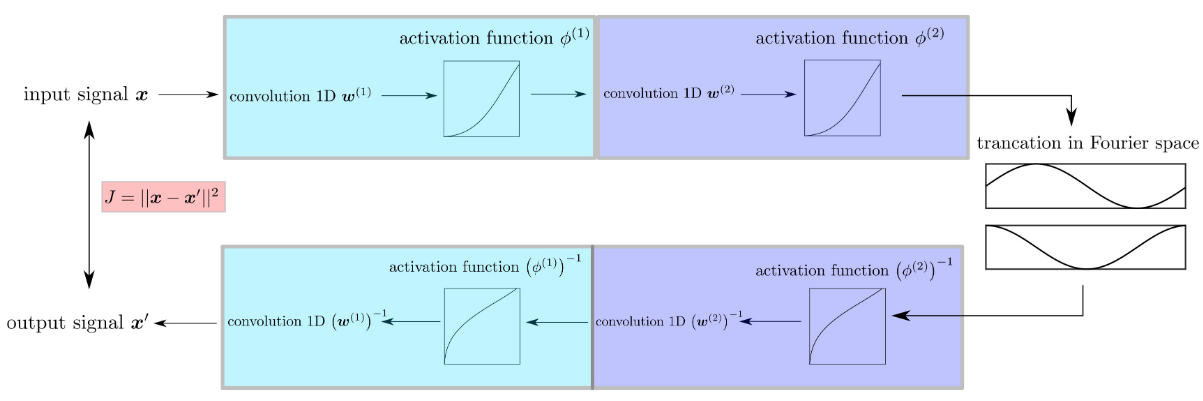
Figure 1: Schematic of the FINE architecture.

In order to determine the structural constraints imposed by translation equivariance under cyclic permutation of inputs, we look at the form of the universal approximation theorem of arbitrary depth, which yields the following sufficient condition: a) linear convolutions $\boldsymbol{w}$, b) Elementwise activation $\phi$’s (Yu et al., 2021). We apply this architecture into nested layers and write our encoder network structure as

$$\boldsymbol{g}_{e}(\boldsymbol{x})=\boldsymbol{z}=\mathcal{P}_{\mathcal{F}}\phi^{(L)}\left(\mathbf{w}^{(L)}\circ\boldsymbol{\phi}^{(L-1)}\left(\mathbf{w}^{(L-1)}\circ\cdots\phi^{(1)}\left(\mathbf{w}^{(1)}\circ\mathbf{x}\right)\cdots\right)\right)$$ (1)

where $\mathcal{P}_{\mathcal{F}}$ is a Fourier truncation projection operator. The corresponding decoder would be

$$\boldsymbol{x}^{\prime}=\boldsymbol{g}_{d}(\boldsymbol{z})=\left(\mathbf{w}^{(1)}\right)^{-1}\circ(\phi^{(1)})^{-1}\circ\left(\mathbf{w}^{(2)}\right)^{-1}\circ(\phi^{(2)})^{-1}\circ\cdots\circ\left(\mathbf{w}^{(L)}\right)^{-1}\circ(\phi^{(L)})^{-1}(\boldsymbol{z})$$ (2)

This procedure is shown in schematic 1. Ensuring the invertibility of the decoder introduces two key technical requirements: the activation functions must be strictly monotonic to admit well-defined inverses, and the convolution filters must have non-zero Fourier coefficients at all frequencies to guarantee invertibility in the spectral domain.

2.1 Invertible activations

We define an invertible activation function based on a residual formulation that applies identically across the spatial domain. the activation is defined as $\phi(x_{i})=x_{i}+\alpha\,\varphi(x_{i})$, where $\varphi:\mathbb{R}\to\mathbb{R}$ is a learnable nonlinear function, and $\alpha>0$ is a small scaling factor. Invertibility of the activation $\phi$ is guaranteed if the residual function $\varphi$ is Lipschitz continuous with constant $L$, and the scaling parameter satisfies $\alpha L<1$. This can be done using spectral normalization. Under these conditions, $\phi$ is strictly monotonic for each coordinate, and the inverse $\phi^{-1}(y_{i})$ exists and can be computed via fixed-point iteration:

$$x_{i}^{(k+1)}=y_{i}-\alpha\,\varphi(x_{i}^{(k)}),$$

initialized with $x_{i}^{(0)}=y_{i}$. Convergence follows from the contraction mapping principle, due to the small Lipschitz perturbation. Translation equivariance is naturally preserved. Since $f$ is applied identically to each coordinate $x_{i}$ without referencing absolute position. Moreover, because the activation operates elementwise and independently on each signal coordinate, invertibility depends only on the local properties of $\varphi$ and the scalar $\alpha$, not on the global dimension $n$ of the input. Thus, changes in the dimensionality of the signal outside the activation block—such as those induced by spectral truncation or zero-padding—do not affect the fundamental invertibility of the activation.

2.2 Monotonic activation functions using ReLU

To preserve invertibility throughout the network, each activation function $\phi$ in the encoder must be strictly monotonic, allowing its inverse $(\phi)^{-1}$ to be well-defined in the decoder. A particularly effective and computationally efficient class of invertible activations is monotonic piecewise linear functions, which can be constructed using compositions of ReLU functions.

To ensure invertibility and stable gradient propagation, we employ a smooth approximation of ReLU that preserves differentiability across the activation domain, termed $\text{SmoothReLU}_{\varepsilon}(x)$. This function transitions smoothly from zero to linear behavior using a cubic Hermite interpolation over a small transition band $[-\varepsilon,\varepsilon]$, controlled by a parameter $\varepsilon>0$. The $\text{SmoothReLU}_{\varepsilon}(x)$ is defined as

$$\text{SmoothReLU}_{\varepsilon}(x)=x\cdot h\left(\frac{x+\varepsilon}{2\varepsilon}\right),\quad\text{where}\quad h(t)=t^{2}\left(3-2t\right)$$ (3)

Here, $t=\frac{x+\varepsilon}{2\varepsilon}$ maps $x\in[-\varepsilon,\varepsilon]$ to $[0,1]$. Outside this transition band, $\text{SmoothReLU}_{\varepsilon}(x)$ exactly matches the standard ReLU behavior, while inside, the cubic Hermite interpolation ensures differentiability and strict monotonicity between $(0,0)$ and $(1,1)$. Thus, our method can be interpreted as a smooth and stable approximation of the cumsum(exp(z)) activation family, tailored for piecewise linear interpolation with invertibility.

2.3 Invertible Filters

Convolutional filters must be invertible to ensure the encoder–decoder pair remains bijective. This is equivalent to requiring that their Fourier transform $\hat{w}(k)$ has no zero entries for any frequency $k\in[0,2\pi)$, thus preserving all spectral modes. In our implementation, we enforce this by parameterizing the filters in the frequency domain and regularizing the magnitude of $\hat{w}(k)$ away from zero. The decoder applies inverse filtering in the spectral domain, allowing exact reconstruction via elementwise division in the Fourier space. The filtered signal is obtained by elementwise multiplication in the frequency domain, followed by an inverse Fourier transform $z_{\text{spatial}}=\mathcal{F}^{-1}\left(\hat{w}\odot\mathcal{F}(x)\right)$.

Training When all filters and activation functions are set to identity, the autoencoder reduces exactly to a Fourier truncation operator. Motivated by this observation, we initialize the network with identity filters and activation functions, and perform training using full-batch optimization. Due to the novelty of the architecture, we observed instability and insufficient convergence when using standard training strategies such as minibatch updates or randomized initializations. As this work represents the first exploration of this type of network, developing more robust and efficient training procedures remains an important direction for future research.

3 Experiments

3.1 Toy problem

The first example investigated is a synthetic one-dimensional signal defined by

$$f(x;\boldsymbol{\omega})=\tanh\Bigl{(}\sin\bigl{(}x+\omega_{1}+\cos(2x+\omega_{2})\bigr{)}\Bigr{)}$$

where $\boldsymbol{\omega}=(\omega_{1},\omega_{2})\in\Theta=[0,2\pi)^{2}$ denotes the phase of two nonlinearly interacting waveforms, and $x\in[0,2\pi)$ is the independent variable. The dataset is generated by randomly sampling 100 different parameter sets $\boldsymbol{\omega}$, and evaluating the corresponding signals on a uniform grid of 128 points in $x\in[0,2\pi)$. This dataset is particularly well-suited for our study for several reasons. First, the underlying latent space is two-dimensional and periodic in both directions, naturally forming a torus topology. Recovering this toroidal structure is an essential challenge for any method aiming to uncover meaningful low-dimensional representations of the data. Second, the signal is highly nonlinear due to the nested sine and cosine functions and the outer hyperbolic tangent, leading to nontrivial interactions between frequency components.

Traditional linear decomposition methods, which all result in the discrete Fourier transform (DFT), fail to capture the underlying structure of the data. In particular, the energy spectrum obtained from the FFT suggests that the second harmonic is entirely absent—despite the fact that a term with wave number 2 is present inside the composition. The nonlinear composition effectively cancels out the signal with wave number $2$. This highlights the limitations of linear methods in representing data governed by nonlinear and phase-dependent systems, and motivates the use of more expressive tools capable of resolving hidden geometric and topological features in function space.

The goal of this toy problem is to evaluate how different autoencoder architectures compress and reconstruct structured, nonlinear signals using a low-dimensional latent space. In all experiments, the latent dimension is 2, recognizing that the zero wavenumber component is consistently $0$ across the dataset.

We compare the FINE model with conventional CNN-based down-sampling and up-sampling autoencoders, consisting of a stack of 1D convolutions, max-pooling layers, and transposed convolutions, as shown in figure 2 (left). Figure 2 also shows the IResNet-based FINE architecture. The FINE architecture uses two monotonic activation layers surrounding a spectral filter and leverages Fourier-based truncation to form interpretable latent variables.

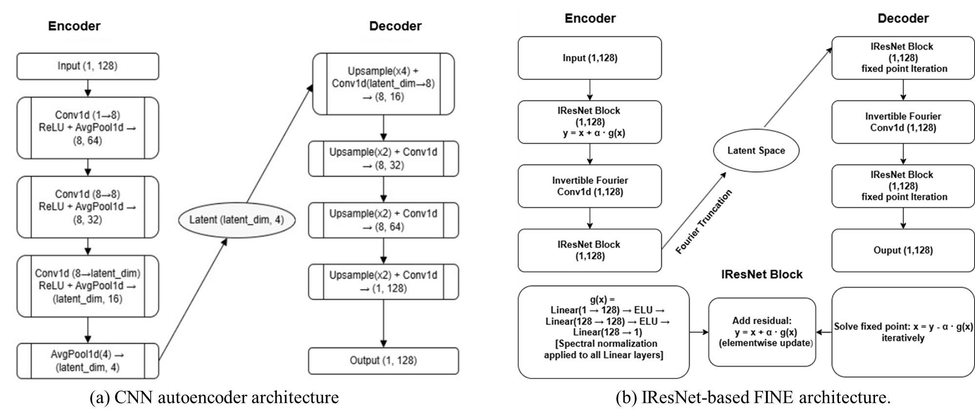
Figure 2: Architectures of the models.

Loss Curve Comparison Figure 6(a) shows the training loss curve of the CNN autoencoder over 4000 epochs. The training begins with a high loss of approximately 2800 and decreases rapidly during the initial phase (first 500 epochs), indicating that the model quickly captures coarse features of the signal. Subsequently, the loss continues to decrease gradually, reaching a value of 430 at epoch 4000. To complement this analysis, we compare the final reconstruction losses of CNN and FINE models across varying latent dimensions, as illustrated in Figure 6(a). The FINE model achieves near-zero reconstruction loss with as few as 8 latent dimensions, and the loss remains at machine precision for all higher dimensions. In contrast, the CNN model requires significantly more latent capacity to reduce the loss, and even at dimension 64, it fails to match FINE’s performance. These results highlight FINE’s superior ability to extract and represent essential latent features efficiently, demonstrating its effectiveness in capturing the underlying structure of the signal with fewer parameters.

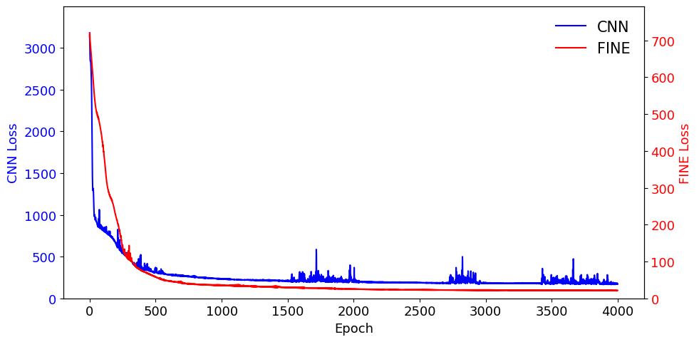
(a) Training loss on Toy Problem 1.

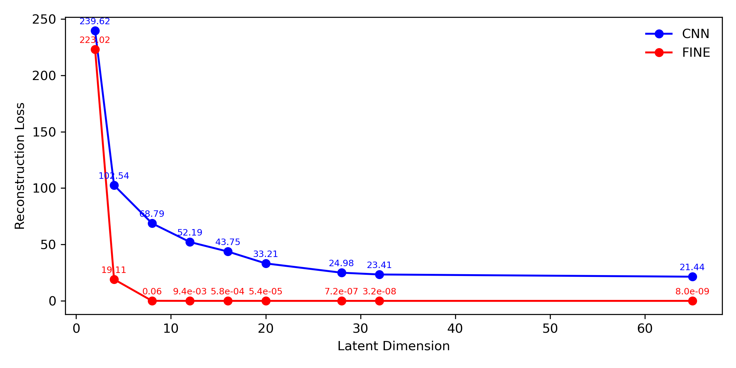
(b) Reconstruction loss vs. dimension.

Figure 3: Comparison of training dynamics and dimensionality impact on loss.

In contrast, the training loss curve of the FINE model is shown in Figure 6(a). The FINE model starts with a significantly lower initial loss of 709.5 and rapidly converges to below 100 within the first 300 epochs. While a brief spike occurs near epoch 500, likely due to a temporary instability in the Fourier filter inversion, the overall convergence is faster and smoother compared to the CNN model.

Reconstruction Quality at Convergence To qualitatively assess the final reconstruction ability of the two models, we visualize a representative test signal reconstructed at the end of training (epoch 4000). Each figure overlays three curves: the original signal, the Fourier-truncated version (retaining only the dominant low-frequency components), and the model’s reconstructed output.

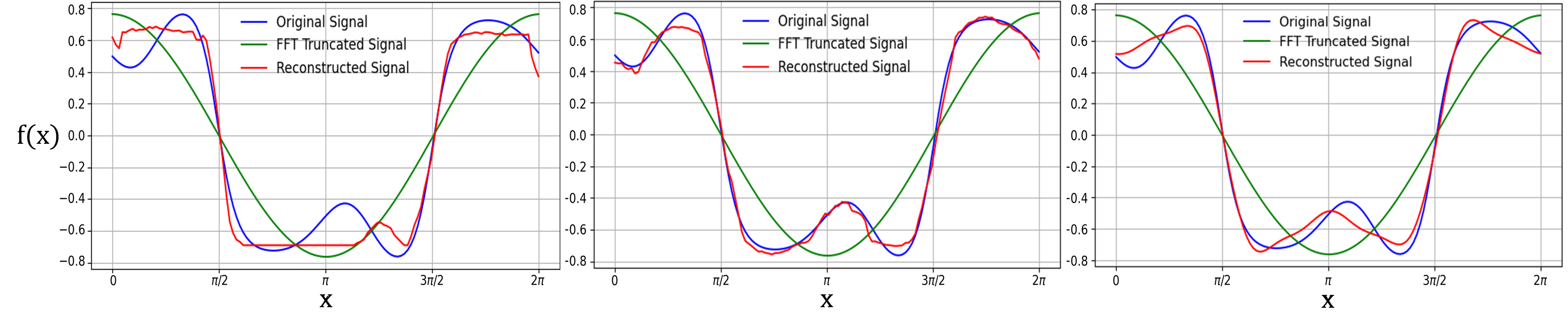
(a) CNN autoencoder reconstruction. (b) FINE Reconstruction. (c) IResNet Reconstruction.

Figure 4: Reconstruction results on the Toy Problem 1.

Figure 4 compares the reconstructed signals of the CNN-based autoencoder (left), the FINE model (center), and the iResNet-based model (right) after 4000 epochs, each using a 2-dimensional latent representation. The CNN reconstruction roughly follows the shape of the target waveform but shows underfit regions of rapid variation, particularly near local extrema. These discrepancies suggest that the CNN struggles to encode the global structure effectively when constrained to a low-dimensional latent space.

In contrast, the FINE model reconstructs the signal with significantly higher fidelity. It accurately preserves the phase, amplitude, and harmonic content, closely matching the original waveform even in high-frequency regions. Despite having fewer parameters than the CNN, FINE benefits from its invertible architecture and Fourier-aware latent structure. This comparison underscores the limitations of conventional CNN autoencoders for structured signals and highlights the representational efficiency of FINE.

As an additional baseline, we also evaluated an iResNet-based autoencoder. The iResNet model achieves a notably improved reconstruction over the CNN, accurately capturing local extrema and waveform smoothness. Although slightly less precise than the FINE model in high-frequency regions, it demonstrates that invertible architectures are effective in low-dimensional latent spaces even without explicit spectral structure. This further reinforces the advantage of the FINE design, which combines invertibility with Fourier-domain awareness to reach superior reconstruction fidelity.

Table 1: Comparison of performance metrics between CNN and FINE on Toy Problem 1.

Metric	CNN	FINE	Gain (FINE/CNN)
Parameters	812	174	0.21×
CPU Time (s)	14.82	120.23	8.11×
MSE	169.71	21.37	0.13×

Table 1 summarizes the performance of the proposed FINE model compared to a conventional CNN on Toy Problem 1. While FINE requires significantly longer training time (approximately 8× in CPU time), this is an expected outcome given the model’s architectural constraints and initialization strategy, as discussed in previous sections. Despite the increased training cost, FINE achieves substantially improved accuracy, with the mean squared error (MSE) reduced to approximately 13% of that of CNN, and it does so with only about 21% of the trainable parameters. These results reflect a trade-off between computational efficiency and model interpretability: FINE imposes structural biases that better capture the underlying symmetries of the data, making it particularly suitable for applications where understanding the learned representation is as important as predictive performance.

3.2 One-dimensional turbulence in Kuramoto–Sivashinsky equation

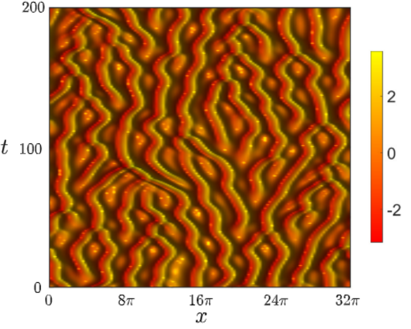
Figure 5: Sample evolution of the K-S equation within a time horizon of $200$.

The Kuramoto–Sivashinsky (K-S) equation, $\frac{\partial u}{\partial t}+u\frac{\partial u}{\partial x}+\frac{\partial^{2}u}{\partial x^{2}}+\nu\frac{\partial^{4}u}{\partial x^{4}}=0,$ is a canonical one-dimensional nonlinear partial differential equation used to model instabilities in laminar flame fronts, reaction-diffusion systems, and thin film flows. It exhibits chaotic dynamics with spatiotemporal complexity, making it a widely used testbed for studying low-dimensional models of turbulence. We solve the K-S equation on a periodic domain with 128 uniformly spaced spatial points and sample 100 temporal snapshots from a single trajectory of temporal length $10^{4}$, as can be partially seen in figure 5. Each snapshot corresponds to a different realization drawn from the underlying turbulent distribution, forming a dataset with translation-equivariant structure.

The signals contain rich multiscale features and high-frequency fluctuations, providing a challenging benchmark for nonlinear model reduction. As in the previous toy problem, the goal is to evaluate whether different autoencoder architectures can effectively compress and reconstruct these structured dynamics using a low-dimensional latent space of 10.

Table 2: Comparison of performance metrics between the CNN and FINE models on K-S Problem.

Metric	CNN	FINE	Gain (FINE/CNN)
Parameters	1496	174	0.12×
CPU Training Time (s)	7.23	80.72	11.16×
GPU Training Time (s)	5.09	56.86	11.17×
MSE	2669.23	550.30	0.21×

Loss Curve Comparison

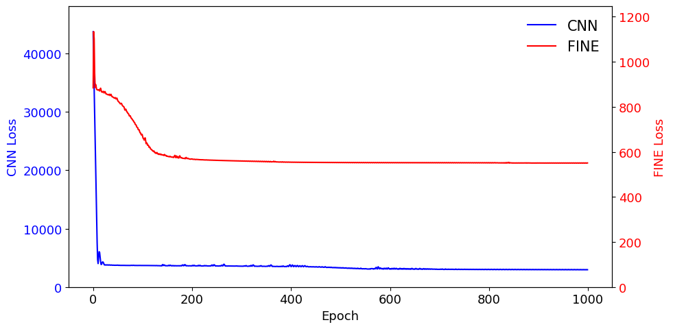
(a) Training loss on the solution of K-S equation.

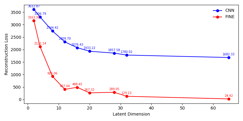
(b) Reconstruction loss vs. dimension.

Figure 6: Comparison of training dynamics and dimensionality impact on loss.

Figure 6 shows the training loss of both models over 1000 epochs. The CNN autoencoder starts at a high initial loss of over 26,000 and gradually decreases to around 2,600. Its loss curve exhibits slow convergence and frequent fluctuations. In contrast, the FINE model begins at a significantly lower initial loss ( 884.4) and steadily decreases to approximately 556 by epoch 1000, achieving both faster convergence and lower final loss.

Reconstruction Quality at Convergence We evaluate the reconstruction performance of both models at epoch 1000 using a representative K-S snapshot. Each figure overlays the ground truth signal, its Fourier-truncated baseline, and the reconstructed output.

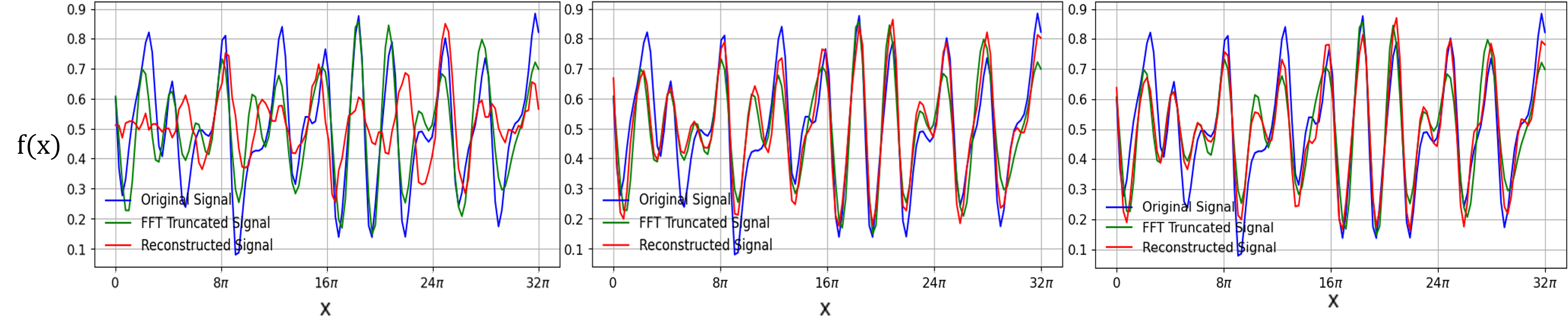
(a) CNN autoencoder reconstruction. (b) FINE Reconstruction. (c) IResNet Reconstruction.

Figure 7: Reconstruction result on the 1D Kuramoto–Sivashinsky dataset.

Figure 7 shows the reconstruction results of the CNN-based autoencoder (left), the FINE model (center), and the iResNet-based model (right) on a signal with sharper local features derived from the Kuramoto–Sivashinsky (KS) equation. The CNN reconstruction captures the overall trend but significantly smooths the amplitude envelope, particularly in high-frequency regions. Sharp peaks are often damped or misaligned, indicating the difficulty of CNN to retain critical turbulent modes under severe dimensional compression. The FINE reconstruction exhibits precise alignment with the original waveform. It successfully recovers both dominant and localized features, closely tracking rapid transitions and preserving high-frequency components. Compared to the Fourier-truncated baseline, FINE offers superior sharpness and phase fidelity, demonstrating the effectiveness of invertible spectral filtering and monotonic nonlinearities in structured signal modeling. In comparison, the iResNet-based model achieves comparable reconstruction quality, showing that invertible networks with elementwise updates can effectively model nonlinear dynamics. Nevertheless, FINE remains the core contribution—its structured spectral filtering and monotonic activations yield sharper reconstructions and better capture translation symmetry. These results affirm FINE’s extensibility and effectiveness for learning low-dimensional representations of turbulent signals.

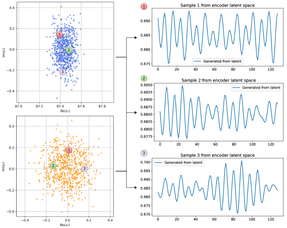
(a) Latent space distribution

(b) Generated fields from sampled latent vectors

Figure 8: Visualization of the FINE model’s latent space and its decoding capacity on K-S Problem.

Figure 8 illustrates the latent space distribution learned by the FINE model for the one-dimensional Kuramoto-Sivashinsky (K-S) problem. Each subplot corresponds to a different complex-valued latent variable: the left plot shows the distribution of $z_{1}$ and the right plot shows $z_{2}$, on a complex plane. Notably, both latent variables exhibit a Gaussian distribution in the latent space and remain uncorrelated. This suggest a behavior similar to $\beta-$variational auto-encoder (Solera-Rico et al., 2024) and the FINE architecture, once decomposed into Fourier modes in the latent space, marks independent coordinates of the dataset and might have a generative nature.

4 Conclusion and Future work

We propose a novel autoencoder framework composed entirely of invertible neurons, with the exception of a Fourier truncation operator in the bottleneck. This architecture naturally preserves translation equivariance, making it particularly well-suited for data arising from physical simulations. The fully invertible activation functions can either be approximated using ReLu, or using an invertible-ResNet structure. We evaluate the framework adopting both approaches on two one-dimensional problems: a toy example involving two nonlinearly interacting waves, and the statistically stationary solution of the Kuramoto–Sivashinsky (K–S) equation. Results show that FINE achieves superior reconstruction accuracy using simpler network structures and fewer parameters, while offering a more interpretable latent space compared to linear methods and conventional CNN-based downsampling and upsampling schemes. These findings highlight the potential of invertible networks and flexible activation functions in scientific machine learning. Future work includes a solid mathematical investigation of the convergence and stability behavior of FINE, and generalization of this framework to two and three dimensional dataset from turbulent simulations.

References

- Park and Lozano-Durán [2025] Danah Park and Adrián Lozano-Durán. The coherent structure of the energy cascade in isotropic turbulence. Scientific Reports, 15(1):14, 2025.
- Motoori and Goto [2021] Yutaro Motoori and Susumu Goto. Hierarchy of coherent structures and real-space energy transfer in turbulent channel flow. Journal of Fluid Mechanics, 911:A27, 2021.
- Worrall et al. [2017] Daniel E. Worrall, Stephan J. Garbin, Daniyar Turmukhambetov, and Gabriel J. Brostow. Harmonic networks: Deep translation and rotation equivariance. arXiv preprint arXiv:1612.04642, 2017.
- Thomas et al. [2018] Nathaniel Thomas, Tess Smidt, Steven Kearnes, Lusann Yang, Li Li, Kai Kohlhoff, and Patrick Riley. Tensor field networks: Rotation- and translation-equivariant neural networks for 3d point clouds. arXiv preprint arXiv:1802.08219, 2018.
- Eyink [2024] Gregory Eyink. Onsager’s ’ideal turbulence’ theory. arXiv preprint arXiv:2404.10084, 2024.
- Johnson [2020] Perry Johnson. Energy transfer from large to small scales in turbulence by multiscale nonlinear strain and vorticity interactions. Physical Review Letters, 124(10):104501, 2020.
- Fukami and Taira [2023] Kai Fukami and Kunihiko Taira. Grasping extreme aerodynamics on a low-dimensional manifold. Nature Communications, 14(1):1–11, 2023.
- Fukami and Taira [2024] Kai Fukami and Kunihiko Taira. Single-snapshot machine learning for super-resolution of turbulence. arXiv preprint arXiv:2409.04923, 2024.
- Helwig et al. [2023] Jacob Helwig, Xinyang Zhang, Chengyue Fu, Joshua Kurtin, Samy Wojtowytsch, and Shi Jin. Group equivariant fourier neural operators for partial differential equations. arXiv preprint arXiv:2306.05697, 2023.
- Jimenez [2018] Javier Jimenez. Coherent structures in wall-bounded turbulence. arXiv preprint arXiv:1710.07493, 2018.
- Doan et al. [2023] Nguyen Anh Khoa Doan, Andrea Racca, and Luca Magri. Convolutional autoencoder for the spatiotemporal latent representation of turbulence. arXiv preprint arXiv:2301.13728, 2023.
- Li et al. [2024] Zongyi Li, Dezhi Zhang Huang, Burigede Liu, and Anima Anandkumar. Fourier neural operator with learned deformations for pdes on general geometries. arXiv preprint arXiv:2207.05209, 2024.
- Lumley [1967] John L. Lumley. The structure of inhomogeneous turbulent flows. In A. M. Yaglom and V. I. Tatarski, editors, Atmospheric Turbulence and Radio Wave Propagation, pages 166–177. Nauka, Moscow, 1967.
- Abdi and Williams [2010] Hervé Abdi and Lynne J Williams. Principal component analysis. Wiley Interdisciplinary Reviews: Computational Statistics, 2(4):433–459, 2010.
- Schmid [2010] Peter J Schmid. Dynamic mode decomposition of numerical and experimental data. Journal of Fluid Mechanics, 656:5–28, 2010.
- Towne et al. [2018] Aaron Towne, Oliver T Schmidt, and Tim Colonius. Spectral proper orthogonal decomposition and its relationship to dynamic mode decomposition and resolvent analysis. Journal of Fluid Mechanics, 847:821–867, 2018.
- Bolla et al. [2021] Marianna Bolla, Tamás Szabados, Máté Baranyi, and Fatma Abdelkhalek. Block circulant matrices and the spectra of multivariate stationary sequences. Special Matrices, 9(1):36–51, 2021. doi:10.1515/spma-2020-0121.
- Lusch et al. [2018] Bethany Lusch, J Nathan Kutz, and Steven L Brunton. Deep learning for universal linear embeddings of nonlinear dynamics. Nature Communications, 9(1):4950, 2018. doi:10.1038/s41467-018-07210-0.
- Hinton and Salakhutdinov [2006] Geoffrey E Hinton and Ruslan R Salakhutdinov. Reducing the dimensionality of data with neural networks. science, 313(5786):504–507, 2006.
- Cohen and Welling [2016] Taco S. Cohen and Max Welling. Group equivariant convolutional networks. arXiv preprint arXiv:1602.07576, 2016.
- Kingma and Welling [2014] Diederik P. Kingma and Max Welling. Auto-encoding variational bayes. arXiv preprint arXiv:1312.6114, 2014.
- Azencot et al. [2020] Omri Azencot, Nathan Erichson, and Michael Mahoney. Forecasting sequential data using consistent koopman autoencoders. arXiv preprint arXiv:2006.02548, 2020.
- Liu et al. [2025] Ziming Liu et al. Kan: Kolmogorov–arnold networks. arXiv preprint arXiv:2404.19756, 2025.
- Yu et al. [2021] Annan Yu, Chloé Becquey, Diana Halikias, Matthew Esmaili Mallory, and Alex Townsend. Arbitrary-depth universal approximation theorems for operator neural networks. arXiv preprint arXiv:2109.11354, 2021.
- Solera-Rico et al. [2024] Alberto Solera-Rico, Carlos Sanmiguel Vila, Miguel Gómez-López, Yuning Wang, Abdulrahman Almashjary, Scott TM Dawson, and Ricardo Vinuesa. -variational autoencoders and transformers for reduced-order modelling of fluid flows. Nature Communications, 15(1):1361, 2024.