Testing for replicated signals across multiple studies with side information

Abstract.

Partial conjunction (PC) $p$-values and side information provided by covariates can be used to detect signals that replicate across multiple studies investigating the same set of features, all while controlling the false discovery rate (FDR). However, when many features are present, the extent of multiplicity correction required for FDR control, along with the inherently limited power of PC $p$-values—especially when replication across all studies is demanded—often inhibits the number of discoveries made. To address this problem, we develop a $p$-value-based covariate-adaptive methodology that revolves around partitioning studies into smaller groups and borrowing information between them to filter out unpromising features. This filtering strategy: 1) reduces the multiplicity correction required for FDR control, and 2) allows independent hypothesis weights to be trained on data from filtered-out features to enhance the power of the PC $p$-values in the rejection rule. Our methodology has finite-sample FDR control under minimal distributional assumptions, and we demonstrate its competitive performance through simulation studies and a real-world case study on gene expression and the immune system.

1. Introduction

The widespread “replicability crisis” has gained significant attention in contemporary scientific research (Pashler and Harris,, 2012), and the recent article of Bogomolov and Heller, (2023) has provided a timely review on the latest developments in testing for replicable research findings. The general problem setting can be described by a meta-analytical framework that consists of $n$ comparable studies, each examining the same set of $m$ features. Adopting the shorthand $[\ell]\equiv\{1,\dots,\ell\}$ for any natural number $\ell\in\mathbb{N}\equiv\{1,2,\dots\}$, suppose $\mu_{ij}\in\mathbb{R}$ is an unknown effect parameter corresponding to feature $i\in[m]$ in study $j\in[n]$, and $\mathcal{A}_{i}\subseteq\mathbb{R}$ is a common null parameter region across the $n$ studies for feature $i$. The effect specific to study $j$ is considered a scientifically interesting finding (i.e., a signal) if $\mu_{ij}$ does not belong to $\mathcal{A}_{i}$. Consequently, the query of whether $\mu_{ij}$ is a signal can be formulated as testing the null hypothesis

$$H_{ij}:\mu_{ij}\in\mathcal{A}_{i}$$

against the alternative $\mu_{ij}\not\in\mathcal{A}_{i}$. In this paper, we exemplify the problem with a meta-analysis on thymic gene differential expression in relation to autoimmunity, the details of which will be given in Section 5.

Example 1.1 (Meta-analysis on differential gene expression in thymic medulla for autoimmune disorder).

We consider a meta-analysis on RNA-Seq data obtained from medullary thymic epithelial cells (mTECs) for $m=6,587$ genes compiled from $n=3$ independent mouse studies. For each $(i,j)\in[6587]\times[3]$, $\mu_{ij}\in\mathbb{R}$ is the mean difference in expression level of gene $i$ between healthy and autoimmune mice in study $j$. If $\mu_{ij}\neq 0$ (corresponding to $\mathcal{A}_{i}={0}$), then gene $i$ in study $j$ is implicated as a potential marker for autoimmunity, as its expression differs between healthy and autoimmune mice, on average.

As a simple starting point, we assume the primary data available from the studies allow a statistician to directly access or otherwise construct a $p$-value $p_{ij}$ to test $H_{ij}$ for each $(i,j)\in[m]\times[n]$. For meta-analyses like Example 1.1, the gene expression data are often available on public repositories such as the Gene Expression Omnibus (GEO) and can be processed into $p$-values using bioinformatics pipelines like limma Ritchie et al., (2015) in R. We further assume the statistician has access to side information in the form of a covariate $x_{ij}$ that is also relevant for testing $H_{ij}$; for instance, in Example 1.1, $x_{ij}$ can be taken as the differential expression of gene $i$ in cells from a different part of the thymus other than the medulla, such as the cortex as described in Section 5. This latter assumption reflects the recent trend of hypothesis testing methods evolving from relying solely on $p$-values to integrating side information to improve power; see Lei and Fithian, (2018), Ignatiadis and Huber, (2021), and Zhang and Chen, (2022) for examples. For compactness, we will use

$$\mathbf{P}\equiv(p_{ij})_{i\in[m],j\in[n]}\quad\text{ and }\quad\mathbf{X}\equiv(x_{ij})_{i\in[m],j\in[n]}$$

to denote the $m\times n$ matrices of these $p$-values and covariates, respectively.

Testing the null hypotheses $H_{ij}$ is certainly front and central to each study; however, to enforce some notion of generalizability for scientific findings, one may demand more and ask whether a given feature $i$ has replicated signals across studies. The following paradigm, first advocated by Friston et al., (2005), Benjamini and Heller, (2008) and Benjamini et al., (2009), addresses the latter problem: For a given number $u\in[n]$ that represents the required level of replicability, declare the effect of feature $i$ as being $u/[n]$ replicated if at least $u$ of $\mu_{i1},\dots,\mu_{in}$ are signals. This can be formulated as testing the partial conjunction (PC) null hypothesis

(1.1) $$H^{u/[n]}_{i}:|\{j\in[n]:\mu_{ij}\in\mathcal{A}_{i}\}|\geq n-u+1$$

which states that at least $n-u+1$ of the effects $\mu_{i1},\dots,\mu_{in}$ belong to the null set $\mathcal{A}_{i}$, or equivalently, no more than $u-1$ of $\mu_{i1},\dots,\mu_{in}$ are signals. Setting $u=1$ amounts to testing the global null hypothesis that $H_{ij}$ is true for all $j\in[n]$, an inferential goal pursued in many past meta-analyses, but one that is the least demanding in terms of replicability. At the other end, setting $u=n$, the maximum replicability level, offers the strictest, yet most conceptually appealing, benchmark for assessing the generalizability of scientifically interesting findings.

As the number of features $m$, such as the number of genes examined in Example 1.1, is typically large, it is natural to apply procedures that aim to control the false discovery rate (FDR) while testing the PC null $H_{i}^{{}_{u/[n]}}$ for all features $i\in[m]$ en masse. In the present context of assessing $u/[n]$ replicability, suppose $\widehat{\mathcal{R}}\subseteq[m]$ is a set of rejected PC nulls determined based on the available data $\mathbf{P}$ and $\mathbf{X}$; the FDR for $\widehat{\mathcal{R}}$ is defined as

$$\text{FDR}_{\text{rep}}=\text{FDR}_{\text{rep}}(\widehat{\mathcal{R}})\equiv\mathbb{E}\left[\frac{\sum_{i\in\mathcal{H}^{u/[n]}}I\{i\in\widehat{\mathcal{R}}\}}{1\vee\sum_{i\in[m]}I\{i\in\widehat{\mathcal{R}}\}}\right],$$

where $a\vee b\equiv\max(a,b)$ for any real numbers $a,b\in\mathbb{R}$ and

$$\mathcal{H}^{u/[n]}\equiv\{i\in[m]:H_{i}^{u/[n]}\text{ is true}\}$$

is the set of all features whose PC null hypotheses are true. In other words, $\text{FDR}_{\text{rep}}$ is the expected proportion of Type I errors made by rejecting the PC nulls associated with the features in $\widehat{\mathcal{R}}$.

In this work, we aim to develop a new method with strong theoretical $\text{FDR}_{\text{rep}}$ control for testing the $m$ PC nulls in (1.1), with an emphasis on the most appealing but power-deprived replicability level $u=n$. A standard protocol for controlling the $\text{FDR}_{\text{rep}}$ is to apply the widely-used Benjamini-Hochberg (BH) procedure (Benjamini and Hochberg,, 1995) to a set of $m$ $p$-values for assessing the PC nulls, also commonly referred to as partial conjunction (PC) $p$-values. In the literature, a PC $p$-value for testing $H_{i}^{{}_{u/[n]}}$, denoted as $p^{{}_{u/[n]}}_{i}$, is typically constructed by combining $p_{i1},\dots,p_{in}$ (i.e., the base $p$-values for feature $i$) following the formulation proposed by Benjamini and Heller, (2008) and later extended by Wang and Owen, (2019); see our review in Section 2. Although seemingly natural, this approach is often severely underpowered for a high replicability level such as $u=n$. Figure 1.1 previews the results of a simulation experiment in Section 2.1 and shows that the power for assessing $u=n=4$ replicability can quickly diminish toward zero as $m$ increases, while the power for other replicability levels, $u<n$, can remain high and stable. One reason is the expansion of the null parameter space of $H^{u/[n]}_{i}$ for each $i\in[m]$ as $u$ increases (Bogomolov,, 2023, Sec. 2.1). Another reason is that the multiplicity correction applied by the BH procedure can disproportionately reduce power for $u=n$ compared to other replicability levels.

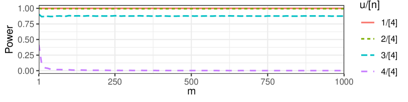
Figure 1.1. Power of the BH procedure (with FDR target $0.05$) applied to $m=1,10,20,\cdots,1000$ PC $p$-values under replicability levels $u=1,2,3,4$, based on a simulation experiment with a total of $n=4$ studies. By design, $H^{u/[n]}_{i}$ is false for each $(i,u)\in[m]\times[4]$, and its corresponding PC $p$-value $p^{u/[4]}_{i}$ is constructed from the base $p$-values $p_{i1},\dots,p_{i4}$ using the generalized Benjamini–Heller formulation in Definition 2, with Stouffer’s combining function (Stouffer et al.,, 1949); see Section 2 for more details.

Our new method is called ParFilter, as an acronym for partitioning and filtering, which characterizes the main idea behind our approach: the ParFilter partitions the $n$ studies into different groups and borrows information between these groups to filter out features that are unlikely to be $u/[n]$ replicable. Subsequently, a rejection rule with multiple thresholds, one for each group, is applied to combined $p$-values to form rejections for declaring $u/[n]$ replicability. This filtering process is advantageous because it: (1) reduces the required multiplicity correction, and (2) allows independent hypothesis weights to be trained on data from filtered-out features to enhance the power of the combined $p$-values.

The idea of filtering out unpromising features to alleviate the multiplicity correction is certainly not new in multiple testing. In partial conjunction hypothesis testing, one state-of-the-art method employing this strategy is the AdaFilter-BH procedure (Wang et al.,, 2022). In a nutshell, this method first filters out unpromising features that are unlikely to exhibit $(u-1)/[n]$ replicability and then computes a final rejection set for $u/[n]$ replicability from the remaining features. This is a natural approach for reducing the multiplicity burden because a feature that is $u/[n]$ replicated is also $(u-1)/[n]$ replicated. Since its rejection set is derived from the same base $p$-values used to construct the filter, AdaFilter-BH offers only asymptotic $\text{FDR}_{\text{rep}}$ control under mild limiting distributional assumptions. In comparison, the ParFilter filters uses stable selection rules that exploit the independence between the $n$ studies to ensure finite-sample $\text{FDR}_{\text{rep}}$ control; see Section 3.2 for details. This type of filter resembles those used in the procedures of Bogomolov and Heller, (2018); these procedures, however, are restricted to assessing $2/[2]$ replicability only, whereas the ParFilter accommodates arbitrary choices of $u$ and $n$.

On the topic of hypothesis weighting, this technique has long been used in the multiple testing literature to enhance the power of testing procedures by rescaling $p$-values to prioritize the rejection of non-null hypotheses; see Benjamini and Hochberg, (1997), Genovese et al., (2006), and Ignatiadis and Huber, (2021) for notable examples. A data-driven hypothesis weight is said to be independent if it does not depend on the corresponding $p$-value it rescales—a property crucial for avoiding inflated error rates due to data dredging. Ignatiadis and Huber, (2021) proposed a technique for creating independent hypothesis weights by cross-training them on independent data folds. Similarly, the ParFilter cross-trains hypothesis weights on a subset of the data corresponding to the features it filters out. By design, this subset (or “fold”) is independent of the $p$-values to be rescaled in the rejection rule; see Section 3.4 for details. Such a strategy may not be implementable in other $\text{FDR}_{\text{rep}}$ methodologies that employ filtering—for example, the AdaFilter-BH procedure mentioned earlier uses a filter that does not yield independent data folds.

The structure of our work is as follows: Section 2 formally introduces PC $p$-values and examines their power limitations when testing PC nulls at the maximum replicability level ($u=n$). Section 3 provides a detailed overview of the ParFilter, outlining its implementation and finite-sample FDR guarantees (Theorems 3.3 and 3.4). Section 4 demonstrates the competitiveness of the ParFilter against existing $\text{FDR}_{\text{rep}}$ procedures using simulated data. Section 5 explores the ParFilter’s performance in a real replicability analysis based on Example 1.1. Finally, Section 6 concludes with a discussion on potential extensions. An R package implementing the ParFilter is available at https://github.com/ninhtran02/Parfilter.

1.1. Notation

$\Phi(\cdot)$ denotes a standard normal distribution function. For two vectors ${\bf a}$ and ${\bf b}$ of the same length, $\textbf{a}\preccurlyeq\textbf{b}$ (resp. $\textbf{a}\succcurlyeq\textbf{b}$) denotes that each element in a is less (resp. greater) than or equal to its corresponding element in b; for two matrices A and B of equal dimensions, $\textbf{A}\preccurlyeq\textbf{B}$ and $\textbf{A}\succcurlyeq\textbf{B}$ are defined analogously by comparing their corresponding elements. For any two real numbers $a,b\in\mathbb{R}$, $a\vee b\equiv\max(a,b)$ and $a\wedge b\equiv\min(a,b)$. Given a natural number $\ell\in\mathbb{N}$, a real valued function $f:\mathcal{D}\to\mathbb{R}$ defined on a subset $\mathcal{D}\subseteq\mathbb{R}^{\ell}$ is said to be non-decreasing (resp. non-increasing) if $f(\mathbf{x}_{1})\leq f(\mathbf{x}_{2})$ (resp. $f(\mathbf{x}_{1})\geq f(\mathbf{x}_{2})$) for any vectors $\mathbf{x}_{1},\mathbf{x}_{2}\in\mathbb{R}^{\ell}$ such that $\mathbf{x}_{1}\preccurlyeq\mathbf{x}_{2}$. For a vector of real numbers $\mathbf{a}\in\mathbb{R}^{\ell}$, the vector $(1,\mathbf{a})\in\mathbb{R}^{1+{\ell}}$ denotes the concatenation of $1$ and $\mathbf{a}$. For $\ell_{1},\ell_{2}\in\mathbb{N}$ such that $\ell_{1}\leq\ell_{2}$, let $[\ell_{1}:\ell_{2}]\equiv\{\ell_{1},\ell_{1}+1,\dots,\ell_{2}\}$. For a set of numbers $\mathcal{J}\subseteq\mathbb{N}$, let $|\mathcal{J}|$ denote its cardinality.

For an $m\times n$ matrix of base $p$-values $\mathbf{P}$ and a given row $i\in[m]$, $\mathbf{P}_{i\cdot}\equiv(p_{i1},\cdots,p_{in})$ is the $i$th row of $\mathbf{P}$ as a vector. Similarly, for a given column $j\in[n]$, $\mathbf{P}_{\cdot j}\equiv(p_{1j},\cdots,p_{mj})$ is the $j$th column of $\mathbf{P}$ as a vector. More generally, for a subset of columns $\mathcal{J}\subseteq[n]$, $\mathbf{P}_{\cdot\mathcal{J}}$ is a submatrix denoting $\mathbf{P}$ with columns restricted to $\mathcal{J}$, and $\mathbf{P}_{\cdot(-\mathcal{J})}$ is a submatrix denoting $\mathbf{P}$ with columns restricted to $[n]\backslash\mathcal{J}$. If we also have a subset of rows $\mathcal{I}\subseteq[m]$, then $\mathbf{P}_{(-\mathcal{I})\mathcal{J}}$ is a submatrix denoting $\mathbf{P}$ with rows and columns restricted to $[m]\backslash\mathcal{I}$ and $\mathcal{J}$ respectively. Additionally, if $\mathcal{J}=\{j_{1},\dots,j_{|\mathcal{J}|}\}$ is ordered such that $j_{1}\leq\dots\leq j_{|\mathcal{J}|}$, then $\mathbf{P}_{i\mathcal{J}}\equiv(p_{ij_{1}},\dots,p_{ij_{|\mathcal{J}|}})$ is a vector denoting the $i$th row of $\mathbf{P}$ with columns restricted to $\mathcal{J}$.

1.2. Assumptions

The following assumptions regarding the base $p$-values will be invoked throughout this paper:

Assumption 1 (Valid base $p$-values).

Each base $p$-value in $\mathbf{P}\in[0,1]^{m\times n}$ satisfies

$$\Pr(p_{ij}\leq t)\leq t\quad\text{for all $\ t\in[0,1]$ under $H_{ij}$}.$$

In other words, a base $p$-value is stochastically equal to or greater than a uniform distribution (i.e., superuniform) if its corresponding null hypothesis is true.

Assumption 2 (Independence between $p_{ij}$ and $x_{ij}$ under the null).

If $H_{ij}$ is true, then $p_{ij}$ is independent of $x_{ij}$.

Assumption 3 (Independence across studies conditional on $\mathbf{X}$).

Given $\mathbf{X}$, both $\mathbf{P}_{\cdot j}$ and $\mathbf{P}_{\cdot(-j)}$ are independent for each $j\in[n]$. In other words, if $\mathbf{X}$ is given, the base $p$-values in study $j$ are independent of the base $p$-values not in study $j$.

Assumption 1 is a standard property for null $p$-values that underlies FDR control in essentially all $p$-value-based FDR procedures. Assumption 2 is a standard assumption in covariate-assisted testing literature, complementing Assumption 1 by ensuring that the covariates do not influence the null distribution of the base $p$-values; see Ignatiadis and Huber, (2021, Sec. 2.3 and Sup. S6.2) for a more nuanced discussion. Assumption 3 is expected to hold in practice, as meta-analyses typically consist of independently conducted studies.

2. Multiple testing with PC $p$-values

We first review some fundamentals of partial conjunction testing. Consider a generic context where $\theta_{1},\dots,\theta_{n}$ are $n$ parameters of interest and $\Theta_{j}$ is a set of null values for $\theta_{j}$ for each $j\in[n]$. Let $p_{1},\dots,p_{n}\in[0,1]$ be the base $p$-values for testing the null hypothesis $\theta_{1}\in\Theta_{1}$, $\dots$, $\theta_{n}\in\Theta_{n}$ respectively, and suppose these $p$-values are valid, i.e.,

(2.1) $$\Pr(p_{j}\leq t)\leq t\text{ for all }t\in[0,1]\text{ if the null hypothesis }\theta_{j}\in\Theta_{j}\text{ is true}.$$

For a given replicability level $u\in[n]$, the partial conjunction (PC) null hypothesis that at least $n-u+1$ parameters among $\theta_{1},\cdots,\theta_{n}$ are null is denoted as

$$H^{u/[n]}:|\{j\in[n]:\theta_{j}\in\Theta_{j}\}|\geq n-u+1.$$

In the literature, $H^{u/[n]}$ is typically tested by combining the base $p$-values $p_{1},\dots,p_{n}$ to create a combined $p$-value that is both valid and monotonic:

Definition 1 (Valid and monotone combined $p$-values for testing $H^{u/[n]}$).

For a given combining function $f:[0,1]^{n}\to[0,1]$, the combined $p$-value $f(p_{1},\dots,p_{n})$ is said to be

1. valid for testing $H^{u/[n]}$ if $\Pr(f(p_{1},\dots,p_{n})\leq t)\leq t\text{ for all }t\in[0,1]\text{ under $H^{u/[n]}$, and }$

2. monotone if $f$ is non-decreasing.

The combined $p$-value properties outlined in Definition 1 are sought-after because validity is standard for ensuring Type I error control, and monotonicity is sensible for scientific reasoning; a more nuanced discussion on monotonicity can be found in Wang and Owen, (2019, Sec 3.2). For testing $H^{1/[n]}$, i.e., the global null hypothesis that all $\theta_{1}\in\Theta_{1},\dots,\theta_{n}\in\Theta_{n}$ hold true, perhaps the most well-known combining function is

$$f_{\text{Bonferroni}}(p_{1},\dots,p_{n})\equiv(n\cdot\min(p_{1},\dots,p_{n}))\wedge 1.$$

In words, $f_{\text{Bonferroni}}$ applies a Bonferroni correction to the minimum base $p$-value, and the result is usually a very conservative combined $p$-value. Over the last century, more powerful functions for combining $p$-values to test global nulls have been developed, and a comprehensive list of such functions is provided in Bogomolov, (2023, Section 2.1). Below, we present three common choices:

• Fisher, (1973)’s combining function:

  $$f_{\text{Fisher}}(p_{1},\dots,p_{n})\equiv 1-F_{\chi^{2}_{(2n)}}\left(-2\sum_{j\in[n]}\log(p_{j})\right),$$

  where $F_{\chi^{2}_{(2n)}}$ is the chi-squared distribution function with $2n$ degrees of freedom.

• Stouffer et al., (1949)’s combining function:

  $$f_{\text{Stouffer}}(p_{1},\dots,p_{n})\equiv 1-\Phi\left(\frac{\sum_{j\in[n]}\Phi^{-1}(1-p_{j})}{\sqrt{n}}\right);$$

• Simes, (1986)’s combining function:

  $$f_{\text{Simes}}(p_{1},\dots,p_{n})\equiv\min_{j\in[n]}\frac{np_{(j)}}{j},$$

  where $p_{(1)}\leq\dots\leq p_{(n)}$ are the ordered statistics for $p_{1}\leq\dots\leq p_{n}$.

Assuming $p_{1},\dots,p_{n}$ are independent and property (2.1) holds, all four combining functions above (i.e., Bonferroni, Fisher, Stouffer, and Simes) give valid combined $p$-values for testing $H^{1/[n]}$. Moreover, these combining functions are all evidently non-decreasing.

To test $H^{u/[n]}$ for a general $u>1$, the corresponding combined $p$-value, commonly referred to as a PC $p$-value, is typically derived using the generalized Benjamini-Heller combining method (Benjamini and Heller,, 2008, Wang and Owen,, 2019). The resulting PC $p$-value is known as a GBHPC (generalized Benjamini-Heller partial conjunction) $p$-value:

Definition 2 (GBHPC $p$-value for testing $H^{u/[n]}$).

Suppose $u\in[n]$ is given. For each subset $\mathcal{J}=\{j_{1},\dots,j_{n-u+1}\}\subseteq[n]$ of cardinality $n-u+1$ with the ordered elements $1\leq j_{1}<\dots<j_{n-u+1}\leq n$, let

$$\mathbf{P}_{\mathcal{J}}=(p_{j_{1}},\dots,p_{j_{n-u+1}})\text{ and }{\boldsymbol{\theta}}_{\mathcal{J}}=(\theta_{j_{1}},\dots,\theta_{j_{n-u+1}})$$

be the vectors of $p$-values and parameters corresponding to $\mathcal{J}$. Moreover, let $f_{\mathcal{J}}:[0,1]^{n-u+1}\longrightarrow[0,1]$ be a non-decreasing function where $f_{\mathcal{J}}(\mathbf{P}_{\mathcal{J}})$ is valid for testing $H^{1/\mathcal{J}}:{\boldsymbol{\theta}}_{\mathcal{J}}\in\Theta_{j_{1}}\times\cdots\times\Theta_{j_{n-u+1}}$, i.e., the restricted global null hypothesis that all the base nulls corresponding to $\mathcal{J}$ are true. Define the GBHPC $p$-value for testing $H^{u/[n]}$ to be

(2.2) $$f^{\star}(p_{1},\dots,p_{n};u)\equiv\max\{f_{\mathcal{J}}(\mathbf{P}_{\mathcal{J}}):\mathcal{J}\subseteq[n]\text{ such that }|\mathcal{J}|=n-u+1\},$$

i.e., the largest combined $p$-value $f_{\mathcal{J}}(\mathbf{P}_{\mathcal{J}})$ for testing the restricted global nulls $H^{1/\mathcal{J}}$ among all $\mathcal{J}\subseteq[n]$ where $|\mathcal{J}|=n-u+1$.

As a concrete example, if we take each $f_{\mathcal{J}}$ in (2.2) to be Stouffer’s combining function in $n-u+1$ arguments, then

(2.3) $$f^{\star}(p_{1},\dots,p_{n})=f_{\text{Stouffer}}(p_{(n-u+1)},\dots,p_{(n)})=1-\Phi\left(\frac{\sum^{n}_{j=u}\Phi^{-1}(1-p_{(j)})}{\sqrt{n-u+1}}\right).$$

Intuitively, (2.3) makes sense as a $p$-value for testing $H^{u/[n]}$ because it is a function of the largest $n-u+1$ base $p$-values only. GBHPC $p$-values (Definition 2) are valid for testing $H^{u/[n]}$ (Definition 1$(i)$) because every $f_{\mathcal{J}}(\mathbf{P}_{\mathcal{J}})$ in (2.2) is valid for testing their corresponding restricted global null $H^{1/\mathcal{J}}$ (Wang and Owen,, 2019, Proposition 1); moreover, GBHPC $p$-values are monotone (Definition 1$(ii)$) because every $f_{\mathcal{J}}$ in (2.2) is non-decreasing. Additionally, under mild conditions, Wang and Owen, (2019, Theorem 2) demonstrated that any admissible monotone combined $p$-value must necessarily take the form of (2.2).

2.1. The deprived power when $u=n$

Maximum replicability ($u=n$) is the most appealing requirement for ensuring the generalizability of scientific findings; however, it is also the least powerful type of partial conjunction test, because the underlying composite null parameter space of $H^{u/[n]}$ becomes larger as $u$ increases (Bogomolov and Heller,, 2023, Sec. 2.1). What may be surprising is how severely underpowered the case of $u=n$ can be, relative to cases where $u<n$, especially when multiple PC nulls $H_{1}^{{}_{u/[n]}},\dots,H_{m}^{{}_{u/[n]}}$ are tested simultaneously with combined $p$-values. To illustrate, consider a simple scenario with $n=4$ studies, where all the base null hypotheses $H_{ij}$ are false with their corresponding $p$-values generated as

$$p_{ij}\overset{\tiny\text{iid}}{\sim}\text{Beta}(0.26,7)\text{ for each }(i,j)\in[m]\times[4],$$

which are highly right-skewed and stochastically smaller than a uniform distribution. At a given replicability level $u=1,\dots,4$, we assess $H_{i}^{u/[4]}$ by forming a PC $p$-value $p^{{}_{u/[4]}}_{i}$ from $p_{i1},\dots,p_{i4}$ for each feature $i$, using the Stouffer-GBHPC formulation given in (2.3). We then apply the BH procedure to the $m$ PC $p$-values at a nominal FDR level of 0.05. For various numbers of hypotheses tested, i.e. $m\in\{1,10,20,\dots,1000\}$, Figure 1.1 shows the power of this standard testing procedure, estimated by the average proportion of rejected PC null hypotheses out of the total $m$ over 500 repeated experiments. For $m=1$, which reduces to a single test at a significance level of 0.05, the power is $1.00$, $1.00$, $0.89$, and $0.37$ for $u=1,2,3,4$, respectively; the significant drop in power from $u=3$ to $u=n=4$ highlights how highly conservative a single PC $p$-value can already be under $u=n$. As $m$ increases, the power for testing $4/[4]$ replicability further drops rapidly towards $0$, while the power for other replicability levels remains quite stable throughout. This illustrates that, in addition to their poor individual power, PC $p$-values at maximum replicability level $u=n$ can be extremely sensitive to standard multiplicity correcting methods such as the BH procedure, and yield power too low to be detected.

In Appendix E, we repeat the simulations from this subsection with $n$ varying from 2 to 8. We also examine power when Fisher’s combining function is used in place of Stouffer’s in the GBHPC formulation of $p^{{}_{u/[n]}}_{1},\dots,p^{{}_{u/[n]}}_{m}$. The results, shown in Figures E.1 and E.2 (Appendix E), exhibit the same pattern observed here: a sharp drop in power when moving from $u=n-1$ to $u=n$, and a rapid decline to zero power as $m$ increases when $u=n$. While a succinct theoretical explanation or lower bound for the drop in power of a GBHPC $p$-value at $u=n$ currently eludes us, we suspect that the results of Weiss, (1965, 1969) on the distribution of sample spacings $p_{(j+1)}-p_{(j)}$ for $j\in[n-1]$ may prove useful in developing one.

3. The ParFilter

In this section, we introduce the ParFilter, our methodology for simultaneously testing the PC nulls defined in (1.1) with finite-sample $\text{FDR}_{\text{rep}}$ control. While the ParFilter is best suited for maximum replicability ($u=n$), it applies to any replicability level $u\in[n]$.

The ParFilter begins by specifying a testing configuration for $u/[n]$ replicability:

Definition 3 (Testing configuration for $u/[n]$ replicability).

For a given number $K\in[u]$, let

$$\mathcal{G}_{1},\mathcal{G}_{2},\dots,\mathcal{G}_{K}\subseteq[n]$$

be disjoint non-empty subsets, referred to as groups, that form a partition of the set $[n]$. Let $w_{1},\cdots,w_{K}\in(0,1]$ be numbers, referred to as local error weights, that sum to one, i.e.,

$$\sum_{k\in[K]}w_{k}=1.$$

For each feature $i\in[m]$, let $\mathbf{u}_{i}\equiv(u_{i1},\dots,u_{iK})$ be a vector of $K$ natural numbers, referred to as local replicability levels, satisfying

(3.1) $$u_{ik}\in[|\mathcal{G}_{k}|]\text{ for all }k\in[K]\quad\text{ and }\quad\sum_{k\in[K]}u_{ik}=u.$$

Then the combination

$$\{\mathcal{G}_{k},w_{k}\}_{k\in[K]}\cup\{\mathbf{u}_{i}\}_{i\in[m]}$$

is known as a testing configuration (for $u/[n]$ replicability). This combination can be fixed or adapted to the values of the covariates $\mathbf{X}$, but must not be adaptive to the base $p$-values $\mathbf{P}$.

With respect to a testing configuration, $\{\mathcal{G}_{k},w_{k}\}_{k\in[K]}\cup\{\mathbf{u}_{i}\}_{i\in[m]}$, one can correspondingly define the local PC null hypothesis

(3.2) $$H_{i}^{u_{ik}/\mathcal{G}_{k}}:|\{j\in\mathcal{G}_{k}:\mu_{ij}\in\mathcal{A}_{i}\}|\geq|\mathcal{G}_{k}|-u_{ik}+1$$

that asserts that there are no more than $u_{ik}-1$ true signals among the $|\mathcal{G}_{k}|$ effects for feature $i$ in group $k$. The $p$-value for testing $H_{i}^{u_{ik}/\mathcal{G}_{k}}$, referred to as a local PC $p$-value, is defined as

(3.3) $$p^{u_{ik}/\mathcal{G}_{k}}_{i}\equiv f_{ik}(\mathbf{P}_{i\mathcal{G}_{k}};u_{ik})$$

where $f_{ik}$ is a function that combines the base $p$-values in $\mathbf{P}_{i\mathcal{G}_{k}}$.

With respect to the local PC nulls defined in (3.2), the ParFilter employs the following result (proved in Appendix C.1) to control $\text{FDR}_{\text{rep}}$ when testing the PC nulls defined in (1.1):

Lemma 3.1 ($\text{FDR}_{k}$ control $\Rightarrow$ $\text{FDR}_{\text{rep}}$ control).

Suppose $\{\mathcal{G}_{k},w_{k}\}_{k\in[K]}\cup\{\mathbf{u}_{i}\}_{i\in[m]}$ is a testing configuration and $q\in(0,1)$ is an $\text{FDR}_{\text{rep}}$ target. Let

$$\mathcal{H}_{k}\equiv\{i\in[m]:\text{$H^{u_{ik}/\mathcal{G}_{k}}_{i}$ is true}\}$$

be the set of true local PC nulls for group $k$. Let $\widehat{\mathcal{R}}\subseteq[m]$ be an arbitrary data-dependent rejection set and

$$\text{FDR}_{k}=\text{FDR}_{k}(\widehat{\mathcal{R}})\equiv\mathbb{E}\left[\frac{\sum_{i\in\mathcal{H}_{k}}I\{i\in\widehat{\mathcal{R}}\}}{|\widehat{\mathcal{R}}|\vee 1}\right]$$

be the FDR entailed by rejecting the local PC nulls in group $k$ for the features in $\widehat{\mathcal{R}}$. If $\widehat{\mathcal{R}}$ is such that $\text{FDR}_{k}(\widehat{\mathcal{R}})\leq w_{k}\cdot q\text{ for each }k\in[K]$, then $\text{FDR}_{\text{rep}}(\widehat{\mathcal{R}})\leq q$.

The ParFilter also employs a selection rule $f_{\mathcal{S}_{k}}$ for each group $k$, which takes $\mathbf{P}$ and $\mathbf{X}$ as inputs, to output a subset of features

(3.4) $$\mathcal{S}_{k}\equiv f_{\mathcal{S}_{k}}(\mathbf{P};\mathbf{X})\subseteq[m]$$

that aims to have as few intersecting features with $\mathcal{H}^{u/[n]}$ as possible. In each group $k$, the ParFilter also assigns each local PC $p$-value $p^{{}_{u_{1k}/\mathcal{G}_{k}}}_{1},\dots,p^{{}_{u_{mk}/\mathcal{G}_{k}}}_{m}$ a corresponding local PC weight $\nu_{1k},\dots,\nu_{mk}\in[0,\infty)$, respectively. These local PC weights are created using a function $f_{\boldsymbol{\nu}_{k}}$, which takes $\mathbf{P}$ and $\mathbf{X}$ as inputs to output a vector

(3.5) $$\boldsymbol{\nu}_{k}=(\nu_{1k},\nu_{2k},\dots,\nu_{mk})\equiv f_{\boldsymbol{\nu}_{k}}(\mathbf{P};\mathbf{X})\quad\text{ satisfying }\quad\sum_{\ell\in\mathcal{S}_{k}}\nu_{\ell k}=|\mathcal{S}_{k}|.$$

Consider the following candidate rejection set:

(3.6) $$\mathcal{R}(\mathbf{t})\equiv\bigcap_{k\in[K]}\left\{i\in\mathcal{S}_{k}:p^{u_{ik}/\mathcal{G}_{k}}_{i}\leq(\nu_{ik}\cdot t_{k})\wedge\lambda_{k}\right\}\\ \text{ for any vector of thresholds }{\bf t}=(t_{1},\dots,t_{K})\in[0,\infty)^{K}\\ \text{ and fixed tuning parameters $\lambda_{1},\lambda_{2},\dots,\lambda_{K}\in(0,1)$}.$$

The final step of the ParFilter involves computing a data-dependent threshold vector $\hat{\mathbf{t}}=(\hat{t}_{1},\dots,\hat{t}_{K})$, which is then plugged into (3.6) to obtain a final rejection set $\widehat{\mathcal{R}}=\mathcal{R}(\hat{\mathbf{t}})$. Under suitable assumptions, $\mathcal{R}(\hat{\mathbf{t}})$ will control $\text{FDR}_{k}(\mathcal{R}(\hat{\mathbf{t}}))$ below $w_{k}\cdot q$ for each $k\in[K]$, and therefore control $\text{FDR}_{\text{rep}}(\mathcal{R}(\hat{\mathbf{t}}))$ below $q$ by virtue of Lemma 3.1.

In the following subsections, we will discuss further specifics of how $\{\mathcal{G}_{k},w_{k}\}_{k\in[K]}\cup\{\mathbf{u}_{i}\}_{i\in[m]}$, $\{p^{{}_{u_{ik}/\mathcal{G}_{k}}}_{i}\}_{i\in[m],k\in[K]}$, $\{\mathcal{S}_{k}\}_{k\in[K]}$, $\{\boldsymbol{\nu}_{k}\}_{k\in[K]}$, and $\hat{\mathbf{t}}$ should be determined. But before getting into these downstream details, one can already observe from our overview that the ParFilter derives its testing power from two key sources:

1. The selection rules $\mathcal{S}_{1},\dots,\mathcal{S}_{K}$, which serve to filter out unpromising features that have little hope of demonstrating $u/[n]$ replicability. If the selection rules can successfully exclude many features belonging to the set of true PC nulls, $\mathcal{H}^{u/[n]}$, we can substantially reduce the amount of multiplicity correction required when determining the data-dependent threshold $\hat{\mathbf{t}}$ for the rejection set in (3.6).

2. The local PC weights $\boldsymbol{\nu}_{1},\cdots,\boldsymbol{\nu}_{K}$, which serve to rescale the rejection thresholds as seen in (3.6). A trivial choice for the local PC weights is to set $\nu_{ik}=1$ for every $i$ and $k$; however, if the weights can be learned from the data in such a way that $\nu_{ik}$ is large for $i\notin\mathcal{H}^{u/[n]}$ and small for $i\in\mathcal{H}^{u/[n]}$, then the final reject set $\mathcal{R}(\hat{\mathbf{t}})$ has the potential to be more powerful.

There is a catch, though: the ParFilter achieves $\text{FDR}_{\text{rep}}(\mathcal{R}(\hat{\mathbf{t}}))$ control by ensuring that each $\text{FDR}_{k}(\mathcal{R}(\hat{\mathbf{t}}))$ is controlled under a reduced error target of $w_{k}\cdot q$ rather than $q$, which injects a degree of conservativeness into the procedure. In Sections 4 and 5, we illustrate through simulations and real data examples that the power advantages outlined above outweigh the drawbacks of employing reduced group-wise error targets.

3.1. Testing configuration for the ParFilter

Our suggestion for setting $\{\mathcal{G}_{k},w_{k}\}_{k\in[K]}\cup\{\mathbf{u}_{i}\}_{i\in[m]}$ when $u=n$ is straightforward:

Example 3.1 (Simple testing configuration for $u=n$).

Let $K=n$. For each $k\in[n]$, let

$$\mathcal{G}_{k}=\{k\},\quad w_{k}=1/n,\quad\text{and}\quad u_{ik}=1\quad\text{for each $i\in[m]$ }.$$

Since we primarily focus on the power-derived case of $u=n$, we defer our suggestion for the case of $u<n$ to Appendix A.1. Adapting a testing configuration to the covariates $\mathbf{X}$ is permitted by Definition 3 and may lead to improved power. However, developing a general methodology for creating an adaptive testing configuration is challenging, as covariates can vary drastically in type (e.g., continuous, categorical, etc.), dimensionality, and level of informativeness across different scientific contexts. Based on our experiments, we find that the non-adaptive testing configuration provided in Example 3.1 performs well across various settings, particularly when paired with the selection rules proposed in the following subsection and the local PC weights proposed in Section 3.4.

3.2. Selection rules for the ParFilter

The choice of the selection rule $f_{\mathcal{S}_{k}}$ for each group $k$ is flexible, provided it satisfies the following two conditions, which are required to establish the finite-sample $\text{FDR}_{\text{rep}}$ control guarantees of the ParFilter stated in Section 3.6:

Condition 1 (Independence of $\mathcal{S}_{k}$ and $\mathbf{P}_{\cdot\mathcal{G}_{k}}$ given $\mathbf{X}$).

Given $\mathbf{X}$, the selected set $\mathcal{S}_{k}\equiv f_{\mathcal{S}_{k}}(\mathbf{P};\mathbf{X})$ is independent of $\mathbf{P}_{\cdot\mathcal{G}_{k}}$ for each $k\in[K]$.

Condition 2 (Stability of $f_{\mathcal{S}_{k}}$).

Each selection rule $f_{\mathcal{S}_{k}}$ is stable, i.e., for each $i\in\mathcal{S}_{k}\equiv f_{\mathcal{S}_{k}}(\mathbf{P};\mathbf{X})$, fixing $\mathbf{P}_{(-i)\cdot}$ and $\mathbf{X}$, and changing $\mathbf{P}_{i\cdot}$ so that $i\in\mathcal{S}_{k}$ still holds, will not change $\mathcal{S}_{k}$.

By Assumption 3, the independence of $\mathcal{S}_{k}$ and $\mathbf{P}_{\cdot\mathcal{G}_{k}}$ given $\mathbf{X}$ (Condition 1) can easily be achieved by choosing a selection rule $f_{\mathcal{S}_{k}}$ that solely depends on $\mathbf{P}_{\cdot(-\mathcal{G}_{k})}$ and $\mathbf{X}$. Furthermore, many common multiple testing procedures are stable (Condition 2) and can be employed as selection rules; see Bogomolov, (2023) for examples. For simplicity, we suggest the following thresholding selection rules, which can be easily verified to satisfy Conditions 1 and 2.

Example 3.2 (Selection by simple PC $p$-value thresholding).

Suppose the combining functions $\{f_{i\ell}\}_{(i,\ell)\in[m]\times[K]}$ and tuning parameters $\{\lambda_{\ell}\}_{\ell\in[K]}$ have already been determined. For each $(i,\ell)\in[m]\times[K]$, let $p^{{}_{u_{\ell}/\mathcal{G}_{\ell}}}_{i}=f_{i\ell}(\mathbf{P}_{i\mathcal{G}_{\ell}};u_{\ell})$ be a local PC $p$-value for testing $H^{{}_{u_{\ell}/\mathcal{G}_{\ell}}}_{i}$ where

$$u_{\ell}\equiv(|\mathcal{G}_{\ell}|-(n-u))\vee 1\ \ \in[u].$$

A simple selection rule can be defined by taking

(3.7) $$\mathcal{S}_{k}=\bigcap_{\ell\in[K]\backslash\{k\}}\left\{i\in[m]:p^{u_{\ell}/\mathcal{G}_{\ell}}_{i}\leq\left(w_{\ell}\cdot q\right)\wedge\lambda_{\ell}\right\}\quad\text{for each }k\in[K].$$

This suggested selection rule is an extension of what was adopted by Bogomolov and Heller, (2018, Sec. 5) in the two-study special case where $n=u=K=2$, $\mathcal{G}_{1}=\{1\}$, $\mathcal{G}_{2}=\{2\}$, and $u_{i1}=u_{i2}=1$ for all $i\in[m]$. Suggestions for determining $\{f_{i\ell}\}_{(i,\ell)\in[m]\times[K]}$ and $\{\lambda_{\ell}\}_{\ell\in[K]}$ are provided in Section 3.3 and 3.6 respectively.

For any feature that is $u/[n]$ replicated, it is not difficult to show that $|\mathcal{G}_{\ell}|-(n-u)$ is the lower bound on the number of signals in group $\ell$. The value of $u_{\ell}$ is based on this lower bound, but floored at 1 to ensure $p^{{}_{u_{\ell}/\mathcal{G}_{\ell}}}_{i}$ is well-defined. The idea behind (3.7) is to select features that are likely to be $u_{\ell}/\mathcal{G}_{\ell}$ replicated for all groups $\ell\in[K]$ since $q$ is typically small (e.g., $q=0.05$). Such features are also likely to be $(\sum_{\ell\in[K]}u_{\ell})/[n]$ replicated, and potentially $u/[n]$ replicated since

$$\sum_{\ell\in[K]}u_{\ell}\approx\sum_{\ell\in[K]}(|\mathcal{G}_{\ell}|-(n-u))=n-K(n-u)\leq n-K(n-u)+(K-1)(n-u)=u.$$

When $u=n$, the relationship above tightens to $\sum_{\ell\in[K]}u_{\ell}=u$, since $|\mathcal{G}_{\ell}|\geq 1$ for all $\ell\in[K]$.

3.3. Local PC $p$-values for the ParFilter

The local PC $p$-values defined in (3.3) are required to satisfy the following conditions, which resemble the validity and monotonicity properties in Definition 1 but additionally account for the covariates $\mathbf{X}$:

Condition 3 (Conditional validity and monotonicity of $p^{u_{ik}/\mathcal{G}_{k}}_{i}$).

For any given feature $i$ and group $k$, its corresponding local PC $p$-value $p^{u_{ik}/\mathcal{G}_{k}}_{i}$ is said to be

1. conditionally valid for testing $H_{i}^{u_{ik}/\mathcal{G}_{k}}$ if

   $$\Pr(p^{u_{ik}/\mathcal{G}_{k}}_{i}\leq t\mid\mathbf{X})\leq t\text{ for all }t\in[0,1]\ \text{under $H_{i}^{u_{ik}/\mathcal{G}_{k}}$, and }$$

2. monotone if $p^{u_{ik}/\mathcal{G}_{k}}_{i}$ is non-decreasing in $\mathbf{P}_{i\mathcal{G}_{k}}$.

In light of Condition 3$(i)$ and $(ii)$, we suggest forming the local PC $p$-values using the generalized Benjamini-Heller combining method (Definition 2):

Example 3.3 (Local GBHPC $p$-values).

Given a testing configuration for $u/[n]$ replicability (Definition 3), define $f_{ik}$ using the generalized Benjamini-Heller combining method by taking

(3.8) $$p^{u_{ik}/\mathcal{G}_{k}}_{i}=\max\left\{f_{i,\mathcal{J}}(\mathbf{P}_{i\mathcal{J}}):\mathcal{J}\subseteq\mathcal{G}_{k}\text{ and }|\mathcal{J}|=|\mathcal{G}_{k}|-u_{ik}+1\right\},$$

where each $f_{i,\mathcal{J}}:[0,1]^{|\mathcal{G}_{k}|-u_{ik}+1}\longrightarrow[0,1]$ is non-decreasing and conditionally valid for testing the restricted global null hypothesis $H^{1/\mathcal{J}}_{i}$, i.e., $\Pr(f_{i,\mathcal{J}}(\mathbf{P}_{i\mathcal{J}})\leq t|\mathbf{X})\leq t$ for all $t\in[0,1]$ under $H_{i}^{1/\mathcal{J}}$. For instance, $f_{i,\mathcal{J}}$ can be the Fisher, Stouffer, or Simes combining function with $|\mathcal{G}_{k}|-u_{ik}+1$ base $p$-value arguments.

The local GBHPC $p$-value defined in (3.8) is conditionally valid by Proposition 1 of Wang and Owen, (2019), and monotone since each $f_{i,\mathcal{J}}$ is non-decreasing. Additionally, under mild conditions, Theorem 2 of Wang and Owen, (2019) states that any admissible monotone combined $p$-value for testing $H^{{}_{u_{ik}/\mathcal{G}_{k}}}_{i}$ must necessarily take the form given in (3.8).

3.4. Local PC weights for the ParFilter

To ensure finite-sample $\text{FDR}_{\text{rep}}$ control, we require the local PC weights to satisfy exactly one of Condition 4$(a)$ or $(b)$ below, depending on the underlying dependence structure of $\mathbf{P}$ given $\mathbf{X}$. These dependence structures will be expanded upon in Section 3.6.

Condition 4 (Restrictions on the construction of $\nu_{ik}$).

For any given feature $i$ and group $k$, the local PC weight $\nu_{ik}$ is a function of

1. $\mathbf{P}_{(-\mathcal{S}_{k})\mathcal{G}_{k}}$, $\mathbf{X}$, and $\mathcal{S}_{k}$ only.

2. $\mathbf{P}_{\cdot(-\mathcal{G}_{k})}$, $\mathbf{X}$, and $\mathcal{S}_{k}$ only.

In the remainder of this subsection, we propose two approaches for constructing local PC weights: one satisfying Condition 4$(a)$ and the other satisfying $(b)$. To motivate these approaches, we will fit a working regression model—similar to that of Zhang and Chen, (2022, Section 2.3)—to approximate the distribution of $p_{ij}$ given $x_{ij}$. We will also make a mild assumption that each covariate $x_{ij}\in\mathbb{R}^{d_{j}}$ in study $j$ is a $d_{j}$-dimensional vector of real values.

The working model is specified as follows. Suppose $p_{ij}$ given $x_{ij}$ follows a standard uniform distribution (invariant to $x_{ij}$) under the null. Under the alternative, suppose it follows a distribution specified by the conditional density

$$f_{\boldsymbol{\beta}_{j}}(p_{ij}|x_{ij})\equiv(1-k_{\boldsymbol{\beta}_{j}}(x_{ij}))\cdot p^{-k_{\boldsymbol{\beta}_{j}}(x_{ij})},\quad\quad k_{\boldsymbol{\beta}_{j}}(x_{ij})\equiv\frac{1}{1+e^{-\boldsymbol{\beta}_{j}^{T}(1,x_{ij})}},$$

where $\boldsymbol{\beta}_{j}\in\mathbb{R}^{1+d_{j}}$ is a vector of parameters. Moreover, suppose the underlying status of $H_{ij}$ (whether true or false) is random, and the expression for $\Pr(H_{ij}\text{ is true}|x_{ij})$ is given by

(3.9) $$\pi_{\boldsymbol{\zeta}_{j}}(x_{ij})\equiv\frac{1}{1+e^{-\boldsymbol{\zeta}^{T}_{j}(1,x_{ij})}},$$

where $\boldsymbol{\zeta}_{j}\in\mathbb{R}^{1+d_{j}}$ is a vector of parameters. Thus, for each study $j\in[n]$, the working model for $p_{ij}$ given $x_{ij}$ is defined by the following mixture model:

(3.10) $$p_{ij}|x_{ij}\overset{\tiny\text{iid}}{\sim}f_{\boldsymbol{\zeta}_{j},\boldsymbol{\beta}_{j}}(p_{ij}|x_{ij})\equiv\pi_{\boldsymbol{\zeta}_{j}}(x_{ij})+(1-\pi_{\boldsymbol{\zeta}_{j}}(x_{ij}))f_{\boldsymbol{\beta}_{j}}(p_{ij}|x_{ij})\quad\text{ for each $i\in[m]$.}$$

Once fitted, (3.10) should ideally approximate the true underlying distribution of $p_{ij}$ given $x_{ij}$ well, and this approximation can potentially be improved by generalizing the model—for example, by incorporating splines to capture possible nonlinearities in $x_{ij}$.

3.4.1. Local PC weights that satisfy Condition 4$(a)$

Let $k(j)\in[K]$ denote the group that study $j$ belongs to, such that $j\in\mathcal{G}_{k(j)}$. Let

$$(\tilde{\boldsymbol{\zeta}}_{j},\tilde{\boldsymbol{\beta}}_{j})\equiv\operatorname*{arg\,max}_{(\boldsymbol{\zeta}_{j},\boldsymbol{\beta}_{j})}\sum_{i\notin\mathcal{S}_{k(j)}}\log\left(f_{\boldsymbol{\zeta}_{j},\boldsymbol{\beta}_{j}}(p_{ij}|x_{ij})\right)$$

be estimators for $(\boldsymbol{\zeta}_{j},\boldsymbol{\beta}_{j})$, obtained by maximizing the working likelihood on the subset of data from study $j$ corresponding to the non-selected features in group $k(j)$. Since non-selected features tend to exhibit sparse signals, we find that using $1.5\tilde{\boldsymbol{\zeta}}_{j}$ (i.e., $\tilde{\boldsymbol{\zeta}}_{j}$ element-wise multiplied by 1.5) instead of $\tilde{\boldsymbol{\zeta}}_{j}$ as an estimator for $\boldsymbol{\zeta}_{j}$ generally improves the overall fit of (3.9) and, consequently, (3.10).

Let $\mathbb{E}\left[p_{ij}|x_{ij}\right]$ denote the expectation of $p_{ij}$ given $x_{ij}$. An estimator for $p_{ij}$ can be taken as

$$\tilde{p}_{ij}\equiv\frac{2\cdot(1-k_{\tilde{\boldsymbol{\beta}}_{j}}(x_{ij}))+k_{\tilde{\boldsymbol{\beta}}_{j}}(x_{ij})\cdot\pi_{1.5\tilde{\boldsymbol{\zeta}}_{j}}(x_{ij})}{4-2\cdot k_{\tilde{\boldsymbol{\beta}}_{j}}(x_{ij})},$$

obtained by substituting $\boldsymbol{\zeta}_{j}=1.5\tilde{\boldsymbol{\zeta}}_{j}$ and $\boldsymbol{\beta}_{j}=\tilde{\boldsymbol{\beta}}_{j}$ into the expression of $\mathbb{E}\left[p_{ij}|x_{ij}\right]$ under the working model (see Appendix A.2.1 for a derivation).

Let $\omega^{{}_{u_{ik}/\mathcal{G}_{k}}}_{i}\equiv\Pr(\text{$H^{u_{ik}/\mathcal{G}_{k}}_{i}$ is false}|\mathbf{P},\mathbf{X})$ be the probability that $H^{u_{ik}/\mathcal{G}_{k}}_{i}$ is false given $\mathbf{P}$ and $\mathbf{X}$. An estimator for $\omega^{{}_{u_{ik}/\mathcal{G}_{k}}}_{i}$ can be taken as

$$\tilde{\omega}^{u_{ik}/\mathcal{G}_{k}}_{i}\equiv\sum_{\mathcal{L}\subseteq\mathcal{G}_{k}:|\mathcal{L}|\geq u_{ik}} \Bigg{(}\prod_{j\in\mathcal{G}_{k}\backslash\mathcal{L}}\tfrac{\pi_{1.5\tilde{\boldsymbol{\zeta}}_{j}}(x_{ij})}{f_{1.5\tilde{\boldsymbol{\zeta}}_{j},\tilde{\boldsymbol{\beta}}_{j}}(p_{ij}|x_{ij})}\cdot\prod_{j\in\mathcal{L}}\tfrac{(1-\pi_{1.5\tilde{\boldsymbol{\zeta}}_{j}}(x_{ij}))\cdot f_{\tilde{\boldsymbol{\beta}}_{j}}(\tilde{p}_{ij}|x_{ij})}{f_{1.5\tilde{\boldsymbol{\zeta}}_{j},\tilde{\boldsymbol{\beta}}_{j}}(p_{ij}|x_{ij})}\Bigg{)},$$

obtained by substituting $\boldsymbol{\zeta}_{j}=1.5\tilde{\boldsymbol{\zeta}}_{j}$, $\boldsymbol{\beta}_{j}=\tilde{\boldsymbol{\beta}}_{j}$, and $p_{ij}=\tilde{p}_{ij}$, for each $j\in\mathcal{G}_{k}$, into the expression of $\omega^{{}_{u_{ik}/\mathcal{G}_{k}}}_{i}$ under the working model (see Appendix A.2.2 for a derivation).

If $H_{i}^{{}_{u_{ik}/\mathcal{G}_{k}}}$ is false, then feature $i$ is potentially $u/[n]$ replicated. Hence, assigning a large value to $\nu_{ik}$ when $H_{i}^{{}_{u_{ik}/\mathcal{G}_{k}}}$ is false, and a small value when it is true, can potentially enhance the power of (3.6). This motivates the following local PC weights based on our estimator for $\omega_{i}^{{}_{u_{ik}/\mathcal{G}_{k}}}$:

Example 3.4 ($\nu_{ik}$ satisfying Conditions 4$(a)$).

For each $(i,k)\in[m]\times[K]$, let

(3.11) $$\nu_{ik}=\tilde{\alpha}_{k}\cdot{\footnotesize\tilde{\omega}^{u_{ik}/\mathcal{G}_{k}}_{i}}\quad\text{where $\quad\tilde{\alpha}_{k}=\frac{|\mathcal{S}_{k}|}{\sum_{\ell\in\mathcal{S}_{k}}{\footnotesize\tilde{\omega}^{u_{\ell k}/\mathcal{G}_{k}}_{\ell}}}$}.$$

Above, the factor $\tilde{\alpha}_{k}$ ensures that $\sum_{i\in\mathcal{S}_{k}}\nu_{ik}=|\mathcal{S}_{k}|$. For any given feature $i$ and group $k$, (3.11) satisfies Condition 4$(a)$ because $({\footnotesize\tilde{\omega}^{{}_{u_{\ell k}/\mathcal{G}_{k}}}_{\ell}})_{\ell\in[m]}$ and $|\mathcal{S}_{k}|$ are functions of $(\mathbf{P}_{(-\mathcal{S}_{k})\mathcal{G}_{k}},\mathbf{X}_{\cdot\mathcal{G}_{k}})$ and $\mathcal{S}_{k}$, respectively.

3.4.2. Local PC weights that satisfy Condition 4$(b)$

This approach here parallels that of Section 3.4.2, with modifications to ensure that Condition 4$(b)$ holds instead of $(a)$. Let

$$(\hat{\boldsymbol{\zeta}}_{j},\hat{\boldsymbol{\beta}}_{j})\equiv\operatorname*{arg\,max}_{(\boldsymbol{\zeta}_{j},\boldsymbol{\beta}_{j})}\sum_{i\in[m]}\log\left(f_{\boldsymbol{\zeta}_{j},\boldsymbol{\beta}_{j}}(p_{ij}|x_{ij})\right),$$

be estimators for $(\boldsymbol{\zeta}_{j},\boldsymbol{\beta}_{j})$, obtained by maximizing the working likelihood on data from study $j$. Subsequently, let an estimator for $p_{ij}$ be

$$\hat{p}_{ij}\equiv\frac{2\cdot(1-k_{\hat{\boldsymbol{\beta}}_{j}}(x_{ij}))+k_{\hat{\boldsymbol{\beta}}_{j}}(x_{ij})\cdot\pi_{\hat{\boldsymbol{\zeta}}_{j}}(x_{ij})}{4-2\cdot k_{\hat{\boldsymbol{\beta}}_{j}}(x_{ij})},$$

obtained by substituting $\boldsymbol{\zeta}_{j}=\hat{\boldsymbol{\zeta}}_{j}$ and $\boldsymbol{\beta}_{j}=\hat{\boldsymbol{\beta}}_{j}$ into the expression of $\mathbb{E}\left[p_{ij}|x_{ij}\right]$ under the working model.

Let $r_{ik}=u-u_{ik}$ and $\mathcal{C}_{k}=[n]\backslash\mathcal{G}_{k}$, and $\omega^{{}_{r_{ik}/\mathcal{C}_{k}}}_{i}\equiv\Pr(\text{$H^{{}_{r_{ik}/\mathcal{C}_{k}}}_{i}$ is false}|\mathbf{P},\mathbf{X})$ be the probability that $H^{{}_{r_{ik}/\mathcal{C}_{k}}}_{i}$ is false given $\mathbf{P}$ and $\mathbf{X}$. Let an estimator for $\omega^{{}_{r_{ik}/\mathcal{C}_{k}}}_{i}$ be

(3.12) $$\hat{\omega}^{r_{ik}/\mathcal{C}_{k}}_{i}\equiv\sum_{\mathcal{L}\subseteq\mathcal{C}_{k}:|\mathcal{L}|\geq r_{ik}} \Bigg{(}\prod_{j\in\mathcal{C}_{k}\backslash\mathcal{L}}\tfrac{\pi_{\hat{\boldsymbol{\zeta}}_{j}}(x_{ij})}{f_{\hat{\boldsymbol{\zeta}}_{j},\hat{\boldsymbol{\beta}}_{j}}(\hat{p}_{ij}|x_{ij})}\cdot\prod_{j\in\mathcal{L}}\tfrac{(1-\pi_{\hat{\boldsymbol{\zeta}}_{j}}(x_{ij}))\cdot f_{\hat{\boldsymbol{\beta}}_{j}}(\hat{p}_{ij}|x_{ij})}{f_{\hat{\boldsymbol{\zeta}}_{j},\hat{\boldsymbol{\beta}}_{j}}(p_{ij}|x_{ij})}\Bigg{)},$$

obtained by substituting $\boldsymbol{\zeta}_{j}=\hat{\boldsymbol{\zeta}}_{j}$, $\boldsymbol{\beta}_{j}=\hat{\boldsymbol{\beta}}_{j}$, and $p_{ij}=\hat{p}_{ij}$, for each $j\in\mathcal{C}_{k}$, into the expression of $\omega^{{}_{r_{ik}/\mathcal{C}_{k}}}_{i}$ under the working model.

If $H_{i}^{{}_{r_{ik}/\mathcal{C}_{k}}}$ is false, then feature $i$ is potentially $u/[n]$ replicated. Hence, assigning a large value to $\nu_{ik}$ when $H_{i}^{{}_{r_{ik}/\mathcal{C}_{k}}}$ is false, and a small value when it is true, can potentially enhance the power of (3.6). This motivates the following local PC weights based on our estimator for $\omega^{{}_{r_{ik}/\mathcal{C}_{k}}}_{i}$:

Example 3.5 ($\nu_{ik}$ satisfying Conditions 4$(b)$).

For each $(i,k)\in[m]\times[K]$, let

(3.13) $$\nu_{ik}=\hat{\alpha}_{k}\cdot{\footnotesize\hat{\omega}^{r_{ik}/\mathcal{C}_{k}}_{i}}\quad\text{where}\quad\hat{\alpha}_{k}=\frac{|\mathcal{S}_{k}|}{\sum_{\ell\in\mathcal{S}_{k}}{\footnotesize\hat{\omega}^{r_{\ell k}/\mathcal{C}_{k}}_{\ell}}}.$$

By construction, (3.13) is a function of $\mathbf{P}_{\cdot([n]\backslash\mathcal{G}_{k})}\equiv\mathbf{P}_{\cdot(-\mathcal{G}_{k})}$, $\mathbf{X}$, and $\mathcal{S}_{k}$ only, ensuring that Condition 4$(b)$ is satisfied. Note, (3.13) will also satisfy Condition 4$(b)$ if $p_{ij}$ is used in place of $\hat{p}_{ij}$ in (3.12), but we find that this version tends not to perform as well.

3.5. Determining the thresholds

For each group $k\in[K]$, let the (post-selection) weighted proportion of true local PC nulls be

(3.14) $$\text{$\pi_{k}\equiv\frac{\sum_{i\in\mathcal{S}_{k}\cap\mathcal{H}_{k}}\nu_{ik}}{|\mathcal{S}_{k}|\vee 1}$}\in[0,1].$$

Moreover, for a candidate rejection set $\mathcal{R}(\mathbf{t})$, let the false discovery proportion (FDP) of local PC nulls in group $k$ be

$$\text{FDP}_{k}(\mathbf{t})\equiv\frac{\sum_{i\in\mathcal{H}_{k}}I\left\{i\in\mathcal{R}(\mathbf{t})\right\}}{|\mathcal{R}(\mathbf{t})|\vee 1}.$$

A natural data-driven estimator for $\text{FDP}_{k}(\mathbf{t})$ can be taken as

(3.15) $$\widehat{\text{FDP}}_{k}(\mathbf{t})\equiv\frac{|\mathcal{S}_{k}|\cdot\hat{\pi}_{k}\cdot t_{k}}{|\mathcal{R}(\mathbf{t})|\vee 1},$$

where $t_{k}$ is the $k$-th coordinate of $\mathbf{t}$, and $\hat{\pi}_{k}\equiv f_{\hat{\pi}_{k}}(\mathbf{P};\mathbf{X},\lambda_{k})\in(0,\infty)$ is an estimator for $\pi_{k}$; possible choices for $f_{\hat{\pi}_{k}}$ are discussed in Section 3.6. Heuristically, (3.15) provides a conservative estimate for $\text{FDP}_{k}(\mathbf{t})$ because

$$\text{FDP}_{k}(\mathbf{t})\equiv\frac{\sum_{i\in\mathcal{H}_{k}}I\left\{i\in\mathcal{R}(\mathbf{t})\right\}}{|\mathcal{R}(\mathbf{t})|\vee 1} \leq\frac{\sum_{i\in\mathcal{S}_{k}\cap\mathcal{H}_{k}}I\left\{p^{u_{ik}/\mathcal{G}_{k}}_{i}\leq\nu_{ik}\cdot t_{k}\right\}}{|\mathcal{R}(\mathbf{t})|\vee 1}$$

$$\lesssim\frac{|\mathcal{S}_{k}|\cdot{\pi}_{k}\cdot t_{k}}{|\mathcal{R}(\mathbf{t})|\vee 1}\approx\frac{|\mathcal{S}_{k}|\cdot\hat{\pi}_{k}\cdot t_{k}}{|\mathcal{R}(\mathbf{t})|\vee 1}\equiv\widehat{\text{FDP}}_{k}(\mathbf{t}).$$

Above, the approximate inequality “$\lesssim$” follows from the fact that, under conditionally valid local PC $p$-values (Condition 3$(i)$), the number of rejected true local PC nulls is approximately $|\mathcal{S}_{k}|\cdot\pi_{k}\cdot t_{k}$. As mentioned in our overview, the ParFilter aims to control $\text{FDR}_{\text{rep}}$ under level $q$, by making a data-driven choice of $\mathbf{t}$ for $\mathcal{R}(\mathbf{t})$ that controls each $\text{FDR}_{k}$ under level $w_{k}\cdot q$. As such, it computes a data-driven threshold vector $\hat{\mathbf{t}}$ that satisfies

(3.16) $$\widehat{\text{FDP}}_{k}(\hat{\mathbf{t}})\leq w_{k}\cdot q\text{ for all }k\in[K],$$

because one can then expect that

$$\text{FDR}_{k}(\mathcal{R}(\hat{\mathbf{t}}))=\mathbb{E}\left[\text{FDP}_{k}(\hat{\mathbf{t}})\right]\lesssim\mathbb{E}\left[\widehat{\text{FDP}}_{k}(\hat{\mathbf{t}})\right]\leq w_{k}\cdot q\text{ for each }k.$$

Rearranging (3.16) into

$$\hat{t}_{k}\leq\frac{|\mathcal{R}(\hat{\mathbf{t}})|\vee 1}{|\mathcal{S}_{k}|\cdot\hat{\pi}_{k}}\cdot w_{k}\cdot q$$

highlights how, as a result of filtering, the multiplicity correction associated with $\hat{t}_{k}$ scales with $|\mathcal{S}_{k}|$, instead of the possibly much larger $m$. Below, we define the set of all feasible values for $\hat{\mathbf{t}}$ that satisfy all the constraints in (3.16):

Definition 4 (Set of all feasible values for $\hat{\mathbf{t}}$).

Given the false discovery proportion estimator in (3.15) for each group $k\in[K]$, define

$$\mathcal{T}\equiv\Big{\{}\mathbf{t}\in[0,\infty)^{K}:\widehat{\text{FDP}}_{k}(\mathbf{t})\leq w_{k}\cdot q\text{ for all }k\in[K]\Big{\}}$$

to be the set of possible values for $\hat{\mathbf{t}}$ for which the constraints in (3.16) are all satisfied.

Now, among all the vectors in $\mathcal{T}$, which one should $\hat{\mathbf{t}}$ be? Since the number of rejections $|\mathcal{R}(\mathbf{t})|$ is a non-decreasing function in $\mathbf{t}$, the intuition is to choose the coordinates of $\hat{\mathbf{t}}$ to be as large as possible. As it turns out, an unequivocally best choice of $\hat{\mathbf{t}}$ exists under this intuition:

Proposition 3.2 (Existence of an optimal vector $\hat{\mathbf{t}}$ in $\mathcal{T}$).

Let $\mathcal{T}$ be defined as in Definition 4. There exists an optimal vector of thresholds,

$$\hat{\mathbf{t}}=(\hat{t}_{1},\dots,\hat{t}_{K})\in\mathcal{T},$$

such that for any ${\bf t}=(t_{1},\dots,t_{K})\in\mathcal{T}$, we have that $t_{k}\leq\hat{t}_{k}$ for all $k\in[K]$. In particular,

(3.17) $$\hat{t}_{k}\equiv\max\left\{t_{k}\in[0,\infty):\exists(\mathbf{t}_{[1:(k-1)]},t_{k},\mathbf{t}_{[(k+1):K]})\in\mathcal{T}\right\}.$$

In other words, $\hat{\mathbf{t}}$ is the largest element-wise vector in $\mathcal{T}$.

The proof for Proposition 3.2 is provided in Appendix C.2. While a simple grid search suffices to find the $\hat{\mathbf{t}}$ implied by Proposition 3.2, we recommend our iterative approach in Algorithm 2 of Appendix A.3 for a faster computation. Once $\hat{\mathbf{t}}$ is determined, the ParFilter outputs $\widehat{\mathcal{R}}=\mathcal{R}(\hat{\mathbf{t}})$ as its final rejection set. Having reached the final step of the ParFilter, we provide a full recap of the entire procedure in Algorithm 1 to facilitate its implementation.

In Section 1, we noted that ParFilter resembles the procedures of Bogomolov and Heller, (2018) in the special case where $n=u=2$. We substantiate this claim in Appendix A.4 by demonstrating that Algorithm 1, with simplified inputs, can reproduce their procedures.

Data:

  $\mathbf{P}$, $m\times n$ matrix of base $p$-values;

  $\mathbf{X}$, $m\times n$ matrix of covariates.

1

Input:

   $\mathcal{G}_{k},w_{k},\mathbf{u}_{i},\lambda_{k},f_{\mathcal{S}_{k}},f_{\boldsymbol{\nu}_{k}},f_{\hat{\pi}_{k}},f_{ik}$ for $k\in[K]$ and $i\in[m]$;

  $\text{FDR}_{\text{rep}}$ target $q\in(0,1)$.

2

3Compute the set of selected features $\mathcal{S}_{k}$ for each $k\in[K]$ according to (3.4).

4Compute the local PC $p$-value $p^{u_{ik}/\mathcal{G}_{k}}_{i}$ for each $(i,k)\in[m]\times[K]$ according to (3.3).

5Compute the local PC weights $\boldsymbol{\nu}_{k}$ for each $k\in[K]$ according to (3.5).

6Compute the weighted null proportion estimate $\hat{\pi}_{k}\equiv f_{\hat{\pi}_{k}}(\mathbf{P};\mathbf{X},\lambda_{k})$ for each $k\in[K]$; options for $f_{\hat{\pi}_{k}}$ are discussed in Section 3.6.

7Compute the optimal threshold vector $\hat{\mathbf{t}}\in\mathcal{T}$ implied by Proposition 3.2. This can be done with Algorithm 2 in Appendix A.3.

Output: Take the rejection set as $\widehat{\mathcal{R}}=\mathcal{R}(\hat{\mathbf{t}})$.

Algorithm 1 ParFilter at $\text{FDR}_{\text{rep}}$ target level $q$

3.6. Main theoretical results

The theorem below establishes the finite-sample $\text{FDR}_{\text{rep}}$ control guarantees of the ParFilter when the base $p$-values are conditionally independent across the $m$ features given $\mathbf{X}$. Its proof can be found in Appendix C.3.

Theorem 3.3 ($\text{FDR}_{\text{rep}}$ control under independence).

Suppose Assumptions 1—3 are true. Moreover, for each study $j\in[n]$, assume the base $p$-values in $\mathbf{P}_{\cdot j}=(p_{1j},p_{2j},\dots,p_{mj})$ are independent given $\mathbf{X}$. If each selection rule $f_{\mathcal{S}_{k}}$ is stable and such that $\mathcal{S}_{k}$ and $\mathbf{P}_{\cdot\mathcal{G}_{k}}$ are independent given $\mathbf{X}$, each local PC $p$-value is conditionally valid, and each local PC weight $\nu_{ik}$ is a function of $\mathbf{P}_{(-\mathcal{S}_{k})\mathcal{G}_{k}}$, $\mathbf{X}$, and $\mathcal{S}_{k}$ only (i.e., Conditions 1, 2, 3$(i)$, and 4$(a)$ are all met), then the ParFilter (Algorithm 1) outputs a rejection set $\mathcal{R}(\hat{\mathbf{t}})$, with the following false discovery rate controlling properties:

(3.18) $$\text{FDR}_{k}(\mathcal{R}(\hat{\mathbf{t}}))\leq w_{k}\cdot q\;\ \text{ for each }k\in[K]\;\ \text{ and }\;\ \text{FDR}_{\text{rep}}(\mathcal{R}(\hat{\mathbf{t}}))\leq q,$$

provided any one of the following conditions is met:

1. The tuning parameters and weighted null proportion estimators are taken as one, i.e., $\lambda_{k}=1$ and $\hat{\pi}_{k}=1$ for each group $k\in[K]$.
   

2. For each group $k\in[K]$, the weighted null proportion estimator is taken as

   (3.19) $$\hat{\pi}_{k}=\frac{\max_{i\in\mathcal{S}_{k}}\nu_{ik}+\sum\limits_{i\in\mathcal{S}_{k}}\nu_{ik}\cdot I\left\{p^{u_{ik}/\mathcal{G}_{k}}_{i}>\lambda_{k}\right\}}{(1-\lambda_{k})\cdot|\mathcal{S}_{k}|}\in(0,\infty)$$

   for some fixed choice of $\lambda_{k}\in(0,1)$.

The control of $\text{FDR}_{\text{rep}}$ at level $q$ in Theorem 3.3 follows from the control of $\text{FDR}_{k}$ at level $w_{k}\cdot q$ for each $k\in[K]$ (Lemma 3.1). Hence, our proof in Appendix C.3 focuses on showing the latter result by extending the FDR control techniques developed by Katsevich et al., (2023). The weighted null proportion estimator (3.19) in Theorem 3.3$(ii)$ is based on equation (2.2) of Ramdas et al., (2019) where the choice of tuning parameter $\lambda_{k}$ entails a bias-variance trade-off in estimating $\pi_{k}\in[0,1]$; setting $(\lambda_{1},\cdots,\lambda_{K})=(0.5,\cdots,0.5)$ usually strikes a good balance in our experiments. We generally recommend using the $\pi_{k}$ estimator in (3.19), rather than $\hat{\pi}_{k}=1$ (as seen in Theorem 3.3$(i)$), since the former is usually less conservative due to its data-driven nature.

We now turn to the finite-sample $\text{FDR}_{\text{rep}}$ control guarantees of ParFilter when the base $p$-values are arbitrary dependent across the $m$ features, which we state in the theorem below.

Theorem 3.4 ($\text{FDR}_{\text{rep}}$ control under dependence).

Suppose Assumption 1—3 are true. If each selection rule $f_{\mathcal{S}_{k}}$ is stable and such that $\mathcal{S}_{k}$ and $\mathbf{P}_{\cdot\mathcal{G}_{k}}$ are independent given $\mathbf{X}$, each local PC $p$-value is conditionally valid, and each local PC weight $\nu_{ik}$ is a function of $\mathbf{P}_{\cdot(-\mathcal{G}_{k})}$, $\mathbf{X}$, and $\mathcal{S}_{k}$ only (i.e., Conditions 1, 2, 3$(i)$, and 4$(b)$ are all met), Then the ParFilter (Algorithm 1) outputs a rejection set $\mathcal{R}(\hat{\mathbf{t}})$ with the false discovery rate controlling properties stated in (3.18), provided that for each $k\in[K]$, the tuning parameter is taken as one, i.e., $\lambda_{k}=1$, and the weighted null proportion estimator is taken as

(3.20) $$\hat{\pi}_{k}=\sum_{i\in[|\mathcal{S}_{k}|]}\frac{1}{i}\geq 1.$$

The proof of Theorem 3.4 given in Appendix C.4 relies on showing $\text{FDR}_{k}$ control using results similar to the “dependency control conditions” found in Blanchard and Roquain, (2008). Theorem 3.4 mainly differs from Theorem 3.3 by requiring the local PC weights to satisfy a different set of constraints—Condition 4$(b)$ instead of $(a)$—and by adopting a more conservative null proportion estimator—(3.20) instead of (3.19) or $\hat{\pi}_{k}=1$. We note that calling the form in (3.20) a weighted “null proportion” estimator is somewhat of a misnomer, as a harmonic number cannot be less than 1. Rather, (3.20) serves to suitably inflate the FDP estimator in (3.15) to account for arbitrary dependence among the base $p$-values in our proof.

4. Simulation Studies

We conduct simulations to assess the performance of the ParFilter and comparable methods in a maximum replicability analysis, where the PC nulls $H^{n/[n]}_{1},\dots,H^{n/[n]}_{m}$ are tested simultaneously for $m=5{,}000$ features and $n\in\{2,3,4,5\}$ studies. Below, we specify how the data is generated.

We generate the covariates in the following simple manner:

$$x_{i1}=x_{i2}=\cdots=x_{in}=z_{i}\text{ where }z_{i}\overset{\tiny\text{iid}}{\sim}\text{N}(0,1)\text{ for each }i\in[5000].$$

In other words, the covariates $x_{i1},\dots,x_{in}$ are all equal and follow a standard normal distribution for each feature $i$ .

Given $x_{ij}$, we generate the status of $H_{ij}$ (i.e., whether it is true or false) using the following process, inspired by Zhang and Chen, (2022, Sec. 4):

$$I\{H_{ij}\text{ is true}\}|x_{ij}\overset{\tiny\text{iid}}{\sim}\text{Bernoulli}\left(\frac{\exp(\gamma_{0}(n)+\gamma_{1}\cdot x_{ij})}{1+\exp(\gamma_{0}(n)+\gamma_{1}\cdot x_{ij})}\right)\text{ for each $(i,j)\in[5000]\times[n]$},$$

with parameters $\gamma_{0}(n)=\log((0.01/n)^{-1/n}-1)$ and $\gamma_{1}\in\{0,1,1.5\}$. When $x_{ij}=0$ for all $(i,j)\in[5000]\times[n]$, the value of $\gamma_{0}(n)$ ensures the proportion of false PC nulls is $(1/(1+\exp(\gamma_{0})))^{n}\approx 0.5\%,0.3\%,0.25\%,$ and $0.2\%$ for $n=2,3,4$, and $5$ respectively. When $\gamma_{1}=0$, $x_{ij}$ has no influence on $H_{ij}$, but as $\gamma_{1}$ increases above 0, $x_{ij}$ becomes more correlated with $H_{ij}$.

Given $H_{ij}$, we generate the corresponding base $p$-value using the process

$$p_{ij}\overset{\tiny\text{iid}}{\sim}\begin{cases}\text{Unif}(0,1)&\text{if $H_{ij}$ is true,}\\ \text{Beta}(1-\xi,7)&\text{if $H_{ij}$ is false}\end{cases}\quad\text{ for each $(i,j)\in[5000]\times[n]$},$$

where $\xi$ is a signal size parameter ranging in $\{0.74,0.76,0.78,0.80,0.82\}$. As $\xi$ increases from $0.74$ to $0.82$, $\text{Beta}(1-\xi,7)$ becomes increasingly right-skewed and stochastically smaller than a uniform distribution.

For each feature $i\in[5000]$, we let the PC $p$-value be

(4.1) $$p^{n/[n]}_{i}=\max(\mathbf{P}_{i\cdot}),$$

formed using the GBHPC method in Definition 2 where $f_{\mathcal{J}}$ is taken as either the Bonferroni, Stouffer, Fisher, or Simes combining function, as they all lead to (4.1) when $u=n$.

In Appendix F, we explore further simulation setups, including the case of $u<n$ and the case of autoregressively correlated base $p$-values.

4.1. Compared methods

We focus on the following $p$-value-based FDR methods, selected because of their state-of-the-art performance, widespread use, or both:

1. AdaFilter-BH: The procedure presented in Definition 3.2 of Wang et al., (2022).

2. AdaPT: The adaptive $p$-value thresholding method by Lei and Fithian, (2018), with default settings based on the R package adaptMT.

3. BH: The BH procedure by Benjamini and Hochberg, (1995).

4. CAMT: The covariate-assisted multiple testing method by Zhang and Chen, (2022) with default settings based on their R package CAMT.

5. IHW: The independent hypothesis weighting framework by Ignatiadis and Huber, (2021) with default settings based on the R package IHW. Note that this method supports only univariate covariates.

6. Inflated-AdaFilter-BH: The procedure presented in Definition 3.2 of Wang et al., (2022) but with the $\text{FDR}_{\text{rep}}$ target multiplied by $(\sum_{i\in[m]}\frac{1}{i})^{-1}<1$.

7. Oracle: A computationally simpler substitute for the the optimal $\text{FDR}_{\text{rep}}$ procedure. The details of its implementation are given in Appendix D. While the oracle procedure is not implementable in real-world scenarios, as it requires knowledge of the density function of the base $p$-values, it serves as an interesting theoretical benchmark.

8. ParFilter: Algorithm 1, using the testing configuration suggested in Example 3.1, the selection rules suggested in Example 3.2, the local PC $p$-values suggested in Example 3.3 with the $f_{i,\mathcal{J}}$’s in (3.8) taken as Stouffer’s combining function, the local PC weights suggested in Example 3.4 (using Zhang and Chen, (2022)’s CAMT package in R to fit the working model), and (3.19) as the weighted null proportion estimators for each $k\in[K]$ with tuning parameters $(\lambda_{1},\dots,\lambda_{K})=(0.5,\cdots,0.5)$.

Excluding $(h)$, the methods above operate on the PC $p$-values defined in (4.1). We summarize the theoretical $\text{FDR}_{\text{rep}}$ guarantees of each method and indicate whether they support covariates in Table 4.1. More methods are discussed in Appendix F, including alternative implementations of the ParFilter with algorithm settings different from those in $(h)$

Method	Covariate support	$\text{FDR}_{\text{rep}}$ control
AdaFilter-BH	No	Asymptotic (Theorem 4.4, Wang et al., (2022))
AdaPT	Yes	Finite (Theorem 1, Lei and Fithian, (2018))
BH	No	Finite (Theorem 1, Benjamini and Hochberg, (1995))
CAMT	Yes	Asymptotic (Theorem 3.8, Zhang and Chen, (2022))
IHW	Yes	Asymptotic (Proposition 1 (b), Ignatiadis and Huber, (2021))
Inflated-AdaFilter-BH	No	Finite (Theorem 4.3, Wang et al., (2022))
Oracle	Yes	Finite (Appendix D)
ParFilter	Yes	Finite (Theorem 3.3$(ii)$)

Table 4.1. A summary of the methods compared in our simulations. Specifically, whether the method supports covariate information and the type of $\text{FDR}_{\text{rep}}$ control it possesses, i.e. finite-sample or asymptotic as $m\longrightarrow\infty$.

4.2. Simulaton results

Each method in Section 4.1 is applied at the nominal $\text{FDR}_{\text{rep}}$ level $q=0.05$ and their power is measured by the true positive rate,

$$\text{TPR}_{\text{rep}}\equiv\text{TPR}_{\text{rep}}(\widehat{\mathcal{R}})=\mathbb{E}\left[\frac{\sum_{i\in[m]\backslash\mathcal{H}^{u/[n]}}I\left\{i\in\widehat{\mathcal{R}}\right\}}{|[m]\backslash\mathcal{H}^{u/[n]}|\vee 1}\right],$$

where $\widehat{\mathcal{R}}$ is the method’s rejection set and $[m]\backslash\mathcal{H}^{u/[n]}$ is the set of false PC nulls. The simulation results are presented in Figure 4.1 where the empirical $\text{FDR}_{\text{rep}}$ and $\text{TPR}_{\text{rep}}$ levels are computed based on $500$ repetitions. The following observations were made:

• Observed $\text{FDR}_{\text{rep}}$ levels: $\text{FDR}_{\text{rep}}$ control at $q=0.05$ was generally observed by every method. An exception is AdaFilter-BH (black line) under the setting $(n,\gamma_{1})=(5,0)$ (i.e., $5/[5]$ replicability with uninformative covariates) as its $\text{FDR}_{\text{rep}}$ levels exceeded $q=0.05$ across all values of $\xi$. As noted in Table 4.1, AdaFilter-BH provides only asymptotic $\text{FDR}_{\text{rep}}$ guarantees, and so finite-sample violations are indeed possible.

• Power when covariates are uninformative ($\gamma_{1}=0$): When the covariates are uninformative, AdaFilter-BH outpowered the oracle (grey line) across all settings of $n$ and $\xi$. This may seem surprising, but recall that the oracle is a computationally simpler substitute for the actual optimal $\text{FDR}_{\text{rep}}$ procedure. AdaFilter-BH also only guarantees asymptotic $\text{FDR}_{\text{rep}}$ control, so its gain in power over the oracle comes at the cost of potentially violating $\text{FDR}_{\text{rep}}$ in finite samples (e.g., when $(n,\gamma_{1})=(5,0)$ as discussed above). The ParFilter (red line) was the most powerful method after the oracle and AdaFilter-BH, and maintained $\text{FDR}_{\text{rep}}$ control below $0.05$.

• Power when covariates are informative ($\gamma_{1}=1.0$ or $1.5$): The ParFilter consistently achieved the highest power behind the oracle when the covariates are informative. Its power advantage over competing methods is most pronounced when $n$ is small or when $\xi$ is large. For instance, in the setting of $2/[2]$ replicability with highly informative covariates ($\gamma_{1}=1.5$), the ParFilter achieved over 0.10 higher $\text{TPR}_{\text{rep}}$ than the next best method, AdaFilter-BH, for $\xi\in\{0.78,0.80,0.82\}$.

• Other observations: Across our simulation results, CAMT, AdaPT, IHW, and BH consistently demonstrated lower power compared to the ParFilter and AdaFilter-BH, irrespective of the informativeness of the covariates. This outcome is unsurprising, as these methods operate on PC $p$-values for $n/[n]$ replicability, which are inherently underpowered (see Section 2). AdaFilter-BH also relies on PC $p$-values but mitigates the power loss through filtering. Inflated-AdaFilter-BH uses filtering as well, but exhibited poor power due to the conservative error target it employs to guarantee finite-sample $\text{FDR}_{\text{rep}}$ control (see item $(f)$ of Section 4.1).

For maximal replicability analyses, our simulations highlight the potential competitiveness of the ParFilter algorithm, particularly when the covariates are moderately to highly informative. Given its high customizability (e.g., choice of testing configuration, selection rules, local replicability levels, etc.), the ParFilter has potential for further power improvements beyond what we have demonstrated; see Section 6 for further discussion. In simulation scenarios with uninformative covariates, AdaFilter-BH is the most powerful method but may violate $\text{FDR}_{\text{rep}}$ control. In such cases, the ParFilter may be preferable if ensuring $\text{FDR}_{\text{rep}}$ control is a high priority.

Figure 4.1. $\text{FDR}_{\text{rep}}$ and $\text{TPR}_{\text{rep}}$ of the compared methods for the simulations in Section 4 under $2/[2]$, $3/[3]$, $4/[4]$, $5/[5]$ replicability; logistic parameters $\gamma_{1}=0,1,$ and $1.5$, denoted as non-informative, mildly informative, and most informative respectively; and effect size parameters $\xi=0.74,0.76,0.78,0.80,0.82$.

5. Case Study

The immune system mounts an immune response to defend against foreign substances in the body (e.g., viruses and bacteria). An equally important task, called self-tolerance, is to recognize substances made by the body itself to prevent autoimmunity, where the immune system mistakenly attacks healthy cells and tissues. In medullary thymic epithelial (mTEC) cells expressing high Major Histocompatibility Complex class (MHC) II levels, commonly known as mTEChi cells, a protein called the autoimmune regulator (AIRE) drives the expression of genes to synthesize proteins critical for self-tolerance (Derbinski et al.,, 2005). Impaired AIRE transcription disrupts self-tolerance and leads to autoimmune diseases (Anderson et al.,, 2002).

In this case study, we conduct a maximum replicability analysis to identify genes implicated in autoimmune diseases arising from defective AIRE transcription. For our analysis, we found $n=3$ RNA-Seq datasets from the GEO that compared control and Aire-inactivated mice mTEChi cells: GSE221114 (Muro et al.,, 2024), GSE222285 (Miyazawa et al.,, 2023), and GSE224247 (Gruper et al.,, 2023). We indexed these datasets as study $1$, $2$, and $3$ respectively. After removing genes with low read counts (fewer than 10), we were left with $m=6,587$ genes for our analysis, each of which was arbitrarily assigned a unique index $i\in[6587]$.

For each $(i,j)\in[6587]\times[3]$, we set the base null hypothesis to be $H_{ij}:\mu_{ij}=0$ against the alternative $\mu_{ij}\neq 0$, where $\mu_{ij}\in\mathbb{R}$ denotes the difference in mean expression levels between control and Aire-inactivated mice. Using the limma package (Ritchie et al.,, 2015) in R, we applied the eBayes function to the RNA-Seq data to compute moderated $t$-statistics (Smyth,, 2004), which were then transformed into the base $p$-values $\mathbf{P}=(p_{ij})_{i\in[6587],j\in[3]}$ for this replicability analysis.

We now turn to the task of constructing a covariate $x_{ij}$ for each base hypothesis $H_{ij}$. Consider the following side information on self-tolerance and cells surrounding mTEChi:

• The expression of the gene KAT7 supports AIRE in driving the expression of nearby genes to produce proteins essential for self-tolerance (Heinlein et al.,, 2022).

• Cortical thymic epithelial cells (cTECs), located in the thymus cortex, play a role in helping the body recognize its own proteins without attacking them (Klein et al.,, 2014).

• mTEC cells expressing low MHC II levels, i.e., mTEClo cells, develop into mTEChi cells over time as they mature within the thymus (Akiyama et al.,, 2013).

Given the side information above, consider the following null hypotheses:

(5.1) $$H^{\kappa}_{i}:\mu^{\kappa}_{i}=0\text{ for each $\kappa\in\{\text{cTEC},\text{mTEChi},\text{mTEClo}\}$ and $i\in[6587]$},$$

where $\mu^{\kappa}_{i}\in\mathbb{R}$ is the mean difference in expression levels between control and Kat7-inactivated mice for gene $i$ in cell $\kappa$. From the GEO, we extracted RNA-Seq data relevant for testing (5.1) from dataset GSE188870 (Heinlein et al.,, 2022). Then, for each $i\in[6587]$, we used limma again to form a vector $\mathbf{y}_{i}=(y^{\text{cTEC}}_{i},y^{\text{mTEChi}}_{i},y^{\text{mTEClo}}_{i})\in\mathbb{R}^{3}$ where $y^{\kappa}_{i}\in\mathbb{R}$ is the moderated $t$-statistic for testing $H^{\kappa}_{i}$. We transform $\mathbf{y}_{i}$ using a natural cubic spline basis expansion with four interior knots (using the ns function in the R package spline with the argument df = 6) to create a vector $\dot{\mathbf{y}}_{i}\in\mathbb{R}^{18}$. The covariates $\mathbf{X}=(x_{ij})_{i\in[6587],j\in[3]}$ for this replicability analysis are then set by letting $x_{ij}=\dot{\mathbf{y}}_{i}\text{ for each $(i,j)\in[6587]\times[3]$}$.

Excluding the oracle procedure, we apply the same FDR methods examined in Section 4 to this case study, at the same nominal $\text{FDR}_{\text{rep}}$ target of $q=0.05$. Out of interest, we implement in place of the oracle a new benchmark method called the Naive ParFilter, which is a non-covariate version of the ParFilter method described in item $(h)$ of Section 4.1 where we take each local PC weight as $\nu_{ik}=1$ and tuning parameter as $\lambda_{k}=1$. Since the IHW procedure only supports univariate covariates (see item $(e)$ in Section 4.1), we set $x_{ij}=(y^{\text{cTEC}}_{i}+y^{\text{mTEChi}}_{i}+y^{\text{mTEClo}}_{i})/3\in\mathbb{R}$ specifically for this method instead of $\dot{\mathbf{y}}_{i}$.

5.1. Replicability analysis results

The number of genes identified as being $3/[3]$ replicated by each of the compared methods is presented in Figure 5.1. There, we see that ParFilter achieves a larger number of rejections than the remaining methods across. In particular, the ParFilter achieves $34$ more rejections than AdaFilter-BH and $12$ more rejections than the Naive ParFilter. Table 5.1 highlights the 13 genes uniquely identified by the ParFilter as $3/[3]$ replicated, which were not detected by any other method. These include:

• Bcl2l2: This gene is implicated in regulating cell death. Defects to this gene have been reported to be related to autoimmunity in mice and human males (Tischner et al.,, 2010).

• Tnfrsf11a: This gene is implicated in bone development. Screening this gene has been suggested as a diagnostic test for autoinflammatory disorders (Jéru et al.,, 2014).

• Escsr: This gene has been shown to be strongly associated with ulcerative colitis, an autoimmune disease that affects up to $14$ per $100,000$ people annually (Feng et al.,, 2024).

Only AdaFilter-BH and Naive ParFilter, neither of which utilizes covariates, identified genes that the ParFilter did not: Itm2c, Hip1r, and Kifi. We found no substantial evidence linking these genes to autoimmunity. Thus, not only does our choice of covariates increase the number of discoveries made by the ParFilter, but it may also help steer those discoveries toward targets with stronger mechanistic ties to autoimmunity.

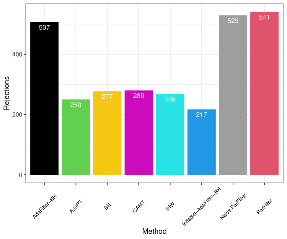
Figure 5.1. Rejection results for $3/[3]$ replicability across the compared methods.

Gene	Stouffer GBHPC $p$-value ($p^{3/[3]}_{i}$)
Mknk2	0.01260681
Mreg	0.01266433
Ecscr	0.01278160
Jarid2	0.01286667
Ncl	0.01313040
Nhsl1	0.01320058
Bcl2l2	0.01328083
Rell1	0.01344367
Fgfbp1	0.01369939
Antxr1	0.01378867
Dkc1	0.01389120
Hspg2	0.01389120
Tnfrsf11a	0.01485068

Table 5.1. Thirteen genes identified as $3/[3]$ replicated by the ParFilter but not by other methods at $q=0.05$.

6. Discussion

In this paper, we introduced the ParFilter (Algorithm 1), a $p$-value-based covariate-adaptive testing procedure for partial conjunction nulls with theoretical finite-sample $\text{FDR}_{\text{rep}}$ control. The procedure is specifically designed to improve power in the power-deprived case of maximum replicability ($u=n$), by drawing on the strategies of filtering and hypothesis weighting. When implemented with the algorithm settings suggested in Sections 3.1—3.5, the procedure demonstrated competitive performance against similar methods in both simulations (Section 4) and a real data case study relating to the immune system (Section 5).

In Appendix A.5, we detail how to extend the ParFilter to identify features whose effects share the same direction (i.e., positive or negative) in at least $u$ of the $n$ studies.

The ParFilter can also be extended to incorporate a post hoc FDR procedure for the base hypotheses. To explain how this is accomplished, consider the following candidate rejection set for testing the base hypotheses $H_{1j},\dots,H_{mj}$:

$$\mathcal{R}_{j}(\tau_{j})\equiv\mathcal{R}(\hat{\mathbf{t}})\cap\{i\in[m]:p_{ij}\leq\tau_{j}\}\subseteq\mathcal{R}(\hat{\mathbf{t}}),$$

where $\tau_{j}\in[0,1]$ is a rejection threshold for the base $p$-values in study $j$. Above, the base null $H_{ij}$ can only be rejected by $\mathcal{R}_{j}(\tau_{j})$ if the PC null $H^{u/[n]}_{i}$ was already rejected by $\mathcal{R}(\hat{\mathbf{t}})$ (i.e., the output of Algorithm 1). Thus, $\mathcal{R}_{j}(\tau_{j})$ provides post hoc inferences by refining the initial inferences made by $\mathcal{R}(\hat{\mathbf{t}})$. Let

$$\text{FDR}_{j}\equiv\text{FDR}_{j}(\tau_{j})=\mathbb{E}\left[\frac{\sum_{i\in\mathcal{R}_{j}(\tau_{j})}I\left\{\text{$H_{ij}$ is true}\right\}}{|\mathcal{R}_{j}(\tau_{j})|\vee 1}\right]$$

denote the false discovery rate associated with the base null hypotheses rejected by $\mathcal{R}_{j}(\tau_{j})$. $\text{FDR}_{j}$ can be controlled by using the post hoc procedure outlined in the theorem below:

Theorem 6.1 (Post hoc FDR control for an individual study).

Suppose the assumptions and conditions of either Theorem 3.3$(i)$ and $(ii)$ all hold. For a given $\text{FDR}_{j}$ target $q_{j}\in(0,1)$, let

$$\hat{\tau}_{j}\equiv\max\left\{\tau_{j}\in\{p_{ij}:i\in[m]\}:\frac{|\mathcal{S}_{k(j)}|\cdot\tau_{j}}{|\mathcal{R}_{j}(\tau_{j})|\vee 1}\leq q_{j}\right\}.$$

Then the post hoc rejection set $\mathcal{R}_{j}(\hat{\tau}_{j})$ has $\text{FDR}_{j}(\hat{\tau}_{j})$ control at level $q_{j}$, i.e., $\text{FDR}_{j}(\hat{\tau}_{j})\leq q_{j}$.

The proof provided in Appendix A.6 is based on Theorem 1 of Katsevich et al., (2023).

A natural direction for future work is to develop more powerful data-driven strategies for constructing $\mathcal{G}_{k}$, $w_{k}$, $\mathbf{u}_{i}$, $\mathcal{S}_{k}$, $p^{u_{ik}/\mathcal{G}_{k}}_{i}$, and $\nu_{ik}$ than those proposed in this paper. In particular, we suspect that $\nu_{ik}$—the local PC weight for feature $i$ in group $k$—may have an optimal construction under data generated from a two-group model (Efron,, 2008), using the results in Sections 3 and 4 of Roquain and van de Wiel, (2008).

Another direction is to convert the ParFilter from a $p$-value-based procedure to an $e$-value-based procedure, similar to how Wang and Ramdas, (2022) converts the BH procedure to an $e$-BH procedure. Interest in $e$-values has grown in recent years as an alternative to $p$-values in hypothesis testing, especially betting-based $e$-values for testing the mean of bounded random variables (Waudby-Smith and Ramdas,, 2023, Orabona and Jun,, 2024). Based on the theoretical underpinnings of the e-BH procedure discussed in Section 5.2 of Wang and Ramdas, (2022), we suspect that an explicit $e$-value version of the ParFilter could offer improved power when the data among the $m$ features within are arbitrarily dependent.

Appendix A Miscellaneous implementational details

A.1. Setting the testing configuration when $u<n$

Generally speaking, one should aim to choose a testing configuration that is balanced for the vast majority of features. In other words, one should avoid choosing a configuration that is unbalanced for most features.

Definition 5 (Imbalance and Balance).

Let $\{\mathcal{G}_{k},w_{k}\}_{k\in[K]}\cup\{\mathbf{u}_{\ell}\}_{\ell\in[m]}$ be a testing configuration for $u/[n]$ replicability, and $i$ be a given $u/[n]$ replicated feature, i.e., the PC null $H^{u/n}_{i}$ is false. Then the testing configuration is said to be:

• imbalanced for feature $i$ if a local PC null $H^{u_{ik}/\mathcal{G}_{k}}_{i}$ is true for some $k\in[K]$.

• balanced for feature $i$ if the local PC null $H^{u_{ik}/\mathcal{G}_{k}}_{i}$ is false for all $k\in[K]$.

To illustrate why minimizing imbalance is important, suppose every $u/[n]$ replicated feature is imbalanced because of a chosen testing configuration. Thus, by Definition 5, let $\mathcal{I}\equiv[m]\backslash\mathcal{H}^{u/[n]}$ be the set of all imbalanced features where $\mathcal{I}$ satisfies

(A.1) $$\mathcal{I}\subseteq\bigcup_{{}_{k\in[K]}}\mathcal{H}_{k}.$$

For a given $\ell\in[K]$, the number of false discoveries made by the ParFilter’s rejection set among the local PC nulls in group $\ell$ is ${|\tiny\widehat{\mathcal{R}}\cap\mathcal{H}_{\ell}|}$, where $\widehat{\mathcal{R}}=\mathcal{R}(\hat{\mathbf{t}})$ is the output of Algorithm 1. Since the ParFilter controls $\text{FDR}_{\ell}(\widehat{\mathcal{R}})$ at level $w_{\ell}\cdot q$, where $q$ is typically small (e.g., $q=0.05$), the number of false discoveries, $|\widehat{\mathcal{R}}\cap\mathcal{H}_{\ell}|$, is generally small. Thus, it follows that $|\widehat{\mathcal{R}}\cap\mathcal{I}|$ is typically small too by (A.1). This means that $\widehat{\mathcal{R}}$ is unlikely to include many $u/[n]$ replicated features, since $\mathcal{I}\equiv[m]\backslash\mathcal{H}^{u/[n]}$.

When $u=n$, one can readily verify that it is impossible to construct a testing configuration that gives rise to imbalanced features; hence, imbalance is not a concern for maximum replicability analyses. Unfortunately, the same cannot be said for the case of $u<n$.

For simplicity, our recommendation for the case of $u<n$ is to set $K=2$ groups, and

(A.2) $$\mathcal{G}_{k}=\{j\in[n]:\text{mod}(j,2)+1\}\quad\text{and}\quad w_{k}=\frac{|\mathcal{G}_{k}|}{n}\quad\text{for each $k\in[2]$},$$

where $\text{mod}(a,b)$ denotes the operation $a$ modulo $b$ for integers $a,b\in\mathbb{N}$.

We recommend constructing the local replicability levels by analyzing the covariates $x_{i1},\dots,x_{in}$ with expert knowledge to predict which base hypotheses among $H_{i1},\dots,H_{in}$ are most likely false, and assigning $\mathbf{u}_{i}\equiv(u_{i1},\dots,u_{iK})$ accordingly, while ensuring the constraints in (3.1) are satisfied. Since our suggestion is rather open-ended, there may be a scenario where $L\in\mathbb{N}$ testing configurations, say

(A.3) $$\{\mathcal{G}^{\ell}_{k},w^{\ell}_{k}\}_{k\in[K_{\ell}]}\cup\{\mathbf{u}^{\ell}_{i}\}\quad\text{ for $\ell\in[L]$},$$

are each considered equally effective in mitigating imbalance. In such scenarios, we recommend choosing a testing configuration for the ParFilter (Algorithm 1) by randomly sampling from (A.3) to hedge against relying too heavily on a single configuration that may not yield powerful results. If the sampling mechanism is independent of $\mathbf{P}$ and $\mathbf{X}$, the $\text{FDR}_{\text{rep}}$ guarantees provided by Theorems 3.3 and 3.4 will still hold:

Theorem A.1 ($\text{FDR}_{\text{rep}}$ control under random testing configurations).

Suppose the $\text{FDR}_{\text{rep}}$ target is $q\in(0,1)$ and (A.3) is a collection of $L\in\mathbb{N}$ candidate testing configurations. Suppose the testing configuration used in the ParFilter (Algorithm 1) is $\{\mathcal{G}^{\ell^{*}}_{k},w^{\ell^{*}}_{k}\}_{k\in[K_{\ell^{*}}]}\cup\{\mathbf{u}^{\ell^{*}}_{i}\}_{i\in[m]}$, where $\ell^{*}\in[L]$ is a random variable that is independent of $\mathbf{P}$ and $\mathbf{X}$. If the assumptions and conditions of either Theorem 3.3 or 3.4 hold, then the ParFilter returns a rejection set $\mathcal{R}(\hat{\mathbf{t}})$ satisfying

$$\text{FDR}_{k}(\mathcal{R}(\hat{\mathbf{t}}))\leq w_{k}\cdot q\;\ \text{ for each }k\in[K]\;\ \text{ and }\;\ \text{FDR}_{\text{rep}}(\mathcal{R}(\hat{\mathbf{t}}))\leq q.$$

Proof.

Let $\mathbb{E}[\text{FDP}_{k}(\hat{\mathbf{t}})|\ell^{*}]$ denote the expected false discovery proportion for group $k$ under a ParFilter implementation that uses $\{\mathcal{G}^{\ell^{*}}_{k},w^{\ell^{*}}_{k}\}_{k\in[K_{\ell^{*}}]}\cup\{\mathbf{u}^{\ell^{*}}_{i}\}_{i\in[m]}$ as the testing configuration. Then $\mathbb{E}[\text{FDP}_{k}(\hat{\mathbf{t}})|\ell^{*}]\leq w_{k}\cdot q$ must hold for each $k\in[K]$ by Theorem 3.3 or 3.4 since $\ell^{*}$ is independent of $\mathbf{P}$ and $\mathbf{X}$. Thus,

$$\text{FDR}_{k}(\mathcal{R}(\hat{\mathbf{t}}))=\mathbb{E}[\text{FDP}_{k}(\hat{\mathbf{t}})]=\mathbb{E}[\mathbb{E}[\text{FDP}_{k}(\hat{\mathbf{t}})|\ell^{*}]]\leq w_{k}\cdot q\quad\text{for each $k\in[K]$}.$$

It then follows from Lemma 3.1 that $\text{FDR}_{\text{rep}}(\mathcal{R}(\hat{\mathbf{t}}))\leq q$. ∎

A.2. Results from the working model in Section 3.4.2

A.2.1. Derivation of $\mathbb{E}[p_{ij}|x_{ij}]$

Under the working model, we have that

$$\mathbb{E}[p_{ij}|x_{ij}] =\int^{1}_{0}p\cdot\left(\pi_{\boldsymbol{\zeta}_{j}}(x_{ij})+(1-\pi_{\boldsymbol{\zeta}_{j}}(x_{ij}))\cdot(1-k_{\boldsymbol{\beta}_{j}}(x_{ij}))\cdot p^{-k_{\boldsymbol{\beta}_{j}}(x_{ij})})\right)\ dp$$

$$=\left[\frac{\left(1-\pi_{\boldsymbol{\zeta}_{j}}(x_{ij})\right)\left(1-k_{\boldsymbol{\beta}_{j}}(x_{ij})\right)p^{2-k_{\boldsymbol{\beta}_{j}}(x_{ij})}}{2-k_{\boldsymbol{\beta}_{j}}(x_{ij})}+\frac{p^{2}\pi_{\boldsymbol{\zeta}_{j}}(x_{ij})}{2}\right]^{1}_{0}$$

$$=\frac{\left(1-\pi_{\boldsymbol{\zeta}_{j}}(x_{ij})\right)\left(1-k_{\boldsymbol{\beta}_{j}}(x_{ij})\right)}{2-k_{\boldsymbol{\beta}_{j}}(x_{ij})}+\frac{\pi_{\boldsymbol{\zeta}_{j}}(x_{ij})}{2}$$

$$=\frac{2\cdot(1-k_{{\boldsymbol{\beta}}_{j}}(x_{ij}))+k_{{\boldsymbol{\beta}}_{j}}(x_{ij})\cdot\pi_{{\boldsymbol{\zeta}}_{j}}(x_{ij})}{4-2\cdot k_{{\boldsymbol{\beta}}_{j}}(x_{ij})}.$$

A.2.2. Derivation of $\omega^{\upsilon/\mathcal{J}}_{i}$ for any $\upsilon\in[u]$ and $\mathcal{J}\subseteq[n]$

First, let $\omega_{ij}\equiv\Pr(\text{$H_{ij}$ is false}|\mathbf{P},\mathbf{X})$ be the probability that $H_{ij}$ is false given $\mathbf{P}$ and $\mathbf{X}$. For convenience, let $\Pr(\text{$H_{ij}$ is false},p_{ij},x_{ij})$ denote the joint density function of $\{\text{$H_{ij}$ is false}\}$, $p_{ij}$, and $x_{ij}$. Moreover, let $\Pr(p_{ij},x_{ij})$ denote the joint density of $(p_{ij},x_{ij})$, and $\Pr(x_{ij})$ denote the density of $x_{ij}$. Then, under the working model,

$$\omega_{ij} =\Pr(\text{$H_{ij}$ is false}|\mathbf{P},\mathbf{X})$$

$$=\Pr(\text{$H_{ij}$ is false}|p_{ij},x_{ij})$$

$$=\frac{\Pr(\text{$H_{ij}$ is false},p_{ij},x_{ij})}{\Pr(p_{ij},x_{ij})}$$

$$=\frac{\Pr(p_{ij}|\text{$H_{ij}$ is false},x_{ij})\Pr(\text{$H_{ij}$ is false}|x_{ij})\Pr(x_{ij})}{\Pr(p_{ij}|x_{ij})\Pr(x_{ij})}$$

$$=\frac{(1-\pi_{\boldsymbol{\zeta}_{j}}(x_{ij}))\cdot f_{\boldsymbol{\beta}_{j}}(p_{ij}|x_{ij})}{f_{\boldsymbol{\zeta}_{j},\boldsymbol{\beta}_{j}}(p_{ij}|x_{ij})}.$$

It follows that

$$\omega^{\upsilon/\mathcal{J}}_{i} =\Pr(\text{$H^{\upsilon/\mathcal{J}}_{i}$ is false}|\mathbf{P},\mathbf{X})$$

$$=\Pr(\text{At least $\upsilon$ null base hypotheses among $H_{ij}$ for $j\in\mathcal{J}$ are false}|\mathbf{P},\mathbf{X})$$

$$=\sum_{\mathcal{L}\subseteq\mathcal{J}:|\mathcal{L}|\geq\upsilon}\prod_{j\in\mathcal{J}\backslash\mathcal{L}}\Pr(\text{$H_{ij}$ is true}|\mathbf{P},\mathbf{X})\prod_{j\in\mathcal{L}}\Pr(\text{$H_{ij}$ is false}|\mathbf{P},\mathbf{X})$$

$$=\sum_{\mathcal{L}\subseteq\mathcal{J}:|\mathcal{L}|\geq\upsilon}\prod_{j\in\mathcal{J}\backslash\mathcal{L}}\Pr(\text{$H_{ij}$ is true}|p_{ij},x_{ij})\prod_{j\in\mathcal{L}}\Pr(\text{$H_{ij}$ is false}|p_{ij},x_{ij})$$

$$=\sum_{\mathcal{L}\subseteq\mathcal{J}:|\mathcal{L}|\geq\upsilon}\prod_{j\in\mathcal{J}\backslash\mathcal{L}}(1-\omega_{ij})\prod_{j\in\mathcal{L}}\omega_{ij}.$$

A.3. Computing the optimal threshold $\hat{\mathbf{t}}$

Data:

  $m\times n$ matrix of base $p$-values $\mathbf{P}$;

  $m\times n$ matrix of covariates $\mathbf{X}$.

Input:

   $\mathcal{G}_{k},w_{k},\mathbf{u}_{i},\lambda_{k},f_{\mathcal{S}_{k}},f_{\boldsymbol{\nu}_{k}},f_{\hat{\pi}_{k}},f_{ik}$ for $k\in[K]$ and $i\in[m]$;

  $\text{FDR}_{\text{rep}}$ target $q\in(0,1)$.

1

2Set $s=1$ and let $\mathbf{t}^{(0)}=(t^{(0)}_{1},\dots,t^{(0)}_{K})=(\infty,\dots,\infty)$.

3For $k=1,\dots,K$, let $\mathbf{t}^{(s)}\equiv(t^{(s)}_{1},\dots,t^{(s)}_{K})$ and define

$$t^{(s)}_{k}\leftarrow\max\Big{\{}t_{k}\in[0,\infty):\widehat{\text{FDP}}_{k}\left((\mathbf{t}^{(s)}_{[1:(k-1)]},t_{k},\mathbf{t}^{(s-1)}_{[(k+1):K]})\right)\leq w_{k}\cdot q\Big{\}}.$$

If $\mathbf{t}^{(s)}=\mathbf{t}^{(s-1)}$, where the equality is understood to hold element-wise, move to the output step. Otherwise, let $s\leftarrow s+1$ and go back to Step 2.

Output: $\hat{\mathbf{t}}=\mathbf{t}^{(s)}.$

Algorithm 2 Computing the optimal vector of thresholds $\hat{\mathbf{t}}$

Algorithm 2 can be used to compute the optimal threshold $\hat{\mathbf{t}}$ implied by Proposition 3.2. Its correctness can be justified by the following proposition.

Proposition A.2 (Correctness of Algorithm 2).

The output of Algorithm 2, is the optimal vector of thresholds in $\mathcal{T}$ as defined in Proposition 3.2.

Proof of Proposition A.2.

The following proof borrows similar induction arguments made in Section 7.2 of Ramdas et al., (2019). Since $\mathbf{t}^{(0)}=(\infty,\dots,\infty)$ upon initialization, we have at time $s=0$ that

(A.4) $$\hat{\mathbf{t}}^{(0)}\succcurlyeq\hat{\mathbf{t}}=(\hat{t}_{1},\dots,\hat{t}_{K}).$$

In what is to follow, we will use induction to prove that

$$\hat{\mathbf{t}}^{(s)}=(\hat{t}^{(s)}_{1},\dots,\hat{t}^{(s)}_{K})\succcurlyeq\hat{\mathbf{t}}$$

for every time iteration $s\geq 0$ with (A.4) being the initial case. Suppose the following inductive assumption is true for any $k\in[K]$:

(A.5) $$(\hat{\mathbf{t}}^{(s)}_{[1:(k-1)]},\hat{t}^{(s-1)}_{k},\hat{\mathbf{t}}^{(s-1)}_{[(k+1):K]})\succcurlyeq\hat{\mathbf{t}}.$$

Since $\hat{t}_{k}\in[0,\infty)$ is the $k$th element of $\hat{\mathbf{t}}$, the inductive assumption above implies the following inequality:

(A.6) $$(\hat{\mathbf{t}}^{(s)}_{[1:(k-1)]},\hat{t}_{k},\hat{\mathbf{t}}^{(s-1)}_{[(k+1):K]})\succcurlyeq\hat{\mathbf{t}}.$$

Since $\hat{\mathbf{t}}\in\mathcal{T}$ by Proposition 3.2, it follows by Definition 4 that

$$w_{k}\cdot q \geq\widehat{\text{FDP}}_{k}\left(\hat{\mathbf{t}}\right)$$

$$=\frac{|\mathcal{S}_{k}|\cdot\hat{\pi}_{k}\cdot\hat{t}_{k}}{|\mathcal{R}\left(\hat{\mathbf{t}}\right)|\vee 1}$$

$$\overset{\tiny(a)}{\geq}\frac{|\mathcal{S}_{k}|\cdot\hat{\pi}_{k}\cdot\hat{t}_{k}}{\left|\mathcal{R}\left((\hat{\mathbf{t}}^{(s)}_{[1:(k-1)]},\hat{t}_{k},\hat{\mathbf{t}}^{(s-1)}_{[(k+1):K]})\right)\right|\vee 1}$$

(A.7) $$=\widehat{\text{FDP}}_{k}\left((\hat{\mathbf{t}}^{(s)}_{[1:(k-1)]},\hat{t}_{k},\hat{\mathbf{t}}^{(s-1)}_{[(k+1):K]})\right)$$

where (a) is consequence of Lemma B.1 and (A.6). Result (A.7) implies that $\hat{t}^{(s)}_{k}\geq\hat{t}_{k}$ because Step 2 of Algorithm 2 computes $\hat{t}^{(s)}_{k}$ to be

$$\hat{t}^{(s)}_{k}= \max\left\{t_{k}\in[0,\infty):\widehat{\text{FDP}}_{k}((\hat{\mathbf{t}}^{(s)}_{[1:(k-1)]},t_{k},\hat{\mathbf{t}}^{(s-1)}_{[(k+1):K]}))\leq w_{k}\cdot q\right\}.$$

Since $\hat{t}^{(s)}_{k}\geq\hat{t}_{k}$, it follows from (A.6) that

(A.8) $$(\hat{\mathbf{t}}^{(s)}_{[1:k]},\hat{\mathbf{t}}^{(s-1)}_{[(k+1):K]})\succcurlyeq\hat{\mathbf{t}}$$

for any $k\in[K]$. Since (A.8) holds by inductive assumption (A.5), it follows that $\hat{\mathbf{t}}^{(s)}\succcurlyeq\hat{\mathbf{t}}$ will be true after executing Step 2 if $\hat{\mathbf{t}}^{(s-1)}\succcurlyeq\hat{\mathbf{t}}$ is true before executing Step 2. Thus, it follows by induction from the initial case (A.4) that

$$\hat{\mathbf{t}}^{(s)}\succcurlyeq\hat{\mathbf{t}}$$

for any time iteration $s\geq 0$ as we have claimed.

To complete the proof, note that it holds by the construction of Step 2 that

(A.9) $$\widehat{\text{FDP}}_{k}\left((\hat{\mathbf{t}}^{(s)}_{[1:k]},\hat{\mathbf{t}}^{(s-1)}_{[(k+1):K]})\right)\leq w_{k}\cdot q$$

for all $k\in[K]$. If $\hat{\mathbf{t}}^{(s^{*}-1)}=\hat{\mathbf{t}}^{(s^{*})}$ holds for some time iteration $s^{*}$, then (A.9) implies that

$$w_{k}\cdot q \geq\widehat{\text{FDP}}_{k}\left((\hat{\mathbf{t}}^{(s^{*})}_{[1:k]},\hat{\mathbf{t}}^{(s^{*}-1)}_{[(k+1):K]})\right)$$

$$=\widehat{\text{FDP}}_{k}\left((\hat{\mathbf{t}}^{(s^{*})}_{[1:k]},\hat{\mathbf{t}}^{(s^{*})}_{[(k+1):K]})\right)$$

(A.10) $$=\widehat{\text{FDP}}_{k}\left(\hat{\mathbf{t}}^{(s^{*})}\right)\text{ for all $k\in[K]$. }$$

It follows from (A.10) and Definition 4 that

(A.11) $$\hat{\mathbf{t}}^{(s^{*})}\in\mathcal{T}.$$

Since $\hat{\mathbf{t}}^{(s)}\succcurlyeq\hat{\mathbf{t}}$ for any time iteration $s\geq 0$ and $\hat{\mathbf{t}}$ is the largest element-wise vector in $\mathcal{T}$ (Proposition 3.2), it follows from (A.11) that $\hat{\mathbf{t}}^{(s^{*})}=\hat{\mathbf{t}}$. ∎

A.4. The ParFilter as a generalization of Bogomolov and Heller, (2018)’s two procedures

For a replicability analysis where $n=2$ and $u=2$, we will show that the ParFilter, under specific algorithm settings, and the adaptive procedure by Bogomolov and Heller, (2018, Section 4.2) are equivalent. The equivalence between the ParFilter and the non-adaptive procedure by Bogomolov and Heller, (2018, Section 3.2) can be shown in a similar fashion, and so, we omit it for brevity.

Let the number of groups be $K=2$, the groups be $\mathcal{G}_{1}=\{1\}$ and $\mathcal{G}_{2}=\{2\}$, and the local replicability levels be $u_{i1}=u_{i2}=1$ and the local PC weights be $\nu_{i1}=\nu_{i2}=1$ for each $i\in[m]$. Moreover, let the weighted null proportion estimator $\hat{\pi}_{k}$ be in the form of (3.19) for each $k\in[2]$ and let the local PC $p$-values be defined as

$$p^{u_{i1}/\mathcal{G}_{1}}_{i}=p^{1/\{1\}}_{i}=p_{i1}\quad\text{and}\quad p^{u_{i2}/\mathcal{G}_{2}}_{i}=p^{1/\{2\}}_{i}=p_{i2}\quad\text{for each $i\in[m]$}.$$

Using the suggestion in Example 3.2, let the selected features be taken as

$$\mathcal{S}_{1}=\{i\in[m]:p_{i2}\leq(w_{2}\cdot q)\wedge\lambda_{2}\}\quad\text{and}\quad\mathcal{S}_{2}=\{i\in[m]:p_{i1}\leq(w_{1}\cdot q)\wedge\lambda_{1}\},$$

respectively. Under the aforementioned ParFilter settings, Algorithm 1 returns the following rejection set:

$$\mathcal{R}(\hat{\mathbf{t}}) =\{i\in\mathcal{S}_{1}:p_{i1}\leq\hat{t}_{1}\wedge\lambda_{1}\}\cap\{i\in\mathcal{S}_{2}:p_{i2}\leq\hat{t}_{2}\wedge\lambda_{2}\}$$

(A.12) $$=\{i\in\mathcal{S}_{1}\cap\mathcal{S}_{2}:(p_{i1},p_{i2})\preccurlyeq(\hat{t}_{1}\wedge\lambda_{1},\hat{t}_{2}\wedge\lambda_{2})\}$$

where $\hat{\mathbf{t}}=(\hat{t}_{1},\hat{t}_{2})$ is the optimal vector of thresholds implied by Proposition 3.2. The adaptive procedure by Bogomolov and Heller, (2018, Section 4.2), under selected features $\mathcal{S}_{1}$ and $\mathcal{S}_{2}$ for group 1 and 2 respectively, yields a rejection set of the form:

(A.13) $$\tilde{\mathcal{R}}\equiv\left\{\ell\in\mathcal{S}_{1}\cap\mathcal{S}_{2}:(p_{\ell 1},p_{\ell 2})\preccurlyeq\left(\frac{R\cdot w_{1}\cdot q}{|\mathcal{S}_{1}|\cdot\hat{\pi}_{1}}\wedge\lambda_{1},\frac{R\cdot w_{2}\cdot q}{|\mathcal{S}_{2}|\cdot\hat{\pi}_{2}}\wedge\lambda_{2}\right)\right\}$$

where

(A.14) $$R\equiv\max\left\{r:\sum_{\ell\in\mathcal{S}_{1}\cap\mathcal{S}_{2}}I\left\{(p_{\ell 1},p_{\ell 2})\preccurlyeq\left(\frac{r\cdot w_{1}\cdot q}{|\mathcal{S}_{1}|\cdot\hat{\pi}_{1}}\wedge\lambda_{1},\frac{r\cdot w_{2}\cdot q}{|\mathcal{S}_{2}|\cdot\hat{\pi}_{2}}\wedge\lambda_{2}\right)\right\}=r\right\}.$$

If $R$ does not exist, then $\tilde{\mathcal{R}}$ is defined to be an empty set. To complete this proof, we will show that $\tilde{\mathcal{R}}=\mathcal{R}(\hat{\mathbf{t}})$ by proving the following two inclusions:

(A.15) $$\tilde{\mathcal{R}}\subseteq\mathcal{R}(\hat{\mathbf{t}})\quad\text{and}\quad\mathcal{R}(\hat{\mathbf{t}})\subseteq\tilde{\mathcal{R}}.$$

Assume $\tilde{\mathcal{R}}$ is non-empty and let $\tilde{\mathbf{t}}=(\tilde{t}_{1},\tilde{t}_{2})$ where

(A.16) $$\tilde{t}_{1}=\frac{R\cdot w_{1}\cdot q}{|\mathcal{S}_{1}|\cdot\hat{\pi}_{1}}\quad\text{ and }\quad\tilde{t}_{2}=\frac{R\cdot w_{2}\cdot q}{|\mathcal{S}_{2}|\cdot\hat{\pi}_{2}}.$$

It follows from (A.13) and the form of the ParFilter’s rejection set given in (A.12) that

$$\tilde{\mathcal{R}}=\left\{i\in\mathcal{S}_{1}\cap\mathcal{S}_{1}:(p_{i1},p_{i2})\preccurlyeq\left(\tilde{t}_{1}\wedge\lambda_{1},\tilde{t}_{2}\wedge\lambda_{2}\right)\right\}=\mathcal{R}(\tilde{\mathbf{t}}).$$

Since $R=|\tilde{\mathcal{R}}|$ by (A.14), it follows from the relationship above and (A.16) that

$$\tilde{t}_{1}=\frac{|\mathcal{R}(\tilde{\mathbf{t}})|\cdot w_{1}\cdot q}{|\mathcal{S}_{1}|\cdot\hat{\pi}_{1}}\quad\text{ and }\quad\tilde{t}_{2}=\frac{|\mathcal{R}(\tilde{\mathbf{t}})|\cdot w_{2}\cdot q}{|\mathcal{S}_{2}|\cdot\hat{\pi}_{2}}.$$

The equalities above can be rearranged to yield

$$\widehat{\text{FDP}}_{1}(\tilde{\mathbf{t}})\equiv\frac{|\mathcal{S}_{1}|\cdot\hat{\pi}_{1}\cdot\tilde{t}_{1}}{|\mathcal{R}(\tilde{\mathbf{t}})|}=w_{1}\cdot q\quad\text{ and }\quad\widehat{\text{FDP}}_{2}(\tilde{\mathbf{t}})\equiv\frac{|\mathcal{S}_{2}|\cdot\hat{\pi}_{2}\cdot\tilde{t}_{2}}{|\mathcal{R}(\tilde{\mathbf{t}})|}=w_{2}\cdot q,$$

which implies that $\tilde{\mathbf{t}}\in\mathcal{T}$ by Definition 4. Since $\hat{\mathbf{t}}$ is the largest element-wise vector in $\mathcal{T}$ by Proposition 3.2, it must be the case that $\hat{\mathbf{t}}\succcurlyeq\tilde{\mathbf{t}}$. Hence, it follows from Lemma B.1 and $\hat{\mathbf{t}}\succcurlyeq\tilde{\mathbf{t}}$ that

$$\tilde{\mathcal{R}}=\mathcal{R}(\tilde{\mathbf{t}})\subseteq\mathcal{R}(\hat{\mathbf{t}}),$$

which proves the left inclusion of (A.15). We will now prove the right inclusion of (A.15), i.e., $\mathcal{R}(\hat{\mathbf{t}})\subseteq\tilde{\mathcal{R}}$.

Assume $\mathcal{R}(\hat{\mathbf{t}})$ is non-empty. We have that

$$\sum_{i\in\mathcal{S}_{1}\cap\mathcal{S}_{2}} I\left\{(p_{i1},p_{i2})\preccurlyeq\left(\frac{|\mathcal{R}(\hat{\mathbf{t}})|\cdot w_{1}\cdot q}{|\mathcal{S}_{1}|\cdot\hat{\pi}_{1}}\wedge\lambda_{1},\frac{|\mathcal{R}(\hat{\mathbf{t}})|\cdot w_{2}\cdot q}{|\mathcal{S}_{2}|\cdot\hat{\pi}_{2}}\wedge\lambda_{2}\right)\right\}$$

$$\overset{\tiny(a)}{=}\sum_{i\in\mathcal{S}_{1}\cap\mathcal{S}_{2}}I\left\{(p_{i1},p_{i2})\preccurlyeq(\hat{t}_{1}\wedge\lambda_{1},\hat{t}_{2}\wedge\lambda_{2})\right\}$$

$$=\left|\{i\in\mathcal{S}_{1}\cap\mathcal{S}_{2}:(p_{i1},p_{i2})\preccurlyeq(\hat{t}_{1}\wedge\lambda_{1},\hat{t}_{2}\wedge\lambda_{2})\}\right|$$

$$\overset{\tiny(b)}{=}|\mathcal{R}(\hat{\mathbf{t}})|$$

where $(a)$ is a result of Lemma B.3 and $(b)$ is a result (A.12). By the definition of $R$ in (A.14), it must follow from the display above that

(A.17) $$R\geq|\mathcal{R}(\hat{\mathbf{t}})|.$$

Hence,

$$\mathcal{R}(\hat{\mathbf{t}}) =\left\{i\in\mathcal{S}_{1}\cap\mathcal{S}_{2}:(p_{i1},p_{i2})\preccurlyeq\left(\hat{t}_{1}\wedge\lambda_{1},\hat{t}_{2}\wedge\lambda_{2}\right)\right\}$$

$$\overset{\tiny(c)}{=}\left\{i\in\mathcal{S}_{1}\cap\mathcal{S}_{2}:(p_{i1},p_{i2})\preccurlyeq\left(\frac{|\mathcal{R}(\hat{\mathbf{t}})|\cdot w_{1}\cdot q}{|\mathcal{S}_{1}|\cdot\hat{\pi}_{1}}\wedge\lambda_{1},\frac{|\mathcal{R}(\hat{\mathbf{t}})|\cdot w_{2}\cdot q}{|\mathcal{S}_{2}|\cdot\hat{\pi}_{2}}\wedge\lambda_{2}\right)\right\}$$

$$\overset{\tiny(d)}{\subseteq}\left\{i\in\mathcal{S}_{1}\cap\mathcal{S}_{2}:(p_{i1},p_{i2})\preccurlyeq\left(\frac{R\cdot w_{1}\cdot q}{|\mathcal{S}_{1}|\cdot\hat{\pi}_{1}}\wedge\lambda_{1},\frac{R\cdot w_{2}\cdot q}{|\mathcal{S}_{2}|\cdot\hat{\pi}_{2}}\wedge\lambda_{2}\right)\right\}$$

$$=\tilde{\mathcal{R}}$$

where $(c)$ is a result of Lemma B.3 and $(d)$ is a result of (A.17). Thus, $\mathcal{R}(\hat{\mathbf{t}})\subseteq\tilde{\mathcal{R}}$.

A.5. Directional inference with the ParFilter

In replicability analysis, it may be valuable to identify features that exhibit the same direction of effect in at least $u$ out of $n$ studies. We refer to this as a directional replicability analysis. To develop a methodology for conducting such an analysis, we first define the left-sided and right-sided base null hypotheses as

$$\text{$H^{-}_{ij}:\mu_{ij}\geq 0\quad$ and $\quad H^{+}_{ij}:\mu_{ij}\leq 0\quad$ respectively for each $(i,j)\in[m]\times[n]$}.$$

Define the left-sided and right-sided PC null hypotheses as

$$H^{-u/[n]}_{i}: |\{j\in[n]:\mu_{ij}\geq 0\}|\geq n-u+1\quad\text{and}$$

$$\quad\quad H^{+u/[n]}_{i}:|\{j\in[n]:\mu_{ij}\leq 0\}|\geq n-u+1\quad\text{respectively for each $i\in[m]$.}$$

Above, rejecting $H^{-u/[n]}_{i}$ is a declaration that feature $i$ has a negative effect in at least $u$ of the $n$ studies. Likewise, rejecting $H^{+u/[n]}_{i}$ is a declaration that that feature $i$ has a positive effect in at least $u$ of the $n$ studies. Let the set of true left-sided and right-sided PC nulls be

$$\mathcal{H}^{-u/[n]}\equiv\{i\in[m]:\text{$H^{-u/[n]}_{i}$ is true}\}\quad\text{and}\quad\mathcal{H}^{+u/[n]}\equiv\{i\in[m]:\text{$H^{+u/[n]}_{i}$ is true}\}$$

respectively. If the conditions of either Theorem 3.3 or 3.4 are met, the ParFilter can be used to perform a directional replicability analysis by carrying out the following two steps:

1. Create a rejection set $\widehat{\mathcal{R}}^{-}$ for the left-sided PC nulls that controls the left-sided $\text{FDR}_{\text{rep}}$,

   $$\mathbb{E}\left[\frac{\sum_{i\in\mathcal{H}^{-u/[n]}}I\{i\in\widehat{\mathcal{R}}^{-}\}}{|\widehat{\mathcal{R}}^{-}|\vee 1}\right],$$

   at level $q/2$ for some $q\in(0,1)$; and

2. Create a rejection set $\widehat{\mathcal{R}}^{+}$ for the right-sided PC nulls that controls the right-sided $\text{FDR}_{\text{rep}}$,

   $$\mathbb{E}\left[\frac{\sum_{i\in\mathcal{H}^{+u/[n]}}I\{i\in\widehat{\mathcal{R}}^{+}\}}{|\widehat{\mathcal{R}}^{+}|\vee 1}\right],$$

   at level $q/2$.

By design, $\widehat{\mathcal{R}}^{-}$ and $\widehat{\mathcal{R}}^{+}$ together will provide $\text{FDR}^{\pm}_{\text{rep}}$ control at level $q$, where

$$\text{FDR}^{\pm}_{\text{rep}}\equiv\mathbb{E}\left[\frac{\sum_{i\in\mathcal{H}^{-u/[n]}}I\{i\in\widehat{\mathcal{R}}^{-}\}+\sum_{i\in\mathcal{H}^{+u/[n]}}I\{i\in\widehat{\mathcal{R}}^{+}\}}{|\widehat{\mathcal{R}}^{-}\cup\widehat{\mathcal{R}}^{+}|\vee 1}\right].$$

In words, $\text{FDR}^{\pm}_{\text{rep}}$ is the expected number of features falsely identified as having at least $u$ effects in the left direction by $\widehat{\mathcal{R}}^{-}$ and in the right direction by $\widehat{\mathcal{R}}^{+}$, out of the total number of features in $\widehat{\mathcal{R}}^{-}\cup\widehat{\mathcal{R}}^{+}$. The justification for $\text{FDR}^{+/-}_{\text{rep}}$ control at level $q$ is as follows:

$$\text{FDR}^{\pm}_{\text{rep}} =\mathbb{E}\left[\frac{\sum_{i\in\mathcal{H}^{-u/[n]}}I\{i\in\widehat{\mathcal{R}}^{-}\}}{|\widehat{\mathcal{R}}^{-}\cup\widehat{\mathcal{R}}^{+}|\vee 1}\right]+\mathbb{E}\left[\frac{\sum_{i\in\mathcal{H}^{+u/[n]}}I\{i\in\widehat{\mathcal{R}}^{+}\}}{|\widehat{\mathcal{R}}^{-}\cup\widehat{\mathcal{R}}^{+}|\vee 1}\right]$$

$$\leq\mathbb{E}\left[\frac{\sum_{i\in\mathcal{H}^{-u/[n]}}I\{i\in\widehat{\mathcal{R}}^{-}\}}{|\widehat{\mathcal{R}}^{-}|\vee 1}\right]+\mathbb{E}\left[\frac{\sum_{i\in\mathcal{H}^{+u/[n]}}I\{i\in\widehat{\mathcal{R}}^{+}\}}{|\widehat{\mathcal{R}}^{+}|\vee 1}\right]$$

$$\overset{\tiny(a)}{\leq}\frac{q}{2}+\frac{q}{2}$$

$$=q$$

where (a) is a result of $\widehat{\mathcal{R}}^{-}$ and $\widehat{\mathcal{R}}^{+}$ having left and right-sided $\text{FDR}_{\text{rep}}$ control at level $q/2$, respectively.

A.6. Proof of Theorem 6.1 (Post hoc FDR control for individual studies)

.

First, note that

$$\mathcal{R}_{j}(\hat{\tau}_{j})\equiv\mathcal{R}(\hat{\mathbf{t}})\cap\{i\in[m]:p_{ij}\leq\hat{\tau}_{j}\}\overset{\tiny(a)}{=}\mathcal{R}(\hat{\mathbf{t}})\cap\{i\in\mathcal{S}_{k(j)}:p_{ij}\leq\hat{\tau}_{j}\}$$

where $k(j)$ is the group where study $j$ belongs, i.e., $j\in\mathcal{G}_{k(j)}$. Equality $(a)$ above follows from the fact that $\mathcal{R}(\hat{\mathbf{t}})\subseteq\mathcal{S}_{k}$ for any group $k$ by (3.6). We also note that conditioning on $\{\mathbf{P}_{\cdot\mathcal{G}_{k(j)}},\mathbf{X}\}$ fixes $\mathcal{S}_{k(j)}$ by Condition 1.

$\mathcal{R}_{j}(\hat{\tau}_{j})=\mathcal{R}(\hat{\mathbf{t}})\cap\{i\in\mathcal{S}_{k(j)}:p_{ij}\leq\hat{\tau}_{j}\}$ can be interpreted as the output of the Focused BH procedure by Katsevich et al., (2023, Procedure 1) for simultaneously testing

$H_{ij}$ for $i\in\mathcal{S}_{k(j)}$,

where $\hat{\tau}_{j}$ is equivalent to their equation $(6)$ and $\mathcal{R}(\hat{\mathbf{t}})$ is what they call a screening function. By Lemma B.4 in Appendix B, $\mathcal{R}(\hat{\mathbf{t}})$ is a stable screening function according to Theorem 1$(ii)$ of Katsevich et al., (2023) when $\mathbf{X}$ is given. Thus, by Theorem 1 of Katsevich et al., (2023), it holds that

$$\mathbb{E}\left[\frac{\sum_{i\in\mathcal{R}_{j}(\hat{\tau}_{j})}I\{\text{$H_{ij}$ is true}\}}{|\mathcal{R}_{j}(\hat{\tau}_{j})|\vee 1}\Bigg{|}\mathbf{P}_{\cdot\mathcal{G}_{k(j)}},\mathbf{X}\right]\leq q_{j}.$$

By the double expectation property, it follows that $\text{FDR}_{j}(\hat{\tau}_{j})\leq q_{j}$. ∎

Appendix B Technical lemmas

B.1. Lemmas regarding properties of the rejection sets

This section states and proves technical lemmas used in the proof of Proposition A.2 in Appendix A.3, the proof that the ParFilter generalizes Bogomolov and Heller, (2018)’s procedures in Appendix A.4, and the proofs of Propositions 3.2, Theorems 3.3, and 3.4 in Appendix C. These technical results all concern properties of the rejection set $\mathcal{R}(\hat{\mathbf{t}})$ defined in (3.6).

Hereafter, we will occasionally use

$\mathcal{R}(\mathbf{t})=\mathcal{R}(\mathbf{t};\mathbf{P},\mathbf{X})$, $\quad\mathcal{T}=\mathcal{T}(\mathbf{P};\mathbf{X})$, and $\quad\widehat{\text{FDP}}_{k}(\mathbf{t})=\widehat{\text{FDP}}_{k}(\mathbf{t};\mathbf{P},\mathbf{X})$

to emphasize that $\mathcal{R}(\mathbf{t})$, $\mathcal{T}$, and $\widehat{\text{FDP}}_{k}(\mathbf{t})$ also depend on the base $p$-values $\mathbf{P}$ and covariates $\mathbf{X}$.

B.1.1. Comparison of rejection sets

Lemma B.1 ($\mathcal{R}(\mathbf{t}^{\prime\prime})\subseteq\mathcal{R}(\mathbf{t}^{\prime})$ for $\mathbf{t}^{\prime}\succcurlyeq\mathbf{t}^{\prime\prime}$).

Let $\mathbf{t}^{\prime},\mathbf{t}^{\prime\prime}\in[0,\infty)^{K}$ be vectors that satisfy $\mathbf{t}^{\prime}\succcurlyeq\mathbf{t}^{\prime\prime}$. Then $\mathcal{R}(\mathbf{t}^{\prime\prime})\subseteq\mathcal{R}(\mathbf{t}^{\prime})$.

Proof of Lemma B.1.

Write $\mathbf{t}^{\prime}=(t^{\prime}_{1},\dots,t^{\prime}_{K})$ and $\mathbf{t}^{\prime\prime}=(t^{\prime\prime}_{1},\dots,t^{\prime\prime}_{K})\in[0,\infty)^{K}$. Since $\mathbf{t}^{\prime}\succcurlyeq\mathbf{t}^{\prime\prime}$, it follows that

$$\left\{i\in\mathcal{S}_{k}:p^{u_{ik}/\mathcal{G}_{k}}_{i}\leq\nu_{ik}\cdot t^{\prime\prime}_{k}\right\}\subseteq\left\{i\in\mathcal{S}_{k}:p^{u_{ik}/\mathcal{G}_{k}}_{i}\leq\nu_{ik}\cdot t^{\prime}_{k}\right\}$$

for each $k\in[K]$. Thus,

$$\mathcal{R}(\mathbf{t}^{\prime\prime}) =\bigcap_{k\in[K]}\left\{i\in\mathcal{S}_{k}:p^{u_{ik}/\mathcal{G}_{k}}_{i}\leq(\nu_{ik}\cdot t^{\prime\prime}_{k})\wedge\lambda_{k}\right\}$$

$$=\bigcap_{k\in[K]}\left(\left\{i\in\mathcal{S}_{k}:p^{u_{ik}/\mathcal{G}_{k}}_{i}\leq\nu_{ik}\cdot t^{\prime\prime}_{k}\right\}\cap\left\{i\in\mathcal{S}_{k}:p^{u_{ik}/\mathcal{G}_{k}}_{i}\leq\lambda_{k}\right\}\right)$$

$$\subseteq\bigcap_{k\in[K]}\left(\left\{i\in\mathcal{S}_{k}:p^{u_{ik}/\mathcal{G}_{k}}_{i}\leq\nu_{ik}\cdot t^{\prime}_{k}\right\}\cap\left\{i\in\mathcal{S}_{k}:p^{u_{ik}/\mathcal{G}_{k}}_{i}\leq\lambda_{k}\right\}\right)$$

$$=\bigcap_{k\in[K]}\left\{i\in\mathcal{S}_{k}:p^{u_{ik}/\mathcal{G}_{k}}_{i}\leq(\nu_{ik}\cdot t^{\prime}_{k})\wedge\lambda_{k}\right\}$$

$$=\mathcal{R}(\mathbf{t}^{\prime}).$$

∎

B.1.2. Self-consistency of rejection sets

The following lemma shows that $\mathcal{R}(\hat{\mathbf{t}})$ satisfies a property akin to the self-consistency condition described in Definition 2.5 of Blanchard and Roquain, (2008).

Lemma B.2 (Self-consistency).

Let $\mathcal{R}(\hat{\mathbf{t}})$ be the rejection set output of Algorithm 1 where $\hat{\mathbf{t}}$ is the optimal vector of thresholds in $\mathcal{T}$ (Proposition 3.2). If the selected features for group $k$, i.e., $\mathcal{S}_{k}\subseteq[m]$, is non-empty, then it holds that

(B.1) $$I\left\{i\in\mathcal{R}(\hat{\mathbf{t}})\right\}\leq I\left\{p^{u_{ik}/\mathcal{G}_{k}}_{i}\leq\frac{\nu_{ik}\cdot|\mathcal{R}(\hat{\mathbf{t}})|\cdot w_{k}\cdot q}{|\mathcal{S}_{k}|\cdot\hat{\pi}_{k}}\right\}\quad\text{for any $i\in[m]$.}$$

Proof of Lemma B.2.

If $\mathcal{R}(\hat{\mathbf{t}})$ is empty, then $I\left\{i\in\mathcal{R}(\hat{\mathbf{t}})\right\}=0$ and

$$I\left\{p^{u_{ik}/\mathcal{G}_{k}}_{i}\leq\frac{\nu_{ik}\cdot|\mathcal{R}(\hat{\mathbf{t}})|\cdot w_{k}\cdot q}{|\mathcal{S}_{k}|\cdot\hat{\pi}_{k}}\right\}=I\left\{p^{u_{ik}/\mathcal{G}_{k}}_{i}\leq 0\right\}\geq 0\quad\text{for each $i\in[m]$.}$$

Thus, (B.1) holds true in this case.
 
Now consider the case where $\mathcal{R}(\hat{\mathbf{t}})$ is non-empty. Since $\hat{\mathbf{t}}\in\mathcal{T}$ by Proposition 3.2, it follows by Definition 4 that

$$\widehat{\text{FDP}}_{k}(\hat{\mathbf{t}})\leq w_{k}\cdot q.$$

Rearranging the aforementioned inequality yields

(B.2) $$\hat{t}_{k} \leq\frac{|\mathcal{R}(\hat{\mathbf{t}})|\cdot w_{k}\cdot q}{|\mathcal{S}_{k}|\cdot\hat{\pi}_{k}}.$$

Since $\mathcal{R}(\hat{\mathbf{t}})\subseteq\{\ell\in\mathcal{S}_{k}:p^{u_{\ell k}/\mathcal{G}_{k}}_{\ell}\leq\nu_{\ell k}\cdot\hat{t}_{k}\}$, it follows from (B.2) that

$$i\in\mathcal{R}(\hat{\mathbf{t}})\implies p^{u_{ik}/\mathcal{G}_{k}}_{i}\leq\nu_{ik}\cdot\frac{|\mathcal{R}(\hat{\mathbf{t}})|\cdot w_{k}\cdot q}{|\mathcal{S}_{k}|\cdot\hat{\pi}_{k}}.$$

The direction of the implication above gives the inequality displayed in (B.1). ∎

B.1.3. The rejection thresholds $\hat{\mathbf{t}}$ as a function of $\mathcal{R}(\hat{\mathbf{t}})$

Lemma B.3.

Let $\mathcal{R}(\hat{\mathbf{t}})$ be the output of Algorithm 1 where $\hat{\mathbf{t}}$ is the optimal vector of thresholds in $\mathcal{T}$ (Proposition 3.2). If $\mathcal{R}(\hat{\mathbf{t}})$ is non-empty, then

$$\hat{\mathbf{t}}=(\hat{t}_{1},\dots,\hat{t}_{K})=\left(\frac{|\mathcal{R}(\hat{\mathbf{t}})|\cdot w_{1}\cdot q}{|\mathcal{S}_{1}|\cdot\hat{\pi}_{1}},\dots,\frac{|\mathcal{R}(\hat{\mathbf{t}})|\cdot w_{K}\cdot q}{|\mathcal{S}_{K}|\cdot\hat{\pi}_{K}}\right).$$

Proof of Lemma B.3.

Since $\hat{\mathbf{t}}\in\mathcal{T}$ by Proposition 3.2, we have by Definition 4 that

(B.3) $$\left(\widehat{\text{FDP}}_{1}(\hat{\mathbf{t}}),\dots,\widehat{\text{FDP}}_{K}(\hat{\mathbf{t}})\right)\preccurlyeq(w_{1}\cdot q,\dots,w_{K}\cdot q).$$

Using the definition for $\widehat{\text{FDP}}_{k}$ given in (3.15), rearranging the above relationship when $\mathcal{R}(\hat{\mathbf{t}})$ is non-empty yields

(B.4) $$\underbrace{\left(\frac{|\mathcal{R}(\hat{\mathbf{t}})|\cdot w_{1}\cdot q}{|\mathcal{S}_{1}|\cdot\hat{\pi}_{1}},\dots,\frac{|\mathcal{R}(\hat{\mathbf{t}})|\cdot w_{K}\cdot q}{|\mathcal{S}_{K}|\cdot\hat{\pi}_{K}}\right)}_{\begin{matrix}\equiv\hat{\mathbf{t}}^{*}\end{matrix}}\succcurlyeq(\hat{t}_{1},\dots,\hat{t}_{K})=\hat{\mathbf{t}}.$$

Note that if $\mathcal{R}(\hat{\mathbf{t}})$ is non-empty, then $\mathcal{S}_{k}$ must also be non-empty (i.e., $|\mathcal{S}_{k}|>0$) for each $k\in[K]$. From the inequality in (B.4), we have by Lemma B.1 that

(B.5) $$\mathcal{R}(\hat{\mathbf{t}})\subseteq\mathcal{R}\left(\hat{\mathbf{t}}^{*}\right).$$

Moreover,

$$\widehat{\text{FDP}}_{k}\left(\hat{\mathbf{t}}^{*}\right) =\frac{|\mathcal{S}_{k}|\cdot\hat{\pi}_{k}\cdot\left(\frac{|\mathcal{R}(\hat{\mathbf{t}})|\cdot w_{k}\cdot q}{|\mathcal{S}_{k}|\cdot\hat{\pi}_{k}}\right)}{\left|\mathcal{R}\left(\hat{\mathbf{t}}^{*}\right)\right|\vee 1}$$

$$=\frac{|\mathcal{R}(\hat{\mathbf{t}})|\cdot w_{k}\cdot q}{\left|\mathcal{R}\left(\hat{\mathbf{t}}^{*}\right)\right|\vee 1}$$

$$\overset{\tiny(a)}{\leq}\frac{|\mathcal{R}(\hat{\mathbf{t}})|\cdot w_{k}\cdot q}{|\mathcal{R}(\hat{\mathbf{t}})|\vee 1}$$

$$\leq w_{k}\cdot q\quad\text{ for all $k\in[K]$ }$$

where (a) is a result of (B.5). Hence, it follows from the display above and Definition 4 that

(B.6) $$\hat{\mathbf{t}}^{*}\in\mathcal{T}.$$

Since $\hat{\mathbf{t}}$ is the largest element-wise vector in $\mathcal{T}$ (Proposition 3.2), it follows from (B.4) and (B.6) that $\hat{\mathbf{t}}^{*}=\hat{\mathbf{t}}$, thereby completing the proof. ∎

B.1.4. Stability of the ParFilter’s rejection set

Lemma B.4 (Stability of $\mathcal{R}(\hat{\mathbf{t}})$).

Consider an implementation of the ParFilter (Algorithm 1) where

• $f_{\mathcal{S}_{k}}$ ensures that $\mathcal{S}_{k}$ stable (i.e., Condition 2 is met) for each $k\in[K]$;

• $f_{\boldsymbol{\nu}_{k}}$ ensures that $\boldsymbol{\nu}_{k}$ a function of the base $p$-values in $\mathbf{P}_{(-\mathcal{S}_{k})\mathcal{G}_{k}}$, the covariates $\mathbf{X}$, and the selection set $\mathcal{S}_{k}$ only (i.e., Condition 4$(a)$ is met) for each $k\in[K]$;

• $f_{\hat{\pi}_{k}}$ ensures that $\hat{\pi}_{k}$ is either one or in the form of (3.19) for each $k\in[K]$.

Then the rejection set $\mathcal{R}(\hat{\mathbf{t}})$ outputted by ParFilter is stable, i.e. for any $i\in\mathcal{R}(\hat{\mathbf{t}})$,

fixing $\mathbf{P}_{(-i)\cdot}$ and $\mathbf{X}$, and changing $\mathbf{P}_{i\cdot}$ so that $i\in\mathcal{R}(\hat{\mathbf{t}})$ still holds,

will not change the set $\mathcal{R}(\hat{\mathbf{t}})$.

Proof of Lemma B.4.

The following proof shares similar arguments seen in Katsevich et al., (2023)’s proof of their Theorem 1$(ii)$. Let $\mathbf{P}^{\prime}$ and $\mathbf{P}^{\prime\prime}$ be two $m\times n$ matrices of $p$-values. Let

(B.7) $${p^{\prime}}^{{u}_{\ell k}/\mathcal{G}_{k}}_{\ell}=f_{\ell k}(\mathbf{P}^{\prime}_{\ell\mathcal{G}_{k}};{u}_{\ell k})\quad\text{and}\quad{p^{\prime\prime}}^{u_{\ell k}/\mathcal{G}_{k}}_{\ell}=f_{\ell k}(\mathbf{P}^{\prime\prime}_{\ell\mathcal{G}_{k}};u_{\ell k})$$

denote local PC $p$-values for feature $\ell$ of group $k$, constructed from $(\mathbf{P}^{\prime}_{\ell\mathcal{G}_{k}},u_{\ell k})$ and $(\mathbf{P}^{\prime\prime}_{\ell\mathcal{G}_{k}},u_{\ell k})$ respectively. Let

$$\mathcal{S}^{\prime}_{k}=f_{\mathcal{S}_{k}}(\mathbf{P}^{\prime};\mathbf{X})\quad\text{and}\quad\mathcal{S}^{\prime\prime}_{k}=f_{\mathcal{S}_{k}}(\mathbf{P}^{\prime\prime};\mathbf{X})$$

denote selected features for group $k$, constructed from $(\mathbf{P}^{\prime},\mathbf{X})$ and $(\mathbf{P}^{\prime\prime},\mathbf{X})$ respectively. Let

(B.8) $$\boldsymbol{\nu}^{\prime}_{k}=(\nu^{\prime}_{1k},\dots,\nu^{\prime}_{mk})=f_{\boldsymbol{\nu}_{k}}(\mathbf{P}^{\prime};\mathbf{X})\quad\text{and}\quad\boldsymbol{\nu}^{\prime\prime}=(\nu^{\prime\prime}_{1k},\dots,\nu^{\prime\prime}_{mk})=f_{\boldsymbol{\nu}_{k}}(\mathbf{P}^{\prime\prime};\mathbf{X})$$

denote local PC weights for group $k$, constructed from $(\mathbf{P}^{\prime},\mathbf{X})$ and $(\mathbf{P}^{\prime\prime},\mathbf{X})$ respectively. Let

(B.9) $$\hat{\pi}^{\prime}_{k}=f_{\hat{\pi}_{k}}(\mathbf{P}^{\prime};\mathbf{X},\lambda_{k})\quad\text{ and }\quad\hat{\pi}^{\prime\prime}_{k}=f_{\hat{\pi}_{k}}(\mathbf{P}^{\prime\prime};\mathbf{X},\lambda_{k})$$

denote weighted null proportion estimators for group $k$, constructed from $(\mathbf{P}^{\prime},\mathbf{X},\lambda_{k})$ and $(\mathbf{P}^{\prime\prime},\mathbf{X},\lambda_{k})$ respectively. Let

$$\hat{\mathbf{t}}^{\prime}=(\hat{t}^{\prime}_{1},\dots,\hat{t}^{\prime}_{K})\quad \quad\hat{\mathbf{t}}^{\prime\prime}=(\hat{t}^{\prime\prime}_{1},\dots,\hat{t}^{\prime\prime}_{K})$$ and

be the optimal thresholds implied by Proposition 3.2 in

$$\mathcal{T}(\mathbf{P}^{\prime};\mathbf{X})\quad\text{and}\quad\mathcal{T}(\mathbf{P}^{\prime\prime};\mathbf{X})$$

respectively. By Proposition 3.2, we have that

(B.10) $$\widehat{\text{FDP}}_{k}(\hat{\mathbf{t}}^{\prime};\mathbf{P}^{\prime},\mathbf{X})= \frac{|\mathcal{S}^{\prime}_{k}|\cdot\hat{\pi}^{\prime}_{k}\cdot\hat{t}^{\prime}_{k}}{|\mathcal{R}(\hat{\mathbf{t}}^{\prime};\mathbf{P}^{\prime},\mathbf{X})|\vee 1}\leq w_{k}\cdot q\quad\text{and}$$

(B.11) $$\quad\widehat{\text{FDP}}_{k}(\hat{\mathbf{t}}^{\prime\prime};\mathbf{P}^{\prime\prime},\mathbf{X})=\frac{|\mathcal{S}^{\prime\prime}_{k}|\cdot\hat{\pi}^{\prime\prime}_{k}\cdot\hat{t}^{\prime\prime}_{k}}{|\mathcal{R}(\hat{\mathbf{t}}^{\prime\prime};\mathbf{P}^{\prime\prime},\mathbf{X})|\vee 1}\leq w_{k}\cdot q$$

for each group $k\in[K]$.

We will assume that

(B.12) $$\mathbf{P}^{\prime}_{(-i)\cdot}=\mathbf{P}_{(-i)\cdot}^{\prime\prime},\quad\text{and}\quad i\in\mathcal{R}(\hat{\mathbf{t}}^{\prime};\mathbf{P}^{\prime},\mathbf{X})\cap\mathcal{R}(\hat{\mathbf{t}}^{\prime\prime};\mathbf{P}^{\prime\prime},\mathbf{X})\text{ for a given }i\in[m],$$

i.e. the matrices $\mathbf{P}^{\prime}$ and $\mathbf{P}^{\prime\prime}$ only possibly differ in the $i$-th row in such a way that feature $i$ is still in both of the ParFilter rejection sets based on $(\mathbf{P}^{\prime},\mathbf{X}$) and $(\mathbf{P}^{\prime\prime},\mathbf{X})$. To prove the lemma, it suffices to show under the assumption in (B.12) that

(B.13) $$\mathcal{R}(\hat{\mathbf{t}}^{\prime};\mathbf{P}^{\prime},\mathbf{X})=\mathcal{R}(\hat{\mathbf{t}}^{\prime\prime};\mathbf{P}^{\prime\prime},\mathbf{X}).$$

Since $f_{\mathcal{S}_{k}}$ is a stable selection rule and

(B.14) $$\mathcal{R}(\hat{\mathbf{t}}^{\prime};\mathbf{P}^{\prime},\mathbf{X})\subseteq\mathcal{S}^{\prime}_{k} \mathcal{R}(\hat{\mathbf{t}}^{\prime\prime};\mathbf{P}^{\prime\prime},\mathbf{X})\subseteq\mathcal{S}^{\prime\prime}_{k} k\in[K]$$ and for each ,

it follows from the assumption in (B.12) that

(B.15) $$\mathcal{S}^{\prime}_{k}=\mathcal{S}^{\prime\prime}_{k}\text{ for each }k\in[K].$$

A consequence of (B.12), (B.14), and (B.15) is that

(B.16) $$\mathbf{P}^{\prime}_{(-\mathcal{S}^{\prime}_{k})\mathcal{G}_{k}}=\mathbf{P}^{\prime\prime}_{(-\mathcal{S}^{\prime\prime}_{k})\mathcal{G}_{k}}\text{ for each $k\in[K]$.}$$

By Condition 4$(a)$, we have by (B.8), (B.15), and (B.16) that

(B.17) $$\boldsymbol{\nu}^{\prime}_{k}=\boldsymbol{\nu}^{\prime\prime}_{k}\text{ for each $k\in[K]$.}$$

By the definition of $\mathcal{R}({\bf t})$ in (3.6), we have by (B.12) that

(B.18) $$i\in\left\{\ell\in\mathcal{S}^{\prime}_{k}:{p^{\prime}}^{u_{\ell k}/\mathcal{G}_{k}}_{\ell}\leq(\nu^{\prime}_{\ell k}\cdot\hat{t}^{\prime}_{k})\wedge\lambda_{k}\right\}\cap\left\{\ell\in\mathcal{S}^{\prime\prime}_{k}:{p^{\prime\prime}}^{u_{\ell k}/\mathcal{G}_{k}}_{\ell}\leq(\nu^{\prime\prime}_{\ell k}\cdot\hat{t}^{\prime\prime}_{k})\wedge\lambda_{k}\right\}\text{ for each }k\in[K].$$

Since $\mathbf{P}^{\prime}$ and $\mathbf{P}^{\prime\prime}$ only possibly differ in the $i$-th row, it must follow from (B.7) that

(B.19) $${p^{\prime}}^{u_{\ell k}/\mathcal{G}_{k}}_{\ell}={p^{\prime\prime}}^{u_{\ell k}/\mathcal{G}_{k}}_{\ell}\text{ for all }\ell\in[m]\backslash\{i\}\text{ and }k\in[K].$$

Together, (B.15), (B.17), (B.18), and (B.19) imply that

(B.20) $$\left\{\ell\in\mathcal{S}^{\prime}_{k}:{p^{\prime}}^{u_{\ell k}/\mathcal{G}_{k}}_{\ell}\leq(\nu^{\prime}_{\ell k}\cdot\hat{t}^{\max}_{k})\wedge\lambda_{k}\right\}=\left\{\ell\in\mathcal{S}^{\prime\prime}_{k}:{p^{\prime\prime}}^{u_{\ell k}/\mathcal{G}_{k}}_{\ell}\leq(\nu^{\prime\prime}_{\ell k}\cdot\hat{t}^{\max}_{k})\wedge\lambda_{k}\right\}\text{ for each }k\in[K],$$

where

$$\hat{t}^{\max}_{k}=\hat{t}^{\prime}_{k}\vee\hat{t}^{\prime\prime}_{k}.$$

It follows from (B.20) and the definition of $\mathcal{R}({\bf t})$ in (3.6) that

(B.21) $$\mathcal{R}(\hat{\mathbf{t}}^{\max};\mathbf{P}^{\prime},\mathbf{X})=\mathcal{R}(\hat{\mathbf{t}}^{\max};\mathbf{P}^{\prime\prime},\mathbf{X})\text{ \ where \ $\hat{\mathbf{t}}^{\max}\equiv(\hat{t}^{\max}_{1},\dots,\hat{t}^{\max}_{K})$.}$$

Thus, to finish proving (B.13), it is enough to show that

(B.22) $$\hat{\mathbf{t}}^{\max}=\hat{\mathbf{t}}^{\prime}\text{ and }\hat{\mathbf{t}}^{\max}=\hat{\mathbf{t}}^{\prime\prime}.$$

We will now proceed to show that

(B.23) $$\hat{\pi}^{\prime}_{k}=\hat{\pi}^{\prime\prime}_{k}\text{ for each }k\in[K],$$

which holds trivially when each $f_{\hat{\pi}_{k}}$ outputs $1$ regardless of its inputs. Therefore, we will focus on establishing (B.23) in the case where each $f_{\hat{\pi}_{k}}$ takes the form given in (3.19). Assumption (B.12), together with the definition of $\mathcal{R}(\mathbf{t})$ in (3.6), implies that

(B.24) $$i\notin\left\{\ell\in\mathcal{S}^{\prime}_{k}:{p^{\prime}}^{u_{\ell k}/\mathcal{G}_{k}}_{\ell}>\lambda_{k}\right\}\cup\left\{\ell\in\mathcal{S}^{\prime\prime}_{k}:{p^{\prime\prime}}^{u_{\ell k}/\mathcal{G}_{k}}_{\ell}>\lambda_{k}\right\}\text{ for each }k\in[K].$$

It follows from (B.9), (B.15), (B.17), (B.19), (B.24), and the form of (3.19) that

$$\hat{\pi}^{\prime}_{k} =\frac{\max\limits_{\ell\in\mathcal{S}^{\prime}_{k}}\nu^{\prime}_{\ell k}+\sum\limits_{\ell\in\mathcal{S}^{\prime}_{k}\backslash\{i\}}\nu^{\prime}_{\ell k}\cdot I\left\{{p^{\prime}}^{u_{\ell k}/\mathcal{G}_{k}}_{\ell}>\lambda_{k}\right\}}{(1-\lambda_{k})\cdot|\mathcal{S}^{\prime}_{k}|}$$

$$=\frac{\max\limits_{\ell\in\mathcal{S}^{\prime\prime}_{k}}\nu^{\prime\prime}_{\ell k}+\sum\limits_{\ell\in\mathcal{S}^{\prime\prime}_{k}\backslash\{i\}}\nu^{\prime\prime}_{\ell k}\cdot I\left\{{p^{\prime\prime}}^{u_{\ell k}/\mathcal{G}_{k}}_{\ell}>\lambda_{k}\right\}}{(1-\lambda_{k})\cdot|\mathcal{S}^{\prime\prime}_{k}|}=\hat{\pi}^{\prime\prime}_{k}$$

for each $k\in[K]$. Thus, (B.23) holds if each $f_{\hat{\pi}_{k}}$ is taken in the form of (3.19).

Moving on, make note for each $k\in[K]$ that

(B.25) $$\widehat{\text{FDP}}_{k}(\hat{\mathbf{t}}^{\max};\mathbf{P}^{\prime},\mathbf{X})=\frac{|\mathcal{S}^{\prime}_{k}|\cdot\hat{\pi}^{\prime}_{k}\cdot\hat{t}^{\max}_{k}}{|\mathcal{R}(\hat{\mathbf{t}}^{\max};\mathbf{P}^{\prime},\mathbf{X})|\vee 1}.$$

Then, consider the following two exhaustive cases:

• Case 1: $\hat{t}^{\max}_{k}=\hat{t}^{\prime}_{k}$. From (B.25), we have that

  $$\frac{|\mathcal{S}^{\prime}_{k}|\cdot\hat{\pi}^{\prime}_{k}\cdot\hat{t}^{\max}_{k}}{|\mathcal{R}(\hat{\mathbf{t}}^{\max};\mathbf{P}^{\prime},\mathbf{X})|\vee 1} =\frac{|\mathcal{S}^{\prime}_{k}|\cdot\hat{\pi}^{\prime}_{k}\cdot\hat{t}^{\prime}_{k}}{|\mathcal{R}(\hat{\mathbf{t}}^{\max};\mathbf{P}^{\prime},\mathbf{X})|\vee 1}$$

  $$\overset{\tiny(a)}{\leq}\frac{|\mathcal{S}^{\prime}_{k}|\cdot\hat{\pi}^{\prime}_{k}\cdot\hat{t}^{\prime}_{k}}{|\mathcal{R}(\hat{\mathbf{t}}^{\prime};\mathbf{P}^{\prime},\mathbf{X})|\vee 1}$$

  $$=\widehat{\text{FDP}}_{k}(\hat{\mathbf{t}}^{\prime};\mathbf{P}^{\prime},\mathbf{X})$$

  $$\overset{\tiny(b)}{\leq}w_{k}\cdot q$$

  where (a) is a result of Lemma B.1 since $\hat{\mathbf{t}}^{\max}\succcurlyeq\hat{\mathbf{t}}^{\prime}$, and (b) is a result of (B.10).

• Case 2: $\hat{t}^{\max}_{k}=\hat{t}^{\prime\prime}_{k}$. From (B.25), we have that

  $$\frac{|\mathcal{S}^{\prime}_{k}|\cdot\hat{\pi}^{\prime}_{k}\cdot\hat{t}^{\max}_{k}}{|\mathcal{R}(\hat{\mathbf{t}}^{\max};\mathbf{P}^{\prime},\mathbf{X})|\vee 1} \overset{\tiny(c)}{=}\frac{|\mathcal{S}^{\prime\prime}_{k}|\cdot\hat{\pi}^{\prime\prime}_{k}\cdot\hat{t}^{\prime\prime}_{k}}{|\mathcal{R}(\hat{\mathbf{t}}^{\max};\mathbf{P}^{\prime\prime},\mathbf{X})|\vee 1}$$

  $$\overset{\tiny(d)}{\leq}\frac{|\mathcal{S}^{\prime\prime}_{k}|\cdot\hat{\pi}^{\prime\prime}_{k}\cdot\hat{t}^{\prime\prime}_{k}}{|\mathcal{R}(\hat{\mathbf{t}}^{\prime\prime};\mathbf{P}^{\prime\prime},\mathbf{X})|\vee 1}$$

  $$=\widehat{\text{FDP}}_{k}(\hat{\mathbf{t}}^{\prime\prime};\mathbf{P}^{\prime\prime},\mathbf{X})$$

  $$\overset{\tiny(e)}{\leq}w_{k}\cdot q$$

  where $(c)$ is a result of (B.15), (B.21), and (B.23), $(d)$ is a result of Lemma B.1 since $\hat{\mathbf{t}}^{\max}\succcurlyeq\hat{\mathbf{t}}^{\prime\prime}$, and $(e)$ is a result of (B.11).

Since we have proven that $\widehat{\text{FDP}}_{k}(\hat{\mathbf{t}}^{\max};\mathbf{P}^{\prime},\mathbf{X})\leq w_{k}\cdot q$ for all $k\in[K]$, it follows by Definition 4 that

(B.26) $$\hat{\mathbf{t}}^{\max}\in\mathcal{T}(\mathbf{P}^{\prime};\mathbf{X}).$$

Furthermore, since $\hat{\mathbf{t}}^{\prime}$ is the largest element-wise vector in $\mathcal{T}(\mathbf{P}^{\prime};\mathbf{X})$ (Proposition 3.2) and $\hat{\mathbf{t}}^{\max}\succcurlyeq\hat{\mathbf{t}}^{\prime}$ is true by construction, it must follow from (B.26) that $\hat{\mathbf{t}}^{\max}=\hat{\mathbf{t}}^{\prime}$. A completely analogous proof will also yield $\hat{\mathbf{t}}^{\max}=\hat{\mathbf{t}}^{\prime\prime}$. Hence, (B.22) is proved. ∎

B.2. Conditional superuniformity lemmas under various dependence structures

Below, we present technical lemmas relating to the superuniformity of $p^{u_{ik}/\mathcal{G}_{k}}_{i}$ under various base $p$-value dependence structures. These lemmas play a key role in the proofs of Theorems 3.3 and 3.4 in Appendix C.

Lemma B.5 (Conditional superuniformity of $p^{u_{ik}/\mathcal{G}_{k}}_{i}$ under arbitrarily dependent base $p$-values).

Suppose Assumption 3 holds, and, for each study $j\in[n]$, the base $p$-values in $\mathbf{P}_{\cdot j}=(p_{1j},p_{2j},\dots,p_{mj})$ are arbitrarily dependent given $\mathbf{X}$. Furthermore, suppose for any given feature $i$ and group $k$, the selection set $\mathcal{S}_{k}$ is conditionally independent of $\mathbf{P}_{\cdot\mathcal{G}_{k}}$ given $\mathbf{X}$, and the local PC $p$-value $p^{u_{ik}/\mathcal{G}_{k}}_{i}$ is conditionally valid, i.e., 1 and 3$(i)$ are met. Then, for all $t\in[0,1]$,

$\Pr(p^{u_{ik}/\mathcal{G}_{k}}_{i}\leq t|i\in\mathcal{S}_{k},\mathbf{P}_{\cdot(-\mathcal{G}_{k})},\mathbf{X})\leq t$ if $H^{u_{ik}/\mathcal{G}_{k}}_{i}$ is true.

Proof of Lemma B.5.

We will first show that the following statement is true:

(B.27) $$\mathbf{P}_{i\mathcal{G}_{k}} \{i\in\mathcal{S}_{k},\mathbf{P}_{\cdot(-\mathcal{G}_{k})}\} \mathbf{X}$$ and are conditionally independent given .

Given $\mathbf{X}$, $\mathbf{P}_{i\mathcal{G}_{k}}$ is conditionally independent of the event $\{i\in\mathcal{S}_{k}\}$ by Condition 1. Moreover, $\mathbf{P}_{i\mathcal{G}_{k}}$ and $\mathbf{P}_{\cdot(-\mathcal{G}_{k})}$ are conditionally independent because of Assumption 3. Thus, (B.27) is true.

The lemma then holds by the definition of $p^{u_{ik}/\mathcal{G}_{k}}_{i}$ in (3.3), the conditional independence property stated in (B.27), and the conditional validity of $p^{u_{ik}/\mathcal{G}_{k}}_{i}$ (Condition 3$(i)$). ∎

Lemma B.6 (Conditional superuniformity of $p^{u_{ik}/\mathcal{G}_{k}}_{i}$ under independent base $p$-values).

Suppose Assumption 3 holds, and, for each study $j\in[n]$, the base $p$-values in $\mathbf{P}_{\cdot j}=(p_{1j},p_{2j},\dots,p_{mj})$ are conditionally independent given $\mathbf{X}$. Furthermore, suppose for any given feature $i$ and group $k$, the selection set $\mathcal{S}_{k}$ is conditionally independent of $\mathbf{P}_{\cdot\mathcal{G}_{k}}$ given $\mathbf{X}$, and the local PC $p$-value $p^{u_{ik}/\mathcal{G}_{k}}_{i}$ is conditionally valid, i.e., 1 and 3$(i)$ are met. Then, for all $t\in[0,1]$,

1. $\Pr(p^{u_{ik}/\mathcal{G}_{k}}_{i}\leq t|i\in\mathcal{S}_{k},\mathbf{P}_{\cdot(-\mathcal{G}_{k})},\mathbf{P}_{(-\mathcal{S}_{k})\mathcal{G}_{k}},\mathbf{X})\leq t$ if $H^{u_{ik}/\mathcal{G}_{k}}_{i}$ is true;

2. $\Pr(p^{u_{ik}/\mathcal{G}_{k}}_{i}\leq t|i\in\mathcal{S}_{k},\mathbf{P}_{(-i)\cdot},\mathbf{P}_{i(-\mathcal{G}_{k})},\mathbf{X})\leq t$ if $H^{u_{ik}/\mathcal{G}_{k}}_{i}$ is true.

.

Proof of Lemma B.6$(i)$. For convenience, throughout the proof of Lemma B.6$(i)$ (and Lemma B.6$(ii)$ below as well), any mention of conditional independence is understood to be with respect to $\mathbf{X}$ being fixed.

We will first prove the following statement:

(B.28) $$\mathbf{P}_{i\mathcal{G}_{k}} \{i\in\mathcal{S}_{k},\mathbf{P}_{\cdot(-\mathcal{G}_{k})},\mathbf{P}_{(-\mathcal{S}_{k})\mathcal{G}_{k}}\}$$ and are conditionally independent.

See the proof of Lemma B.5 above for the reasoning behind why $\mathbf{P}_{i\mathcal{G}_{k}}$ and $\{i\in\mathcal{S}_{k},\mathbf{P}_{\cdot(-\mathcal{G}_{k})}\}$ are conditional independent. Hence, we only have to show that $\mathbf{P}_{i\mathcal{G}_{k}}$ and $\mathbf{P}_{(-\mathcal{S}_{k})\mathcal{G}_{k}}$ are conditionally independent to prove (B.28).

For any fixed set $\mathcal{S}\subseteq[m]$ satisfying $i\in\mathcal{S}$, $\mathbf{P}_{i\mathcal{G}_{k}}$ and $\mathbf{P}_{(-\mathcal{S})\mathcal{G}_{k}}$ are conditionally independent by Assumption 3 and the conditional independence of the base $p$-values in $\mathbf{P}_{\cdot j}$ for each $j\in\mathcal{G}_{k}$. It follows that $\mathbf{P}_{i\mathcal{G}_{k}}$ and $\mathbf{P}_{(-\mathcal{S}_{k})\mathcal{G}_{k}}$ are conditionally independent since $\mathbf{P}_{i\mathcal{G}_{k}}$ and $\mathcal{S}_{k}$ are conditionally independent by Condition 1. Thus, (B.28) is proven.

Lemma B.6$(i)$ then holds by the definition of $p^{u_{ik}/\mathcal{G}_{k}}_{i}$ in (3.3), the conditional independence property stated in (B.28), and the conditional validity of $p^{u_{ik}/\mathcal{G}_{k}}_{i}$ (Condition 3$(i)$).
 
Proof of Lemma B.6$(ii)$. We will first prove the following statement:

(B.29) $$\mathbf{P}_{i\mathcal{G}_{k}} \{i\in\mathcal{S}_{k},\mathbf{P}_{(-i)\cdot},\mathbf{P}_{i(-\mathcal{G}_{k})}\}$$ and are conditionally independent.

$\mathbf{P}_{i\mathcal{G}_{k}}$ is conditionally independent of $\{i\in\mathcal{S}_{k}\}$ by Condition 1. $\mathbf{P}_{i\mathcal{G}_{k}}$ is conditionally independent of $\{\mathbf{P}_{(-i)\cdot},\mathbf{P}_{i(-\mathcal{G}_{k})}\}$ by Assumption 3 and the conditional independence of the base $p$-values in $\mathbf{P}_{\cdot j}$ for each $j\in[n]$. Thus, (B.29) is true.

Lemma B.6$(ii)$ then holds by the definition of $p^{u_{ik}/\mathcal{G}_{k}}_{i}$ in (3.3), the conditional independence property stated in (B.29), and the conditional validity of $p^{u_{ik}/\mathcal{G}_{k}}_{i}$ (Condition 3$(i)$). ∎

B.3. Additional lemmas from the literature

We state some useful lemmas from the existing literature, with notations adapted to our present context for the reader’s convenience.

Lemma B.7 (Equation (5.4) of Ramdas et al., (2019)).

Let $S\in\mathbb{N}$ be a fixed natural number, $\lambda\in(0,1)$ be a fixed tuning parameter, $\boldsymbol{\nu}=(\nu_{1},\dots,\nu_{S})\in[0,\infty)^{S}$ be fixed non-negative weights where $\sum_{\ell\in[S]}\nu_{\ell}=S$, and $\mathcal{H}_{0}\subseteq[S]$ be a fixed subset of $[S]$. Let $\mathbf{p}=(p_{1},\dots,p_{S})$ be a vector of independent $p$-values where $\Pr(p_{\ell}\leq t)\leq t$ for all $t\in[0,1]$ if $\ell\in\mathcal{H}_{0}$. Then

$$\mathbb{E}\left[\frac{(1-\lambda)\cdot S}{\nu_{\max}+\sum_{\ell\in[S]\backslash\{i\}}\nu_{\ell}\cdot I\left\{p_{\ell}>\lambda\right\}}\right]\leq\frac{S}{\sum_{\ell\in\mathcal{H}_{0}}\nu_{\ell}}$$

for any $i\in\mathcal{H}_{0}$ where $\nu_{\max}=\max_{\ell\in[S]}\nu_{\ell}$.

Proof of Lemma B.7.

For a vector of constants $(a_{1},\dots,a_{d})\in[0,1]^{d}$ where $d\in\mathbb{N}$, and Bernoulli variables $b_{1},\dots,b_{d}\overset{\tiny\text{iid}}{\sim}\text{Bernoulli}(1-\lambda)$, the inequality

(B.30) $$\mathbb{E}\left[\frac{1}{1+\sum^{d}_{i=1}a_{i}\cdot b_{i}}\right]\leq\frac{1}{(1-\lambda)\cdot(1+\sum^{d}_{i=1}a_{i})}$$

holds by Lemma 3 of Ramdas et al., (2019) where the right-hand-side is decreasing in $c$. Since $\Pr(p_{\ell}>\lambda)>1-\lambda$ if $\ell\in\mathcal{H}_{0}$, we have that

$$\mathbb{E}\left[\frac{(1-\lambda)\cdot S}{\nu_{\max}+\sum_{\ell\in[S]\backslash\{i\}}\nu_{\ell}\cdot I\left\{p_{\ell}>\lambda\right\}}\right] =\mathbb{E}\left[\frac{(1-\lambda)\cdot\frac{S}{\nu_{\max}}}{1+\sum_{\ell\in[S]\backslash\{i\}}\frac{\nu_{\ell}}{\nu_{\max}}\cdot I\left\{p_{\ell}>\lambda\right\}}\right]$$

$$\leq\mathbb{E}\left[\frac{(1-\lambda)\cdot\frac{S}{\nu_{\max}}}{1+\sum_{\ell\in\mathcal{H}_{0}\backslash\{i\}}\frac{\nu_{\ell}}{\nu_{\max}}\cdot I\left\{p_{\ell}>\lambda\right\}}\right]$$

$$\overset{\tiny(a)}{\leq}\frac{(1-\lambda)\cdot\frac{S}{\nu_{\max}}}{(1-\lambda)\cdot(1+\sum_{\ell\in\mathcal{H}_{0}\backslash\{i\}}\frac{\nu_{\ell}}{\nu_{\max}})}$$

$$\leq\frac{S}{\nu_{\max}+\sum_{\ell\in\mathcal{H}_{0}\backslash\{i\}}\nu_{\ell}}$$

$$\leq\frac{S}{\sum_{\ell\in\mathcal{H}_{0}}\nu_{\ell}}.$$

where $(a)$ is a result of (B.30). ∎

Lemma B.7 above is similar to Corollary 13 of Blanchard and Roquain, (2009) when applied to what they call “modified Storey’s estimator”; see Blanchard and Roquain, (2009, p.2849) for further details.

Lemma B.8 (Proposition 3.7 of Blanchard and Roquain, (2008)).

Let $S\in\mathbb{N}$ be a fixed natural number, $c\geq 0$ be a non-negative constant, $\mathcal{H}_{0}\subseteq[S]$ be a fixed subset of $[S]$, and $V\in[0,\infty)$ be an arbitrary non-negative random variable. Let $\mathbf{p}=(p_{1},\dots,p_{S})$ be a vector of arbitrarily dependent $p$-values where $\Pr(p_{\ell}\leq t)\leq t$ for all $t\in[0,1]$ if $\ell\in\mathcal{H}_{0}$. Then, for a given $i\in\mathcal{H}_{0}$,

$$\mathbb{E}\Bigg{[}\frac{I\{p_{i}\leq c\cdot(\sum_{\ell\in[S]}\frac{1}{\ell})^{-1}\cdot V\}}{V}\Bigg{]}\leq c\text{ for all }c\geq 0.$$

Proposition 3.7 of Blanchard and Roquain, (2008) involves a “shape” function $\beta(V)$ (defined in their equation $(6)$). In Lemma B.8, we restated their proposition with the shape function

$$\beta(V)=\left(\sum_{i\in[S]}\frac{1}{i}\right)^{-1}\cdot V,$$

which is justified as a valid shape function in Section 4.2.1 of Blanchard and Roquain, (2008). We also note that Lemma B.8 is similar to Lemma 1$(c)$ of Ramdas et al., (2019).

Appendix C Proofs for Section 3

C.1. Proof of Lemma 3.1 ($\text{FDR}_{k}$ control $\Rightarrow$ $\text{FDR}_{\text{rep}}$ control)

.

It suffices to show that

(C.1) $$\mathcal{H}^{u/[n]}\subseteq\bigcup_{k\in[K]}\mathcal{H}_{k},$$

i.e. any feature in $\mathcal{H}^{u/[n]}$ must be in at least one of the sets $\mathcal{H}_{1},\dots,\mathcal{H}_{K}$. If (C.1) can be proven as true, then it must be that

$$\text{FDR}_{\text{rep}}(\widehat{\mathcal{R}})\equiv\mathbb{E}\left[\frac{\sum_{i\in\mathcal{H}^{u/[n]}}I\{i\in\widehat{\mathcal{R}}\}}{1\vee\sum_{i\in[m]}I\{i\in\widehat{\mathcal{R}}\}}\right]\leq\sum_{k\in[K]}\mathbb{E}\left[\frac{\sum_{i\in\mathcal{H}_{k}}I\{i\in\widehat{\mathcal{R}}\}}{1\vee\sum_{i\in[m]}I\{i\in\widehat{\mathcal{R}}\}}\right]=\sum_{k\in[K]}\text{FDR}_{k}(\widehat{\mathcal{R}}).$$

As such, if $\text{FDR}_{k}(\widehat{\mathcal{R}})\leq w_{k}\cdot q$ for each $k\in[K]$, having $\sum_{k=1}^{K}w_{k}=1$ implies $\text{FDR}_{\text{rep}}(\widehat{\mathcal{R}})\leq q$.

To show (C.1), suppose towards a contradiction, there exists a feature $i_{1}\in\mathcal{H}^{u/[n]}$ such that $i_{1}\not\in\mathcal{H}_{k}$ for all $k\in[K]$. One can then write

$$\left|\left\{j\in[n]:\mu_{i_{1}j}\notin\mathcal{A}_{i_{1}}\right\}\right|\overset{\tiny(a)}{=}\sum_{k\in[K]}\left|\left\{j\in\mathcal{G}_{k}:\mu_{i_{1}j}\notin\mathcal{A}_{i_{1}}\right\}\right|\overset{\tiny(b)}{\geq}\sum_{k\in[K]}u_{i_{1}k}=u$$

where $(a)$ is a result of $\mathcal{G}_{1},\dots,\mathcal{G}_{K}$ forming a partition of $[n]$, and $(b)$ is true because

$$\left|\left\{j\in\mathcal{G}_{k}:\mu_{i_{1}j}\notin\mathcal{A}_{i_{1}}\right\}\right|\geq u_{i_{1}k},$$

a direct consequence of the assumption that $i_{1}\not\in\mathcal{H}_{k}$ for all $k\in[K]$. However, $\left|\left\{j\in[n]:\mu_{i_{1}j}\notin\mathcal{A}_{i_{1}}\right\}\right|\geq u$ means that $i_{1}\not\in\mathcal{H}^{u/[n]}$, a contradiction in itself. ∎

C.2. Proof of Proposition 3.2 (Existence of optimal vector $\hat{\mathbf{t}}$ of thresholds)

.

Note that $\mathcal{T}$, as defined in Definition 4, is non-empty because $\textbf{0}_{K}$ must be an element. Thus, for each $k\in[K]$, there must exist $K-1$ thresholds

$t^{\langle{k}\rangle}_{1}$, $\dots$, $t^{\langle{k}\rangle}_{k-1}$, $t^{\langle{k}\rangle}_{k+1}$, $\dots$, $t^{\langle{k}\rangle}_{K}\in[0,\infty)$

such that

(C.2) $$\mathbf{t}^{\langle{k}\rangle}\equiv(t^{\langle{k}\rangle}_{1},\dots,t^{\langle{k}\rangle}_{k-1},\hat{t}_{k},t^{\langle{k}\rangle}_{k+1},\dots,t^{\langle{k}\rangle}_{K})\in\mathcal{T},$$

where $\hat{t}_{k}$ is defined according to (3.17). Moreover, since $\hat{t}_{k}\in[0,\infty)$ is the largest possible $k$th element for any feasible value $\mathbf{t}\in\mathcal{T}$, it follows from (C.2) that

(C.3) $$\mathbf{t}^{\langle{k}\rangle}\preccurlyeq(\hat{t}_{1},\dots,\hat{t}_{K})\equiv\hat{\mathbf{t}}.$$

Thus, for each $k\in[K]$, we have that

(C.4) $$w_{k}\cdot q\overset{\tiny(a)}{\geq}\widehat{\text{FDP}}_{k}(\mathbf{t}^{\langle{k}\rangle})=\frac{|\mathcal{S}_{k}|\cdot\hat{\pi}_{k}\cdot\hat{t}_{k}}{|\mathcal{R}(\mathbf{t}^{\langle{k}\rangle})|\vee 1}\overset{\tiny(b)}{\geq}\frac{|\mathcal{S}_{k}|\cdot\hat{\pi}_{k}\cdot\hat{t}_{k}}{|\mathcal{R}(\hat{\mathbf{t}})|\vee 1}=\widehat{\text{FDP}}_{k}(\hat{\mathbf{t}})$$

where $(a)$ is a result of (C.2) and $(b)$ is a result of Lemma B.1 by inequality (C.3). Since $\widehat{\text{FDP}}_{k}(\hat{\mathbf{t}})\leq w_{k}\cdot q$ for all $k\in[K]$ as shown in (C.4), it must be the case that $\hat{\mathbf{t}}\in\mathcal{T}$ by Definition 4. ∎

C.3. Proof of Theorem 3.3 ($\text{FDR}_{\text{rep}}$ control independence)

.

Under cases $(i)$ and $(ii)$, it suffices to show that for any group $k\in[K]$ and feature $i\in[m]$,

(C.5) $$\mathbb{E}\left[\left.\frac{I\left\{i\in\mathcal{R}(\hat{\mathbf{t}})\right\}}{|\mathcal{R}(\hat{\mathbf{t}})|\vee 1}\right|\mathbf{P}_{\cdot(-\mathcal{G}_{k})},\mathbf{P}_{(-\mathcal{S}_{k})\mathcal{G}_{k}},\mathbf{X}\right]\leq\frac{\nu_{ik}\cdot w_{k}\cdot q}{|\mathcal{S}_{k}|\cdot\pi_{k}}\quad\text{if $H^{u_{ik}/\mathcal{G}_{k}}_{i}$ is true}.$$

Provided that (C.5) is true, control of $\text{FDR}_{k}$ at level $w_{k}\cdot q$ under cases $(i)$ and $(ii)$ can be established as follows:

$$\text{FDR}_{k}(\mathcal{R}(\hat{\mathbf{t}})) =\mathbb{E}\left[\frac{\sum_{i\in\mathcal{H}_{k}}I\left\{i\in\mathcal{R}(\hat{\mathbf{t}})\right\}}{|\mathcal{R}(\hat{\mathbf{t}})|\vee 1}\right]$$

$$\overset{\tiny(a)}{=}\mathbb{E}\left[\frac{\sum_{i\in\mathcal{S}_{k}\cap\mathcal{H}_{k}}I\left\{i\in\mathcal{R}(\hat{\mathbf{t}})\right\}}{|\mathcal{R}(\hat{\mathbf{t}})|\vee 1}\right]$$

$$=\mathbb{E}\left[\mathbb{E}\left[\frac{\sum_{i\in\mathcal{S}_{k}\cap\mathcal{H}_{k}}I\left\{i\in\mathcal{R}(\hat{\mathbf{t}})\right\}}{|\mathcal{R}(\hat{\mathbf{t}})|\vee 1}\Bigg{|}\mathbf{P}_{\cdot(-\mathcal{G}_{k})},\mathbf{P}_{(-\mathcal{S}_{k})\mathcal{G}_{k}},\mathbf{X}\right]\right]$$

$$\overset{\tiny(b)}{=}\mathbb{E}\left[\sum_{i\in\mathcal{S}_{k}\cap\mathcal{H}_{k}}\mathbb{E}\left[\frac{I\left\{i\in\mathcal{R}(\hat{\mathbf{t}})\right\}}{|\mathcal{R}(\hat{\mathbf{t}})|\vee 1}\Bigg{|}\mathbf{P}_{\cdot(-\mathcal{G}_{k})},\mathbf{P}_{(-\mathcal{S}_{k})\mathcal{G}_{k}},\mathbf{X}\right]\right]$$

$$\overset{\tiny(c)}{\leq}\mathbb{E}\left[\sum_{i\in\mathcal{S}_{k}\cap\mathcal{H}_{k}}\frac{\nu_{ik}\cdot w_{k}\cdot q}{|\mathcal{S}_{k}|\cdot\pi_{k}}\right]$$

$$\overset{\tiny(d)}{=}\mathbb{E}\left[\pi_{k}\cdot\frac{w_{k}\cdot q}{\pi_{k}}\right]$$

$$=w_{k}\cdot q$$

where $(a)$ is a result of $\mathcal{R}(\hat{\mathbf{t}})\subseteq\mathcal{S}_{k}$, $(b)$ holds because conditioning on $\{\mathbf{P}_{\cdot(-\mathcal{G}_{k})},\mathbf{P}_{(-\mathcal{S}_{k})(\mathcal{G}_{k})},\mathbf{X}\}$ fixes $\mathcal{S}_{k}$ by Condition 1, $(c)$ holds by (C.5), and $(d)$ holds by the definition of $\pi_{k}$ in (3.14).

$\text{FDR}_{\text{rep}}$ control at level $q$ for both case $(i)$ and $(ii)$ then follows from a subsequent application of Lemma 3.1. Hence, we will focus on proving (C.5) under cases $(i)$ and $(ii)$.
 
Proof for case (ii). We start with case $(ii)$ for expositional purposes. The proof shares similarities with the proof of Lemma S1 $(iv)$ in the supplementary materials of Katsevich et al., (2023).

The weighted null proportion estimator $\hat{\pi}_{k}$ under this case is in the form of (3.19). Let

$$\hat{\pi}^{(-i)}_{k}\equiv\frac{\max_{\ell\in\mathcal{S}_{k}}\nu_{\ell k}+\sum_{\ell\in\mathcal{S}_{k}\backslash\{i\}}\nu_{\ell k}\cdot I\{p^{u_{\ell k}/\mathcal{G}_{k}}_{\ell}>\lambda_{k}\}}{(1-\lambda_{k})\cdot|\mathcal{S}_{k}|}$$

where $\hat{\pi}^{(-i)}_{k}$ is $\hat{\pi}_{k}$ but without the summand indexed by $i$ in the numerator. Thus,

(C.6) $$\hat{\pi}^{(-i)}_{k}\leq\hat{\pi}_{k}.$$

By substituting

$$S=|\mathcal{S}_{k}| \lambda=\lambda_{k} \boldsymbol{\nu}=(\nu_{\ell k})_{\ell\in\mathcal{S}_{k}} \mathbf{p}=(p^{u_{\ell k}/\mathcal{G}_{k}}_{\ell})_{\ell\in\mathcal{S}_{k}} \mathcal{H}_{0}=\mathcal{H}_{k}\cap\mathcal{S}_{k}$$, , , , and

into Lemma B.7, we have that

(C.7) $$\mathbb{E}\left[\left.\frac{1}{\hat{\pi}^{(-i)}_{k}}\right|i\in\mathcal{S}_{k},\mathbf{P}_{\cdot(-\mathcal{G}_{k})},\mathbf{P}_{(-\mathcal{S}_{k})\mathcal{G}_{k}},\mathbf{X}\right]\leq\frac{|\mathcal{S}_{k}|}{\sum_{\ell\in\mathcal{S}_{k}\cap\mathcal{H}_{k}}\nu_{\ell k}}=\frac{1}{\pi_{k}}.$$

Lemma B.7 is applicable above because, when $\{i\in\mathcal{S}_{k},\mathbf{P}_{\cdot(-\mathcal{G}_{k})},\mathbf{P}_{(-\mathcal{S}_{k})\mathcal{G}_{k}},\mathbf{X}\}$ is given,

• both $S=|\mathcal{S}_{k}|$ and $\mathcal{H}_{0}=\mathcal{H}_{k}\cap\mathcal{S}_{k}$ are fixed by Condition 1;

• $\boldsymbol{\nu}=(\nu_{\ell k})_{\ell\in\mathcal{S}_{k}}$ is fixed by Condition 4$(a)$; and

• the local PC $p$-values in $\mathbf{p}=(p^{u_{\ell k}/\mathcal{G}_{k}}_{\ell})_{\ell\in\mathcal{S}_{k}}$ exhibits the conditional superuniformity property described in Lemma B.6$(i)$.

For a given fixed matrix $\tilde{\mathbf{P}}_{(-i)\cdot}\in[0,1]^{(m-1)\times n}$, vector $\tilde{\mathbf{P}}_{i(-\mathcal{G}_{k})}\in[0,1]^{n-|\mathcal{G}_{k}|}$, and covariate matrix $\tilde{\mathbf{X}}$, we define the event

$$\mathcal{E}_{ik}(\tilde{\mathbf{P}}_{(-i)\cdot},\tilde{\mathbf{P}}_{i(-\mathcal{G}_{k})},\tilde{\mathbf{X}})\equiv\{\text{$\mathbf{P}_{(-i)\cdot}=\tilde{\mathbf{P}}_{(-i)\cdot}\text{, }\mathbf{P}_{i(-\mathcal{G}_{k})}=\tilde{\mathbf{P}}_{i(-\mathcal{G}_{k})}\text{, }\mathbf{X}=\tilde{\mathbf{X}}$, and $i\in\mathcal{R}(\hat{\mathbf{t}})$}\},$$

which shares similarities to the event defined in equation (S3) in the supplementary materials of Katsevich et al., (2023). In words, $\mathcal{E}_{ik}(\tilde{\mathbf{P}}_{(-i)\cdot},\tilde{\mathbf{P}}_{i(-\mathcal{G}_{k})},\tilde{\mathbf{X}})$ is the event that $\mathbf{P}$ takes values so that $i\in\mathcal{R}(\hat{\mathbf{t}})$ when $\mathbf{P}_{(-i)\cdot}=\tilde{\mathbf{P}}_{(-i)\cdot}$, $\mathbf{P}_{i(-\mathcal{G}_{k})}=\tilde{\mathbf{P}}_{i(-\mathcal{G}_{k})}$, and $\mathbf{X}=\tilde{\mathbf{X}}$.
 
Now, if $\mathbf{P}_{(-i)\cdot}$, $\mathbf{P}_{i(-\mathcal{G}_{k})}$, and $\mathbf{X}$ are given, then the stability of $\mathcal{R}(\hat{\mathbf{t}})$ from Lemma B.4 will imply that

(C.8) $$\mathcal{R}(\hat{\mathbf{t}})=\widehat{\mathcal{R}}^{(-i)}\text{ on the event }\mathcal{E}_{ik}(\mathbf{P}_{(-i)\cdot},\mathbf{P}_{i(-\mathcal{G}_{k})},\mathbf{X})$$

for some set $\widehat{\mathcal{R}}^{(-i)}$ that depends only on $\mathbf{P}_{(-i)\cdot}$ and $\mathbf{X}$, and is such that $i\in\widehat{\mathcal{R}}^{(-i)}$. Thus,

$$\mathbb{E}\left[\left.\frac{I\left\{i\in\mathcal{R}(\hat{\mathbf{t}})\right\}}{|\mathcal{R}(\hat{\mathbf{t}})|\vee 1}\right|\mathbf{P}_{\cdot(-\mathcal{G}_{k})},\mathbf{P}_{(-\mathcal{S}_{k})\mathcal{G}_{k}},\mathbf{X}\right]$$

$$\overset{\tiny(a)}{=}\mathbb{E}\left[\left.\frac{I\left\{i\in\mathcal{R}(\hat{\mathbf{t}})\right\}}{|\mathcal{R}(\hat{\mathbf{t}})|\vee 1}I\{i\in\mathcal{S}_{k}\}\right|\mathbf{P}_{\cdot(-\mathcal{G}_{k})},\mathbf{P}_{(-\mathcal{S}_{k})\mathcal{G}_{k}},\mathbf{X}\right]$$

$$\overset{\tiny(b)}{=}\mathbb{E}\left[\left.\frac{I\left\{i\in\mathcal{R}(\hat{\mathbf{t}})\right\}}{|\mathcal{R}(\hat{\mathbf{t}})|\vee 1}\right|i\in\mathcal{S}_{k},\mathbf{P}_{\cdot(-\mathcal{G}_{k})},\mathbf{P}_{(-\mathcal{S}_{k})\mathcal{G}_{k}},\mathbf{X}\right]$$

$$=\mathbb{E}\left[\mathbb{E}\left[\left.\left.\frac{I\left\{i\in\mathcal{R}(\hat{\mathbf{t}})\right\}}{|\mathcal{R}(\hat{\mathbf{t}})|\vee 1}\right|i\in\mathcal{S}_{k},\mathbf{P}_{(-i)\cdot},\mathbf{P}_{i(-\mathcal{G}_{k})},\mathbf{X}\right]\right|i\in\mathcal{S}_{k},\mathbf{P}_{\cdot(-\mathcal{G}_{k})},\mathbf{P}_{(-\mathcal{S}_{k})\mathcal{G}_{k}},\mathbf{X}\right]$$

$$=\mathbb{E}\left[\mathbb{E}\left[\left.\left.\frac{I\left\{i\in\mathcal{R}(\hat{\mathbf{t}})\right\}}{|\mathcal{R}(\hat{\mathbf{t}})|\vee 1}I\Big{\{}\mathcal{E}_{ik}(\mathbf{P}_{(-i)\cdot},\mathbf{P}_{i(-\mathcal{G}_{k})},\mathbf{X})\Big{\}}\right|i\in\mathcal{S}_{k},\mathbf{P}_{(-i)\cdot},\mathbf{P}_{i(-\mathcal{G}_{k})},\mathbf{X}\right]\right|i\in\mathcal{S}_{k},\mathbf{P}_{\cdot(-\mathcal{G}_{k})},\mathbf{P}_{(-\mathcal{S}_{k})\mathcal{G}_{k}},\mathbf{X}\right]$$

$$\overset{\tiny(c)}{=}\mathbb{E}\left[\mathbb{E}\left[\left.\left.\frac{I\left\{i\in\widehat{\mathcal{R}}^{(-i)}\right\}}{|\widehat{\mathcal{R}}^{(-i)}|}\right|i\in\mathcal{S}_{k},\mathbf{P}_{(-i)\cdot},\mathbf{P}_{i(-\mathcal{G}_{k})},\mathbf{X}\right]\right|i\in\mathcal{S}_{k},\mathbf{P}_{\cdot(-\mathcal{G}_{k})},\mathbf{P}_{(-\mathcal{S}_{k})\mathcal{G}_{k}},\mathbf{X}\right]$$

$$\overset{\tiny(d)}{\leq}\mathbb{E}\left[\mathbb{E}\left[\left.\left.\frac{I\left\{p^{u_{ik}/\mathcal{G}_{k}}_{i}\leq\frac{|\widehat{\mathcal{R}}^{(-i)}|\cdot\nu_{ik}\cdot w_{k}\cdot q}{|\mathcal{S}_{k}|\cdot\hat{\pi}_{k}}\right\}}{|\widehat{\mathcal{R}}^{(-i)}|}\right|i\in\mathcal{S}_{k},\mathbf{P}_{(-i)\cdot},\mathbf{P}_{i(-\mathcal{G}_{k})},\mathbf{X}\right]\right|i\in\mathcal{S}_{k},\mathbf{P}_{\cdot(-\mathcal{G}_{k})},\mathbf{P}_{(-\mathcal{S}_{k})\mathcal{G}_{k}},\mathbf{X}\right]$$

$$\overset{\tiny(e)}{\leq}\mathbb{E}\left[\mathbb{E}\left[\left.\left.\frac{I\left\{p^{u_{ik}/\mathcal{G}_{k}}_{i}\leq\frac{|\widehat{\mathcal{R}}^{(-i)}|\cdot\nu_{ik}\cdot w_{k}\cdot q}{|\mathcal{S}_{k}|\cdot\hat{\pi}^{(-i)}_{k}}\right\}}{|\widehat{\mathcal{R}}^{(-i)}|}\right|i\in\mathcal{S}_{k},\mathbf{P}_{(-i)\cdot},\mathbf{P}_{i(-\mathcal{G}_{k})},\mathbf{X}\right]\right|i\in\mathcal{S}_{k},\mathbf{P}_{\cdot(-\mathcal{G}_{k})},\mathbf{P}_{(-\mathcal{S}_{k})\mathcal{G}_{k}},\mathbf{X}\right]$$

$$=\mathbb{E}\left[\left.\frac{\Pr\left(\left.p^{u_{ik}/\mathcal{G}_{k}}_{i}\leq\frac{|\widehat{\mathcal{R}}^{(-i)}|\cdot\nu_{ik}\cdot w_{k}\cdot q}{|\mathcal{S}_{k}|\cdot\hat{\pi}^{(-i)}_{k}}\right|i\in\mathcal{S}_{k},\mathbf{P}_{(-i)\cdot},\mathbf{P}_{i(-\mathcal{G}_{k})},\mathbf{X}\right)}{|\widehat{\mathcal{R}}^{(-i)}|}\right|i\in\mathcal{S}_{k},\mathbf{P}_{\cdot(-\mathcal{G}_{k})},\mathbf{P}_{(-\mathcal{S}_{k})\mathcal{G}_{k}},\mathbf{X}\right]$$

$$\overset{\tiny(f)}{\leq}\mathbb{E}\left[\left.\frac{\left(\frac{|\widehat{\mathcal{R}}^{(-i)}|\cdot\nu_{ik}\cdot w_{k}\cdot q}{|\mathcal{S}_{k}|\cdot\hat{\pi}^{(-i)}_{k}}\right)}{|\widehat{\mathcal{R}}^{(-i)}|}\right|i\in\mathcal{S}_{k},\mathbf{P}_{\cdot(-\mathcal{G}_{k})},\mathbf{P}_{(-\mathcal{S}_{k})\mathcal{G}_{k}},\mathbf{X}\right]$$

$$\leq\frac{\nu_{ik}\cdot w_{k}\cdot q}{|\mathcal{S}_{k}|}\cdot\mathbb{E}\left[\left.\frac{1}{\hat{\pi}^{(-i)}_{k}}\right|i\in\mathcal{S}_{k},\mathbf{P}_{\cdot(-\mathcal{G}_{k})},\mathbf{P}_{(-\mathcal{S}_{k})\mathcal{G}_{k}},\mathbf{X}\right]$$

$$\overset{\tiny(g)}{\leq}\frac{\nu_{ik}\cdot w_{k}\cdot q}{|\mathcal{S}_{k}|\cdot\pi_{k}}$$

where

• $(a)$ is a result of $\mathcal{R}(\hat{\mathbf{t}})\subseteq\mathcal{S}_{k}$;

• $(b)$ is a result of $\mathcal{S}_{k}$ being fixed when $\{\mathbf{P}_{\cdot(-\mathcal{G}_{k})},\mathbf{P}_{(-\mathcal{S}_{k})\mathcal{G}_{k}},\mathbf{X}\}$ is given;

• $(c)$ is a result of (C.8);

• $(d)$ is a result of Lemma B.2;

• $(e)$ is a result of (C.6);

• $(f)$ is a result of Lemma B.6$(ii)$ because conditioning on $\{i\in\mathcal{S}_{k},\mathbf{P}_{(-i)\cdot},\mathbf{P}_{i(-\mathcal{G}_{k})},\mathbf{X}\}$ fixes $\mathcal{S}_{k}$ by Condition 1, fixes $\nu_{ik}$ by Condition 4$(a)$, and fixes both $\hat{\pi}^{(-i)}_{k}$ and $\widehat{\mathcal{R}}^{(-i)}$ by their definitions; and

• $(g)$ is a result of (C.7).

We note that, in the argument $(c)$, we have implicitly assumed that for any given $\{\mathbf{P}_{(-i)\cdot},\mathbf{P}_{i(-\mathcal{G}_{k})},\mathbf{X}\}$, the event $\mathcal{E}_{ik}(\mathbf{P}_{(-i)\cdot},\mathbf{P}_{i(-\mathcal{G}_{k})},\mathbf{X})$ is non-empty, so the rejection set $\widehat{\mathcal{R}}^{(-i)}$ is always well defined. However, if there are some values of $\{\mathbf{P}_{(-i)\cdot},\mathbf{P}_{i(-\mathcal{G}_{k})},\mathbf{X}\}$ for which $\mathcal{E}_{ik}(\mathbf{P}_{(-i)\cdot},\mathbf{P}_{i(-\mathcal{G}_{k})},\mathbf{X})$ is empty as a subset in the underlying probability space, then the proof can be easily modified by recognizing that for these values of $\{\mathbf{P}_{(-i)\cdot},\mathbf{P}_{i(-\mathcal{G}_{k})},\mathbf{X}\}$, $\mathbb{E}\Big{[}\frac{I\{i\in\mathcal{R}(\hat{\mathbf{t}};\mathbf{P},\mathbf{X})\}}{|\mathcal{R}(\hat{\mathbf{t}};\mathbf{P},\mathbf{X})|\vee 1}|i\in\mathcal{S}_{k},\mathbf{P}_{(-i)\cdot},\mathbf{P}_{i(-\mathcal{G}_{k})},\mathbf{X}\Big{]}=0$.
 
Proof for case (i). The proof is nearly identical to the proof for case $(ii)$ above. The difference is that we set $\hat{\pi}_{k}=\hat{\pi}^{(-i)}_{k}=1$ and verify that they satisfy properties (C.6) and (C.7) under case $(i)$. Property (C.6) apparently holds. Furthermore, property (C.7) will hold because

(C.9) $$\mathbb{E}\left[\left.\frac{1}{\hat{\pi}^{(-i)}_{k}}\right|i\in\mathcal{S}_{k},\mathbf{P}_{\cdot(-\mathcal{G}_{k})},\mathbf{P}_{(-\mathcal{S}_{k})\mathcal{G}_{k}},\mathbf{X}\right]=\mathbb{E}\left[\left.\frac{1}{1}\right|i\in\mathcal{S}_{k},\mathbf{P}_{\cdot(-\mathcal{G}_{k})},\mathbf{P}_{(-\mathcal{S}_{k})\mathcal{G}_{k}},\mathbf{X}\right]=1\leq\frac{1}{\pi_{k}}.$$

∎

C.4. Proof of Theorem 3.4 ($\text{FDR}_{\text{rep}}$ control under dependence)

.

It suffices to show that for any group $k\in[K]$ and feature $i\in[m]$,

(C.10) $$\mathbb{E}\left[\left.\frac{I\left\{i\in\mathcal{R}(\hat{\mathbf{t}})\right\}}{|\mathcal{R}(\hat{\mathbf{t}})|\vee 1}\right|\mathbf{P}_{\cdot(-\mathcal{G}_{k})},\mathbf{X}\right]\leq\frac{\nu_{ik}\cdot w_{k}\cdot q}{|\mathcal{S}_{k}|\cdot\pi_{k}}\quad\text{if $H^{u_{ik}/\mathcal{G}_{k}}_{i}$ is true}.$$

Provided that (C.10) is true, control of $\text{FDR}_{k}$ at level $w_{k}\cdot q$ can be established as follows:

$$\text{FDR}_{k}(\mathcal{R}(\hat{\mathbf{t}})) =\mathbb{E}\left[\frac{\sum_{i\in\mathcal{H}_{k}}I\left\{i\in\mathcal{R}(\hat{\mathbf{t}})\right\}}{|\mathcal{R}(\hat{\mathbf{t}})|\vee 1}\right]$$

$$\overset{\tiny(a)}{=}\mathbb{E}\left[\frac{\sum_{i\in\mathcal{S}_{k}\cap\mathcal{H}_{k}}I\left\{i\in\mathcal{R}(\hat{\mathbf{t}})\right\}}{|\mathcal{R}(\hat{\mathbf{t}})|\vee 1}\right]$$

$$\overset{\tiny(b)}{=}\mathbb{E}\left[\sum_{i\in\mathcal{S}_{k}\cap\mathcal{H}_{k}}\mathbb{E}\left[\frac{I\left\{i\in\mathcal{R}(\hat{\mathbf{t}})\right\}}{|\mathcal{R}(\hat{\mathbf{t}})|\vee 1}\Bigg{|}\mathbf{P}_{\cdot(-\mathcal{G}_{k})},\mathbf{X}\right]\right]$$

$$\overset{\tiny(c)}{\leq}\mathbb{E}\left[\sum_{i\in\mathcal{S}_{k}\cap\mathcal{H}_{k}}\frac{\nu_{ik}\cdot w_{k}\cdot q}{|\mathcal{S}_{k}|\cdot\pi_{k}}\right]$$

$$\overset{\tiny(d)}{=}\mathbb{E}\left[\pi_{k}\cdot\frac{w_{k}\cdot q}{\pi_{k}}\right]$$

$$=w_{k}\cdot q$$

where $(a)$ is a result of $\mathcal{R}(\hat{\mathbf{t}})\subseteq\mathcal{S}_{k}$; $(b)$ holds because conditioning on $\{\mathbf{P}_{\cdot(-\mathcal{G}_{k})},\mathbf{X}\}$ fixes $\mathcal{S}_{k}$ by Condition 1; $(c)$ holds by (C.10); and $(d)$ holds by the definition of $\pi_{k}$ in (3.14).

$\text{FDR}_{\text{rep}}$ control at level $q$ for both cases then follows from a subsequent application of Lemma 3.1. Hence, we will focus on proving (C.10).
 
Proof of (C.10). We have that

$$\mathbb{E}\left[\left.\frac{I\left\{i\in\mathcal{R}(\hat{\mathbf{t}})\right\}}{|\mathcal{R}(\hat{\mathbf{t}})|\vee 1}\right|\mathbf{P}_{\cdot(-\mathcal{G}_{k})},\mathbf{X}\right] =\mathbb{E}\left[\left.\frac{I\left\{i\in\mathcal{R}(\hat{\mathbf{t}})\right\}}{|\mathcal{R}(\hat{\mathbf{t}})|\vee 1}I\{i\in\mathcal{S}_{k}\}\right|\mathbf{P}_{\cdot(-\mathcal{G}_{k})},\mathbf{X}\right]$$

$$=\mathbb{E}\left[\left.\frac{I\left\{i\in\mathcal{R}(\hat{\mathbf{t}})\right\}}{|\mathcal{R}(\hat{\mathbf{t}})|\vee 1}\right|i\in\mathcal{S}_{k},\mathbf{P}_{\cdot(-\mathcal{G}_{k})},\mathbf{X}\right]$$

$$\overset{\tiny(a)}{\leq}\mathbb{E}\left[\left.\frac{I\Big{\{}p^{u_{ik}/\mathcal{G}_{k}}_{i}\leq\frac{\left(\sum_{\ell\in[|\mathcal{S}_{k}|]}\frac{1}{\ell}\right)^{-1}|\mathcal{R}(\hat{{\bf t}})|\cdot\nu_{ik}\cdot w_{k}\cdot q}{|\mathcal{S}_{k}|}\Big{\}}}{|\mathcal{R}(\hat{\mathbf{t}})|\vee 1}\right|i\in\mathcal{S}_{k},\mathbf{P}_{\cdot(-\mathcal{G}_{k})},\mathbf{X}\right]$$

$$\overset{\tiny(b)}{\leq}\frac{\nu_{ik}\cdot w_{k}\cdot q}{|\mathcal{S}_{k}|}$$

$$\leq\frac{\nu_{ik}\cdot w_{k}\cdot q}{|\mathcal{S}_{k}|\cdot\pi_{k}}$$

where $(a)$ is a result of Lemma B.2 with $\hat{\pi}_{k}=\sum_{\ell\in[|\mathcal{S}_{k}|]}\frac{1}{\ell}$, and $(b)$ is a result of substituting

$S=|\mathcal{S}_{k}|$, $\mathbf{p}=(p^{u_{\ell k}/\mathcal{G}_{k}}_{\ell})_{\ell\in\mathcal{S}_{k}}$, $\mathcal{H}_{0}=\mathcal{S}_{k}\cap\mathcal{H}_{k}$, $V=|\mathcal{R}(\hat{\mathbf{t}})|\vee 1$, and $c=\frac{\nu_{ik}\cdot w_{k}\cdot q}{|\mathcal{S}_{k}|}$

into Lemma B.8. Lemma B.8 is applicable above because, when $\{i\in\mathcal{S}_{k},\mathbf{P}_{\cdot(-\mathcal{G}_{k})},\mathbf{X}\}$ is given,

• both $S=|\mathcal{S}_{k}|$ and $\mathcal{H}_{0}=\mathcal{S}_{k}\cap\mathcal{H}_{k}$ are fixed by Condition 1;

• the local PC $p$-values in $\mathbf{p}=(p^{u_{\ell k}/\mathcal{G}_{k}}_{\ell})_{\ell\in\mathcal{S}_{k}}$ exhibit the conditional superuniformity property described in Lemma B.5; and

• $c=\frac{\nu_{ik}\cdot w_{k}\cdot q}{|\mathcal{S}_{k}|}$ is fixed since $\nu_{ik}$ is fixed by Condition 4$(b)$.

∎

Appendix D Implementation of the oracle procedure

The optimal FDR procedure achieves the highest expected number of true discoveries among all procedures that control finite-sample FDR (Heller and Rosset,, 2020, Sec. 2.1). In this section, we describe the implementation of the oracle procedure used in Section 4, which served as a computationally simpler alternative to the optimal FDR procedure. The oracle procedure follows a similar approach to that of Sun and Cai, (2007) and avoids the need to solve the complex optimization problem required by the optimal FDR procedure (Heller and Rosset,, 2020, Sec. 2.4).

For each $i\in[m]$, let $\psi^{{}_{u/[n]}}_{i}\equiv\Pr(\text{$H^{{}_{u/[n]}}_{i}$ is true}|\mathbf{P},\mathbf{X})$ denote the probability that $H^{{}_{u/[n]}}_{i}$ is true given $\mathbf{P}$ and $\mathbf{X}$. Moreover, let $\psi^{{}_{u/[n]}}_{(1)}\leq\cdots\leq\psi^{{}_{u/[n]}}_{(m)}$ denote the order statistics of $\psi^{{}_{u/[n]}}_{1},\cdots,\psi^{{}_{u/[n]}}_{m}$. For a target $\text{FDR}_{\text{rep}}$ level $q$, the oracle procedure computes a rejection index

(D.1) $$\hat{l}\equiv\max\left\{l\in[m]:\frac{\sum_{i\in[l]}\psi^{u/[n]}_{(i)}}{l\vee 1}\leq q\right\}$$

and returns the rejection set

$$\widehat{\mathcal{R}}^{\text{Oracle}}\equiv\begin{cases}\{i\in[m]:\psi^{u/[n]}_{i}\leq\psi^{u/[n]}_{(\hat{l})}\}&\text{ if $\hat{l}$ exists};\\ \emptyset&\text{ otherwise}.\end{cases}$$

By design, $|\widehat{\mathcal{R}}^{\text{Oracle}}|=\hat{l}$ if $\hat{l}$ exists.

The oracle procedure has finite-sample $\text{FDR}_{\text{rep}}$ control at level $q$ because:

$$\text{FDR}_{\text{rep}}(\widehat{\mathcal{R}}^{\text{Oracle}}) \equiv\mathbb{E}\left[\frac{\sum_{i\in\widehat{\mathcal{R}}^{\text{Oracle}}}I\left\{i\in\mathcal{H}^{u/[n]}\right\}}{|\widehat{\mathcal{R}}^{\text{Oracle}}|\vee 1}\right]$$

$$=\mathbb{E}\left[\mathbb{E}\left[\frac{\sum_{i\in\widehat{\mathcal{R}}^{\text{Oracle}}}I\left\{i\in\mathcal{H}^{u/[n]}\right\}}{|\widehat{\mathcal{R}}^{\text{Oracle}}|\vee 1}\right]\Bigg{|}\mathbf{P},\mathbf{X}\right]$$

$$=\mathbb{E}\left[\mathbb{E}\left[\frac{\sum_{i\in[\hat{l}]}\psi^{u/[n]}_{(i)}}{\hat{l}\vee 1}\right]\Bigg{|}\mathbf{P},\mathbf{X}\right]$$

$$\overset{\tiny(a)}{\leq}q$$

where $(a)$ follows from the definition of $\hat{l}$ in (D.1). Note, the proof above assumes $\hat{l}$ exists when $\mathbf{P}$ and $\mathbf{X}$ are given. If $\hat{l}$ does not exist, then the proof still holds because then

$$\mathbb{E}\left[\mathbb{E}\left[\frac{\sum_{i\in\widehat{\mathcal{R}}^{\text{Oracle}}}I\left\{i\in\mathcal{H}^{u/[n]}\right\}}{|\widehat{\mathcal{R}}^{\text{Oracle}}|\vee 1}\right]\Bigg{|}\mathbf{P},\mathbf{X}\right]=\mathbb{E}\left[\mathbb{E}\left[\frac{0}{|\emptyset|\vee 1}\Big{|}\mathbf{P},\mathbf{X}\right]\right]=0\leq q.$$

Appendix E Extended results from Section 2.1

The simulation study provided in this section is an extension to those performed in Section 2.1 by exploring more settings of $n$, i.e., the total number of studies in the meta-analysis. Consider a simple scenario with $n\in\{2,3,4,5,6,7,8\}$ studies, where all the base null hypotheses $H_{ij}$ are false with their corresponding $p$-values generated as

$$p_{ij}\overset{\tiny\text{iid}}{\sim}\text{Beta}(0.26,7)\text{ for each }(i,j)\in[m]\times[n],$$

which are highly right skewed and stochastically smaller than a uniform distribution. At a given replicability level $u=1,\dots,n$, we assess $H_{i}^{u/[n]}$ by forming a PC $p$-value $p^{{}_{u/[n]}}_{i}$ from $p_{i1},\dots,p_{in}$ for each feature $i$, using the generalized Benjamini-Heller formulation in (2.2) by taking $f_{\mathcal{J}}$ to be Stouffer’s combining function. We then apply the BH procedure to the $m$ GBHPC $p$-values at a nominal FDR level of 0.05. For various numbers of hypotheses tested, i.e. $m\in\{1,10,20,\dots,1000\}$, Figure E.1 shows the power of this standard testing procedure, estimated as the average of the proportion of rejected PC null hypotheses out of the total $m$ over 500 repeated experiments.

For $m=1$ and any given $n$, we observe a sharp drop in power when moving from $u=n-1$ to $u=n$. For example, when $m=1$ and $n=8$, the power is $0.72$ at $u=7$ and only $0.142$ at $u=8$. Moreover, for any fixed $n$, the power at $u=n$ rapidly declines toward zero as $m$ increases, whereas for $u<n$, the power stabilizes around a value well above zero. For instance, when $n=8$, the power at $u=8$ drops from $0.142$ to $0$ as $m$ increases from $1$ to $1000$, while at $u=7$, the power decreases from $0.72$ and converges to $0.45$.

We repeat this experiment using PC $p$-values constructed via the generalized Benjamini–Heller formulation in (2.2), with $f_{\mathcal{J}}$ taken to be Fisher’s combining function. The results, shown in Figure E.1, are similar to those in Figure E.1. However, we observe that Fisher-GBHPC $p$-values are noticeably less powerful than their Stouffer-GBHPC counterparts, particularly as $n$ increases.

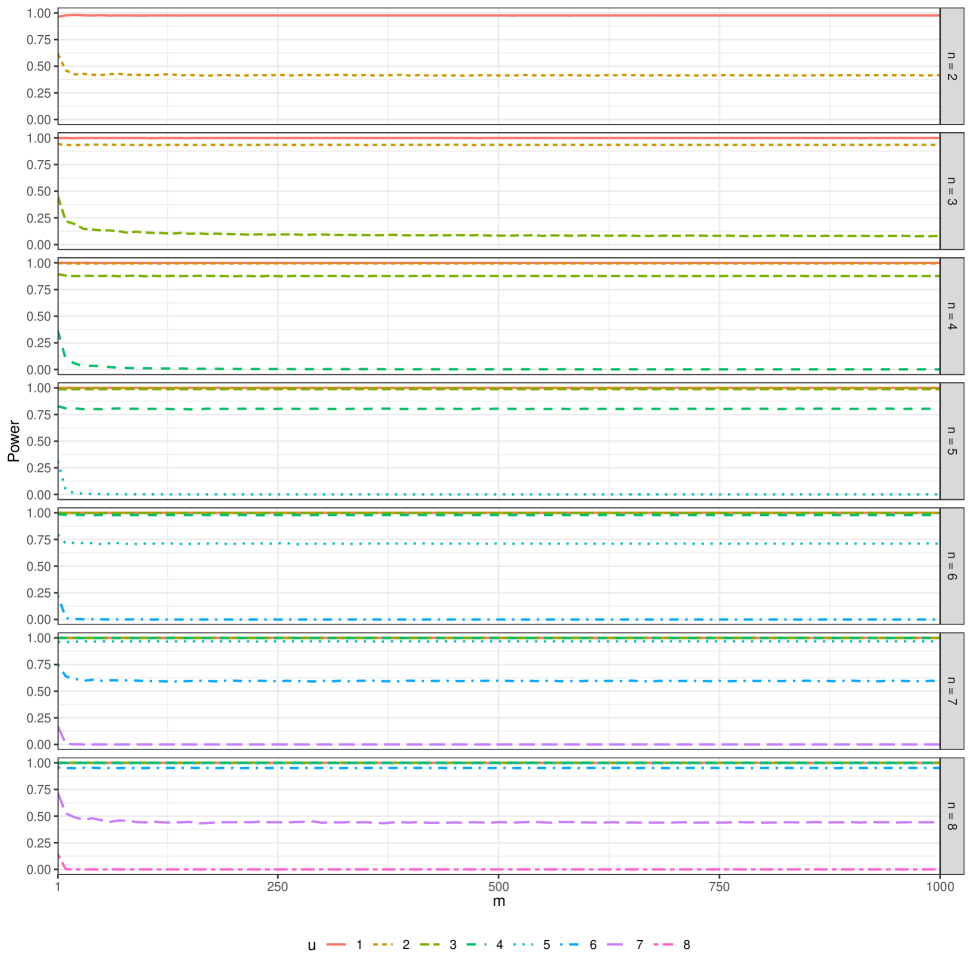
Figure E.1. Power of the BH procedure (with FDR target 0.05) applied to $m=1,10,20,\dots,1000$ Stouffer-GBHPC $p$-values under replicability levels $u=1,\dots,n$ for a simulation experiment with $n=2,3,\dots,8$ studies.

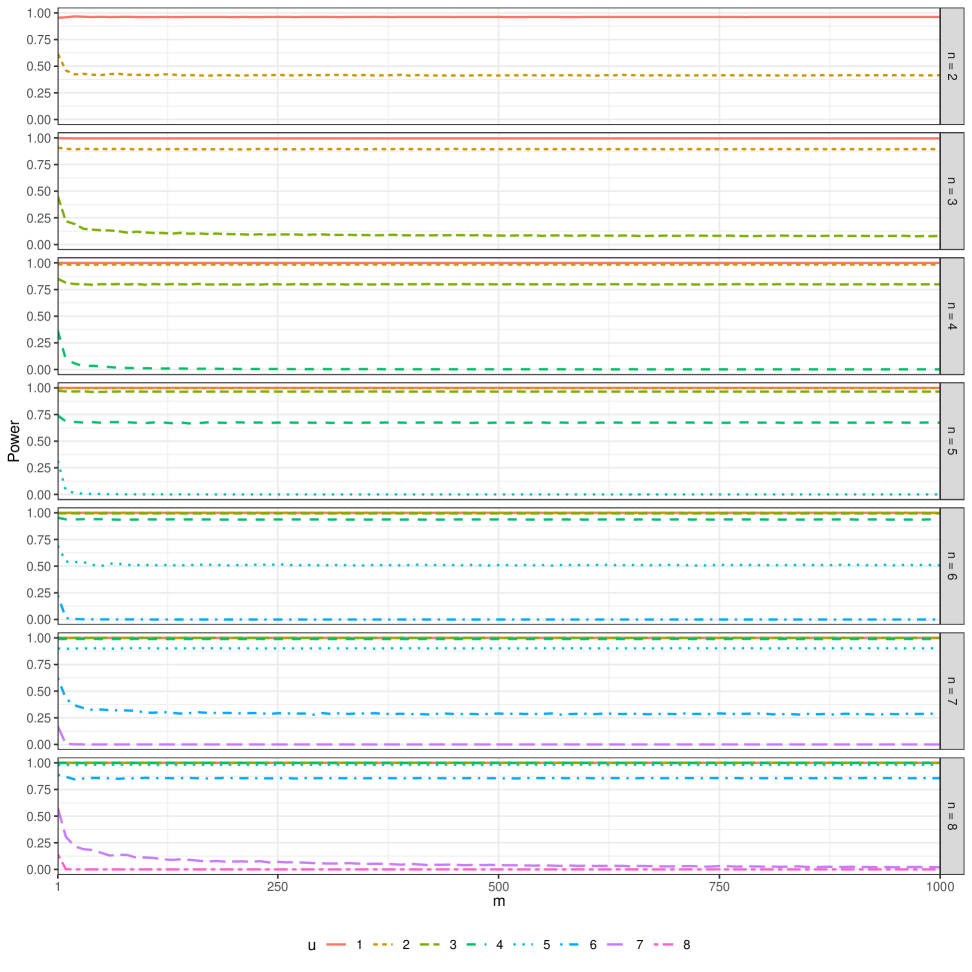
Figure E.2. Power of the BH procedure (with FDR target 0.05) applied to $m=1,10,20,\dots,1000$ Fisher-GBHPC $p$-values under replicability levels $u=1,\dots,n$ for a simulation experiment with $n=2,3,\dots,8$ studies.

Appendix F Additional simulations

F.1. Additional simulations for Section 4 for the case of $u<n$

We repeat the simulations described in Section 4 but with the following settings for $u$ and $n$:

$$(u,n)\in\{(2,3),(3,4),(3,5),(4,5)\}.$$

To accomodate for these new settings of $u$ and $n$, let the PC $p$-value for each feature $i\in[5000]$ be

$$p^{u/[n]}_{i}\equiv 1-\Phi\left(\frac{\sum_{j=u}^{n}\Phi^{-1}(1-p_{i(j)})}{\sqrt{n-u+1}}\right),$$

i.e., a GBHPC $p$-value (Definition 2) where each $f_{\mathcal{J}}$ is taken as Stouffer’s combining function. Moreover, let $\mathcal{U}(u)$ denote the set of all valid choices for $\mathbf{u}_{i}=(u_{i1},u_{i2})$ when $u$ is the replicability level and $K=2$ is the number of groups. For instance,

$$\mathcal{U}(4)=\{(1,3),(3,1),(2,2)\}.$$

We reimplement the ParFilter procedure described in item $(h)$ of Section 4.1, but under a new testing configuration where $K=2$, $\{\mathcal{G}_{k},w_{k}\}_{k\in[2]}$ is as specified in (A.2), and $\mathbf{u}_{i}$ sampled uniformly from $\mathcal{U}(u)$ for each $i\in[m]$. This version of the ParFilter enjoys finite-sample $\text{FDR}_{\text{rep}}$ control by Theorem A.1. All other methods from Section 4.1 are implemented as originally described, and their $\text{FDR}_{\text{rep}}$ guarantees, as summarized in Table 4.1, continue to hold.

The resulting empirical $\text{FDR}_{\text{rep}}$ and $\text{TPR}_{\text{rep}}$ results of this new set of simulations are presented in Figure F.1. When the covariates are non-informative ($\gamma_{1}=0$), we see that AdaFilter-BH (black line) outpowers the remaining methods, excluding the oracle (grey line), for all settings of $(u,n)$ and $\xi$. When the covariates are mildly ($\gamma_{1}=1.0$) or most ($\gamma_{1}=1.5$) informative, CAMT (purple line) and AdaPT (green line) display high levels of power, especially for $(u,n)\in\{(3,5),(4,5)\}$. The ParFilter (red line) generally exhibited weak power across all simulation settings, occasionally outperforming only BH (yellow line) and Inflated-AdaFilter-BH (dark blue line). Even when the covariates are the most informative ($\gamma_{1}=1.5$), its power remained significantly lower than that of AdaFilter-BH, a method that does not use covariates.

From these simulation results, it is evident that the ParFilter is not a competitive approach for $u<n$ replicability analyses, at least in our current implementation. We attribute this to the random selection of local replicability levels, rather than deriving them from covariates. This randomness leads to a large number of imbalanced features (Definition 5), which in turn diminishes the power of the ParFilter. Developing a general algorithm for constructing these levels using covariate information when $u<n$ would be a valuable direction for future research, though challenging due to the wide variability in the type, dimension, and informativeness of covariates across scientific contexts. In the meantime, CAMT and adaPT appear to be highly competitive choices for replicability analyses in the $u<n$ setting.

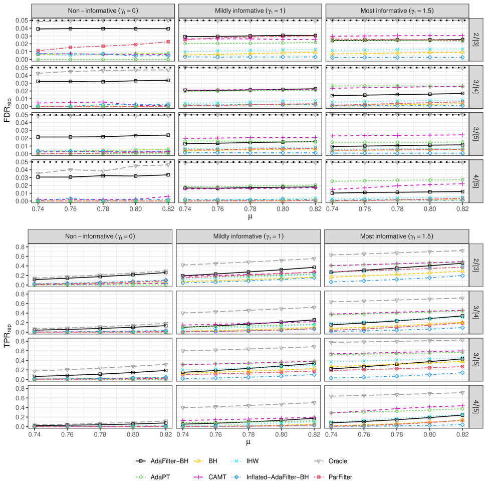
Figure F.1. $\text{FDR}_{\text{rep}}$ and $\text{TPR}_{\text{rep}}$ of the compared methods for the simulations in Appendix F.1 under $2/[3]$, $3/[4]$, $3/[5]$, and $4/5$ replicability; logistic parameters $\gamma_{1}=0,1,$ and $1.5$, denoted as non-informative, mildly informative, and most informative respectively; and effect size parameters $\xi=0.72,0.74,0.76,0.78,0.80,0.82$. Results are based on $500$ simulated datasets.

F.2. Simulation studies under negative AR(1) correlation

We repeat the simulations in Section 4 but inject $\mathbf{P}_{\cdot j}$ with autoregressive dependence of order 1, i.e., AR(1) correlation, for each study $j\in[n]$. The settings of $m$ and $(u,n)$, and the way we generate $\mathbf{X}$ and $\{I\{\text{$H_{ij}$ is true}\}\}_{(i,j)\in[m]\times[n]}$ remain exactly the same as in Section 4.

To generate the base $p$-values for each study $j$, we first generate $z$-scores $(z_{1j},\dots,z_{mj})$ with strong negative AR(1) correlation:

$$z_{ij}\sim\text{N}(0,1)\text{ for each $i\in[m]$}$$

where

$$\text{cor}(z_{ij},z_{i^{\prime}j})=(-0.8)^{|i-i^{\prime}|}\text{ for any $i,i^{\prime}\in[m]$.}$$

Across each study, the $z$-scores are independent, i.e., $(z_{1j},\dots,z_{mj})$ and $(z_{1j^{\prime}},\dots,z_{mj^{\prime}})$ are independent for any $j\neq j^{\prime}$. From the generated $z$-scores, we create base $p$-values by letting:

$$p_{ij}=\begin{cases}\Phi^{-1}(z_{ij})&\text{if $H_{ij}$ is true},\\ F^{-1}_{\text{Beta}}(z_{ij};1-\xi,7)&\text{if $H_{ij}$ is false,}\end{cases}\quad\text{for each $(i,j)\in[m]\times[n]$}$$

where $\Phi^{-1}(\cdot)$ is an inverse standard normal distribution and $F^{-1}_{\text{Beta}}(\cdot;\alpha_{1},\alpha_{2})$ is an inverse beta distribution with shape parameters $\alpha_{1}$ and $\alpha_{2}$. The range of the signal strength parameter is the same as in Section 4, i.e., $\xi\in\{0.72,0.74,0.76,0.78,0.80,0.82\}$. The base $p$-values defined above have the same marginal distribution as the base $p$-values defined in Section 4. But unlike Section 4, the base $p$-values generated here are negatively dependent within each study.

The methods explored in Section 4 are reimplemented in this simulation, excluding the oracle due to its computational complexity under dependence. In place of the oracle, we implemented a variant of the ParFilter procedure described in item $(h)$ of Section 4.1. This variant, which we refer to as the Inflated-ParFilter, differs from $(h)$ in the following ways: 1) the local PC weights are constructed according to Example 3.5 instead of Example 3.4, 2) the weighted null proportion estimators are taken in the form of (3.20) instead of (3.19), and 3) the tuning parameters are set to $\lambda_{k}=1$ for each $k\in[K]$ instead of $\lambda_{k}=0.5$. The Inflated-ParFilter has finite-sample $\text{FDR}_{\text{rep}}$ control under negative auto-regressive dependence as a consequence of Theorem 3.4. In contrast, the original ParFilter implementation described in $(h)$ does not.

We also replace the BH procedure with the Benjamini–Yekutieli (BY) procedure (Benjamini and Yekutieli,, 2001). The BY procedure modifies the BH threshold by inflating the target FDR level by a factor of $1/\left(\sum_{i=1}^{m}1/i\right)$. This inflation ensures that the BY procedure achieves finite-sample FDR control under arbitrary dependence among the $p$-values.

Among the five other methods compared (i.e., AdaFilter-BH, AdaPT, CAMT, IHW, and Inflated-AdaFilter-BH), Inflated-AdaFilter-BH, AdaFilter-BH, and CAMT have asymptotic control.

The results for this simulation are presented in Figure F.2. Overall, $\text{FDR}_{\text{rep}}$ control at $q=0.05$ was generally observed by every method. An exception is AdaFilter-BH (black line) under the setting $(n,\gamma_{1})=(2,0)$ (i.e., $2/[2]$ replicability with uninformative covariates) as its observed $\text{FDR}_{\text{rep}}$ exceeded $q=0.05$ for $\xi\in\{0.78,0.80,0.82\}$.

The power of the compared methods remains largely consistent with their performance in Section 4. Specifically, the ParFilter (red line) outperforms AdaFilter-BH when the covariates are mildly ($\gamma_{1}=1.0$) or most ($\gamma_{1}=1.5$) informative, while the AdaFilter-BH maintains its superior power when the covariates are non-informative ($\gamma_{1}=0$). The Inflated-ParFilter, the new method introduced in this section, exhibits poor power across all simulation settings, consistently outperforming only BY and Inflated-AdaFilter-BH. Recall that BY is the only other method guaranteed to control the finite-sample $\text{FDR}_{\text{rep}}$.

The simulation results indicate that our original implementation of the ParFilter (item $(h)$ of Section 4.1) has empirical $\text{FDR}_{\text{rep}}$ control under highly negatively correlated base $p$-values. A direction for future work is to investigate whether the ParFilter as implemented in item $(h)$ of Section 4.1 (or, more generally, under the algorithm settings described in Theorem 3.3$(i)$) has asymptotic $\text{FDR}_{\text{rep}}$ control under arbitrary dependence. If this is indeed the case, then implementing the Inflated-ParFilter may not be necessary for large-scale meta-analyses with many features, as it was shown here to have very low power.

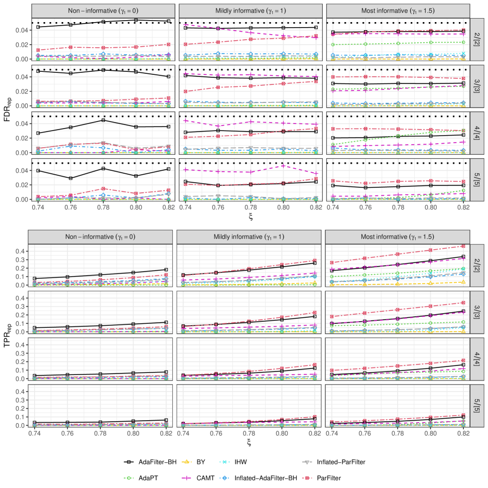
Figure F.2. $\text{FDR}_{\text{rep}}$ and $\text{TPR}_{\text{rep}}$ of the compared methods for the simulations in Appendix F.2 under $2/[2]$, $3/[3]$, $4/[4]$, $5/[5]$ replicability; logistic parameters $\gamma_{1}=0,1,$ and $1.5$, denoted as non-informative, mildly informative, and most informative respectively; and effect size parameters $\xi=0.72,0.74,0.76,0.78,0.80,0.82$. Results are based on $500$ simulated datasets.

References

• Akiyama et al., (2013) Akiyama, T., Shinzawa, M., Qin, J., and Akiyama, N. (2013). Regulations of gene expression in medullary thymic epithelial cells required for preventing the onset of autoimmune diseases. Front Immunol, 4:249.
• Anderson et al., (2002) Anderson, M. S., Venanzi, E. S., Klein, L., Chen, Z., Berzins, S. P., Turley, S. J., von Boehmer, H., Bronson, R., Dierich, A., Benoist, C., and Mathis, D. (2002). Projection of an immunological self shadow within the thymus by the aire protein. Science, 298(5597):1395–1401.
• Benjamini and Heller, (2008) Benjamini, Y. and Heller, R. (2008). Screening for partial conjunction hypotheses. Biometrics, 64(4):1215–1222.
• Benjamini et al., (2009) Benjamini, Y., Heller, R., and Yekutieli, D. (2009). Selective inference in complex research. Philosophical transactions. Series A, Mathematical, physical, and engineering sciences, 367:4255–71.
• Benjamini and Hochberg, (1995) Benjamini, Y. and Hochberg, Y. (1995). Controlling the false discovery rate: A practical and powerful approach to multiple testing. Journal of the Royal Statistical Society. Series B (Methodological), 57(1):289–300.
• Benjamini and Hochberg, (1997) Benjamini, Y. and Hochberg, Y. (1997). Multiple hypotheses testing with weights. Scandinavian Journal of Statistics, 24(3):407–418.
• Benjamini and Yekutieli, (2001) Benjamini, Y. and Yekutieli, D. (2001). The control of the false discovery rate in multiple testing under dependency. The Annals of Statistics, 29(4):1165–1188.
• Blanchard and Roquain, (2008) Blanchard, G. and Roquain, E. (2008). Two simple sufficient conditions for fdr control. Electronic Journal of Statistics, 2.
• Blanchard and Roquain, (2009) Blanchard, G. and Roquain, E. (2009). Adaptive false discovery rate control under independence and dependence. Journal of Machine Learning Research, 10(97):2837–2871.
• Bogomolov, (2023) Bogomolov, M. (2023). Testing partial conjunction hypotheses under dependency, with applications to meta-analysis. Electronic Journal of Statistics, 17(1):102 – 155.
• Bogomolov and Heller, (2018) Bogomolov, M. and Heller, R. (2018). Assessing replicability of findings across two studies of multiple features. Biometrika, 105(3):505–516.
• Bogomolov and Heller, (2023) Bogomolov, M. and Heller, R. (2023). Replicability Across Multiple Studies. Statistical Science, 38(4):602 – 620.
• Derbinski et al., (2005) Derbinski, J., Gäbler, J., Brors, B., Tierling, S., Jonnakuty, S., Hergenhahn, M., Peltonen, L., Walter, J., and Kyewski, B. (2005). Promiscuous gene expression in thymic epithelial cells is regulated at multiple levels. J Exp Med, 202(1):33–45.
• Efron, (2008) Efron, B. (2008). Microarrays, Empirical Bayes and the Two-Groups Model. Statistical Science, 23(1):1 – 22.
• Feng et al., (2024) Feng, B., Zhang, Y., Qiao, L., Tang, Q., Zhang, Z., Zhang, S., Qiu, J., Zhou, X., Huang, C., and Liang, Y. (2024). Evaluating the significance of ecscr in the diagnosis of ulcerative colitis and drug efficacy assessment. Frontiers in Immunology, 15.
• Fisher, (1973) Fisher, R. A. (1973). Statistical methods for research workers. Hafner Publishing Co., New York, fourteenth edition.
• Friston et al., (2005) Friston, K. J., Penny, W. D., and Glaser, D. E. (2005). Conjunction revisited. NeuroImage, 25(3):661–667.
• Genovese et al., (2006) Genovese, C. R., Roeder, K., and Wasserman, L. (2006). False discovery control with p-value weighting. Biometrika, 93(3):509–524.
• Gruper et al., (2023) Gruper, Y., Wolff, A. S. B., Glanz, L., Spoutil, F., Marthinussen, M. C., Osickova, A., Herzig, Y., Goldfarb, Y., Aranaz-Novaliches, G., Dobeš, J., Kadouri, N., Ben-Nun, O., Binyamin, A., Lavi, B., Givony, T., Khalaila, R., Gome, T., Wald, T., Mrazkova, B., Sochen, C., Besnard, M., Ben-Dor, S., Feldmesser, E., Orlova, E. M., Hegedűs, C., Lampé, I., Papp, T., Felszeghy, S., Sedlacek, R., Davidovich, E., Tal, N., Shouval, D. S., Shamir, R., Guillonneau, C., Szondy, Z., Lundin, K. E. A., Osicka, R., Prochazka, J., Husebye, E. S., and Abramson, J. (2023). Autoimmune amelogenesis imperfecta in patients with aps-1 and coeliac disease. Nature, 624(7992):653–662.
• Heinlein et al., (2022) Heinlein, M., Gandolfo, L. C., Zhao, K., Teh, C. E., Nguyen, N., Baell, J. B., Goldfarb, Y., Abramson, J., Wichmann, J., Voss, A. K., Strasser, A., Smyth, G. K., Thomas, T., and Gray, D. H. D. (2022). The acetyltransferase KAT7 is required for thymic epithelial cell expansion, expression of AIRE target genes, and thymic tolerance. Sci Immunol, 7(67):eabb6032.
• Heller and Rosset, (2020) Heller, R. and Rosset, S. (2020). Optimal Control of False Discovery Criteria in the Two-Group Model. Journal of the Royal Statistical Society Series B: Statistical Methodology, 83(1):133–155.
• Ignatiadis and Huber, (2021) Ignatiadis, N. and Huber, W. (2021). Covariate Powered Cross-Weighted Multiple Testing. Journal of the Royal Statistical Society Series B: Statistical Methodology, 83(4):720–751.
• Jéru et al., (2014) Jéru, I., Cochet, E., Duquesnoy, P., Hentgen, V., Copin, B., Mitjavila-Garcia, M. T., Sheykholeslami, S., Le Borgne, G., Dastot-Le Moal, F., Malan, V., Karabina, S., Mahevas, M., Chantot-Bastaraud, S., Lecron, J.-C., Faivre, L., and Amselem, S. (2014). Brief report: Involvement of TNFRSF11A molecular defects in autoinflammatory disorders. Arthritis Rheumatol, 66(9):2621–2627.
• Katsevich et al., (2023) Katsevich, E., Sabatti, C., and Bogomolov, M. (2023). Filtering the rejection set while preserving false discovery rate control. Journal of the American Statistical Association, 118(541):165–176.
• Klein et al., (2014) Klein, L., Kyewski, B., Allen, P. M., and Hogquist, K. A. (2014). Positive and negative selection of the t cell repertoire: what thymocytes see (and don’t see). Nature Reviews Immunology, 14(6):377–391.
• Lei and Fithian, (2018) Lei, L. and Fithian, W. (2018). AdaPT: An Interactive Procedure for Multiple Testing with Side Information. Journal of the Royal Statistical Society Series B: Statistical Methodology, 80(4):649–679.
• Miyazawa et al., (2023) Miyazawa, R., Nagao, J.-i., Arita-Morioka, K.-i., Matsumoto, M., Morimoto, J., Yoshida, M., Oya, T., Tsuneyama, K., Yoshida, H., Tanaka, Y., and Matsumoto, M. (2023). Dispensable Role of Aire in CD11c+ Conventional Dendritic Cells for Antigen Presentation and Shaping the Transcriptome. ImmunoHorizons, 7(1):140–158.
• Muro et al., (2024) Muro, R., Nitta, T., Nitta, S., Tsukasaki, M., Asano, T., Nakano, K., Okamura, T., Nakashima, T., Okamoto, K., and Takayanagi, H. (2024). Transcript splicing optimizes the thymic self-antigen repertoire to suppress autoimmunity. The Journal of Clinical Investigation, 134(20).
• Orabona and Jun, (2024) Orabona, F. and Jun, K.-S. (2024). Tight concentrations and confidence sequences from the regret of universal portfolio. IEEE Transactions on Information Theory, 70(1):436–455.
• Pashler and Harris, (2012) Pashler, H. and Harris, C. R. (2012). Is the replicability crisis overblown? three arguments examined. Perspectives on Psychological Science, 7(6):531–536. PMID: 26168109.
• Ramdas et al., (2019) Ramdas, A. K., Barber, R. F., Wainwright, M. J., and Jordan, M. I. (2019). A unified treatment of multiple testing with prior knowledge using the p-filter. The Annals of Statistics, 47(5):2790 – 2821.
• Ritchie et al., (2015) Ritchie, M. E., Phipson, B., Wu, D., Hu, Y., Law, C. W., Shi, W., and Smyth, G. K. (2015). limma powers differential expression analyses for RNA-sequencing and microarray studies. Nucleic Acids Research, 43(7):e47–e47.
• Roquain and van de Wiel, (2008) Roquain, É. and van de Wiel, M. A. (2008). Optimal weighting for false discovery rate control. Electronic Journal of Statistics, 3:678–711.
• Simes, (1986) Simes, R. J. (1986). An improved Bonferroni procedure for multiple tests of significance. Biometrika, 73(3):751–754.
• Smyth, (2004) Smyth, G. K. (2004). Linear models and empirical bayes methods for assessing differential expression in microarray experiments. Stat Appl Genet Mol Biol, 3:Article3.
• Stouffer et al., (1949) Stouffer, S., Suchman, E., DeVinney, L., and S.A. Star, R. W. J. (1949). The american soldier: Adjustment during army life". Studies in Social Pyschologu in World War II, 1.
• Sun and Cai, (2007) Sun, W. and Cai, T. T. (2007). Oracle and adaptive compound decision rules for false discovery rate control. Journal of the American Statistical Association, 102(479):901–912.
• Tischner et al., (2010) Tischner, D., Woess, C., Ottina, E., and Villunger, A. (2010). Bcl-2-regulated cell death signalling in the prevention of autoimmunity. Cell Death & Disease, 1(6):e48–e48.
• Wang et al., (2022) Wang, J., Gui, L., Su, W. J., Sabatti, C., and Owen, A. B. (2022). Detecting multiple replicating signals using adaptive filtering procedures. The Annals of Statistics, 50(4):1890 – 1909.
• Wang and Owen, (2019) Wang, J. and Owen, A. B. (2019). Admissibility in partial conjunction testing. Journal of the American Statistical Association, 114(525):158–168.
• Wang and Ramdas, (2022) Wang, R. and Ramdas, A. (2022). False Discovery Rate Control with E-values. Journal of the Royal Statistical Society Series B: Statistical Methodology, 84(3):822–852.
• Waudby-Smith and Ramdas, (2023) Waudby-Smith, I. and Ramdas, A. (2023). Estimating means of bounded random variables by betting. Journal of the Royal Statistical Society Series B: Statistical Methodology, 86(1):1–27.
• Weiss, (1965) Weiss, L. (1965). On the asymptotic distribution of the largest sample spacing. Journal of the Society for Industrial and Applied Mathematics, 13(3):720–731.
• Weiss, (1969) Weiss, L. (1969). The joint asymptotic distribution of the k-smallest sample spacings. Journal of Applied Probability, 6(2):442–448.
• Zhang and Chen, (2022) Zhang, X. and Chen, J. (2022). Covariate adaptive false discovery rate control with applications to omics-wide multiple testing. Journal of the American Statistical Association, 117(537):411–427.