Thermal emission effect on Chandrasekhar’s -function for isotropic scattering in semi-infinite atmosphere problem
Abstract
Chandrasekhar’s -function has long been a cornerstone of radiative transfer theory in semi-infinite, isotropically scattering atmospheres subjected to external illumination. However, this classical formulation does not account for thermal emission arising from internal heat sources, which is critical in a variety of astrophysical contexts—such as hot Jupiters, brown dwarfs, and irradiated exoplanets—where the re-radiation of absorbed stellar energy significantly alters the emergent intensity. To address this limitation, we extend the diffuse reflection framework to incorporate both isotropic scattering and intrinsic thermal emission, leading to a generalized function known as the -function. Building on the formalism of Chandrasekhar (1960) combined with the recent work by Sengupta (2021), we derive the governing integral equations for the -function and express it in terms of three key physical parameters: the radiation direction cosine , the thermal emission coefficient , and the single scattering albedo . We implement a numerically stable iterative scheme, using Gaussian quadrature method to compute high-precision values of across a broad parameter space. In the zero-emission limit, our results recover the classical -function, thus validating the method. We provide comprehensive values of -function for , , and , enabling direct application to modeling diffusely reflected intensities from thermally emitting atmospheres. As a case study, we apply this formalism to exoplanet K2-137b and identify the wavelength range (0.85–2.5 m) where the model is most applicable, highlighting its relevance to the observation range of the telescopes JWST, HST, ARIEL.
1 Introduction
Radiative transfer theory stands as a cornerstone of modern astrophysics, providing the mathematical and physical framework necessary to understand radiation propagation through scattering and absorbing media as shown in the classical works by Chandrasekhar (1960) and Mihalas (1978). Its relevance extends across the astrophysical spectrum—from stellar interiors and photospheres to planetary and exoplanetary atmospheres. In particular, the foundational work presented in Chandrasekhar (1960) on radiative transfer in a semi-infinite atmosphere, and the introduction of the Chandrasekhar -function, has had enduring significance. The -function, where is the direction cosine of the angle between the scattering plane and the pencil of radiation originally formulated to describe diffuse reflection in scattering media, remains central to contemporary models of planetary reflection and energy balance.
In the astrophysical context, the theory of radiative transfer is indispensable—from the study of the Sun to the study of exoplanets. Classical solutions, while powerful, must be revisited in environments where internal heating or thermal emission cannot be ignored. Bellman et al. (1967) extended the original Chandrasekhar planetary problem to include internal heating sources, paving the way for incorporating thermal emission into the diffuse reflection framework.
This extension is particularly relevant in the context of irradiated giant exoplanets such as Hot Jupiters, where anomalously inflated radii point toward significant internal heat sources (Komacek & Youdin, 2017; Batygin & Stevenson, 2010). For habitable worlds and Hot Jupiters alike, transmission and reflection spectroscopy are key observational tools, and the diffuse reflection theory of Chandrasekhar (1960) continues to serve as the theoretical backbone in these analyses (Singla et al., 2023; Singla & Sengupta, 2023). Even the theory is directly useful in modeling the planetary atmosphere Madhusudhan & Burrows (2012) as well as to determine the amount of heat redistribution through convection in the tidally locked hot Jupiters Sengupta & Sengupta (2023).
Chandrasekhar’s -function has also found broader applications beyond planetary atmospheres. For instance, Jablonski (2019) demonstrated its utility in modeling photoelectron transport, while Jablonski (2015) presented a numerically stable and precise method for its evaluation in the isotropic scattering limit. The theoretical structure surrounding the -function, including its integral properties, iterative solutions (Bosma & De Rooij, 1983), and moment expansions (Anlı & Öztürk, 2021), has been rigorously studied. Its values for both isotropic and asymmetric scattering scenarios are tabulated in Chandrasekhar & Breen (1947, 1948), with detailed discussion of the function’s moments and derivatives with better accuracy is in Das & Bera (2007).
Furthermore, Chandrasekhar’s semi-infinite atmosphere theory finds direct application in areas ranging from planetary atmosphere modeling to secondary electron emission in ion-solid interactions (Dubus et al., 1986). Nevertheless, traditional formulations of the -function fail to capture scenarios where thermal emission and scattering are comparably significant.
This shortfall was first addressed in Sengupta (2021), where it was shown that thermal emission alters the source function in the semi-infinite diffuse reflection problem by contributing an additive term , where is a function of the direction cosine . For the case of isotropic scattering, they established a specific functional form , introducing what is now referred to as the -function, analogous in form to the classical -function but extended to account for thermal emission. The diffusely reflected specific intensity from a thermally emitting, isotropically scattering, semi-infinite atmosphere is given by Sengupta (2021):
| (1) |
Here, is the incident flux along the direction , while the diffuse reflection is observed along . The dimensionless thermal emission coefficient is defined as , where is the Planck function. The -function introduced in this context is a function of , , and the single scattering albedo , i.e. distinguishing it from the classical -function as given in Chandrasekhar (1960).
The physical interpretation and formal structure of were further discussed in Sengupta (2022) in relation to generalized and functions used for finite atmosphere models. However, those studies remained primarily qualitative. To date, no comprehensive effort has been made to quantify the -function in its full parametric dependence for practical use in astrophysical applications.
In this work, we resolve this gap by formulating a rigorous derivation and complete numerical evaluation of the function as defined in Sengupta (2021). We adopt a methodology parallel to that employed by Chandrasekhar (1960) in the classical treatment of the -function: first deriving the integral theorems governing the -function, then treating it as a function of three physical parameters—, , and . We compute its values across a physically meaningful range of these parameters. These tabulated values are directly applicable in calculating reflected specific intensities via Eq. (1), thus equipping the community with a practical tool for modeling thermal emission and scattering in planetary and exoplanetary atmospheres. The results presented here are fully consistent with, and extend beyond, the well-established literature on classical radiative transfer.
The plan of the paper goes as follows. In Section 2, we have derived the theorems applicable for function introduced in Sengupta (2021).Section 3 is devoted in estimating the values of M as a function of direction cosine , thermal emission co-efficient U and single scattering albedo . For simplicity, this section is further divided into three subsections and discussed only emission in 3.1, only scattering in 3.2 and simultaneous emission as well as scattering in 3.3. In section 4, we discussed the consistency limit of our results with the previous studies. Finally we concluded by discussing the results, limitation and future works in Section 5 follows with a general conclusion in Section 6
2 Theorems of M-Function
Here we will write the function as for simplifying the mathematical expressions. However the meaning remains the same. The functional form of -function is defined as Sengupta (2021),
| (2) |
Here we define the moments of M-function as follows,
| (3) |
and the thermal emission contribution to the values of M-function,
| (4) |
Theorem 1.
The integration of M-function can be written as,
| (5) |
Proof.
Multiplying eqn.(2) by in both side and taking integration over in the limit 0 to 1 we will get,
Now interchanging the and and taking the average we will get,
This is a quadratic equation which has a solution as follows,
| (6) |
In eqn.(6) the left hand side uniformly converges to zero, when the single scattering albedo uniformly goes to zero. To satisfy the fact from the right side expression as well we will consider the negative sign rather than the positive sign. Thus it can be written as,
| (7) |
In this equation if we use eqn.(4) for the expression R we will get the simplified form as,
Corollary 1.1.
The necessary condition for which the -function will be real can be written as,
| (8) |
Proof.
Corollary 1.2.
An alternative integral equation can be formed as,
| (9) |
Proof.
The final form is equivalent to the eqn.(9) ∎
Corollary 1.3.
The zeroth order moment of the M-function can be represented as,
| (10) |
This represents the expression of the zeroth order moment .
Theorem 2.
| (12) |
3 Estimation of the values of M-function:
In this section we will derive the values of in a range of parameter values , and U. From now on we will write the thermal emission co-efficient just as U for simplicity with the knowledge of how this function is defined. Hence the explicit expression of M-function can be written as,
| (14) |
To progress further we will make it simple by classifying in three different regions as follows,
- •
- •
- •
Note that eqn. (14) consists of natural logarithm with base e as per the calculations presented in Sengupta (2021). Hence all the following calculations are done in , simply written as log to remain consistent with the literature, unless otherwise noted.
3.1 Only emission:
This is the simplest one among the three and can be solved analytically. For only emission case we can consider the scattering albedo,
Hence the equation of function will be,
| (15) |
At this point we note that, eqn.(15) has to give a positive value of otherwise the emitting radiation will be negative which is unphysical. This puts the following condition on the denominator,
| (16) |
For the range of [0:1], we will get the maximum value of at . Hence the above condition will reduce into,
| (17) |
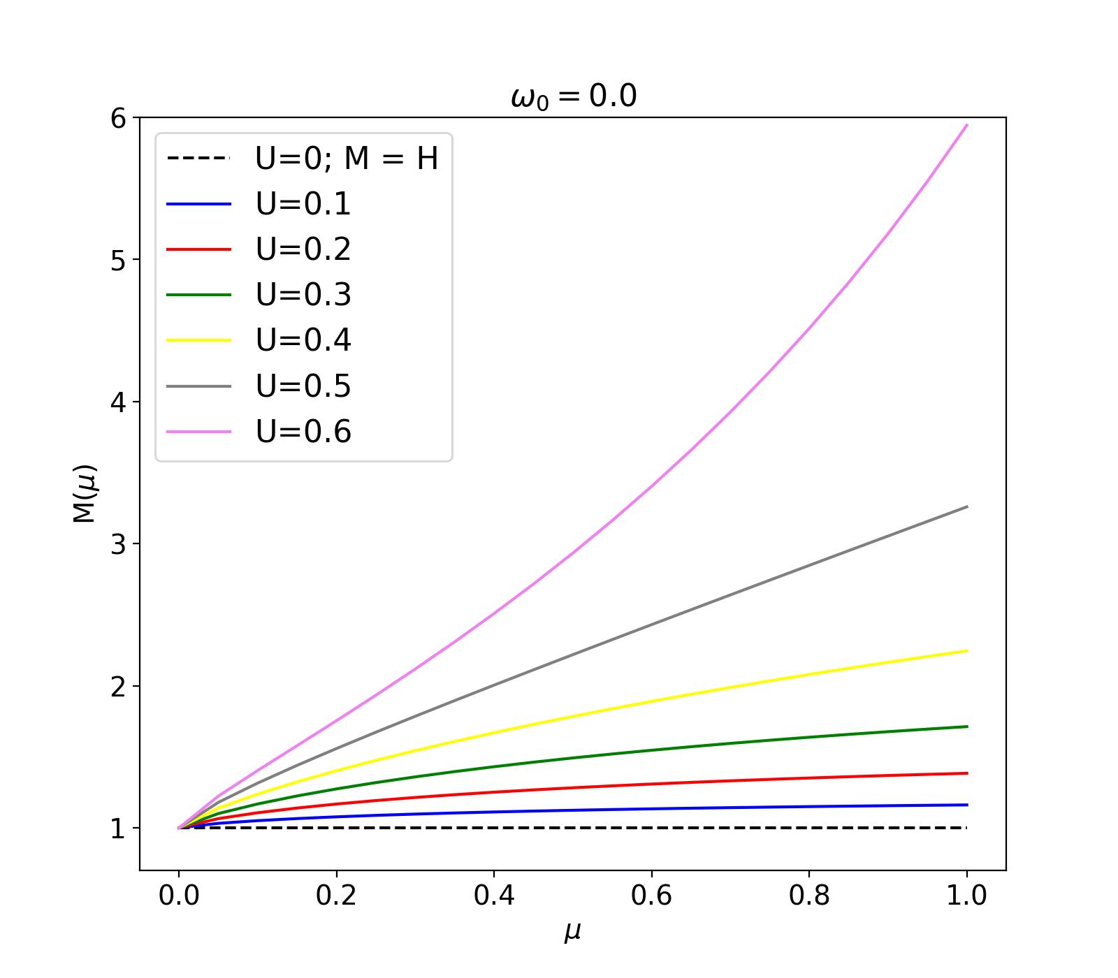
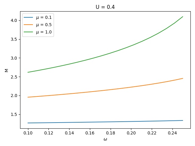
It means that for only emission case there is an upper limit of the blackbody flux to the irradiated flux ratio to get the real values of -function which can be written as , . In figure 1(a) we have shown M as a function of for only emission case with varying U values upto 0.6 respecting the boundary set by the inequality condition eqn. (17). We will see a similar but more general condition for simultaneous emission and scattering as discussed in 3.3
3.2 Only scattering:
In only scattering case we can consider the thermal emission contribution U=0 and thus the will reduce into,
| (18) |
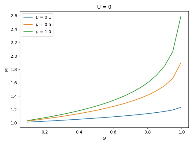
This is nothing but Chandrasekhar’s -function in isotropic scattering case as shown in eqn.(22). In fact in the no emission limit , as discussed in section 4 . Clearly eqn.(22) is a non-linear equation and its values can not be derived analytically. However the values of this function is well derived and tabulated in Chandrasekhar & Breen (1947).In this article these values are revisited in case of no emission, for single scattering albedo values to 0.95. Only for perfect scattering case case we need 3163 iterations for convergence (Not shown here), see 5. In figure.3, the plot representing U=0 shows the variation of with respect to for fixed s. Its variation with for fixed are also plotted by dashed lines in each plots of figure 1
3.3 Simultaneous emission and scattering
This is the most general case to be discussed in this article. The derived values exactly match with the previously derived values at the limiting conditions of only emission and only scattering. Here we solved the general equation of M-function as given in eqn. (14). Clearly this is a three variable non-linear equation which can only be solved numerically. The integral equation has been solved using the Gauss-Legendre quadrature method for 100 points, with convergence tolerance . All the numerical simulations has been done using the open source python packages numpy and Scipy. For numerical simulations we limit ourselves with maximum iterations 1000 which gives us quite satisfactory results. However the values are same as function as represented by Chandrasekhar (1960).
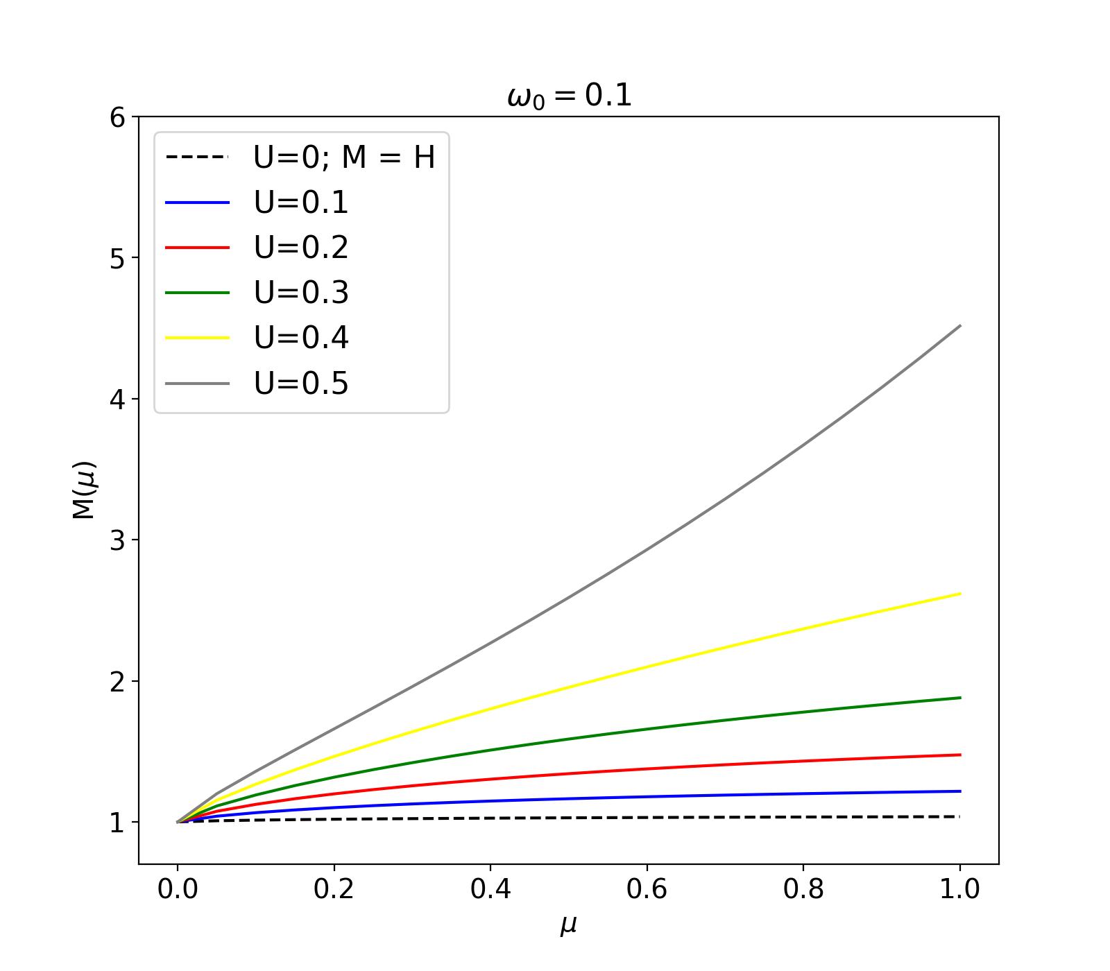
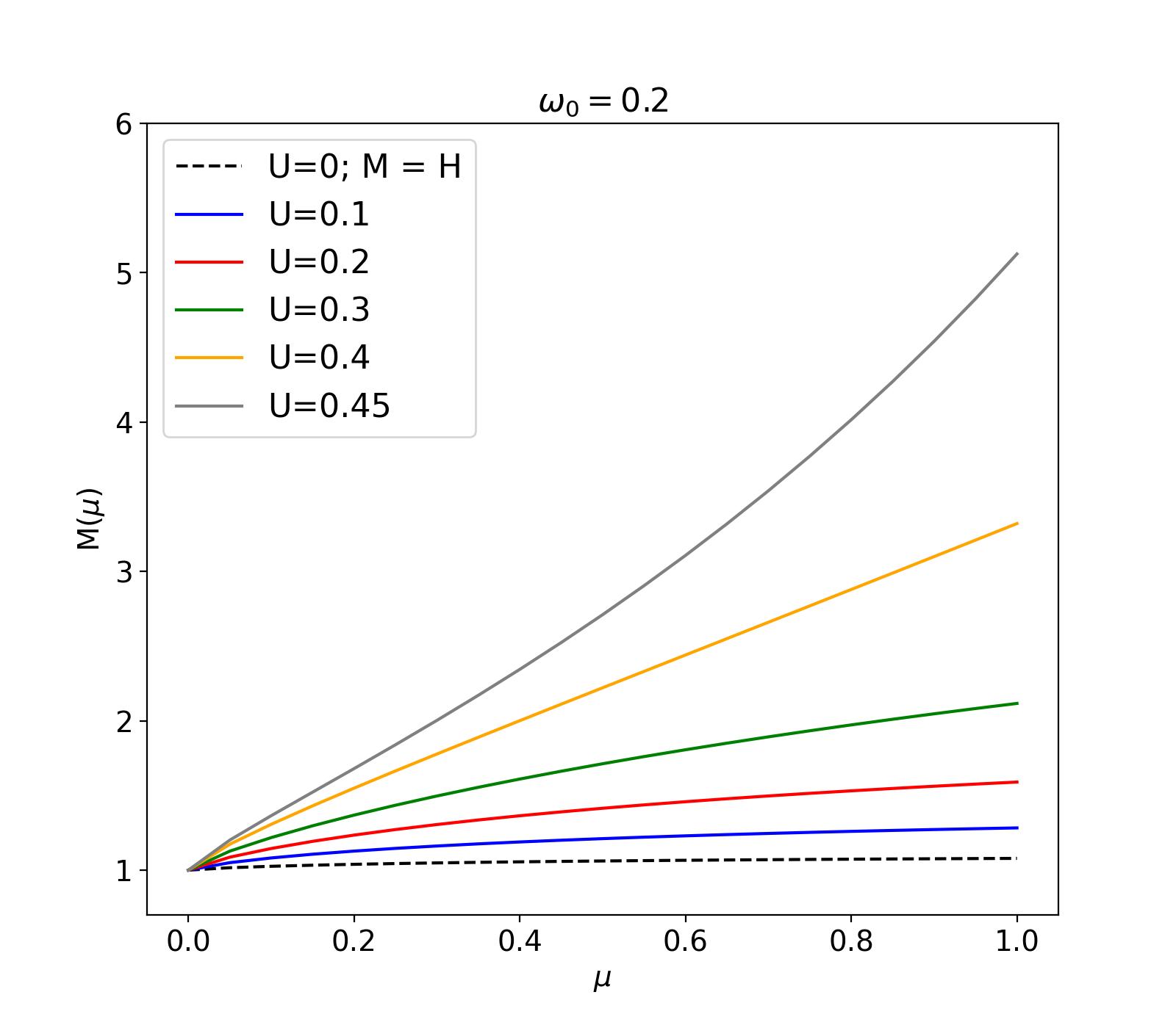
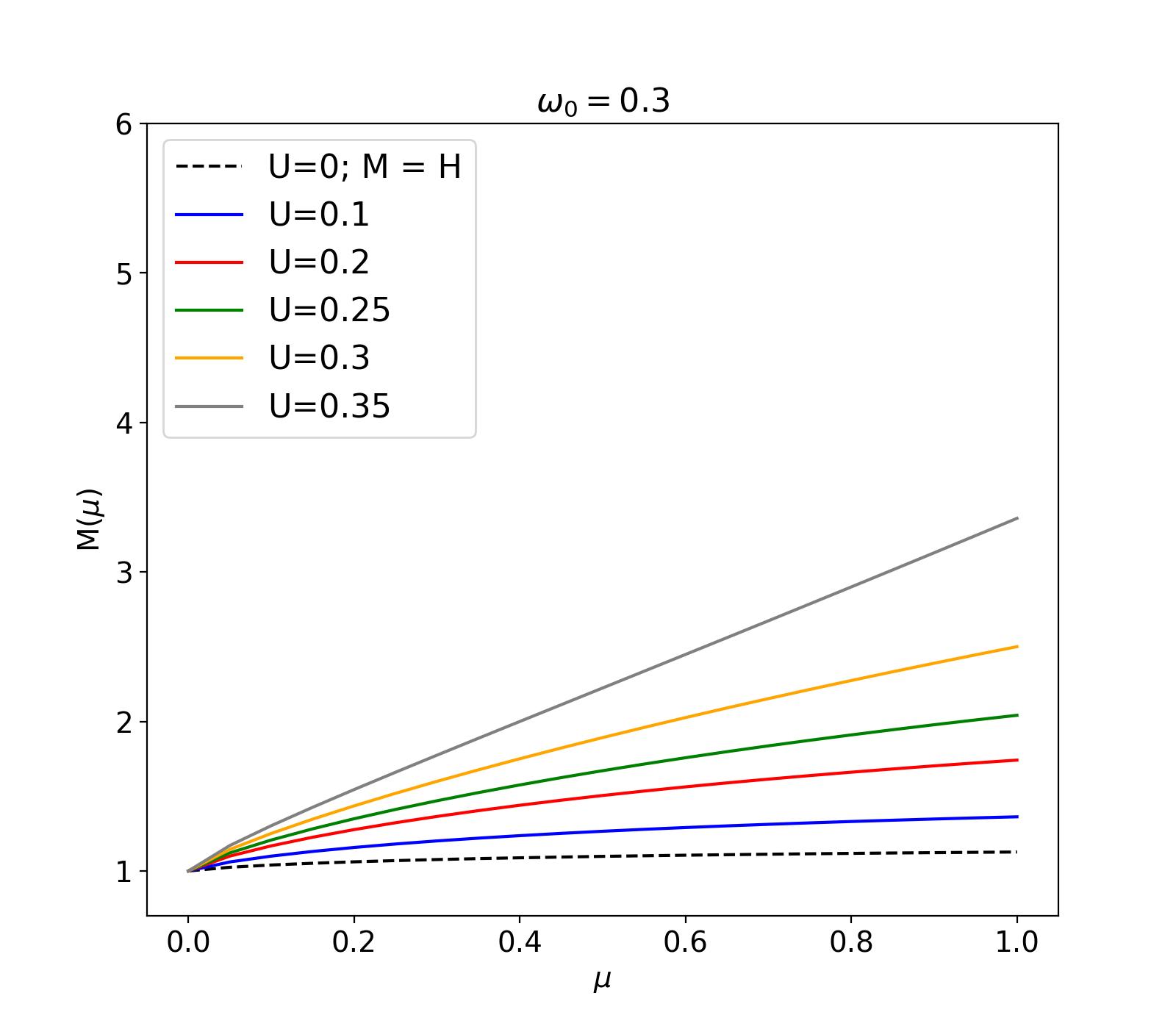
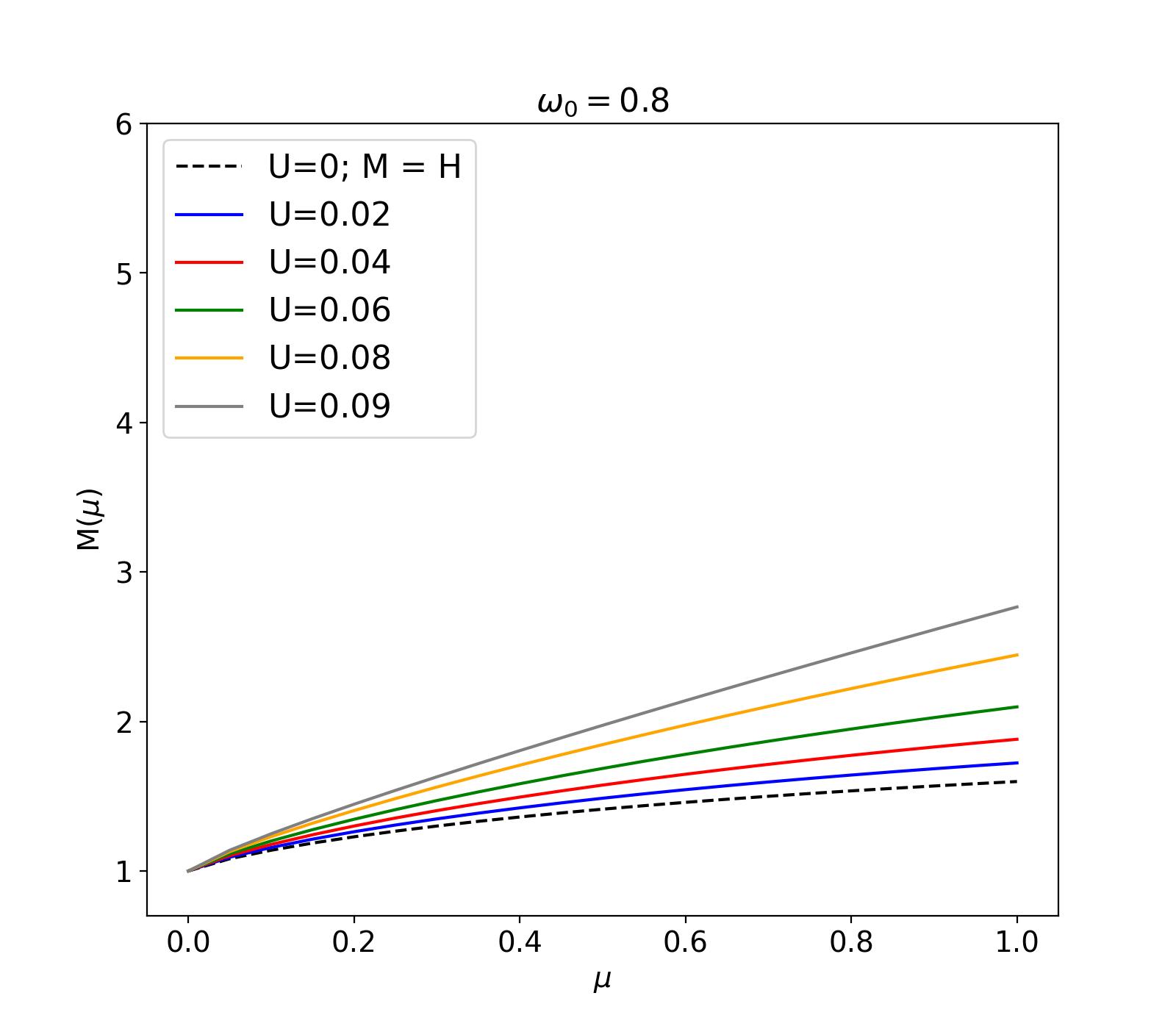
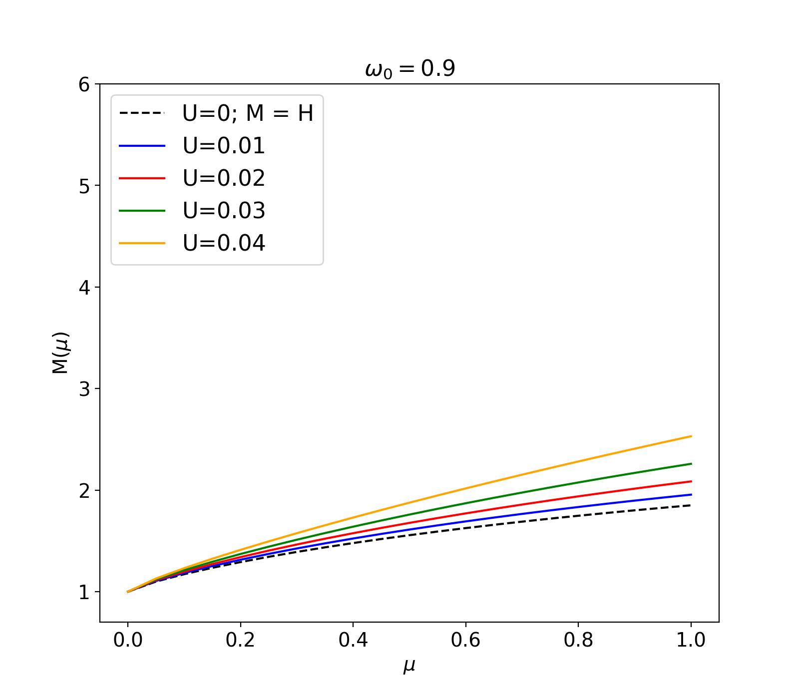
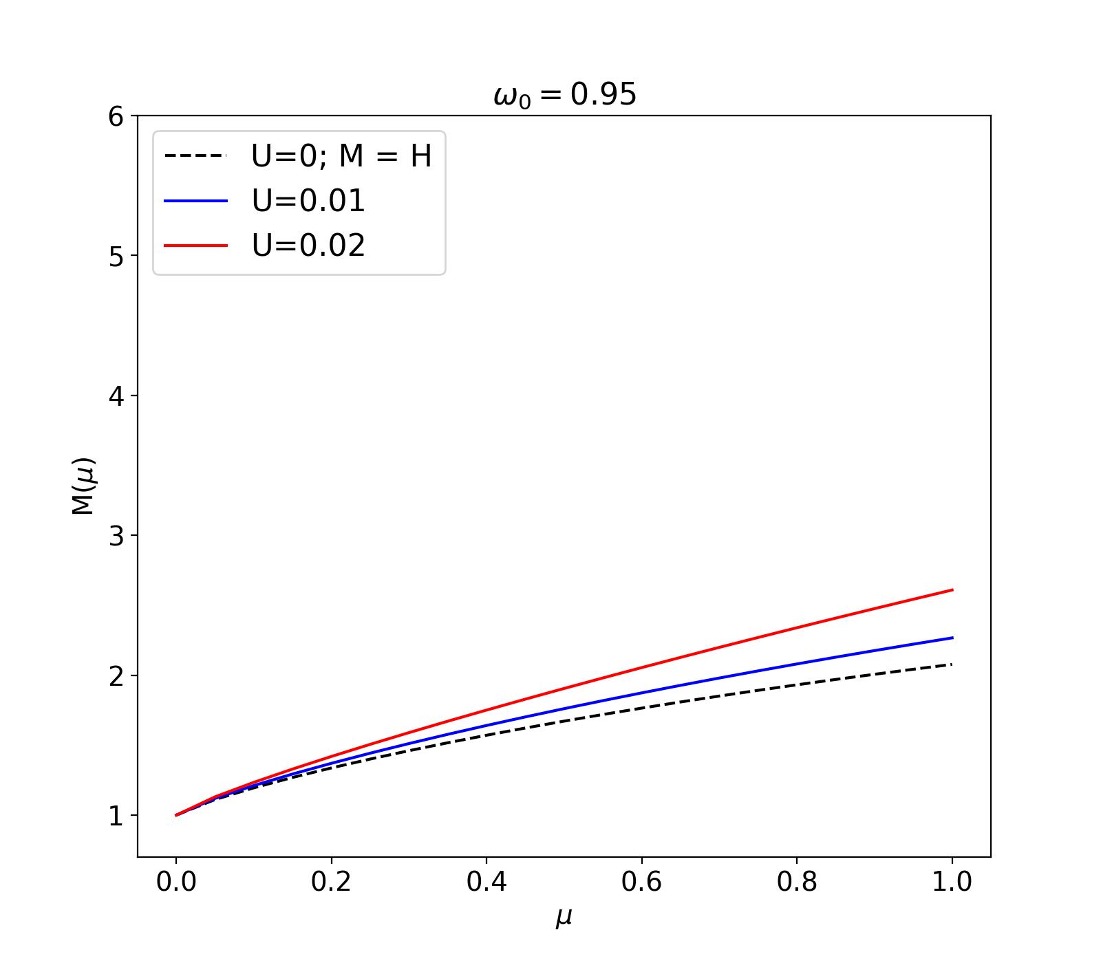
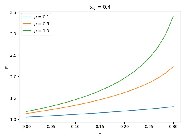
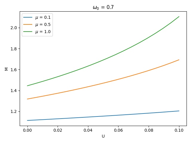
While varying the we remind that the values of M will be real only within the regime constrained by Corollary1.1. Taking account of that we calculated the M-values for = 0.1, 0.2,0.3,0.4,0.5,0.6,0.7,0.8,0.9,0.95 respectively along with the maximum possible U (named ) for the convergence in the corresponding tables. It can be seen from fig.1 that, for real , decreases with increasing satisfying the condition of corollary 1.1. The tabulated values of are plotted in figure 1
4 Consistency of our results
We have derived the theorems and values of the function which are more general than Chandrasekhar’s -function in case of isotropic scattering, where we have added thermal emission along with the scattering. Now we show that at the low thermal emission limit i.e. all of our results will match with that of the function.
In case of diffusion scattering, the well known Chandrasekhar’s H-function can be written Chandrasekhar (1960) as,
| (19) |
where represents the characteristic function and satisfying the condition
| (20) |
and
| (21) |
In case of isotropic scattering, , where is the single scattering albedo. Now the functional form of H-function will be, (see Chandrasekhar (1960)pg. 97)
| (22) |
| (23) |
and
| (24) |
Also the moments of H-function are defined in Chandrasekhar (1960) as
satisfy the relation in case of isotropic scattering (viz. pg. 109 of Chandrasekhar (1960)). Evaluating and considering the negative sign to take the fact that uniformly goes to zero with we get,
| (25) |
In section 2, we derived the integral theorems of M-function which are analogous to Chandrasekhar’s H-function in case of simultaneous thermal emission and diffusely scattering atmosphere. To be consistent with Chandrasekhar’s results as shown here, the theorems for M-function should match with the integral theorems of H-functions in isotropic scattering case for no thermal emission limit.
At the limit of low thermal emission, i.e. , and hence according to eqn.(4). In such case the integral theorems of M-functions will reduce into,
and
These matches exactly with the theorems of H-function for isotropic case eqns. (23),(24). Also at low thermal emission the moment of function eqn.(10) shows that putting the limit
Finally we discuss the consistency of the values of the -function as shown in fig. 1. The methods of derivation of the values has been discussed in section 3. In each plot the line representing U = 0.0 provides the values of which are exactly the same as the values of provided by Chandrasekhar & Breen (1947) for the isotropic scattering case with corresponding values of . Also the left panel of figure. 3 exactly reproduces the function in the no thermal emission limit. Hence all of our results are fully consistent with the function for the no thermal emission (i.e. ) limit.
5 Discussion
In this work, we have derived and established a set of theorems governing the behavior of the function, which incorporates both isotropic scattering and thermal emission in the context of semi-infinite diffuse reflection problem. This marks a significant step forward by integrating the thermal emission contribution, represented by the coefficient , where is the thermal emission and is the irradiated flux, into the classical scattering framework introduced by Chandrasekhar (1960). The inclusion of this term modifies the traditional radiative transfer equations and introduces a new layer of complexity, which is particularly relevant in astrophysical scenarios such as exoplanets and Hot Jupiters, where internal heating significantly impacts the emergent radiation.
5.1 Theorems and their Physical Significance
The derived theorems governing the function are consistent with the established works on radiative transfer Sengupta (2021, 2022) and serve as a natural extension to Chandrasekhar’s classical diffuse scattering theory Chandrasekhar (1960). The most crucial contribution of our work lies in the manner in which the thermal emission term, , is incorporated into the theoretical framework. As shown in Theorem 1, we introduce the condition governing the integration of the function, which, in the case of no thermal emission (), simplifies to the traditional isotropic scattering-only case. In that case, the integration with respect to can be exactly determined by the value of single scattering albedo . This establishes the classical limit and validates the consistency of our work with earlier formulations of scattering in semi-infinite atmospheres, as discussed in Section 4.
In the presence of thermal emission, when , the integral form of the function takes on a more complex, nonlinear structure and the integration with respect to can not be simply determined as mentioned before. This reflects the dual contributions of both scattering and thermal emission, making the analysis more intricate. Here, Theorem 1 shows how the nonlinearity depends on both the single scattering albedo and the thermal emission coefficient . This nonlinearity is crucial because it highlights how the physical properties of the medium—such as its scattering properties and its internal thermal emission—affect the radiative transfer process in a coupled manner.
5.2 Corollaries and Their Implications
The corollaries provide further insight into the behavior of the function under different physical conditions. In particular, Corollary 1.1 establishes the valid range of parameters and , thereby providing a useful constraint for solving the function in practical scenarios. For instance, in the special case of perfect scattering, where , no thermal emission can occur. In this case, the problem reduces to the classic diffuse scattering problem as originally formulated by Chandrasekhar, where the function becomes equivalent to the traditional function. This is an important validation step for our method, as it ensures that we recover the classical behavior in the limit of perfect scattering where thermal emission is impossible.
Corollary 1.2 provides an alternative integral form of the function, which guarantees that does not approach zero for any value of . This implies that for no thermal emission and no scattering (i.e. U=0;) case,. For a star-planet system it means, when there is no planetary contribution, the final observed radiation is the same as the stellar incident radiation. We refer fig. 2 of Sengupta (2022) with no atmospheric contribution to the final radiation. This result is of paramount importance because it ensures that the solution is well-behaved and physically meaningful across the entire range of scattering angles, thermal radiation and scattering albedo which is essential for accurate modeling of reflected radiation in semi-infinite atmospheres.
Finally, Corollary 1.3 addresses the zeroth moment of the function, showing that it remains finite for all values of . This result is significant in ensuring that the total reflected intensity is finite and consistent with physical principles, providing a foundation for calculating observable quantities such as the total flux reflected from a thermally emitting atmosphere.
5.3 Values
In this section, we discuss the values of the function derived using the original equation (2) and the governing theorems presented in Section 2. The derivation process progresses through three main cases: (i) only thermal emission, (ii) only scattering, and (iii) simultaneous scattering and thermal emission. As the complexity increases, the mathematical formulation becomes progressively more involved.
5.3.1 Case 1: Only Thermal Emission
In the case where only thermal emission occurs (i.e., ), the function can be represented by a linear analytical form, as shown in equation (15). To obtain real values of , we obeyed an upper limit on the thermal emission coefficient , derived from the inequality condition given in equation (17). Within the parameter range and , we calculated and plotted the values of , as shown in Figure 1(a). It should be noted that although eqn.(17) give the flexibility to increase U upto 0.721, but near to this the shows exponentially increasing values. Hence we constrained ourselves for maximum U=0.6.
This figure demonstrates that increases monotonically with . Physically, represents the angle between the radiation direction and the normal to the surface. Thus, (i.e., ) corresponds to grazing incidence, and (i.e., or ) represents normal incidence. For cases with no scattering, the radiation is more prominent along the normal direction as compared to grazing incidences.
For fixed (i.e., constant angle), increases with the thermal emission coefficient , as increases the number of photons emitted per unit area along all directions. This is consistent with Planck emission, where higher temperatures result in a larger number of thermally emitted photons. As increases, the function separates further from its scattering-only counterpart, . This finding is in agreement with the conclusion drawn by Sengupta (2021), where thermal emission enhances the final diffusely reflected specific intensity.
5.3.2 Case 2: Only Scattering
Next, we considered the scattering-only case (i.e., ), which is essentially the classic diffuse reflection problem addressed by Chandrasekhar. In this limit, the function reduces to , as explained in Section 4. We revisited the values of tabulated in Chandrasekhar & Breen (1947) for in fig. 1. These values are also plotted in Figure 1 (excluding Figure 1(a)) as black dashed curves. As expected, increases monotonically with increasing for all . The higher the scattering albedo , the greater the scattering contribution to the reflected intensity. Importantly, Corollary 1.1 reveals that for perfect scattering (), no thermal emission is possible, and hence the function should reduce to the classical function, confirming that for perfect scattering, thermal emission is impossible.
5.3.3 Case 3: Simultaneous Scattering and Thermal Emission
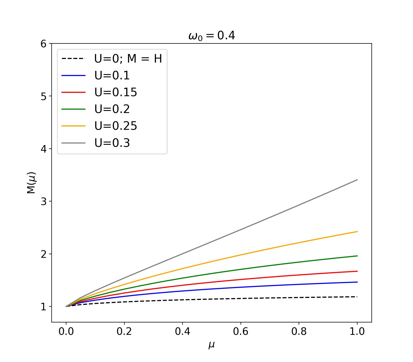
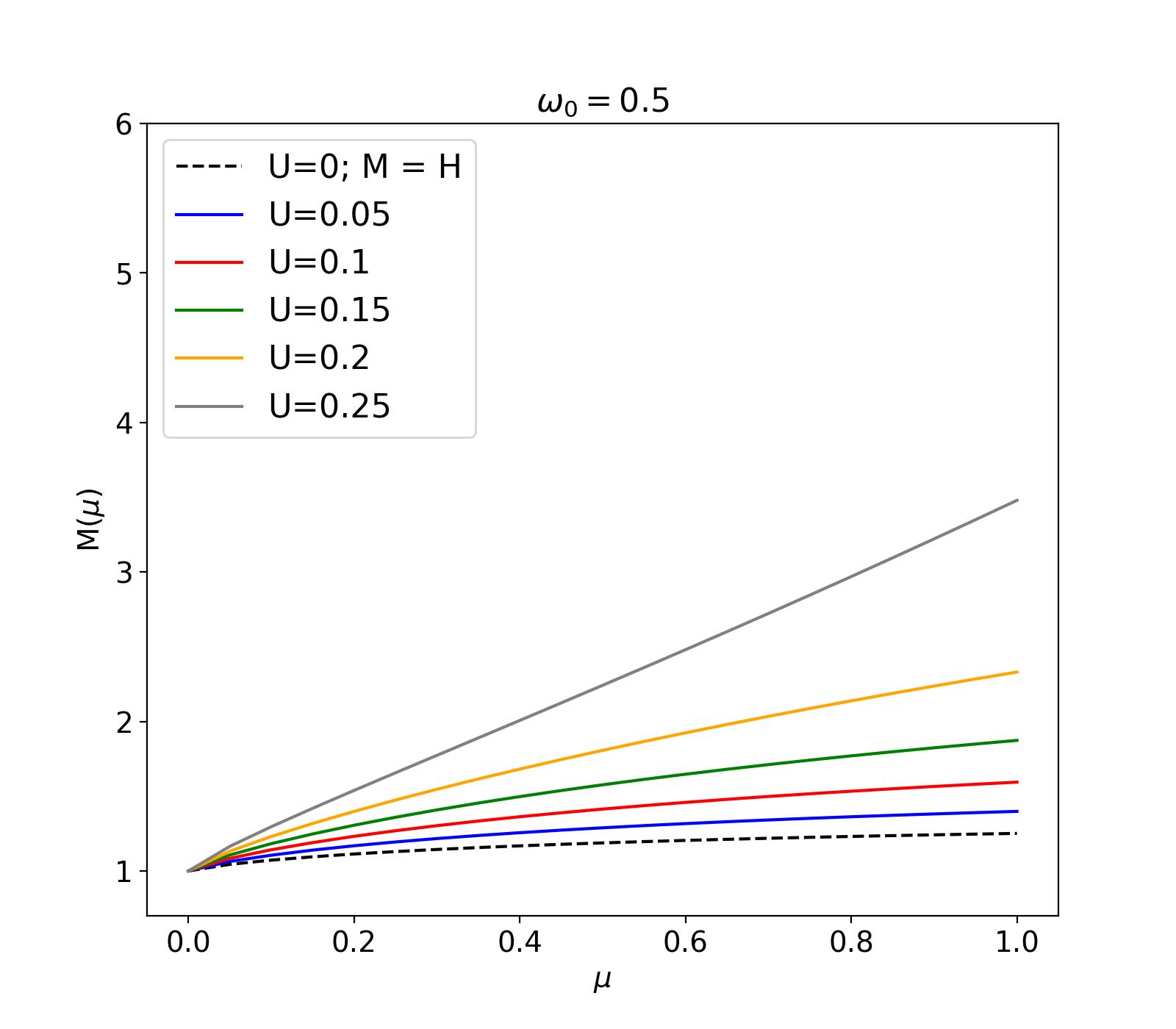
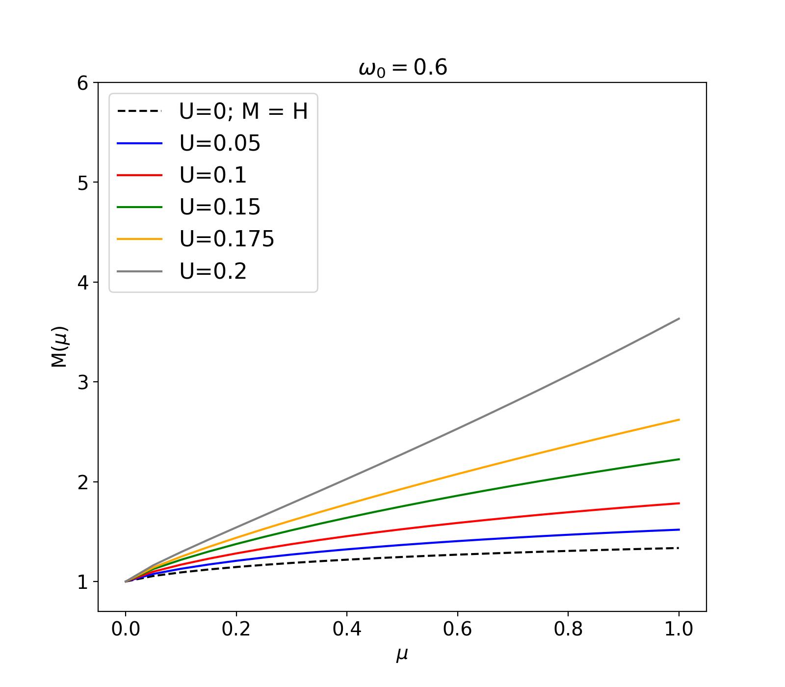
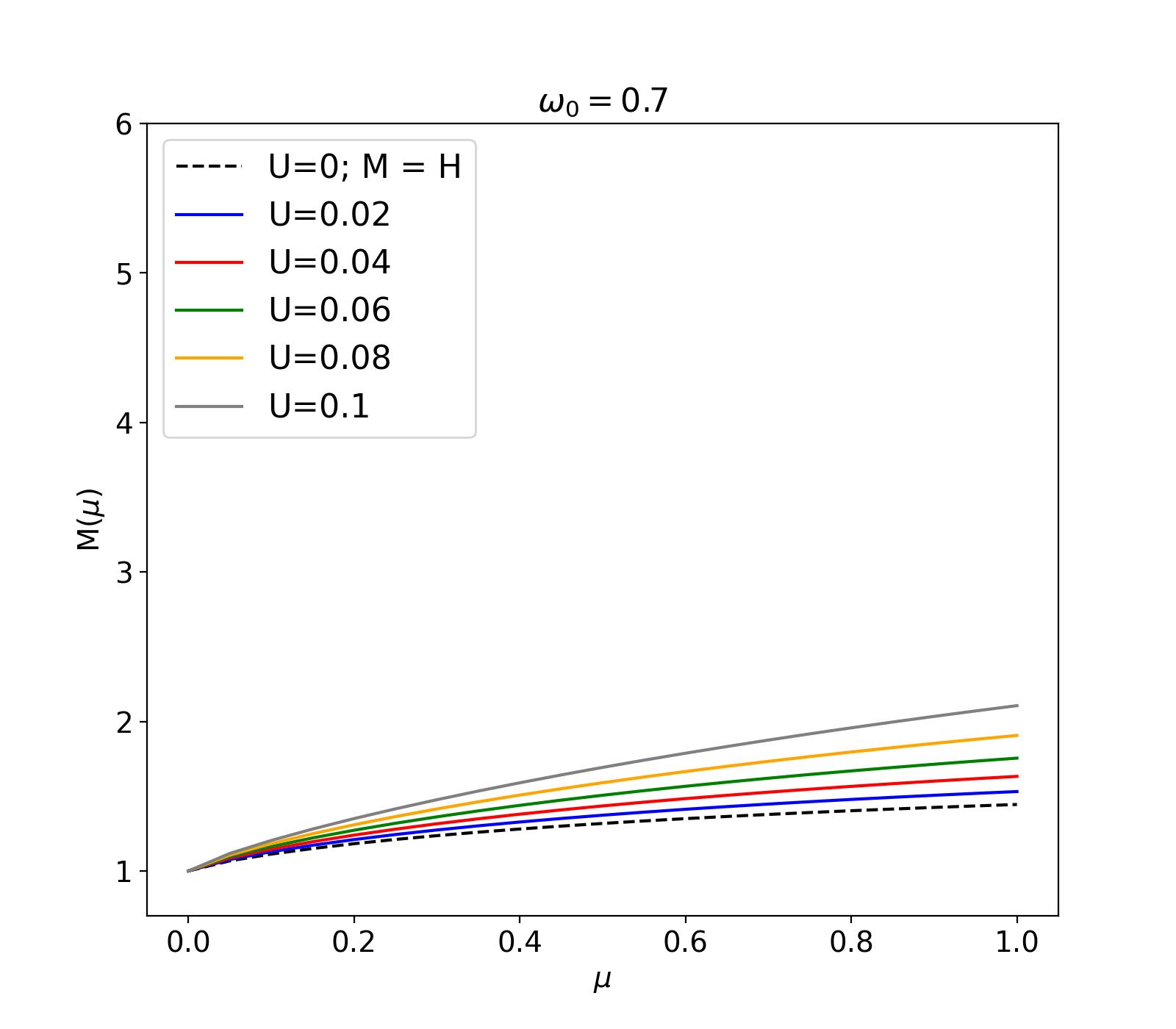
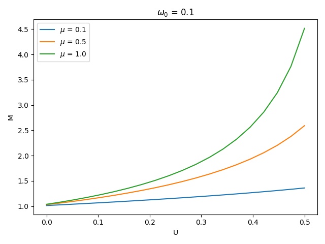
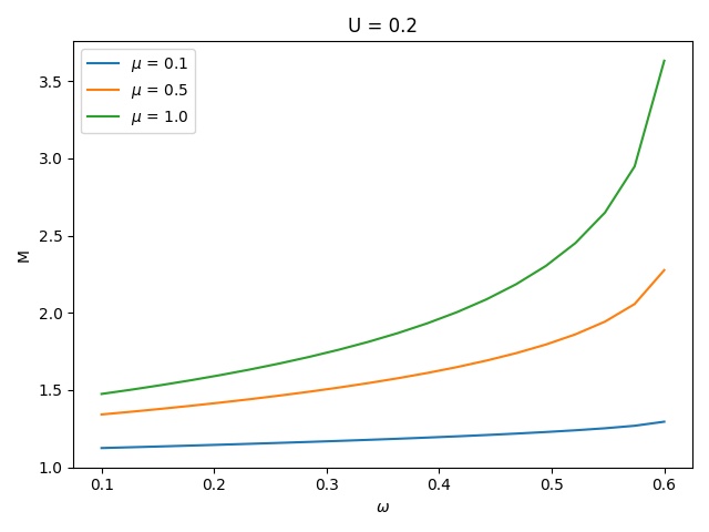
Finally, we considered the most general case where both scattering and thermal emission occur simultaneously () sec(3.3). When comparing different values of , we observe that increases with U for fixed as shown in fig. 2. The same is true for fixed U and increasing as shown in fig.3. This shows a nonlinear interplay between and , where higher scattering albedo increases the scattering of thermally emitted photons, thereby enhancing the overall reflected intensity. Physically for higher U, more number of plank photons are generated during emission. Now for higher this photons are scattered more and enhance the final radiation. Hence, the thermal emission and scattering create a feedback loop that amplifies the total radiation. Hence both the effect of scattering and emission plays crucial role in case of semi-infinite diffuse reflection.
In particular, at (i.e., grazing angle to the surface), the and functions converge to 1, irrespective of the values of or . This indicates that at grazing angles, the effects of thermal emission and scattering cannot be distinguished. With increasing U the value of M does not vary for the tangential direction . However, the difference between these two functions becomes most pronounced at the normal angle (), as expected from the behavior of thermal emission and scattering at different angles. Hence the effect of thermal emission is more prominent along the normal direction of the scattering layer.
Figure.3 also replicates the similar trend in terms of the single scattering albedo . The scattering is much more effective along the normal direction of the plane. Also with the increasing U the separation between each curves increases due to the addition of more plank photons.
As a whole the is monotonically increasing with all of its parameters see figure 1. These findings underline the complex interactions between scattering and thermal emission in determining the reflected specific intensity, especially in cases with high scattering albedo and thermal emission coefficients. They also provide a foundation for the calculation of radiative transfer in atmospheres where both processes are significant.
Thus, we can conclude that the function, incorporating both isotropic scattering and thermal emission, is a more generalized version of Chandrasekhar’s function. This result expands the applicability of Chandrasekhar’s work by including the effect of thermal emission in the radiative transfer equation. The consistency between and (see sec. 4) in the appropriate limit ensures that our formulation retains the well-established behaviors in the absence of thermal emission while providing a more comprehensive description when emission is present.
5.4 Limitations and Future work
This work is the first attempt to quantitatively establish the thermal emission contribution for the semi-infinite diffuse reflection problem for the isotropic scattering case. While this work presents a comprehensive analysis of the function, there are a few limitations that should be highlighted, which can be addressed in future research.
Firstly, we have treated the thermal emission coefficient as a variable parameter rather than explicitly incorporating temperature as a direct variable. Although this approach is effective for many practical applications, especially in cases where temperature gradients are less significant, a more detailed analysis where temperature is modeled explicitly could provide a more accurate representation in systems with complex temperature profiles, where temperature dependencies significantly influence the radiative transfer.
Secondly, in the conservative case of perfect scattering, where , numerical solutions for the function were achieved only for U=0 case within the parameter range considered in this study. In this limit, thermal emission becomes impossible, and the system reduces to the purely scattering case, which is well understood in the literature. However, further work could explore methods for addressing this specific case and ensure smooth transitions between scattering and thermal emission regimes, enhancing the flexibility of the model for various astrophysical environments.
Despite these limitations, this work provides a solid foundation for the calculation of the function, with numerous opportunities for refinement. These challenges offer pathways for future investigations, including incorporating temperature dependencies and handling the extreme limits of perfect scattering, which would further extend the applicability of our model in diverse astrophysical and planetary contexts.
One promising direction is the extension of this framework to more complex atmospheric scenarios. Specifically, the function, derived for the semi-infinite atmosphere, has a direct counterpart in the function, which is applicable to finite atmospheres as shown in Sengupta (2022). Following the approach outlined in this study, the function can also be derived and calculated for various cases of isotropic scattering and thermal emission. This would enable a more comprehensive treatment of radiative transfer in both finite and semi-infinite atmospheric contexts, providing greater applicability to a range of astrophysical environments.
In the realm of exoplanetary science, atmospheric spectra for various exoplanets, particularly Hot Jupiter-type planets, have been modeled to match observational data, including reflection, transmission, and emission spectra Tinetti et al. (2013). For such planets, incorporating the thermal emission contribution in the form of the function is crucial. The exoplanetary atmosphere is modeled directly using the function considering only the scattering phenomena Madhusudhan & Burrows (2012). Extending the present work to model the atmospheric emission spectra of exoplanets during the secondary eclipse (Hansen, 2008), accounting for both scattering and thermal emission, would enhance our ability to interpret observed data and improve our understanding of the atmospheric composition and dynamics of these distant worlds.
Additionally, the study of tidally locked gas giants offers another exciting area for future exploration. These planets experience significant day-night temperature contrasts, which influence atmospheric circulation patterns and heat redistribution. The thermal emission spectra of such planets, when combined with the scattering effects considered here, could provide deeper insights into their atmospheric structure and behavior. Studies of this nature would benefit from the inclusion of the function in models of planetary emission spectra, as discussed in Sengupta & Sengupta (2023). The interplay between emission and scattering in tidally locked exoplanets represents a complex yet fascinating avenue for further research, with important implications for the habitability of these distant worlds.
5.5 Applicability in case of exoplanetary system
In this work, we find that the contribution of thermal emission becomes significant depending on the dimensionless parameter , defined as , where is the Planck function and is the incident flux. Here we have studied an example case for exoplanetary atmosphere to apply our theory. For an exoplanetary atmosphere, the incident stellar flux at a given wavelength can be approximated by
| (26) |
where , and denote the stellar temperature, stellar radius, and the star–planet separation, respectively Guillot (2010). Assuming both the star and the planet behave as blackbodies, the planetary thermal emission at the same wavelength can be written as , where is the planet’s equilibrium temperature. The thermal emission coefficient at that wavelength is then given by
| (27) |
In this study, we have shown that the coupled emission and scattering regime is physically meaningful only for values of , within which the function converges. Moreover, the larger the value of within this convergence range, the more pronounced the thermal emission effect along with scattering.
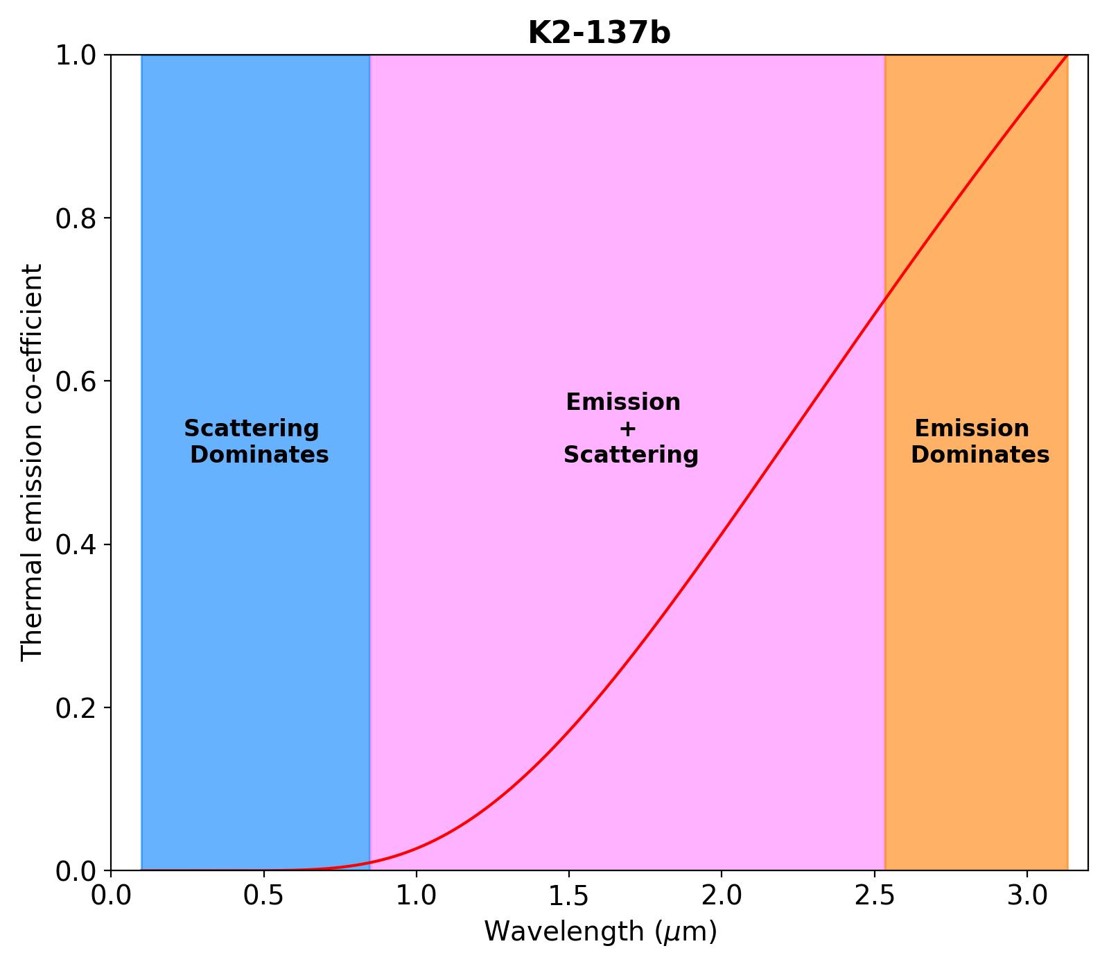
As a case study, we consider the exoplanet K2-137b, an Earth-sized planet orbiting an M-dwarf star. The parameters are as follows: , , , and orbital distance , as reported in Smith et al. (2018). Incorporating this system parameters we compute and plot Fig. 4 which shows the variation of the thermal emission coefficient as a function of wavelength for the ultra-short-period exoplanet K2-137b, assuming blackbody spectra for both the planet and its host M-dwarf star. The resulting curve demonstrates a monotonic increase in with wavelength.
Three distinct radiative regimes are indicated in the plot:
-
•
Scattering-dominated regime (, shaded blue): Here, , implying that the incoming stellar irradiation dominates the radiative budget. The thermal emission from the planet is negligible, and the radiative transfer is governed primarily by scattering processes. In this region the diffuse reflection theory of Chandrasekhar (1960) can be used without any modification.
-
•
Simultaneous emission–scattering regime (, shaded pink): This region corresponds to , where both thermal emission and scattering contribute significantly. Within this range, the function has been shown to converge, marking it as the valid regime for the theoretical model of coupled emission and scattering proposed in Sengupta (2021, 2022) and developed in this work.
-
•
Emission-dominated regime (, shaded orange): In this domain, , suggesting that thermal emission dominates the radiative transfer. The diverging in this region, and the radiative transfer is dominated by emission. Hence diffuse reflection theory loses it’s meaning and applicabilty in the region and further.
The spectral window between and is thus identified as the optimal regime for validating the theoretical framework under conditions where both scattering and emission are relevant. In the observational prospect, several instruments like JWST-NIRSpec, HST-WFC3, ARIEL enable potential empirical validation of the emission–scattering model across a range of hot exoplanets, with K2-137b serving as a promising initial candidate. A comprehensive statistical study, observational sensitivity for multiple exoplanets, however, is out of the scope of the present article and left for future work.
6 Conclusion
The theorems and values presented here offer a robust mathematical framework for modeling radiative transfer in atmospheres where both scattering and thermal emission play significant roles. This is particularly important for astrophysical phenomena involving exoplanets, Hot Jupiters, and brown dwarfs, where both thermal emission and scattering contribute comparably to the final emergent radiation. Our results directly address the need for accurate modeling of the reflected specific intensity in such systems, which is crucial for interpreting transmission and reflection spectra from observational data.
Moreover, the ability to quantify the function and its moments opens the door for more precise predictions of radiative properties in thermally active atmospheres. This is expected to have important implications for the study of habitability, energy balance, and atmospheric composition in exoplanet research, as well as for more general applications in planetary science and astrophysics. Overall, these potential research directions open new opportunities to refine and expand upon the current understanding of radiative transfer in astrophysical and planetary atmospheres. By addressing these complex cases and incorporating additional physical processes, future studies can provide a more holistic view of the radiative properties of exoplanets and other celestial bodies. In conclusion, the theorems developed in this work provide a comprehensive, generalized framework for understanding radiative transfer in semi-infinite atmospheres with both scattering and thermal emission, making a significant contribution to the field of radiative transfer theory and its applications in astrophysics and beyond.
Appendix A Alternate proof of the zeroth moment
Here we present an alternate way to prof corollary 1.3. This method is more direct than that presented in the main text.
Proof.
For n=0, eqn.(3) can be represented as,
| (A1) |
Switching and in the last expression and taking average we will get,
| (A2) |
Now this quadratic equation has the following possible solutions,
References
- Anlı & Öztürk (2021) Anlı, F., & Öztürk, H. 2021, Journal of Quantitative Spectroscopy and Radiative Transfer, 272, 107764
- Batygin & Stevenson (2010) Batygin, K., & Stevenson, D. J. 2010, The Astrophysical Journal Letters, 714, L238
- Bellman et al. (1967) Bellman, R., Kagiwada, H., Kalaba, R., & Ueno, S. 1967, Icarus, 7, 365
- Bosma & De Rooij (1983) Bosma, P., & De Rooij, W. 1983, Astronomy and Astrophysics (ISSN 0004-6361), vol. 126, no. 2, Oct. 1983, p. 283-292., 126, 283
- Chandrasekhar (1947) Chandrasekhar, S. 1947, The Astrophysical Journal, 105, 164
- Chandrasekhar (1960) —. 1960, Radiative Transfer, Dover Books on Intermediate and Advanced Mathematics (Dover Publications). https://books.google.co.in/books?id=CK3HDRwCT5YC
- Chandrasekhar & Breen (1947) Chandrasekhar, S., & Breen, F. H. 1947, The Astrophysical Journal, 106, 143
- Chandrasekhar & Breen (1948) —. 1948, Astrophysical Journal, 107, 216
- Das & Bera (2007) Das, R. N., & Bera, R. 2007, arXiv preprint arXiv:0711.3336
- Dubus et al. (1986) Dubus, A., Devooght, J., & Dehaes, J.-C. 1986, Nuclear Instruments and Methods in Physics Research Section B: Beam Interactions with Materials and Atoms, 13, 623
- Guillot (2010) Guillot, T. 2010, Astronomy & Astrophysics, 520, A27
- Hansen (2008) Hansen, B. M. 2008, The Astrophysical Journal Supplement Series, 179, 484
- Jablonski (2015) Jablonski, A. 2015, Computer Physics Communications, 196, 416
- Jablonski (2019) —. 2019, Computer Physics Communications, 235, 489
- Komacek & Youdin (2017) Komacek, T. D., & Youdin, A. N. 2017, The Astrophysical Journal, 844, 94
- Madhusudhan & Burrows (2012) Madhusudhan, N., & Burrows, A. 2012, The Astrophysical Journal, 747, 25
- Mihalas (1978) Mihalas, D. 1978, San Francisco: WH Freeman
- Sengupta (2021) Sengupta, S. 2021, The Astrophysical Journal, 911, 126
- Sengupta (2022) —. 2022, The Astrophysical Journal, 936, 139
- Sengupta & Sengupta (2023) Sengupta, S., & Sengupta, S. 2023, New Astronomy, 100, 101987
- Singla et al. (2023) Singla, M., Chakrabarty, A., & Sengupta, S. 2023, The Astrophysical Journal, 944, 155
- Singla & Sengupta (2023) Singla, M., & Sengupta, S. 2023, New Astronomy, 102, 102024
- Smith et al. (2018) Smith, A., Cabrera, J., Csizmadia, S., et al. 2018, Monthly Notices of the Royal Astronomical Society, 474, 5523
- Tinetti et al. (2013) Tinetti, G., Encrenaz, T., & Coustenis, A. 2013, The Astronomy and Astrophysics Review, 21, 1