Linear Convergence of Plug-and-Play Algorithms with Kernel Denoisers
Abstract
The use of denoisers for image reconstruction has shown significant potential, especially for the Plug-and-Play (PnP) framework. In PnP, a powerful denoiser is used as an implicit regularizer in proximal algorithms such as ISTA and ADMM. The focus of this work is on the convergence of PnP iterates for linear inverse problems using kernel denoisers. It was shown in prior work that the update operator in standard PnP is contractive for symmetric kernel denoisers under appropriate conditions on the denoiser and the linear forward operator. Consequently, we could establish global linear convergence of the iterates using the contraction mapping theorem. In this work, we develop a unified framework to establish global linear convergence for symmetric and nonsymmetric kernel denoisers. Additionally, we derive quantitative bounds on the contraction factor (convergence rate) for inpainting, deblurring, and superresolution. We present numerical results to validate our theoretical findings.
Index Terms:
image regularization, plug-and-play, kernel denoiser, contraction mapping, linear convergence.I Introduction
The use of denoisers for iterative image reconstruction was pioneered by the seminal works [1, 2], where classical image denoisers such as NLM [3] and BM3D [4] were used for image reconstruction. Later, it was shown that one could get state-of-the-art reconstructions using trained denoisers [5, 6]. Thus, PnP enables the integration of deep image priors with model-based inversion [7]. However, it is also known that standard pretrained denoisers, such as DnCNN [8], may cause the reconstruction process to diverge [9, 10, 11]. Consequently, providing theoretical guarantees for such denoisers is challenging and often requires redesigning or retraining the network [12, 11, 13, 14, 15, 16, 17, 18, 19, 20, 21, 22, 23, 24].
In this work, we revisit the Plug-and-Play (PnP) method [2], where regularization is performed by replacing the proximal operator in algorithms such as ISTA and ADMM [25] with an off-the-shelf denoiser. More specifically, consider the problem of recovering an image from linear measurements
| (1) |
where is the forward operator, is the observed image, and is white Gaussian noise. The standard inversion framework involves the loss function
| (2) |
and a convex regularizer . The reconstruction is performed by considering the optimization problem
| (3) |
and solving it iteratively using proximal algorithms [25, 26]. For example, starting with , the updates in ISTA are given by
| (4) |
where is the step size and is the proximal operator of [26],
| (5) |
We can alternatively solve (3) using ADMM, which is known to exhibit better empirical convergence [25]. Starting with and some fixed parameter , the updates in ADMM are given by
| (6) | ||||
Both ISTA and ADMM are known to converge to a minimizer of (3) under mild technical assumptions [26, 27].
I-A PnP algorithms
PnP is founded on a simple yet profound insight: rather than explicitly defining the regularizer and computing its proximal operator in (4) and (I), one can directly replace the proximal operator with a powerful denoiser. After all, the proximal operator of inherently serves as a denoising mechanism in these algorithms. More specifically, we perform the update as
| (7) |
where in (4) is replaced by a denoising operator . This is referred to as PnP-ISTA. Similarly, in the PnP variant of (I), called PnP-ADMM, the updates are performed as follows:
| (8) | ||||
As suggested by the notation in (7) and (I-A), our focus is on the use of linear denoisers for , such as NLM [3], LARK [28], DSG-NLM [2], and GLIDE [29]. This combination of linear inverse problems and linear denoisers is the simplest PnP model that works well in practice [2, 10, 30] and is analytically tractable [31, 32, 17]. A detailed discussion of linear denoisers is provided in Section II-A.
PnP gives state-of-the-art results with trained denoisers [8, 6, 13, 33]. However, from an operator-theoretic perspective, it is not immediately clear why the sequence generated by (7) should converge, let alone produce good results, unless the trained denoiser is proximable or an averaged operator [34]. In particular, it has been shown that trained denoisers can result in divergence of the PnP iterations [9, 11, 35] and, thus, a convergence guarantee can act as a safeguard. The convergence aspect of PnP is an active area of research [12, 11, 13, 14, 17, 18, 19].
In this paper, we complete the work started in [31], where it is shown that PnP-ISTA iterates converge linearly for symmetric denoisers [2, 29, 36]. This is based on the observation that (7) can be viewed as a fixed-point iteration , where the update operator is derived from the forward and denoising operators and . Similarly, the iterates in (I-A) can be written as , where is given by the fixed-point iteration , and is again derived from and . The main result in [31] is that if is a symmetric denoiser and corresponds to inpainting, deblurring, or superresolution, then and are contractive for any and (see Section II-B). Subsequently, the contraction mapping theorem [34] was used to guarantee global linear convergence of (7) and (I-A) to a unique reconstruction. Notably, the contractivity of and was deduced from niche properties of such as positive semidefiniteness and irreducibility.
I-B Contributions
The present work is motivated by the question of whether the results in [31] can be extended to a broader range of kernel denoisers, such as NLM [3], which are neither symmetric nor nonexpansive with respect to the standard Euclidean inner product, but are faster than their symmetric counterparts [2]. Our main results are as follows.
-
1.
We present a counterexample to show that the update operator in PnP-ISTA is generally not contractive if is nonsymmetric, i.e., the analysis in [31] cannot directly be extended to kernel denoisers, even if we work with a different norm.
-
2.
Subsequently, motivated by prior work [17], we consider scaled variants of PnP-ISTA and PnP-ADMM for (nonsymmetric) kernel denoisers and prove that the respective update operators are contractive. However, the contractivity in question is not w.r.t. the Euclidean norm but w.r.t. a quadratic norm derived from . This way, we can extend the linear convergence guarantee in [31] from symmetric denoisers to nonsymmetric denoisers. In particular, we develop a unified convergence theory for symmetric and nonsymmetric denoisers.
-
3.
We derive bounds on the contraction factor in terms of problem parameters such as the subsampling rate, the spectral gap of , and parameters and . It turns out that the actual contraction factors are barely less than , and a delicate analysis is required to compute bounds that are strictly less than . In particular, we study the effect of various measurement and algorithmic parameters on the actual and estimated contraction factors.
I-C Organization
In Sec. II, we provide the necessary background on kernel denoisers and discuss our prior work. We motivate the problem and discuss scaled PnP algorithms that go naturally with kernel denoisers in Sec. III. We present our main results in Sections IV and V, which are numerically validated in Sec. VI.
I-D Notation
We denote the all-ones vector in by . The spectrum and the spectral norm of are denoted by and . We use to denote the space of symmetric matrices and to denote the set of symmetric positive semidefinite matrices. We use to denote the fixed points of , i.e., . For any , we use to represent a diagonal matrix with as its diagonal elements; additionally, we use to denote the vector consisting of the diagonal elements of . We use if and are similar. Unless stated otherwise, we denote an abstract inner product on as and the associated norm as . In particular, we use for the dot product on and for the corresponding norm.
II Background
II-A Kernel denoiser
A kernel denoiser is abstractly a linear transform that takes a noisy image and returns the denoised output. More precisely, let be the input image, where is a finite square grid, and let be the intensity value at location . A kernel denoiser is specified using a kernel function , where measures the affinity between pixels [36]. The denoiser output is given by
| (9) |
In other words, the output at a given pixel is obtained using a weighted average of neighboring pixels, where the weights are derived from the affinity between pixels.
From (9), it is clear that is a linear operator on a finite-dimensional vector space. Hence, it is convenient to express (9) in matrix form. More precisely, if we linearly index and let be the vector representation of corresponding to this indexing, we can represent (9) as
| (10) |
where is called the kernel matrix. We refer the reader to [36] for a detailed account of this class of denoisers. Apart from denoising [3, 28, 30, 37], kernel denoisers have also been used for graph signal processing [38, 39].
We note that there are subtle variations across the literature in the definition of for NLM [2, 3, 40]. These variations do not significantly impact the denoising performance but can affect the mathematical properties. To avoid confusion, we explicitly state the properties required for our analysis.
Assumption 1.
The kernel matrix has these properties:
-
1.
.
-
2.
is nonnegative and irreducible.
-
3.
for .
In particular, since is nonnegative and , . Thus, is invertible, which is implicitly used in (10).
A commonly used example of a kernel function in the literature is
| (11) |
where is an isotropic multivariate Gaussian with standard deviation , is a patch around extracted from a guide image, and is a hat function supported on a square window around the origin ( is used to restrict the averaging to a local window). The guide is the input image or some surrogate of the ground truth estimated from the observed image.
For the kernel in (11), we can verify that the corresponding follows Assumption 1. Clearly, is symmetric, nonnegative, and in this case. Furthermore, we can show that is irreducible if . Indeed, this follows from the path-based characterization of irreducibility [41]: for any two pixels , we can find a sequence of pixels such that for . On the other hand, the property is more subtle; this property is not guaranteed if a box function is used in place of , as done in the standard setting [3]. That follows from Bochner’s theorem [42], and we refer the reader to [2, Appendix B] for a detailed explanation. In short, both and are positive definite functions since they are the Fourier transforms of nonnegative functions. Consequently, the corresponding kernel matrices and are positive semidefinite, and thus their Hadamard product is also positive semidefinite.
As a consequence of Assumption 1, we have the following structure on .
Proposition 1.
If Assumption 1 holds, then
-
(1)
is nonnegative and irreducible. (Perron matrix)
-
(2)
. (stochastic matrix)
-
(3)
Eigenvalues of are .
Properties (1) and (2) follow from the properties of and the fact that . To deduce (3), we write (10) as
Since , where , the eigenvalues of must be nonnegative. Furthermore, it follows from (1) and (2) that and that is its largest eigenvalue. In fact, since is a Perron matrix, it follows from the Perron-Frobenius theorem [41] that . The difference , which will play an important role in our analysis, is called the “spectral gap”. This is related to the connectivity of the graph associated with : the spectral gap is nonzero if and only if the graph is connected, and the gap increases with the connectivity [43].
Note that while and are symmetric, in (10) does not necessarily have to be symmetric. Specifically, while is row-stochastic, it is generally not doubly stochastic. This class of denoisers includes NLM [3] and LARK [28], which we call kernel denoisers in this paper. On the other hand, denoisers such as GLIDE [29] and DSG-NLM [2] have the additional property that is symmetric, and their definitions differ from (10). In particular, the DSG-NLM protocol from [2, Section IV] can be applied to any kernel denoiser to obtain a symmetric that satisfies the properties in Proposition 1. We will refer to them as symmetric denoisers to distinguish them from kernel denoisers.
Remark 1.
A natural question is whether the standard analysis of ISTA can be directly applied to PnP-ISTA. Indeed, this approach was taken in the original PnP paper [2]. However, this method applies only to symmetric denoisers that are proximable [44, 45], i.e., the denoiser is the proximal operator of some convex function. Since kernel denoisers are generally non-symmetric, they are not proximable, and therefore, the convergence analysis in [2] does not extend to them. Additionally, this has to do with objective convergence, which is generally weaker than iterate convergence––the focus of the present work. In this regard, we note that Krasnosel’skii-Mann (KM) theory [34] can establish iterate convergence of ISTA. However, KM theory applies to PnP-ISTA only if the denoiser is proximable or, more generally, an averaged operator. As we will show later, a kernel denoiser may fail to be nonexpansive and, consequently, cannot be an averaged operator, given that averaged operators are necessarily nonexpansive. In summary, ensuring objective and iterate convergence for kernel denoisers is challenging. We can establish both forms of convergence for symmetric denoisers, but we cannot generally guarantee linear convergence as done in this work.
II-B Prior work
It was shown in [31] that PnP-ISTA converges linearly if is a symmetric denoiser. This is based on the observation that on substituting (2) in (7), we get
| (12) |
where
| (13) |
That is, we can write (12) as the fixed-point iteration , where . In particular, is a contraction if . In this regard, we recall the following result [31].
Theorem 1.
If is a symmetric denoiser and , then for inpainting, deblurring, and superresolution.
Consequently, it follows from the contraction mapping theorem [34, Thm. 1.48] that converges linearly to a unique reconstruction for any initialization . In other words, PnP-ISTA is guaranteed to converge globally at a geometric rate for inpainting, deblurring, and superresolution. A similar result was also derived for PnP-ADMM in [31].
Thm. 1 is a nontrivial observation since and are not contractive w.r.t. the spectral norm. Indeed, from Prop. 1, and since has a nontrivial nullspace for inpainting, deblurring, and superresolution. Thm. 1 can be deduced using a subtle relation between the eigenspaces of these operators.
We remark that the irreducibility property in Assumption 1 is crucial for Theorem 1. For example, (though not corresponding to a practical denoiser) satisfies all the properties in Proposition 1 except irreducibility. In this case, , so that any nonzero vector in the null space of is a fixed point of . Consequently, cannot be a contraction operator.
A natural question is whether Thm. 1 can be extended to a kernel denoiser. It was empirically observed in [31, Table 1] that for kernel denoisers. This is essentially because of the nonsymmetry of . Indeed, consider the setting , corresponding to having full measurements. In this case, and . Now, consider a kernel denoiser that is not doubly stochastic, i.e., while the row sums equal one, the column sums do not. We can show that for such a denoiser. Subsequently, we have for . That is, no matter how small is, we can construct a kernel denoiser and for which for some in . However, this example does not eliminate the possibility that may be contractive in a different norm.
As an exception, it was shown in [31] that linear convergence can be established for inpainting with kernel denoisers. The key idea was to establish contractivity of in a different operator norm. Specifically, consider the operator norm
| (14) |
induced by the following inner product and norm on :
| (15) |
where is given by (10). We will refer to (14) as the -norm. The following is a restatement of [31, Thm. 3].
Theorem 2.
If is a kernel denoiser and , then for inpainting.
II-C A counterexample
Thm. 2 strongly relies on the diagonal nature of for inpainting and cannot be extended to deblurring and superresolution. Using a concrete deblurring example, we will prove that cannot be guaranteed with a kernel denoiser. Consider the forward operator corresponding to a uniform blur. Consider a hypothetical case where the pixel (and patch) values are and ; this is modeled on the pixel distribution near an edge. For any , consider the kernel matrix given by
We can verify that satisfies Assumption 1 for all . The only nontrivial property is ; this comes from Bochner’s theorem [42] as is the Fourier transform of a nonnegative function.
Let and be obtained by letting in (10), so that has the properties in Prop. 1. Since working directly with and is difficult, we consider their limiting forms:
| (16) |
and
| (17) |
where is the all-ones matrix. If we let , then
| (18) |
Moreover, we can show from (16) and (17) that
The quantity on the right is strictly greater than for all . Hence, using the continuity of norm and (18), we can conclude that, for all , for some . While the above counterexample is somewhat artificial, it tells us that the contractivity of cannot generally be guaranteed for deburring using the -norm.
III PnP with Kernel Denoisers
We now explain how iterate convergence of PnP with kernel denoisers can be established. To this end, we consider the class of scaled PnP algorithms introduced in [17]. This work demonstrated that rather than symmetrizing the denoiser using the DSG-NLM protocol—which increases the computational cost–the diagonalizability of kernel denoisers can be leveraged to make them self-adjoint with respect to a special inner product. This requires us to use a slightly modified version of the original PnP algorithm called scaled PnP. In particular, this insight allowed us to interpret a kernel denoiser as a proximal operator, which helped establish objective convergence for scaled PnP [17]. In the following sections, we will develop a common framework to analyze the iterates of ISTA generated by a kernel denoiser that satisfies the properties outlined in Prop. 1, regardless of whether it is symmetric or nonsymmetric. We will use this framework to demonstrate the global linear convergence of the iterates and estimate the convergence rates.
To explain the motivation behind scaled PnP, we observe that although (10) is nonsymmetric, it is self-adjoint w.r.t. the inner product defined in (15). That is, for all ,
Thus, while a symmetric denoiser is self-adjoint w.r.t. the standard dot product on , a kernel denoiser is self-adjoint w.r.t. the inner product (15). This suggests that working in the inner-product space would be more natural for kernel denoisers. This was the original motivation behind the scaled PnP algorithms in [17], which amounts to reformulating PnP-ISTA and PnP-ADMM in . In this context, we note that ISTA and ADMM can be developed in the general setting of inner-product spaces [46, 34]. The former requires us to specify the gradient, and the latter requires the proximal operator, both of which depend crucially on the choice of the inner product.
We can show from (15) that the gradient of (2) w.r.t. is , where is the standard gradient operator. As a result, the PnP-ISTA update (7) has to be corrected to
| (19) |
where is a kernel denoiser. This is referred to as Scaled PnP-ISTA (Sc-PnP-ISTA) in [17]. On substituting (2), we can write (19) as
| (20) |
where is an irrelevant vector, and
| (21) |
On the other hand, by working with the proximal operator in , we obtain the scaled counterpart of (I-A). More precisely, we need to work with
| (22) |
which is obtained by replacing in (5) with the -norm. In particular, Sc-PnP-ADMM updates are given by
| (23) | ||||
On substituting the loss (2) in (22), we get
| (24) |
where does not depend on . Importantly, we can write the iterates in (III) as
| (25) |
where is an irrelevant quantity. We refer the reader to [31, Prop. 1] for the precise definition of . This standard reduction comes from the Douglas-Rachford splitting used in ADMM [25]. Importantly, using (24), we can show that
| (26) |
where
| (27) |
Similar to (21), the operator (26) involves the composition of two linear operators, one determined by the forward model and the other by the denoiser. However, the operator in (26) is more complicated. Note that, unlike in the symmetric case, the operators and are controlled by the denoiser via .
IV Linear Convergence of PnP
As was observed in [17], we can associate Sc-PnP-ISTA and Sc-PnP-ADMM with a convex optimization problem of the form (3). Consequently, we can establish iterate convergence from standard results [46, 27]. Moreover, if the loss function (2) is strongly convex, then the iterates can converge linearly [46]. However, since has a nontrivial nullspace for linear inverse problems [7], the loss function cannot be strongly convex. At this point, we clarify what linear convergence means. A sequence is said to converge linearly if there exist , and some norm on such that
| (28) |
It follows from (20) that . Hence, if we can show that , we would have (28) with . Similarly, since for a kernel denoiser, we have from (25) that
Now, recall that . Hence, if we can show that , we would have (28) for with .
For linear inverse problems such as inpainting, deblurring, and superresolution, the forward operator is given by a mix of lowpass blur (convolution) and subsampling operations [7]. For inpainting, is a diagonal matrix with . On the other hand, is typically a Gaussian or uniform blur in image deblurring. For superresolution, , where is a subsampling operator, and is a lowpass blur. We will make the following assumptions that usually hold for such applications.
Assumption 2.
For inpainting (resp. superresolution), at least one pixel is observed (resp. sampled). The blur kernel is nonnegative and normalized for deblurring and superresolution: and .
The above properties will play an essential role in establishing contractivity. Moreover, we will use them to bound the norm of the forward operator.
Remark 2.
It follows from Assumption 2 that for inpainting, deblurring, and superresolution. In fact, for inpainting, deblurring, and for superresolution.
Consider a kernel denoiser and a forward operator that satisfies Assumption 2. Using properties listed in Prop. 1, we can show that and . However, this does not necessarily mean they are contractive. Indeed, if there exists a nonzero vector which is also a fixed point of , then we would have
so that cannot be contractive. Similarly, if is a nonzero vector in , then we have and . Consequently, , and cannot be contractive. In other words, for and to be contractive, the null space of and the fixed points of must intersect trivially. We record this property as it plays a fundamental role in our analysis.
Definition 1 (RNP).
Operator is said to have the Restricted Nullity Property w.r.t. if .
As noted earlier, typically has a nontrivial nullspace, i.e., it is possible that for some nonzero . However, if we restrict to , then RNP stipulates that .
Proposition 2.
For inpainting, deblurring, and superresolution, has RNP w.r.t symmetric and kernel denoisers.
Proof.
We have from Prop. 1 that . Thus, we are done if we can show that . Now, for inpainting, since for some , we have . Also, for deblurring, and, for superresolution, , which is the all-ones vector in . ∎
Remarkably, RNP is sufficient for and to be contractive. To establish this, we need the following result. Recall that any self-adjoint operator on an inner-product space can be diagonalized in an orthonormal basis [41]. Namely, there exists and an orthonormal basis such that for all . We also note that the operator norm of is defined as .
Lemma 1.
Let and be self-adjoint on . Suppose that and . Then .
This is an adaptation of [31, Lemma 1]. To keep the account self-contained, we provide a short proof in Appendix VII-A. The core idea behind Lemma 1 is the following observation.
Proposition 3.
Let be self-adjoint on and let . Then if and only if , where is the norm induced by .
We skip the proof which can easily be deduced from the eigendecomposition of .
Theorem 3.
Let be a kernel denoiser. Then, for any , we have for inpainting, deblurring, and superresolution and hence Sc-PnP-ISTA converges linearly.
Proof.
We now establish the contractivity of the operator in Sc-PnP-ADMM.
Theorem 4.
Let be an invertible kernel denoiser. Then, for any , we have for inpainting, deblurring, and superresolution and Sc-PnP-ADMM converges linearly.
Proof.
Note that it suffices to show that . Indeed, in this case, we have from (26) and the triangle inequality that
We apply Lemma 1 to with and . It is not difficult to show that and are self-adjoint on . Moreover, . On the other hand, we claim that , which is contained in for all . Indeed, it follows from (27) that
| (31) |
where is given by (30). However, we have already seen that , and hence our claim follows from (31).
Remark 3.
It can be shown that , and consequently , is nonsingular for NLM and DSG-NLM [47, Thm. 2.16]. Thus, and , where the latter is used in the proof of Thm. 4. However, we can show that Thm. 4 is valid even when is singular. We choose to work with this assumption since the kernel denoisers we employ are invertible, and the analysis is simplified by assuming invertibility.
Remark 4.
We note that scaled PnP does not change the loss function in (2), which arises from the linear measurement model and the Gaussian noise assumption. The only modification is in the regularization component, which is symmetrized by introducing the -inner product as discussed above.
V Contraction Factor
We have shown that the update operator in PnP-ISTA and PnP-ADMM is contractive. However, this is only a qualitative result, and ideally, we would like to derive a formula for the contraction factor. Unfortunately, deriving an exact formula is difficult, so we calculate an upper bound instead. This will allow us to understand how the convergence rate is influenced by factors such as the sampling rate, the spectral gap of , and the algorithmic parameters and . As we will see later, the contraction factor (computed numerically) is close to . Consequently, obtaining a bound that is becomes technically challenging. First, we present the following quantitative form of Lemma 1 (see Appendix VII-B for the proof).
Lemma 2.
Let and be self-adjoint on and . Let the eigenvalues of be
| (32) |
and let be a unit eigenvector corresponding to . Then
| (33) |
We can use Lemma 2 to bound the contraction factor. Given (33), we just need to bound the quantity , where is for PnP-ISTA and PnP-ADMM. In particular, the RNP property of (Prop. 2) ensures that and (Prop. 3).
Remark 5.
The bound in (33) does not change if we switch and . This is because , where denotes the adjoint of .
V-A Contraction factor for ISTA
We get similar bounds for PnP-ISTA and Sc-PnP-ISTA. We present the analysis for the latter, as it is more intricate due to the presence of the factor in .
Proposition 4.
Let and . Then
| (34) |
Proof.
Remark 6.
For the inverse problems at hand, in (34) has a precise meaning. For inpainting, , where is the fraction of observed pixels. On the other hand, for deblurring, and for superresolution, where is the subsampling rate.
We now bound the contraction factor of the update operator in Sc-PnP-ISTA.
Theorem 5.
Let be a kernel denoiser and . Then, for inpainting and superresolution,
and, for deblurring,
Proof.
Remark 7.
The bounds in Lemma 2 might not always be . However, the design of the kernel denoisers guarantees that the spectral gap remains positive, ensuring that the bound in Thm. 5 is . For ADMM, we require an additional assumption of invertibility for the denoiser ; this is because it is possible that if is singular. However, as discussed in Thm. 4, this assumption is justified, and we obtain a bound strictly less than one for both PnP-ADMM and Sc-PnP-ADMM.
Remark 8.
We can get the bound for PnP-ISTA by setting in Thm. 5. This gives
| (36) |
for deblurring, and
| (37) |
for inpainting and superresolution.
We note that (36) and (37) are smaller than the respective bounds for a kernel denoiser. We can obtain (36) and (37) directly from Lemma 2 by substituting with a symmetric denoiser. Indeed, the operator in this case is defined in (13). Setting in (33), we need to bound , where is the top eigenvector of . For deblurring, since , we have , leading to (36). Similarly, is diagonal for inpainting with elements in , and a direct calculation gives (37).
V-B Contraction factor for ADMM
Following (26) and (27), we will use and for PnP-ADMM. As observed earlier in Thm. 4, contractivity of (resp. ) follows from the contractivity (resp. ). In particular,
Thus, we will focus on bounding and . Bounding is particularly easy for inpainting ( is diagonal) and deblurring (). A direct application of Lemma 2 on requires , which has the following closed-form expression:
| (38) |
This makes it easy to compute in Lemma 2.
Recall that the bound for PnP-ISTA involves the spectral gap of . However, we have instead of in PnP-ADMM, and can have negative eigenvalues. The counterpart of the spectral gap that comes up naturally in this case is
| (39) |


Theorem 6.
Let be a symmetric denoiser and . Then
| (40) |
for deblurring, and
| (41) |
for inpainting, where is the fraction of observed pixels.
Proof.
Unfortunately, we do not have a simple expression for similar to (38) for superresolution. The situation becomes even more complicated for Sc-PnP-ADMM, where in (27) has an additional term. Specifically, there is no straightforward expression for in deblurring and superresolution. However, is diagonal for inpainting, allowing us to easily bound .
Theorem 7.
Let be a kernel denoiser. Then, for inpainting with fraction of observed pixels, we have
| (42) |
where .
We will use the following observation to bound for deblurring and superresolution.

Proposition 5.
Let be a self-adjoint operator on with . Let be an eigenvalue of with unit eigenvector . Then
We skip the proof of Prop. 5. This follows directly from the eigendecomposition of .
Theorem 8.
Let be a kernel denoiser. Then
for deblurring, and
for superresolution, where is the subsampling rate.
Proof.
We can write
| (43) |
Note that is self-adjoint on and its eigenvalues are nonnegative. In particular, is an eigenvalue of , i.e., there exists such that . We also need the fact that . This is because
From (43), we have , where . Applying Prop. 5 with and , we get
| (44) |
Recall that we need to bound , where . Since and , it follows from (44) that
Since (and hence ) has nonnegative components (Assumption 2), we can show , where ; see [41, Sec. 8.3] for example. Moreover, as and , we have . Hence,
On the other hand,
Consequently, we have from Remark 6 that
Combining this with Lemma 2, we get the desired bounds. ∎
V-C Discussion
We remark that the bounds in Lemma 2 need not be strictly less than one. However, as the spectral gap is positive for a kernel denoiser, the bound in Thm. 5 is guaranteed to be . For ADMM, we assumed that the denoiser is invertible, which forces the spectral gap in (39) to be . However, as discussed in Remark 3, NLM and DSG-NLM denoisers can be proven to be invertible, and the bound is for both PnP-ADMM and Sc-PnP-ADMM.
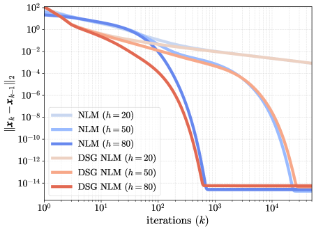
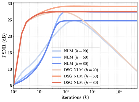
Our analysis reveals that the contraction factor decreases for both inpainting and superresolution as increases. This leads to the intuitive conclusion that convergence is faster with more measurements. It is also worth noting that, for PnP-ISTA, the bound depends on through its second-largest eigenvalue . If we view the kernel matrix as the adjacency matrix of a graph with the pixels as nodes, then (the spectral gap) represents the connectivity of the graph, indicating how quickly pixels are mixed (or diffused) through repeated applications of [40]. Better connectivity results in a smaller and faster convergence. As shown in Figs. 8 and 8 in the next section, reducing and by increasing the bandwidth can accelerate convergence. However, while a higher bandwidth improves mixing and speeds up convergence, it can also introduce excessive blurring in the reconstruction (Fig. 9). Thus, there is an optimal tradeoff between convergence speed and reconstruction accuracy.
VI Numerical Experiments
We present numerical results111The codes are available at github.com/arghyasinha/tsp-kernel-denoiser. to validate our key results, specifically Thms. 5, 6, and 8. Moreover, we wish to investigate the dependence of the contraction factor––which controls the convergence rate––on the following factors: the second eigenvalue of for PnP-ISTA, the second dominant eigenvalue of for PnP-ADMM, the fraction of observed pixels for inpainting, and the downsampling rate for superresolution. It is important to note that these experiments are not intended to assess the reconstruction accuracy of PnP-ISTA and PnP-ADMM with kernel denoisers, nor to compare them with trained denoisers; for such comparisons, we refer to [10, 30, 2, 48]. Instead, we aim to provide numerical evidence supporting the theoretical findings.
Before proceeding with the result, we discuss the computation of , the largest singular value of the update operator in ISTA. Since and are too large to be manipulated as matrices, we cannot store as a matrix and use a direct method for finding . Instead, we treat them as operators (or black boxes) and use the power method [49]. Similarly, we use the power method to compute , , and . Before applying the power method to the scaled variants and , we performed an additional step of changing the norm from to using (15). To compute the second eigenvalue , we applied the power method to the deflated operator . This approach is effective because is the leading eigenvalue of , with a one-dimensional eigenspace spanned by (see Prop. 1). Consequently, the deflated operator has as its dominant eigenvalue. Similarly, we computed using the deflated operator .
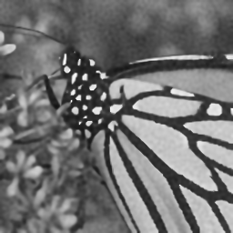
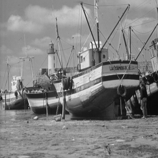
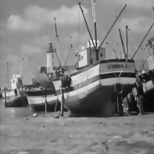
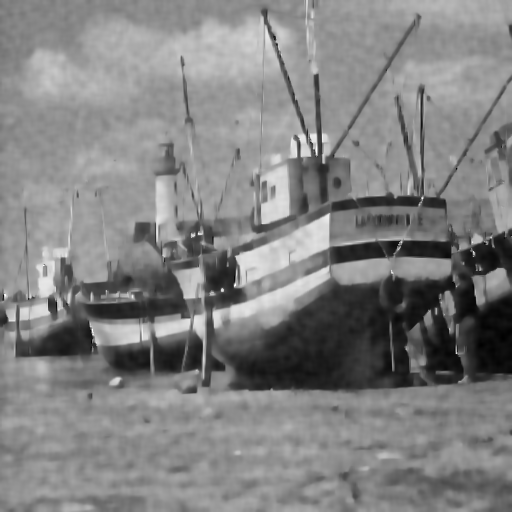
We perform inpainting, deblurring, and superresolution experiments. Unless stated otherwise, the forward operator corresponds to randomly sampling pixels for inpainting, and a Gaussian blur with standard deviation for deblurring. For superresolution, , where we take is a uniform blur and coresponds to downsampling. As for the denoiser, we consider the nonsymmetric NLM and the symmetric DSG-NLM denoisers discussed in Sec. II-A. Specifically, the key parameter in our experiments is the bandwidth (refer to Sec. II-A), the standard deviation of the underlying isotropic Gaussian kernel used in these denoisers.
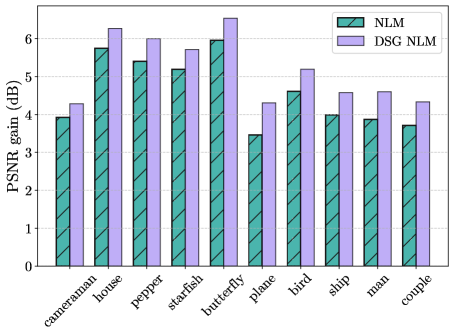
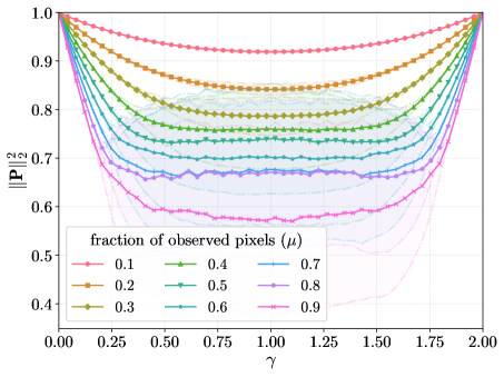
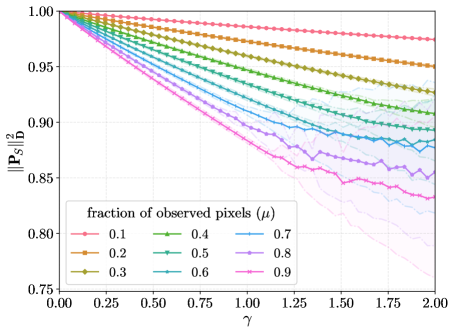
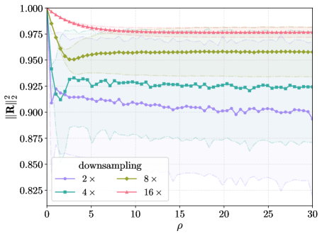
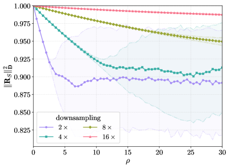
We present deblurring and superresolution results using PnP-ISTA and Sc-PnP-ISTA in Figs. 1 and 2. Additionally, in Fig. 3, we compare reconstruction across various images from the Set12 dataset. The results suggest that DSG-NLM generally outperforms its nonsymmetric counterpart. In Fig. 4, we notice how the contraction factor improves as we increase the fraction of observed pixels in inpainting. A similar trend is observed for superresolution in Fig. 5. These findings align with the behavior predicted by the bounds in Thms. 5 and 8.
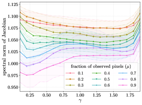
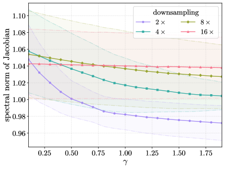
In Fig. 6, we expand our analysis to include a nonlinear trained denoiser [21]. However, since the denoiser is nonlinear, we need to work with the Jacobian of the update operator in (7)––with as the nonlinear denoiser––and its spectral norm. Despite the nonlinearity, we empirically observe in Figs. 4 and 5 that the spectral norms follow a similar pattern. However, since the spectral radius occasionally exceeds 1, the operator cannot be expected to be locally contractive.
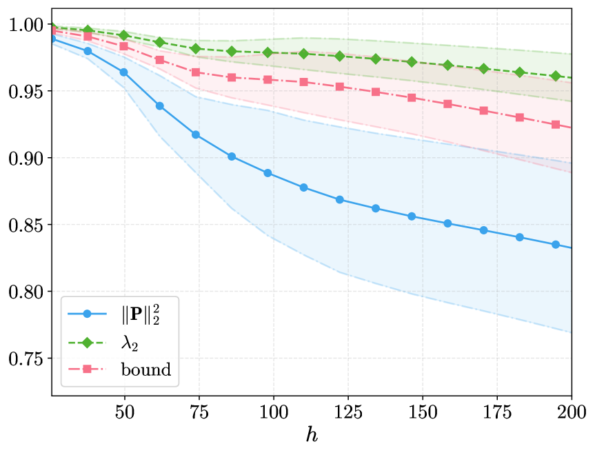
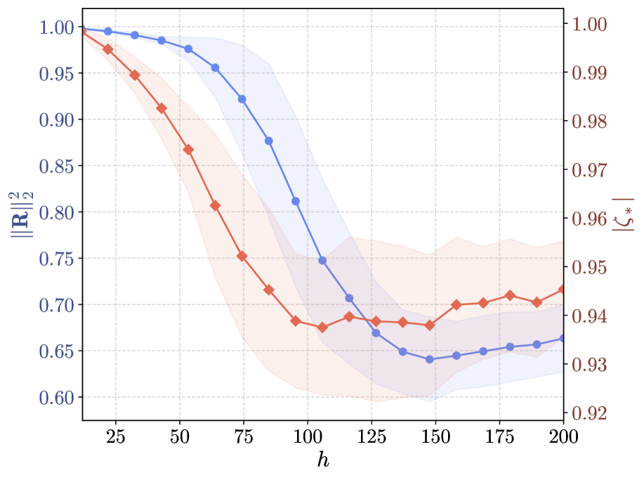
Finally, we study the impact of parameters derived from the denoiser on the convergence. In Fig. 8, we show that a denoiser with a lower results in a smaller contraction factor, consistent with the predictions of Thm. 5. Similarly, Fig. 8 highlights the relation between the contraction factor of PnP-ADMM and , as anticipated in Thm. 6. We decrease (and ) by increasing the bandwidth of the Gaussian kernel. Note that Thms. 5 and 8 do not allow for similar predictions regarding Sc-PnP-ISTA and Sc-PnP-ADMM as the bounds are influenced not only by (or ) but also by . Since both (or ) and are derived from , in the process of changing we also end up altering ––it is not possible to modify one while keeping the other fixed. This contrasts with the symmetric case, which does not exhibit this complex coupling. However, for smaller values of , where changes in have a minimal impact, we observe a reduction in the contraction factor as decreases (see Fig. 9). In Fig. 9, we demonstrate the effects of varying the bandwidth on the convergence of both PnP-ISTA and Sc-PnP-ISTA in practice. Specifically, we observe that while increasing can significantly speed up convergence for both algorithms, an excessive increase in may lead to subpar reconstructions.
VII Conclusion
We proved that the iterates of PnP-ISTA and PnP-ADMM converge globally and linearly to a unique reconstruction when using generic kernel denoisers. This does not follow from standard convex optimization theory since the associated loss function is not strongly convex. The key insight is that the contractivity is not with respect to the standard Euclidean norm but rather a norm induced by the kernel denoiser. This requires modifications to the definition of the gradient in PnP-ISTA and the proximal operator in PnP-ADMM. We also performed experiments with the archetype kernel denoiser, NLM, and its symmetric counterpart, DSG-NLM. We found that the reconstruction quality is typically better for DSG-NLM than NLM. However, DSG-NLM requires about more computations than NLM. Thus, there is a tradeoff between per-iteration cost and reconstruction quality within the class of kernel denoisers.
We derived quantitative bounds on the convergence rate for inpainting, deblurring, and superresolution. The primary challenge was identifying a bound that is . To achieve this, we established various relationships between the parameters of the denoiser and the forward operator. For ADMM, an additional challenge involved evaluating an inverse operator, which we approximated by exploiting specific properties of the forward operator. Nonetheless, there is scope for improving the bounds and using them to optimize the algorithmic parameters.
The derived bounds provide critical insights into the interactions among the different algorithmic components. Notably, we found that the spectral gap of the denoiser significantly influences the convergence rate: the larger the gap, the faster the convergence. However, artificially increasing the spectral gap by adjusting denoiser parameters (such as the bandwidth) is contingent upon the forward operator and may not work in all cases. An interesting question is whether we can design a kernel denoiser with an enhanced spectral gap and deploy it within PnP algorithms to achieve faster convergence without compromising the reconstruction quality.
Acknowledgement
We sincerely thank the editor and the reviewers for their suggestions that helped to improve the paper a lot.
Appendix
VII-A Proof of Lemma 1
VII-B Proof of Lemma 2
Since is self-adjoint, we have
for all , where is an orthonormal basis of eigenvectors of with eigenvalues . In particular, for any ,
Now, using (32), we can write
| (45) |
Furthermore, we can regroup the right side of (45) into
Now, , and by Cauchy-Schwarz. Finally, from , we have . Thus, we obtain
Since this holds for any , we have (33).
VII-C Proof of Thm. 7
References
- [1] Y. Romano, M. Elad, and P. Milanfar, “The little engine that could: Regularization by denoising (RED),” SIAM J. Imaging Sci., vol. 10, no. 4, pp. 1804–1844, 2017.
- [2] S. Sreehari, S. V. Venkatakrishnan, B. Wohlberg, G. T. Buzzard, L. F. Drummy, J. P. Simmons, and C. A. Bouman, “Plug-and-play priors for bright field electron tomography and sparse interpolation,” IEEE Trans. Comput. Imag., vol. 2, no. 4, pp. 408–423, 2016.
- [3] A. Buades, B. Coll, and J.-M. Morel, “Image denoising methods. a new nonlocal principle,” SIAM Review, vol. 52, no. 1, pp. 113–147, 2010.
- [4] K. Dabov, A. Foi, V. Katkovnik, and K. Egiazarian, “Image denoising by sparse 3-D transform-domain collaborative filtering,” IEEE Trans. Image Process., vol. 16, no. 8, pp. 2080–2095, 2007.
- [5] W. Dong, P. Wang, W. Yin, G. Shi, F. Wu, and X. Lu, “Denoising prior driven deep neural network for image restoration,” IEEE Trans. Pattern Anal. Mach. Intell., vol. 41, no. 10, pp. 2305–2318, 2018.
- [6] K. Zhang, Y. Li, W. Zuo, L. Zhang, L. Van Gool, and R. Timofte, “Plug-and-play image restoration with deep denoiser prior,” IEEE Trans. Pattern Anal. Mach. Intell., 2021.
- [7] C. A. Bouman, Foundations of Computational Imaging: A Model-Based Approach. SIAM, 2022.
- [8] K. Zhang, W. Zuo, Y. Chen, D. Meng, and L. Zhang, “Beyond a Gaussian denoiser: Residual learning of deep CNN for image denoising,” IEEE Trans. Image Process., vol. 26, no. 7, pp. 3142–3155, 2017.
- [9] M. Terris, T. Moreau, N. Pustelnik, and J. Tachella, “Equivariant plug-and-play image reconstruction,” Proc. CVPR, pp. 25 255–25 264, 2024.
- [10] P. Nair and K. N. Chaudhury, “Plug-and-play regularization using linear solvers,” IEEE Trans. Image Process., vol. 31, pp. 6344–6355, 2022.
- [11] E. T. Reehorst and P. Schniter, “Regularization by denoising: Clarifications and new interpretations,” IEEE Trans. Comput. Imag., vol. 5, no. 1, pp. 52–67, 2018.
- [12] S. H. Chan, X. Wang, and O. A. Elgendy, “Plug-and-play ADMM for image restoration: Fixed-point convergence and applications,” IEEE Trans. Comput. Imag., vol. 3, no. 1, pp. 84–98, 2017.
- [13] E. Ryu, J. Liu, S. Wang, X. Chen, Z. Wang, and W. Yin, “Plug-and-play methods provably converge with properly trained denoisers,” Proc. Intl. Conf. Mach. Learn., vol. 97, pp. 5546–5557, 2019.
- [14] A. Raj, Y. Li, and Y. Bresler, “GAN-based projector for faster recovery with convergence guarantees in linear inverse problems,” Proc. IEEE Intl. Conf. Comp. Vis., pp. 5602–5611, 2019.
- [15] R. G. Gavaskar and K. N. Chaudhury, “Plug-and-play ISTA converges with kernel denoisers,” IEEE Signal Process. Lett., vol. 27, pp. 610–614, 2020.
- [16] T. Liu, L. Xing, and Z. Sun, “Study on convergence of plug-and-play ISTA with adaptive-kernel denoisers,” IEEE Signal Process. Lett., vol. 28, pp. 1918–1922, 2021.
- [17] R. G. Gavaskar, C. D. Athalye, and K. N. Chaudhury, “On plug-and-play regularization using linear denoisers,” IEEE Trans. Image Process., vol. 30, pp. 4802–4813, 2021.
- [18] R. Cohen, Y. Blau, D. Freedman, and E. Rivlin, “It has potential: Gradient-driven denoisers for convergent solutions to inverse problems,” Proc. Adv. Neural Inf. Process. Syst., vol. 34, 2021.
- [19] R. G. Gavaskar, C. D. Athalye, and K. N. Chaudhury, “On exact and robust recovery for plug-and-play compressed sensing,” Signal Processing, vol. 211, p. 109100, 2023.
- [20] S. Hurault, A. Leclaire, and N. Papadakis, “Gradient step denoiser for convergent plug-and-play,” Proc. ICLR, 2022.
- [21] J.-C. Pesquet, A. Repetti, M. Terris, and Y. Wiaux, “Learning maximally monotone operators for image recovery,” SIAM J. Imaging Sci., vol. 14, no. 3, pp. 1206–1237, 2021.
- [22] R. Cohen, M. Elad, and P. Milanfar, “Regularization by denoising via fixed-point projection (RED-PRO),” SIAM J. Imaging Sci., vol. 14, no. 3, pp. 1374–1406, 2021.
- [23] S. Hurault, A. Leclaire, and N. Papadakis, “Proximal denoiser for convergent plug-and-play optimization with nonconvex regularization,” Proc. ICML, 2022.
- [24] A. Goujon, S. Neumayer, and M. Unser, “Learning weakly convex regularizers for convergent image-reconstruction algorithms,” SIAM J. Imaging Sci., vol. 17, no. 1, pp. 91–115, 2024.
- [25] N. Parikh and S. Boyd, “Proximal algorithms,” Found. Trends. Optim., vol. 1, no. 3, pp. 127–239, 2014.
- [26] A. Beck, First-Order Methods in Optimization. SIAM, 2017.
- [27] J. Eckstein and D. P. Bertsekas, “On the Douglas–Rachford splitting method and the proximal point algorithm for maximal monotone operators,” Mathematical Programming, vol. 55, pp. 293–318, 1992.
- [28] H. Takeda, S. Farsiu, and P. Milanfar, “Kernel regression for image processing and reconstruction,” IEEE Trans. Image Process., vol. 16, no. 2, pp. 349–366, 2007.
- [29] H. Talebi and P. Milanfar, “Global image denoising,” IEEE Trans. Image Process., vol. 23, no. 2, pp. 755–768, 2013.
- [30] P. Nair, V. S. Unni, and K. N. Chaudhury, “Hyperspectral image fusion using fast high-dimensional denoising,” Proc. IEEE Intl. Conf. Image Process., pp. 3123–3127, 2019.
- [31] C. D. Athalye, K. N. Chaudhury, and B. Kumar, “On the contractivity of plug-and-play operators,” IEEE Signal Process. Lett., vol. 30, pp. 1447–1451, 2023.
- [32] C. D. Athalye and K. N. Chaudhury, “Corrections to “On the contractivity of plug-and-play operators”,” IEEE Signal Process. Lett., vol. 30, pp. 1817–1817, 2023.
- [33] K. Zhang, W. Zuo, S. Gu, and L. Zhang, “Learning deep CNN denoiser prior for image restoration,” Proc. IEEE Conf. Comp. Vis. Pattern Recognit., pp. 3929–3938, 2017.
- [34] H. H. Bauschke and P. L. Combettes, Convex Analysis and Monotone Operator Theory in Hilbert Spaces. Springer, 2017.
- [35] P. Nair and K. N. Chaudhury, “Averaged deep denoisers for image regularization,” J. Math. Imaging Vis., pp. 1–18, 2024.
- [36] P. Milanfar, “Symmetrizing smoothing filters,” SIAM J. Imaging Sci., vol. 6, no. 1, pp. 263–284, 2013.
- [37] V. S. Unni, P. Nair, and K. N. Chaudhury, “Plug-and-play registration and fusion,” Proc. IEEE Intl. Conf. Image Process., pp. 2546–2550, 2020.
- [38] Y. Yazaki, Y. Tanaka, and S. H. Chan, “Interpolation and denoising of graph signals using plug-and-play ADMM,” Proc. IEEE Int. Conf. Acoust. Speech Signal Process., pp. 5431–5435, 2019.
- [39] M. Nagahama, K. Yamada, Y. Tanaka, S. H. Chan, and Y. C. Eldar, “Graph signal denoising using nested-structured deep algorithm unrolling,” Proc. IEEE Int. Conf. Acoust. Speech Signal Process., pp. 5280–5284, 2021.
- [40] P. Milanfar, “A tour of modern image filtering: new insights and methods, both practical and theoretical,” IEEE Signal Process. Mag., vol. 30, no. 1, pp. 106–128, 2013.
- [41] C. D. Meyer, Matrix Analysis and Applied Linear Algebra. SIAM, 2000.
- [42] Y. Katznelson, An Introduction to Harmonic Analysis. Cambridge University Press, 2004.
- [43] F. R. Chung, Spectral Graph Theory. AMS, 1997, vol. 92.
- [44] J. J. Moreau, “Proximité et dualité dans un espace Hilbertien,” Bull. Soc. Math. France, vol. 93, pp. 273–299, 1965.
- [45] K. N. Chaudhury, “A concise proof of Moreau’s characterization of proximal operators,” hal-05038838, 2025.
- [46] A. Beck, First-Order Methods in Optimization. SIAM, 2017.
- [47] P. Nair, “Provably Convergent Algorithms for Denoiser-Driven Image Regularization,” PhD thesis, Indian Institute of Science, 2022, available at https://github.com/pravin1390/PhDthesis.
- [48] A. M. Teodoro, J. M. Bioucas-Dias, and M. A. T. Figueiredo, “A convergent image fusion algorithm using scene-adapted Gaussian-mixture-based denoising,” IEEE Trans. Image Process., vol. 28, no. 1, pp. 451–463, 2019.
- [49] R. A. Horn and C. R. Johnson, Matrix Analysis. Cambridge University Press, 1985.