One-Layer Transformers are Provably Optimal for In-context Reasoning and Distributional Association Learning in Next-Token Prediction Tasks

Abstract

We study the approximation capabilities and on-convergence behaviors of one-layer transformers on the noiseless and noisy in-context reasoning of next-token prediction. Existing theoretical results focus on understanding the in-context reasoning behaviors for either the first gradient step or when the number of samples is infinite. Furthermore, no convergence rates nor generalization abilities were known. Our work addresses these gaps by showing that there exists a class of one-layer transformers that are provably Bayes-optimal with both linear and ReLU attention. When being trained with gradient descent, we show via a finite-sample analysis that the expected loss of these transformers converges at linear rate to the Bayes risk. Moreover, we prove that the trained models generalize to unseen samples as well as exhibit learning behaviors that were empirically observed in previous works. Our theoretical findings are further supported by extensive empirical validations.

1 Introduction

Large language models (LLMs) have shown impressive results in complex tasks that require some form of “reasoning” where classical models such as feed-forward networks seem to struggle. These reasoning tasks include, but are not limited to, generating coherent and plausible texts from a given context, language understanding, and mathematical reasoning (Brown et al., 2020; Achiam et al., 2023). At the heart of LLMs is the transformer architecture that features the self-attention mechanism (Vaswani et al., 2017). Transformers can process a long sequence of contexts and enable in-context reasoning via attention mechanisms. Despite such remarkable empirical performance, the theoretical understanding of self-attention in reasoning tasks remains elusive, raising critical risk and safety issues when it comes to the widespread adoption of LLM technology in a socially acceptable manner (Bommasani et al., 2021; Belkin, 2024).

The literature has shown the usefulness of disentangling the behavior of complex models such as LLMs via controlled-setting tasks that we understand the groundtruth behaviors (Allen-Zhu, 2024). For understanding reasoning in LLMs, one of the benchmark tasks that the literature has been recently embarked on is next-token prediction (NTP), wherein the tasks require a model to understand the context from a sentence to be able to predict the next token correcty. As a running example, consider the task of predicting the next token for the sentence “Anna gives a book to” (the same example used in (Chen et al., 2025)). A global bigram statistics would predict the next token to be “the” as the bigram “to the” naturally occurs in English with high frequency. However, if another person appears in the context, say Bob, then “Bob” is perhaps a better token prediction, even though the bigram “to Bob” is not a frequent bigram in the global context. In transformers, there have been strong (both empirically and theoretically) evidence that attention heads seem to responsible for in-context reasoning such as the in-context bigram “to Bob” (Wang et al., 2022) while feedforward layers seem to responsible for storing global statistics or factual knowledge such as the global bigram “to the” (Geva et al., 2020; Meng et al., 2022; Bietti et al., 2023; Nichani et al., 2024).

However, a proper understanding how such capabilities emerge during training is still lacking. For example, it is unclear how distributional associations such as “to the” and in-context reasoning such as “to Bob” are automatically assigned to feed-forward layers and self-attention layers by gradient descent without being explicitly forced to do so during training. Several initial efforts have shed insights into the above question (Chen et al., 2025; Bietti et al., 2023; Nichani et al., 2024). While they made an important first progress, we are still far from depicting the whole picture of how reasoning emerges in transformers. In particular, the existing theoretical results are limited to the reasoning behavior for just the first gradient steps or an infinite-sample setting, which do not reflect how we actually train transformers in practice.

In this paper, we narrow the gap above by providing a more complete picture of training transformers on next-token prediction tasks and how they get assigned with in-context reasoning and distributional association. In particular, we provide a synthetic next-token prediction task that requires a model to differentiate in-context reasoning from distributional association to be able to succeed. We show that one-layer transformers, from either the class of linear or ReLU attentions, suffice to provably approximate the Bayes-optimal predictor of the task. In addition, we show that training these transformers with normalized gradient descents converges at linear rate to the Bayes optimal predictor and exhibit a provable generalization to unseen samples. Furthermore, we show that, after sufficient number of training iterations, feed-forward layer learns to predict the noise token while attention layers learn to predict the true output token, a behavior that has been observed empirically recently. Finally, we corroborate theoretical findings with extensive empirical validations.

1.1 Related Work

Brown et al. (2020) demonstrate that trained transformers can perform in-context learning—adapting to new tasks at inference with only a few examples. Building on this, several studies (Akyürek et al., 2022; Bai et al., 2023; Von Oswald et al., 2023; Giannou et al., 2023) show that appropriately parameterized transformers can simulate procedures like gradient descent. Furthermore, (Yun et al., 2019) prove that transformers can approximate any continuous permutation-equivariant sequence-to-sequence function on compact support.

Several works have analyzed transformers’ training dynamics for in-context learning of linear regression. Ahn et al. (2024) show a one-layer linear transformer that performs a preconditioned gradient step, with $L$ layers corresponding to $L$ steps at certain critical points. Mahankali et al. (2023) find that a one-layer linear transformer trained on noisy data mimics a single least-squares gradient step. Zhang et al. (2024) prove convergence to a global minimum under suitable initialization. Huang et al. (2024a) study gradient descent in softmax transformers learning linear functions. Cui et al. (2024) show that multi-head attention with large embeddings outperforms single-head variants. Cheng et al. (2023) demonstrate that nonlinear transformers can emulate gradient descent on nonlinear functions. Kim and Suzuki (2024) analyze mean-field and two-timescale limits of linear attention models, and Chen and Li (2024) give computational bounds for training multi-head attention layers.

Another line of work investigates the training dynamics for binary classification. Tarzanagh et al. (2023) show that self-attention optimization mirrors hard-margin SVMs, revealing the implicit bias of 1-layer transformers trained via gradient descent, and that over-parameterization aids global convergence. Ataee Tarzanagh et al. (2023) demonstrate that gradient descent on softmax attention converges to a max-margin separator distinguishing locally optimal tokens. Building on this, Vasudeva et al. (2024) provide finite-sample analysis. Deora et al. (2023) offer optimization and generalization guarantees for training single-layer multi-head attention models under the NTK regime.

Recent works have also examined transformers’ training dynamics for next-token prediction (NTP). Tian et al. (2023a) show that self-attention acts as a discriminative scanner, focusing on predictive tokens and down-weighting common ones. Tian et al. (2023b) analyze multilayer dynamics, while Li et al. (2024) find that gradient descent trains attention to learn an automaton via hard retrieval and soft composition. Thrampoulidis (2024) study the implicit bias of gradient descent in linear transformers. Huang et al. (2024b) provide finite-time analysis for a one-layer transformer on a synthetic NTP task, showing sublinear max-margin and linear cross-entropy convergence. Their setting assumes one-to-one token mapping, whereas we address a more general case allowing one-to-many mappings and prove generalization results for this broader task.

Our work also connects to recent views of transformer weight matrices—especially in embedding and feed-forward layers—as associative memories. Bietti et al. (2023) show that transformers store global bigrams and adapt to new context at different rates. Chen et al. (2025) find that feed-forward layers capture distributional associations, while attention supports in-context reasoning, attributing this to gradient noise (though only analyzing one gradient step). Nichani et al. (2024) theoretically analyze gradient flow in linear attention models on factual recall tasks.

2 Problem Setup

Notations. We use bold lowercase letters for vectors and bold uppercase letters for matrices. Let $N$ be the size of the vocabulary, and $\mathcal{V}=[N]:=\{1,\ldots,N\}$ be the vocabulary itself. A token $y\in[N]$ is an element of the vocabulary. A sentence of length $H$ is a sequence of tokens denoted by $z_{1:H}$, where $z_{h}\in[N]$ is the $h$-th element of $z_{1:H}$. We use $C_{x,y}=\sum_{h=1}^{H-1}\mathbb{1}\{z_{h-1}=x,z_{h}=y\}$ to denote the number of times a bigram $(x,y)$ appear in a sentence. Generally, we will use “word” and “token” interchangeably throughout the paper, although we often use “word” to refer to an element of a sentence and “token” to refer to a specific type of elements of the vocabulary.

Definition 2.1.

(Data Model) We study slightly modified variants of the noiseless and noisy in-context reasoning tasks proposed in Bietti et al. (2023) and Chen et al. (2025), respectively. More specifically, we define the following two special, non-overlapping sets of tokens: a set of trigger tokens ${\mathcal{Q}}\subset[N]$ and a set output tokens ${\mathcal{O}}\subset[N]$, where ${\mathcal{O}}\cap{\mathcal{Q}}=\emptyset$. A special “generic” noise token is defined by $\tau=N+1$. The noise level is determined by a constant $\alpha\in[0,1)$, where $\alpha=0$ corresponds to the noiseless learning setting (Bietti et al., 2023) and $\alpha>0$ corresponds to the noisy learning setting (Chen et al., 2025). In our model, a sentence $z_{1:H+1}$ is generated as follows:

• Sample a trigger word $q\sim\mathrm{Unif}({\mathcal{Q}})$ and an output word $y\sim\mathrm{Unif}({\mathcal{O}})$,

• Sample randomly (over an arbitrary distribution) $z_{1:H-1}$ from the set of sentences that satisfy the following three conditions: (I) there exists at least one bigram $(q,y)$ in the sentence, (II) $\tau$ may appear in a sentence only if $\alpha>0$, in that case $\tau$ is always preceded by $q$, and (III) no other (trigger, token) bigrams other than $(q,y)$ or $(q,\tau)$ are in the sentence,

• Fix $z_{H}=q$,

• Set $z_{H+1}=\tau$ with probability $\alpha$ and $z_{H+1}=y$ with probability $1-\alpha$.

Comparisons to existing works. Compared to the existing task modes in Bietti et al. (2023); Chen et al. (2025), our task model offers several notable advantages. First, all sentences in our models must contain at least one (trigger token, output token) bigram, leading to a better signal-to-noise ratio. This allows us to avoid un-informative sentences that contain no useful signals for learning. Second, our task models are agnostic with respect to the distribution of the sentences. In other words, we do not impose any assumptions on how words and sentences are distributed, as long as the conditions are satisfied. Thus, our distributionally agnostic models are both more applicable to practical scenarios and more challenging for theoretical analyses. Third, by restricting the output tokens to a subset of $[N]$, we can study the generalization ability of a model on unseen output tokens. Furthermore, because there are more than one possible next-token for every trigger word, our next-token prediction task is more challenging than the task of learning a one-to-one token mapping in Huang et al. (2024b).

One-layer Decoder-only Transformers. To establish the theoretical guarantees of the optimality and on-convergence behaviors of transformers, we adopt the popular approach in existing works (Bietti et al., 2023; Chen et al., 2025; Huang et al., 2024a, e.g.) and consider the following one-layer transformer model, which is a variant of the model in Chen et al. (2025). Let $E:[N]\mapsto\mathbb{R}^{d}$ be the input word embedding, i.e. $E(z)\in\mathbb{R}^{d}$ is the input embedding of the word $z\in[N]$, and $\tilde{E}:[N]\mapsto\mathbb{R}^{d}$ be a (different) embedding representing the previous token head construction as in Bietti et al. (2023). Let ${\bm{U}}\in\mathbb{R}^{N\times d},{\bm{V}}\in\mathbb{R}^{d\times d},{\bm{W}}\in\mathbb{R}^{d\times d}$ be the unembedding matrix, the value matrix and the joint query-key matrix, respectively. Our model consists of one attention layer and one feed-forward layer. The input ${\mathbf{x}}_{1:H}$ and the output of the model are as below.

$${\mathbf{x}}_{h} =E(z_{h})+\tilde{E}(z_{h-1})\in\mathbb{R}^{d},$$ (1)

$$\phi({\bm{x}}_{H},{\bm{x}}_{1:H}) ={\bm{V}}\sum_{h=1}^{H}\sigma({\bm{x}}_{H}^{\top}{\bm{W}}{\bm{x}}_{h}){\bm{x}}_{h}\in\mathbb{R}^{d},$$

$$\xi_{A} ={\bm{U}}\phi({\bm{x}}_{H},{\bm{x}}_{1:H})\in\mathbb{R}^{N},$$

$$\xi_{F} ={\bm{U}}{\bm{F}}\left({\bm{x}}_{H}+\sum_{h=1}^{H}\sigma(x_{H}^{\top}{\bm{W}}{\bm{x}}_{h}){\bm{x}}_{h}\right),$$

where ${\bm{F}}$ is the matrix of the linear layer and $\sigma:\mathbb{R}\to\mathbb{R}$ is the activation function which determines the range of the attention scores. For theoretical analyses, we use linear attention $\sigma({\bm{x}}_{H}^{\top}{\bm{W}}{\bm{x}}_{h})={\bm{x}}_{H}^{\top}{\bm{W}}{\bm{x}}_{h}$ and ReLU attention $\sigma({\bm{x}}_{H}^{\top}{\bm{W}}{\bm{x}}_{h})=\max(0,{\bm{x}}_{H}^{\top}{\bm{W}}{\bm{x}}_{h})$. For empirical analyses, we additionally use softmax attention $\sigma({\bm{x}}_{H}^{\top}{\bm{W}}{\bm{x}}_{h})=\frac{\exp({\bm{x}}_{H}^{\top}{\bm{W}}{\bm{x}}_{h})}{\sum_{j=1}^{H}\exp({\bm{x}}_{H}^{\top}{\bm{W}}{\bm{x}}_{j})}$. The final logit is $\xi=\xi_{A}+\xi_{F}$.

Compared to Chen et al. (2025), our model in (1) differs in the computation of $\xi_{F}$. More specifically, while their theoretical model used $\xi_{F}={\bm{U}}{\bm{F}}{\bm{x}}_{H}$, we add the input $\sum_{h=1}^{H}\sigma(x_{H}^{\top}{\bm{W}}{\bm{x}}_{h}){\bm{x}}_{h}$ to the feed-forward layer, which is more similar to the empirical model that was used for the experiments in Chen et al. (2025). As we will show in Section 4, this modification is sufficient for showing the Bayes-optimality of one-layer transformers. Next, similar to Chen et al. (2025), we fix the embedding maps $E,\tilde{E},{\bm{U}}$ and use cross-entropy loss on $\xi$, i.e. the population loss is

$$L =\mathbb{E}_{q,y,{\bm{z}}}\left[-\ln\frac{\exp(\xi_{y})}{\sum_{j\in[N]}\exp(\xi_{j})}\right].$$ (2)

To facilitate the analysis, we employ the following commonly used assumption, which is also the first part of Assumption F.1 in Chen et al. (2025).

Assumption 2.2.

(Orthonormal Embedding) For any $i,j\in[N]$, we have $E(i)^{\top}E(j)=\tilde{E}(i)^{\top}\tilde{E}(j)=\mathbb{1}\{i=j\}$ and $E(i)^{\top}\tilde{E}(j)=0$.

Remark 2.3.

Assumption 2.2 necessarily implies that $d\geq N$. This condition is not too strict as transformers may need sufficient memory capability to remember the vocabulary before they can perform any meaningful in-context reasoning. This is consistent with suggestions in recent literature on the memorization capacity of transformers, where the embedding dimension or the number of heads is polynomially larger than the vocabulary size (Nichani et al., 2024; Mahdavi et al., 2023; Madden et al., 2024).

3 Noiseless Learning ($\alpha=0$)

In this section, we consider the noiseless learning setting in which $\alpha=0$ and $\tau$ never appears in a sentence. In Section˜3.1, we prove the approximation capability of the model defined in (1) by showing that there exists a reparameterization of ${\bm{U}},{\bm{V}},{\bm{F}}$ and ${\bm{W}}$ that drives the population loss (2) to $0$. In Section˜3.2, we show that the reparameterized model can be trained by normalized gradient descent and the population loss converges to $0$ at linear rate.

3.1 Approximation Capabilities of One-Layer Transformers On Noiseless Setting

We show that for any instance of the noiseless data model in Definition 2.1, there is a one-layer transformer that precisely approximates the task instance, i.e., the population loss is zero. To this end, we initialize and freeze the matrix ${\bm{F}}=\mathbf{0}$ so that $\xi_{F}=\mathbf{0}$. The population loss becomes

$$L({\bm{V}},\!\!{\bm{W}}) \!=\!\mathbb{E}_{q,y,{\bm{z}}}\!\left[\!-\ln\frac{e^{\xi_{A,y}}}{\sum_{j\in[N]}e^{\xi_{A,j}}}\right]\!\!=\!\!\mathbb{E}_{q,y,{\bm{z}}}\!\!\left[\!-\ln\frac{e^{{\bm{e}}_{y}^{\top}{\bm{U}}{\bm{V}}\sum_{h=1}^{H}\sigma({\bm{x}}_{H}^{\top}{\bm{W}}{\bm{x}}_{h}){\bm{x}}_{h}}}{\sum_{j\in[N]}e^{{\bm{e}}_{j}^{\top}{\bm{U}}{\bm{V}}\sum_{h=1}^{H}\sigma({\bm{x}}_{H}^{\top}{\bm{W}}{\bm{x}}_{h}){\bm{x}}_{h}}}\right],$$ (3)

where ${\bm{e}}_{j}$ is the $j$-th vector in the canonical basis of $\mathbb{R}^{N}$ (i.e., $[{\bm{e}}_{j}]_{k}=\mathbb{1}\{j=k\}$). Note that the output embedding ${\bm{U}}$ is considered a fixed matrix as in Chen et al. (2025), thus the population loss is a function of ${\bm{V}}$ and ${\bm{W}}$. We consider a specific parametric class of the weight matrices ${\bm{U}},{\bm{V}}$ and ${\bm{W}}$. In particular, the following lemma shows that there exists a reparameterization of ${\bm{U}},{\bm{V}}$ and ${\bm{W}}$ that makes the population loss arbitrarily close to $0$. The proof is in Appendix A.1.

Lemma 3.1.

Let $\bm{\lambda}=\{\lambda_{k}\in\mathbb{R}_{+}:k\in{\mathcal{Q}}\}$ be a set of $\absolutevalue{{\mathcal{Q}}}$ of non-negative values. Under Assumption 2.2, by setting ${\bm{U}}=[E(1)~E(2)~\dots~E(N)]^{\top},{\bm{V}}={\bm{I}}_{d}$ and ${\bm{W}}=\sum_{k\in{\mathcal{Q}}}\lambda_{k}E(k)\tilde{E}^{\top}(k)$, for both linear and ReLU attention, we obtain

$$\lim_{\bm{\lambda}\to\infty}L(\bm{\lambda})\vcentcolon=\lim_{(\lambda_{q})_{q\in{\mathcal{Q}}}\to\infty}L\left({\bm{I}}_{d},\sum_{q\in{\mathcal{Q}}}\lambda_{q}E(q)\tilde{E}^{\top}(q)\right)=0.$$ (4)

Proof.

(Sketch) For linear and ReLU attention, it can be shown that the attention score of the $h$-th token $z_{h}$ is $\sigma({\bm{x}}_{H}^{\top}{\bm{W}}{\bm{x}}_{h})=\mathbb{1}\{z_{h-1}=q\}$. In other words, the attention scores ${\bm{x}}_{H}^{\top}{\bm{W}}{\bm{x}}_{h}$ is a non-zero (and positive) value for $x_{h}$ only when $z_{h-1}$ is the trigger word. As a result, the logits of token $j\in[N]$ is $\xi_{j}=\xi_{A,j}=\lambda_{q}C_{q,y}\mathbb{1}\{j=y\}$. It follows that the probability of outputting $y$ is $\lim_{\lambda_{q}\to\infty}\frac{\exp(\xi_{y})}{\sum_{j\in[N]}\exp(\xi_{j})}=\lim_{\lambda_{q}\to\infty}\frac{\exp(C_{q,y}\lambda_{q})}{\exp(C_{q,y}\lambda_{q})+N-1}=1$. ∎

3.2 Training Dynamics and On-Convergence Behavior: A Distributionally Agnostic Analysis

We analyze the gradient descent training dynamics in training one-layer linear transformers parameterized in Section˜3.1. Directly running gradient descent on (3) w.r.t $({\bm{V}},{\bm{W}})$ is difficult due to the fact that the cross-entropy loss may not be jointly-convex with respect to $({\bm{V}},{\bm{W}})$. Previous works (e.g. Ahn et al., 2024; von Oswald et al., 2024) have shown that theoretical insights from the optimization dynamics in linearized transformers generalize well to empirical results of non-linear attentions. Inspired by these works, we focus on characterizing the training dynamics, on-convergence behavior and generalization capability of our model using linear attention. In the following, we show that with linear attention, the population loss converges linearly to zero and the trained model generalizes to unseen output tokens.

Convergence rate of normalized gradient descent. From the proof sketch of Lemma 3.1, the population loss $L(\bm{\lambda})$ is $L(\bm{\lambda})=\mathbb{E}_{q,y,z}\left[-\ln\frac{\exp(C_{q,y}\lambda_{q})}{\exp(C_{q,y}\lambda_{q})+N-1}\right]$. We initialize $\bm{\lambda}_{0}=\mathbf{0}$. Running standard gradient descent $\bm{\lambda}_{t+1}=\bm{\lambda}_{t}-\eta\nabla_{\bm{\lambda}}L$, where $\eta>0$ is the learning rate, would require knowing the exact distribution of $z$ since $C_{q,y}$ is a random variable depending on $z$. Instead, we adopt a normalized gradient descent algorithm, where

$$\bm{\lambda}_{t+1}=\bm{\lambda}_{t}-\eta\frac{\nabla_{\bm{\lambda}}L}{\norm{\nabla_{\bm{\lambda}}L}_{2}},$$ (5)

i.e. the gradient vectors are normalized by their Euclidean norm. A similar normalized gradient descent update for transformers has been used in Huang et al. (2024b) for learning an injective map on the vocabulary $[N]$. The following theorem shows that the update rule (5) can be implemented without the knowledge of the distribution of $z$. Moreover, the population loss converges at a linear rate to zero. The proof can be found in Appendix A.2.

Theorem 3.2.

Starting from $\lambda_{q,0}=0$ for all $q\in{\mathcal{Q}}$, the update rule (5) is equivalent to $\lambda_{q,t}=\frac{\eta t}{\absolutevalue{{\mathcal{Q}}}}$ for all $t\geq 1$. Moreover, $L(\bm{\lambda}_{t})=O(N\exp(-t))$.

Generalization to unseen output words. The only correct strategy for solving the noiseless data model in Definition 2.1 is to predict the word that comes after a trigger token. That is, the position of the trigger token is the only important factor in this task. Such a strategy would easily generalize to a sentence which contains a new bigram $(q,y_{\mathrm{test}})$, where $y_{\mathrm{test}}$ is a non-trigger non-output word. We characterize this generalization ability of our parameterized transformers in the following theorem.

Theorem 3.3.

Fix any $y_{\mathrm{test}}\in[N]\setminus({\mathcal{O}}\cup{\mathcal{Q}})$. Take any test sentence generated by the noiseless data model, except that every bigram $(b,y)$ is replaced with $(q,y_{\mathrm{test}})$. Then, our model after being trained by normalized gradient descent for $t$ steps, predicts $y_{\mathrm{test}}$ with probability

$$\Pr[z_{H+1}=y_{\mathrm{test}}\mid\bm{\lambda}_{t}]\vcentcolon=\frac{\exp(\xi_{y_{\mathrm{test}}})}{\sum_{j\in[N]}\exp(\xi_{j})}\geq\frac{\exp(\eta t)}{\exp(\eta t)+N-1}.$$

In particular, this implies that $\Pr[z_{H+1}=y_{\mathrm{test}}\mid\bm{\lambda}_{t}]\geq 0.5$ for $t\geq\ln(N)/\eta$.

Reparameterization versus Directional Convergence. In addition to the convergence of the loss function, existing works (e.g. Ji and Telgarsky, 2021; Huang et al., 2024b) on the training dynamics of neural networks learned with cross-entropy loss have shown that the trainable matrices directionally convergence to an optimal solution. More formally, a sequence of ${\bm{A}}_{t}$ directionally converges to some ${\bm{A}}_{*}$ if $\lim_{t\to\infty}\langle\frac{{\bm{A}}_{t}}{\norm{{\bm{A}}_{t}}},\frac{{\bm{A}}_{*}}{\norm{{\bm{A}}_{*}}}\rangle=1$.

In our work, the joint query-key matrix ${\bm{W}}$ is reparameterized as a form of associative memory of the trigger tokens, rather than emerging from runing gradient descent for minimizing the population loss $L$, as in  (Bietti et al., 2023; Chen et al., 2025) This raises a natural question: if we use the reparameterization on ${\bm{U}}$ and ${\bm{V}}$ but not ${\bm{W}}$, will running gradient descent on ${\bm{W}}$ directionally converges to $\sum_{q}E(q)\tilde{E}^{\top}(q)$? Theorem 3.4 (full proof in Appendix A.4) provides a negative answer.

Theorem 3.4.

Under ˜2.2, for any $N\geq 4$, there exists an instance of ${\mathcal{O}},{\mathcal{Q}}$ and sentence distribution in the noiseless setting such that with ${\mathcal{Q}}=\{q\},\absolutevalue{{\mathcal{O}}}=2$, ${\bm{W}}^{*}\vcentcolon=E(q)\tilde{E}^{\top}(q)$, ${\bm{U}}$ and ${\bm{V}}$ defined in Lemma 3.1, running standard gradient descent on ${\bm{W}}$ from initialization ${\bm{W}}_{0}=\mathbf{0}$ satisfies

$$\lim_{t\to\infty}\absolutevalue{\langle\frac{{\bm{W}}_{t}}{\norm{{\bm{W}}_{t}}},\frac{{\bm{W}}^{*}}{\norm{{\bm{W}}^{*}}}\rangle}=\frac{2}{\sqrt{12}}<1.$$

Remark 3.5.

Theorem 3.4 can be easily extended to a high-probability statement if ${\bm{W}}_{0}$ is randomly initialized from a Gaussian distribution. This result shows that the space of optimal solutions for this in-context reasoning problem is much more complicated than that of the max-margin problems trained with logistic loss in Ji and Telgarsky (2021); Huang et al. (2024b). Moreover, directional convergence cannot fully characterize the set of optimal solutions.

4 Noisy Learning ($\alpha>0$)

Recall that our noisy data model is a variant of the setting in Chen et al. (2025). Similar to Chen et al. (2025), we assume that there is only one trigger token $q$, i.e. ${\mathcal{Q}}=\{q\}$. Unlike Chen et al. (2025), we allow any distributions of bigrams $(q,y)$ and $(q,\tau)$ in the sentence, and do not assume that the ratio of the frequencies of the bigrams $(q,\tau)$ and $(q,y)$ is $\frac{\alpha}{1-\alpha}$. In other words, our results are based on the distribution of the label $z_{H+1}$ instead of the distribution of the bigrams $(q,\tau)$ and $(q,y)$. We emphasize that a Bayes-optimal solution for our noisy data model will also be a Bayes-optimal solution for the model in Chen et al. (2025).

4.1 Approximation Capabilities of One-Layer Transformers On Noisy Setting

First, we show that by relying on just the distribution of $z_{H+1}$, our one-layer transformer in (1) is capable of making the population loss arbitrarily close to the loss of the Bayes optimal strategy. We start by characterizing the Bayes optimal strategy. Fix an output word $y$. The label of a sentence that contains both $(q,\tau)$ and $(q,y)$ is either $\tau$ with probability $\alpha$ or $y$ with probability $1-\alpha$, independent of other tokens in the sentence. Thus, the Bayes optimal strategy is to predict $\tau$ and $y$ with the same probabilities. Let $\hat{y}$ be the prediction of this strategy. Its expected loss is equal to the entropy

$$L_{\mathrm{Bayes}} =\Pr(z_{H+1}=\tau)(-\ln(\Pr_{\mathrm{Bayes}}(\hat{y}=\tau))+\sum_{y\in{\mathcal{O}}}\Pr(z_{H+1}=y)(-\ln(\Pr_{\mathrm{Bayes}}(\hat{y}=y))$$

$$=-\alpha\ln\alpha-(1-\alpha)\ln(1-\alpha).$$

The following lemma shows that using linear and ReLU attentions, applying softmax on $\xi=\xi_{A}+\xi_{F}$ leads to a Bayes optimal strategy as $\lambda\to\infty$.

Lemma 4.1.

Let $y\in{\mathcal{O}}$ be arbitrary and $\lambda,\gamma\in\mathbb{R}$. Under Assumption 2.2, by setting ${\bm{U}}=[E(1)~E(2)~\dots~E(N)~E(N+1)]^{\top},{\bm{V}}={\bm{I}}_{d},{\bm{W}}=\lambda(E(q)\tilde{E}^{\top}(q)-E(q)E^{\top}(\tau))$ and ${\bm{F}}=E(\tau)(\gamma E^{\top}(q)+\tilde{E}^{\top}(q))$, for all $\alpha\in(0,1)$, for both linear and ReLU attention, we obtain

$$\lim_{\lambda\to\infty,\gamma\to\ln\frac{\alpha}{1-\alpha}}L(\lambda,\gamma)\vcentcolon=\lim_{\lambda\to\infty,\gamma\to\ln\frac{\alpha}{1-\alpha}}\mathbb{E}_{y,z_{1:H+1}}\left[-\ln\frac{\exp(\xi_{z_{H+1}})}{\sum_{j\in[N+1]}\exp(\xi_{j})}\right]=L_{\mathrm{Bayes}}.$$ (6)

Remark 4.2.

Lemma 4.1 is distribution-agnostic in the sense that it holds for any word distribution as long as the three conditions of the data model are satisfied. Moreover, our result holds even for $\alpha>0.5$. This is a major advantage over the existing results in Chen et al. (2025), which required $\alpha\leq 0.5$. Setting $\alpha>0.5$ also reflects a wider range of practical scenarios where the generic bigrams such as “of the” often appear more frequently than context-dependent bigrams such as “of Bob”.

4.2 Training Dynamics and On-Convergence Behavior: A Finite-Sample Analysis

Similar to Section 3.2, we focus on the analysis of linear attention. Let $M$ denote the size of a dataset of $M$ i.i.d sentences $z_{H+1}$ generated from the data model in Definition 2.1. Instead of minimizing the full population loss as in existing works (Bietti et al., 2023; Huang et al., 2024a; Chen et al., 2025), which would require either knowing $\alpha$ or taking $M\to\infty$, we aim to derive a finite-sample analysis that holds for finite $M$ and unknown $\alpha$.

Before presenting our training algorithm and its finite-sample analysis, we first discuss the easier case where $\alpha$ is known and explain why it is difficult to derive the convergence rate of the population loss in (20). Observe that the function $f_{C}(\lambda,\gamma)=-C\lambda-\alpha\gamma+\ln(e^{C\lambda}+e^{C\lambda+\gamma}+N-1)$ is jointly convex and 1/2-smooth with respect to $\lambda$ and $\gamma$. Hence, at first glance, it seems that the convergence rate of $L(\lambda,\gamma)=\mathbb{E}_{C}[f_{C}(\lambda,\gamma)]$ follows from existing results in (stochastic) convex and smooth optimization (Nemirovski et al., 2009). However, as a convex function on unbounded domain with negative partial derivatives, no finite minimizer exists for $L(\lambda,\gamma)$. This implies that minimizing $L(\lambda,\gamma)$ is a multi-dimensional convex optimization problem on astral space (Dud´ık et al., 2022). To our knowledge, nothing is known about the convergence rate to the infimum for this problem.

Training Algorithm. Our approach for solving this astral space issue is to estimate $\gamma$ directly from the dataset and then run normalized gradient descent on $\lambda$. More specifically, recall that $M$ is the number of i.i.d. sentences $z^{(m)}_{1:H+1}$ in the training set. We use the superscript ${(m)}$ to denote quantities that belong to the $m$-th sentence, where $m\in[M]$. Let $M_{\tau}=\sum_{m=1}^{M}\mathbb{1}\{z_{H+1}^{(m)}=\tau\}$ be the number of sentences where $z_{H+1}$ is $\tau$. Let $\hat{\alpha}=\frac{M_{\tau}}{M}$ and $\hat{\gamma}=\ln\frac{\hat{\alpha}}{1-\hat{\alpha}}$ be the unbiased estimates for $\alpha$ and $\gamma=\frac{\ln{\alpha}}{1-\alpha}$, respectively. To avoid notational overload, we write $C^{(m)}_{q,y}$ for $C^{(m)}_{q,y^{(m)}}$. We use $\hat{\gamma}$ in the parameterization of ${\bm{F}}$, i.e. ${\bm{F}}=E(\tau)(\hat{\gamma}E^{\top}(q)+\tilde{E}^{\top}(q))$, and then use this ${\bm{F}}$ to compute the logits $\xi^{(m)}$ for the $m$-th sentence. The empirical loss is

$$L_{\mathrm{emp}}(\lambda) =\frac{1}{M}\sum_{m=1}^{M}-\ln\frac{\exp(\xi_{z_{H+1}}^{(m)})}{\sum_{j\in[N+1]}\exp(\xi_{j}^{(m)})}.$$ (7)

Then, we run normalized gradient descent on $L_{\mathrm{emp}}(\lambda)$ with a constant learning rate $\eta>0$. The formal procedure is given in Algorithm 1 in Appendix B.2. The convergence of the population loss of this algorithm is stated in the following theorem.

Theorem 4.3.

With probability at least $1-\delta$ over the training set of size $M$, after $t$ iterations of normalized gradient descent on (7), Algorithm 1 guarantees that

$$L(\lambda_{t},\hat{\gamma})\leq L_{\mathrm{Bayes}}+\frac{1}{\min(\alpha,1-\alpha)-\sqrt{\frac{\ln(2/\delta)}{2M}}}\frac{\ln(2/\delta)}{2M}+(N-1)e^{-\eta t}.$$

Generalization to unseen output words. Theorem 4.3 indicates that the population loss converges to the Bayes-risk as $M$ and $t$ increases. Next, the following theorem shows that Algorithm 1 produces a trained model that generalizes to an unseen output word $\hat{y}\notin{\mathcal{O}},\hat{y}\neq q$. The proof is in Appendix B.3.

Theorem 4.4.

Fix any $y_{\mathrm{test}}\in[N]\setminus({\mathcal{O}}\cup{\mathcal{Q}})$. Take any test sentence generated by the noisy data model, except that every bigram $(b,y)$ is replaced with $(q,y_{\mathrm{test}})$. Then, with probability at least $1-\delta$, after $t$ iterations, Algorithm 1 returns a model that predicts $y_{\mathrm{test}}$ and $\tau$ with probabilities

$$\Pr[z_{H+1}=\hat{y}\mid\lambda_{t},\hat{\gamma}] \vcentcolon=\frac{\exp(\xi_{y_{\mathrm{test}}})}{\sum_{j\in[N+1]}\exp(\xi_{j})}=1-\alpha+O\left(\sqrt{\frac{\ln(1/\delta)}{M}}+N^{2}e^{-2\eta t}\right),$$

$$\Pr[z_{H+1}=\tau\mid\lambda_{t},\hat{\gamma}] \vcentcolon=\frac{\exp(\xi_{\tau})}{\sum_{j\in[N+1]}\exp(\xi_{j})}=\alpha+O\left(\sqrt{\frac{\ln(1/\delta)}{M}}+N^{2}e^{-2\eta t}\right).$$

Feed-forward layer learns to predict noise while attention layer learns to predict output tokens. An important empirical on-convergence behavior observed in Chen et al. (2025) is that after training, given a sentence which contains both bigrams $(q,y)$ and $(q,\tau)$, the feed-forward layer tends to predict the noise token $\tau$ while the attention layer tends to predict the output token $y$. This property can be expressed formally in terms the final logits as

$$\xi_{A,y}>\max_{j\neq y}\xi_{A,j}\text{ and }\max_{j\neq\tau}\xi_{F,j}<\xi_{F,\tau}.$$ (8)

The following theorem shows that after a sufficiently large number of iterations, Algorithm 1 returns a model that satisfies condition (8) for any input sentence generated from our data model.

Theorem 4.5.

Algorithm 1 guarantees that with probability at least $1-\delta$, after $t\geq\max(1,\frac{1}{\eta}\absolutevalue{\ln(1-\alpha+\sqrt{\frac{\ln(2/\delta)}{2M}})-\ln(\alpha-\sqrt{\frac{\ln(2/\delta)}{2M}})}$ iterations, the condition (8) holds for any sentence generated from the noisy data model.

5 Empirical Validation

Methods	Full input to $\xi_{F}$?	Noiseless		Noisy
		$0$-Loss?	Unseen $y$?	Bayes-Loss?	Unseen $y$?
Origin-Softmax-F	—	—	—	—	—
Origin-Softmax-FA	✓	✓	—	✓	—
Origin-Linear-F	—	—	—	—	—
Origin-Linear-FA	✓	✓	—	✓	—
Origin-ReLU-F	—	✓	—	✓	—
Origin-ReLU-FA	✓	✓	—	✓	—
Reparam-Softmax-F	—	—	✓	—	✓
Reparam-Softmax-FA	✓	—	✓	—	✓
Reparam-Linear-F	—	✓	✓	—	✓
lightgray Reparam-Linear-FA	✓	✓	✓	✓	✓
Reparam-Linear-W-FA	✓	✓	—	✓	—
Reparam-ReLU-F	—	✓	✓	—	✓
lightgray Reparam-ReLU-FA	✓	✓	✓	✓	✓

Table 1: Performance comparison of original (no reparameterization) and parameterized models when being trained on the population loss. 0-Loss and Bayes-loss indicate whether a model’s population loss converges to $0$ or the Bayes risk on noiseless and noisy settings, respectively. Unseen $y$ indicate whether the performance of a model generalizes to unseen output words. Highlighted methods are both Bayes-optimal and generalize to unseen output words.

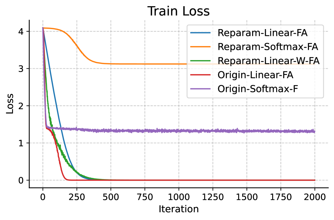
(a)

(b)

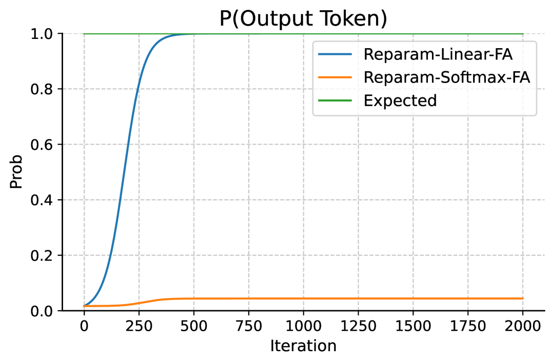
(c)

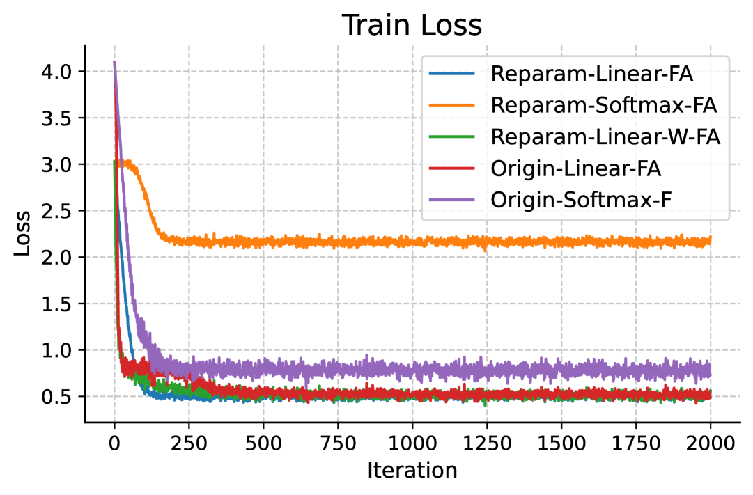
(d)

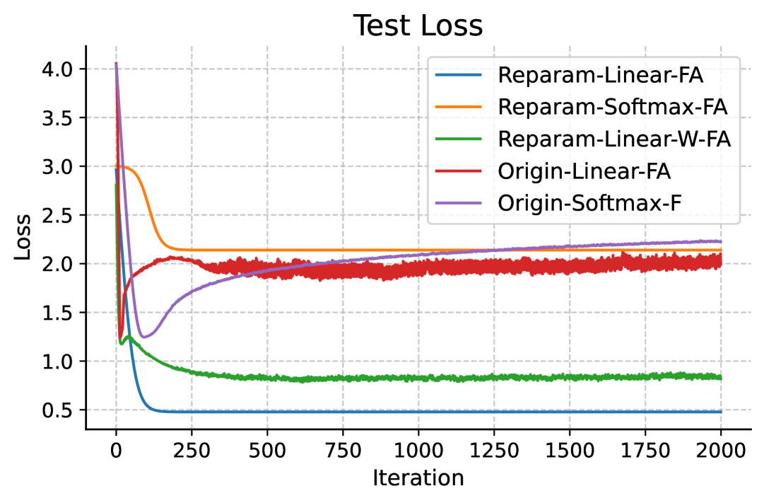
(e)

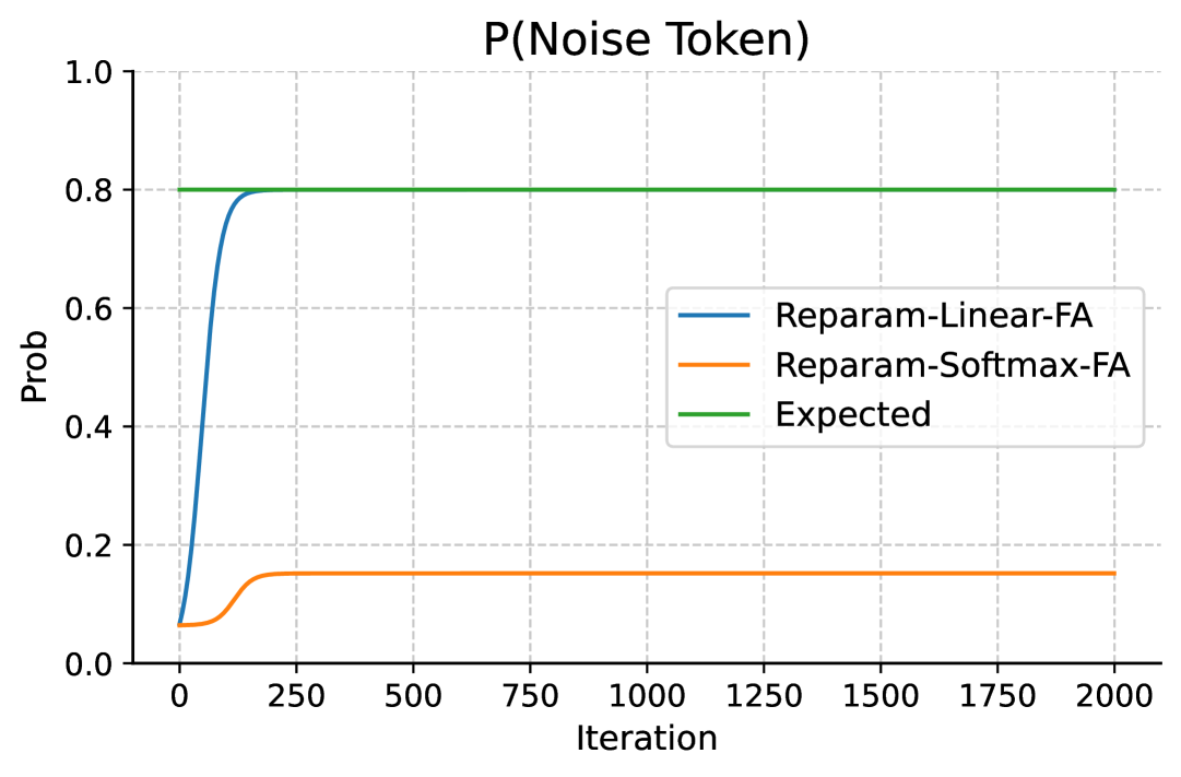
(f)

Figure 1: Models’ performance when being trained on the population loss for $2000$ iterations. First row, left to right: the population loss, unseen output words test loss and the probability of predicting the output tokens in noiseless learning. Second row, left to right: population loss, unseen output words test loss and the probability of predicting the the noise token in noisy learning with $\alpha=0.8$.

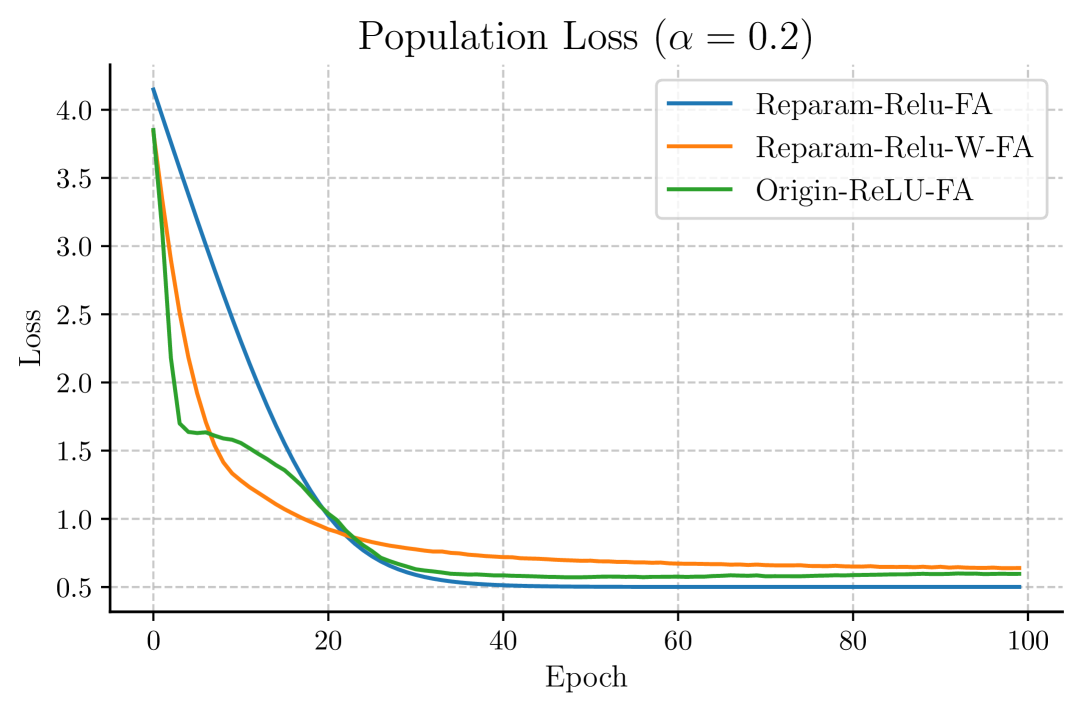
(a)

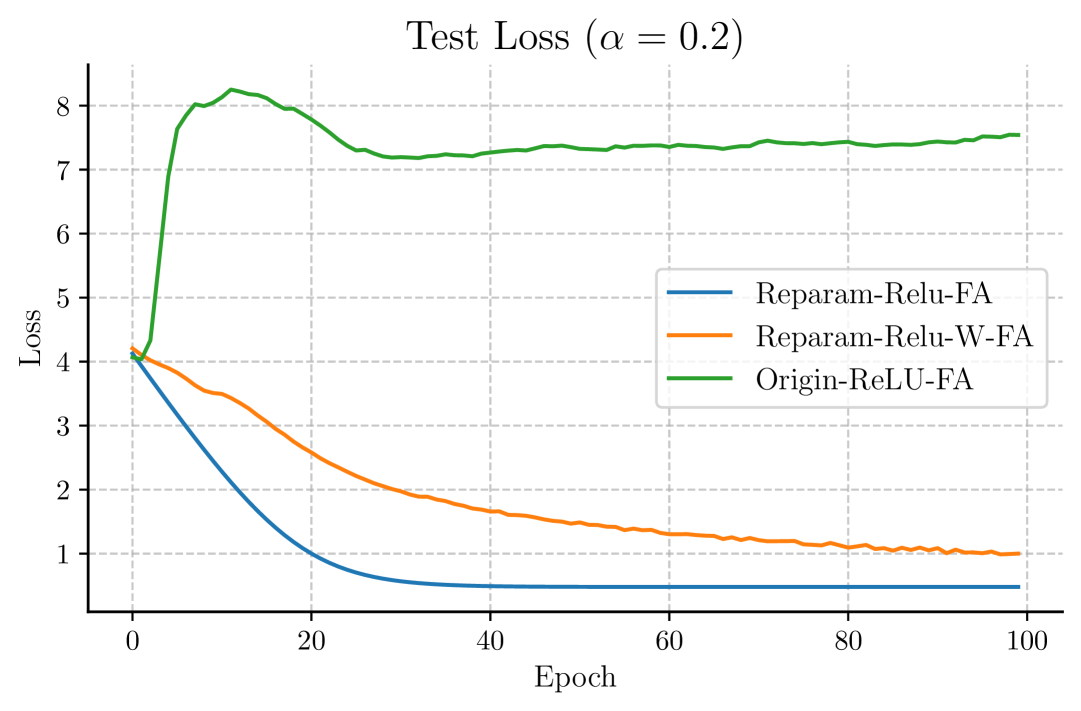
(b)

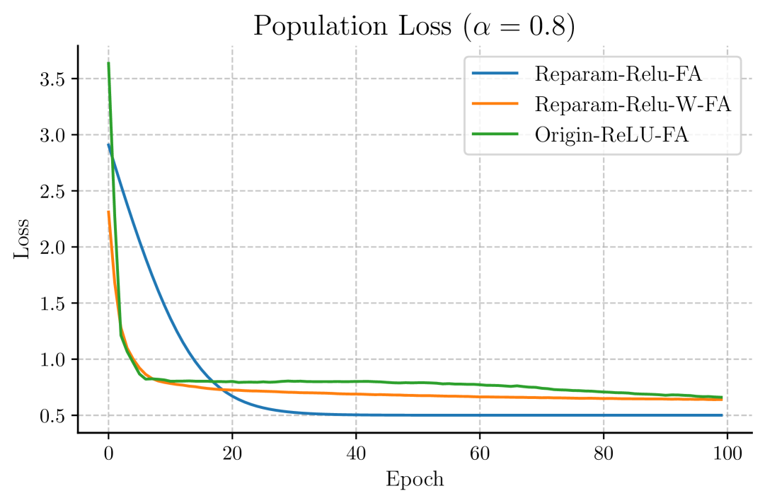
(c)

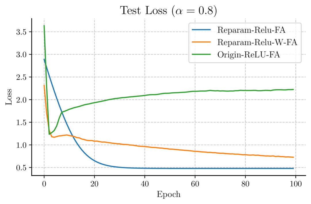
(d)

Figure 2: Three models’ population loss and unseen output words test loss when being trained for $100$ epochs on a dataset of $M=2048$ i.i.d sentences, drawn from the noisy data model with $\alpha\in\{0.2,0.8\}$.

To understand the impacts on empirical performances of the reparameterization presented in Sections 3 and 4, we evaluate the one-layer transformers (1) with different choices of parameterization and attention activation functions on the following data model.

Data Model’s Parameters. We set the vocabulary size $N=60$, the embedding dimension $d=128$ and the context length $H=256$. We use $Q=5$ trigger words and $O=4$ output words. The orthogonal embeddings are the standard basis vectors in $\mathbb{R}^{d}$. Note that the unembedding matrix ${\bm{U}}$ is fixed to be the transpose of the embedding matrix in all of our experiments. For the noisy setting, we choose $\alpha\in\{0.2,0.5,0.8\}$. Our setup generally matches existing works Bietti et al. (2023); Chen et al. (2025).

Our sentences are generated by picking uniformly at random a position for the bigram $(q,y)$ and a position for the bigram $(q,\tau)$ (if the noisy setting). All other words in a sentence are chosen uniformly at random from the set $[N]\setminus({\mathcal{Q}}\cup{\mathcal{O}})$. Whenever the population loss is minimized, we run normalized gradient descent with batch size $512$ over $T=2000$ steps. For the finite-sample analysis, we train the models for $100$ epochs on a fixed training set of $M=2048$ samples. The learning rates are in the range $[0.01,0.5]$. Further details and results can be found in Appendix D.

Baselines. We compare $13$ different models which differ in one or more following aspects: model type (Reparam versus Origin), attention type (linear versus ReLU versus Softmax), input to the feed-forward layer (F versus FA) and whether the joint query-key matrix ${\bm{W}}$ is trained in full without reparameterization. More specifically, the term Origin refers to a model where the three trainable matrices ${\bm{V}},{\bm{W}}$ and ${\bm{F}}$ are trained without reparameterization, while Param indicates that they are re-parameterized as in Lemmas 3.1 and 4.1. We use FA to denote that the feed-forward layer takes the attention-weighted sum $\sum_{h=1}^{H}\sigma(x_{H}^{\top}{\bm{W}}{\bm{x}}_{h}){\bm{x}}_{h}$ as an input, i.e., $\xi_{F}={\bm{U}}{\bm{F}}({\bm{x}}_{H}+\sum_{h=1}^{H}\sigma(x_{H}^{\top}{\bm{W}}{\bm{x}}_{h}){\bm{x}}_{h})$, and F to denote the opposite. Note that Origin-Softmax-F corresponds to the one-layer transformer in Chen et al. (2025). Finally, the model whose name contains both Reparam and -W has ${\bm{V}}$ and ${\bm{F}}$ re-parameterized but ${\bm{W}}$ is trained in full (as in Theorem 3.4).

5.1 Population Loss Convergence

We train $13$ models, shown in Table 1, to minimize the population loss of noiseless and noisy settings. In the noiseless setting, four models fail to minimize the population loss to $0$. Two of these models are re-parameterized with softmax attention, which is due to the fact that the softmax attention compress the attention scores to the range $[0,1]$ and does not allow the logits of output words $\xi_{A,y}$ to be arbitrarily larger than other words in a sentence. This phenomenon can be further observed in Figure 1(c) (and also in Figure 1(f)), where the probability of predicting output tokens (and noise token) by Reparam-Softmax-FA does not converge to the expected value ($1$ for noisless and $\alpha$ for noisy tasks, respectively). On noisy setting, $6$ out of $13$ models fail to minimize the population loss to the Bayes risk. Five of these models use only $x_{H}$ as input to the feed-forward layer, which further indicates that adding the attention-weighted sum $\sum_{h=1}^{H}\sigma(x_{H}^{\top}{\bm{W}}{\bm{x}}_{h}){\bm{x}}_{h}$ plays an important role in achieving Bayes-optimality when training on the whole distribution of the data model. On the other hand, Figures 1(a) and 1(d) show that for the models that converge to Bayes risk, their convergence rate is indeed linear. This observation strongly supports our theoretical claims in Theorems 3.2 and 4.3.

5.2 Generalization on Unseen Output Words

For each model, we examine whether their performance on seen output words in ${\mathcal{O}}$ is similar to that on unseen output words not in ${\mathcal{O}}$. From Table 1, we consistently observe that the ability to generalize to unseen output words is unique to the fully-reparameterized models. In particular, the one-layer transformer loses generalization ability even if ${\bm{V}}$ and ${\bm{F}}$ are reparameterized and only ${\bm{W}}$ is trained from scratch. Figures 1(b) and 1(e) indicate that the test loss on unseen output words even diverges for original, non-reparameterized models. These results strongly suggest that (I) generalization to unseen output words is an important performance criteria for in-context reasoning learning, and (II) while one-layer transformers have the representational capacity to adapt to unseen output words, the solutions found by gradient descent are not naturally biased towards this adaptivity. Thus, further theoretical and empirical studies on this setting are of significant importance to understand emergent abilities in transformers.

5.3 Finite-Sample Training for Noisy Learning

We study the effectiveness of training the models on a small, finite dataset. Figure 2 report the results for three models Reparam-ReLU-FA, Reparam-ReLU-W-FA and Origin-ReLU-FA on $\alpha\in\{0.2,0.8\}$. Note that all of these models use ReLU attention and full-input to the feed-forward layer. Figures 2(a) and 2(c) indicate that after being trained on a finite dataset, all three models successfully generalize to in-distribution sentences (i.e., the output tokens are the same as in the dataset) for both $\alpha<0.5$ and $\alpha>0.5$. However, Figures 2(b) and 2(d) shows a increasing trend in generalization to unseen output words as the models are more restricted to appropriate reparameterization. That is, when all three matrices are trained without reparameterization, they collectively fail to generalize to unseen output words. If only ${\bm{V}}$ and ${\bm{F}}$ are reparameterized then the model displays a better, but non-perfect degree of generalization. The fully-reparameterized model achieves perfect generalization, which empirically confirms our generalization result in Theorem 4.4.

6 Conclusion

We studied the approximation capabilities of one-layer transformer for the challenging in-context reasoning and distributional association learning next-token prediction task. Via a novel reparameterization regime, we rigorously proved that one-layer transformers are capable of achieving Bayes-optimal performance when being trained either directly on the population loss or on a finite dataset. Moreover, the same reparameterization allows one-layer transformers to generalize to sentences that are never seen during training. At the same time, our empirical results also show that without appropriate reparameterization, running gradient descent alone is unlikely to achieve non-trivial out-of-distribution generalization ability. Future works include an in-depth study on the theoretical guarantees and empirical performance of transformers that can simultaneously achieve Bayes-optimality and out-of-distribution generalization to unseen output words.

Appendix A Missing Proofs in Section 3

A.1 Proof of Lemma 3.1

First, we prove the following lemma on the attention scores.

Lemma A.1.

Under Assumption 2.2 and the reparameterization in Lemma 3.1, for all $h\in[H]$ a sentence with trigger word $q$, we obtain ${\bm{x}}_{H}^{\top}{\bm{W}}{\bm{x}}_{h}=\lambda_{q}\mathbb{1}\{z_{h-1}=q\}$.

Proof.

Let ${\bm{W}}_{|k}=\lambda_{k}E(k)\tilde{E}^{\top}(k)$. By Assumption 2.2, we have

$${\bm{W}}_{|k}{\bm{x}}_{h} =\lambda_{k}E(k)\tilde{E}^{\top}(k)(E(z_{h})+\tilde{E}(z_{h-1}))=\lambda_{k}E(k)\tilde{E}^{\top}(k)\tilde{E}(z_{h-1})=\lambda_{k}E(k)\mathbb{1}\{z_{h-1}=k\}.$$

Hence, ${\bm{x}}_{H}^{\top}{\bm{W}}_{|k}{\bm{x}}_{h}=\lambda_{k}\mathbb{1}\{z_{h-1}=k\}(E(z_{H})+\tilde{E}(z_{H-1}))^{\top}E(k)=\lambda_{k}\mathbb{1}\{z_{h-1}=z_{H}=k\}$. By construction, the sentence has only one trigger word $q$. We conclude that

$${\bm{x}}_{H}^{\top}W{\bm{x}}_{h} =\sum_{k\in{\mathcal{Q}}}{\bm{x}}_{H}^{\top}W_{|k}{\bm{x}}_{h}=\lambda_{q}\mathbb{1}\{z_{h-1}=q\}.$$

∎

Lemma A.1 indicates that the attention scores are always non-negative. As a result, for both linear and ReLU attention, we have $\sigma({\bm{x}}_{H}^{\top}W{\bm{x}}_{h})={\bm{x}}_{H}^{\top}W{\bm{x}}_{h}$. Hence, it suffices to prove Lemma 3.1 and our subsequent results for linear attention. More generally, our proof can be extended to any activation function where $\sigma(x)=cx$ for $c>0,x\geq 0$.

Proof.

(Of Lemma 3.1) Fix a trigger token $q\in{\mathcal{Q}}$ and an output token $y\in{\mathcal{O}}$. Consider sentences that contain $q$ and $y$ as their trigger and output, respectively. By Lemma A.1 and Assumption 2.2, for the linear attention model, we have

$$\xi_{A,j}={\bm{e}}_{j}^{\top}{\bm{U}}{\bm{V}}\sum_{h=1}^{H}({\bm{x}}_{H}^{\top}{\bm{W}}{\bm{x}}_{h}){\bm{x}}_{h}={\bm{e}}_{j}^{\top}\sum_{h=1}^{H}\lambda_{q}\mathbb{1}\{z_{h-1}=q\}{\bm{U}}{\bm{x}}_{h}={\bm{e}}_{j}^{\top}\sum_{h=1}^{H}\lambda_{q}\mathbb{1}\{z_{h-1}=q\}{\bm{e}}_{z_{h}}.$$

Recall that $C_{q,y}=\sum_{h=1}^{H}\mathbb{1}\{z_{h-1}=q,z_{h}=y\}\geq 1$. We have $\mathbb{1}\{z_{h-1}=q\}{\bm{e}}_{z_{h}}=\mathbb{1}\{z_{h-1}=q\}{\bm{e}}_{q}$ because no tokens other than $y$ follows $q$ in each sentence by construction. Combining this with ${\bm{e}}_{j}^{\top}{\bm{e}}_{q}=\mathbb{1}\{j=q\}$, we obtain

$$\xi_{A,j}=\lambda_{q}C_{q,y}\mathbb{1}\{j=y\}.$$ (9)

Since $\xi_{F,j}=0$ for ${\bm{F}}=\mathbf{0}$, we have $\xi_{j}=\xi_{A,j}+\xi_{F,j}=\xi_{A,j}$. This implies that the probability of predicting $y$ is $\lim_{\lambda_{q}\to\infty}\frac{\exp(\xi_{y})}{\sum_{j\in[N]}\exp(\xi_{j})}=\lim_{\lambda_{q}\to\infty}\frac{\exp(C_{q,y}\lambda_{q})}{\exp(C_{q,y}\lambda_{q})+N-1}=1$. ∎

A.2 Proof of Theorem 3.2

Proof.

With linear attention, the population loss is defined as

$$L(\bm{\lambda}) =\mathbb{E}_{q,y,z}\left[-\ln\frac{\exp(C_{q,y}\lambda_{q})}{\exp(C_{q,y}\lambda_{q})+N-1}\right]$$ (10)

$$=\frac{1}{\absolutevalue{{\mathcal{Q}}}}\sum_{q\in{\mathcal{Q}}}\mathbb{E}_{y,z}\left[-\ln\frac{\exp(C_{q,y}\lambda_{q})}{\exp(C_{q,y}\lambda_{q})+N-1}\right]$$

$$=\frac{1}{\absolutevalue{{\mathcal{Q}}}}\sum_{q\in{\mathcal{Q}}}\mathbb{E}_{y,z}[\ln(\exp(C_{q,y}\lambda_{q})+N-1)-C_{q,y}\lambda_{q}].$$

For each $q\in{\mathcal{Q}}$, the partial derivative of $L$ with respect to $\lambda_{q}$ is

$$\frac{\partial L}{\partial\lambda_{q}}=\mathbb{E}_{y,z}\left[C_{q,y}\left(\frac{\exp(C_{q,y}\lambda_{q})}{\exp(C_{q,y}\lambda_{q})+N-1}-1\right)\right].$$ (11)

It follows that the normalized gradient descent update is

$$\bm{\lambda}_{t+1}=\bm{\lambda}_{t}-\eta\frac{\nabla_{\bm{\lambda}}L}{\norm{\nabla_{\bm{\lambda}}L}_{2}}$$ (12)

where $t=0,1,2\dots$ denote the number of iterations, $\eta$ is a constant learning rate and $\nabla_{\bm{\lambda}}L=[\frac{\partial L}{\partial\lambda_{1}}~\dots~\frac{\partial L}{\partial\lambda_{\absolutevalue{{\mathcal{Q}}}}}]^{\top}$. We intialize $\bm{\lambda}_{0}=\mathbf{0}$.

From Equation (11), we obtain that the partial derivatives are always negative and thus all $(\lambda_{q})_{q}$ increases monotonically from $0$. Next, we will show that $\lambda_{q,t}=\Omega(t)$ for all $q\in{\mathcal{Q}},t\geq 0$. Initially, at $t=0$ we have $\lambda_{1,t}=\lambda_{2,t}=\dots=\lambda_{\absolutevalue{{\mathcal{Q}}},t}$. Assume that this property holds for some $t\geq 0$, then we have

$$\frac{\partial L}{\partial\lambda_{1,t}}=\frac{\partial L}{\partial\lambda_{2,t}}=\dots\frac{\partial L}{\partial\lambda_{\absolutevalue{{\mathcal{Q}}},t}}=\mathbb{E}_{y,z}\left[\frac{\exp(\lambda_{1,t})}{\exp(\lambda_{1,t})+\absolutevalue{{\mathcal{O}}}-1}-1\right],$$

which implies that $\lambda_{1,t+1}=\lambda_{2,t+1}=\dots=\lambda_{\absolutevalue{{\mathcal{Q}}},t+1}$. As a result, for each $q$,

$$\frac{1}{\norm{\nabla_{\bm{\lambda}}L}_{2}}\frac{\partial L}{\partial\lambda_{q,t}}=\frac{1}{\sqrt{\absolutevalue{{\mathcal{Q}}}(\frac{\partial L}{\partial\lambda_{q,t}})^{2}}}\frac{\partial L}{\partial\lambda_{q,t}}=\frac{-1}{\sqrt{\absolutevalue{{\mathcal{Q}}}}}.$$

Therefore, $\lambda_{q,t}=\sum_{s=0}^{t-1}\frac{\eta}{\sqrt{\absolutevalue{{\mathcal{Q}}}}}=\frac{\eta t}{\sqrt{\absolutevalue{{\mathcal{Q}}}}}=\Omega(t)$. Plugging this into (10), we obtain

$$L(\bm{\lambda}_{t})=O\left(\ln(1+\frac{N-1}{\exp(t)})\right)=O(N\exp(-t)).$$

∎

A.3 Proof of Theorem 3.3

Proof.

Since Lemma A.1 holds for any set of output tokens, replacing $y$ by $y_{\mathrm{test}}$ everywhere does not affect the attention scores ${\bm{x}}_{H}{\bm{W}}{\bm{x}}_{h}=\lambda_{q}\mathbb{1}\{z_{h-1}=q\}$. This implies that by Equation 9, we have $\xi_{j}=\xi_{A,j}=\lambda_{q}C_{q,j}\mathbb{1}\{j=y_{\mathrm{test}}\}$. Therefore,

$$\Pr[z_{H+1}=y_{\mathrm{test}}\mid\bm{\lambda}_{t}] \vcentcolon=\frac{\exp(C_{q,y_{\mathrm{test}}}\lambda_{q,t})}{\exp(C_{q,y_{\mathrm{test}}}\lambda_{q,t})+N-1}=\frac{\exp(C_{q,y_{\mathrm{test}}}\lambda_{q,t})}{\exp(C_{q,y_{\mathrm{test}}}\lambda_{q,t})+N-1}$$

$$\geq\frac{\exp(\lambda_{q,t})}{\exp(\lambda_{q,t})+N-1}=\frac{\exp(\eta t)}{\exp(\eta t)+N-1},$$

where the inequality is from $C_{q,y_{\mathrm{test}}}\geq 1$ and the function $f(C)=\frac{\exp(Cx)}{\exp(Cx)+N-1}$ is increasing in $C$ for $x,N>0$. The last equality is due to $\lambda_{q,t}=\eta t$. ∎

A.4 Directional convergence of running gradient descent on the joint query-key matrix

First, we introduce a variant of the data model in Definition 2.1. The set of trigger words contain only one element e.g. ${\mathcal{Q}}=\{q\}$. The set of output words contain two elements ${\mathcal{O}}=\{y_{1},y_{2}\}$. In addition to the set of trigger tokens ${\mathcal{Q}}$ and the set of output tokens ${\mathcal{O}}$, we define a non-empty set of neutral tokens ${\mathcal{N}}$ so that ${\mathcal{N}}\cap({\mathcal{Q}}\cup{\mathcal{O}})=\emptyset$. Fix an element $\square\in{\mathcal{N}}$. The data model is as below:

• Sample an output word $y\sim\mathrm{Unif}({\mathcal{O}})$.

• Sample a position $\zeta\sim\mathrm{Unif}([H-3])$ and set $z_{\zeta}=q,z_{\zeta+1}=y$.

• Sample $z_{h}\sim\mathrm{Unif}({\mathcal{N}})$ for $h\in[H-2]\setminus\{\zeta,\zeta+1\}$.

• Set $z_{H-1}=\square$ and $z_{H}=q$.

We remark that this variant is a special case of the data model in Section 3, where each sentence has exactly one $(q,y)$ bigram and contain no output tokens other than $y$ (given that $y$ are the sampled output words).

Proof.

(Of Theorem 3.4) Keeping the reparameterization of ${\bm{U}}=[E(1)~E(2)~\dots~E(N)]^{\top},{\bm{V}}={\bm{I}}_{d}$ and using ${\bm{e}}^{\top}_{j}{\bm{U}}{\bm{x}}_{h}=\mathbb{1}\{z_{h}=j\}$, we write the population loss as

$$L =\mathbb{E}_{y,z}\left[-\ln\frac{\exp({\bm{e}}^{\top}_{y}{\bm{U}}{\bm{V}}\sum_{h=1}^{H}({\bm{x}}_{H}^{\top}{\bm{W}}{\bm{x}}_{h}){\bm{x}}_{h}))}{\sum_{j\in[N]}\exp({\bm{e}}^{\top}_{j}{\bm{U}}{\bm{V}}\sum_{h=1}^{H}({\bm{x}}_{H}^{\top}{\bm{W}}{\bm{x}}_{h}){\bm{x}}_{h})}\right]$$

$$=\mathbb{E}_{y,z}\left[-{\bm{e}}^{\top}_{y}{\bm{U}}\sum_{h=1}^{H}({\bm{x}}_{H}^{\top}{\bm{W}}{\bm{x}}_{h}){\bm{x}}_{h}+\ln\left(\sum_{j\in[N]}\exp({\bm{e}}^{\top}_{j}{\bm{U}}\sum_{h=1}^{H}({\bm{x}}_{H}^{\top}{\bm{W}}{\bm{x}}_{h}){\bm{x}}_{h})\right)\right]$$

$$=\mathbb{E}_{y,z}\left[-\sum_{h=1}^{H}({\bm{x}}_{H}^{\top}{\bm{W}}{\bm{x}}_{h})\mathbb{1}\{z_{h}=y\})+\ln\left(\sum_{j\in[N]}\exp(\sum_{h=1}^{H}({\bm{x}}_{H}^{\top}{\bm{W}}{\bm{x}}_{h})\mathbb{1}\{z_{h}=j\})\right)\right]$$

$$=\mathbb{E}_{y,\zeta}\left[-({\bm{x}}_{H}^{\top}{\bm{W}}{\bm{x}}_{\zeta})+\ln\left(\exp({\bm{x}}_{H}^{\top}{\bm{W}}{\bm{x}}_{\zeta})+N-1\right)\right],$$

where the last equality is due to the fact that $\mathbb{1}\{z_{h}=y\}=1$ for $h=\zeta$ and $\mathbb{1}\{z_{h}=j\}=0$ for $j\neq y$. Taking the differential on both sides, we obtain

$$dL =\mathbb{E}_{q,y,\zeta}\left[-({\bm{x}}_{H}^{\top}(d{\bm{W}}){\bm{x}}_{\zeta})+\frac{\exp({\bm{x}}_{H}^{\top}{\bm{W}}{\bm{x}}_{\zeta})({\bm{x}}_{H}^{\top}(d{\bm{W}}){\bm{x}}_{\zeta})}{\exp({\bm{x}}_{H}^{\top}{\bm{W}}{\bm{x}}_{\zeta})+N-1}\right]$$

$$=\mathbb{E}_{q,y,\zeta}\left[-({\bm{x}}_{H}^{\top}(d{\bm{W}}){\bm{x}}_{\zeta})+({\bm{x}}_{H}^{\top}(d{\bm{W}}){\bm{x}}_{\zeta})\hat{p}_{y}\right]$$

$$=\mathbb{E}_{y,\zeta}\left[(\hat{p}_{y}-1)({\bm{x}}_{H}^{\top}(d{\bm{W}}){\bm{x}}_{\zeta})\right],$$

where $\hat{p}_{y}=\frac{\exp({\bm{x}}_{H}^{\top}{\bm{W}}{\bm{x}}_{\zeta})}{\exp({\bm{x}}_{H}^{\top}{\bm{W}}{\bm{x}}_{\zeta})+N-1}$ is the probability that the attention layer predicts $y$. As a result, the gradient of $L$ with respect to ${\bm{W}}$ is

$$\frac{dL}{d{\bm{W}}} =\mathbb{E}_{y,\zeta}\left[(\hat{p}_{y}-1)({\bm{x}}_{H}{\bm{x}}_{\zeta}^{\top})\right]$$

$$=\mathbb{E}_{y,\zeta}\left[(\hat{p}_{y}-1)\left(E(q)+\tilde{E}(\square))(E(y)+\tilde{E}(q))^{\top}\right)\right]$$

$$=\mathbb{E}_{y,\zeta}\left[(\hat{p}_{y}-1)\left(E(q)+\tilde{E}(\square))(E^{\top}(y)+\tilde{E}^{\top}(q))\right)\right]$$

$$=\frac{1}{2}\mathbb{E}_{\zeta}\left[(\hat{p}_{y_{1}}-1)\right]\left(E(q)+\tilde{E}(\square))(E^{\top}(y_{1})+\tilde{E}^{\top}(q))\right)$$

$$+\frac{1}{2}\mathbb{E}_{\zeta}\left[(\hat{p}_{y_{2}}-1)\right]\left(E(q)+\tilde{E}(\square))(E^{\top}(y_{2})+\tilde{E}^{\top}(q))\right)$$

We initialize ${\bm{W}}_{0}=\mathbf{0}$. Due to the statistical symmetry between $y_{1}$ and $y_{2}$, we have $\mathbb{E}_{\zeta}\left[(\hat{p}_{y_{1}}-1)\right]=\mathbb{E}_{\zeta}\left[(\hat{p}_{y_{2}}-1)\right]$. It follows that running gradient descent ${\bm{W}}_{t}={\bm{W}}_{t-1}-\eta\frac{dL}{d{\bm{W}}_{t}}$ gives

$${\bm{W}}_{t} =r_{t}\sum_{y\in\{y_{1},y_{2}\}}(E(q)+\tilde{E}(\square))(E^{\top}(y)+\tilde{E}^{\top}(q))$$ (13)

$$=r_{t}(E(q)+\tilde{E}(\square))(E^{\top}(y_{1})+E^{\top}(y_{1})+2\tilde{E}^{\top}(q))$$ (14)

$$=r_{t}{\bm{A}},$$ (15)

where $r_{t}\in\mathbb{R}_{+}$ is a non-negative number and ${\bm{A}}=(E(q)+\tilde{E}(\square))(E^{\top}(y_{1})+E^{\top}(y_{1})+2\tilde{E}^{\top}(q))$. Thus, ${\bm{W}}_{t}$ is always in the same direction as ${\bm{A}}$. Hence,

$$\lim_{t\to\infty}\frac{{\bm{W}}_{t}}{\norm{{\bm{W}}_{t}}}=\frac{{\bm{A}}}{\norm{{\bm{A}}}}.$$ (16)

Next, recall that ${\bm{W}}^{*}=E(q)\tilde{E}^{\top}(q)$. Let ${\bm{a}},{\bm{b}},{\bm{c}},{\bm{d}},{\bm{u}}\in\mathbb{R}^{d}$ be five vectors corresponding to $E(q),E(y_{1}),E(y_{2}),\tilde{E}(q)$ and $\tilde{E}(\square)$, respectively. By Assumption 2.2, these vectors are pairwise orthogonal unit vectors. The two matrices ${\bm{A}}$ and ${\bm{W}}^{*}$ are written as

$${\bm{A}} =(a+u)(b^{\top}+c^{\top}+2d^{\top}),$$

$${\bm{W}}^{*} =ad^{\top}.$$

We will show that the Frobenius product $\langle\frac{{\bm{A}}}{\norm{{\bm{A}}}},\frac{{\bm{W}}^{*}}{\norm{{\bm{W}}^{*}}}\rangle$ is not equal $1$. We have

$$\langle{\bm{A}},{\bm{W}}^{*}\rangle =\Tr((W^{*})^{\top}A)$$ (17)

$$=\Tr(da^{\top}(a+u)(b^{\top}+c^{\top}+2d^{\top}))$$

$$=\Tr(d(b^{\top}+c^{\top}+2d^{\top}))$$

$$=\Tr((b^{\top}+c^{\top}+2d^{\top})d)$$

$$=2,$$

where the equalities follow from $a^{T}a=d^{\top}d=1$ and the pairwise orthogonality. Furthermore,

$$\norm{{\bm{A}}}=\sqrt{\Tr({\bm{A}}^{\top}{\bm{A}})} =\sqrt{\Tr((b+c+2d)(a^{\top}+u^{\top})(a+u)(b^{\top}+c^{\top}+2d^{\top}))}$$

$$=\sqrt{2\Tr(b+c+2d)(b^{\top}+c^{\top}+2d^{\top})}$$

$$=\sqrt{12},$$

and

$$\norm{{\bm{W}}^{*}}=\sqrt{\Tr(({\bm{W}}^{*})^{\top}{\bm{W}}^{*})}=\sqrt{\Tr(da^{\top}ad^{\top})}=1.$$

Obviously, $\langle\frac{{\bm{A}}}{\norm{{\bm{A}}}},\frac{{\bm{W}}^{*}}{\norm{{\bm{W}}^{*}}}\rangle=\frac{2}{\sqrt{12}}<1$. ∎

Appendix B Missing Proofs in Section 4

B.1 Proof of Lemma 4.1

Lemma B.1.

(Optimality of linear attention for noisy task) Under Assumption 2.2 and the reparameterization regime defined in Lemma 4.1, for all $\alpha\in(0,1)$, using linear attention we obtain

$$\lim_{\lambda\to\infty,\gamma\to\ln\frac{\alpha}{1-\alpha}}L(\lambda,\gamma)\vcentcolon=\lim_{\lambda\to\infty,\gamma\to\ln\frac{\alpha}{1-\alpha}}\mathbb{E}_{y,z_{1:H+1}}\left[-\ln\frac{\exp(\xi_{z_{H+1}})}{\sum_{j\in[N+1]}\exp(\xi_{j})}\right]=L_{\mathrm{Bayes}}.$$ (18)

Proof.

It suffices to show that

$$\xi_{j}=\mathbb{1}\{j=y\vee j=\tau\}(\lambda C_{q,y}+\mathbb{1}\{j=\tau\}\gamma),$$ (19)

since this implies

$$L(\lambda,\gamma) =\mathbb{E}_{y,z_{1:H+1}}\left[-\ln\frac{\exp(\xi_{z_{H+1}})}{\sum_{j\in[N+1]}\exp(\xi_{j})}\right]=\mathbb{E}_{y}\left[\mathbb{E}_{z_{1:H+1}}\left[-\ln\frac{\exp(\xi_{z_{H+1}})}{\sum_{j\in[N+1]}\exp(\xi_{j})}\mid y\right]\right]$$ (20)

$$=\mathbb{E}_{y}\left[\mathbb{E}_{z_{1:H}}\left[(\alpha-1)\left(\ln\frac{e^{C_{q,y}\lambda}}{e^{C_{q,y}\lambda}+e^{\beta}+N-1}\right)-\alpha\left(\ln\frac{e^{\beta}}{e^{C_{q,y}\lambda}+e^{\beta}+N-1}\right)\right]\right].$$

The desired statement follows from the facts that

$$\lim_{\lambda\to\infty}\frac{e^{C\lambda}}{e^{C\lambda}+e^{C\lambda+\ln\frac{\alpha}{1-\alpha}}+N-1}=1-\alpha,~\text{and}~\lim_{\lambda\to\infty}\frac{e^{C\lambda+\ln\frac{\alpha}{1-\alpha}}}{e^{C\lambda}+e^{C\lambda+\ln\frac{\alpha}{1-\alpha}}+N-1}=\alpha$$

for any bounded $0\leq C\leq H$. Note that we require $\alpha$ strictly larger than $0$ so that we can use $\lim_{\lambda\to\infty}\ln(\frac{e^{\beta}}{e^{C_{q,y}\lambda}+e^{\beta}+N-1})=\ln(\lim_{\lambda\to\infty}\frac{e^{\beta}}{e^{C_{q,y}\lambda}+e^{\beta}+N-1})=\ln\alpha$.

Fix an output token $y$. Similar to the proof of Lemma 3.1, we start by examining the attention scores ${\bm{x}}_{H}^{\top}{\bm{W}}{\bm{x}}_{h}$ for $h=1,2,\dots,H$.

• For $z_{h}=\tau$, we have

  $${\bm{W}}{\bm{x}}_{h} =\lambda\left(E(q)\tilde{E}^{\top}(q)-E(q)E^{\top}(\tau)\right)(E(\tau)+\tilde{E}(z_{h-1}))$$ (21)

  $$=\lambda\left(\mathbb{1}\{z_{h-1}=q\}-1\right)E(q)=\mathbf{0}.$$

• For $z_{h}\in[N+1]\setminus\{\tau\}$, we have

  $${\bm{W}}{\bm{x}}_{h} =\lambda\left(E(q)\tilde{E}^{\top}(q)-E(q)E^{\top}(\tau)\right)(E(z_{h})+\tilde{E}(z_{h-1}))$$ (22)

  $$=\lambda\mathbb{1}\{z_{h-1}=q\}E(q).$$

It follows that the attention scores are (using ${\bm{x}}_{H}=E(q)+\tilde{E}(z_{H-1})$)

$${\bm{x}}_{H}^{\top}{\bm{W}}{\bm{x}}_{h}= \lambda\mathbb{1}\{z_{h-1}=q,z_{h}=y\}$$ (23)

Next, we compute $\xi_{A,j}$ for $j\in[N+1]$. Recall that $C_{q,y}=\sum_{h=1}^{H}\mathbb{1}\{z_{h-1}=q,z_{h}=y\}$. For $j\neq\tau$, we have $\xi_{A,j}=\lambda C_{q,y}\mathbb{1}\{j=y\}$ similar to the proof of Lemma 3.1. For $j=\tau$, we have

$$\xi_{A,\tau} ={\bm{e}}^{\top}_{\tau}{\bm{U}}{\bm{V}}\sum_{h=1}^{H}({\bm{x}}_{H}^{\top}W{\bm{x}}_{h}){\bm{x}}_{h}={\bm{e}}^{\top}_{\tau}\sum_{h=1}^{H}({\bm{x}}_{H}^{\top}W{\bm{x}}_{h}){\bm{e}}_{z_{h}}=0.$$

We conclude that for all $j\in[N+1]$,

$$\xi_{A,j}=\lambda C_{q,y}\mathbb{1}\{j=y\}$$ (24)

Next, we compute $\xi_{F,j}$ for $j\in[N]$. We have ${\bm{F}}=E(\tau)(\gamma E^{\top}(q)+\tilde{E}^{\top}(q))$ and

$$\xi_{F} ={\bm{U}}{\bm{F}}\left({\bm{x}}_{H}+\sum_{h=1}^{H}({\bm{x}}_{H}^{\top}W{\bm{x}}_{h}){\bm{x}}_{h}\right)$$

$$={\bm{U}}E(\tau)(\gamma E^{\top}(q)+\tilde{E}^{\top}(q))\left({\bm{x}}_{H}+\sum_{h=1}^{H}({\bm{x}}_{H}^{\top}W{\bm{x}}_{h}){\bm{x}}_{h}\right)$$

$$={\bm{e}}_{\tau}(\gamma E^{\top}(q)+\tilde{E}^{\top}(q))(E(q)+\tilde{E}(z_{H-1})+\lambda C_{q,y}(E(y)+\tilde{E}(q))=(\gamma+\lambda C_{q,y}){\bm{e}}_{\tau}.$$

It follows that

$$\xi_{F,j}=(\gamma+\lambda C_{q,y})\mathbb{1}\{j=\tau\}.$$ (25)

Overall, we have

$$\xi_{A,y}=\lambda C_{q,y},~\xi_{A,\tau}=0,~\xi_{F,y}=0,~\xi_{F,\tau}=\gamma+\lambda C_{q,y}.$$

This implies that

• If $j=y$ then $\xi_{j}=\xi_{A,y}+\xi_{F,y}=\lambda C_{q,y}$.

• If $j=\tau$ then $\xi_{j}=\xi_{A,\tau}+\xi_{F,\tau}=\gamma+\lambda C_{q,y}=\lambda C_{q,y}+\ln\frac{\alpha}{1-\alpha}$.

• Otherwise, $\xi_{j}=0$.

We conclude that $\xi_{j}=\mathbb{1}\{j=y\vee j=\tau\}(\lambda C_{q,y}+\mathbb{1}\{j=\tau\}\gamma)$. ∎

B.2 Analysis of Normalized Gradient Descent on Population and Empirical Losses

B.2.1 Known $\alpha$: Running Normalized Gradient Descent on the Population Loss $L(\lambda)$

We will drop the subscript in $C_{q,y}$ and just write $C$ when it is referring to a generic $q,y$ under the expectation sign. Set $\gamma=\ln\frac{\alpha}{1-\alpha}$ and let $\beta=C\lambda+\gamma$. The population loss in the noisy learning setting is defined as

$$L_{\mathrm{pop}}(\lambda,\gamma) =\mathbb{E}\left[(1-\alpha)\left(-\ln\frac{e^{C\lambda}}{e^{C\lambda}+e^{\beta}+N-1}\right)+\alpha\left(-\ln\frac{e^{\beta}}{e^{C\lambda}+e^{\beta}+N-1}\right)\right]$$

$$=\mathbb{E}\left[(1-\alpha)(-C\lambda)-\alpha\beta+\ln(e^{C\lambda}+e^{\beta}+N-1)\right]$$

$$=\mathbb{E}\left[(\alpha-1)C\lambda-\alpha(C\lambda+\ln{\frac{\alpha}{1-\alpha}})+\ln(e^{C\lambda}+e^{C\lambda}\frac{\alpha}{1-\alpha}+N-1)\right]$$

$$=\mathbb{E}\left[-C\lambda+\ln(\frac{e^{C\lambda}}{1-\alpha}+N-1)-\alpha\ln\frac{\alpha}{1-\alpha}\right].$$

By Lemma C.1, the derivative of $f(\lambda)=-C\lambda+\ln(\frac{e^{C\lambda}}{1-\alpha}+N-1)$ is negative. Hence, $\frac{dL_{\mathrm{pop}}}{d\lambda}<0$. It follows that running normalized gradient descent on $L_{\mathrm{pop}}(\lambda)$ from $\lambda_{0}=0$ gives

$$\lambda_{t}=\lambda_{t-1}-\eta\frac{\frac{dL_{\mathrm{pop}}}{d\lambda}}{\absolutevalue{\frac{dL_{\mathrm{pop}}}{d\lambda}}}=\lambda_{t-1}+\eta=\eta t.$$ (26)

It follows that

$$L_{\mathrm{pop}}(\lambda_{t},\gamma) =\mathbb{E}\left[-C_{q,y}\lambda_{t}+\ln(\frac{e^{C_{q,y}\lambda_{t}}}{1-\alpha}+N-1)-\alpha\ln\frac{\alpha}{1-\alpha}\right]$$

$$=\mathbb{E}\left[\ln(e^{-C_{q,y}\lambda_{t}}\left(\frac{e^{C_{q,y}\lambda_{t}}}{1-\alpha}+N-1\right))-\alpha\ln\frac{\alpha}{1-\alpha}\right]$$

$$=\mathbb{E}\left[\ln(\frac{1}{1-\alpha}+e^{-C_{q,y}\eta t}(N-1))-\alpha\ln\frac{\alpha}{1-\alpha}\right]$$

$$\leq\mathbb{E}\left[\ln(\frac{1}{1-\alpha}+e^{-\eta t}(N-1))-\alpha\ln\frac{\alpha}{1-\alpha}\right]$$

$$\leq-\alpha\ln\alpha-(1-\alpha)\ln(1-\alpha)+(N-1)e^{-\eta t},$$

where the last two inequalities are from $C_{q,y}\geq 1$ and

$$\ln(\frac{1}{1-\alpha}+e^{-\eta t}(N-1)) =\ln(\frac{1}{1-\alpha})+\ln(1+(1-\alpha)(N-1)e^{-\eta t})$$

$$\leq\ln(\frac{1}{1-\alpha})+(N-1)e^{-\eta t}$$

due to $\ln(1+x)\leq x$ for all $x\geq-1$.

B.2.2 Unknown $\alpha$: Proof Of Theorem 4.3

Algorithm 1 Finite-Sample Training Algorithm with unknown $\alpha$

 Input: $M$ i.i.d sentences $(z^{(m)}_{1:H+1})_{m=1,2,\dots,M}$, learning rate $\eta>0$  

 Compute $M_{\tau}=\sum_{m=1}^{M}\mathbb{1}\{z_{H+1}^{(m)}=\tau\}$ 

 Compute $\hat{\alpha}=\frac{M_{\tau}}{M}~\text{and}~\hat{\gamma}=\ln\frac{\hat{\alpha}}{1-\hat{\alpha}}$

 Initialize $\lambda_{0}=0$ 

 for each round $t=1,\dots,$ do

  Compute $C^{(m)}_{q,y}=\sum_{h=1}^{H-1}\mathbb{1}\{z_{h-1}^{(m)}=q,z_{h}^{(m)}=y\}$ 

  Compute $L_{\mathrm{emp}}=\frac{1}{M}\left(\sum_{m=1}^{M}-C_{q,y}^{(m)}\lambda+\ln(\frac{\exp(C_{q,y}^{(m)}\lambda)}{1-\hat{\alpha}}+N-1)\right)+\frac{M_{\tau}}{M}\ln\frac{\hat{\alpha}}{1-\hat{\alpha}}$  

  Update $\lambda_{t}=\lambda_{t-1}-\eta\frac{dL_{\mathrm{emp}}}{d\lambda_{t}}$

Proof.

Let $\beta^{(m)}=C^{(m)}_{q,y}\lambda+\ln\frac{\hat{\alpha}}{1-\hat{\alpha}}$. The empirical loss is

$$L_{\mathrm{emp}}(\lambda) =\frac{1}{M}\sum_{m=1}^{M}-\ln\frac{\exp(\xi_{z_{H+1}}^{(m)})}{\sum_{j\in[N+1]}\exp(\xi_{j}^{(m)})}$$

$$=\frac{1}{M}\sum_{m=1}^{M}-\xi_{z_{H+1}}^{(m)}+\ln(\sum_{j\in[N+1]}\exp(\xi_{j}^{(m)}))$$

$$=\frac{1}{M}\left(\sum_{m=1,z_{H+1}^{(m)}=\tau}^{M}-\xi_{\tau}^{(m)}+\sum_{m=1,z_{H+1}^{(m)}\neq\tau}^{M}-\xi_{y}^{(m)}+\sum_{m=1}^{M}\ln(\sum_{j\in[N+1]}\exp(\xi_{j}^{(m)}))\right).$$

Using $\xi_{\tau}^{(m)}=\beta^{(m)}=C_{q,y}^{(m)}\lambda+\ln\frac{\hat{\alpha}}{1-\hat{\alpha}},\xi_{y}^{(m)}=C_{q,y}^{(m)}\lambda$ and $\xi_{j}^{(m)}=0$ for $j\notin\{q,y\}$, we obtain

$$L_{\mathrm{emp}}(\lambda) =\frac{1}{M}\left(\sum_{m=1,z_{H+1}^{(m)}=\tau}^{M}\beta^{(m)}+\sum_{m=1,z_{H+1}^{(m)}\neq\tau}^{M}-C_{q,y}^{(m)}\lambda+\sum_{m=1}^{M}\ln(\exp(\beta^{(m)})+\exp(C_{q,y}^{(m)}\lambda)+N-1)\right)$$

$$=\frac{1}{M}\left(\sum_{m=1}^{M}-C_{q,y}^{(m)}\lambda+\ln(\exp(\beta^{(m)})+\exp(C_{q,y}^{(m)}\lambda)+N-1)\right)+\frac{M_{\tau}}{M}\ln\frac{\hat{\alpha}}{1-\hat{\alpha}}$$

$$=\frac{1}{M}\left(\sum_{m=1}^{M}-C_{q,y}^{(m)}\lambda+\ln(\frac{\exp(C_{q,y}^{(m)}\lambda)}{1-\hat{\alpha}}+N-1)\right)+\frac{M_{\tau}}{M}\ln\frac{\hat{\alpha}}{1-\hat{\alpha}}.$$

By Lemma C.1, we have $\frac{dL_{\mathrm{emp}}}{d\lambda}<0$. As a result, running normalized gradient descent on $L_{\mathrm{emp}}$ gives $\lambda_{t}=\eta t$. The population loss is

$$L_{\mathrm{pop}}(\lambda_{t},\hat{\gamma}) =\mathbb{E}\left[(1-\alpha)\left(-\ln\frac{e^{C_{q,y}\lambda_{t}}}{e^{C_{q,y}\lambda_{t}}+e^{C_{q,y}\lambda_{t}+\hat{\gamma_{t}}}+N-1}\right)+\alpha\left(-\ln\frac{e^{C_{q,y}\lambda_{t}+\hat{\gamma_{t}}}}{e^{C_{q,y}\lambda_{t}}+e^{C\lambda+\hat{\gamma_{t}}}+N-1}\right)\right]$$

$$=\mathbb{E}\left[-C_{q,y}\lambda_{t}+\ln(e^{C_{q,y}\lambda_{t}}+e^{C_{q,y}\lambda_{t}+\hat{\gamma_{t}}}+N-1)-\alpha\hat{\gamma}\right]$$

$$=\mathbb{E}\left[-C_{q,y}\lambda_{t}+\ln(\frac{e^{C_{q,y}\lambda_{t}}}{1-\hat{\alpha}}+N-1)\right]-\alpha\hat{\gamma}$$

$$=\mathbb{E}\left[\ln(\frac{1}{1-\hat{\alpha}}+e^{-C_{q,y}\eta t}(N-1))\right]-\alpha\ln\frac{\hat{\alpha}}{1-\hat{\alpha}}$$

$$\leq\ln(\frac{1}{1-\hat{\alpha}}+e^{-\eta t}(N-1))-\alpha\ln\frac{\hat{\alpha}}{1-\hat{\alpha}}$$

$$\leq-\alpha\ln\hat{\alpha}-(1-\alpha)\ln(1-\hat{\alpha})+(N-1)e^{-\eta t}$$

$$=-\alpha\ln\alpha-(1-\alpha)\ln(1-\alpha)+KL(\alpha\;\|\;\hat{\alpha})+(N-1)e^{-\eta t}$$

$$=L_{\mathrm{Bayes}}+KL(\alpha\;\|\;\hat{\alpha})+(N-1)e^{-\eta t},$$

where $KL(\alpha\;\|\;\hat{\alpha})$ is the Kullback-Leibler divergence between two Bernoulli distributions $\mathrm{Ber}(\alpha)$ and $\mathrm{Ber}(\hat{\alpha})$. By Lemma C.2, we have with probability at least $1-\delta$,

$$L_{\mathrm{pop}}(\lambda_{t},\hat{\gamma})\leq L_{\mathrm{Bayes}}+\frac{1}{\min(\alpha,1-\alpha)-\sqrt{\frac{\ln(2/\delta)}{2M}}}\frac{\ln(2/\delta)}{2M}+(N-1)e^{-\eta t}.$$

∎

B.3 Proof Of Theorem 4.4

Proof.

By Equation (19), we have

$$\xi_{j}=\mathbb{1}\{j=y_{\mathrm{test}}\vee j=\tau\}(\lambda_{t}C_{q,y_{\mathrm{test}}}+\mathbb{1}\{j=\tau\}\hat{\gamma}).$$ (27)

Using $\hat{\gamma}=\ln\frac{\hat{\alpha}}{1-\hat{\alpha}}$, we obtain

$$\Pr[z_{H+1}=y_{\mathrm{test}}\mid\lambda_{t},\hat{\gamma}] \vcentcolon=\frac{\exp(\xi_{y_{\mathrm{test}}})}{\sum_{j\in[N+1]}\exp(\xi_{j})}$$ (28)

$$=\frac{\exp(\lambda_{t}C_{q,y_{\mathrm{test}}})}{\exp(\lambda_{t}C_{q,y_{\mathrm{test}}})+\exp(\lambda_{t}C_{q,y_{\mathrm{test}}}+\hat{\gamma})+N-1}$$ (29)

$$=\frac{\exp(C_{q,y}\lambda_{t})}{\frac{\exp(C_{q,y_{\mathrm{test}}}\lambda_{t})}{1-\hat{\alpha}}+N-1}$$ (30)

$$=(1-\hat{\alpha})\frac{1}{1+(N-1)(1-\hat{\alpha})e^{-C_{q,y_{\mathrm{test}}}\lambda_{t}}}$$ (31)

$$=(1-\hat{\alpha})\frac{1}{1+(N-1)(1-\hat{\alpha})e^{-C_{q,y_{\mathrm{test}}}\eta t}}$$ (32)

For large $t$, the quantity $e^{-C_{q,y_{\mathrm{test}}}\eta t}$ is close to $0$. By Taylor’s theorem, we have $\frac{1}{1+x}=1-x+O(x^{2})$ for small $x$. Therefore, with probability at least $1-\delta$,

$$\Pr[z_{H+1}=y_{\mathrm{test}}\mid\lambda_{t},\hat{\gamma}] =(1-\hat{\alpha})\left(1-(N-1)(1-\hat{\alpha})e^{-C_{q,y_{\mathrm{test}}}\eta t}+O(N^{2}e^{-2C_{q,y_{\mathrm{test}}}\eta t})\right)$$ (33)

$$=1-\hat{\alpha}+O(N^{2}e^{-2\eta t})$$ (34)

$$=1-\alpha+O\left(\sqrt{\frac{\ln(1/\delta)}{M}}+N^{2}e^{-2\eta t}\right),$$ (35)

where the last equality is from $\hat{\alpha}=\alpha-O(\sqrt{\frac{\ln(1/\delta)}{M}})$ with probability at least $1-\delta$.

The proof for $\Pr[z_{H+1}=\tau\mid\lambda_{t},\hat{\gamma}]$ follows similarly. ∎

B.4 Proof Of Theorem 4.5

Proof.

Recall that $\hat{\gamma}=\ln\frac{1-\hat{\alpha}}{\hat{\alpha}}$. By Hoeffding’s inequality, we have $\absolutevalue{\alpha-\hat{\alpha}}\leq\sqrt{\frac{\ln(2/\delta)}{2M}}$ with probability at least $1-\delta$. Hence, $t\geq\max(1,\frac{1}{\eta}\absolutevalue{\ln(1-\alpha+\sqrt{\frac{\ln(2/\delta)}{2M}})-\ln(\alpha-\sqrt{\frac{\ln(2/\delta)}{2M}})}$ implies that $t\geq\max(1,-\hat{\gamma}/\eta)$.

By Equation (24), we have

$$\xi_{A,y}=\lambda_{t}C_{q,y}=\eta tC_{q,y}>0=\max_{j\neq y}\xi_{A,j}.$$ (36)

By Equation (25), we have

$$\xi_{F,\tau}=\lambda_{t}C_{q,y}+\hat{\gamma}\geq\eta t+\hat{\gamma}>0=\max_{j\neq\tau}\xi_{F,j}$$ (37)

since $C_{q,y}\geq 1$ and $\lambda_{t}=\eta t>\max(0,-\hat{\gamma})$ for $t\geq\max(1,-\frac{\hat{\gamma}}{\eta})$. We conclude that the condition (8) is satisfied with probability at least $1-\delta$. ∎

Appendix C Technical Lemmas

Lemma C.1.

For any $N>1,\alpha\in[0,1),C>0$, the derivative of the function

$$f(x)=-Cx+\ln(\frac{\exp(Cx)}{1-\alpha}+N-1)$$

is negative for all $x\in\mathbb{R}$.

Proof.

We have $\frac{df}{dx}=-C+\frac{\frac{Ce^{Cx}}{1-\alpha}}{\frac{\exp(Cx)}{1-\alpha}+N-1}=\frac{C(1-N)}{\frac{\exp(Cx)}{1-\alpha}+N-1}<0.$ ∎

Lemma C.2.

Let $\alpha\in(0,1)$. Let $M$ i.i.d samples $(X_{i})_{i\in[M]}$ be drawn from $X_{i}\sim\mathrm{Ber}(\alpha)$. Let $\hat{\alpha}=\frac{1}{M}\sum_{i=1}^{M}X_{i}$. With probability at least $1-\delta$, we have

$$KL(\alpha\;\|\;\hat{\alpha}) \leq\frac{1}{\min(\alpha,1-\alpha)-\sqrt{\frac{\ln(2/\delta)}{2M}}}\frac{\ln(2/\delta)}{2M}.$$

Proof.

By the reverse Pinsker’s inequality [Sason, 2015, Theorem 3], we have

$$KL(\alpha\;\|\;\hat{\alpha})\leq\frac{2(\alpha-\hat{\alpha})^{2}}{\min(\hat{\alpha},1-\hat{\alpha})}.$$

By Hoeffding’s inequality, the event $\absolutevalue{\alpha-\hat{\alpha}}\leq\sqrt{\frac{\ln(2/\delta)}{2M}}$ holds with probability at least $1-\delta$. Under this event, we have $(\alpha-\hat{\alpha})^{2}\leq\frac{\ln(2/\delta)}{2M}$. Also, $\hat{\alpha}\geq\alpha-\sqrt{\frac{\ln(2/\delta)}{2M}}$ and $1-\hat{\alpha}\geq 1-\alpha-\sqrt{\frac{\ln(2/\delta)}{2M}}$. Hence, $\min(\hat{\alpha},1-\hat{\alpha})\geq\min(\alpha,1-\alpha)-\sqrt{\frac{\ln(2/\delta)}{2M}}$. The statement follows immediately.

∎

Appendix D Further Details on Experiments

D.1 Additional Details on the Experimental Setup

Hyperparameters The majority of our experiments are repeated five times with five random seeds from $0$ to $5$. However, possibly due to the large number of iterations and large size of the finite dataset, no significant differences are observed between different random seeds.

We also experimented with several different values of learning rates ranging from $0.05$ to $0.5$. Consistent with the theoretical findings, we find that the more reparamterized a model is, the less sensitive it is to changes in the learning rate. All of our results are reported for learning rates set at either $0.1$ or $0.5$.

In finite-sample experiments, we train the models on a dataset of size $M=2048$ samples and then compute the models’ population losses and unseen output test losses. To calculate the population loss, we use a freshly sampled dataset of size $10M=20480$ samples. To calculate the unseen output test losses, we use a freshly sampled dataset of size $512$ samples, where $y\in[1,4]$ is replaced by a randomly chosen $y_{\mathrm{test}}\in[5,59]$.

Computing Resources The experiments are implemented in PyTorch. All experiments are run on a single-CPU computer. The processor is 11th Gen Intel(R) Core i7-11700K with $32$ GB RAM. Training each model takes about $30$ minutes from start to finish.

D.2 Additional Results

D.2.1 Minimizing Population Loss

Figure 3 to Figure 9 show results for models that were not reported in Figure 1. For each model, we show how population loss and unseen output test loss converge as a function of the number of iterations. For some models such as Origin-Softmax-FA, larger learning rates are better and seem to allow the model to escape bad saddle points. On the contrary, for other models such as Origin-ReLU-F, larger learning rates lead to more unstable training dynamics. For all fully-reparameterized models, larger learning rates lead to faster convergence, which is consistent with our theoretical results.

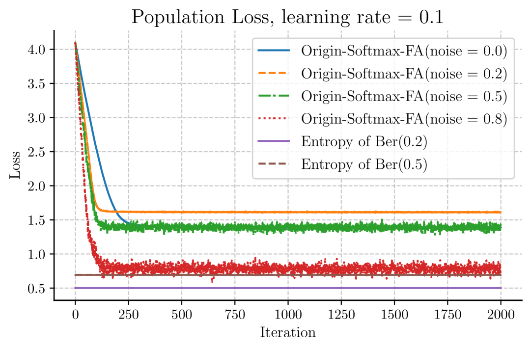
(a)

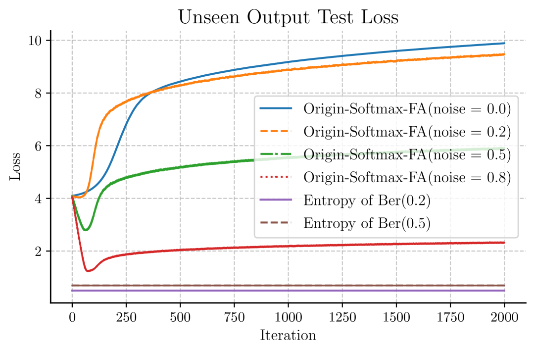
(b)

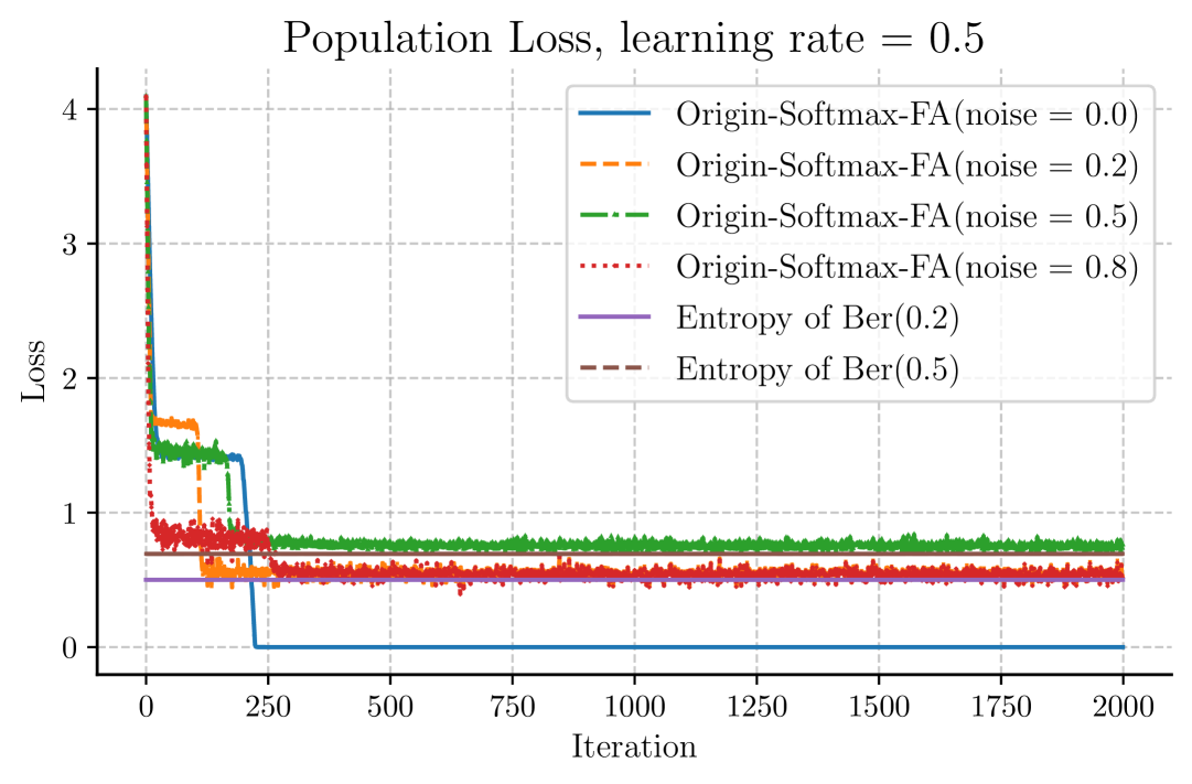
(c)

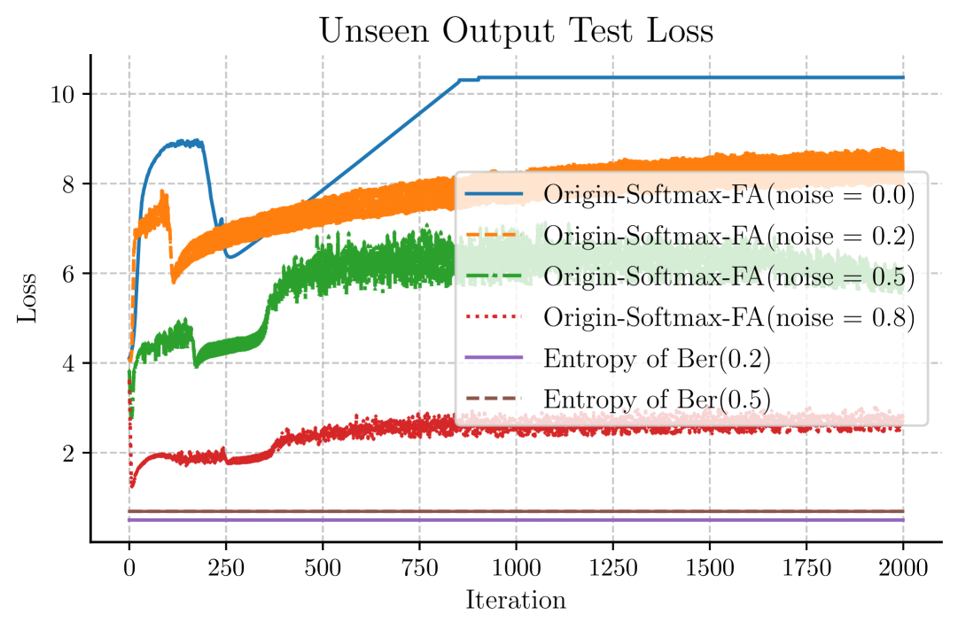
(d)

Figure 3: Population and Unseen Output Test Losses of Origin-Softmax-FA with $\eta=0.1$ (first row), $\eta=0.1$ (second row). The population losses do not converge at $\eta=0.1$ but converges at $\eta=0.5$. Generalization to unseen output words is non-existent.

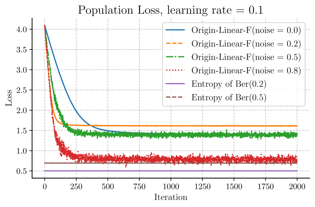
(a)

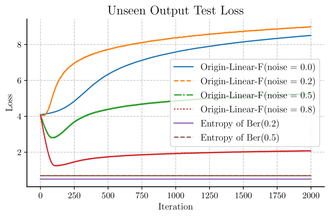
(b)

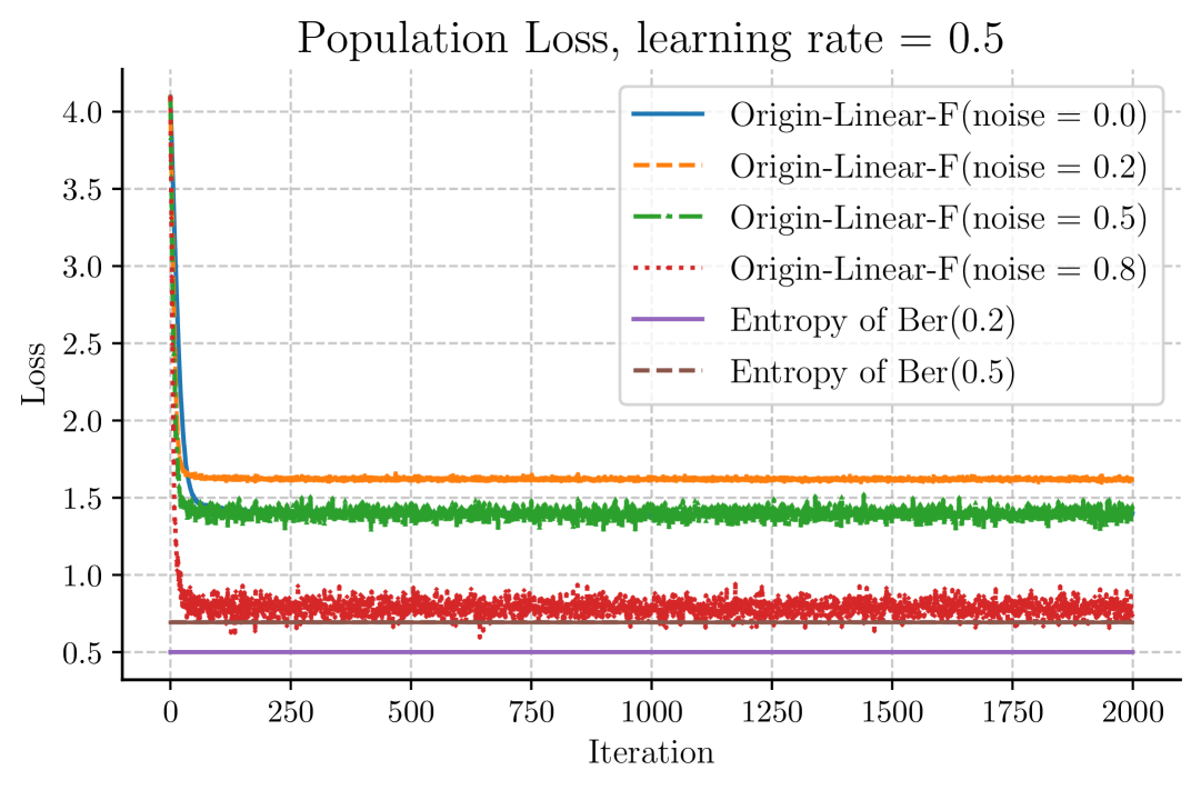
(c)

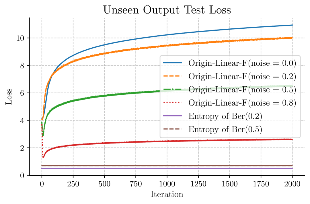
(d)

Figure 4: Population and Unseen Output Test Losses of Origin-Linear-F with $\eta=0.1$ (first row), $\eta=0.1$ (second row). The population losses do not converge at neither $\eta=0.1$ nor $\eta=0.5$. Generalization to unseen output words is non-existent.

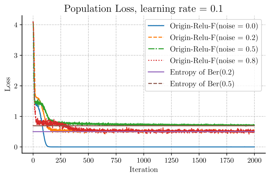
(a)

(b)

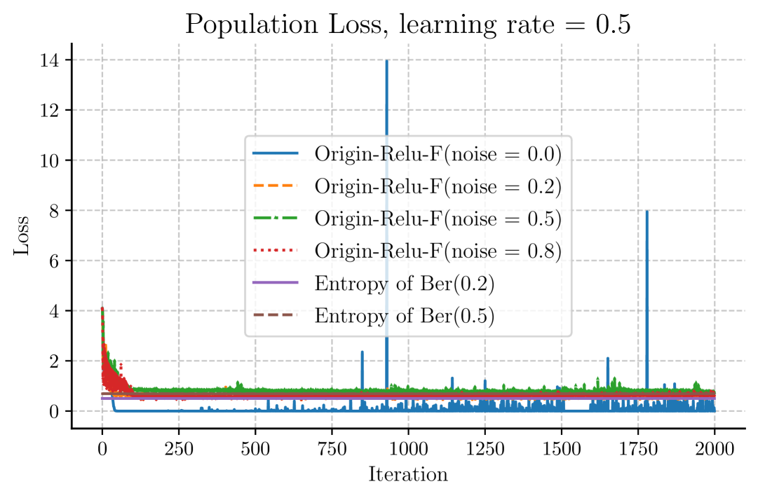
(c)

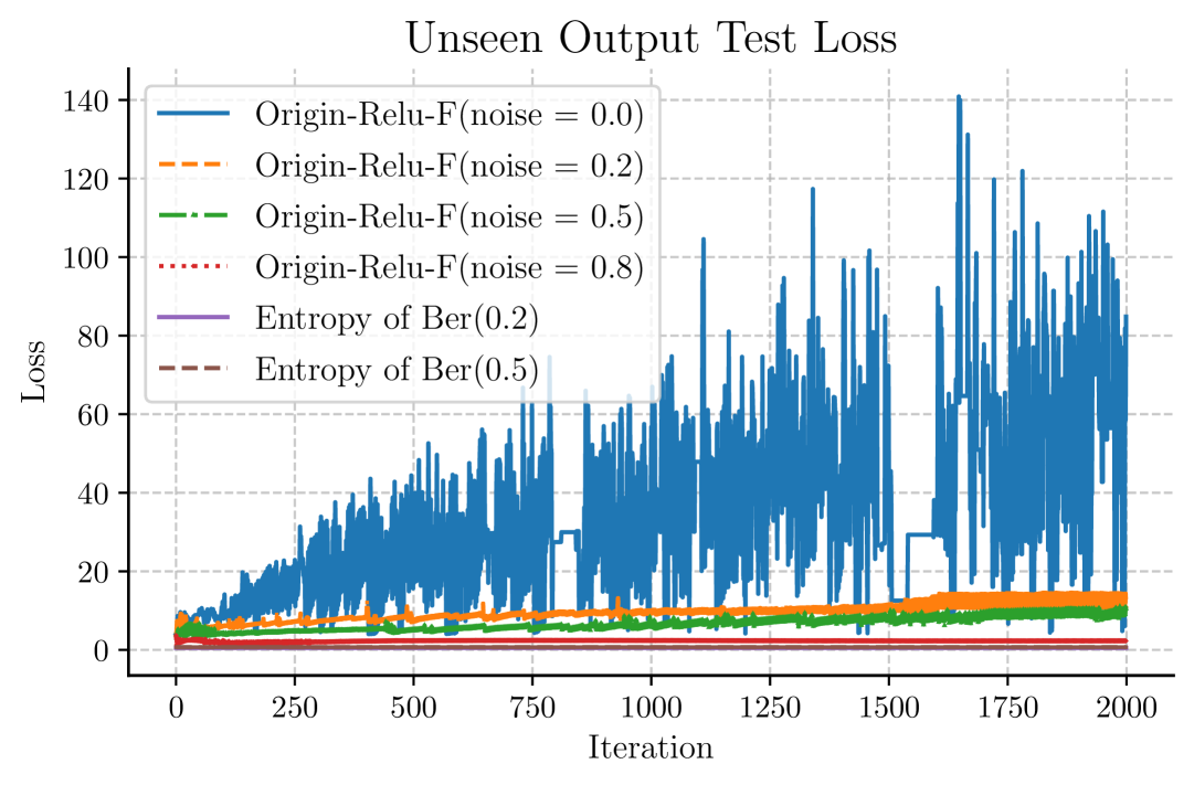
(d)

Figure 5: Population and Unseen Output Test Losses of Origin-ReLU-F with $\eta=0.1$ (first row), $\eta=0.5$ (second row). The population losses converge at $\eta=0.1$ but do not converge at $\eta=0.5$. Generalization to unseen output words is non-existent.

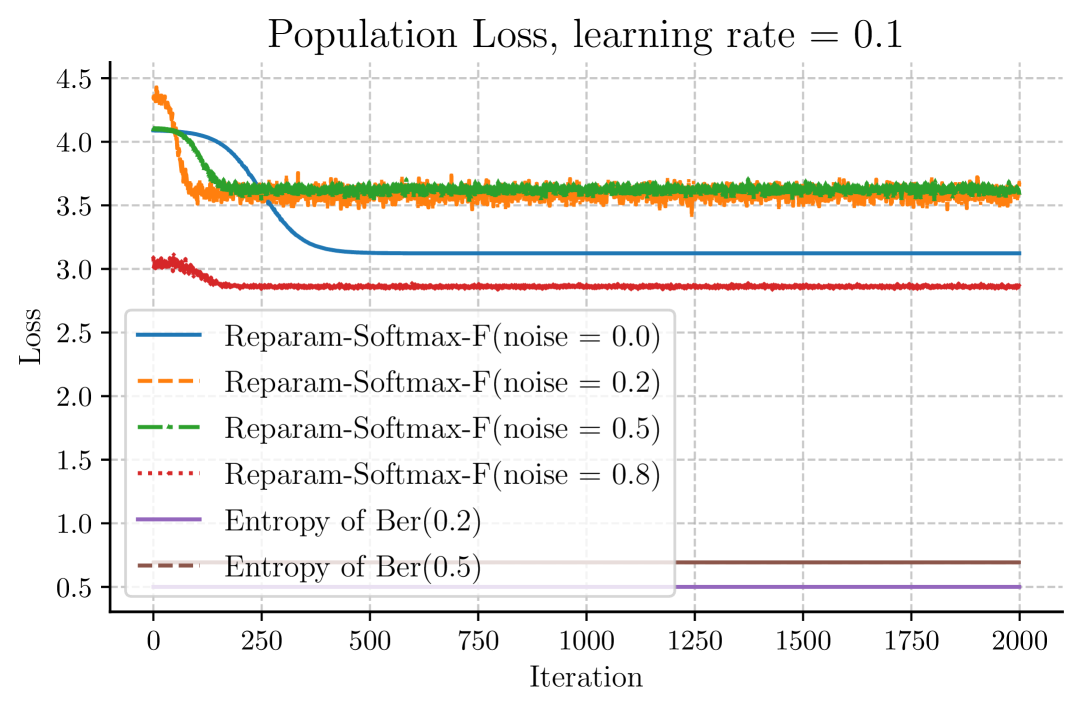
(a)

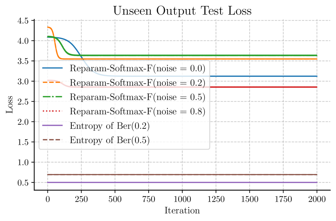
(b)

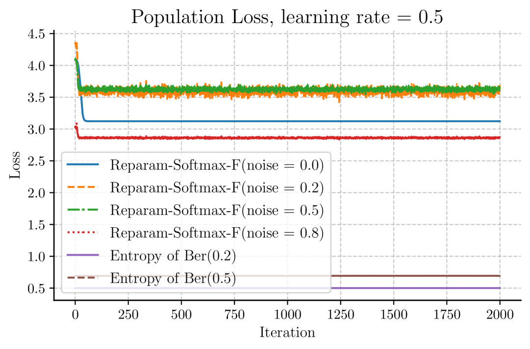
(c)

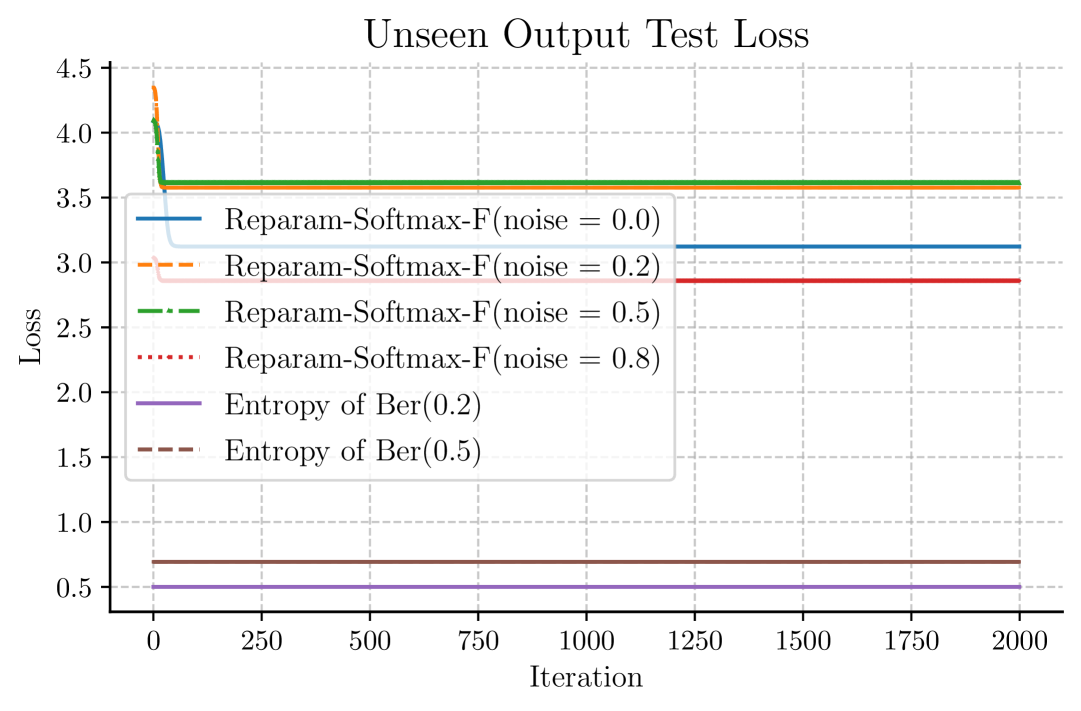
(d)

Figure 6: Population and Unseen Output Test Losses of Reparam-Softmax-F with $\eta=0.1$ (first row), $\eta=0.5$ (second row). The population losses do not converge at neither $\eta=0.1$ nor $\eta=0.5$. The model has a high degree of generalization to unseen output words.

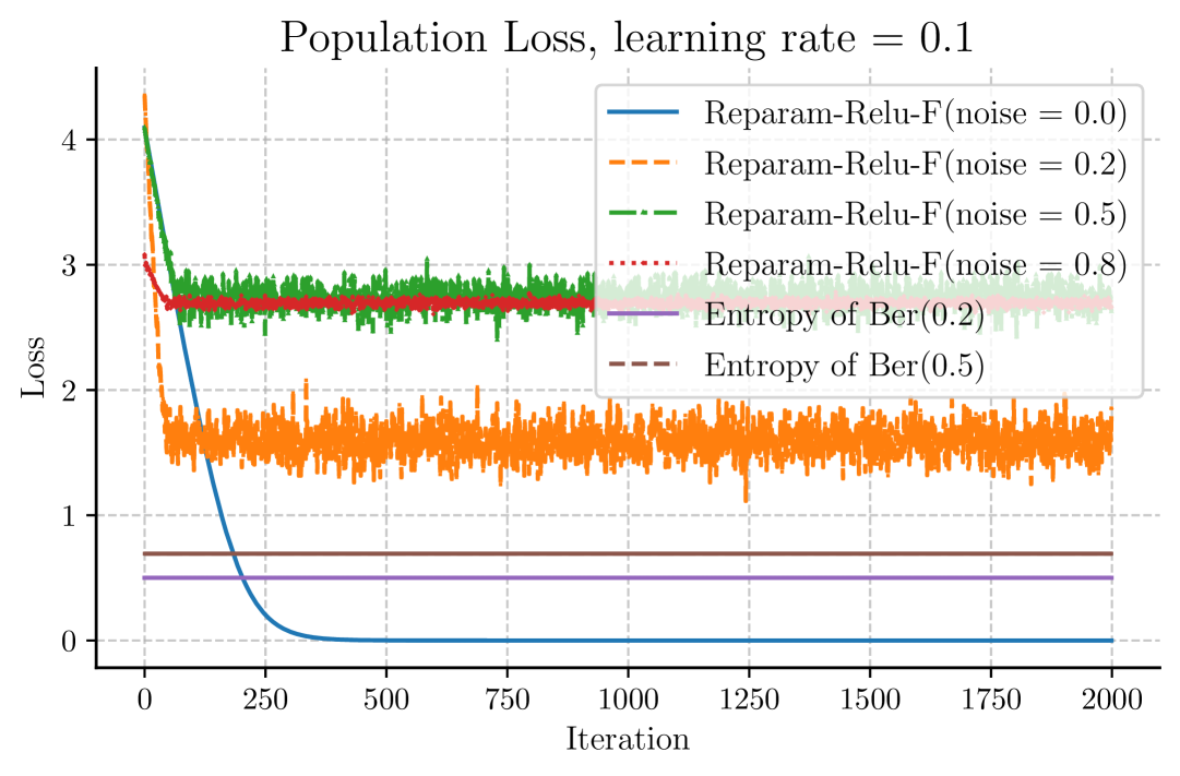
(a)

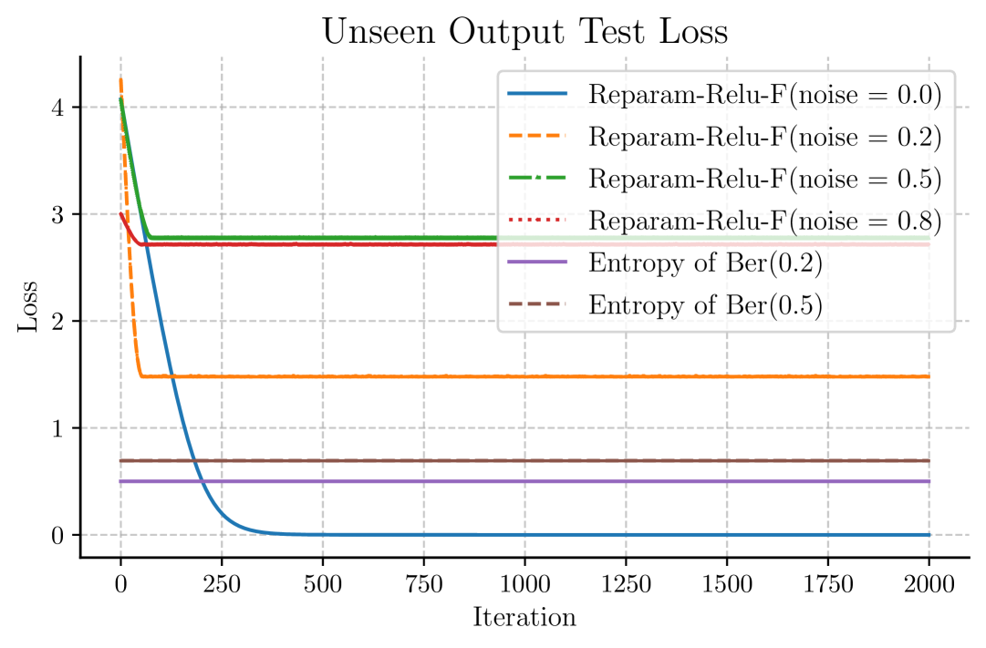
(b)

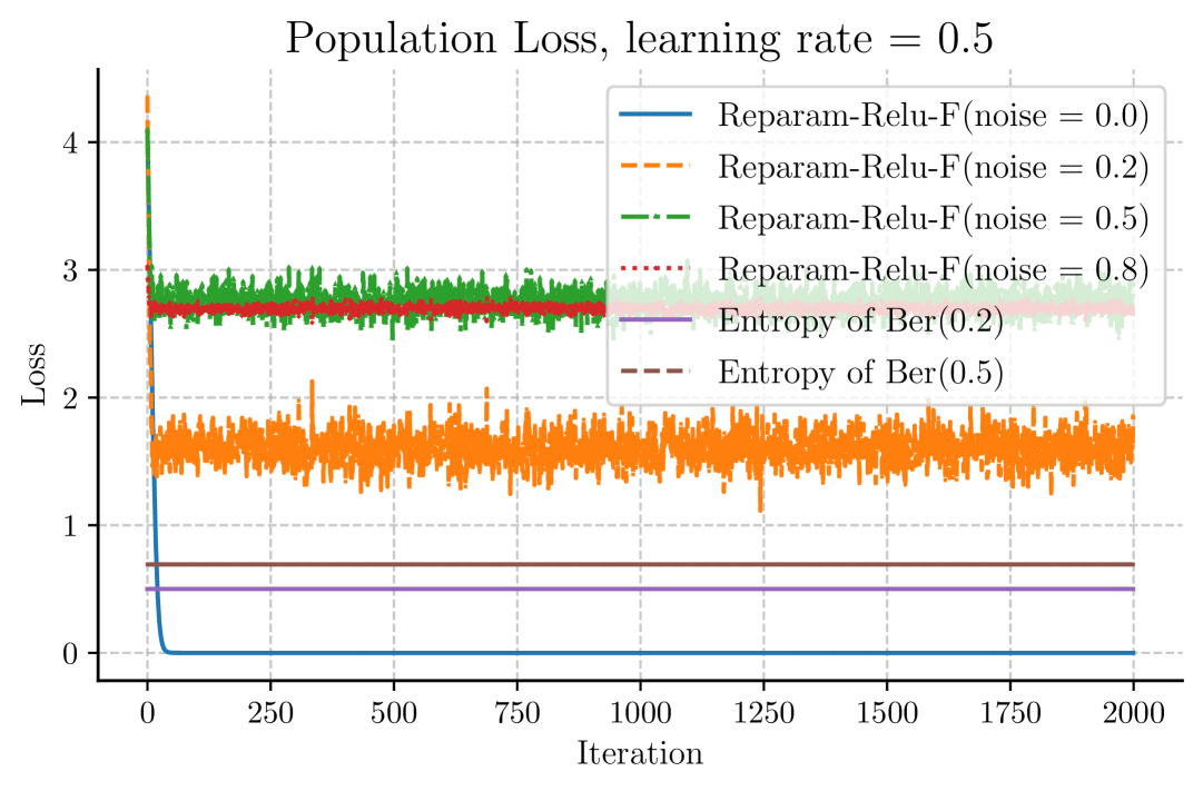
(c)

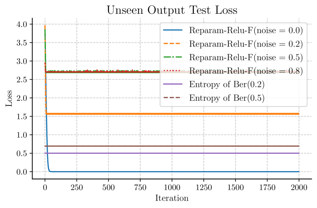
(d)

Figure 7: Population and Unseen Output Test Losses of Reparam-ReLU-F with $\eta=0.1$ (first row), $\eta=0.5$ (second row). The population loss for noiseless setting converges at both $\eta=0.1$ nor $\eta=0.5$. All noisy population losses never converge for any learning rate. The model has a high degree of generalization to unseen output words.

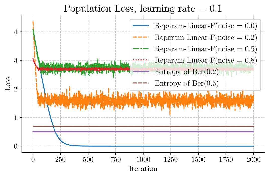
(a)

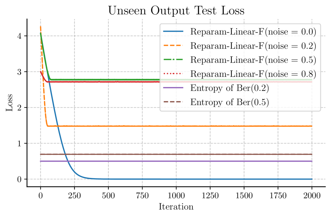
(b)

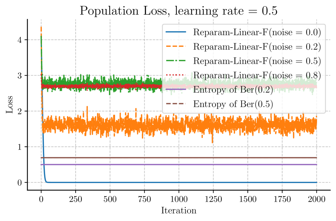
(c)

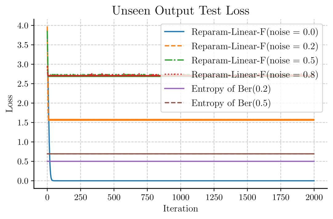
(d)

Figure 8: Population and Unseen Output Test Losses of Reparam-Linear-F with $\eta=0.1$ (first row), $\eta=0.5$ (second row). The population loss for noiseless setting converges at both $\eta=0.1$ nor $\eta=0.5$. All noisy population losses never converge for any learning rate. The model has a high degree of generalization to unseen output words.

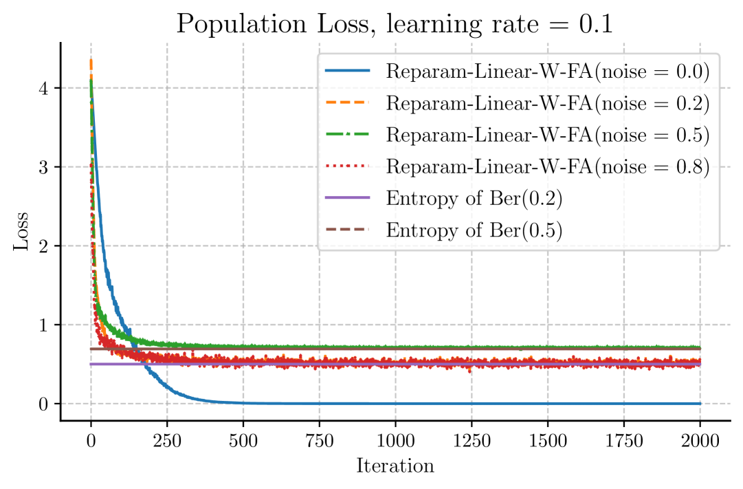
(a)

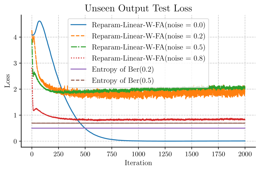
(b)

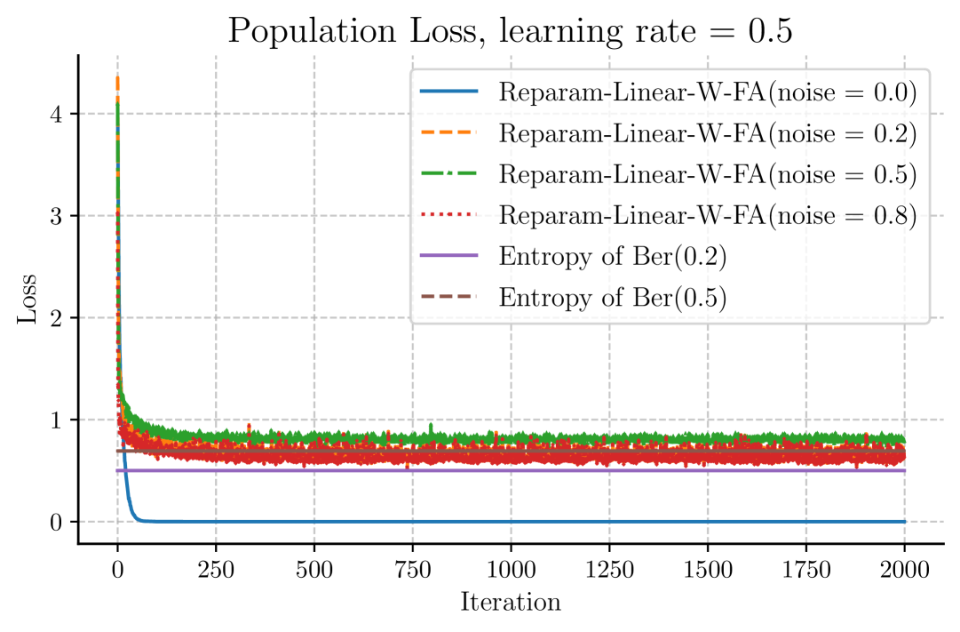
(c)

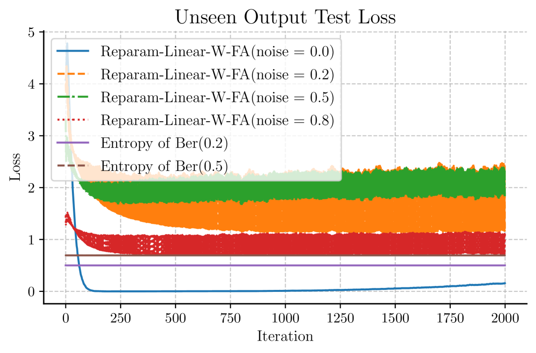
(d)

Figure 9: Population and Unseen Output Test Losses of Reparam-Linear-W-FA with $\eta=0.1$ (first row), $\eta=0.5$ (second row). Population losses converge with limited generalization to unseen output words.

D.2.2 Attention Layer Learns to Predict Output Tokens while Feed-Forward Layer Learns to Predict Noise Token

To measure the extent to which we can separate the learning functionality of the attention layer and the feed-forward layer, we train three models Origin-Linear-FA, Reparam-Linear-FA and Reparam-Linear-W-FA, and record the logits of each layer on the output tokens, the noise tokens and the maximum values in the logits of the two layers on all three noisy tasks with $\alpha=0.2,0.5$ and $0.8$. We use $\eta=0.1$ in all experiments. The results are reported in Figures 10 to 12.

We say that the attention layer and the feed-forward layer learns to predict the output and noise tokens, respectively, if $\xi_{A,y}=\max_{j}\xi_{A,j}$ and $\xi_{F,\tau}=\max_{j}\xi_{F,\tau}$. It can be observed that all three models exhibit some layer-specific learning mechanism, including the original model where all three matrices ${\bm{V}},{\bm{W}}$ and ${\bm{F}}$ are trained from scratch without reparameterization. However, depending on the noise level, at least one of the two layers in the original model do not fully specialize in either the output nor the noise tokens. For $\alpha\leq 0.5$, Figures 10(a) and 10(d) show that the attention layer in Origin-Softmax-FA learns to predict output tokens perfectly, however the feed-forward layer does not always predict $\tau$. At $\alpha=0.8$, the feed-forward layer succeeds in learning to predict $\tau$ but the attention layer fails to focus entirely on the output tokens.

In contrast, the fully-reparameterized model Reparam-Linear-FA exhibits perfect separation in the functionality of the two layers, which verified our Theorem 4.5. The same phenomenon is also observed in Reparam-Linear-W-FA, which suggests that reparameterizing ${\bm{F}}$ is sufficient to force the two layers to be biased towards two different types of tokens.

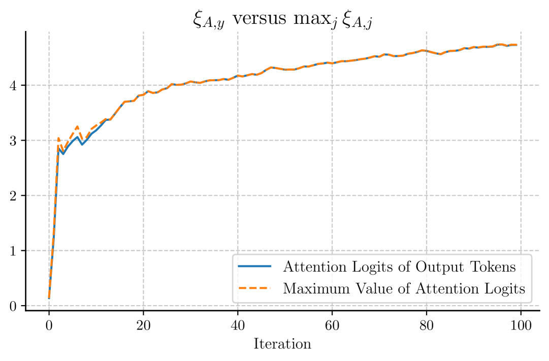
(a)

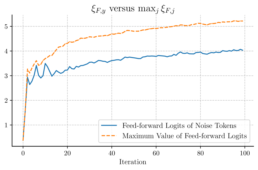
(b)

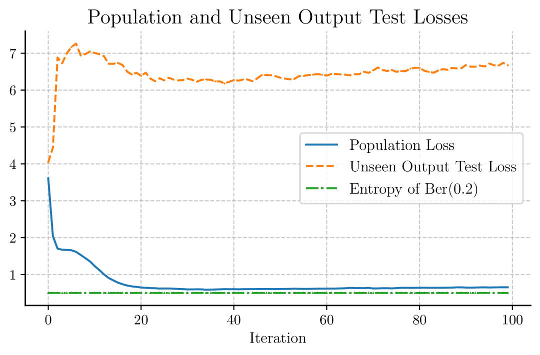
(c)

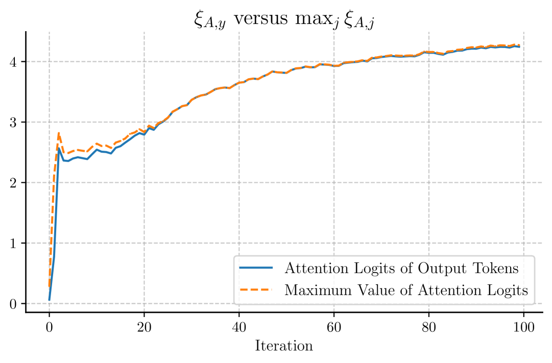
(d)

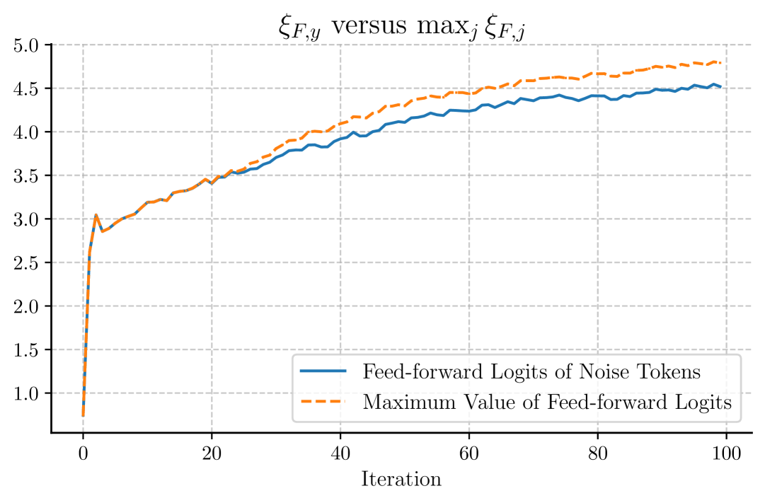
(e)

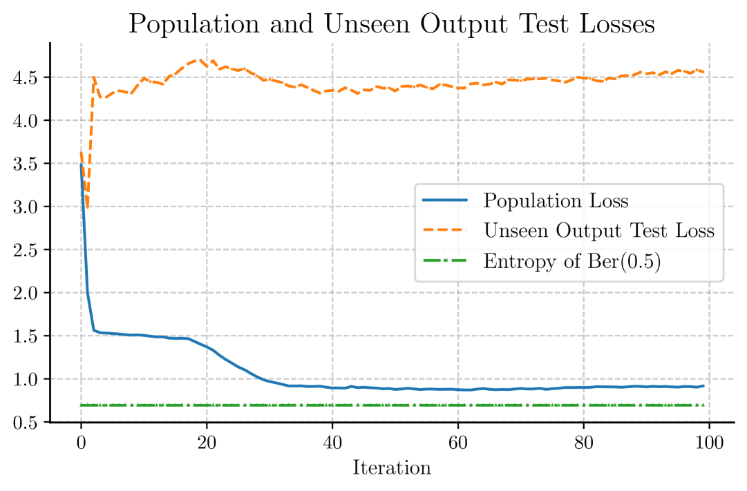
(f)

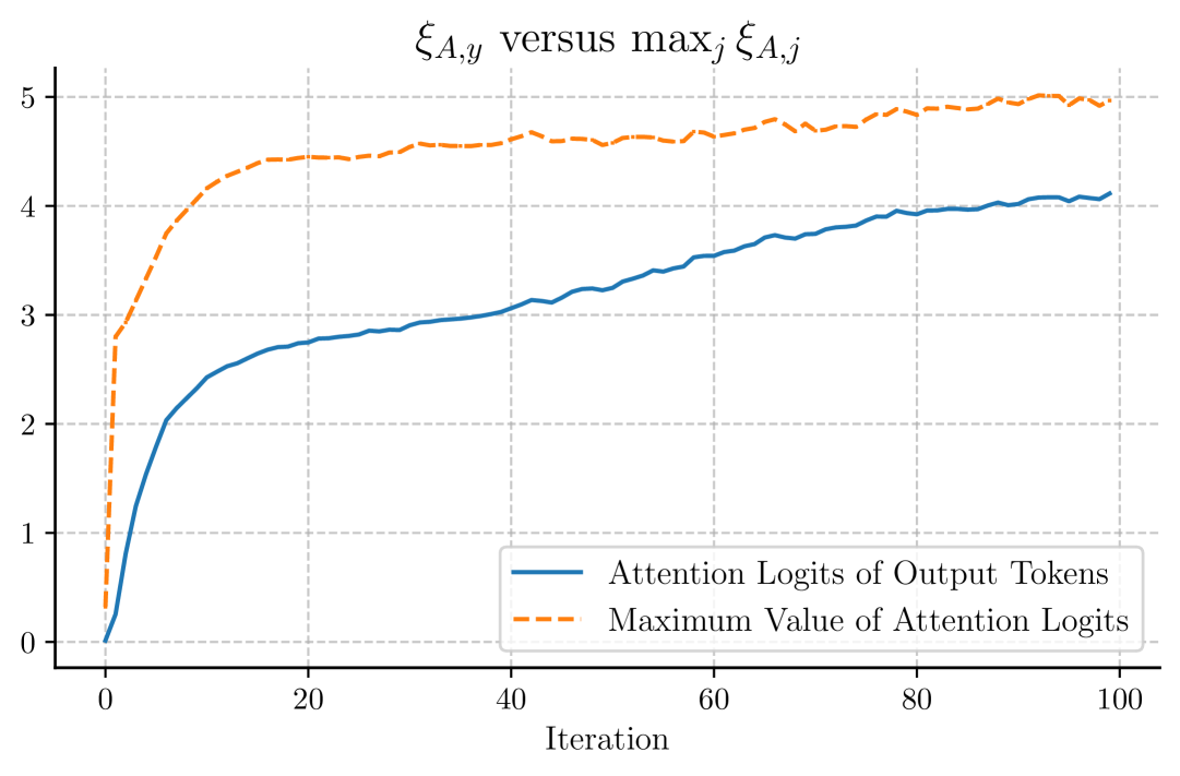
(g)

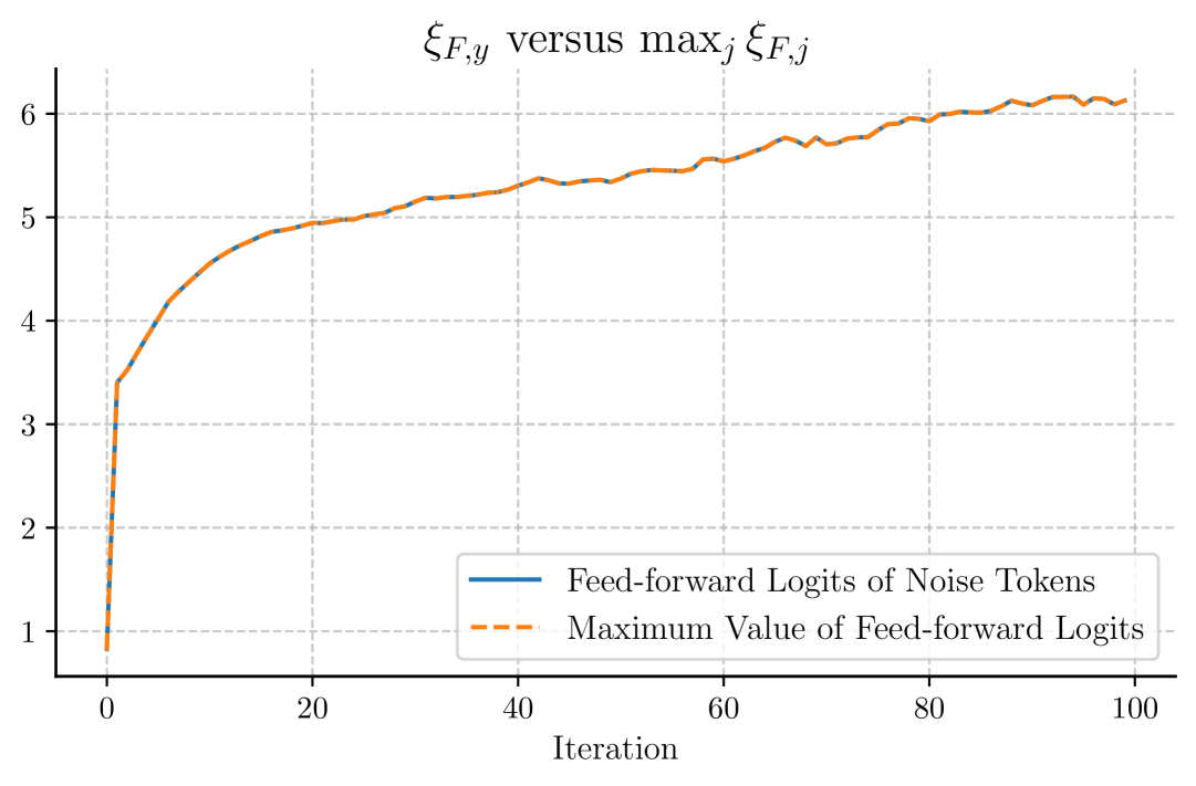
(h)

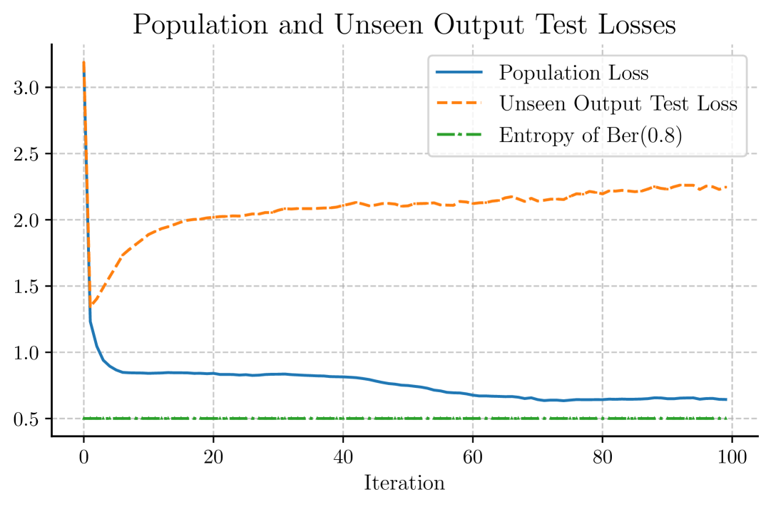
(i)

Figure 10: Origin-Linear-FA with $\alpha=0.2$ (first row), $\alpha=0.5$ (second row) and $\alpha=0.8$ (third row). The learning rate is $\eta=0.1$.

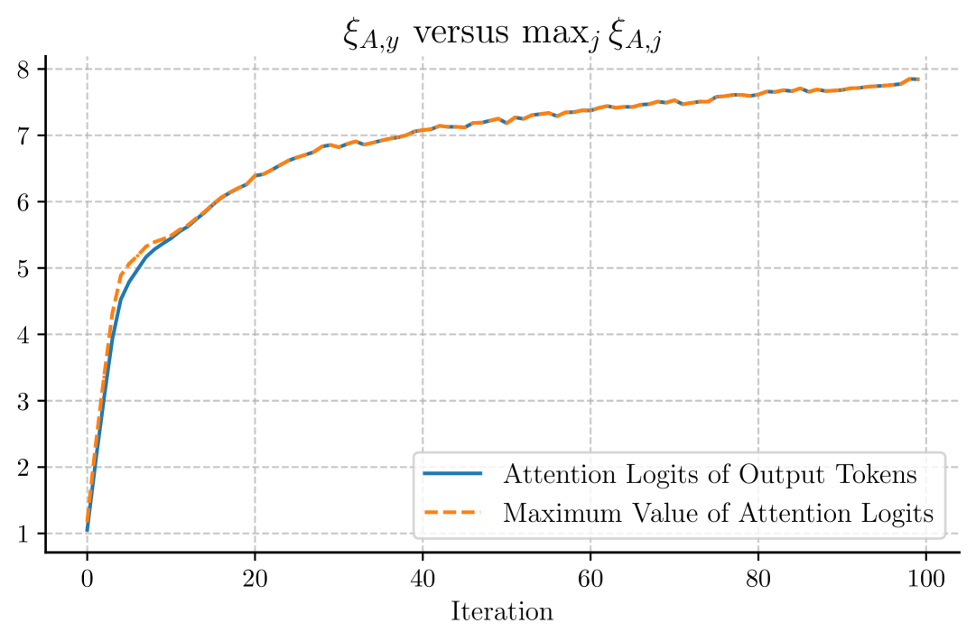
(a)

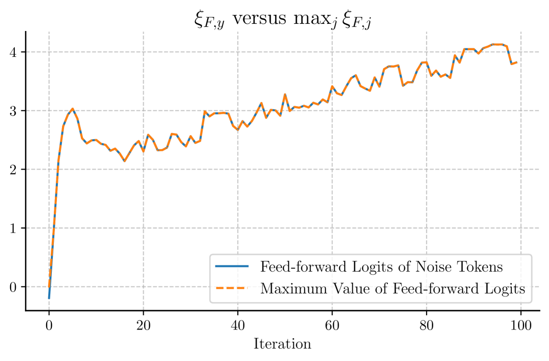
(b)

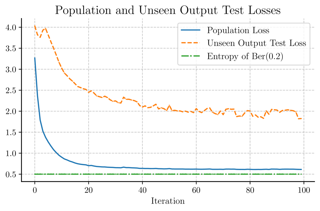
(c)

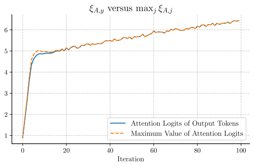
(d)

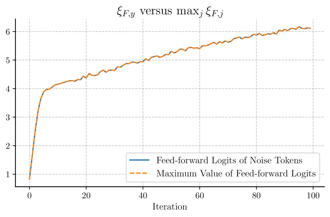
(e)

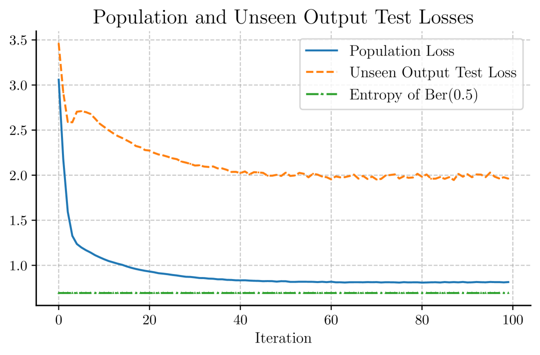
(f)

(g)

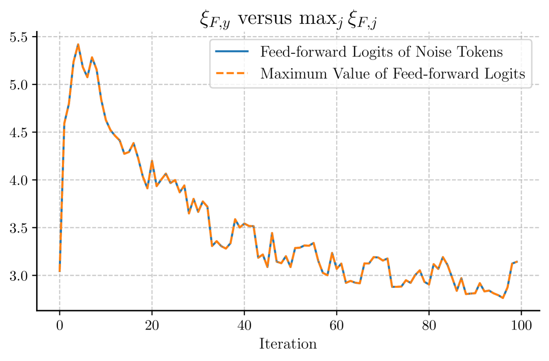
(h)

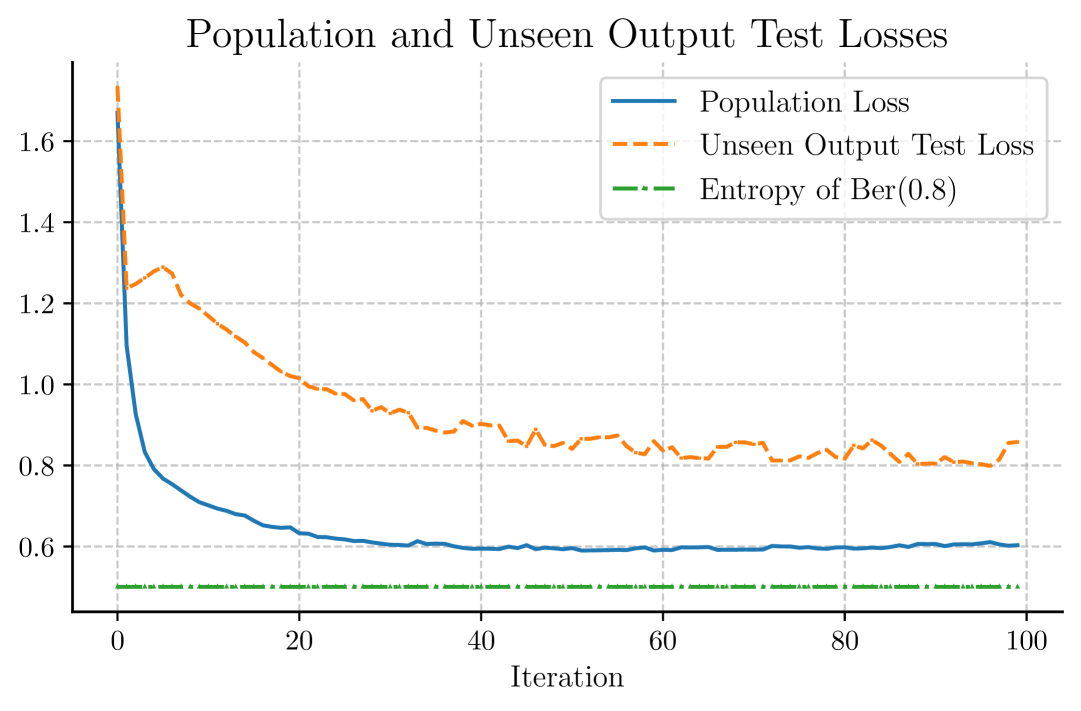
(i)

Figure 11: Reparam-Linear-W-FA with $\alpha=0.2$ (first row), $\alpha=0.5$ (second row) and $\alpha=0.8$ (third row). The learning rate is $\eta=0.1$.

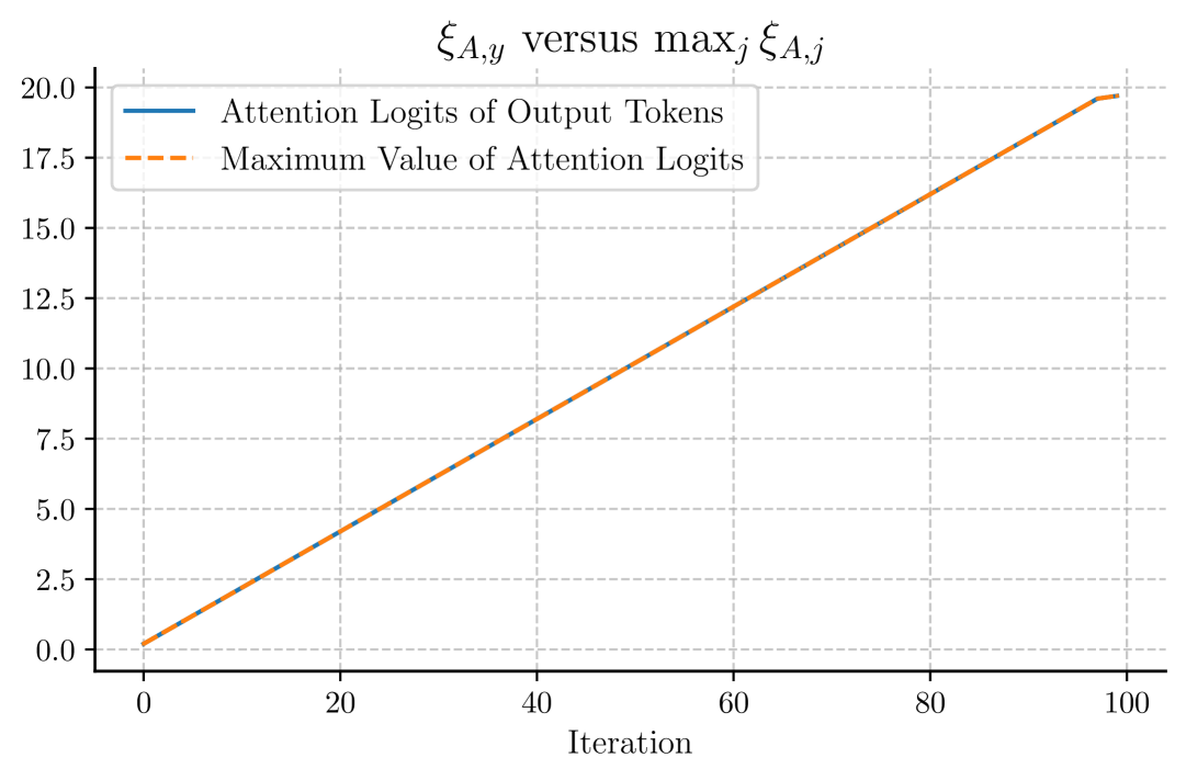
(a)

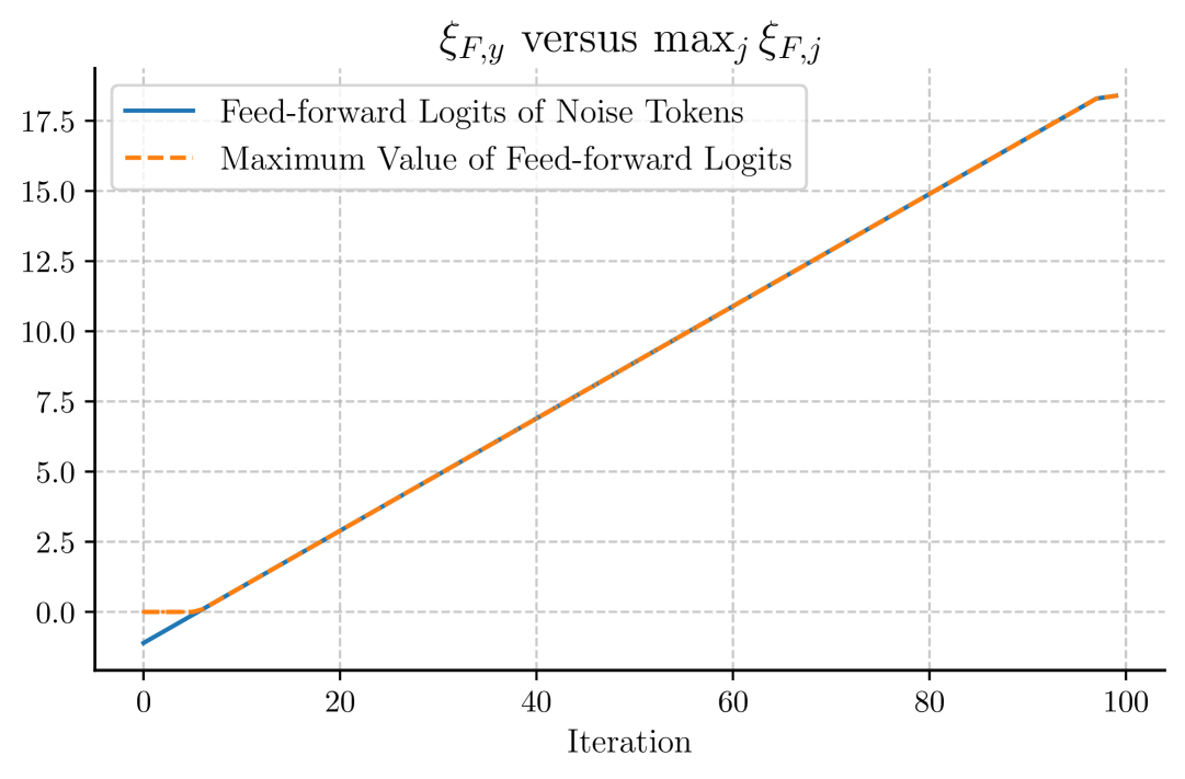
(b)

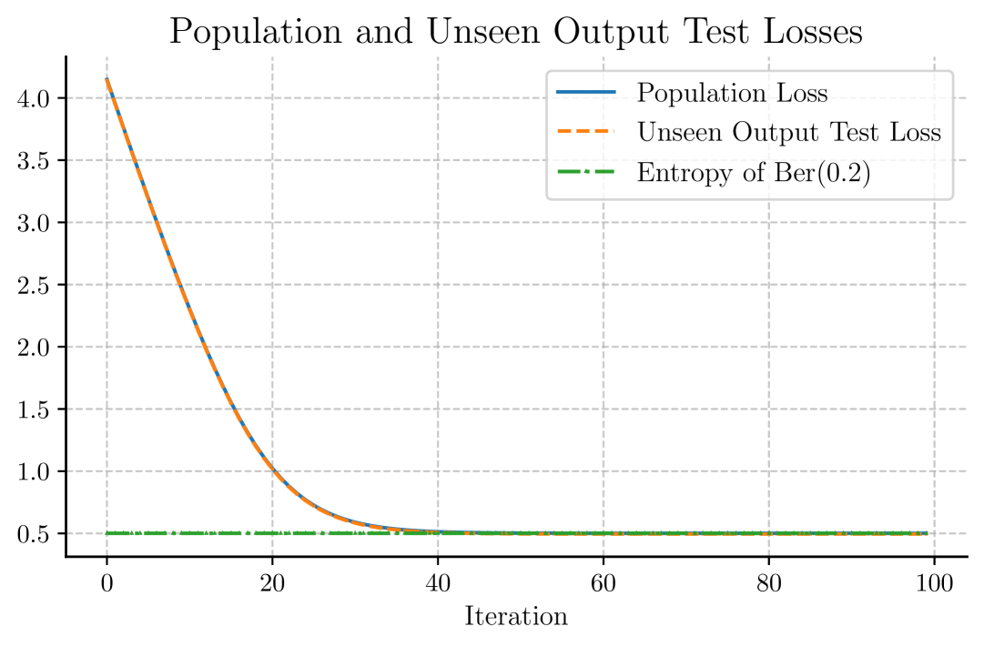
(c)

(d)

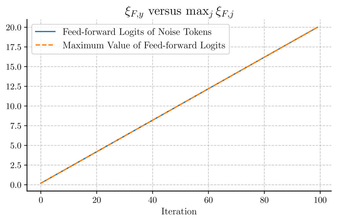
(e)

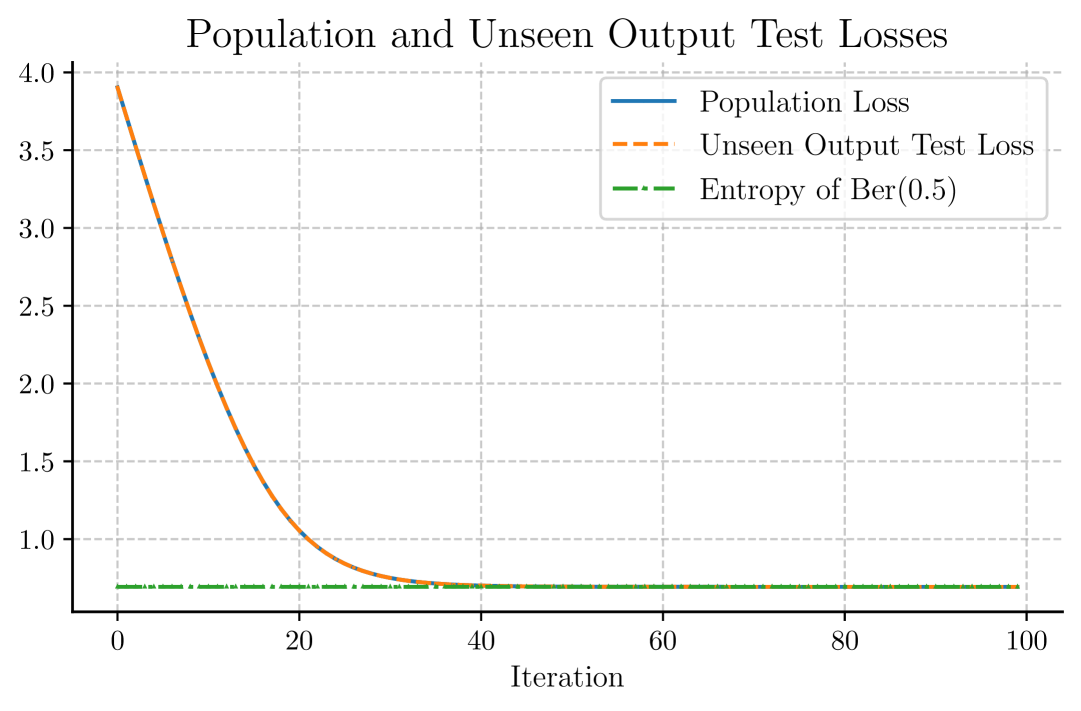
(f)

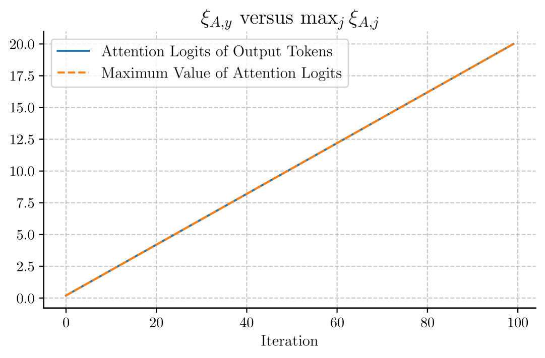
(g)

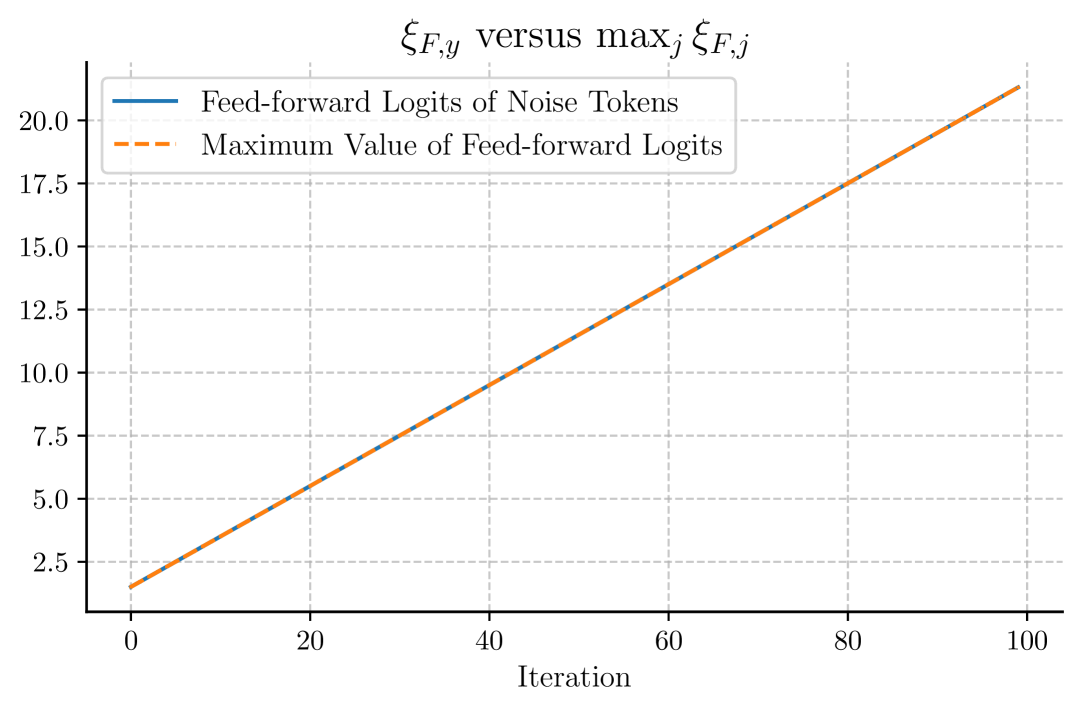
(h)

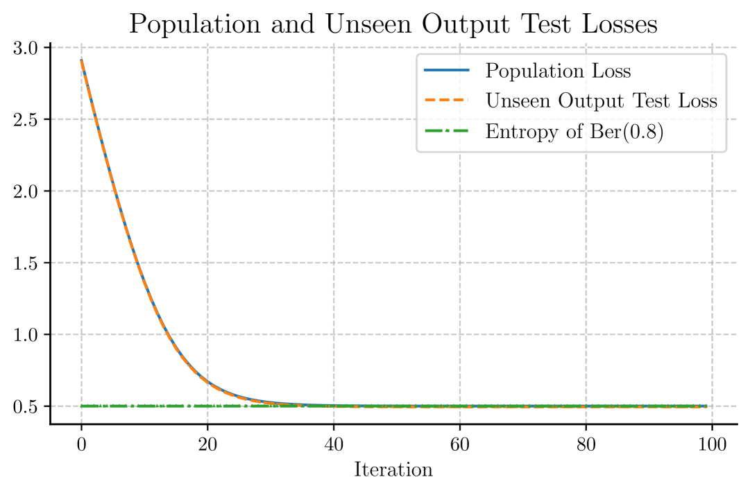
(i)

Figure 12: Reparam-Linear-FA with $\alpha=0.2$ (first row), $\alpha=0.5$ (second row) and $\alpha=0.8$ (third row). The learning rate is $\eta=0.1$.

References

- Brown et al. [2020] Tom Brown, Benjamin Mann, Nick Ryder, Melanie Subbiah, Jared D Kaplan, Prafulla Dhariwal, Arvind Neelakantan, Pranav Shyam, Girish Sastry, Amanda Askell, et al. Language models are few-shot learners. Advances in neural information processing systems, 33:1877–1901, 2020.
- Achiam et al. [2023] Josh Achiam, Steven Adler, Sandhini Agarwal, Lama Ahmad, Ilge Akkaya, Florencia Leoni Aleman, Diogo Almeida, Janko Altenschmidt, Sam Altman, Shyamal Anadkat, et al. Gpt-4 technical report. arXiv preprint arXiv:2303.08774, 2023.
- Vaswani et al. [2017] Ashish Vaswani, Noam Shazeer, Niki Parmar, Jakob Uszkoreit, Llion Jones, Aidan N Gomez, Łukasz Kaiser, and Illia Polosukhin. Attention is all you need. Advances in neural information processing systems, 30, 2017.
- Bommasani et al. [2021] Rishi Bommasani, Drew A Hudson, Ehsan Adeli, Russ Altman, Simran Arora, Sydney von Arx, Michael S Bernstein, Jeannette Bohg, Antoine Bosselut, Emma Brunskill, et al. On the opportunities and risks of foundation models. arXiv preprint arXiv:2108.07258, 2021.
- Belkin [2024] Mikhail Belkin. The necessity of machine learning theory in mitigating ai risk. ACM/IMS Journal of Data Science, 1(3):1–6, 2024.
- Allen-Zhu [2024] Zeyuan Allen-Zhu. ICML 2024 Tutorial: Physics of Language Models, July 2024. Project page: https://physics.allen-zhu.com/.
- Chen et al. [2025] Lei Chen, Joan Bruna, and Alberto Bietti. Distributional associations vs in-context reasoning: A study of feed-forward and attention layers. In The Thirteenth International Conference on Learning Representations, 2025. URL https://openreview.net/forum?id=WCVMqRHWW5.
- Wang et al. [2022] Kevin Wang, Alexandre Variengien, Arthur Conmy, Buck Shlegeris, and Jacob Steinhardt. Interpretability in the wild: a circuit for indirect object identification in gpt-2 small. arXiv preprint arXiv:2211.00593, 2022.
- Geva et al. [2020] Mor Geva, Roei Schuster, Jonathan Berant, and Omer Levy. Transformer feed-forward layers are key-value memories. arXiv preprint arXiv:2012.14913, 2020.
- Meng et al. [2022] Kevin Meng, David Bau, Alex Andonian, and Yonatan Belinkov. Locating and editing factual associations in gpt. Advances in neural information processing systems, 35:17359–17372, 2022.
- Bietti et al. [2023] Alberto Bietti, Vivien Cabannes, Diane Bouchacourt, Herve Jegou, and Leon Bottou. Birth of a transformer: A memory viewpoint. In Thirty-seventh Conference on Neural Information Processing Systems, 2023. URL https://openreview.net/forum?id=3X2EbBLNsk.
- Nichani et al. [2024] Eshaan Nichani, Jason D Lee, and Alberto Bietti. Understanding factual recall in transformers via associative memories. arXiv preprint arXiv:2412.06538, 2024.
- Akyürek et al. [2022] Ekin Akyürek, Dale Schuurmans, Jacob Andreas, Tengyu Ma, and Denny Zhou. What learning algorithm is in-context learning? investigations with linear models. arXiv preprint arXiv:2211.15661, 2022.
- Bai et al. [2023] Yu Bai, Fan Chen, Huan Wang, Caiming Xiong, and Song Mei. Transformers as statisticians: Provable in-context learning with in-context algorithm selection. Advances in neural information processing systems, 36:57125–57211, 2023.
- Von Oswald et al. [2023] Johannes Von Oswald, Eyvind Niklasson, Ettore Randazzo, João Sacramento, Alexander Mordvintsev, Andrey Zhmoginov, and Max Vladymyrov. Transformers learn in-context by gradient descent. In International Conference on Machine Learning, pages 35151–35174. PMLR, 2023.
- Giannou et al. [2023] Angeliki Giannou, Shashank Rajput, Jy-yong Sohn, Kangwook Lee, Jason D Lee, and Dimitris Papailiopoulos. Looped transformers as programmable computers. In International Conference on Machine Learning, pages 11398–11442. PMLR, 2023.
- Yun et al. [2019] Chulhee Yun, Srinadh Bhojanapalli, Ankit Singh Rawat, Sashank J Reddi, and Sanjiv Kumar. Are transformers universal approximators of sequence-to-sequence functions? arXiv preprint arXiv:1912.10077, 2019.
- Ahn et al. [2024] Kwangjun Ahn, Xiang Cheng, Minhak Song, Chulhee Yun, Ali Jadbabaie, and Suvrit Sra. Linear attention is (maybe) all you need (to understand transformer optimization). In The Twelfth International Conference on Learning Representations, 2024. URL https://openreview.net/forum?id=0uI5415ry7.
- Mahankali et al. [2023] Arvind Mahankali, Tatsunori B Hashimoto, and Tengyu Ma. One step of gradient descent is provably the optimal in-context learner with one layer of linear self-attention. arXiv preprint arXiv:2307.03576, 2023.
- Zhang et al. [2024] Ruiqi Zhang, Spencer Frei, and Peter L Bartlett. Trained transformers learn linear models in-context. Journal of Machine Learning Research, 25(49):1–55, 2024.
- Huang et al. [2024a] Yu Huang, Yuan Cheng, and Yingbin Liang. In-context convergence of transformers. In Proceedings of the 41st International Conference on Machine Learning, ICML’24. JMLR.org, 2024a.
- Cui et al. [2024] Yingqian Cui, Jie Ren, Pengfei He, Jiliang Tang, and Yue Xing. Superiority of multi-head attention in in-context linear regression. arXiv preprint arXiv:2401.17426, 2024.
- Cheng et al. [2023] Xiang Cheng, Yuxin Chen, and Suvrit Sra. Transformers implement functional gradient descent to learn non-linear functions in context. arXiv preprint arXiv:2312.06528, 2023.
- Kim and Suzuki [2024] Juno Kim and Taiji Suzuki. Transformers learn nonlinear features in context: Nonconvex mean-field dynamics on the attention landscape. arXiv preprint arXiv:2402.01258, 2024.
- Chen and Li [2024] Sitan Chen and Yuanzhi Li. Provably learning a multi-head attention layer. arXiv preprint arXiv:2402.04084, 2024.
- Tarzanagh et al. [2023] Davoud Ataee Tarzanagh, Yingcong Li, Christos Thrampoulidis, and Samet Oymak. Transformers as support vector machines. arXiv preprint arXiv:2308.16898, 2023.
- Ataee Tarzanagh et al. [2023] Davoud Ataee Tarzanagh, Yingcong Li, Xuechen Zhang, and Samet Oymak. Max-margin token selection in attention mechanism. Advances in neural information processing systems, 36:48314–48362, 2023.
- Vasudeva et al. [2024] Bhavya Vasudeva, Puneesh Deora, and Christos Thrampoulidis. Implicit bias and fast convergence rates for self-attention. arXiv preprint arXiv:2402.05738, 2024.
- Deora et al. [2023] Puneesh Deora, Rouzbeh Ghaderi, Hossein Taheri, and Christos Thrampoulidis. On the optimization and generalization of multi-head attention. arXiv preprint arXiv:2310.12680, 2023.
- Tian et al. [2023a] Yuandong Tian, Yiping Wang, Beidi Chen, and Simon S Du. Scan and snap: Understanding training dynamics and token composition in 1-layer transformer. Advances in neural information processing systems, 36:71911–71947, 2023a.
- Tian et al. [2023b] Yuandong Tian, Yiping Wang, Zhenyu Zhang, Beidi Chen, and Simon Du. Joma: Demystifying multilayer transformers via joint dynamics of mlp and attention. arXiv preprint arXiv:2310.00535, 2023b.
- Li et al. [2024] Yingcong Li, Yixiao Huang, Muhammed E Ildiz, Ankit Singh Rawat, and Samet Oymak. Mechanics of next token prediction with self-attention. In International Conference on Artificial Intelligence and Statistics, pages 685–693. PMLR, 2024.
- Thrampoulidis [2024] Christos Thrampoulidis. Implicit optimization bias of next-token prediction in linear models. arXiv preprint arXiv:2402.18551, 2024.
- Huang et al. [2024b] Ruiquan Huang, Yingbin Liang, and Jing Yang. Non-asymptotic convergence of training transformers for next-token prediction. In The Thirty-eighth Annual Conference on Neural Information Processing Systems, 2024b. URL https://openreview.net/forum?id=NfOFbPpYII.
- Mahdavi et al. [2023] Sadegh Mahdavi, Renjie Liao, and Christos Thrampoulidis. Memorization capacity of multi-head attention in transformers. arXiv preprint arXiv:2306.02010, 2023.
- Madden et al. [2024] Liam Madden, Curtis Fox, and Christos Thrampoulidis. Next-token prediction capacity: general upper bounds and a lower bound for transformers. arXiv preprint arXiv:2405.13718, 2024.
- von Oswald et al. [2024] Johannes von Oswald, Maximilian Schlegel, Alexander Meulemans, Seijin Kobayashi, Eyvind Niklasson, Nicolas Zucchet, Nino Scherrer, Nolan Miller, Mark Sandler, Blaise Agüera y Arcas, Max Vladymyrov, Razvan Pascanu, and João Sacramento. Uncovering mesa-optimization algorithms in transformers, 2024. URL https://arxiv.org/abs/2309.05858.
- Ji and Telgarsky [2021] Ziwei Ji and Matus Telgarsky. Characterizing the implicit bias via a primal-dual analysis. In Vitaly Feldman, Katrina Ligett, and Sivan Sabato, editors, Proceedings of the 32nd International Conference on Algorithmic Learning Theory, volume 132 of Proceedings of Machine Learning Research, pages 772–804. PMLR, 16–19 Mar 2021. URL https://proceedings.mlr.press/v132/ji21a.html.
- Nemirovski et al. [2009] A. Nemirovski, A. Juditsky, G. Lan, and A. Shapiro. Robust stochastic approximation approach to stochastic programming. SIAM Journal on Optimization, 19(4):1574–1609, 2009. doi: 10.1137/070704277. URL https://doi.org/10.1137/070704277.
- Dud´ık et al. [2022] Miroslav Dudík, Ziwei Ji, Robert Schapire, and Matus Telgarsky. Convex analysis at infinity: An introduction to astral space. 05 2022. doi: 10.48550/arXiv.2205.03260.
- Sason [2015] Igal Sason. On reverse Pinsker inequalities. arXiv preprint arXiv:1503.07118, 2015.